Neural Process Lett (2017) 46:1059–1081DOI 10.1007/s11063-017-9627-1

A Hybrid Model Equipped with the Minimum CycleDecomposition Concept for Short-Term Forecastingof Electrical Load Time Series

Zhaoshuang He1 · Caihong Li1 · Yulin Shen2 ·Anping He1

Published online: 10 April 2017© The Author(s) 2017. This article is an open access publication

Abstract Electricity load forecasting is an essential, however complicated work. Due to theinfluence of a large number of uncertain factors, it shows complicated nonlinear combinationfeatures. Therefore, it is difficult to improve the prediction accuracy and the tremendousbreadth of applicability especially for using a single method. In order to improve the perfor-mance including accuracy and applicability of electricity load forecasting, in this paper, aconcept named minimum cycle decomposition (MCD) that the raw data are grouped accord-ing to the minimum cycle was proposed for the first time. In addition, a hybrid predictionmodel (HMM) based on one-order difference, ensemble empirical model decomposition(EEMD), mind evolutionary computation (MEC) and wavelet neural network (WNN) wasalso proposed in this study. The HMMmodel consists of two parts. Part one, pre-processing,known as one order difference to remove the trend of subsequence and EEMD to reducethe noise, was performed by HMM model on each subset. Part two, the WNN optimizedby MEC (WNN + MEC) was applied on resultant subseries. Finally, a number of differentmodels were used as the comparative experiment to validate the effectiveness of the presentedmethod, such as back propagation neural network (BP-1), BPNN combined MCD (BP-2),WNN combined MCD (WNNM), a HMM (DEEPLSSVM) based on one-order difference,EEMD, particle swarm optimization and least squares support vector machine and a hybridmodel (DEESGRNN) based on one-order difference, EEMD, simulate anneal and gener-alized regression neural network. Certain evaluation measurements are taken into accountto assess the performance. Experiments were carried out on QLD (Queensland) and NSW(New South Wales) electricity markets historical data, and the experimental results showthat the MCD has the advantages of improving model accuracy and of generalization ability.In addition, the simulation results also suggested that the proposed hybrid model has betterperformance.

B Zhaoshuang Hehezhsh14@lzu.edu.cn

1 School of Information Science and Engineering, Lanzhou University, Lanzhou 730000,People’s Republic of China

2 Gan Su Computer Center, Lanzhou 73000, Gansu, People’s Republic of China

123

1060 Z. He et al.

Keywords Electricity load forecasting · Ensemble empirical mode decomposition · Neuralnetworks · Wavelet neural network · Mind evolutionary computation · Time series

1 Introduction

Electricity is of vital importance to every region as an essential energy resource in people’sdaily life. Prediction of electricity load from one day to one week, namely short-term loadforecasting, has extremely vital significance for the development of the whole national econ-omy. However, with the development of economy, the structure of power system becomesmore and more complicated and the features of power load have more obvious changes suchas nonlinear, time-varying and uncertainty. It is difficult to establish an appropriate mathe-matical model to clearly express the relationship between the load and the variables affectingthe load. Therefore, an accurate forecasting method is particularly indispensable.

Nowadays, there is a tendency that an accumulating number of scholars try to analyze timeseries prediction in various fields. Paper [1] proposed a directed weighted complex networkfrom time series. Multivariate weighted complex network analysis was proposed in paper[2] for characterizing nonlinear dynamic behavior in two-phase flow. Paper [3–5] are othertwo well performed examples about time series analysis. Since the 1960s, it should come asno surprise to learn that an amassing number of researchers began to study load forecasting.For example, linear multiple regression models of electrical energy consumption in Delhi fordifferent seasons have been developed in paper [6,7] presented a novel approach for shortterm load forecasting using fuzzy neural networks. The commonly used prediction meth-ods include grey model, the traditional mathematical statistical model, artificial intelligenceapproach (spring up in the 1990s), combination model and hybrid model. Grey model, a partof grey system theory, was first proposed by Chinese scholar professor JL. Deng [8], inMarch1982. Grey forecasting models are amongst the latest prediction methods [9]. For example,paper [10] used an optimized grey model to forecast the annual electricity consumption ofTurkey. In paper [11], a grey correlation contest modeling was used for Short-term powerload forecasting. The traditional mathematical statistical model, described by existing math-ematical expressions, is an approach combined the mathematical theories with the practicalproblems such as the Kalman filtering model [12], ARMA (Autoregressive Moving Aver-age) model [13,14], ARIMA (Auto-Regressive Integrated Moving Average) model [15], thelinear extrapolated method [16], the dynamic regression model [17], the GARCH (General-ized Auto-Regressive Conditional Heteroskedastic) model [18] and the time series analysismethod [19], etc. Artificial intelligence approach is a branch of computer science. With thegradual application of the artificial intelligence technology in the time series forecasting, peo-ple have proposed many kinds of forecasting method based on artificial intelligence such asknowledge based expert system [20], SVR (Support Vector Regression) [21], CMAC (Cere-bellar Model Articulation Controller) [22] and ANN (Artificial neural networks) [23,24].

In order to enhance the forecasting performance, emphases have been laid on combinedmodels or hybrid models. The key of combined model is how to determine the weightingcoefficient of every individual model. A series of researches which solved the problem havebeen made in recent years. A combined model based on data pre-analysis was proposed forelectrical load forecasting and cuckoo search algorithm was applied to optimize the weightcoefficients [25]. A combined model has been developed for electric load forecasting andadaptive particle swarm optimization (APSO) algorithm was used to determine the weightcoefficients allocated to each individual model [26]. Hybrid model has also been put into

123

A Hybrid Model Equipped with the Minimum Cycle Decomposition… 1061

several different models andmakes full use of the information of everymodel. However, eachprediction model, different from the combined model, is only a process of the whole hybridmodel and the project is completed in the most effective order. A hybrid model based onwavelet transform combined with ARIMA and GARCH models was proposed in day-aheadelectricity price forecasting [13]. A new hybrid evolutionary-adaptive methodology, calledHEA, was proposed for electricity prices forecasting [27].

In this paper, a hybrid model combined MEC and WNN based on rolling forecast andEEND for electricity load forecasting was proposed. The main contents of this paper areexplained in detail as follows.

First, a concept named the minimum cycle decomposition (MCD) that raw data weregrouped according to the minimum cycle (MCD) was proposed. When conducting the pre-processing of the raw data, how to divide the load type is a particular important problem.Through analyzing the published research in short-term load forecasting we could find thatthe load data are usually divided into different data type to predict. For example, a week wasdivided into two types [26], working days (Monday to Friday) and rest days (Saturday andSunday), or into seven types [28] which take every day of a week as a type. All of thesemethods are not flexible, so this paper proposed a new flexible load classification modelwhich took cycle of load data into account. This approach believes that the same observationpoint in different period of load have similarities, therefore load data could be divided intodifferent types according to the cycle of load data. The periodic time series may be based onseveral years, quarter, month, week and day, so this classification method is more flexible.

Second, this paper presented the WNN + MEC model as a forecast engine to covernonlinear pattern. Compared with traditional BP network, the promotion of wavelet theoryleads to the inborn advantage of WNN. Firstly, the WNN has a strong ability to approximatenonlinear function and to extract implicit function. Secondly, its convergence speed is fasterthan BPNN. Finally, the generalization capability of WNN and memory ability of nonlinearfunction are also better than BPNN. Wavelet neural network is a combination of neuralnetwork and wavelet analysis. In 1988, affine discrete wavelet network model was proposedby Pati and Krishnaprasad [29]. The concept of wavelet neural network was formally putforward byZhang andBenveniste [30]. The basic idea ofwhich are that the activation functionSigmoid function is replaced by positioned wavelet function and the connection betweenwavelet transform and network coefficient is established by affine transformation. However,the proposal of wavelet neural network is relatively late, fruitful results have been achieved.For example, WNN was used to improve the accuracy of the short-term load forecastingin paper [31]. A fault prognosis architecture consisting dynamic wavelet neural networkshad been developed [31]. A new load forecasting (LF) approach using bacterial foragingtechnique (BFT) trained WNN was proposed in paper [32].

Thirdly, it regretfully suggests that few researchers use MEC algorithm for WNN param-eters optimization problem in short-term load forecasting. Therefore, this paper proposedan approach, based on rolling forecast, which could select the best weight, shift factor andscalability factor of wavelet neural network by the means of MEC. There is a very closerelationship between the precision of artificial neural network and the selection of ANN’sparameters such as weights. To improve the accuracy, some optimal algorithm techniqueswere applied, such as PSO (Particle Swarm Optimization) [33,34], APSO (Adaptive ParticleSwarm Optimization) [26], DE (Differential Evolution) [35], GA (Genetic Algorithms) [36],BFT (Bacterial Foraging Technique) [32] and high-order Markov chain model [37]. Evo-lutionary computation algorithm (EC), the most famous optimal algorithm, was also usedto tune the connection weights and the parameters of dilation and translation in the WNN[38]. There are a lot of famous evolutionary computation such as genetic algorithm (GA),

123

1062 Z. He et al.

evolution strategy (ES) and evolutionary programming (EP). However, some problems anddefects still exist, for example, early-ripe, the complex parameters control, slow convergencerate and the high computation costs. In order to solve those problems, mind evolutionarycomputation (MEC) was proposed by Sun et al. [39]. It is inspired by the process of humanmind evolution and inherited architecture and conceptual framework from GA that includegroup, individual and environment, at the same time, proposed new conceptions such assubgroup, bulletin board, the similar-taxis and the dissimilation.

Finally, in this paper, two historical load data from Queensland and New South Walesrespectively were used. In order to evaluate the validity and accuracy of the methods pro-posed in this paper, two simulation experiment which experimental data fromNEM (NationalElectricity Market) were employed. The NEM, the Australian wholesale electricity marketand the associated synchronous electricity transmission grid, began operation on 13 Decem-ber 1998 and operations are currently based in five interconnected regions—Queensland,New South Wales, Tasmania, Victoria and South Australia [40].

The organization of the rest of this paper is as follows: In Sect. 2 the theory and formula ofthe pre-process tools are provided. Section 3 introduces the MEC + WNN model. Section 4introduces the hybrid model. Simulation results and analysis are provided in Sect. 5. Finally,the conclusions of this paper are given in Sect. 6.

2 Description of the Per-process Tools

All the per-process methods are introduced in this section, including the difference andensemble empirical mode decomposition.

2.1 The Difference

The difference is used to eliminate correlation by subtracting through item by item. Differ-ence algorithm denoted by backward-shift algorithm B, difference operator ∇ and the ordernumber d .

d Order difference:∇d Xt = (1 − B)d Xt (1)

The d order difference operator ∇d :

∇d = (1 − B)d = 1 − C1d B + C2

d B2 + · · · + (−1)d−1Cd−1

d Bd−1 + (−1)d Bd (2)

where, Ckd = d!/k!(d − k)! .

2.2 Ensemble Empirical Mode Decomposition

In order to solve that “one of the main drawbacks of EMD (Empirical Mode Decomposition)is mode mixing [41]”, EEMD (Ensemble Empirical Mode Decomposition) was proposed byWu and Huang [42].

Process of EEMD as follows:

(1) Add the white Gaussian noise to signal x(t),

xi (t) = x(t) + ωi (t) (3)

where, ωi (t) is the i th added white noise signal.

123

A Hybrid Model Equipped with the Minimum Cycle Decomposition… 1063

(2) The series xi (t) is decomposed into multiple IMF (Intrinsic mode functions) modesI MFi j (t) by the standard EMD.

(3) Repeat Step (1) and Step (2), add the new white noise sequence each repetition.(4) Calculate the average of all IMFs I MFi j (t),

I MFj (t) = 1/N∑N

i=1Ii j (t) (4)

where, I MFj (t) and N are the first j IMFs and the times of adding white nose, respec-tively.

In the process of the above, parameters N need to satisfy the following equation:

εn = ε/√N (5)

where, ε is the range of the white noise sequence and εn is the standard deviation betweenorigin signal and the final result.

The non-noise signal x(t) can be obtained by:

x(t) =m∑

j=1

I MFj (t) + Rm(t) (6)

where, m is the number of I MFj (t)s and Rm(t) is the residue.

3 Proposed MEC +WNN Based on Rolling Forecast

This section introduces the explicit theory of the hybrid model wavelet neural network opti-mized by mind evolutionary computation based on rolling forecast. Three parameters thebest weights, shift factor and scalability factor are optimized by the mind evolutionary com-putation. Section 3.1 states the theory of the wavelet neural network. The mind evolutionarycomputation is introduced in Sect. 3.2. The hybrid model MEC + WNN based on rollingforecast is presented in Sect. 3.3.

3.1 Mind Evolutionary Computation

Mind evolutionary computation (MEC) is inspired by the process of human mind evolution.It inherited architecture and conceptual framework of GA including group, individual andenvironment. At the same time, new conceptions such as the subgroup, the bulletin board,the similar-taxis and the dissimilation were proposed.

The population ofMECconsist of several groups surviving around the environment. Thosegroups are divided into superior groups and temporary groups according to their evolutionaryaction during an evolution. Each group owns a local billboard and a set of individuals. Everyindividual is given a score. The score is the main information to guide the evolution. In orderto trace the local and global competition, MEC provides two kinds of billboards (a local oneand a global one) to record the evolutionary information drawn by the knowledge abstractor[43].

The details of the MEC are shown as follows [43]:

Step 1 Initialization of individualsGenerate a certain scale individual randomly within the solution space. Then, accordingto the scores, seek out some superior individuals with the highest scores and temporaryindividuals.

123

1064 Z. He et al.

Step 2 Initialization of groupsGet some superior groups and temporary groups by generating some new individualswith every superior individual and temporary individual as the center, respectively.Step 3 Similar-taxis and local competitionWithin each subgroup perform similar-taxis operation until the subgroup is mature. Thencalculate each individual scoring, and set the subgroups score equal to the superiorindividual score.Step 4 Dissimilation and global competitionAfter every subgroup matured, publish each subgroup score on the global bulletin board.Then perform dissimilation operation between subgroups to complete the process ofreplacing and abandoning between superior groups and temporary groups and the processof releasing some individuals.Step 5 If meet the termination conditions, the global superior individual and its scoreare obtained. If not, generate new subgroups under the condition of that the number oftemporary subgroups is constant and perform the Step 3.

3.2 Wavelet Neural Network

Wavelet neural network (WNN) is a combination of wavelet analysis and neural network. Itfollows the topology of BP neural network including the forward signal propagation and errorback propagation. However, the activation function of WNN is the mother-wavelet function(MWF) but not sigmoid function.

We assume that x1, x2, . . . , xk and y1, y2, . . . , ym are input parameters and output param-eters of WNN, respectively; ωi j and ω jk are weights of the interconnections.

The output of the hidden layer (second layer) can be obtained by:

h( j) = h j

((k∑

i=1

ωi j xi − b j

)/a j

), j = 1, 2, . . . , l (7)

where, h( j) is the j th neuron of hidden layer, k and l are the number of the input layer (firstlayer) and the hidden layer neurons,ωi j is the connection weights of the first layer and secondlayer, b j and a j are the shift factor and the contraction-expansion factor, respectively, h j isthe mother-wavelet function.

The output of the output layer (third layer) can be obtained by:

y(k) =l∑

i=1

ωikh(i), k = 1, 2, . . . ,m, (8)

where, ω jk is the connection weights of second layer and third layer, m is the number of theoutput layer neurons.

Gradient correction method is employed for updating the parameters of mother-waveletfunction and the weights of interconnections.

3.3 WNN Optimized by MEC

Based on rolling forecast, this paper came up with using theMEC to select best weights, shiftfactor and scalability factor of wavelet neural network. A flowchart of MEC for parametersselection ofWNN based on rolling forecast is shown in Fig. 1. Neural network learning resultis influenced by initial value of parameters. To select the best networkweights, shift factor andscalability factor are of great service to a successful wavelet neural network. Using MEC,

123

A Hybrid Model Equipped with the Minimum Cycle Decomposition… 1065

Input time series

Determine the training set and testing set

Determine the structure of the WNN

Obtain best parameters

Train the network

Test the network

Obtain the training input set and output set

Optimize parameters

Obtain the testing input set and output set

Fig. 1 Flowchart of MEC + WNN based on rolling forecast

employed the fitness function instead of gradient descent method, can obtain the globaloptimal solution even on polymorphism and discontinuous function. Additionally, rollingforecast can improve accuracy of the forecasting by combine characteristics of long-termdata and of recent data, which is emphasized by system.

The details of the MEC + WNN based on rolling forecast are shown as follows:

Step 1 Input time series X = (x1,x2, . . . , xn−1) and determine the training set and testingset.Step 2 Determine the structure of the wavelet neural network including number of nodesin each layer.Step 3 According to the structure of WNN, the training input vector and output vectorare obtained by rolling mechanism. Assuming that t is the input layer of the WNN andthe output layer is one. Thus, the last t (t < n − 1) load data are used to forecast the next

123

1066 Z. He et al.

Table 1 Training input vector and output vector obtained by rolling mechanism

Number of training set Input vector Output vector

Real value Predicted value

1 (x1 x2 . . . xt ) xt+1 xt+1

2 (x2 x3 . . . xt+1) xt+2 xt+2

. . . . . . . . . . . .

(n − 1) − t (x(n−1)−t x(n−1)−(t−1) . . . x(n−1)−1) xn−1 xn−1

Table 2 The testing input vector and out vector obtained by rolling mechanism in h < t

Forecast horizon Input vector Output vector

1 (xn−t . . . xn−3 xn−2 xn−1) xn

2 (xn−t+1 . . . xn−2 xn−1 xn) xn+1

… … …

h (x(n−1)+(h−t) . . . xn−1 xn . . . x(n−1)+(h−2) x(n−1)+(h−1)) x(n−1)+h

Table 3 The testing input vector and output vector obtained by rolling mechanism in h ≥ t

Forecast horizon Input vector Output vector

1(xn−t . . . xn−3 xn−2 xn−1

)xn

2(xn−t+1 . . . xn−2 xn−1 xn

)xn+1

. . . . . . . . .

h(x(n−1)+(h−t) . . . x(n−1)+(h−3) x(n−1)+(h−2) x(n−1)+(h−1)

)x(n−1)+h

one load data, and (n−1)− t training samples are obtained, which shown in the Table 1,xk is the predicted value of xk by WNN.Step 4 Optimize weights, shift factor and scalability factor of wavelet neural network.The specific process of optimized is described below

(1) Initialization. Map the solution space to coding space, of which every code corre-sponding to a solution (individual) of the problem is formed by weights, shift factorand scalability factor.

(2) Fitness evaluation. For each subgroup, calculate and record thefitness functionvalues,and then evaluate its fitness. In this paper, the fitness function is defined as the meansquare error

(3) Update weights, shift factor and scalability factor according to fitness evaluationresults.

(4) Execute similar-taxis and dissimilation task, and then update all subgroups.(5) Termination. Circulating until the stop criterion is satisfied and outputting the best

individual.

Step 5 Training wavelet neural network.Step 6 Testing the trained network.Set the forecast horizon h. obtained the testing input vector and output vector by rollingmechanism in h < t and h ≥ t , shown in the Tables 2 and 3, respectively.Step 7 Output the predicted results and calculate the accuracy.

123

A Hybrid Model Equipped with the Minimum Cycle Decomposition… 1067

4 Proposed the Hybrid Model Combined the Minimum CycleDecomposition for Load Forecasting

The purpose of this section is to describe a hybrid model combined the minimum cycledecomposition (HMM model) for load forecasting.

First of all, a concept named the minimum cycle decomposition (MCD) was proposed.According to the periodicity of time series, MCD puts forward that when the original seriesare large enough, the original series are divided into more subseries and each subsequencefitting a sub-model, respectively. Secondly, we should take some data processing methodsto separate unsteady property from the series to make time series become stable. From thestatistical sense, a time series are a sequence of numbers arranged according to chronologicalorder. One of the important characteristics of time series is periodicity which is used toaccurately describe the time sequence, and predicted its development trend. And then, mosttime series are un-stationary. Therefore, in this paper one order difference was used to removethe nonstationary factors. Besides, some uncertain factors also can introduce noises, whichlead to inaccurate results. So it requires special treatment in electric load forecasting. EEMD,which hasmany advantages discussed inSect. 2.2,was used to address the problem.Above all,the WNN + MAC model was used on the process data series to acquire the final forecastingresults after data processing.

The diagrammatic figure of HMM model proposed in this paper is shown in Fig. 1. thehybrid algorithm is described in more details as follow.

Part 1 The minimum cycle decompositionTime series A = {a1, a2, . . . , as, as+1, . . . ans} presents the similarity made over s time

intervals, so the sequence has the cycle characteristics and the minimum cycle is s. ReshapeA to A′ = (XT

1 , XT2 , . . . , XT

S ), which is a matrix with cycle s as column and cycle point asrow, where subsequence Xi = (ai , as+i , a2s+i , . . . , a(n−1)s+i ).

Part 2 Fitting Sub-modelSub-model of each subsequence Xi (i = 1, 2, . . . , s)pertaining to A′ = (XT

1 , XT2 , . . . , XT

S )

is established, respectively. The details of the processing of every sub-model are shown asfollows:

Step 1 Data pre-process, on the one hand, can make the sequence’s characteristic moreobvious helping to choose the appropriate model; on the other hand, is also to meet therequirement of the model. According to Fig. 2, firstly, get the first order differential operatorX1i , by one order difference with X0

i , which god by rewriting Xi . Secondly, in order to obtainthe noiseless signal X2

i to employ EEMD with X1i to get m IMFs b1, b2, . . . , bm and one

residue Rm .Step 2 Fitting MEC + WNN model for the noiseless signal X2

i to forecast the resultpredict_output, whose horizon is h.

Step 3 Obtain Xi ’s prediction result Yi by inverse one order difference.Part 3 Combination of the final resultsObtain the time series A′’s prediction results Y = (Y T

1 , Y T2 , . . . , Y T

S ) which is also theA’s prediction results by combining all of Yi .

5 Example and Results Analysis

Themain purpose of this section is to simulate two experiments of electricity load forecastingusing the proposed method.

123

1068 Z. He et al.

Fig. 2 Diagrammatic figure of the HMM model proposed in this paper

5.1 Evaluation Measurements of the Algorithm Performance

Forecasting accuracy is closely following that of forecasting error. The greater the error,the accuracy is low, on the contrary, the smaller the error, accuracy is high. To evaluate theperformance of the hybrid model proposed in this paper, four criterions are used, includingthe relative absolute error, the mean absolute percentage error (MAPE), the mean absoluteerror (MAE), the mean square error (MSE) and grey relation analysis (GRA).

123

A Hybrid Model Equipped with the Minimum Cycle Decomposition… 1069

Relative absolute error at point i , MAPE, MAE and MSE can be given by:

Rae(i) = ∣∣xi − xi/xi∣∣ (9)

MAPE = 1

n

n∑

i=1

∣∣xi − xi/xi∣∣ × 100% (10)

MAE = 1/nn∑

i=1

∣∣xi − xi∣∣ (11)

MSE = 1/nn∑

i=1

(xi − xi )2 (12)

GRA [44] is a method to analysis the relation among system factors proposed by grey systemtheory. This method is used to compare the fitting degree between active curve and forecastcurves of different predictionmodels.When the curve’s relationdegree is big, the performanceof the corresponding prediction model is good and the fitting error is little.

Suppose you have a reference sequence y0 and m forecast sequences yi (i = 1, 2, . . . ,m),

y0 = {y0(1), y0(2), . . . , y0(n)} (13)

yi = {yi (1), yi (2), . . . , yi (n)} (14)

Then the GRA ξi (k) of y0 and yi is defined as follow:

ξi (k) =mini

mink

|y0(k) − yi (k)| + ρ maxi

maxk

|y0(k) − yi (k)||y0(k) − yi (k)| + ρ max

imaxk

|y0(k) − yi (k)| (15)

where k is an integer in terms of n; resolution coefficient ρ is a number between 0 and 1,usually set ρ = 0.5.

Relation degree ri of the curve yi and the reference curve y0 is defined as:

ri = 1/nn∑

k=1

ξi (k) (16)

5.2 Comparison Algorithm

To evaluate the performance of the HMM model proposed in this paper, five forecastingmodels (BP-1, BP-2, WNN, DEEPLSSVM and DEESGRNN) were adopted to realize theseries of electricity load data predictions.

To compare results and to test the effectiveness of MCD proposed in this paper, twocomparison BP models, BP-1 and BP-2, were employed. The reason is that wavelet neuralnetwork, which adopted the concept and framework of BP neural network, is the combinationand interpenetrative of wavelet analysis and neural network. BP-1 divided the original seriesinto seven groups according to the day of week (the second minimum cycle). These sevengroups were Monday, Tuesday, and Wednesday and so on. BP-2 divided the original seriesinto 48 subseries by half hour of day according to MCD and each subsequence fitted aBP Neural Network respectively. To compared the performance between BP and WNN inpractice and to evaluate the effectually of the data pre-processing and the effectiveness ofMEC, the WNNM forecasting model, whose data and structure were the same as the BP-2,was also employed.

123

1070 Z. He et al.

The above three models do not data preprocessing. For the method BP-1, we used 3 days’data to forecast the next one day’s data. That means the BP-1 contains 144(48*3) inputnodes and 48 output nodes. For the method BP-2, the structure is set to 7-9-1, and predictionhorizon is set to 7. In addition, the iteration number of twoBPmethods is 50; the learning raterparameter is 0.1; and the resolution level is 0.0004. And, the structure of every subsequence’sWNNMmodel is set to 7-9-1, and prediction horizon is set to 7. The filter type of everyWNNis mother-wavelet function Morlet; the learning rater parameter of shift factor and scalabilityfactor is 0.0001, and of weight is 0.001; the iteration number is 50.

To evaluate the effectually of the hybrid model HMM, two another hybrid method referredto as DEEPLSSVM and DEESGRNNwere used. For DEEPLSSVM and DEESGRNNmod-els, data grouping and preprocessing were the same as the HMM model.

DEEPLSSVM model combines the LSSVM + PSO with the MCD, the EEMD and oneorder difference. Every LSSVM (Least Squares Support Vector Machine) models consistingof 7 inputs, 7 outputs and the RBF (the radial basis function) kernel function was adoptedfor the kernel type of LSSVM. This model uses PSO for two parameters optimization, regu-larization parameter c and kernel parameter g. The fitness function of PSO is defined as theMAPE.

DEESGRNNmodel combines the GRNN + SA with the MCD, the EEMD and one orderdifference. Every GRNN (Generalized Regression Neural Network) model consisting of aninputting layer, a pattern layer, a summation layer and an outputting layer was adopted. Setthe input layer nodes to be 7 and the number of output layer nodes to be 7. The SA (simulatedannealing algorithm) with the default parameter and 30 annealing chain length was used tofind the optimal smoothing parameter.

5.3 The Simulation Data

The electric load data in QLD Electricity Market and NSWElectricity Market was employedto evaluate the performances of the proposed model. A total of 77376 history load observa-tions of the QLD electricity markets Australian and the NSW electricity markets Australian,respectively, were collected every half hour of 1612 days from 1st January 2011 to 31st May2015. There are 48 electricity load data in 1 day. The training sat was started in 1st January2011 and ended in 24th May, a total of 77040 data of 1605 days. 336 electricity load datafrom 25th May 2015 to 31st May 2015 was the test set.

5.4 The Simulation and Results Analysis of the Two Series

The forecasting horizon is weekly. Set the origin series cycle s = 48. Minimum samplingperiod of electric load data is 48. Meanwhile, on the same half hour of the day in severaldifferent days, people’s lives and production are very similar. According to MCD, trainingdata decomposed into 48 subsequences, each of which denotes the same point sample ofdifferent days. In other words, the data have been divided into the different half hour of theday. 48 sub-model corresponding to 48 subseries needed to be simulated. Set the predictioninterval of each model h = 7. In this way, 336(48*7) prediction results are obtained from 48sub-models.

Then the structure of WNN is set to 7-9-1. Seven input layer nodes are seven power loadpoints before the predicted point and one output layer nodes is the predicted point. In addition,the filter type of every WNN is mother-wavelet function Morlet; the learning rater parameterof shift factor and scalability factor is 0.0001, and of weights is 0.001; the iteration numberis 50.

123

A Hybrid Model Equipped with the Minimum Cycle Decomposition… 1071

Fig. 3 The line chart of the subseries original data one and the first-order difference operator for QLDElectricity Market started in 1st January 2011 and ended in 24th May, a total of 77040 data of 1605 days

Fig. 4 The IMFs and residue of the subseries one’ first-order difference operator generated in noise eliminatingprocess by EEMD for QLD Electricity Market started in 1st January 2011 and ended in 24th May, a total of77040 data of 1605 days

WhenMEC is used to optimize the parameters ofWNN, the individual codeword length is90 including 63(9*7) weights of input layer and hidden layer, 9(1*9) weights of hidden layerand output layer, 9 shift factor and 9 scalability factor. In addition, the iteration number is50; the maximum number of individual of each group popsize is 200; the number of superiorgroup bestsize is 5, and of temporary group tempsize is 5; and the number of individual ofevery subgroup can be obtained by SG = popsi ze/(bestsi ze + temsi ze).

Before training each sub-model, the training sequence required preprocessing. Firstly,Figs. 3 and 5 are the line chart of the subseries original data and the first-order differenceoperator of two real cases, QLD Electricity Market and NSW Electricity Market. By com-paring the original data with the first-order difference operator, it can be observing that thefirst-order difference operator becamemore stability. Secondly, the ratio of the standard devi-ation of the added noise for the EEMD is 0.1 and the ensemble number for the EEMD is 50.Figs. 4 and 6 shown all IMFs and residue of the first-order difference operator generated innoise eliminating process by EEMD. As can be seen from Figs. 4 and 6, the periodic char-acteristic of first-order difference operator is very obvious. In addition, decomposed signal

123

1072 Z. He et al.

Fig. 5 The line chart of the subseries original data one and the first-order difference operator for NSWElectricity Market started in 1st January 2011 and ended in 24th May, a total of 77040 data of 1605 days

Fig. 6 The IMFs and residue of the subseries one’ first-order difference operator generated in noise eliminatingprocess by EEMD for NSW Electricity Market started in 1st January 2011 and ended in 24th May, a total of77040 data of 1605 days

consists of the high frequency components in the short cycle, the middle frequency compo-nents in the middle cycle and the low frequency components in long period, because of thatthe periodic time series may be based on several years, quarter, month, week and day.

Table 4 and Fig. 7 are every sub-model’ s performance evaluation results ofMAPE,MAE,MSE using HMM model for load data from 25th May, 2015 to 31st May, 2015 (336 loaddata). From Table 4, for QLD Electricity Market, all MAPE are less than 2.1%, among them,the minimum MAPE is 0.42%, the maximum MAPE is 2.06% and the average MAPE is0.96%; and for NSW Electricity Market, all MAPE are less than 3.30%, among them, theminimumMAPE is 0.53%, the maximumMAPE is 3.03% and the average MAPE is 1.82%.The figures lead us to the conclusion that very satisfactory results and high accuracy areobtained using the HMM model proposed in this paper. In addition, as can be seen fromFig. 7, the two curves shown the fluctuation of every sub-model’ s performance evaluationresults for two electricity market.We can clearly find that there is obvious difference betweentwo curves. For QLD Electricity Market, the overall trend is down after rising firs, while,

123

A Hybrid Model Equipped with the Minimum Cycle Decomposition… 1073

Table 4 Every sub-model’s performance evaluation results of MAPE, MAE, MSE using HMM model forload data from 25th May, 2015 to 31st May, 2015 (336 load data)

For QLD Electricity Market

Sub-model 1 (0:30) 2 (1:00) 3 (1:30) 4 (2:00) 5 (2:30) 6 (3:00)

MAPE 0.52% 0.64% 0.36% 0.64% 0.55% 0.42%

MAE 27.9403 33.3268 18.2896 31.7602 26.7543 20.2584

MSE 1217.52 1491.61 571.521 2626.32 1027.08 726.13

Sub-model 7 (3:30) 8 (4:00) 9 (4:30) 10 (5:00) 11 (5:30) 12 (6:00)

MAPE 0.50% 0.55% 0.84% 0.86% 0.56% 0.71%

MAE 24.2427 26.4338 40.9828 42.12 28.4478 37.9182

MSE 809.23 1004.65 2125.48 3039.18 1137.21 2515.09

Sub-model 13 (6:30) 14 (7:00) 15 (7:30) 16 (8:00) 17 (8:30) 18 (9:00)

MAPE 0.57% 1.16% 0.88% 1.05% 0.47% 0.99%

MAE 33.5938 68.8499 54.0572 64.4327 29.5153 61.1802

MSE 2065.07 5349.02 4703.02 5482.69 1277.33 9546.7

Sub-model 19 (9:30) 20 (10:00) 21 (10:30) 22 (11:00) 23 (11:30) 24 (12:00)

MAPE 0.94% 1.22% 1.49% 1.12% 1.03% 1.48%

MAE 55.0448 72.0096 88.1435 66.7268 59.3688 84.07

MSE 4369.67 7809.15 9499.78 9259.26 4643.35 10027.9

Sub-model 25 (12:30) 26 (13:00) 27 (13:30) 28 (14:00) 29 (14:30) 30 (15:00)

MAPE 2.06% 1.70% 1.42% 1.63% 1.95% 1.05%

MAE 115.863 96.2413 80.1185 92.2659 114.957 63.7899

MSE 17480.6 16338.3 11566.4 13189.2 20581 5919.73

Sub-model 31 (15:30) 32 (16:00) 33 (16:30) 34 (17:00) 35 (17:30) 36 (18:00)

MAPE 1.08% 1.03% 1.13% 0.72% 0.76% 0.49%

MAE 67.1147 65.0906 72.6686 47.5292 51.9729 33.6188

MSE 9516.13 8431.68 9565.03 4475.98 8083.2 1481.87

Sub-model 37 (18:30) 38 (19:00) 39 (19:30) 40 (20:00) 41 (20:30) 42 (21:00)

MAPE 0.56% 1.27% 1.25% 0.75% 1.18% 1.09%

MAE 37.0456 86.1935 83.6285 49.0624 75.9364 68.7797

MSE 2192.67 8950.32 9492.21 2828.36 8958.2 7638.27

Sub-model 43 (21:30) 44 (22:00) 45 (22:30) 46 (23:00) 47 (23:30) 48 (24:00)

MAPE 1.12% 0.89% 0.88% 0.76% 1.08% 1.08%

MAE 69.2936 53.7617 51.8935 44.2895 61.2509 58.8313

MSE 7885.61 3590.78 4018.56 2638.49 5192.51 5551.64

For NSW Electricity Market

Sub-model 1 (0:30) 2 (1:00) 3 (1:30) 4 (2:00) 5 (2:30) 6 (3:00)

MAPE 1.45% 1.81% 1.74% 2.06% 2.10% 2.47%

MAE 113.578 138.513 128.885 147.318 144.833 163.169

MSE 20859 29852 23924.8 33676.4 38437.9 43982.5

Sub-model 7 (3:30) 8 (4:00) 9 (4:30) 10 (5:00) 11 (5:30) 12 (6:00)

MAPE 2.67% 2.56% 2.71% 2.69% 2.17% 2.33%

MAE 171.718 160.865 170.665 170.525 143.564 161.479

MSE 50170.1 41845.6 47238.6 47648.7 41486.5 35832.9

123

1074 Z. He et al.

Table 4 continued

Sub-model 13 (6:30) 14 (7:00) 15 (7:30) 16 (8:00) 17 (8:30) 18 (9:00)

MAPE 1.20% 1.97% 1.52% 2.55% 2.16% 1.44%

MAE 86.9178 164.504 126.7 224.506 191.018 131.114

MSE 10671.8 44355 24477.5 69253.1 46573.2 24245.3

Sub-model 19(9:30) 20 (10:00) 21 (10:30) 22 (11:00) 23 (11:30) 24 (12:00)

MAPE 1.09% 0.72% 0.53% 0.89% 1.07% 1.01%

MAE 97.3268 65.0609 46.5078 73.9839 91.3906 85.8357

MSE 12998.4 10647.6 3071.53 12671.3 16287.3 11594.6

Sub-model 25 (12:30) 26 (13:00) 27 (13:30) 28 (14:00) 29 (14:30) 30 (15:00)

MAPE 1.18% 1.35% 1.27% 0.94% 1.36% 1.55%

MAE 96.2261 109.468 102.075 76.1728 113.985 125.83

MSE 13729 22285.3 18428.3 12961.8 19234.7 30762.8

Sub-model 31 (15:30) 32 (16:00) 33 (16:30) 34 (17:00) 35 (17:30) 36 (18:00)

MAPE 1.04% 1.23% 1.70% 1.48% 1.18% 1.73%

MAE 86.8033 105.068 146.361 134.349 115.481 176.528

MSE 15736.9 13913 47679.9 36394.5 19162.2 55184.1

Sub-model 37 (18:30) 38 (19:00) 39 (19:30) 40 (20:00) 41 (20:30) 42 (21:00)

MAPE 2.47% 2.38% 1.90% 2.86% 2.37% 3.12%

MAE 247.666 236.725 183.927 269.136 220.919 286.372

MSE 96623.01 77760.31 54491.16 105698.7 75740.52 122367.5

Sub-model 43 (21:30) 44 (22:00) 45 (22:30) 46 (23:00) 47 (23:30) 48 (24:00)

MAPE 2.70% 3.30% 2.05% 2.35% 1.62% 2.03%

MAE 239.402 280.22 176.514 196.3178 132.3677 163.0195

MSE 96692.33 138007.4 43328.7 46987.04 24378.45 35779.81

for NSW Electricity Market is first rise after falling. That is to say, for QLD ElectricityMarket, MAPE increases about from 0:30 to 12:30 and decreases about from 14:30 to 24:00.However, it is interesting that the situation for NSW Electricity Market is just the opposite.Unfortunately, the causes of this phenomenon still need further research.

5.5 Analysis of Comparison

Figures 8 and 9 list the curves of above sixmodel’s results series and one real data series. FromFigs. 8 and 9, it is apparent that the curve of HMMmodel proposed in this paper is closer toreal data curve, which means that the HMM model shows best performance compared withother five contrasted models BP-1, BP-2 and WNNM. Furthermore, the experimental resultthat the performance of three forecasting models, BP-2, WNNM and HMMmodel, are betterthan BP-1 model demonstrates the effectiveness of decomposition time-series according tominimum period (period = 48).

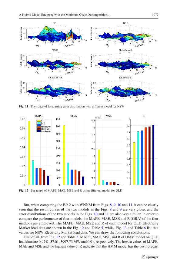
Relative absolute error is used to estimate the performance of the six forecasting models.Figures 10 and 11 have shown the relative absolute error space of four forecasting models inQLD and NSW Electricity Market data, respectively. Error space is a very complex surfacein the three-dimensional space on which the height of each point corresponds to a relativeabsolute error value; the x-axis and y-axis are the half hour of day and the day of week,

123

A Hybrid Model Equipped with the Minimum Cycle Decomposition… 1075

Fig. 7 Every sub-model’ s performance evaluation results of MAPE using HMM model for load data from25th May, 2015 to 31st May, 2015 (336 load data)

Fig. 8 Forecasted electricity load result for QLD: the solid line-black show the actual load signal, the dashedline-blue, dash-dotted line-red lines, solid line-aquamarine and solid line-yellow show the forecasted loadsignals with four models, respectively. (electricity load: MW). (Color figure online)

respectively. From the above two figures, we can draw the following conclusions. Firstly,dividing the series into 48 subseries shows the good performance than dividing the seriesinto seven groups. For short-term load forecasting, the error range [−3,+3%] is always con-sidered as a standard to measure forecasting results [45], the range is also used to comparefour methods as follows [35]. For QLD Electricity Market shown in Fig. 10, we can easilyobserve that HMM model just has less than 5% forecasting result points exceed the rangein total 336 result points. For DEEPLSSVM and DEESGRNN models, there are about 10%result points larger than 3%. In the WNNM model and BP-2 model, there are about 25%forecasting result points larger than 3%. However, the BP-1 model forecasting errors arealmost 80% exceed the range. Secondly, the values of the data pro-process and of the param-eter optimization algorithm MEC are indicated by phenomenon that the proposed HMMalgorithm has good potential than WNNM model. Thirdly, rolling forecast mechanism may

123

1076 Z. He et al.

Fig. 9 Forecasted electricity load result for NSW: the solid line-black show the actual load signal, the dashedline-blue, dash-dotted line-red lines, solid line-aquamarine and solid line-yellow show the forecasted loadsignals with four models, respectively. (electricity load: MW). (Color figure online)

Fig. 10 The space of forecasting error distribution with different model for QLD

lead to the error transfer and amplification by using forecast results to further forecasting.From the error distribution of three models BP-2, WNNM and HMM model, it can be obvi-ously found that the relative absolute error significantly increased about on the sixth and theseventh day of a week. This phenomenon mainly stems from the fact that these three modelsare adopted rolling forecast mechanism. In conclusion, the performance of the HMMmodelis better than other five contrasted models. Similar phenomenon on NSW Electricity Marketdata have been obtained as shown in Fig. 11, although all error distributions, among whichthe error of the HMM method is just about 80% in the range, are not as good as on QLDElectricity Market data.

123

A Hybrid Model Equipped with the Minimum Cycle Decomposition… 1077

Fig. 11 The space of forecasting error distribution with different model for NSW

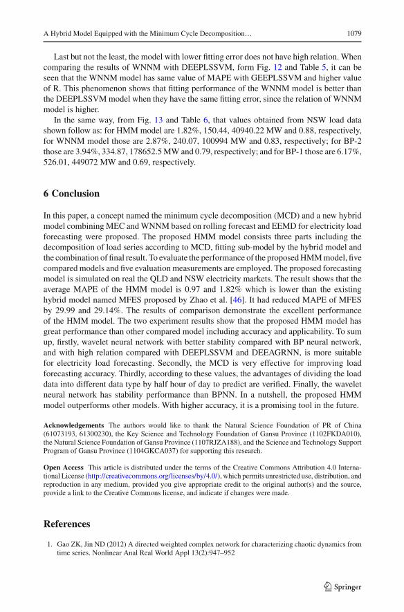
Fig. 12 Bar graph of MAPE, MAE, MSE and R using different model for QLD

But, when comparing the BP-2 with WNNM from Figs. 8, 9, 10 and 11, it can be clearlyseen that the result curves of the two models in the Figs. 8 and 9 are very close, and theerror distributions of the two models in the Figs. 10 and 11 are also very similar. In order tocompare the performance of four models, the MAPE, MAE, MSE and R (GRA) of the fourmethods are employed. The MAPE, MAE, MSE and R of each model for QLD ElectricityMarket load data are shown in the Fig. 12 and Table 5, while, Fig. 13 and Table 6 list thatvalues for NSW Electricity Market load data. We can draw the following conclusions.

First of all, from Fig. 12 and Table 5, MAPE, MAE, MSE and R of HMMmodel on QLDload data are 0.97%, 57.01, 5997.73MWand 0.91, respectively. The lowest values ofMAPE,MAE andMSE and the highest value of R indicate that the HMMmodel has the best forecast

123

1078 Z. He et al.

Table 5 Performance evaluation results of MAPE, MAE, MSE and R using different model for QLD

Performance evaluation BP-1 BP-2 WNNM DEEPLSSVM DEESGRNN HMM model

MAPE (%) 6.81% 2.57% 1.78% 1.78% 1.58% 0.97%

MAE (MW) 407.1302 151.4424 104.5034 103.3521 91.7885 57.01391

MSE (MW) 245764 31121.51 18867.2 19492.56 21841.75 5997.733

R 0.6443 0.8096 0.8237 0.8723 0.8861 0.9108

Fig. 13 Bar graph of MAPE, MAE, MSE and R using different model for NSW

Table 6 Performance evaluation results of MAPE, MAE, MSE and R using different model for NSW

Performance evaluation BP-1 BP-2 WNNM DEEPLSSVM DEESGRNN HMM model

MAPE (%) 6.17% 3.94% 2.87% 3.31% 3.21% 1.82%

MAE (MW) 526.012 334.869 240.069 274.159 262.575 150.436

MSE (MW) 449072 178652.5 100994 111560.76 103442.156 40940.22

R 0.6937 0.7901 0.8291 0.7962 0.8164 0.8841

accuracy and high curve fitting degree. Those values are seen in WNNM model are 1.78%,104.50, 1.8867.2 MW and 0.82, respectively. BP-2, by contrast, the MAPE, MAE and MSEincrease 0.97%, 46.94 and 12254.31 MW, although R value just reduce 0.014.

And then, those values of BP-1 model are 6.81%, 407.13, 245764MW and 0.644, respec-tively. The worst values of all these indicate that BP-1 makes the poorest performance amongall models. This phenomenon displays visually that the advantages, that divided the load datainto different data type according to half hour of day when forecasting, is verified.

What’smore, the following phenomenon shows that BP neural network andwavelet neuralnetwork also can be a good fitting of nonlinear functions, but wavelet neural network havebetter accuracy and faster convergence speed. It is very interesting that, compare with BP-2model in this simulation, WNNM model’s R also just increased 0.039, which is very lowcompare with 0.09(0.06) obtained fromHMMmodel andWNNM for QLD(NSW) load data.

123

A Hybrid Model Equipped with the Minimum Cycle Decomposition… 1079

Last but not the least, the model with lower fitting error does not have high relation. Whencomparing the results of WNNM with DEEPLSSVM, form Fig. 12 and Table 5, it can beseen that the WNNM model has same value of MAPE with GEEPLSSVM and higher valueof R. This phenomenon shows that fitting performance of the WNNM model is better thanthe DEEPLSSVMmodel when they have the same fitting error, since the relation of WNNMmodel is higher.

In the same way, from Fig. 13 and Table 6, that values obtained from NSW load datashown follow as: for HMMmodel are 1.82%, 150.44, 40940.22 MW and 0.88, respectively,for WNNM model those are 2.87%, 240.07, 100994 MW and 0.83, respectively; for BP-2those are 3.94%, 334.87, 178652.5MWand 0.79, respectively; and for BP-1 those are 6.17%,526.01, 449072 MW and 0.69, respectively.

6 Conclusion

In this paper, a concept named the minimum cycle decomposition (MCD) and a new hybridmodel combiningMEC andWNNM based on rolling forecast and EEMD for electricity loadforecasting were proposed. The proposed HMM model consists three parts including thedecomposition of load series according to MCD, fitting sub-model by the hybrid model andthe combination of final result. To evaluate the performance of the proposedHMMmodel, fivecompared models and five evaluation measurements are employed. The proposed forecastingmodel is simulated on real the QLD and NSW electricity markets. The result shows that theaverage MAPE of the HMM model is 0.97 and 1.82% which is lower than the existinghybrid model named MFES proposed by Zhao et al. [46]. It had reduced MAPE of MFESby 29.99 and 29.14%. The results of comparison demonstrate the excellent performanceof the HMM model. The two experiment results show that the proposed HMM model hasgreat performance than other compared model including accuracy and applicability. To sumup, firstly, wavelet neural network with better stability compared with BP neural network,and with high relation compared with DEEPLSSVM and DEEAGRNN, is more suitablefor electricity load forecasting. Secondly, the MCD is very effective for improving loadforecasting accuracy. Thirdly, according to these values, the advantages of dividing the loaddata into different data type by half hour of day to predict are verified. Finally, the waveletneural network has stability performance than BPNN. In a nutshell, the proposed HMMmodel outperforms other models. With higher accuracy, it is a promising tool in the future.

Acknowledgements The authors would like to thank the Natural Science Foundation of PR of China(61073193, 61300230), the Key Science and Technology Foundation of Gansu Province (1102FKDA010),the Natural Science Foundation of Gansu Province (1107RJZA188), and the Science and Technology SupportProgram of Gansu Province (1104GKCA037) for supporting this research.

Open Access This article is distributed under the terms of the Creative Commons Attribution 4.0 Interna-tional License (http://creativecommons.org/licenses/by/4.0/), which permits unrestricted use, distribution, andreproduction in any medium, provided you give appropriate credit to the original author(s) and the source,provide a link to the Creative Commons license, and indicate if changes were made.

References

1. Gao ZK, Jin ND (2012) A directed weighted complex network for characterizing chaotic dynamics fromtime series. Nonlinear Anal Real World Appl 13(2):947–952

123

1080 Z. He et al.

2. GaoZKet al (2015)Multivariateweighted complex network analysis for characterizing nonlinear dynamicbehavior in two-phase flow. Exp Therm Fluid Sci 60:157–164

3. Gao ZK et al (2016) Characterizing slug to churn flow transition by using multivariate pseudo Wignerdistribution and multivariate multiscale entropy. Chem Eng J 291:74–81

4. Gao Z-K, Small M, Kurths J (2017) Complex network analysis of time series. EPL (Europhysics Letters)116(5):50001

5. Gao Z et al (2016) A four-sector conductance method for measuring and characterizing low-velocityoil-water two-phase flows. IEEE Trans Instrum Meas 65(7):1690–1697

6. Ranjan M, Jain VK (1999) Modelling of electrical energy consumption in Delhi. Energy 24(24):351–3617. Papadakis SE et al (1995) A novel approach to short-term load forecasting using fuzzy neural networks.

IEEE Trans Power Syst 13(2):1518–15248. Deng JL (1982) Control problems of grey system. Syst Control Lett 1(5):288–2949. Hamzacebi C, Es HA (2014) Forecasting the annual electricity consumption of Turkey using an optimized

grey model. Energy 70(3):165–17110. Zhou P, Ang BW, Poh KL (2006) A trigonometric grey prediction approach to forecasting electricity

demand. Energy 31(14):2839–284711. Jin M et al (2012) Short-term power load forecasting using grey correlation contest modeling. Expert

Syst Appl Int J 39(1):773–77912. Al-Hamadi HM, Soliman SA (2004) Short-term electric load forecasting based on Kalman filtering

algorithm with moving window weather and load model. Electr Power Syst Res 68(1):47–5913. Tan Z et al (2010)Day-ahead electricity price forecasting usingwavelet transform combinedwithARIMA

and GARCH models. Appl Energy 87(11):3606–361014. Pappas SS et al (2008) Electricity demand loads modeling using AutoRegressive Moving Average

(ARMA) models. Energy 33(9):1353–136015. Contreras J et al (2002) ARIMA models to predict next-day electricity prices. IEEE Power Eng Rev

22(9):57–5716. Geng WH, Sun Q, Xing-Yuan LI (2006) Short-term load forecasting based on compensated fuzzy neural

networks and linear models. Power Syst Technol 30(23):1–517. Trapero JR, Kourentzes N, Martin A (2015) Short-term solar irradiation forecasting based on Dynamic

Harmonic Regression. Energy 84:289–29518. Garcia RC et al (2005) A GARCH forecasting model to predict day-ahead electricity prices. IEEE Trans

Power Syst 20(2):867–87419. AmjadyN (2001) Short-termhourly load forecasting using time-seriesmodelingwith peak load estimation

capability. IEEE Trans Power Syst 16(3):498–50520. Rahman S, Hazim O (1996) Load forecasting for multiple sites: development of an expert system-based

technique. Electr Power Syst Res 39(39):161–16921. Hu W et al (2016) A short-term traffic flow forecasting method based on the hybrid PSO-SVR. Neural

Process Lett 43(1):155–17222. ShiD et al (2007) Product demand forecastingwith a novel fuzzyCMAC.Neural Process Lett 25(1):63–7823. Mez-Gil P et al (2011) A neural network scheme for long-term forecasting of chaotic time series. Neural

Process Lett 33(3):215–23324. Ferreira TA, Vasconcelos GC, Adeodato PJ (2008) A new intelligent system methodology for time series

forecasting with artificial neural networks. Neural Process Lett 28(2):113–12925. Xiao L et al (2015) A combined model based on data pre-analysis and weight coefficients optimization

for electrical load forecasting. Energy 82:524–54926. Wang J et al (2010) Combined modeling for electric load forecasting with adaptive particle swarm

optimization. Energy 35(4):1671–167827. Osório GJ, Matias JCO, Catalão JPS (2014) Electricity prices forecasting by a hybrid evolutionary-

adaptive methodology. Energy Conver Manag 80(80):363–37328. Chen Y et al (2015) A hybrid application algorithm based on the support vector machine and artificial

intelligence: an example of electric load forecasting. Appl Math Model 39(9):2617–263229. Pati YC et al (1988) Neural networks & tactile imaging. Neural Netw 1:45930. Zhang Q, Benveniste A (1992) Wavelet networks. IEEE Trans Neural Netw 3(6):889–89831. Gao R, Tsoukalas LH (2001) Neural-wavelet methodology for load forecasting. J Intell Robot Syst

31(1):149–15732. UlagammaiM et al (2007) Application of bacterial foraging technique trained artificial andwavelet neural

networks in load forecasting. Neurocomputing 70(16–18):2659–266733. Wang J et al (2011) Chaotic time series method combined with particle swarm optimization and trend

adjustment for electricity demand forecasting. Expert Syst Appl 38(7):8419–8429

123

A Hybrid Model Equipped with the Minimum Cycle Decomposition… 1081

34. Yang X et al (2010) An improved WM method based on PSO for electric load forecasting. Expert SystAppl 37(12):8036–8041

35. Wang J et al (2012) An annual load forecasting model based on support vector regression with differentialevolution algorithm. Appl Energy 94(6):65–70

36. Wang Z et al (2015) Fine-scale estimation of carbon monoxide and fine particulate matter concentrationsin proximity to a road intersection by usingwavelet neural networkwith genetic algorithm.Atmos Environ104:264–272

37. ZhaoW,Wang J, Lu H (2014) Combining forecasts of electricity consumption in China with time-varyingweights updated by a high-order Markov chain model. Omega 45(45):80–91

38. Huang CM, Yang HT (2001) Evolving wavelet-based networks for short-term load forecasting. IEE ProcGener Transm Distrib 148(3):222–228

39. Sun C, Sun Y, Xie K (2000) Mind-evolution-based machine learning: an efficient approach of evolutioncomputation. In: Proceedings of the world congress on intelligent control and automation, 2000.

40. WIKIPEDIA Web Site [Online]. National Electricity Market. https://en.wikipedia.org/wiki/National_Electricity_Market

41. HuangNE,WuZ (2008)A review onHilbert-Huang transform:method and its applications to geophysicalstudies. Rev Geophys 46(2):2008

42. Wu Z, HuangNE (2011) Ensemble empirical mode decomposition: a noise-assisted data analysis method.Adv Adapt Data Anal 1(1):1–41

43. Jie J, Zeng J, Han C (2007) An extended mind evolutionary computation model for optimizations. ApplMath Comput 185(2):1038–1049

44. Wu H (2002) A comparative study of using grey relational analysis in multiple attribute decision makingproblems. Qual Eng 15(15):209–217

45. Niu D, Wang Y, Wu DD (2010) Power load forecasting using support vector machine and ant colonyoptimization. Expert Syst Appl 37(3):2531–2539

46. An N et al (2013) Using multi-output feedforward neural network with empirical mode decompositionbased signal filtering for electricity demand forecasting. Energy 49(1):279–288

123