Embed Size (px)
Citation preview
A Hybrid Genetic Algorithm and
Evolutionary Strategy to
Automatically Generate Test Data for
Dynamic, White-Box Testing
By: Ashwin Panchapakesan
A thesis submitted to the
Faculty of Graduate and Postdoctoral Studies
In partial fulfillment of the requirements for the degree of
Master of Science in Computer Science
Ottawa-Carleton Institute for Electrical and Computer Science
School of Electrical Engineering and Computer Science
University of Ottawa
August 2013
c•Ashwin Panchapakesan, Ottawa, Canada, 2013

To Skynet. May we build it and teach it not to kill us all.
Abstract
Software testing is an important and time consuming part of the software develop-
ment cycle. While automated testing frameworks do help in reducing the amount of
programmer time that testing requires, the onus is still upon the programmer to pro-
vide such a framework with the inputs upon which the software must be tested. This
requires static analysis of the source code, which is more e�ective when performed
as a peer review exercise and is highly dependent on the skills of the programmers
performing the analysis. It also demands the allocation of precious time for those
very highly skilled programmers. An algorithm that automatically generates inputs
to satisfy test coverage criteria for the software being tested would therefore be quite
valuable, as it would imply that the programmer no longer needs to analyze code to
generate the relevant test cases. This thesis explores a hybrid evolutionary strategy
with an evolutionary algorithm to discover such test cases , in an improvement over
previous methods which overly focus their search without maintaining the diversity
required to cover the entire search space e�ciently.
3

Acknowledgments
This thesis would not have been possible if not for the e�orts of
• Dr. Panchanathan, for guiding and advising me when the answer wasn’t clear
• Dr. Petriu, for funding me and guiding my academic path, for providing me
the computational power that I needed
• Dr. Abielmona, for guiding my academic growth and learning, and for teaching
me how to be a good researcher
• Phillip Curtis, for helping me get the path generator online
• Tapan Oza for helping me draw so many graphs and brainstorm ideas for data
representation
• My parents for always being there, for their moral support and for making sure
I don’t crash, for forcing me to take breaks; the list goes on
• My grandparents for making me warm dinner every night
• My friends (the list is far too long) for letting me vent my frustrations on bad
days; for making me smile when the going was tough; for taking me out when I
needed a break; for showing me I could be clever when I thought I wasn’t and
for helping me see how clever I really wasn’t when I thought I was
• My cousins, for the unlimited supply of mokkais that got me through the di�cult
days
• Ramu, for teaching me critical thinking at an early age with his water bottle
filling methodology
4

Contents
Abstract 3
Acknowledgments 4
1. Introduction 7
1.1. Motivation . . . . . . . . . . . . . . . . . . . . . . . . . . . . . . . . . 7
1.2. Software Complexity . . . . . . . . . . . . . . . . . . . . . . . . . . . 8
1.3. Eliminating the Need for Testing . . . . . . . . . . . . . . . . . . . . 8
1.4. Automating the Process of Testing . . . . . . . . . . . . . . . . . . . 9
1.5. Thesis Contribution . . . . . . . . . . . . . . . . . . . . . . . . . . . . 9
1.6. Thesis Organization . . . . . . . . . . . . . . . . . . . . . . . . . . . . 10
2. Software Testing Methodology Overview 11
2.1. Overview . . . . . . . . . . . . . . . . . . . . . . . . . . . . . . . . . . 11
2.2. Static Software Testing . . . . . . . . . . . . . . . . . . . . . . . . . . 11
2.3. Dynamic Software Testing . . . . . . . . . . . . . . . . . . . . . . . . 12
2.4. Black Box Testing . . . . . . . . . . . . . . . . . . . . . . . . . . . . . 12
2.5. White Box Testing . . . . . . . . . . . . . . . . . . . . . . . . . . . . 13
2.5.1. Overview . . . . . . . . . . . . . . . . . . . . . . . . . . . . . 13
2.6. Path Coverage . . . . . . . . . . . . . . . . . . . . . . . . . . . . . . . 13
2.7. Summary . . . . . . . . . . . . . . . . . . . . . . . . . . . . . . . . . 14
3. Related Work 15
3.1. Overview . . . . . . . . . . . . . . . . . . . . . . . . . . . . . . . . . . 15
i
3.2. One For All (OFA) . . . . . . . . . . . . . . . . . . . . . . . . . . . . 26
3.3. One For Each (OFE) . . . . . . . . . . . . . . . . . . . . . . . . . . . 28
3.4. Summary . . . . . . . . . . . . . . . . . . . . . . . . . . . . . . . . . 28
4. Implementation 29
4.1. Overview . . . . . . . . . . . . . . . . . . . . . . . . . . . . . . . . . . 29
4.2. Workflow . . . . . . . . . . . . . . . . . . . . . . . . . . . . . . . . . 31
4.3. Algorithm Overview . . . . . . . . . . . . . . . . . . . . . . . . . . . 32
4.4. Binning, Seed Finding and Similarity Computation Algorithms . . . . 34
4.5. Detailed Algorithm Design . . . . . . . . . . . . . . . . . . . . . . . . 34
4.5.1. An Individual . . . . . . . . . . . . . . . . . . . . . . . . . . . 34
4.5.2. Population Initialization . . . . . . . . . . . . . . . . . . . . . 35
4.5.3. Computing the Fitness of an Individual . . . . . . . . . . . . . 36
4.5.4. Selecting Individuals for Mating . . . . . . . . . . . . . . . . . 36
4.5.5. Crossover . . . . . . . . . . . . . . . . . . . . . . . . . . . . . 36
4.5.6. Mutation . . . . . . . . . . . . . . . . . . . . . . . . . . . . . 37
4.5.7. Spawning . . . . . . . . . . . . . . . . . . . . . . . . . . . . . 37
4.5.8. Termination . . . . . . . . . . . . . . . . . . . . . . . . . . . . 37
4.6. Implementation Parameters . . . . . . . . . . . . . . . . . . . . . . . 37
4.7. The Pyvolution Software Package . . . . . . . . . . . . . . . . . . . . 38
4.7.1. Previous Work . . . . . . . . . . . . . . . . . . . . . . . . . . 38
4.7.2. An Example: A Genetic Algorithm to solve the Traveling Sales-
man Problem . . . . . . . . . . . . . . . . . . . . . . . . . . . 38
4.7.3. Introducing Design by Contract . . . . . . . . . . . . . . . . . 41
4.7.4. A DbC Framework for Python . . . . . . . . . . . . . . . . . . 42
4.8. Summary . . . . . . . . . . . . . . . . . . . . . . . . . . . . . . . . . 46
5. Parametric Analysis and Discussion 58
5.1. The Benchmark SUTs . . . . . . . . . . . . . . . . . . . . . . . . . . 58
ii
5.2. Experimental Data . . . . . . . . . . . . . . . . . . . . . . . . . . . . 59
5.2.1. Selecting the Best Parameters for the Hybrid Algorithm . . . 60
5.3. Properties of the Hybrid Algorithm . . . . . . . . . . . . . . . . . . . 63
5.3.1. Fewer Fitness Evaluations . . . . . . . . . . . . . . . . . . . . 63
5.3.2. Local Optima . . . . . . . . . . . . . . . . . . . . . . . . . . . 63
5.3.3. Parallelizability . . . . . . . . . . . . . . . . . . . . . . . . . . 64
5.3.4. Inability to Stop Early . . . . . . . . . . . . . . . . . . . . . . 65
5.3.5. SUT Structure . . . . . . . . . . . . . . . . . . . . . . . . . . 65
5.4. A Real World SUT . . . . . . . . . . . . . . . . . . . . . . . . . . . . 66
5.5. Summary . . . . . . . . . . . . . . . . . . . . . . . . . . . . . . . . . 67
6. Conclusions and Future Work 76
6.1. Overview . . . . . . . . . . . . . . . . . . . . . . . . . . . . . . . . . . 76
6.2. Summary of Contributions . . . . . . . . . . . . . . . . . . . . . . . . 76
6.3. Future Work . . . . . . . . . . . . . . . . . . . . . . . . . . . . . . . . 77
Appendix A. The CFG Package 79
A.1. Motivation . . . . . . . . . . . . . . . . . . . . . . . . . . . . . . . . . 79
A.2. Overview . . . . . . . . . . . . . . . . . . . . . . . . . . . . . . . . . . 79
A.3. Source-code to XML . . . . . . . . . . . . . . . . . . . . . . . . . . . 80
Appendix B. Dynamic White Box Testing 85
B.1. Overview . . . . . . . . . . . . . . . . . . . . . . . . . . . . . . . . . . 85
B.2. Node or Statement Coverage . . . . . . . . . . . . . . . . . . . . . . . 85
B.3. Edge Coverage . . . . . . . . . . . . . . . . . . . . . . . . . . . . . . 87
B.4. Condition Coverage . . . . . . . . . . . . . . . . . . . . . . . . . . . . 88
B.5. Path Coverage . . . . . . . . . . . . . . . . . . . . . . . . . . . . . . . 88
Appendix C. Evolutionary Algorithms 89
C.1. Genetic Algorithms . . . . . . . . . . . . . . . . . . . . . . . . . . . . 89
C.1.1. Overview . . . . . . . . . . . . . . . . . . . . . . . . . . . . . 89
iii
C.1.2. Chromosome . . . . . . . . . . . . . . . . . . . . . . . . . . . 90
C.1.3. Individual . . . . . . . . . . . . . . . . . . . . . . . . . . . . . 90
C.1.4. Population Generation . . . . . . . . . . . . . . . . . . . . . . 90
C.1.5. Fitness . . . . . . . . . . . . . . . . . . . . . . . . . . . . . . . 91
C.1.6. Selection . . . . . . . . . . . . . . . . . . . . . . . . . . . . . . 91
C.1.7. Biased Roulette Wheel Selection . . . . . . . . . . . . . . . . . 92
C.1.8. Tournament Selection . . . . . . . . . . . . . . . . . . . . . . . 92
C.1.9. Crossover . . . . . . . . . . . . . . . . . . . . . . . . . . . . . 93
C.1.10. Mutation . . . . . . . . . . . . . . . . . . . . . . . . . . . . . 94
C.2. Evolutionary Strategy . . . . . . . . . . . . . . . . . . . . . . . . . . 95
Bibliography 96
iv
List of Algorithms
3.1. Algorithm to Demonstrate Deviation and Violation . . . . . . . . . . 20
4.1. Finding the Parent Scope of a Scope in the SUT . . . . . . . . . . . . 31
4.2. Computing the Nested Scopes of a List of all Scopes in the SUT . . . 32
4.3. Path Generator’s Helper Function . . . . . . . . . . . . . . . . . . . . 49
4.4. The Path Generator Algorithm . . . . . . . . . . . . . . . . . . . . . 50
4.5. Classifying Target Paths into Bins . . . . . . . . . . . . . . . . . . . . 51
4.6. Computing Relative Similarities among Paths . . . . . . . . . . . . . 53
4.7. Computing Absolute Similarities among Paths . . . . . . . . . . . . . 54
4.8. Computing Similarity Matrix . . . . . . . . . . . . . . . . . . . . . . 54
4.9. Computing the Seed Individual of a Bin of Target Paths . . . . . . . 55
4.10. Contracts for a Matrix Multiplication Function in PyContract . . . . 55
4.11. Contracts for the Crossover function for the Traveling Salesman Problem 57
4.12. Contracts for the Crossover function for the Traveling Salesman Problem 57
5.1. The Triangle Classification Algorithm . . . . . . . . . . . . . . . . . 58
5.2. The Bubble-Sort Algorithm . . . . . . . . . . . . . . . . . . . . . . . 60
5.3. The Simplex Algorithm . . . . . . . . . . . . . . . . . . . . . . . . . 62
5.4. The Hu�man Tree Maker . . . . . . . . . . . . . . . . . . . . . . . . . 67
5.5. The Helper Function to encode . . . . . . . . . . . . . . . . . . . . . 67
5.6. The Encoding Function . . . . . . . . . . . . . . . . . . . . . . . . . . 68
5.7. Main . . . . . . . . . . . . . . . . . . . . . . . . . . . . . . . . . . . . 68
A.1. A Simple Python SUT . . . . . . . . . . . . . . . . . . . . . . . . . . 80
1

A.2. Converting Fig. A.3 to a CFG . . . . . . . . . . . . . . . . . . . . . . 84
B.1. A Simple Program . . . . . . . . . . . . . . . . . . . . . . . . . . . . 86
2
List of Figures
3.1. An Example of the Chromosome Representation Used in [1] . . . . . 15
3.2. CFG for Algorithm 3.1 . . . . . . . . . . . . . . . . . . . . . . . . . . 20
3.3. Progression of a GA Demonstrating Ine�cient Convergence in the OFA
Paradigm . . . . . . . . . . . . . . . . . . . . . . . . . . . . . . . . . 27
4.5. Example Chromosome for Input Vector <3,4,5> . . . . . . . . . . . . 35
4.1. Full Process Workflow . . . . . . . . . . . . . . . . . . . . . . . . . . 48
4.2. Initialization and Seeded ES Algorithm . . . . . . . . . . . . . . . . 51
4.3. The SeededGA Algorithm . . . . . . . . . . . . . . . . . . . . . . . . 52
4.4. Process flow of Recursive Binning and Seed Finding . . . . . . . . . . 53
4.6. Creating a Single Individual Encoding 3 Input Variables . . . . . . . 56
4.7. Generating the Initial Population . . . . . . . . . . . . . . . . . . . . 56
4.8. Computing the Fitness of an Individual Against a Specific Target Path 57
5.1. The CFG of Algorithm 5.1 . . . . . . . . . . . . . . . . . . . . . . . . 59
5.2. The CFG of Algorithm 5.2 . . . . . . . . . . . . . . . . . . . . . . . . 61
5.3. The CFG of Algorithm 5.3 . . . . . . . . . . . . . . . . . . . . . . . . 69
5.4. The E�ects of Threshold Parameters on the Hybrid . . . . . . . . . . 70
5.5. Performance of Each Parameter Set on Each SUT . . . . . . . . . . . 71
5.6. Comparing Hybrid with OFA and OFE . . . . . . . . . . . . . . . . . 72
5.7. Process flow of Recursive Binning and Seed Finding . . . . . . . . . . 73
5.8. CFG of Algorithm 5.7 . . . . . . . . . . . . . . . . . . . . . . . . . . 74
5.9. Performance Metrics on the Hu�man Encoder . . . . . . . . . . . . . 75
3

A.1. Converting Source-code to CFG . . . . . . . . . . . . . . . . . . . . . 80
A.2. The AST of Algorithm A.1 . . . . . . . . . . . . . . . . . . . . . . . . 82
A.3. The XML Derived from Fig. A.2 . . . . . . . . . . . . . . . . . . . . . 83
A.4. The CFG Generated from Fig. A.3 . . . . . . . . . . . . . . . . . . . 83
B.1. CFG for the SUT Presented in Algorithm B.1 . . . . . . . . . . . . . 86
C.1. Example Chromosome for Input Vector <3,4,5> . . . . . . . . . . . 90
C.2. Tri-Chromosome Individual for Input Vector <3,4,5> . . . . . . . . 90
C.3. Uniform Crossover Example . . . . . . . . . . . . . . . . . . . . . . . 94
C.4. Possible Child of One-Point Crossover . . . . . . . . . . . . . . . . . 94
C.5. Possible Mutation . . . . . . . . . . . . . . . . . . . . . . . . . . . . 95
4
List of Tables
0.1. List of Abbreviations . . . . . . . . . . . . . . . . . . . . . . . . . . . 6
3.1. Degree of Match Between Two Paths Based on Path Predicates . . . 18
3.2. Target and Induced Paths for Algorithm 3.1 . . . . . . . . . . . . . . 21
4.1. Experimental Parameters . . . . . . . . . . . . . . . . . . . . . . . . . 38
4.2. Explanations of Contracts in Algorithm 4.11 . . . . . . . . . . . . . . 44
5.1. Identifying Parameter Sets, SUTs, and Algorithms . . . . . . . . . . . 60
B.1. Specification for AlgorithmAlgorithm B.1 . . . . . . . . . . . . . . . . 86
B.2. Node-Statement Representation . . . . . . . . . . . . . . . . . . . . . 87
B.3. Inputs for Node Coverage . . . . . . . . . . . . . . . . . . . . . . . . 87
C.1. Relative Fitness of Individuals in a Population . . . . . . . . . . . . 92
C.2. A Biased Roulette-Wheel for the Individuals in Table Tab. C.1 . . . 92
5

List of Abbreviations
AST Abstract Syntax TreeCFG Control Flow GraphDbC Design by ContractEA Evolutionary AlgorithmES Evolutionary StrategyGA Genetic AlgorithmOFA One For AllOFE One For EachSUT Software Under Test
Table 0.1.: List of Abbreviations
6

1. Introduction
1.1. Motivation
Any software, as part of the development process, needs to be tested before it is
deployed. This is becoming more and more relevant in today’s world, given how
many critical systems are controlled by software. A bug in mission critical software
could have severe and dire consequences, including the loss of equipment and possibly
human life (as in the case of medical software, flight control software, mission critical
rocket propulsion systems [2], etc) . As a result, it is imperative that software be
thoroughly tested before it is deployed.
The testing process consumes approximately 50% of the software development time-
line [3]. Considering how expensive it is to develop software, it is clear that reducing
the amount of time spent on testing the SUT (Software Under Test) would lead
to an optimization of the time spent in the development process and therefore an
optimization in the cost of producing software. This reduction in time may possibly
come from any of the following avenues:
1. Producing software that is less complex
2. Producing software that is initially bug free, thus eliminating the need for testing
3. Automating the process of testing
7
1.2 Software Complexity
1.2. Software Complexity
It is clear that software has been increasing in complexity with time. This is easily
observable from the evolution of computer programs from punch cards to modern
software with applications in auto-pilot systems, security (both electronically and
physically, as in building security systems) and even health care systems.
Further, with advances in computational intelligence and in methodologies employed
in producing hardware and the capabilities of hardware itself, it is clear that the
complexity of modern software will only increase over time. Therefore, it is irrational
to expect reductions in the required time to test software from a decrease in the
complexity of modern software.
1.3. Eliminating the Need for Testing
Since software is architected and developed by human beings, it is almost impossible
to expect a programmer to code a full specification correctly on the first attempt,
without any debugging. This problem is only exasperated when one considers that
most modern software is written by teams of programmers, communicating amongst
themselves. Owing to errors in communication, it is even less rational to expect
software collaboratively authored by such teams to be bug-free in the first release
without proper testing. Even with theoretic proofs of code, there is no guarantee that
there are no bugs in the software. Indeed, there is no guarantee that the developed
software even accurately implements the specification that it was supposed to. This
is one of the motivations behind black-box testing, or specification based testing
(discussed further in sec. 2.4) [4]. Thus, it is unlikely that any optimization in SUT
testing time can be achieved from eliminating the need for testing.
8
1.4 Automating the Process of Testing
1.4. Automating the Process of Testing
From the discussion in sec. 1.2 and sec. 1.3, it is clear that the only remaining method
of optimizing the time spent on the testing process is to automate the software testing
process itself. Testing the SUT requires that the agent performing the tests (whether
that agent is human or a computer program) provides the software with some inputs
and compares them against the expected behavior. If the SUT behaves as expected,
it passes the test, else it fails the test. While the running of the tests themselves can
be executed by automated testing frameworks[5], it is the generation of input data,
that is included in the test cases, that seems to require human input and resources.
It is the generation of such test case data that is of most interest in this thesis.
1.5. Thesis Contribution
This thesis uses evolutionary algorithms to generate inputs with which to test soft-
ware. Further, it explores problems faced by genetic algorithms arising from unfavor-
able initial conditions and attempts to mitigate the e�ects of these problems with a
hybrid evolutionary algorithm (composed of an Evolutionary Strategy and a Genetic
Algorithm) to find better initialization conditions for the Genetic Algorithm. Thus,
the Genetic Algorithm is able to better generate inputs with which to test the soft-
ware at hand. It is important to note that the work presented in this thesis is only
applicable to software that compiles cleanly and does not contain syntax errors; only
the semantics of the software are tested to determine if the implementation of the
software is faithful to the specification of which it claims to be an implementation.
Thus, the contributions of this thesis can be summarized as:
1. Generate inputs with which to test the given software
• Perform this generation of inputs faster than the current state of the art
• Search the space of test-input more thoroughly than the current state of
the art
9

1.6 Thesis Organization
2. Find more appropriate initialization conditions for the Genetic Algorithms used
to solve the above objective
• Provide a mechanism for the Genetic Algorithm to learn better initializa-
tion conditions over time, so that it may discover the inputs with which to
test the software, faster than the current state of the art
1.6. Thesis Organization
The remainder of this thesis is organized as follows. chapter 2 introduces the dif-
ferent types of software testing and highlights the paradigm that will be studied in
this thesis. Further, it contains a brief introduction to the two classes of evolution-
ary algorithms used in this thesis. Next, chapter 3 contains a survey of the use of
genetic algorithms in software testing, classifying them into the two main paradigms
against which the hybrid algorithm presented in this thesis will be compared. Finally,
chapter 4 discusses the implementation of the hybrid algorithm in detail, including
all parametric settings and software packages used. The analysis on the e�ects of
these parameters is shown in chapter 5 and chapter 6 discusses the limitations and
future directions of this thesis.
10

2. Software Testing Methodology
Overview
2.1. Overview
Software testing can be broadly categorized into static and dynamic testing, explained
in the following subsections.
2.2. Static Software Testing
Under the static testing paradigm, a code reviewer (e.g. a human) performs code
reviews and walkthroughs of the SUT with hypothetical inputs, visually following
the logical program flow. This is highly dependent on the skill of the reviewer and
requires a lot of the reviewer’s time [6, 7].
Further improvements in static testing allowed code to be symbolically analyzed,
collecting predicates for the various paths of execution of the code. From these
predicates, it is determined which paths may be infeasible or erroneous [8]. Others
have used such an approach and combined these predicates with a constraint solver
to determine which paths may be infeasible in a SUT [9].
11
2.3 Dynamic Software Testing
2.3. Dynamic Software Testing
On the other hand, under the dynamic testing paradigm, the code for the SUT is
actually run with the given test inputs. The behavior of the SUT is observed and
compared against its expected behavior and the test passes or fails depending on
whether the observed behavior matches the expected behavior.
As outlined in [10], Dynamic testing can be split into two categories:
Black Box Testing also known as functional testing; tests the SUT to ensure that it
is faithful to the specifications from which it was authored;
White Box Testing also known as structural testing; tests the SUT to attain some
level of code coverage and to test it on boundary conditions, etc (to be discussed
further in sec. 2.5).
2.4. Black Box Testing
The purpose of black box testing is to ensure that the classes and functions in the
SUT are indeed correct implementations of the specification, based on which they
were developed [10]. As such, test cases for Black Box Testing are generally com-
posed of input/output pairs; a SUT passes a test case if it produces the expected
output, when run on the given input. Thus, this testing paradigm provides a test-
ing methodology to ensure that the implemented functions and classes are indeed a
correct implementation of the specification of the SUT (i.e. functional testing).
Note that in this paradigm, the source code is not necessarily available to the tester,
as a result of which, it can not be tested for the presence of code bloat, inexecutable
code, etc.
12
2.5 White Box Testing
2.5. White Box Testing
White box testing, also known as structural testing, aims to test code coverage and
edge cases. It is generally accepted for this purpose that “code coverage” means
“covering su�ciently many paths of execution”. Using path coverage as a heuristic,
it is possible to determine the existence of paths in source-code that may not be
executable. Further, once su�cient path coverage has been achieved, the SUT is
declared to be adequately tested and any test cases not covered by the automated
testing process are done so by a human agent.
This is still an improvement, as the test cases automated by the test case generator
would have otherwise been generated by a human agent as well.
2.5.1. Overview
White box testing is a software testing paradigm that uses the source code of the SUT
to test it. It is used to ensure that all parts of the code’s structure are executable -
to ensure code coverage1. As such, there are several forms of white-box testing2. In
each form, the SUT is converted into a control flow graph (CFG) - a mathematical
representation of the logical program flow of the SUT. In a CFG, each statement
is a node and sequential statements are connected by edges. Branching statements
(if-then-else statements, for-loops and while-loops) are characterized by mul-
tiple outgoing edges from a node, with conditions on each edge.
2.6. Path Coverage
Path coverage is one of the stronger testing criteria3, and is widely accepted as a
natural criterion of program testing completeness [8]. It requires that every path in
the CFG be executed at least once by the test suite. This is true despite the fact1seee sec. 2.6 for mo2see B for more3See for background information on the di�erent forms of coverage in white-box testing
13

2.7 Summary
that the presented test suite satisfies this criterion . As a result, this thesis focuses
on generating input vectors that satisfy path coverage. It is left to the tester of the
software to determine what percentage of all paths in the CFG need to be induced
by the inputs generated by the work presented in this thesis.
2.7. Summary
It is clear that Path Coverage is the strongest criterion with which to perform software
testing. It requires the generation of a CFG from the source code of the SUT, and a
threshold (set by the tester) for the minimum percentage of paths to be covered by
the test suite. This thesis focusses on generating input vectors that satisfy the path
coverage criterion to test SUTs.
14
3. Related Work
3.1. Overview
Jones et. al. [1] use a GA to structurally test software. They use single-chromosome
individuals that encode test values for all input variables. For example, a population
of S individuals represents S test cases for the SUT; each individual encodes a test
value for each of the input variables in a segment of the chromosome. Thus, for a
program with N input variables, there are qN
i=0 ni
bits in a chromosome encoding
test values for it, where ni
is the number of bits required to encode a test value for
the ith input variable. An example representation of the input vector <3,1> is shown
in Figure Fig. 3.1.
Such a GA is analogous to one that uses S individuals with N chromosomes each 1.
Input Variable 1 Input Variable 2
1 0 1 0 1
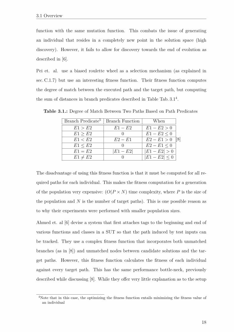
Figure 3.1.: An Example of the Chromosome Representation Used in [1]
Jones et. al. use the reciprocal of the minimum absolute di�erence between the
generated and required values for variables in path predicates as the fitness function
of an individual. For example, if a path predicate requires that variables A and B are
equal (i.e. A == B), then the fitness function would calculate 1|A≠B|
2, using appropriate
guards to ensure that division-by-zero cases are appropriately handled. If this GA1of course, in such a GA, crossover and mutation operators will need to be modified slightly to
accommodate the di�erence in representation. These are explained further, when analyzing thepresented reproduction operations
2Similarly, if a path predicate requires A>B, then the fitness function would calculate 1|A≠B|+1
15
3.1 Overview
were modeled with multi-chromosome individuals, then two chromosomes would be
required - one each for the variables A and B. Such semantic analysis is beyond the
scope of the work presented in this thesis, as a result of which the fitness function
used therein does not perform such semantic analysis3.
In addition, Jones et. al. define a uniform crossover function (as described in
sec. C.1.9.1). This is analogous to performing two uniform crossovers with each of
the two corresponding pairs of chromosomes in a GA using two-chromosome indi-
viduals. However, such a crossover function may move the GA to a completely new
point in the solution space, and not create an individual that resides part way be-
tween the parents as is typically expected of GAs. Still, this has the advantage of
escaping local optima with higher probability, especially towards the end of evolution
(where one-point crossovers are unable to make a meaningful contribution due to
the low probability of a one-point crossover producing an o�spring that can escape a
particular local optimum).
It is interesting to note that Jones et. al. use a mutation function that flips each bit
in a chromosome with probability 1qN
i=0 ni. This implies that it is likely that exactly
one bit per chromosome will be flipped as a result of this mutation operator. This
can be viewed as the alteration of one random bit in the encoding of the value of one
of the input variables. While it is reasonable to use this mutation operation, using
a mutation operation that flips a random bit in the encoding of each variable should
also be explored. Such a mutation operation would allow the GA to escape local
optima more quickly by generating mutants that are not constrained to any values
along any axes in the search space (as would be the case if only one bit was mutated).
Jones et. al. were able to overcome this limitation by mutating the most and least
significant bits with higher probability than the rest of the bits in the chromosome.
Also, the GA that they used extremely favored diversity, so that each individual in
each generation of the population was unique. This is to say that in any generation
of the population, there were no two individuals that encoded the same test inputs.
3The actual fitness function used is defined in sec. 4.5.3
16
3.1 Overview
While this is one way to force the GA to discover inputs that satisfied more paths in
the CFG, it is also likely to generate illegal inputs. Indeed, this is one of the problems
that Jones et. al. acknowledge and explicitly do not solve. As a result of ignoring
this problem, it is likely that a larger than desirable fraction of the population would
traverse the same path on the CFG. Since this is undesirable, a GA that is used to
generate test input data should address this problem by not generating too many
individuals that traverse the same path on the CFG.
Further, biasing the GA to this degree, towards diversity has the additional conse-
quence of slowing down the runtime, as each individual (either generated randomly
for the initial population or as a result of reproduction operations) must be checked
for pre-existing doppelgangers (i.e. individuals in the population that are identical to
and were generation prior to the currently generated individual) in the population.
On the other hand, Pei et. al. note that generating inputs to cover all possible paths
in the CFG of a SUT is sometimes intractable and as a result, paths need to be
selected for adequate coverage [8]. This can be achieved in one of two ways:
1. a human agent provides a list of paths that need to be covered for adequate test
coverage; or
2. paths are classified into several bins and a human-selected path from each bin
needs to be covered in order to satisfy coverage
(item 1) is counter intuitive to the purpose of automation. Since there are automated
methods of generating CFGs [11] and computing the similarity between pairs of paths
within a CFG [12], it seems that selecting appropriate paths for adequate test coverage
should be automated, as part of automating the testing of the SUT. However, since
this technology was not available at the time, Pei et. al. employ user-provided paths
to test the individuals of their GA.
Similarly, (item 2) is also counter intuitive to the idea of automation, since it is
possible to task a GA with generating inputs to cover all paths in a group [6, 12].
Pei et. al. use the same encoding scheme as in [1], but use a single point crossover
17
3.1 Overview
function with the same mutation function. This combats the issue of generating
an individual that resides in a completely new point in the solution space (high
discovery). However, it fails to allow for discovery towards the end of evolution as
described in [6].
Pei et. al. use a biased roulette wheel as a selection mechanism (as explained in
sec. C.1.7) but use an interesting fitness function. Their fitness function computes
the degree of match between the executed path and the target path, but computing
the sum of distances in branch predicates described in Table Tab. 3.14.
Table 3.1.: Degree of Match Between Two Paths Based on Path Predicates
Branch Predicate5 Branch Function WhenE1 > E2 E1 ≠ E2 E1 ≠ E2 > 0E1 Ø E2 0 E1 ≠ E2 Æ 0E1 < E2 E2 ≠ E1 E2 ≠ E1 > 0E1 Æ E2 0 E2 ≠ E1 Æ 0E1 = E2 |E1 ≠ E2| |E1 ≠ E2| > 0E1 ”= E2 0 |E1 ≠ E2| Æ 0
[8]
The disadvantage of using this fitness function is that it must be computed for all re-
quired paths for each individual. This makes the fitness computation for a generation
of the population very expensive: (O(P ◊ N) time complexity, where P is the size of
the population and N is the number of target paths). This is one possible reason as
to why their experiments were performed with smaller population sizes.
Ahmed et. al [6] devise a system that first attaches tags to the beginning and end of
various functions and classes in a SUT so that the path induced by test inputs can
be tracked. They use a complex fitness function that incorporates both unmatched
branches (as in [8]) and unmatched nodes between candidate solutions and the tar-
get paths. However, this fitness function calculates the fitness of each individual
against every target path. This has the same performance bottle-neck, previously
described while discussing [8]. While they o�er very little explanation as to the setup
4Note that in this case, the optimizing the fitness function entails minimizing the fitness value ofan individual
18

3.1 Overview
of their GA, they do mention that computing normalized deviation6 and violation7
scores functions as a more e�ective fitness function. The fitness function they use is
computed as a function of the intermediate fitness function shown in equation (3.1).
IFij
= Dij
+ Vij
(3.1)
where
Dij
=nÿ
k=1D
ij,k
Vij
=nÿ
k=1V
ij,k
i the index of the target path
j the index of the individual
k the index of the node in the target path and the index of the node in the path
induced by the jth individual
Here, Dij
is the sum of the distances between the values of variables that are composed
from unmatched predicate nodes in the induced and target paths. For example, given
the induced and target paths shown in Tab. 3.2, for the code shown in Algorithm 3.1
on the individual in the GA representing the inputs <A=3,B=4>:
D = 1, since the required inputs for the target path require that A Ø B and the
minimum value of A that satisfies this condition for the given value of B is 4 and the6a measure of how many target node-branches were not traversed by the path induced by the test
input7a measure of how many target nodes were not traversed by the path induced by the test input
19
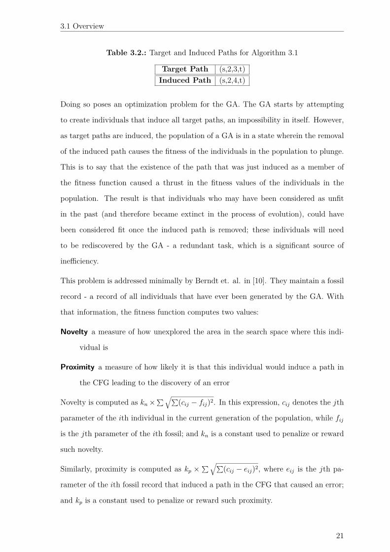
3.1 Overview
di�erence between 4 and the given value is |4 ≠ A| = 1. Similarly, V = 1 since there
is exactly one unmatched node between the induced and target paths. Thus, the IF
for this (target path, induced path) pair is 2.
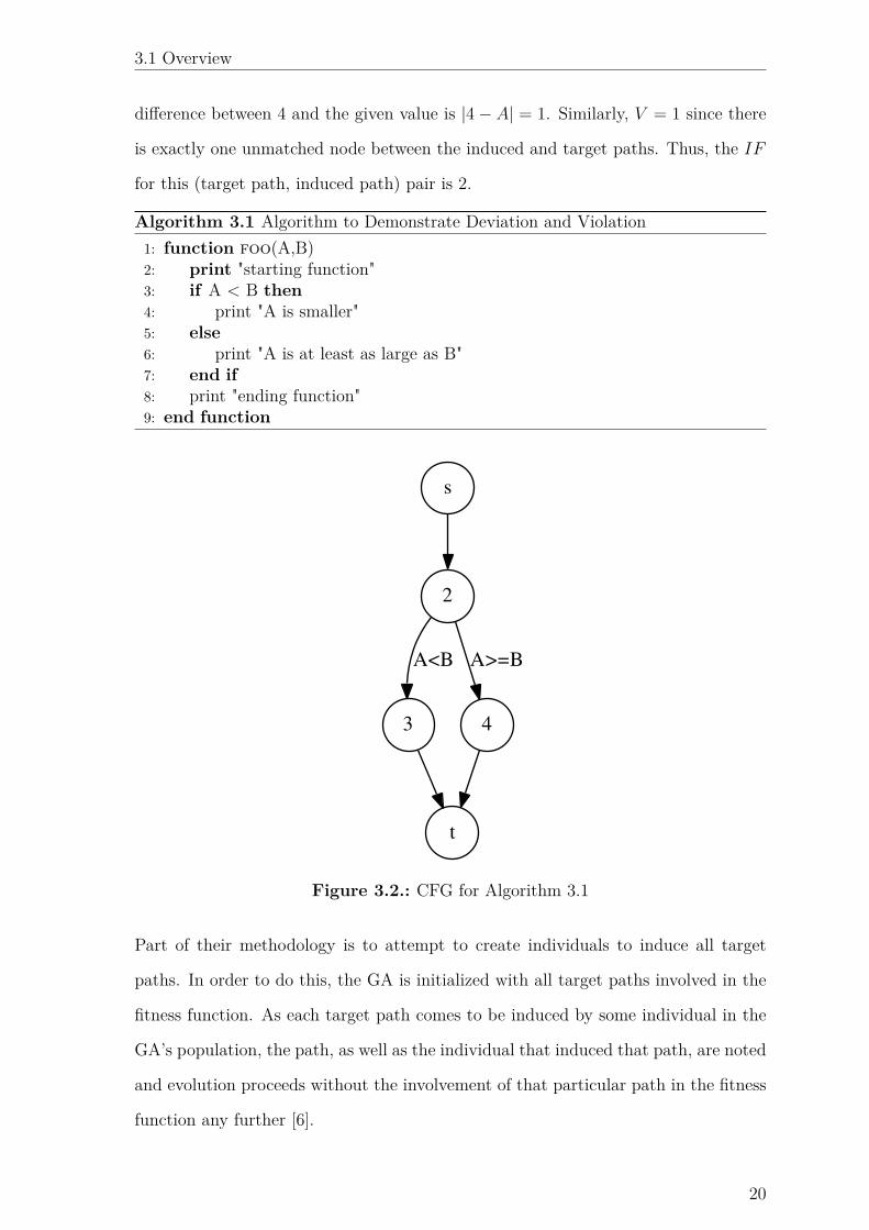
Algorithm 3.1 Algorithm to Demonstrate Deviation and Violation1: function foo(A,B)2: print "starting function"3: if A < B then
4: print "A is smaller"5: else
6: print "A is at least as large as B"7: end if
8: print "ending function"9: end function
s
2
t
3
A<B
4
A>=B
Figure 3.2.: CFG for Algorithm 3.1
Part of their methodology is to attempt to create individuals to induce all target
paths. In order to do this, the GA is initialized with all target paths involved in the
fitness function. As each target path comes to be induced by some individual in the
GA’s population, the path, as well as the individual that induced that path, are noted
and evolution proceeds without the involvement of that particular path in the fitness
function any further [6].
20
3.1 Overview
Table 3.2.: Target and Induced Paths for Algorithm 3.1
Target Path (s,2,3,t)Induced Path (s,2,4,t)
Doing so poses an optimization problem for the GA. The GA starts by attempting
to create individuals that induce all target paths, an impossibility in itself. However,
as target paths are induced, the population of a GA is in a state wherein the removal
of the induced path causes the fitness of the individuals in the population to plunge.
This is to say that the existence of the path that was just induced as a member of
the fitness function caused a thrust in the fitness values of the individuals in the
population. The result is that individuals who may have been considered as unfit
in the past (and therefore became extinct in the process of evolution), could have
been considered fit once the induced path is removed; these individuals will need
to be rediscovered by the GA - a redundant task, which is a significant source of
ine�ciency.
This problem is addressed minimally by Berndt et. al. in [10]. They maintain a fossil
record - a record of all individuals that have ever been generated by the GA. With
that information, the fitness function computes two values:
Novelty a measure of how unexplored the area in the search space where this indi-
vidual is
Proximity a measure of how likely it is that this individual would induce a path in
the CFG leading to the discovery of an error
Novelty is computed as kn
◊ q Òq(cij
≠ fij
)2. In this expression, cij
denotes the jth
parameter of the ith individual in the current generation of the population, while fij
is the jth parameter of the ith fossil; and kn
is a constant used to penalize or reward
such novelty.
Similarly, proximity is computed as kp
◊ q Òq(cij
≠ eij
)2, where eij
is the jth pa-
rameter of the ith fossil record that induced a path in the CFG that caused an error;
and kp
is a constant used to penalize or reward such proximity.
21
3.1 Overview
In order to force the discovery of new inputs, kn
is kept high and kp
is kept low.
It is important to note at this point, that because of the definition of the fitness func-
tion, the computation of the fitness function becomes progressively more expensive
over time. This is because the fitness function has a time complexity of O(F ◊ E),
where F is the size of the fossil record and E is the size of the subset of the fossil
record containing individuals that induced a path in the CFG that caused an error.
Since the fossil record stores each generation cumulatively, F = P ◊G where P is the
population size and G is the number of generations that have passed so far. Thus it
is not di�cult to see that the runtime complexity of the fitness function could easily
surpass O(P 4), which is catastrophically expensive. Further, downplaying the prox-
imity measure may not be a good idea, as there may be a neighborhood of test inputs
in the search space that cause errors, and downplaying proximity would not allow for
thorough exploration of such neighborhoods. However, since Brendt et. al. found
a good balance between kp
and kn
, they are able to force the exploration of exactly
such neighborhoods. Still, such searching is very expensive and possibly dependent
on the SUT.
Further, there is no method proposed to detect whether inputs in a neighborhood
repeatedly induce the same path. This means that although multiple error-causing
inputs may be found, it is possible that all inputs may induce the same path in the
CFG. This results in a run of evolution that appears to be more successful than it
really is. Though this method has been successfully used in [10] to generate inputs
that induce multiple paths in the triangle classification problem, it is still unclear
that it may reliably find such paths in other SUTs.
This problem can be somewhat mitigated by reducing the number of paths that need
to be induced by all test inputs in a run of the GA. Such a reduction in the set
of paths can be accomplished by grouping similar paths together and executing one
run of the GA per group of paths, as outlined in [12]. However, in performing such
grouping, the following conditions need to be met:
1. Only those paths that have adequate subpaths in common with each other
22
3.1 Overview
should be grouped. If this is not the case, the grouping ceases to be meaningful
as it is reduced to a smaller scale version of the work presented in [10].
2. The groups need to be disjoint. If this is not the case, then the fitness function
across some runs of the GA will be redundant, and thus ine�cient.
3. In order for the grouping to a�ord a runtime optimization from a reduction in
the size of the search space, the runs of the GA on each individual group must
be capable of being executed independently of all other runs on other groups.
4. The group sizes should be as even as possible. Suppose this is not the case, and
as a result, one of the groups contains more target paths than the others. Then
a run of the GA with a fitness function using this group would take longer to
finish than a run of the GA with a fitness function using a di�erent group (with
fewer target paths). As a result, even if all GAs were run in parallel, the extra
time required to run a GA with this larger group of target paths will slow down
the time required to complete the run of the overall set of GAs. However, this
will not be the case if all groups contained an equal number of target paths; in
which case, if the overall set of GAs were run in parallel, they would all finish in
approximately equal amounts of time. With this in mind, Dong et. al. divide
P target paths into M groups such that each group contains approximately P
M
paths, and the di�erence in size between any two groups is at most 1.
Dong et. al. suggest that the measure expressed in equation (3.2) should be used to
compute similarity between two target paths; and that the paths can be grouped to-
gether if the similarity is higher than a threshold that they determined experimentally
[12].
s(pi
, pj
) = |pi
fl pj
|max(|p
i
|, |pj
|) (3.2)
where pi
, pj
are target paths
23

3.1 Overview
and |pi
| is the number of nodes in path pi
and |pi
fl pj
| are the number of consecutive identical nodes in paths pi
and pj
.
Note that s(p, p) = 1 for all paths p.
It seems logical that the formation of these groups should be dictated by the similarity
index computed by equation (3.2). However, Dong et. al. choose to partition target
paths among groups by selecting the P
M
most similar remaining target paths. While
this method of partitioning target paths into groups would work for the first few
groups, it is trivial to see that in the worst case, the last group will be composed of
paths that are very dissimilar to each other. As a result, a run of the GA on such a
last group would indeed be a scaled down version of a run of the GA described in [6]
and would su�er from the same evolutionary bottleneck discussed above.
Still, each run of the GA within a group still functions as does the GA presented in
[6]. The only advantage is that the search space is much narrower and the search
is therefore restricted to a smaller neighborhood of the original search space. Fur-
thermore, since the GA starts with a random population initialization as it normally
would, this information about the narrowed search space is lost. Though it is true
that this information would be discovered quite quickly, it is still a learning that is
not strictly necessary for the GA to undergo. A GA might indeed perform better
if the initial population covered the narrow neighborhood of the search space more
thoroughly, than the the entire search space evenly.
Given today’s advances in computational power, focusing more on forming prudent
groups rather equal sized groups might lead to a better evolutionary run-time. For
instance, if in the worst case, a group contains several very dissimilar paths, then it
becomes analogous to running the GA described in [6] for a smaller number of paths.
Hence, a run of the GA on that group might itself be a bottleneck, almost as severe
as executing one run of the GA for all target paths. Thus, it would likely be wiser
to create groups of variable size which contain paths that share a similarity higher
than an experimentally determined threshold. Intuitively, this provides more of a
24

3.1 Overview
guarantee that all machines executing a run of the GA on some input would complete
execution in minimal maximum running time.
This is exactly the notion explored by Gong et. al. in a follow up paper [13] in which
target paths are grouped together only if they have a high similarity8 between them.
Once such groups are formed (note that the number of groups has an upper bound of
the number of paths), a run of the GA is executed for each group. While in this case,
the groups are formed well (to contain only paths that are very similar), the problem
still remains that the initial population is created without using the knowledge that
all the target paths in a group are in a narrow neighborhood of the search space.
The GA is forced to learn this with the imposed penalty in the fitness function that
penalizes individuals for not inducing the required target paths. Still, there are two
problems with this approach:
1. The GA is required to learn that all the target paths (and therefore the fittest
individuals to be evolved) are located in a relatively small neighborhood in the
search space.
2. The fitness function still compares all individuals in a population to all target
paths in a group.
The e�ects of (item 1) are somewhat mitigated by the introduction of the penalty;
but that is still an ad-hoc reactionary solution and does not preempt the problem.
Rather, it foresees the problem, and does nothing to prevent it from happening. A
GA with an initial population that explored this neighborhood more thoroughly is
more likely to produce results in a more e�cient manner
On the other hand, (item 2) is an improvement on past technology. Still, it can be
improved further. Clearly, the most accurate and directed evolution can be designed
for exactly one path. Yet, it does not make sense to make several singleton groups
(for that would negate the purpose of grouping target paths). An improvement over
this will be suggested and discussed in the methodology.
8Similarity is computed as s(pi
, pj
) = k≠1max(|pi|,|pj |) , where p
i
and pj
share the first k nodes
25
3.2 One For All (OFA)
The literature holds examples of other representations of the problem space as well.
For example, Zhang et. al. use a Petri Net representation to generate inputs with
which to test multimedia applications [14]. They use petri nets as an alternative
representation of the SUT (as compared with the CFG representation used in this
thesis). Further, they rely on constraint solvers to facilitate input generation and
only test for reachability. This is loosely related to the notion of detecting infeasible
paths (and thus identifying code bloat) in static white box testing9. While Petri Nets
are a helpful representation tool, they are inappropriate for use in this thesis as they
cause an additional layer of abstraction and transformation between the source code
of the SUT and the input generation mechanism.
Finally, Labiche et. al. use GAs to test real-time systems but are more focussed on
reducing the amount of compute time required by these systems at run-time, so as
not to delay the returning of results, even when under heavy load [15]; or to determine
the order in which software should be tested in order to minimize the amount of time
required for testing bootstrap activities such as method stubbing [16]. These focus
less on generating the inputs with which to test software itself, and are therefore
considered out of the scope of this thesis.
It is clear from the reviewed publications that the current methodologies can be
broadly classified into the following two approaches.
3.2. One For All (OFA)
Under this paradigm, one run of a GA is used to generate test inputs that induce
all target paths. The fitness measure used to compute the fitness of an individual,
under this paradigm, measures a defined distance between the path induced by the
individual (or the inputs that it represents) and each of the target paths. These
distances then become the inputs to the fitness function which applies some form of
normalization to these values.9see sec. 2.5 for more
26
3.2 One For All (OFA)
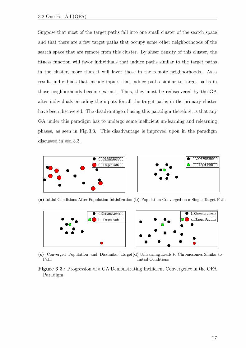
Suppose that most of the target paths fall into one small cluster of the search space
and that there are a few target paths that occupy some other neighborhoods of the
search space that are remote from this cluster. By sheer density of this cluster, the
fitness function will favor individuals that induce paths similar to the target paths
in the cluster, more than it will favor those in the remote neighborhoods. As a
result, individuals that encode inputs that induce paths similar to target paths in
those neighborhoods become extinct. Thus, they must be rediscovered by the GA
after individuals encoding the inputs for all the target paths in the primary cluster
have been discovered. The disadvantage of using this paradigm therefore, is that any
GA under this paradigm has to undergo some ine�cient un-learning and relearning
phases, as seen in Fig. 3.3. This disadvantage is improved upon in the paradigm
discussed in sec. 3.3.
(a) Initial Conditions After Population Initialization (b) Population Converged on a Single Target Path
(c) Converged Population and Dissimilar TargetPath
(d) Unlearning Leads to Chromosomes Similar toInitial Conditions
Figure 3.3.: Progression of a GA Demonstrating Ine�cient Convergence in the OFAParadigm
27
3.3 One For Each (OFE)
3.3. One For Each (OFE)
Under this paradigm, one run of a GA is tasked with discovering an individual that
encodes the inputs for a specific target path. However, if there exists a cluster of
very similar target paths, then each run of a GA, tasked with discovering one of those
target paths, will have to independently converge on that cluster in the search space.
This implies multiple instances of independent and redundant learning on the part
of several GAs. This redundant learning is ine�cient and is improved upon by the
paradigm discussed in sec. 3.2.
3.4. Summary
Both the OFA and the OFE methods combat each other’s shortcomings without
addressing their own. Clearly, a hybrid solution encompassing both their strengths
would be beneficial. Such a hybrid would also mitigate the problems that GAs face,
given the uncertain nature of the randomness of their initialization conditions.
28
4. Implementation
4.1. Overview
As discussed in chapter 3, there are several problems concerning the use of one run
of a GA per collection of target paths in order to discover test input data for a SUT.
At the same time, executing one run of the GA per target path seems ine�cient.
Therefore, a balance needs to be struck with a hybrid system. This thesis proposes
to develop such a more appropriate hybrid method to use GAs and ESs to discover
test input data for a SUT.
Consider the merge sort algorithm. It functions by recursively splitting a list of
numbers in half, sorting each half and merging corresponding halves together [17].
The first version of the algorithm, indeed the one still taught in introductory computer
science courses today, uses a linear insertion technique to merge corresponding halves
of lists; i.e. to merge two lists containing n elements each, a total of n comparisons
are made. Of importance is the notion that the input list is first recursively divided
into sublists until at least one and at most two singleton lists remain.
With a little analysis, it is not di�cult to see that merging techniques other than
linear insertion may be used to merge two sorted halves of lists, as explored in [17].
Further, note that this is only one implementation to recursively use merge sort on
each half of the divided list. Indeed it is a logical choice in the interest of runtime
e�ciency, though it is also possible to use any other sorting technique to sort the
sublists and any merging technique to merge sorted sublists.
29
4.1 Overview
With that in mind, this thesis explores a hybrid evolutionary strategy and genetic
algorithm to discover test input data for a SUT. Many works in the literature have
been reviewed that use a GA to either discover one target path 1, several target paths
iteratively2, or several target paths iteratively within a grouped set of similar target
paths (without giving the GA any knowledge about such a similarity)3.
In the spirit of the work presented in [13], this thesis will generate groupings (i.e.
bins) of similar target paths. However, a run of the GA for each group will not start
with a normal random population generation function. Rather, the initial population
will be primed in some sense to reflect the context of the grouping of similar target
paths. Thus, the algorithm begins with an ES with a random initial population,
recursively classifying target paths into bins of similar target paths. This is done
by computing a similarity index between every pair of target paths4 and assigning
multiple target paths to a specific bin only if their mutual similarity indices surpass
an experimentally determined threshold. At each level of the recursion, an individual
from the current population is computed to be the seed (explained in sec. 4.5) for
each bin and mutated several times to spawn the next generation of the population
of individuals for that particular bin. This continues until there is only one target
path left in a bin; at which point, the GA is used with the spawned population, to
find the test inputs that induce the only target path in the bin.
All algorithms presented in this thesis were implemented using the Python program-
ming language, with the trace and Pyvolution
5 packages, and their dependencies
with Python version 2.7.3.
1see chapter 3 for more2see chapter 3 for more3see chapter 3 for more4see Algorithm 4.55See sec. 4.7
30
4.2 Workflow
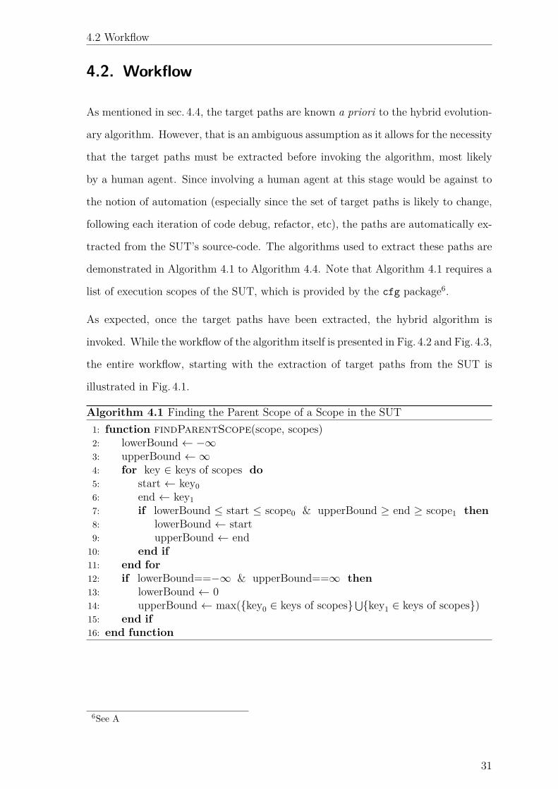
4.2. Workflow
As mentioned in sec. 4.4, the target paths are known a priori to the hybrid evolution-
ary algorithm. However, that is an ambiguous assumption as it allows for the necessity
that the target paths must be extracted before invoking the algorithm, most likely
by a human agent. Since involving a human agent at this stage would be against to
the notion of automation (especially since the set of target paths is likely to change,
following each iteration of code debug, refactor, etc), the paths are automatically ex-
tracted from the SUT’s source-code. The algorithms used to extract these paths are
demonstrated in Algorithm 4.1 to Algorithm 4.4. Note that Algorithm 4.1 requires a
list of execution scopes of the SUT, which is provided by the cfg package6.
As expected, once the target paths have been extracted, the hybrid algorithm is
invoked. While the workflow of the algorithm itself is presented in Fig. 4.2 and Fig. 4.3,
the entire workflow, starting with the extraction of target paths from the SUT is
illustrated in Fig. 4.1.
Algorithm 4.1 Finding the Parent Scope of a Scope in the SUT1: function findParentScope(scope, scopes)2: lowerBound Ω ≠Œ3: upperBound Ω Œ4: for key œ keys of scopes do
5: start Ω key06: end Ω key17: if lowerBound Æ start Æ scope0 & upperBound Ø end Ø scope1 then
8: lowerBound Ω start9: upperBound Ω end
10: end if
11: end for
12: if lowerBound==≠Œ & upperBound==Œ then
13: lowerBound Ω 014: upperBound Ω max({key0 œ keys of scopes} t{key1 œ keys of scopes})15: end if
16: end function
6See A
31
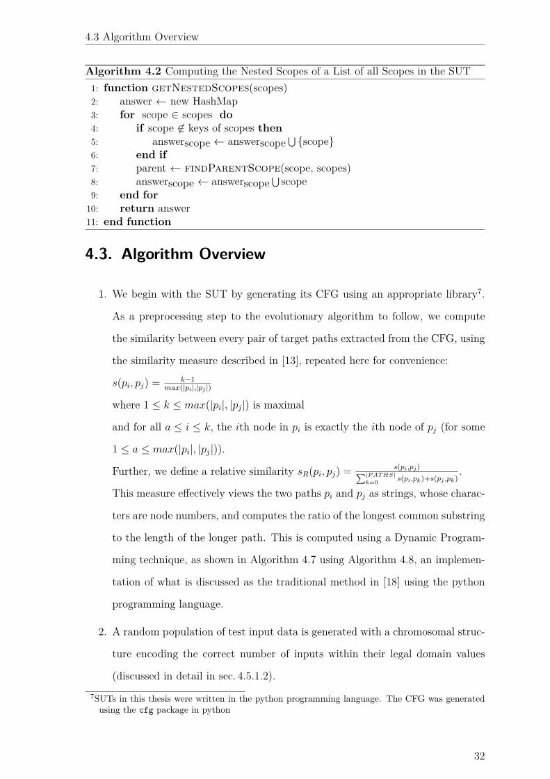
4.3 Algorithm Overview
Algorithm 4.2 Computing the Nested Scopes of a List of all Scopes in the SUT1: function getNestedScopes(scopes)2: answer Ω new HashMap3: for scope œ scopes do
4: if scope ”œ keys of scopes then
5: answerscope Ω answerscopet {scope}
6: end if
7: parent Ω findParentScope(scope, scopes)8: answerscope Ω answerscope
t scope9: end for
10: return answer11: end function
4.3. Algorithm Overview
1. We begin with the SUT by generating its CFG using an appropriate library7.
As a preprocessing step to the evolutionary algorithm to follow, we compute
the similarity between every pair of target paths extracted from the CFG, using
the similarity measure described in [13], repeated here for convenience:
s(pi
, pj
) = k≠1max(|pi|,|pj |)
where 1 Æ k Æ max(|pi
|, |pj
|) is maximal
and for all a Æ i Æ k, the ith node in pi
is exactly the ith node of pj
(for some
1 Æ a Æ max(|pi
|, |pj
|)).
Further, we define a relative similarity sR
(pi
, pj
) = s(pi,pj)q|P AT HS|k=0 s(pi,pk)+s(pj ,pk)
.
This measure e�ectively views the two paths pi
and pj
as strings, whose charac-
ters are node numbers, and computes the ratio of the longest common substring
to the length of the longer path. This is computed using a Dynamic Program-
ming technique, as shown in Algorithm 4.7 using Algorithm 4.8, an implemen-
tation of what is discussed as the traditional method in [18] using the python
programming language.
2. A random population of test input data is generated with a chromosomal struc-
ture encoding the correct number of inputs within their legal domain values
(discussed in detail in sec. 4.5.1.2).7SUTs in this thesis were written in the python programming language. The CFG was generated
using the cfg package in python
32

4.3 Algorithm Overview
3. The target paths are divided into bins based on target paths whose similarity is
greater than an experimentally determined threshold. This binning algorithm is
shown in Algorithm 4.5 which, in turn, uses Algorithm 4.6, Algorithm 4.7 and
Algorithm 4.8.
4. The chromosome in the population that has the highest fitness among each
group is then considered to be the seed for the next generation of test input
data for that group of target paths. The algorithm used to determine the seed
for each group is shown in Algorithm 4.9.
5. This chromosome is mutated several times in various ways to form the new
population for the group of similar target paths.
6. Repeat steps item 3 - item 5 until the resulting groups of similar target paths
are all singletons.
7. Execute a run of the GA algorithm per target path (i.e. per singleton group of
target paths) until a test input is discovered that induces the target path.
8. Record the discovered test input and the target path and terminate the evolu-
tionary process for that group.
This algorithm is visualized in Figure Fig. 4.2 on page 51 and Figure Fig. 4.3 on page
52.
Despite the drawbacks to executing separate runs of the evolutionary process per
group or target path, the following justifications can be made:
1. This method is highly parallelizable.
2. Due to the small size of each group, the evolutionary process to execute a run
of the GA would not take as long.
3. Since the initial population for the GA has already undergone several genera-
tions of evolution, the initial population is already composed of multiple very
33
4.4 Binning, Seed Finding and Similarity Computation Algorithms
fit chromosomes8. This would only expedite the process of evolution.
4. Since the GAs themselves can be executed fairly quickly (as explained above),
the maximum delay of the last machine to finish such a run of the GA in a
parallel environment can be reduced.
4.4. Binning, Seed Finding and Similarity
Computation Algorithms
Since the target paths are known before starting the hybrid evolutionary algorithm,
the core algorithm classifies the target paths into bins, finds a seed per bin and spawns
a new population of individuals per bin, by mutating the seed. The algorithm then
recursively repeats this process until only one target path remains in any bin; at which
time, a GA is used on the bin(s) containing only one target path, while the recursion
continues on all other bins. This process is illustrated in Fig. 4.4 (in the interest of
brevity, the process flow of only one bin is expanded). The algorithms associated with
this process flow are described in this section.
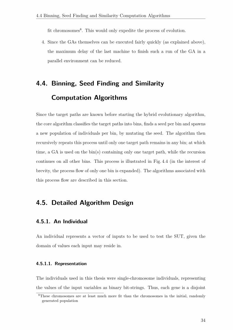
4.5. Detailed Algorithm Design
4.5.1. An Individual
An individual represents a vector of inputs to be used to test the SUT, given the
domain of values each input may reside in.
4.5.1.1. Representation
The individuals used in this thesis were single-chromosome individuals, representing
the values of the input variables as binary bit-strings. Thus, each gene is a disjoint8These chromosomes are at least much more fit than the chromosomes in the initial, randomly
generated population
34

4.5 Detailed Algorithm Design
section of the chromosome that encodes the value for a particular input variable. For
example, Fig. C.1 (repeated in sec. 4.5.1.2 for convenience) illustrates the structure of
a chromosome encoding the three inputs that form the input vector <3,4,5>.
4.5.1.2. Creation
In this example, each gene is created by concatenating the results of four calls to a
random number generator to generate a number in the appropriate domain9. This
number is then converted into a binary bit-string representation using a function call
provided in the Python standard library. Once converted, this binary bit string is
padded with 0s on the left to ensure that it is represented by a full four bits. This
algorithm is visualized in Fig. 4.6.
Input 1 Input 2 Input 3
0 1 1 1 0 0 1 0 1
Figure 4.5.: Example Chromosome for Input Vector <3,4,5>
4.5.2. Population Initialization
4.5.2.1. Initialization for the Hybrid Algorithm
Given
1. the number of input variables (N)
2. the data types and the ranges of domain for the input variables
3. the number of individuals in the population (popSize)
the initial population is created by creating popSize many unique individuals. The
creation of each individual is visualized in Fig. 4.6, while the generation of the initial
population is visualized in Fig. 4.7.
9Part of Python’s standard library
35
4.5 Detailed Algorithm Design
4.5.2.2. Initialization in the Seeded Evolutionary Strategy and the Seeded
Genetic Algorithm
After the target paths have been binned (by the binning algorithm described in
sec. 4.4), a seed individual is computed for each bin. This done by Algorithm 4.9
by computing the relative similarities between the path induced by each individual
and the bin or target paths. The individual that induces the path with the highest
relative similarity is considered to be the seed for that bin
4.5.3. Computing the Fitness of an Individual
The fitness of an individual is computed against a target path.
First, the chromosome of the individual is decoded into the test input values. The
SUT is then run on these variables, using a software harness10 and the path of ex-
ecution (the induced path) is tracedfootnote 10. Next, the similarity between the
induced path and the target path is computed (as discussed in sec. 4.3. This com-
puted similarity is the fitness of the individual. This process is visualized in Fig. 4.8.
4.5.4. Selecting Individuals for Mating
Individuals in the population are selected in a fitness-proportional manner by using
a roulette-wheel selection scheme as described in sec. C.1.7.
4.5.5. Crossover
A one-point crossover mechanism was used to perform crossover operations between
pairs of individuals. This was used over a uniform crossover scheme, as is it possible
that changing one input variable to a SUT may significantly alter the induced path.
A one-point crossover ensures that only one variable’s value is changed. On the other
hand, the likelihood of only one input parameter to the SUT changing as the result10This is accomplished by using the tracer module in Python’s standard library
36
4.6 Implementation Parameters
of a a uniform crossover is very low. It is for similar reasons that n-point crossovers
were also not considered (for n > 1).
4.5.6. Mutation
A point mutation (as discussed in sec. C.1.10) was implemented. This mutation mech-
anism flips one random bit in the encoding of one of the input variables.
4.5.7. Spawning
A spawning function is used in the seeded GA and seeded ES algorithms to produce
a full population of individuals from a seed. The spawn function used was exactly
the mutation function. This allows the algorithm to generate a full population of
individuals that are very similar to the seed. This allows for the creation of a pop-
ulation that is highly localized to the neighborhood in the search space occupied by
the target paths in the bin. This process is visualized in Fig. 4.4.
4.5.8. Termination
The Seeded GA algorithm terminates either when an individual that encodes inputs
that induce the desired target path is found; or when the maximum number of allowed
fitness evaluations has been reached.
4.6. Implementation Parameters
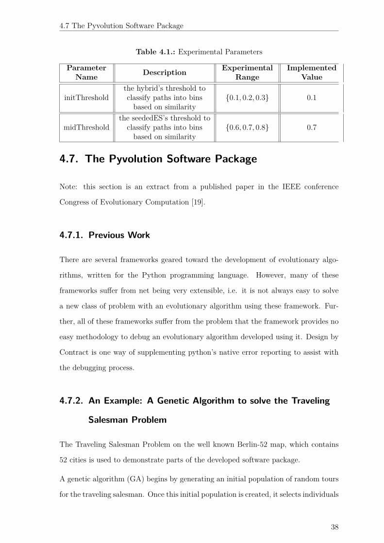
The implemented algorithmic parameters for each SUT are listed in Tab. 4.1. The
e�ects of these values are discussed in chapter 5.
37
4.7 The Pyvolution Software Package
Table 4.1.: Experimental Parameters
Parameter
Name
Description
Experimental
Range
Implemented
Value
initThresholdthe hybrid’s threshold toclassify paths into bins
based on similarity{0.1, 0.2, 0.3} 0.1
midThresholdthe seededES’s threshold to
classify paths into binsbased on similarity
{0.6, 0.7, 0.8} 0.7
4.7. The Pyvolution Software Package
Note: this section is an extract from a published paper in the IEEE conference
Congress of Evolutionary Computation [19].
4.7.1. Previous Work
There are several frameworks geared toward the development of evolutionary algo-
rithms, written for the Python programming language. However, many of these
frameworks su�er from net being very extensible, i.e. it is not always easy to solve
a new class of problem with an evolutionary algorithm using these framework. Fur-
ther, all of these frameworks su�er from the problem that the framework provides no
easy methodology to debug an evolutionary algorithm developed using it. Design by
Contract is one way of supplementing python’s native error reporting to assist with
the debugging process.
4.7.2. An Example: A Genetic Algorithm to solve the Traveling
Salesman Problem
The Traveling Salesman Problem on the well known Berlin-52 map, which contains
52 cities is used to demonstrate parts of the developed software package.
A genetic algorithm (GA) begins by generating an initial population of random tours
for the traveling salesman. Once this initial population is created, it selects individuals
38
4.7 The Pyvolution Software Package
to probabilistically crossover and mutate, thereby making child individuals, which
comprise the next generation of this population. Repeating this process of selection,
crossover and mutation over several generations allows the GA to converge on an
optimal solution.
An Individual Individuals in a GA to solve this problem are made up of one chro-
mosome. This chromosome is a list of 52 integers, each one representing a city on
the map. In order for an individual to represent a legal solution in the solution space,
the chromosome is a permutation of {0, 1, 2, ..., 51}, thus making it a valid tour for
the traveling salesman problem.
Fitness of an Individual Since the optimal solution for this problem is an individual
whose tour length is minimal, the fitness of each individual could be the length of the
tour it represents. However, since the goal is to maximize the fitness, a better fitness
measure of an individual would be the negative of the length of the tour it represents.
This can be easily computed under the following assumptions:
1. Each of the 52 cities on the map is represented as a point on the xy plane
2. There is a straight line (road) connecting every pair of the 52 cities on the map
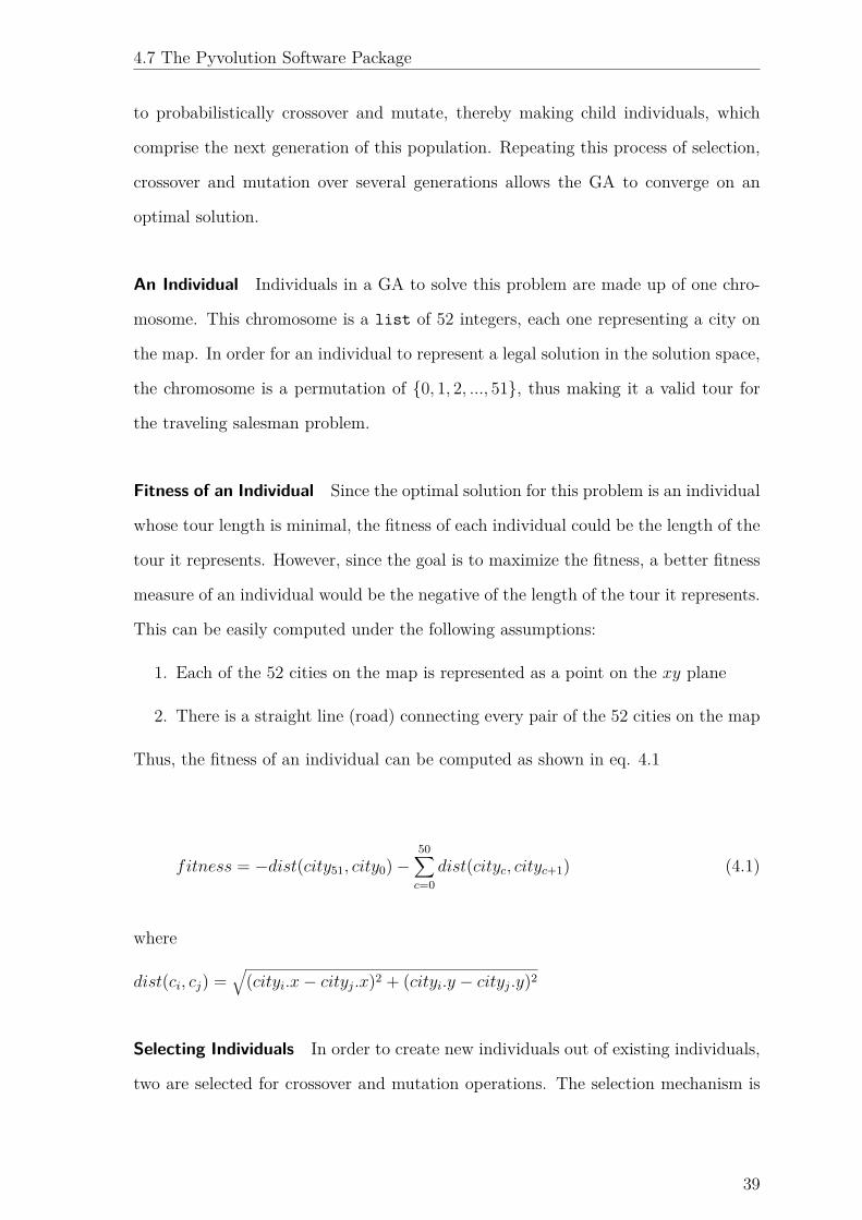
Thus, the fitness of an individual can be computed as shown in eq. 4.1
fitness = ≠dist(city51, city0) ≠50ÿ
c=0dist(city
c
, cityc+1) (4.1)
where
dist(ci
, cj
) =Ò
(cityi
.x ≠ cityj
.x)2 + (cityi
.y ≠ cityj
.y)2
Selecting Individuals In order to create new individuals out of existing individuals,
two are selected for crossover and mutation operations. The selection mechanism is
39

4.7 The Pyvolution Software Package
fitness proportional, meaning that individuals with higher fitness are selected more
often than individuals with lower fitness.
Crossover A crossover is an operation that takes two parent individuals and creates
a new child individual, whose chromosomes are comprised of parts of the correspond-
ing chromosomes from both parents (as explained in sec. C.1.9). In the case of this
traveling salesman problem, one possible crossover function is defined as follows:
1. Select points A and B such that 0 < A < B < 51
2. Make an empty child chromosome which is intended to hold 52 cities (a new
tour for the traveling salesman)
3. Copy over all the cities between points A and B in the tour represented by
parent1 into the child chromosome
4. Copy over all the cities before point A and after point B in the tour represented
by parent2 into the corresponding location in the child chromosome, as long as
the city does not already exist between points A and B in the child chromosome.
5. Fill in the remaining cities in the child chromosome based on the order in which
they appear in parent1.
6. Insert this child chromosome into a new individual - the child individual of the
crossover.
Note that it is imperative that the child individual of a crossover represent a legal
solution so as to ensure that the GA does not create individuals that are outside the
solution space.
Mutation As explained in sec. C.1.10, a mutation is an operation that slightly
changes an individual. One possible mutation is to swap the positions of two cities
in the tour. Another possible mutation is to reverse the order of the cities in one
contiguous part of the tour.
40

4.7 The Pyvolution Software Package
Note that it is imperative that a mutated individual must still represent a legal
solution so as to ensure that the GA does not create individuals that are outside the
solution space.
4.7.3. Introducing Design by Contract
The Design by Contract Principle Design by contract (DbC) is the principle that
interfaces between modules of a software system should be governed by precise speci-
fications. The contracts will cover mutual obligations (preconditions), benefits (post-
conditions), and consistency constraints (invariants) [20]. This principle is especially
applicable in large modular systems with multiple levels of abstraction, such as a
framework for implementing GAs.
The Advantage of Using DbC in this Framework Two of the core design principles
of the python programming language are
1. Almost all expressions that a programmer tries to compute must be computed
in some meaningful way.
2. All error reporting and tracebacks should be meaningful in order to help a
programmer better debug their program. In particular, core-dumps and crashes
should be avoided.
In most cases, these are very desirable principles in a programming language. How-
ever, when working with Genetic Algorithms (GAs), where even simple o�-by-one
errors can cause individual solutions in a population to leave the solution space and
where mutation and crossover operations are probabilistic, bugs become di�cult to
reproduce and traditional step-through debugging becomes infeasible (except in a
small subset of the program’s functional body). While this error reporting explains
why the GA may crash, it does very little to reveal the real source of the error (for
example, it may be clear that two variables of very di�erent data types may not
be added together, but the bug that causes either variable to be of that di�erent
41
4.7 The Pyvolution Software Package
datatype is not identified). Thus, whereas the error messages may be well written for
most other algorithms, they are rendered far too cryptic to help debug a GA.
Further, due to the amount of data that a GA works with on the stack, traditional
print-debugging (or logging) would also be infeasible as the signal-to-noise ratio in
the debug logs would be too low to be useful to a programmer.
One particularly di�cult bug was found to be caused by mistyping if a>b: a,b =
b,a as if a<b: a,b = b,a in the crossover function for the GA solving the trav-
eling salesman problem [21]. This had the e�ect of causing this error, mid evolution:
IndexError: pop from empty list. This is because the correctly implemented
crossover function, despite implementing its specification accurately, made certain
assumptions that were incorrect. These assumptions were incorrect due to the afore-
mentioned mistyping. However, the raised IndexError does not provide any infor-
mation as to the source of this error.
Further, assuming that the GA runs without any errors, if the end result of a run
of the GA is unfavorable or unexpected, it is unclear as to whether this divergence
in expectations was caused by the stochastic nature of evolution (and incorrectly
programmed parameters thereof) or by faulty programming logic. As a result, im-
plementing contracts for each of the functions in this framework allows programmers
to catch errors in programming logic early, trace the error to the buggy function
in the program, and eliminate programming errors as the reason for unexpected re-
sults at the end of a run of the GA (assuming that the correct contracts have been
implemented).
4.7.4. A DbC Framework for Python
In order to implement DbC to this GA framework, two packages were evaluated.
These packages are reviewed in this section
42
4.7 The Pyvolution Software Package
PyContract PyContract is a DbC package that allows a programmer to annotate
functions with contract expressions. The fact that its syntax allows for the devel-
opment of richer contract expressions makes up for the shortcomings of other DbC
frameworks, making it the preferred framework with which to implement DbC ex-
pressions for this package.
For example, the contract expressions in algorithm Algorithm 4.10 for a function that
multiplies two matrices denotes that:
1. The input parameter a is a nested list of positive row and column dimensions.
2. The input parameter b is an array of positive row and column dimensions.
3. The number of rows in b is equal to the number of columns in a.
a) This ensures that a and b are of compatible dimensionalities.
4. The function returns an array of M rows and P columns.
5. The inputs are unchanged
In addition, PyContract also allows for the expression of class invariants. These are
expressible with the inv declaration in the contract expressions along with referencing
self. However, there is a limitation to PyContract’s ability to express invariants in
functions. For example, it is not possible to express contracts about loop invariants
whose expressions contain variables that are not class variables, but are instead local
to the scope of the function itself. In order to express such invariants in this GA
framework, a hybrid approach using both PyContract and assert statements native
to Python were used.
As previously stated, the DbC implementation for this GA framework is a hybrid
of PyContract and assert statements native to the python programming language.
For example, the crossover function described in section sec. 4.7.2 has the contracts
shown in algorithm Algorithm 4.11 (explained in table 4.7.4).
43
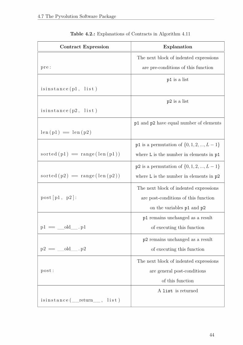
4.7 The Pyvolution Software Package
Table 4.2.: Explanations of Contracts in Algorithm 4.11
Contract Expression Explanation
pre :
The next block of indented expressions
are pre-conditions of this function
i s i n s t a n c e (p1 , l i s t )
p1 is a list
i s i n s t a n c e (p2 , l i s t )
p2 is a list
l en ( p1 ) == len ( p2 )
p1 and p2 have equal number of elements
so r t ed ( p1 ) == range ( l en ( p1 ) )
p1 is a permutation of {0, 1, 2, ..., L ≠ 1}
where L is the number in elements in p1
so r t ed ( p2 ) == range ( l en ( p2 ) )
p2 is a permutation of {0, 1, 2, ..., L ≠ 1}
where L is the number in elements in p2
post [ p1 , p2 ] :
The next block of indented expressions
are post-conditions of this function
on the variables p1 and p2
p1 == __old__ . p1
p1 remains unchanged as a result
of executing this function
p2 == __old__ . p2
p2 remains unchanged as a result
of executing this function
post :
The next block of indented expressions
are general post-conditions
of this function
i s i n s t a n c e (__return__ , l i s t )
A list is returned
44
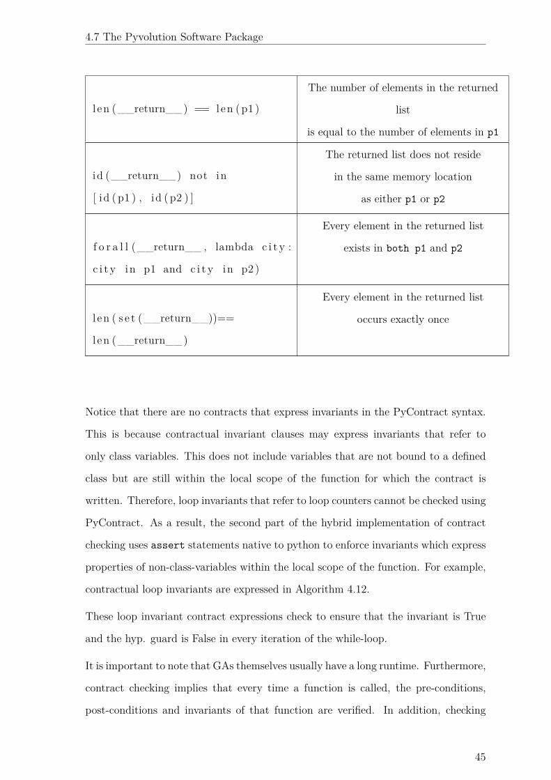
4.7 The Pyvolution Software Package
l en (__return__) == len ( p1 )
The number of elements in the returned
list
is equal to the number of elements in p1
id (__return__) not in
[ id ( p1 ) , id ( p2 ) ]
The returned list does not reside
in the same memory location
as either p1 or p2
f o r a l l (__return__ , lambda c i t y :
c i t y in p1 and c i t y in p2 )
Every element in the returned list
exists in both p1 and p2
l en ( s e t (__return__))==
len (__return__)
Every element in the returned list
occurs exactly once
Notice that there are no contracts that express invariants in the PyContract syntax.
This is because contractual invariant clauses may express invariants that refer to
only class variables. This does not include variables that are not bound to a defined
class but are still within the local scope of the function for which the contract is
written. Therefore, loop invariants that refer to loop counters cannot be checked using
PyContract. As a result, the second part of the hybrid implementation of contract
checking uses assert statements native to python to enforce invariants which express
properties of non-class-variables within the local scope of the function. For example,
contractual loop invariants are expressed in Algorithm 4.12.
These loop invariant contract expressions check to ensure that the invariant is True
and the hyp. guard is False in every iteration of the while-loop.
It is important to note that GAs themselves usually have a long runtime. Furthermore,
contract checking implies that every time a function is called, the pre-conditions,
post-conditions and invariants of that function are verified. In addition, checking
45
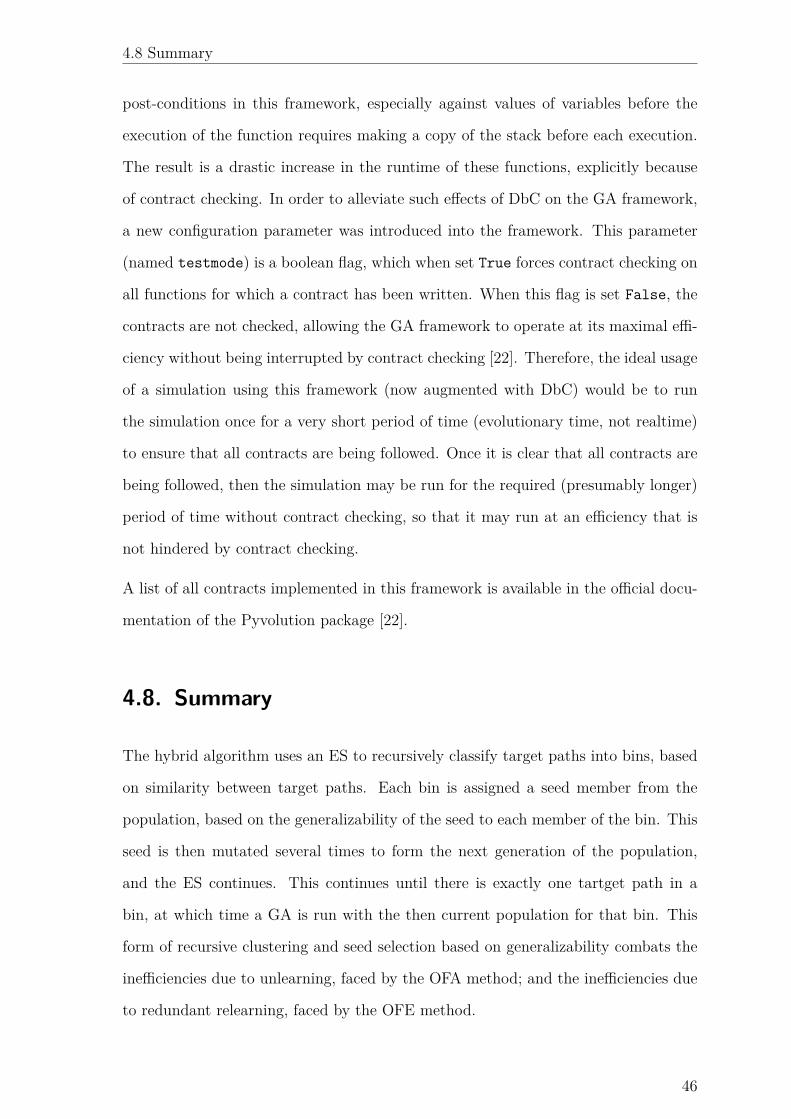
4.8 Summary
post-conditions in this framework, especially against values of variables before the
execution of the function requires making a copy of the stack before each execution.
The result is a drastic increase in the runtime of these functions, explicitly because
of contract checking. In order to alleviate such e�ects of DbC on the GA framework,
a new configuration parameter was introduced into the framework. This parameter
(named testmode) is a boolean flag, which when set True forces contract checking on
all functions for which a contract has been written. When this flag is set False, the
contracts are not checked, allowing the GA framework to operate at its maximal e�-
ciency without being interrupted by contract checking [22]. Therefore, the ideal usage
of a simulation using this framework (now augmented with DbC) would be to run
the simulation once for a very short period of time (evolutionary time, not realtime)
to ensure that all contracts are being followed. Once it is clear that all contracts are
being followed, then the simulation may be run for the required (presumably longer)
period of time without contract checking, so that it may run at an e�ciency that is
not hindered by contract checking.
A list of all contracts implemented in this framework is available in the o�cial docu-
mentation of the Pyvolution package [22].
4.8. Summary
The hybrid algorithm uses an ES to recursively classify target paths into bins, based
on similarity between target paths. Each bin is assigned a seed member from the
population, based on the generalizability of the seed to each member of the bin. This
seed is then mutated several times to form the next generation of the population,
and the ES continues. This continues until there is exactly one tartget path in a
bin, at which time a GA is run with the then current population for that bin. This
form of recursive clustering and seed selection based on generalizability combats the
ine�ciencies due to unlearning, faced by the OFA method; and the ine�ciencies due
to redundant relearning, faced by the OFE method.
46

4.8 Summary
This hybrid evolutionary algorithm is implemented using the Pyvolution evolutionary
algorithms framework; the CFG of the SUT is obtained using the CFG software
package.
47
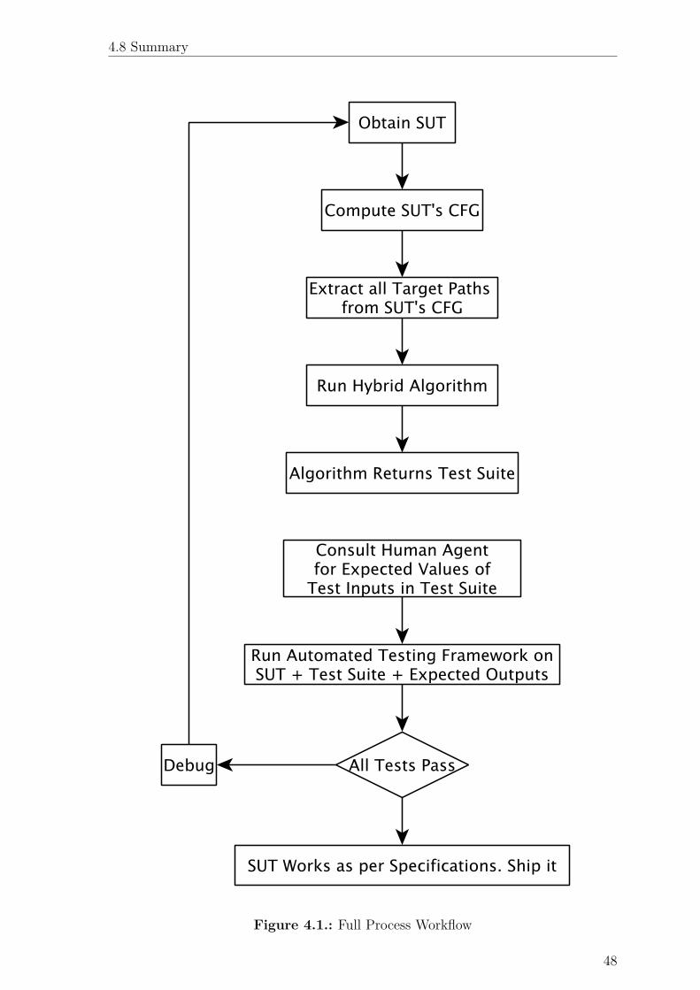
4.8 Summary
Figure 4.1.: Full Process Workflow
48
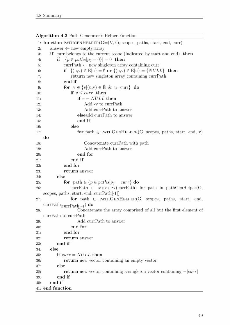
4.8 Summary
Algorithm 4.3 Path Generator’s Helper Function1: function pathgenHelper(G=(V,E), scopes, paths, start, end, curr)2: answer Ω new empty array3: if curr belongs to the current scope (indicated by start and end) then
4: if |{p œ paths|p0 = 0}| = 0 then
5: currPath Ω new singleton array containing curr6: if {(u,v) œ E|u} = ÿ or {(u,v) œ E|u} = {NULL} then
7: return new singleton array containing currPath8: end if
9: for v œ {v|(u,v) œ E & u=curr} do
10: if v Æ curr then
11: if v = NULL then
12: Add -v to currPath13: Add currPath to answer14: elseadd currPath to answer15: end if
16: else
17: for path œ pathGenHelper(G, scopes, paths, start, end, v)do
18: Concatenate currPath with path19: Add currPath to answer20: end for
21: end if
22: end for
23: return answer24: else
25: for path œ {p œ paths|p0 = curr} do
26: currPath Ω memcpy(currPath) for path in pathGenHelper(G,scopes, paths, start, end, currPath[-1])
27: for path œ pathGenHelper(G, scopes, paths, start, end,currPath|currPath|≠1) do
28: Concatenate the array comprised of all but the first element ofcurrPath to currPath
29: Add currPath to answer30: end for
31: end for
32: return answer33: end if
34: else
35: if curr = NULL then
36: return new vector containing an empty vector37: else
38: return new vector containing a singleton vector containing ≠|curr|39: end if
40: end if
41: end function
49
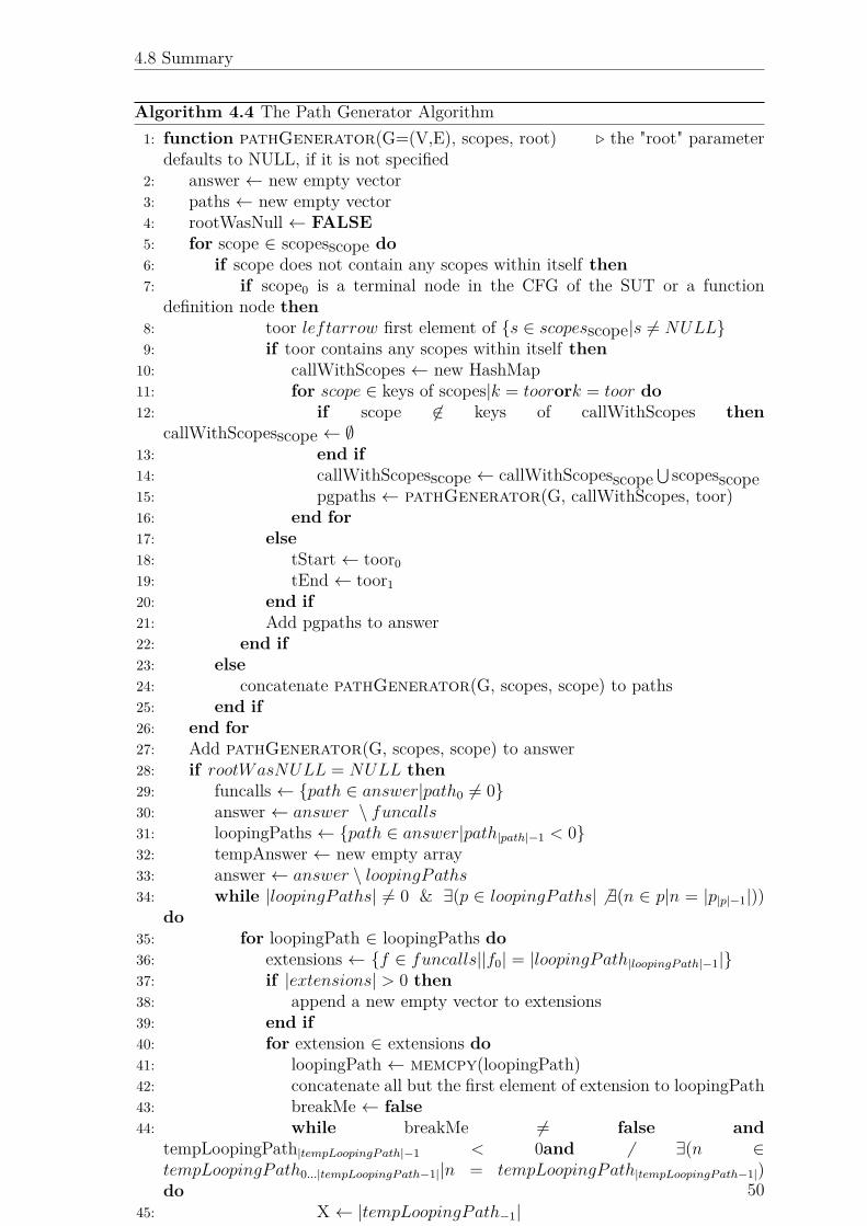
4.8 Summary
Algorithm 4.4 The Path Generator Algorithm1: function pathGenerator(G=(V,E), scopes, root) Û the "root" parameter
defaults to NULL, if it is not specified2: answer Ω new empty vector3: paths Ω new empty vector4: rootWasNull Ω FALSE
5: for scope œ scopesscope do
6: if scope does not contain any scopes within itself then
7: if scope0 is a terminal node in the CFG of the SUT or a functiondefinition node then
8: toor leftarrow first element of {s œ scopesscope|s ”= NULL}9: if toor contains any scopes within itself then
10: callWithScopes Ω new HashMap11: for scope œ keys of scopes|k = toorork = toor do
12: if scope ”œ keys of callWithScopes then
callWithScopesscope Ω ÿ13: end if
14: callWithScopesscope Ω callWithScopesscopet scopesscope
15: pgpaths Ω pathGenerator(G, callWithScopes, toor)16: end for
17: else
18: tStart Ω toor019: tEnd Ω toor120: end if
21: Add pgpaths to answer22: end if
23: else
24: concatenate pathGenerator(G, scopes, scope) to paths25: end if
26: end for
27: Add pathGenerator(G, scopes, scope) to answer28: if rootWasNULL = NULL then
29: funcalls Ω {path œ answer|path0 ”= 0}30: answer Ω answer \ funcalls31: loopingPaths Ω {path œ answer|path|path|≠1 < 0}32: tempAnswer Ω new empty array33: answer Ω answer \ loopingPaths34: while |loopingPaths| ”= 0 & ÷(p œ loopingPaths| ” ÷(n œ p|n = |p|p|≠1|))
do
35: for loopingPath œ loopingPaths do
36: extensions Ω {f œ funcalls||f0| = |loopingPath|loopingP ath|≠1|}37: if |extensions| > 0 then
38: append a new empty vector to extensions39: end if
40: for extension œ extensions do
41: loopingPath Ω memcpy(loopingPath)42: concatenate all but the first element of extension to loopingPath43: breakMe Ω false
44: while breakMe ”= false and
tempLoopingPath|tempLoopingP ath|≠1 < 0and ” ÷(n œtempLoopingPath0...|tempLoopingP ath≠1||n = tempLoopingPath|tempLoopingP ath≠1|)do
45: X Ω |tempLoopingPath≠1|46: Y Ω |the element preceding the second last negative number in tempLoopingPath|47: if X.Y contains outgoing edges in G then
48: toor0 Ω |the element in tempLoopingPath following Y |49: toor1 Ω toor050: Replace the last element in tempLoopingPaths with its
absolute value51: Replace the second last negative element in tempLoop-
ingPaths with its absolute value52: toorParent Ω then immediately enclosing scope of toor53: if ÷(v œ V |toor0 < v < toor0 + 1) then
54: toor Ω a subscope of toor55: callWithScopes Ω all mappings for parent and child
scopes where toor is the parent or one of the children56: for pgh œ pathgenhenper(G, callWithScopes,
paths, toor0, toor1, the next outgoing node from X.Y) do
57: add to answer, the concatenation of all but the lastlast element of tempLoopingPath and pgh
58: end for
59: else
60: for pgh œ pathgenhenper(G, scopes, paths, toor0,toor1, the next outgoing node from X.Y) do
61: add to answer, the concatenation of all but the lastlast element of tempLoopingPath and pgh
62: end for
63: end if
64: break
65: else
66: extensions Ω {f œ funcalls||funcall0| =|tempLoopingPath|tempLoopingP ath|≠1|}
67: for extension œ extensions do
68: Add to answer, the concatenation of all but the lastelement of extension to tempLoopingpath
69: end for
70: break
71: try
72: temp Ω an array of all but the first element of the nextextension in extensions
73: concatenate temp to tempLoopingPath74: catch IndexError
75: do nothing76: end try
77: end if
78: end while
79: end for
80: end for
81: for loopingPath œ answer do last Ω the last element of tempLooping-Path
82: if last œ an array containing all but the last element of tempLoop-ingPath then
83: Set all elements (except for the last one) in tempLoopingPathsto their absolute values
84: end if
85: end for
86: loopingPaths Ω {p œ answer|the first element of p is 0 and the absolute value of the last element of p does not exist in the rest of p}87: answer Ω answer \ loopingPaths88: end while
89: loopingPaths Ω paths in answer if the first node is 0 and the last node isnegative and the absolute value of the last node exists elsewhere in the path
90: answer Ω answer \ loopingPaths91: tails Ω {the subsection of the path starting with the first instance of the absolute value of the last element of path|path œ
answer})92: for loopingPath œ loopingPaths do
93: tempSpace Ω new empty array94: head Ω the first elements of loopingPath, upto but not including the
first occurrence of the absolute value of the last element95: tail Ω the rest of loopingPath, except the last element96: permPaths Ω {t œ tails|t ”= tail, t0 = tail0}97: allPermutations Ω all r-length permutations of permPaths, for r = 0,
1, ..., |permPaths|98: for permutation œ allPermutations do
99: add to tempSpace, the concatentation of head, tail and permutation100: end for
101: enders Ω {the subsequence of a beginning with the first occurrence of the absolute value of the last element of loopingPath|a œanswer, the absolute value of the last element of loopingPath exists in a}
102: if |enders| > 0 then
103: tempSpace Ω {the concatenation of a and e|a œ tempSpace, e œenders}
104: end if
105: Add the elements of tempSpace to tempAnswer106: end for
107: Add the elements of tempAnswer to tempSpace108: end if
109: return answer110: end function
50
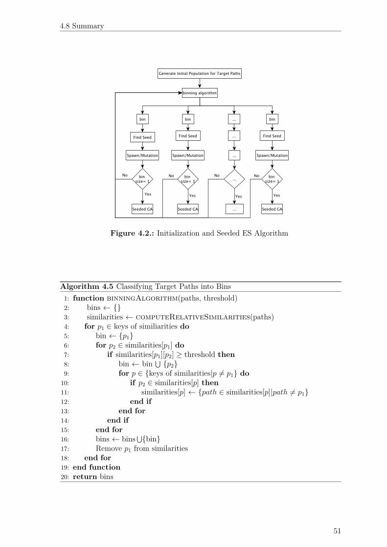
4.8 Summary
Figure 4.2.: Initialization and Seeded ES Algorithm
Algorithm 4.5 Classifying Target Paths into Bins1: function binningAlgorithm(paths, threshold)2: bins Ω {}3: similarities Ω computeRelativeSimilarities(paths)4: for p1 œ keys of similiarities do
5: bin Ω {p1}6: for p2 œ similarities[p1] do
7: if similarities[p1][p2] Ø threshold then
8: bin Ω bin t {p2}9: for p œ {keys of similarities|p ”= p1} do
10: if p2 œ similarities[p] then
11: similarities[p] Ω {path œ similarities[p]|path ”= p1}12: end if
13: end for
14: end if
15: end for
16: bins Ω bins t{bin}17: Remove p1 from similarities18: end for
19: end function
20: return bins
51
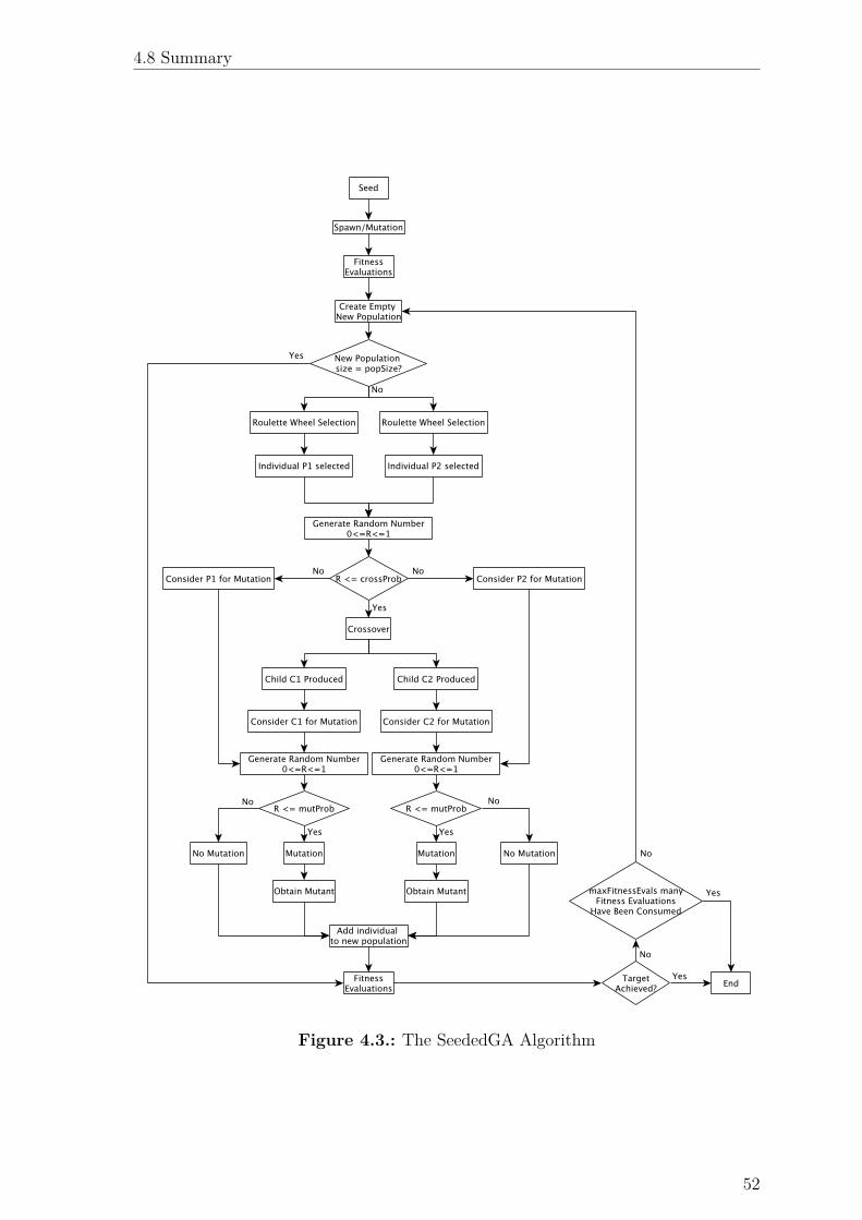
4.8 Summary
Figure 4.3.: The SeededGA Algorithm
52
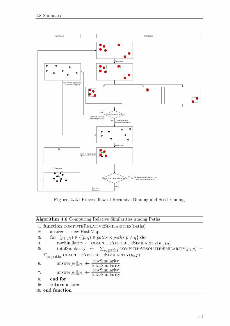
4.8 Summary
Figure 4.4.: Process flow of Recursive Binning and Seed Finding
Algorithm 4.6 Computing Relative Similarities among Paths1: function computeRelativeSimilarities(paths)2: answer Ω new HashMap3: for (p1, p2) œ {(p, q) œ paths ◊ paths|p ”= q} do
4: rawSimilarity Ω computeAbsoluteSimilarity(p1, p2)5: totalSimilarity Ω q
pœpaths computeAbsoluteSimilarity(p1,p) +q
pœpaths computeAbsoluteSimilarity(p2,p)
6: answer[p1][p2] Ω rawSimilaritytotalSimilarity
7: answer[p2][p1] Ω rawSimilaritytotalSimilarity
8: end for
9: return answer10: end function
53

4.8 Summary
Algorithm 4.7 Computing Absolute Similarities among Paths1: function computeAbsoluteSimilarity(p1, p2)2: matrix Ω computeSimilarityMatrix(p1, p2)3: return
max(matrix)maxlength(p1,p2)
4: end function
Algorithm 4.8 Computing Similarity Matrix1: function computeSimilarityMatrix(p1, p2)2: for i Ω 1 ... max(|p2| ≠ |p1|, 0) do
3: p1 Ω p1t NULL
4: end for
5: for i Ω 1 ... max(|p2| ≠ |p1|, 0) do
6: p2 Ω p2t NULL
7: end for
8: answer Ω0.0 . . . 0.0... . . . ...
0.0 . . . 0.0¸ ˚˙ ˝
|p1|
Z__̂
__\|p1|
9: for r Ω 1 ... |p1| ≠ 1 do
10: for c Ω 1 ... |p1| ≠ 1 do
11: if p1[r ≠ 1] == p2[c ≠ 1] then
12: answer[r][c] Ω answer[r-1][c-1] +113: else
14: answer[r][c] Ω 0.015: end if
16: end for
17: end for
18: return answer19: end function
54
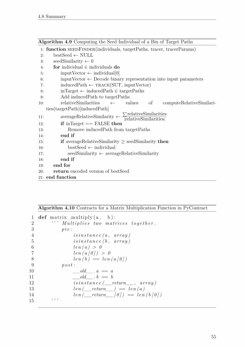
4.8 Summary
Algorithm 4.9 Computing the Seed Individual of a Bin of Target Paths1: function seedFinder(individuals, targetPaths, tracer, tracerParams)2: bestSeed Ω NULL3: seedSimilarity Ω 04: for individual œ individuals do
5: inputVector Ω individual[0]6: inputVector Ω Decode binary representation into input parameters7: inducedPath Ω trace(SUT, inputVector)8: inTarget Ω inducedPath œ targetPaths9: Add inducedPath to targetPaths
10: relativeSimilarities Ω values of computeRelativeSimilari-ties(targetPath)[inducedPath]
11: averageRelativeSimilarity Ωq relativeSimilarities|relativeSimilarities|
12: if inTarget == FALSE then
13: Remove inducedPath from targetPaths14: end if
15: if averageRelativeSimilarity Ø seedSimilarity then
16: bestSeed Ω individual17: seedSimilarity Ω averageRelativeSimilarity18: end if
19: end for
20: return encoded version of bestSeed21: end function
Algorithm 4.10 Contracts for a Matrix Multiplication Function in PyContract
1 def matrix_multiply ( a , b ) :2 ’ ’ ’ M u l t i p l i e s two matr ices t o g e t h e r .3 pre :4 i s i n s t a n c e (a , array )5 i s i n s t a n c e ( b , array )6 l en (a ) > 07 l en (a [ 0 ] ) > 08 l en ( b ) == len (a [ 0 ] )9 pos t :
10 __old__. a == a11 __old__. b == b12 i s i n s t a n c e (__return__ , array )13 l en (__return__) == len (a )14 l en (__return__ [ 0 ] ) == len ( b [ 0 ] )15 ’ ’ ’
55
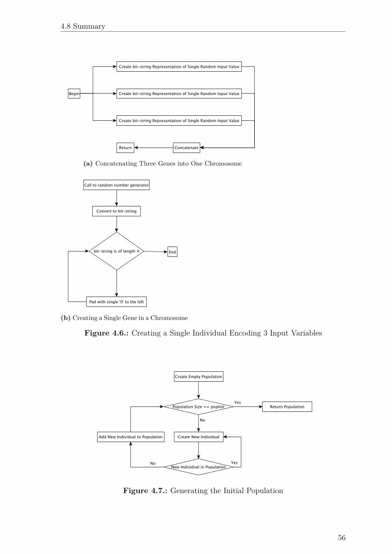
4.8 Summary
(a) Concatenating Three Genes into One Chromosome
(b) Creating a Single Gene in a Chromosome
Figure 4.6.: Creating a Single Individual Encoding 3 Input Variables
Figure 4.7.: Generating the Initial Population
56
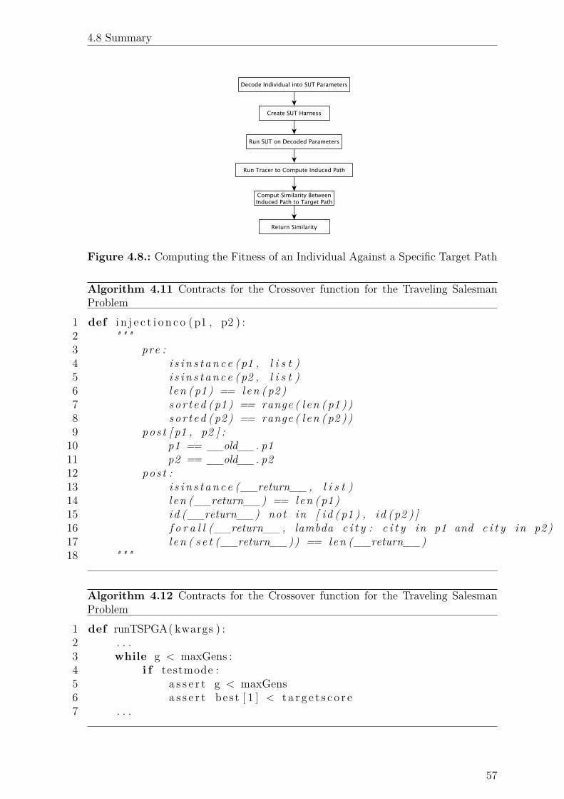
4.8 Summary
Figure 4.8.: Computing the Fitness of an Individual Against a Specific Target Path
Algorithm 4.11 Contracts for the Crossover function for the Traveling SalesmanProblem
1 def i n j e c t i o n c o (p1 , p2 ) :2 " " "3 pre :4 i s i n s t a n c e (p1 , l i s t )5 i s i n s t a n c e (p2 , l i s t )6 l en ( p1 ) == len ( p2 )7 so r t ed ( p1 ) == range ( l en ( p1 ))8 so r t ed ( p2 ) == range ( l en ( p2 ))9 pos t [ p1 , p2 ] :
10 p1 == __old__. p111 p2 == __old__. p212 pos t :13 i s i n s t a n c e (__return__ , l i s t )14 l en (__return__) == len ( p1 )15 i d (__return__) not in [ id ( p1 ) , id ( p2 ) ]16 f o r a l l (__return__ , lambda c i t y : c i t y in p1 and c i t y in p2 )17 l en ( s e t (__return__ )) == len (__return__)18 " " "
Algorithm 4.12 Contracts for the Crossover function for the Traveling SalesmanProblem
1 def runTSPGA( kwargs ) :2 . . .3 while g < maxGens :4 i f testmode :5 a s s e r t g < maxGens6 a s s e r t bes t [ 1 ] < t a r g e t s c o r e7 . . .
57
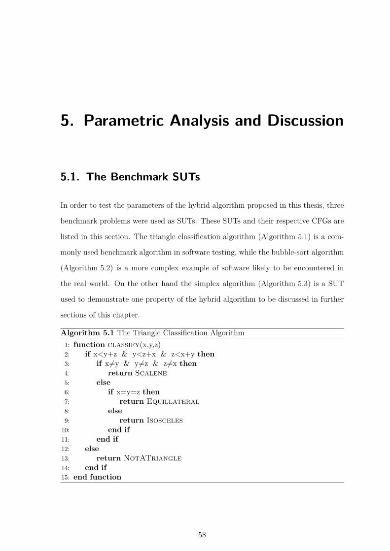
5. Parametric Analysis and Discussion
5.1. The Benchmark SUTs
In order to test the parameters of the hybrid algorithm proposed in this thesis, three
benchmark problems were used as SUTs. These SUTs and their respective CFGs are
listed in this section. The triangle classification algorithm (Algorithm 5.1) is a com-
monly used benchmark algorithm in software testing, while the bubble-sort algorithm
(Algorithm 5.2) is a more complex example of software likely to be encountered in
the real world. On the other hand the simplex algorithm (Algorithm 5.3) is a SUT
used to demonstrate one property of the hybrid algorithm to be discussed in further
sections of this chapter.
Algorithm 5.1 The Triangle Classification Algorithm1: function classify(x,y,z)2: if x<y+z & y<z+x & z<x+y then
3: if x”=y & y”=z & z ”=x then
4: return Scalene5: else
6: if x=y=z then
7: return Equillateral8: else
9: return Isosceles10: end if
11: end if
12: else
13: return NotATriangle14: end if
15: end function
58
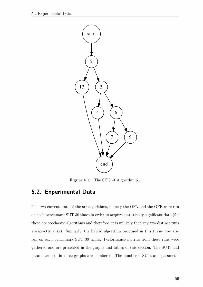
5.2 Experimental Data
start
2
end
13 3
4 6
7 9
Figure 5.1.: The CFG of Algorithm 5.1
5.2. Experimental Data
The two current state of the art algorithms, namely the OFA and the OFE were run
on each benchmark SUT 30 times in order to acquire statistically significant data (for
these are stochastic algorithms and therefore, it is unlikely that any two distinct runs
are exactly alike). Similarly, the hybrid algorithm proposed in this thesis was also
run on each benchmark SUT 30 times. Performance metrics from these runs were
gathered and are presented in the graphs and tables of this section. The SUTs and
parameter sets in these graphs are numbered. The numbered SUTs and parameter
59
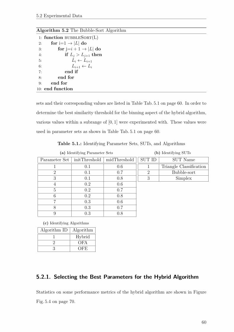
5.2 Experimental Data
Algorithm 5.2 The Bubble-Sort Algorithm1: function bubbleSort(L)2: for i=1 æ |L| do
3: for j=i + 1 æ |L| do
4: if Lj
> Lj+1 then
5: Li
Ω Li+1
6: Li+1 Ω L
i
7: end if
8: end for
9: end for
10: end function
sets and their corresponding values are listed in Table Tab. 5.1 on page 60. In order to
determine the best similarity threshold for the binning aspect of the hybrid algorithm,
various values within a subrange of [0, 1] were experimented with. These values were
used in parameter sets as shows in Table Tab. 5.1 on page 60.
Table 5.1.: Identifying Parameter Sets, SUTs, and Algorithms
(a) Identifying Parameter Sets
Parameter Set initThreshold midThreshold1 0.1 0.62 0.1 0.73 0.1 0.84 0.2 0.65 0.2 0.76 0.2 0.87 0.3 0.68 0.3 0.79 0.3 0.8
(b) Identifying SUTs
SUT ID SUT Name1 Triangle Classification2 Bubble-sort3 Simplex
(c) Identifying Algorithms
Algorithm ID Algorithm1 Hybrid2 OFA3 OFE
5.2.1. Selecting the Best Parameters for the Hybrid Algorithm
Statistics on some performance metrics of the hybrid algorithm are shown in Figure
Fig. 5.4 on page 70.
60
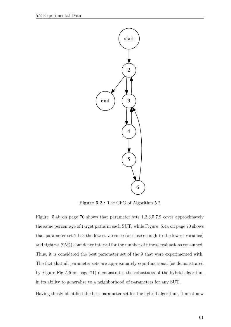
5.2 Experimental Data
start
2
end 3
4
5
6
Figure 5.2.: The CFG of Algorithm 5.2
Figure 5.4b on page 70 shows that parameter sets 1,2,3,5,7,9 cover approximately
the same percentage of target paths in each SUT, while Figure 5.4a on page 70 shows
that parameter set 2 has the lowest variance (or close enough to the lowest variance)
and tightest (95%) confidence interval for the number of fitness evaluations consumed.
Thus, it is considered the best parameter set of the 9 that were experimented with.
The fact that all parameter sets are approximately equi-functional (as demonstrated
by Figure Fig. 5.5 on page 71) demonstrates the robustness of the hybrid algorithm
in its ability to generalize to a neighborhood of parameters for any SUT.
Having thusly identified the best parameter set for the hybrid algorithm, it must now
61
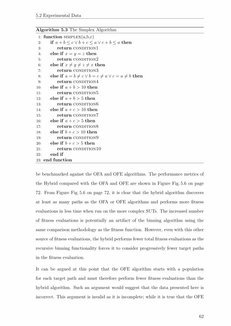
5.2 Experimental Data
Algorithm 5.3 The Simplex Algorithm1: function simplex(a,b,c)2: if a + b Æ c ‚ b + c Æ a ‚ c + b Æ a then
3: return condition14: else if x = y = z then
5: return condition26: else if x ”= y ”= z ”= x then
7: return condition38: else if a = b ”= c ‚ b = c ”= a ‚ c = a ”= b then
9: return condition410: else if a + b > 10 then
11: return condition512: else if a + b > 5 then
13: return condition614: else if a + c > 10 then
15: return condition716: else if a + c > 5 then
17: return condition818: else if b + c > 10 then
19: return condition920: else if b + c > 5 then
21: return condition1022: end if
23: end function
be benchmarked against the OFA and OFE algorithms. The performance metrics of
the Hybrid compared with the OFA and OFE are shown in Figure Fig. 5.6 on page
72. From Figure Fig. 5.6 on page 72, it is clear that the hybrid algorithm discovers
at least as many paths as the OFA or OFE algorithms and performs more fitness
evaluations in less time when run on the more complex SUTs. The increased number
of fitness evaluations is potentially an artifact of the binning algorithm using the
same comparison methodology as the fitness function. However, even with this other
source of fitness evaluations, the hybrid performs fewer total fitness evaluations as the
recursive binning functionality forces it to consider progressively fewer target paths
in the fitness evaluation.
It can be argued at this point that the OFE algorithm starts with a population
for each target path and must therefore perform fewer fitness evaluations than the
hybrid algorithm. Such an argument would suggest that the data presented here is
incorrect. This argument is invalid as it is incomplete; while it is true that the OFE
62
5.3 Properties of the Hybrid Algorithm
algorithm does start with each path being in its own bin (in the vernacular used
while describing the hybrid), each bin (containing a single target path) has its own
initial random population. This population occupies a large neighborhood, nor does it
converge quickly. On the other hand, the initial population of a seededGA algorithm
in the hybrid (the part of the hybrid algorithm invoked on singleton bins of target
paths ) densely occupies a small neighborhood. Further, it contains many duplicated
individuals, which leads to fewer distinct fitness function evaluations. Thus, the
observed behavior of the hybrid performing fewer fitness evalutions than the OFE
algorithm is not erroneous, but is a property of the hybrid algorithm itself.
5.3. Properties of the Hybrid Algorithm
5.3.1. Fewer Fitness Evaluations
As discussed in sec. 5.2.1, it is an expected property of the hybrid algorithm to perform
fewer fitness evaluations than the OFA and OFE algorithms. This is a desirable
property as it implies a faster turn around time in getting back results.
5.3.2. Local Optima
One of the problems faced by most stochastic algorithms is the di�culty of escaping
a local optimum. Indeed, this is a problem faced by the herein presented hybrid
algorithm as well. However, the e�ects of this problem on this algorithm are some-
what mitigated by the nature of the similarity measures used to compute the fitness
function. The fitness function computes the similarity of the path induced by an in-
dividual to the target path of that GA. Since there may be many input vectors (and
therefore many individuls) that could induce the target path, the GA is considered
to be working in a multi-modal fitness landscape. However, since all individuals that
induce the target path have the same fitness, discovering any of them would su�ce
as a termination condition.
63
5.3 Properties of the Hybrid Algorithm
The only remaining issue concerning local optima pertains to individuals, whose en-
odings represent a maximal (not maximum) fitness value (individuals that cannot
be made to induce paths that are more similar to the target path with only sim-
ple changes made to their encodings). However, due to the ESs ability to search
the neighborhood around the seed individual thoroughly, the GA is arguably primed
with a su�ciently diverse population that would allow for crossover and mutation
operations to facilitate the escape from local optima in the fitness landscape.
5.3.3. Parallelizability
In the recursive binning behavior of this hybrid algorithm, the recursive seededES and
seededGA steps are computed on each bin independently of the others. Therefore,
this hybrid algorithm is highly parallelizable. It is worth noting that this property is a
significant improvement over the OFA algorithm, which is no more parallelizable than
a classical GA. On the other hand, the OFE algorithm is also highly parallelizable,
but the hybrid requires demonstrably lower CPU time (as seen in Figure 5.6b on
page 72), which means that in a highly parallel system, it will still outperform the
OFE.
Further, due to the definition of the binning algorithm and its dependence on the
similarity threshold thereof, it is possible for the hybrid algorithm to generate sin-
gleton bins of target paths while simultaneously recursively classifying target paths
in other bins. In such situations, one CPU may compute the seededGA algorithm
on a singleton set of target paths, while another continues to recursively classify the
remaining target paths into bins. Thus, it is possible in few cases for the first CPU
to complete the computation of the seededGA algorithm before the second computes
the next singleton bin of target paths. This a�ord the hybrid algorithm the property
that even though it is approximately as parallel as the OFE algorithm, it does not
always require as many CPUs as the OFE in order to finish its computations. Indeed
the number of CPUs required by the OFE to be fully parallel is a tight upper bound
on the number of CPUs required by the hybrid algorithm to be fully parallel.
64
5.3 Properties of the Hybrid Algorithm
5.3.4. Inability to Stop Early
One of the observations from Figure 5.6c on page 72 and Figure 5.6b on page 72 is
that the hybrid algorithm performs poorly on the triangle classification SUT on the
elapsed runtime and number of fitness evaluations metrics. This is because, for very
simple SUTs, the inputs that induce the required target paths may exist in the initial
population. The OFA and OFE algorithms notice this and stop immediately. The
hybrid on the other hand, goes on to classify the target paths into bins, find a seed
for each bin and proceed with the rest of the algorithm until it does eventually find
the required individual that induces the target path. This is a shortcoming of the
hybrid algorithm. However, as seen in the various benchmarks in this section, this
shortcoming only applies to very small (almost trivial) SUTs, while the hybrid does
outperform both the OFA and the OFE in the more complex SUTs, to be expected
in the real world.
5.3.5. SUT Structure
The third benchmark SUT, namely the simplex algorithm is used to demonstrate one
of the properties of the hybrid algorithm. Indeed, this is a property of all evolutionary
algorithms that search for inputs that induce specific target paths. Recall from Figure
Fig. 4.4 on page 53 (repeated here for convenience in Figure Fig. 5.7 on page 73), that
the input vectors generated by the evolutionary algorithm are points in the input space
and the target paths that they are intended to induce are points in the path space. It
is therefore clear that the success of an evolutionary algorithm in discovering inputs
for target paths is a function of the semantic similarity between the two spaces. Thus,
an evolutionary algorithm will be more successful if a change of certain magnitude
and direction in the input space induces a change of similar magnitude and direction
in the path space. This is confirmed by the observation that all three algorithms (the
hydrid, OFA and OFE) perform consistently worse on the simplex SUT than they do
on the triangle classificaiton SUT. This is because small variations in the inputs to
65
5.4 A Real World SUT
each SUT cause varying changes in each SUT.
The triangle classification SUT is composed of highly nested if-then-else state-
ments, wherein the nested conditions are subsets of (or stronger conditions upon) the
parent condition. This implies that crossover and mutation operations have a high
probability of generating individuals that induce paths, nested one level higher or
lower than the the ones that the current individuals induce. This is particularly use-
ful when analysing locality and theoretically discussing and analyzing the progression
of the evolutionary algorithm over time.
However, the simplex SUT is specifically not structured this way. As a result, small
variations in an individual’s encoding can have very profound e�ects on the induced
path. This is to say that there is likely a larger distance between induced paths (in the
path space) of two individuals that are much closer in the input space. As a result,
the crossover and mutation operations do not have the desired localized exploration
properties for the simplex SUT that they do for the triangle classification SUT. This
is confirmed by the fact that all three evolutionary algorithms discovered more target
paths in the triangle classification SUT than in the simplex SUT1.
5.4. A Real World SUT
Having surpassed the other algorithms on classical benchmarking SUTs, the hybrid
was benchmarked against the OFA and OFE algorithms using a Hu�man encoder as
a SUT. The code and the CFG (of the implementation) for this SUT are shown in
Algorithm 5.4, Algorithm 5.5, Algorithm 5.6, Algorithm 5.7 and Figure Fig. 5.8 on
page 74.
Clearly, this is a more complex SUT and can well be expected to be found in the real
world. It was found that the hybrid algorithm outperformed both the OFA and the
OFE algorithms on the following metrics:
• percentage of target paths discovered1see Section sec. 6.3 for how to deal with this problem
66
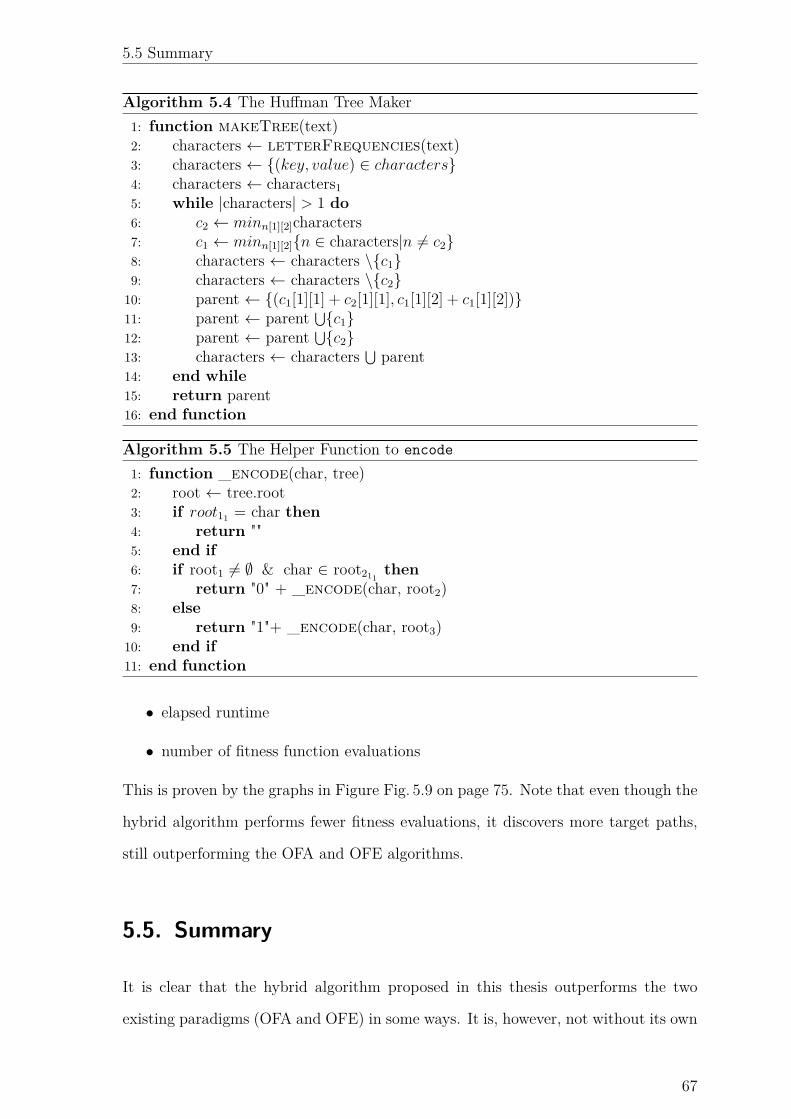
5.5 Summary
Algorithm 5.4 The Hu�man Tree Maker1: function makeTree(text)2: characters Ω letterFrequencies(text)3: characters Ω {(key, value) œ characters}4: characters Ω characters15: while |characters| > 1 do
6: c2 Ω minn[1][2]characters
7: c1 Ω minn[1][2]{n œ characters|n ”= c2}
8: characters Ω characters \{c1}9: characters Ω characters \{c2}
10: parent Ω {(c1[1][1] + c2[1][1], c1[1][2] + c1[1][2])}11: parent Ω parent t{c1}12: parent Ω parent t{c2}13: characters Ω characters t parent14: end while
15: return parent16: end function
Algorithm 5.5 The Helper Function to encode
1: function _encode(char, tree)2: root Ω tree.root3: if root11 = char then
4: return ""5: end if
6: if root1 ”= ÿ & char œ root211then
7: return "0" + _encode(char, root2)8: else
9: return "1"+ _encode(char, root3)10: end if
11: end function
• elapsed runtime
• number of fitness function evaluations
This is proven by the graphs in Figure Fig. 5.9 on page 75. Note that even though the
hybrid algorithm performs fewer fitness evaluations, it discovers more target paths,
still outperforming the OFA and OFE algorithms.
5.5. Summary
It is clear that the hybrid algorithm proposed in this thesis outperforms the two
existing paradigms (OFA and OFE) in some ways. It is, however, not without its own
67

5.5 Summary
Algorithm 5.6 The Encoding Function1: function encode(text, tree)2: answer Ω {}3: for char d œ text do
4: cipher Ω _encode(char, tree)5: answer Ω answer t{cipher}6: end for
7: return string(answer)8: end function
Algorithm 5.7 Main1: function main(text)2: tree Ω makeTree(text)3: return encode(text, tree)4: end function
shortcommings, such as its inability to stop early, etc (outlined in sec. 5.3), which are
promising areas for future work.
68
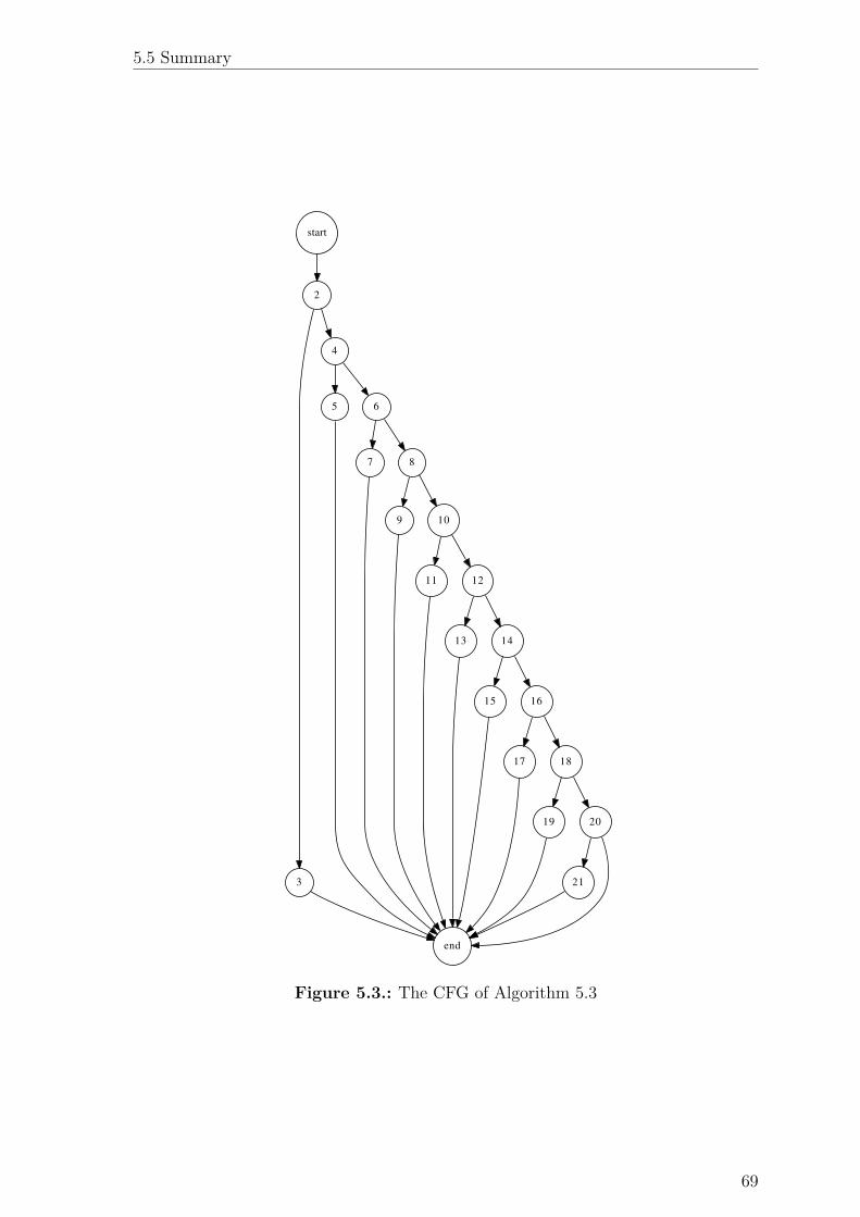
5.5 Summary
start
2
end
3
4
5 6
7 8
9 10
11 12
13 14
15 16
17 18
19 20
21
Figure 5.3.: The CFG of Algorithm 5.3
69
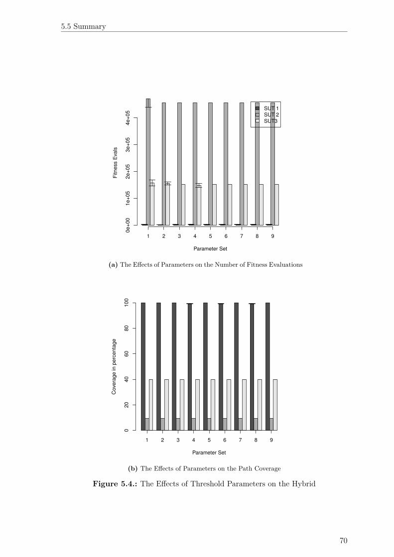
5.5 Summary
1 2 3 4 5 6 7 8 9
SUT 1
SUT 2
SUT3
Parameter Set
Fitn
ess E
va
ls
0e
+0
01
e+
05
2e
+0
53
e+
05
4e
+0
5
(a) The E�ects of Parameters on the Number of Fitness Evaluations
1 2 3 4 5 6 7 8 9
Parameter Set
Cove
rag
e in
pe
rce
nta
ge
02
04
06
08
01
00
(b) The E�ects of Parameters on the Path Coverage
Figure 5.4.: The E�ects of Threshold Parameters on the Hybrid
70
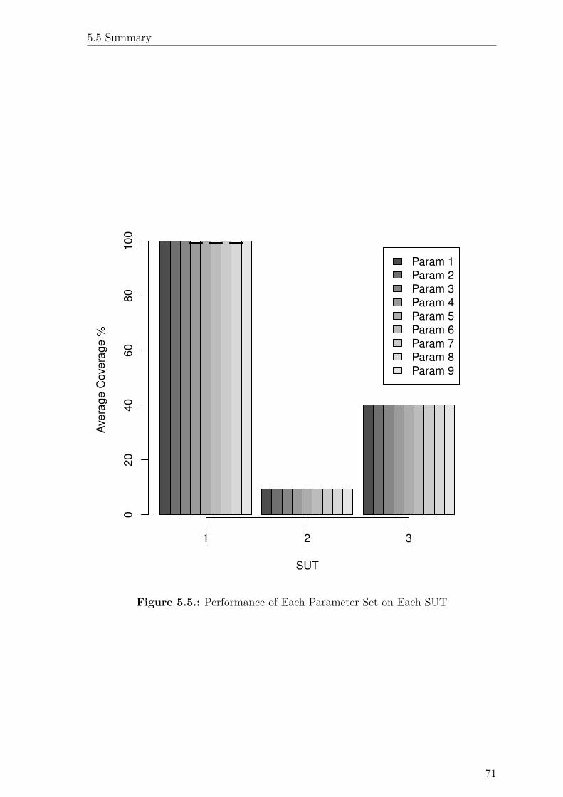
5.5 Summary
1 2 3
Param 1Param 2Param 3Param 4Param 5Param 6Param 7Param 8Param 9
SUT
Ave
rage C
ove
rage
%
020
40
60
80
100
Figure 5.5.: Performance of Each Parameter Set on Each SUT
71
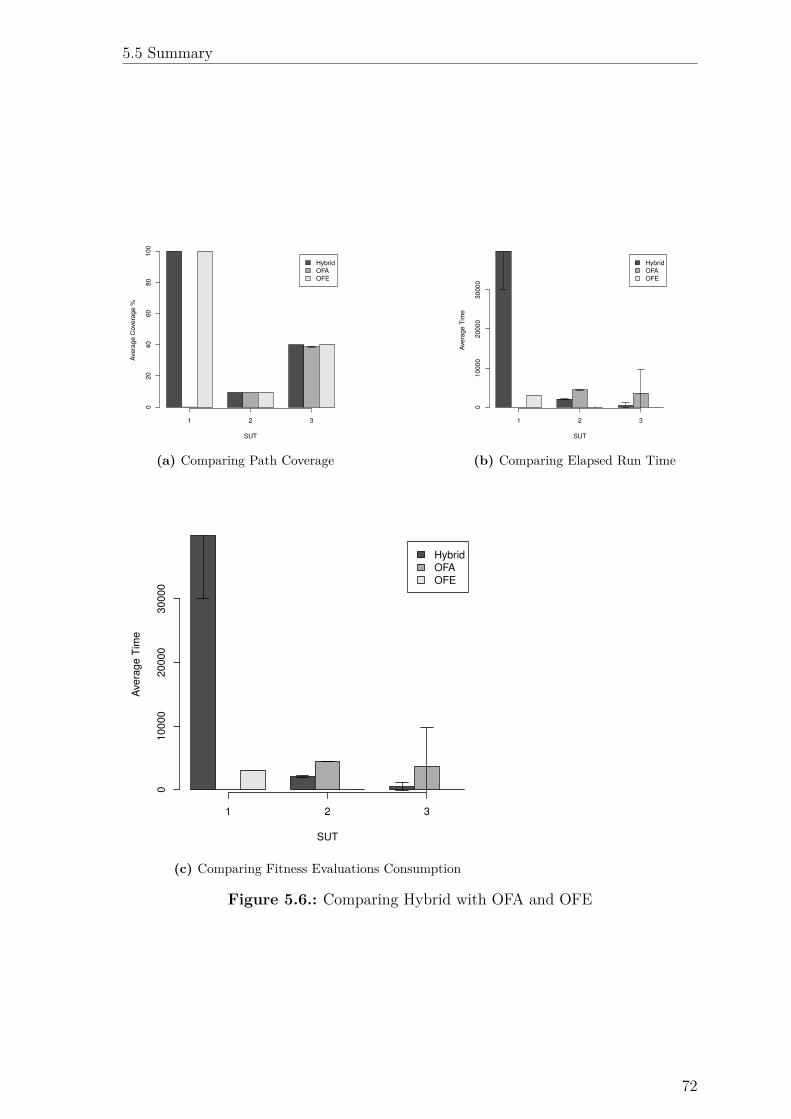
5.5 Summary
1 2 3
HybridOFAOFE
SUT
Ave
rag
e C
ove
rag
e %
02
04
06
08
01
00
(a) Comparing Path Coverage
1 2 3
HybridOFAOFE
SUT
Ave
rag
e T
ime
01
00
00
20
00
03
00
00
(b) Comparing Elapsed Run Time
1 2 3
HybridOFAOFE
SUT
Ave
rag
e T
ime
01
00
00
20
00
03
00
00
(c) Comparing Fitness Evaluations Consumption
Figure 5.6.: Comparing Hybrid with OFA and OFE
72
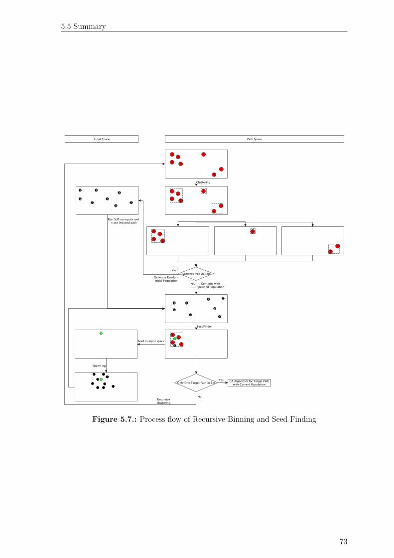
5.5 Summary
Figure 5.7.: Process flow of Recursive Binning and Seed Finding
73
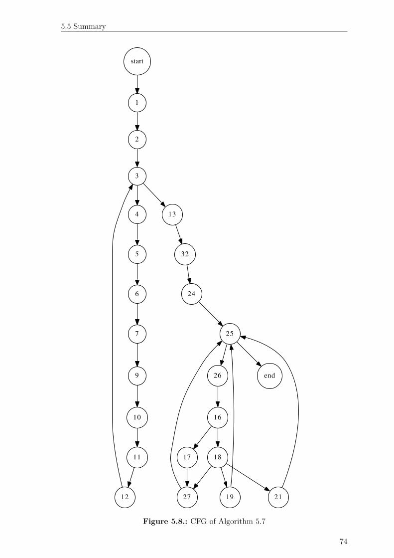
5.5 Summary
start
1
end
2
3
4 13
5 32
6
7
9
10
11
12
24
17
27
25
26
16
18
19 21
Figure 5.8.: CFG of Algorithm 5.7
74
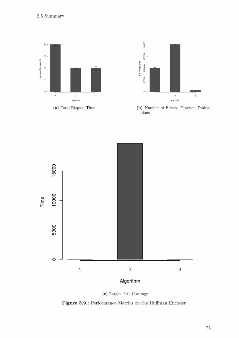
5.5 Summary
1 2 3
Algorithm
Ave
rag
e C
ove
rag
e %
05
10
15
20
(a) Total Elapsed Time
1 2 3
Algorithm
# o
f F
itne
ss E
vals
05
00
00
01
00
00
00
15
00
00
02
00
00
00
(b) Number of Fitness Function Evalua-tions
1 2 3
Algorithm
Tim
e
05000
10000
15000
(c) Target Path Coverage
Figure 5.9.: Performance Metrics on the Hu�man Encoder
75
6. Conclusions and Future Work
6.1. Overview
As discussed in chapter 5, the hybrid algorithm proposed in this thesis is indeed
an improvement over the OFA and OFE algorithms. Further, since the preliminary
results of this thesis have been peer reviewed [23], it is accurate to claim that this
thesis presents a new solution to the studied problem, which outperforms the current
state of the art.
Further, chapter 5 shows that this algorithm works well for classification algorithms
(the triangle classification algorithm), sorting algorithm (the bubble-sort algorithm),
comparison algorithms (the simplex algorithm) and transformation algorithms (the
Hu�man encoding algorithm). These algorithms together form somewhat a spanning
set of the operations found in most modern deterministic software. Thus, it is logical
to conclude that good performance on these SUTs will yield similarly good perfor-
mance on real world SUTs composed of similar SUTs. Thus, it is expected that the
hybrid algorithm presented in this thesis will generalize well to most software in the
real world.
6.2. Summary of Contributions
This thesis presents a hybrid evolutionary algorithm, comprised of a Genetic Algo-
rithm (GA) and an Evolutionary Strategy (ES). It is the purpose of the ES to shape
76
6.3 Future Work
the evolutionary population in such a way as to aid the GA by providing an ad-
equately diverse population in a neigborhood suspected of harboring a su�ciently
fit individual. When applied to a problem such as path coverage in software test-
ing (which is represented in a multi-modal fitness landscape), this hybrid algorithm
outperforms the current state of the art.
6.3. Future Work
It is worth noting that only deterministic software was used at SUTs in the results
presented in this thesis. It is therefore not guaranteed to perform comparably on non-
deterministic SUTs such as evolutionary algorithms, neural networks, etc. However,
it is acceptable to expect it to perform comparably on non-deterministic software that
uses a random seed for testing purposes. This is a useful avenue to pursue for future
work, as it would bring with it, the ability to test the software written for this thesis
itself.
Further, the hybrid algorithm could be improved upon by including the ability to
remove target paths from consideration if individuals that induce them have already
been generated; even before singleton bins of target paths are computed. This would
increase the e�ciency of the algorithm, especially in the cases of simpler SUTs such
as the triangle classification SUT.
Another possible improvement combines principles from static software testing and
compiler optimization technology that reorders lines of code [24]. Since the struc-
ture of the conditional statements does have an impact on the performance of the
algorithm, a system that performs static analysis to compute the predicates on each
line of code and subsequently reorder the lines of code in order to nest the predicates
themselves, would yield an improvement in the performance of the hybrid algorithm
as a whole. As mentioned in Chapter chapter 5, this is one of the reasons for the poor
performance of the hybrid algorithm on the simplex SUT.
The final improvement takes advantage of automated bug reporting systems such as
77

6.3 Future Work
those used by modern web browsers [25] to automatically determine what target paths
need to be tested with high priority. Thus, the hybrid algorithm can automatically
be tasked with discovering inputs for that particular target path to generate a more
detailed bug report for the developers of the SUT.
78
Appendix A.
The CFG Package
A.1. Motivation
The CFG (Control Flow Graph) package is designed to extract a CFG out of the
source code for a given SUT. Given that the SUT in this thesis is written in Python,
this is accomplished with the cfg package [26], presented in this appendix.
A.2. Overview
There are existing packages for the python programming language that compute a
call graph for the given source-code [27]. However, these packages do not allow for
extracting a CFG out of the source-code, despite the fact that they likely use such
a CFG internally. Further, the python interpreter itself (written in C) [28] converts
the source-code into a CFG, as an intermediary step in converting source-code into
machine code. However, this is done “on the fly” and therefore is not accessible either.
Thus, the cfg package was created and used in this thesis.
Since python is an interpreted language, it is possible to use built-in methods [29] to
obtain its AST (Abstract Syntax Tree). It is from this AST that the CFG is built.
Since the AST is tree data structure that contains pointers from parent nodes to child
79
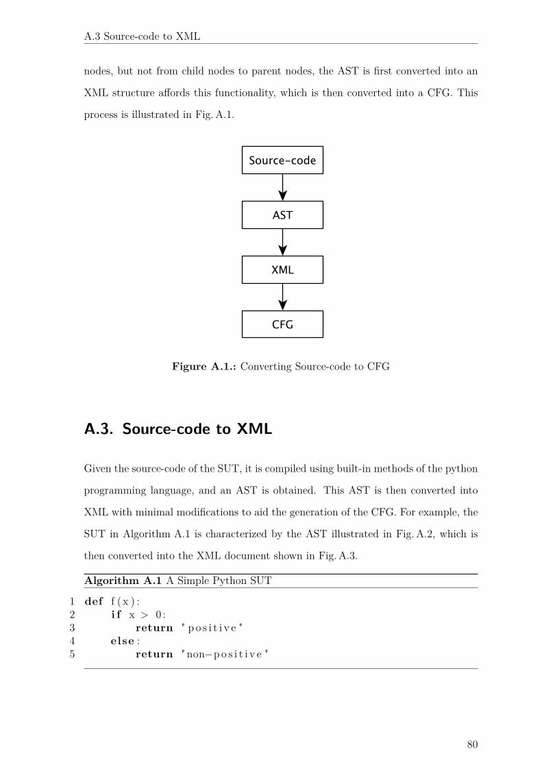
A.3 Source-code to XML
nodes, but not from child nodes to parent nodes, the AST is first converted into an
XML structure a�ords this functionality, which is then converted into a CFG. This
process is illustrated in Fig. A.1.
Figure A.1.: Converting Source-code to CFG
A.3. Source-code to XML
Given the source-code of the SUT, it is compiled using built-in methods of the python
programming language, and an AST is obtained. This AST is then converted into
XML with minimal modifications to aid the generation of the CFG. For example, the
SUT in Algorithm A.1 is characterized by the AST illustrated in Fig. A.2, which is
then converted into the XML document shown in Fig. A.3.
Algorithm A.1 A Simple Python SUT
1 def f ( x ) :2 i f x > 0 :3 return " p o s i t i v e "4 else :5 return " non≠p o s i t i v e "
80

A.3 Source-code to XML
This XML is converted into a CFG. Since the general algorithm is too large to be
shown here, only the sections necessary to handle this XML is shown in Algorithm A.2.
Ultimately, once the parse function has finished execution, a CFG is created. This
CFG holds a representation of the graph shown in Fig. A.4.
81

A.3 Source-code to XML
Figure A.2.: The AST of Algorithm A.1
82
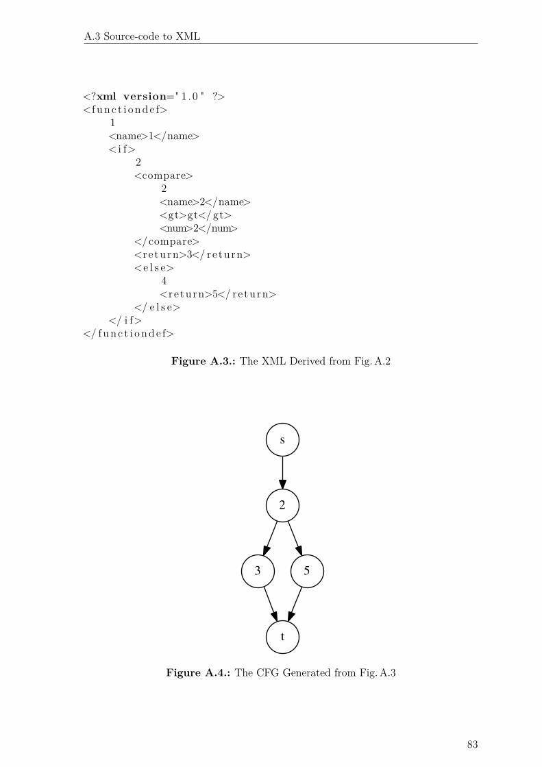
A.3 Source-code to XML
<?xml version=" 1 .0 " ?><func t i onde f>
1<name>1</name>< i f>
2<compare>
2<name>2</name><gt>gt</ gt><num>2</num>
</compare><return>3</ return><e l s e>
4<return>5</ return>
</ e l s e></ i f>
</ func t i onde f>
Figure A.3.: The XML Derived from Fig. A.2
s
2
t
3 5
Figure A.4.: The CFG Generated from Fig. A.3
83

A.3 Source-code to XML
Algorithm A.2 Converting Fig. A.3 to a CFG1: class xmlToCFG2: function initialize(xmlFilePath)3: Û ‘self‘ describes the object itself, similar to ‘this‘ in Java4: self.xml Ω root of the XML document5: self.edges Ω new HashMap6: self.last Ω line number of root7: self.currScope Ω new array8: self.funcstarts Ω ÿ9: end function
10: function parse11: self.scopes Ω self.scopes t{(0, largest line number in the XML)}12: self.handleNode(self.xml)13: end function
14: function handleNode(node)15: curr Ω line number of node16: if curr ”œ self.last then
17: for last in self.last do
18: add curr as an outgoing edge from last19: remove last from self.last20: end for
21: end if
22: add curr to self.last23: self.HANDLERS[node.tag](node)24: end function
25: function handleIf(node)26: elseblock Ω last child of node27: add the line number of the first child of elseblock as an outgoing node from
elseblock28: for child œ { children of node | child ”= elseblock } do
29: self.handleNode(child)30: end for
31: cache Ω memcpy(self.last)32: add the line number of node to self.last33: remove line numbers of all child nodes from self.last34: for child œ children of elseblock do
35: self.handleNode(child)36: end for
37: add the line number of the last line of node to self.last38: self.last Ω self.last t cache39: end function
40: function handleCondition(node)41: for child œ children of node do
42: self.handleNode(child)43: end for
44: end function
45: function handleReturn(node)46: for child œ children of node do
47: self.handleNode(child)48: end for
49: end function
50: end class 84
Appendix B.
Dynamic White Box Testing
B.1. Overview
White box testing is a software testing paradigm that uses the source code of the SUT
to test it. It is used to ensure that all parts of the code’s structure are executable
- to ensure code coverage. As such, there are several forms of white-box testing. In
each form, the SUT is converted into a control flow graph (CFG) - a mathematical
representation of the logical program flow of the SUT. In a CFG, each statement
is a node and sequential statements are connected by edges. Branching statements
(if-then-else statements, for-loops and while-loops) are characterized by mul-
tiple outgoing edges from a node, with conditions on each edge.
B.2. Node or Statement Coverage
This form of white box testing requires that each statement in the SUT’s code be
executed by at least one input vector from the set of test input vectors. While
this seems acceptable, it is trivial to show that this testing method is incomplete.
Consider the following example of a program that is said to implement the following
specifications:
85
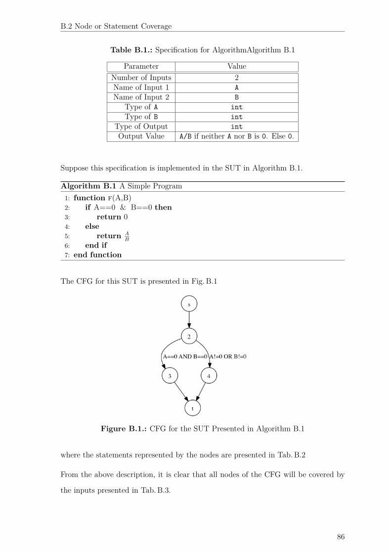
B.2 Node or Statement Coverage
Table B.1.: Specification for AlgorithmAlgorithm B.1
Parameter ValueNumber of Inputs 2Name of Input 1 A
Name of Input 2 B
Type of A int
Type of B int
Type of Output int
Output Value A/B if neither A nor B is 0. Else 0.
Suppose this specification is implemented in the SUT in Algorithm B.1.
Algorithm B.1 A Simple Program1: function f(A,B)2: if A==0 & B==0 then
3: return 04: else
5: return
A
B
6: end if
7: end function
The CFG for this SUT is presented in Fig. B.1
Figure B.1.: CFG for the SUT Presented in Algorithm B.1
where the statements represented by the nodes are presented in Tab. B.2
From the above description, it is clear that all nodes of the CFG will be covered by
the inputs presented in Tab. B.3.
86

B.3 Edge Coverage
Table B.2.: Node-Statement Representation
Node Statement
s Start function2 if (A == 0) AND (B == 0)
3 return 0
4 return A/B
t End function
Table B.3.: Inputs for Node Coverage
A B Path
0 0 (s,2,3,t)0 1 (s,2,4,t)
Having covered all nodes of the SUT, the test suite comprised of the input vectors
presented in Tab. B.3 would declare the SUT bug-free. However, note that the input
vector (A=1, B=0) was not tested and would cause an error due to division-by-zero.
This is an error case, that is not caught by the test suite which declared this code to
be bug-free.
Thus, node coverage is not an adequate code coverage criterion for testing
B.3. Edge Coverage
Edge coverage is a stronger testing criterion than node coverage [6]. Similar to node
coverage, edge coverage attempts to execute all edges in the SUT’s code. This is to
say that a test suite T satisfies edge coverage if and only if for every edge e in the
CFG of the SUT, there exists a test case (i.e. a vector of inputs) t œ T such that the
path induced by executing the SUT on t contains e.
Using the same example as in sec. B.2, we can see that edge coverage is also incom-
plete. The two input vectors in the test suite, together cover all edges. Still, they miss
the fact that the input vector (A=1, B=0) would cause an error due to division-by-zero.
87
B.4 Condition Coverage
B.4. Condition Coverage
Condition coverage is a stronger testing criterion than edge coverage [6]. This criterion
requires that every condition that can induce a path of execution in the SUT be
executed at least once by the test suite [6]. This is to say that a test suite T satisfies
condition coverage if and only if for each set of path predicates P in the paths of the
CFG of the SUT, there exists a test case (i.e. a vector of inputs) t œ T such that the
path induced by executing the SUT on t contains P .
However, in the above SUT, it is clear that this criterion is incomplete, just as the
edge coverage criterion is also incomplete. Since condition coverage is satisfied by the
test suite presented in sec. B.2, and that test suite has been shown to be incomplete,
condition coverage is also incomplete.
B.5. Path Coverage
Path coverage is one of the stronger testing criteria1, and is widely accepted as a
natural criterion of program testing completeness [8]. It requires that every path in
the CFG be executed at least once by the test suite. This is true despite the fact
that the presented test suite satisfies this criterion . As a result, this thesis focuses
on generating input vectors that satisfy path coverage. It is left to the tester of the
software to determine what percentage of all paths in the CFG need to be induced
by the inputs generated by the work presented in this thesis.
1See for background information on the di�erent forms of coverage in white-box testing
88
Appendix C.
Evolutionary Algorithms
C.1. Genetic Algorithms
C.1.1. Overview
As outlined by Juang [30], a Genetic Algorithm (GA) encodes a candidate solution
to a problem in an individual of a population of such individuals. These indivuals
are composed of chromosomes, which encode parts of the candidate solution. After
initializing a random population of such individuals, these are evaluated for fitness
(i.e. a measure determining the optimality of the candidate solution in its ability
to solve the problem). Fit individuals are reproduced to the next generation of the
population. Further, all members of the current generation of the population undergo
probabilistic crossover and mutation operations so that parts of candidate solutions
may be combined with each other in the hope of creating a better individual (i.e. a
candidate solution) for the next generation. This process of reproduction, crossover
and mutation operations are repeated for several generations over a run of the GA.
The various components of a GA are explained in the following subsections.
89
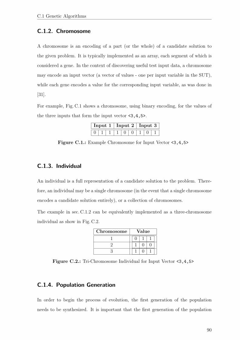
C.1 Genetic Algorithms
C.1.2. Chromosome
A chromosome is an encoding of a part (or the whole) of a candidate solution to
the given problem. It is typically implemented as an array, each segment of which is
considered a gene. In the context of discovering useful test input data, a chromosome
may encode an input vector (a vector of values - one per input variable in the SUT),
while each gene encodes a value for the corresponding input variable, as was done in
[31].
For example, Fig. C.1 shows a chromosome, using binary encoding, for the values of
the three inputs that form the input vector <3,4,5>.
Input 1 Input 2 Input 3
0 1 1 1 0 0 1 0 1
Figure C.1.: Example Chromosome for Input Vector <3,4,5>
C.1.3. Individual
An individual is a full representation of a candidate solution to the problem. There-
fore, an individual may be a single chromosome (in the event that a single chromosome
encodes a candidate solution entirely), or a collection of chromosomes.
The example in sec. C.1.2 can be equivalently implemented as a three-chromosome
individual as show in Fig. C.2.
Chromosome Value
1 0 1 12 1 0 03 1 0 1
Figure C.2.: Tri-Chromosome Individual for Input Vector <3,4,5>
C.1.4. Population Generation
In order to begin the process of evolution, the first generation of the population
needs to be synthesized. It is important that the first generation of the population
90
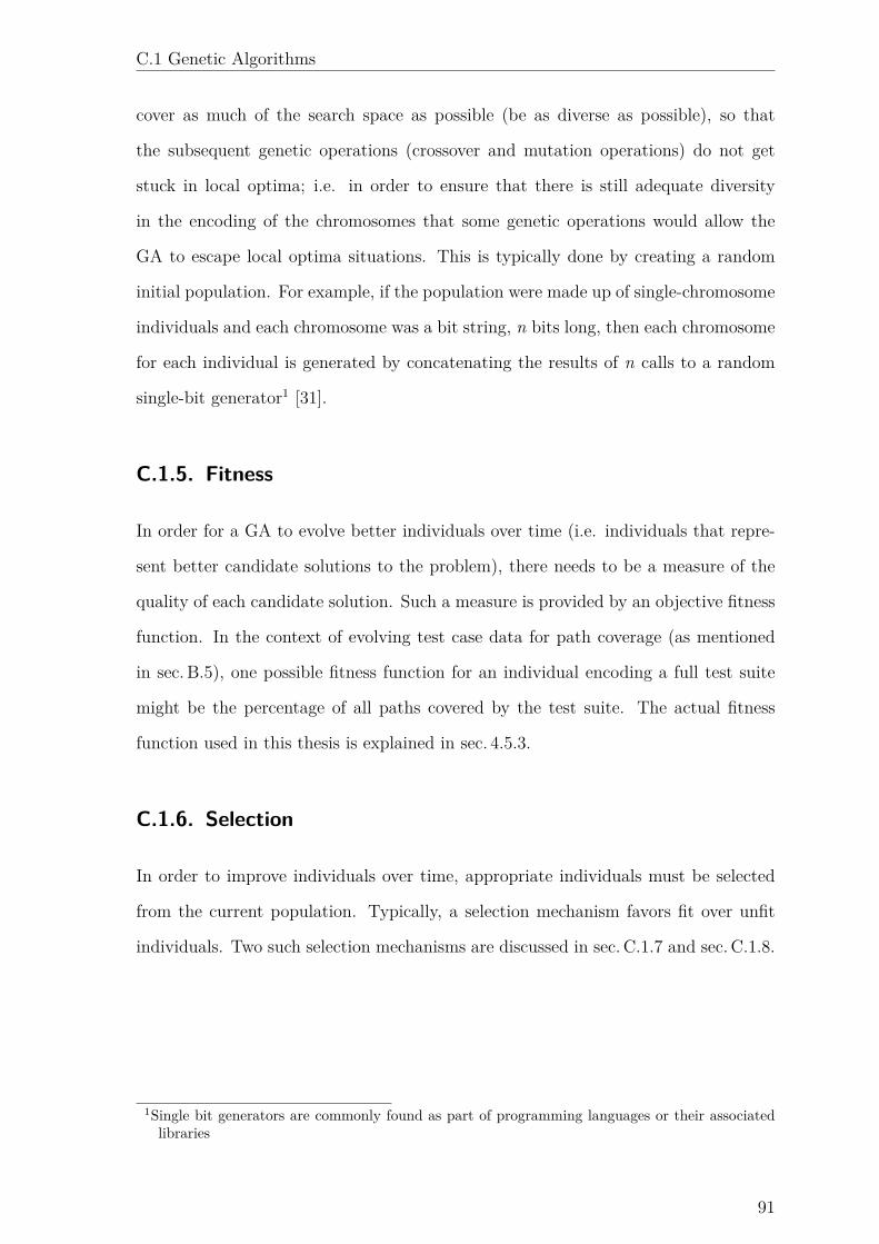
C.1 Genetic Algorithms
cover as much of the search space as possible (be as diverse as possible), so that
the subsequent genetic operations (crossover and mutation operations) do not get
stuck in local optima; i.e. in order to ensure that there is still adequate diversity
in the encoding of the chromosomes that some genetic operations would allow the
GA to escape local optima situations. This is typically done by creating a random
initial population. For example, if the population were made up of single-chromosome
individuals and each chromosome was a bit string, n bits long, then each chromosome
for each individual is generated by concatenating the results of n calls to a random
single-bit generator1 [31].
C.1.5. Fitness
In order for a GA to evolve better individuals over time (i.e. individuals that repre-
sent better candidate solutions to the problem), there needs to be a measure of the
quality of each candidate solution. Such a measure is provided by an objective fitness
function. In the context of evolving test case data for path coverage (as mentioned
in sec. B.5), one possible fitness function for an individual encoding a full test suite
might be the percentage of all paths covered by the test suite. The actual fitness
function used in this thesis is explained in sec. 4.5.3.
C.1.6. Selection
In order to improve individuals over time, appropriate individuals must be selected
from the current population. Typically, a selection mechanism favors fit over unfit
individuals. Two such selection mechanisms are discussed in sec. C.1.7 and sec. C.1.8.
1Single bit generators are commonly found as part of programming languages or their associatedlibraries
91

C.1 Genetic Algorithms
C.1.7. Biased Roulette Wheel Selection
A biased roulette wheel selection models a situation where individuals bet on a
roulette wheel, and the winner will be chosen for reproduction (crossover and muta-
tion) operations. In order to bias the bets that the individuals place, each individual
is to bet on an entire section of the roulette wheel. The size of the section is directly
proportional to the fitness of the individual, relative to the population [8]. For ex-
ample, if a population consists of three individuals whose fitness scores are as shown
in Tab. C.1, the biased roulette wheel could be modeled along the continuous interval
[0, 1], for the individuals to place bets as shown in Tab. C.2.
Table C.1.: Relative Fitness of Individuals in a Population
Individual Raw Fitness Relative Fitness2
1 5 0.52 1 0.13 4 0.4
Table C.2.: A Biased Roulette-Wheel for the Individuals in Table Tab. C.1
Individual Section of the Roulette Wheel
1 0.0 - 0.52 0.5 - 0.63 0.6 - 1.0
After creating the biased roulette wheel and assigning sections for each individual
to place bets on, a selection operation is performed by picking a random number
in the interval. The individual that placed a bet on a section of the roulette wheel
containing this random number is determined to be the winner. Thus if the random
number was 0.506934, then Individual 2 is selected for mating operations.
C.1.8. Tournament Selection
A tournament selection is based on of the following parameters:
Tournament size (T) The size of the tournament to be conducted
92

C.1 Genetic Algorithms
Number of winners (W) The number of winners of a tournament. Typically, this is
either 1 or 2; this number has a lower bound of 1 and an upper bound of T
This selection mechanism functions by sampling T individuals from the population
and selecting the best (fittest) W of them for mating operations [32]. The idea is
that fitter individuals have a higher probability of mating to produce children, which
will populate the next generation of the population of chromosomes. Note that this
selection mechanism guarantees that the T ≠W least fit individuals in any generation
of the population will never be selected for reproduction operations.
Thus, while this method is another way to implement fitness-proportional selection,
it is less forgiving that the biased roulette wheel selection mechanism, as a biased
roulette wheel does not make it impossible for the least fit T ≠ W individuals to be
selected for reproduction operations (even though this probability will be very low in
a biased roulette-wheel selection).
C.1.9. Crossover
In order to combine components of known candidate solutions to form new candidate
solutions, a process named crossover is employed. During crossover, corresponding
parts of corresponding pairs of chromosomes from two parent individuals are recom-
bined to form the chromosomes of the child individual. While several methods for
crossover do exist and are used, two are examined in sec. C.1.9.1 and sec. C.1.9.2.
C.1.9.1. Uniform Crossover
Uniform crossover generates a child chromosome in which each gene is a copy of the
corresponding gene in one of the parents. Which parent a particular gene comes from
is decided probabilistically. For example, suppose:
1. the two parents (p1 and p2) were as shown in Figure C.3a on page 94
2. the probability of selecting a gene from p2 is 0.5
93

C.1 Genetic Algorithms
Then, the probability of the first gene in the child from crossover being A2 is 0.5.
Thus, the probability of generating the child shown in C.3b as a result of crossover
is 0.0625.
p1 A1 B1 C1 D1p2 A2 B2 C2 D2
(a) Hypothetical Parents ofCrossover
Child A1 B2 C1 D2
(b) Possible Child of Crossover
Figure C.3.: Uniform Crossover Example
Indeed, the probability of generating one of the parents as a result of crossover is
also 0.0625. This crossover technique was used in generating test inputs for testing a
vehicular cruise control system [31].
C.1.9.2. One Point Crossover
One point crossover generates a child chromosome by concatenating complement seg-
ments of corresponding chromosomes of the parent individuals. The point of segmen-
tation (called the crossover point) is selected at random. For example, suppose the
two parents (p1 and p2) were as shown in Figure C.3a on page 94, it is possible that a
child chromosome would be (if the crossover point were between the third and fourth
gene) as shown in Fig. C.4.
Child A1 B1 C1 D2
Figure C.4.: Possible Child of One-Point Crossover
C.1.10. Mutation
Mutation is a process by which a chromosome is altered slightly in order to create
a variant of itself. This is done in order to allow the GA to escape local optima by
allowing the chromosome, hence the individual, to move to a di�erent point in the
solution space. For example, if a chromosome is represented as a binary bit-string, a
mutation operation would flip the value of a random bit in this bit-string. This can
be observed in the fourth gene in Fig. C.5.
94

C.2 Evolutionary Strategy
Before Mutation 0 1 0 0After Mutation 0 1 0 1
Figure C.5.: Possible Mutation
C.2. Evolutionary Strategy
An Evolutionary Strategy (ES) is an evolutionary algorithm similar to a GA. The
main di�erence is that ESs do not use crossover operators. Instead, once the initial
random population has been generated, it then advances from one generation to the
next by selecting the fittest individual of that generation and mutating it several
times in order to form the individuals of the next generation of that population. This
is performed over several generations, to execute one run of the ES.
95
Bibliography
[1] B. Jones, H.-H. Sthamer, and D. Eyres, “Automatic structural testing using
genetic algorithms,” Software Engineering Journal, vol. 11, no. 5, p. 299, 1996.
[Online]. Available: http://digital-library.theiet.org/content/journals/10.1049/
sej.1996.0040
[2] P. Neumann, “Mariner I – no holds BARred,” The Risks Digest, vol. 8, no. 75,
1989.
[3] B. Korel, “Automated Software Test Data Generation,” IEEE TRANSAC-
TIONS ON SOFTWARE ENGINEERING, vol. 16, no. 8, pp. 870–879,
1990. [Online]. Available: http://www-public.it-sudparis.eu/~gibson/Teaching/
CSC7302/ReadingMaterial/Korel90.pdf
[4] T. Ostrand, “Black-Box Testing,” Encyclopedia of Software Engineering, 2002.
[Online]. Available: http://onlinelibrary.wiley.com/doi/10.1002/0471028959.
sof022/abstract;jsessionid=DEE32EFE3BF956D043E4E0D086E66591.d01t01?
deniedAccessCustomisedMessage=&userIsAuthenticated=false
[5] E. Dustin, J. Rashka, and J. Paul, Automated software testing: introduction,
management, and performance. Addison-Wesley Professional, 1999.
[6] M. a. Ahmed and I. Hermadi, “GA-based multiple paths test data
generator,” Computers & Operations Research, vol. 35, no. 10, pp. 3107–3124,
Oct. 2008. [Online]. Available: http://linkinghub.elsevier.com/retrieve/pii/
S0305054807000251
[7] G. J. Myers, “The art of software testing, Publication info.”
96
Bibliography
[8] M. Pei, E. D. Goodman, Z. Gao, and K. Zhong, “Automated software test data
generation using a genetic algorithm,” Michigan State University, Tech. Rep,
no. 1, pp. 1–15, 1994.
[9] C. S. Pasareanu, N. Rungta, and W. Visser, “Symbolic execution with mixed
concrete-symbolic solving,” Proceedings of the 2011 International Symposium
on Software Testing and Analysis - ISSTA ’11, p. 34, 2011. [Online]. Available:
http://portal.acm.org/citation.cfm?doid=2001420.2001425
[10] D. Berndt, J. Fisher, L. Johnson, J. Pinglikar, A. Watkins, and I. P. Management,
“Breeding software test cases with genetic algorithms,” in System Sciences, 2003.
Proceedings of the 36th Annual Hawaii International Conference on. IEEE, 2003,
pp. 10—-pp.
[11] N. Oh, P. P. Shirvani, E. J. Mccluskey, and L. Fellow, “Control-flow checking
by software signatures,” Reliability, IEEE Transactions on, vol. 51, no. 1, pp.
111–122, 2002.
[12] D. Gong, T. Tian, and X. Yao, “Grouping target paths for evolutionary genera-
tion of test data in parallel,” Journal of Systems and Software, 2012.
[13] D. Gong, W. Zhang, and X. Yao, “Evolutionary generation of test data
for many paths coverage based on grouping,” Journal of Systems and
Software, vol. 84, no. 12, pp. 2222–2233, Dec. 2011. [Online]. Available:
http://linkinghub.elsevier.com/retrieve/pii/S016412121100152X
[14] J. Zhang and S. Cheung, “Automated test case generation for the stress testing
of multimedia systems,” Software: Practice and Experience, vol. 32, no. 15, pp.
1411–1435, 2002.
[15] L. C. Briand, Y. Labiche, and M. Shousha, “Using genetic algorithms for early
schedulability analysis and stress testing in real-time systems,” Genetic Program-
ming and Evolvable Machines, vol. 7, no. 2, pp. 145–170, 2006.
[16] L. C. Briand, J. Feng, and Y. Labiche, “Using genetic algorithms and cou-
pling measures to devise optimal integration test orders,” in Proceedings of the
97

Bibliography
14th international conference on Software engineering and knowledge engineer-
ing. ACM, 2002, pp. 43–50.
[17] R. Colef and R. Cole, “Parallel merge sort,” SIAM Journal on Computing, vol. 17,
no. 4, pp. 770–785, 1988.
[18] L. Bergroth, H. Hakonen, and T. Raita, “A survey of longest common sub-
sequence algorithms,” in String Processing and Information Retrieval, 2000.
SPIRE 2000. Proceedings. Seventh International Symposium on. IEEE, 2000,
pp. 39–48.
[19] A. Panchapakesan, R. Abielmona, and E. Petriu, “A Python-Based Design-by-
Contract Evolutionary Algorithm Framework with Augmented Diagnostic Capa-
bilities,” in Proceedings of the Congress of Evolutionary Computation. IEEE,
2013, pp. 2517–2524.
[20] J.-M. Jazequel and B. Meyer, “Design by contract: The lessons of Ariane,”
Computer, vol. 30, no. 1, pp. 129–130, 1997.
[21] M. M. Flood, “The traveling-salesman problem,” Operations Research, vol. 4,
no. 1, pp. 61–75, 1956.
[22] A. Panchapakesan, “Genetic 1.1 documentation,” 2012. [Online]. Available:
http://packages.python.org/Pyvolution/settings.py.html#fields
[23] A. Panchapakesan, R. Abielmona, and E. Petriu, “Dynamic White-Box Software
Testing using a Recursive Hybrid Evolutionary Strategy/Genetic Algorithm,” in
2013 IEEE Conference on Evolutionary Computation, vol. 1. IEEE, Jun. 2013,
pp. 2525–2532.
[24] W.-m. W. Hwu and P. P. Chang, “Exploiting parallel microprocessor microar-
chitectures with a compiler code generator,” in ACM SIGARCH Computer Ar-
chitecture News, vol. 16, no. 2. IEEE Computer Society Press, 1988, pp. 45–53.
[25] A. Podgurski, D. Leon, P. Francis, W. Masri, M. Minch, J. Sun, and B. Wang,
“Automated support for classifying software failure reports,” in Software Engi-
98
Bibliography
neering, 2003. Proceedings. 25th International Conference on. IEEE, 2003, pp.
465–475.
[26] I. Cordasco and A. Panchapakesan, “cfg,” 2012. [Online]. Available:
https://pypi.python.org/pypi/cfg/0.0.0
[27] G. Kaszuba, “pycallgraph,” 2013. [Online]. Available: https://pypi.python.org/
pypi/pycallgraph/0.5.1
[28] G. van Rossum, “The Python Programming Language,” 2013. [Online].
Available: http://www.python.org/
[29] ——, “The compile Function,” 2012. [Online]. Available: http://docs.python.
org/2/library/functions.html#compile
[30] C.-f. Juang, “A Hybrid of Genetic Algorithm and Particle Swarm Optimization
for Recurrent Network Design,” vol. 34, no. 2, pp. 997–1006, 2004.
[31] J. Hunt, “Testing control software using a genetic algorithm,” Engineering Ap-
plications of Artificial Intelligence, vol. 8, no. 6, pp. 671–680, 1995.
[32] W. Banzhaf, P. Nordin, R. E. Keller, and F. D. Francone, “Genetic Programming:
An Introduction: On the Automatic Evolution of Computer Programs and Its
Applications (The Morgan Kaufmann Series in Artificial Intelligence),” 1997.
99


![1218 IEEE TRANSACTIONS ON EVOLUTIONARY · PDF fileneural networks [1], genetic algorithms [2], ... The quantum-inspired evolutionary algorithm (QEA) applies quantumcomputingprinciplestoenhanceclassicalevolutionary](https://img.pdfslide.us/doc/110x75/5aa3651f7f8b9a436d8e1e0b/1218-ieee-transactions-on-evolutionary-networks-1-genetic-algorithms-2.jpg)


![A Robust Evolutionary Algorithm for Training Neural Networks · 2016-05-20 · A Robust Evolutionary Algorithm for Training Neural Networks 215 genetic algorithms [7], evolutionary](https://img.pdfslide.us/doc/110x75/5f10c1667e708231d44aa981/a-robust-evolutionary-algorithm-for-training-neural-networks-2016-05-20-a-robust.jpg)