Embed Size (px)
Citation preview
A Hybrid Dynamically Adaptive, Super Spatio-Temporal Resolution Digital Particle Image Velocimetry
For Multi-Phase Flows
Claude Abiven
Thesis submitted to the Faculty of the Virginia Polytechnic Institute and State
University in partial fulfillment of the requirements for the degree of
Master of Science
In
Engineering Mechanics
Demetri P. Telionis, Chair
Pavlos P. Vlachos
Saad A. Ragab
July 2, 2002
Blacksburg, Virginia
Keywords: Digital Particle Image Velocimetry, Digital Particle Tracking
Velocimetry, High resolution, High speed, Neural Networks
Copyright 2002, Claude Abiven
A Hybrid Dynamically Adaptive, Super Spatio-Temporal Resolution Digital Particle Image Velocimetry
For Multi-Phase Flows
Claude Abiven
(ABSTRACT)
A unique, super spatio-temporal resolution Digital Particle Image Velocimetry
(DPIV) system with capability of resolving velocities in a multi-phase flow field, using a
very sophisticated novel Dynamically Adaptive Hybrid velocity evaluation algorithm has
been developed The unique methodology of this powerful system is presented, its
specific distinctions are enlightened, confirming its flexibility, and its superior
performance is established by comparing it to the most established best DPIV software
implementations currently available. Taking advantage of the most recent advances in
imaging technology coupled with state of the art image processing tools, high-performing
validation schemes including neural networks, as well as a hybrid digital particle tracking
velocimeter (DPTV), the foundation for a unique system was developed. The presented
software enables one to effectively resolve tremendously demanding flow-fields. The
resolution of challenging test cases including high speed cavitating underwater projectiles
as well as high pressure spray demonstrate the power of the developed device.

iii
Acknowledgments
In the first place, I would like to express my deepest thanks to Dr Pavlos Vlachos,
whose constant support, insightful guidance, knowledge, and encouragements led me
throughout the completion of this dissertation. During one year and a half, he certainly
made me benefit from his invaluable skills.
I wish to show my gratitude to Dr D. Telionis, who gave me the opportunity to
come to study at Virginia Tech, and whose instructive comments greatly improved the
quality of my work.
I am grateful to the Personal of the Department of Engineering Science and
Mechanics, especially Loretta Tickle for her administrative assistance. I also thank the
people from the fluids laboratory for their everyday presence, especially Amber Ali and
José, whose kind presences made my stay in Blacksburg more pleasant, both at and out of
work. Olga, I will miss you beside me and will cherish this part of the way we shared.
Very special thanks are due to Katja and Mario whose intense support and
presence enlightened my semesters in Virginia Tech, along with sharing out of time
instants. I shall never forget your friendship.
I am also very thankful for having such great friends as Ronan, Manu, JP,
Virginie, Laurent, Alex, Kat, William and all the others. It is probably taken away from
people that we realize how significant they are in our life.
I also would like to thank my family, especially my grandparents, aunt, parents,
sisters, and brother, for their affection, support, and understanding throughout all these
years of studies.
I will remember all these factors that made my journey delightful or distasteful,
but certainly unforgettable, as well as all those with whom I happened to share a moment,
a laugh, or simply a look or a smile.

iv
To my little German girl…
Va revoir les roses. Tu
comprendras que la tienne
est unique au monde parce
qu’elle t’a apprivoisé
ANTOINE DE ST-EXUPÉRY
v
Table of contents
CHAPTER 1 INTRODUCTION 1
1.1 General overview 1
1.1.1 Main idea of DPIV and DPTV 1
1.1.2 Digital images 2
1.1.3 Digital Particle Image Velocimetry 2
1.1.4 Digital Particle Tracking Velocimetry, Hybrid DPTV 4
1.1.5 Typical arrangement of the experimental setup 5
1.1.6 Example: flow over a cylinder 6
1.2 Previous work and objectives 8
1.2.1 Traditional DPIV implementation 8
1.2.2 High Sample Rate Digital Cameras: CMOS versus CCD 10
1.2.3 Multiphase flow 12
1.2.4 Image processing tools 13
1.2.5 Dynamically Adaptive DPIV method 13
1.2.6 Hybrid particle tracking method 17
CHAPTER 2 METHODS AND FACILITIES 19
2.1 Hardware facilities 19
vi
2.1.1 Hardware components 19
2.1.2 Hardware integration 21
2.2 Image processing tools 22
2.2.1 Usual image processing tools 23
2.2.2 Thresholding 24
2.2.3 Dynamic Image Thresholds 25
2.2.4 Smoothing and Edge Detection 26
2.2.5 Particle erosion 27
2.2.6 Big particle segmentation 29
2.3 Generation of artificial images 29
2.3.1 Purpose of the artificial images 29
2.3.2 Particle generation, particle displacement 30
2.3.3 Generation of uniform flow fields and ALI (Artificial Linear Increment)
images 31
2.4 Error-analysis using Monte-Carlo simulations 34
2.4.1 Uniform displacements 35
2.4.2 Statistical analysis for ALI images 37
CHAPTER 3 DPIV METHODS 39
vii
3.1 Original DPIV 39
3.1.1 Features 39
3.1.2 Advantages and drawbacks 40
3.1.3 Performance 41
3.2 Dynamic adaptive window 43
3.2.1 Scarano & Rieuthmuller’s method 43
3.2.2 Resulting improvement 45
3.2.3 Drawbacks 46
3.3 Dynamic window offset (DWO) 47
3.3.1 Original idea 47
3.3.2 Implementation 48
3.3.3 Global improvement 49
3.4 Second order window offset 52
3.4.1 Second order accuracy 52
3.4.2 Resulting improvement 53
3.5 Ultimate adaptive window 53
3.5.1 Ultimate cross-correlation method 53
3.5.2 Resulting improvement 56
viii
3.6 Ultimate scheme with automatic offset verification 57
3.6.1 Automatic offset verification 57
3.6.2 Resulting improvement 59
3.7 Validation 60
3.7.1 Dynamic mean value operator 60
3.7.2 Using Neural networks 61
3.7.3 Discussion 67
3.8 Interpolation, smoothing 70
3.8.1 Interpolation 70
3.8.2 Smoothing 71
3.9 Concluding DPIV scheme 73
CHAPTER 4 DPTV METHODS 75
4.1 Particle identification 75
4.1.1 Image processing 75
4.1.2 Particle identifier 76
4.2 Centroid calculation 77
4.3 Velocity estimation 78
4.3.1 First step, Guezennec and Kiritsis approach 78
ix
4.3.2 Second step, cross-correlation refinement 79
4.3.3 Third step, Cowen and Monismith approach 79
4.3.4 Fourth step, plain Tracking 80
4.4 Sample results 80
CHAPTER 5 STATISTICS AND COMPARISONS 82
5.1 The compared software 82
5.2 Uniform displacements 84
5.2.1 Uniform displacements resolved with16x16 window size 84
5.2.2 Uniform displacements down to 8x8 87
5.2.3 Comparisons of several versions of the developed software 90
5.2.4 Particle-tracking 91
5.2.5 Concluding remarks concerning the uniform statistical analyses 93
5.3 Comparisons using ALI images 93
5.3.1 Total error 94
5.3.2 Overall outcome 98
5.4 Peak locking effect 102
5.4.1 Definition 102
5.4.2 Results of the analysis 102
x
5.4.3 Concluding remarks concerning the peak locking effect 107
CHAPTER 6 TEST CASES 108
6.1 High-speed cavitating Torpedo 108
6.1.1 Experimental setup 108
6.1.2 Flow visualization 109
6.1.3 Cross-correlation using the ultimate off-check scheme 110
6.2 Spray atomization experiment 115
6.2.1 Experimental setup 115
6.2.2 Challenges and corresponding strategy 115
6.2.3 Pre-processing of the images 116
6.2.4 Cross-correlation analysis 119
6.2.5 Hybrid DPTV scheme 120
CHAPTER 7 CONCLUSIONS AND FUTURE WORK 122
7.1 Conclusions 122
7.2 Future work 123
References 125
xi
List of figures
Figure1.1: Interrogation windows overlapping 3
Figure1.2: Cross-correlation procedure 4
Figure1.3: General overview of an experimental setup 5
Figure1.4: DPIV (32x32 to 16x16 px windows, after smoothing) 6
Figure1.5: Hybrid DPTV 7
Figure1.6: A schematic representation of the statistical cross-correlation procedure for
the evaluation of the velocity vectors 9
Figure1.7: Illustration of the one fourth rule. 14
Figure1.8: Window break 15
Figure1.9: Dynamic window offset 16
Figure 2.1: Hardware integration 21
Figure 2.2: Standard histogram obtained with a DPIV image 25
Figure 2.3: Original image (a) before decomposition 28
Figure 2.4: From left to right: images (b) and (c) after decomposition 28
Figure 2.5: Big particle segmentation 29
Figure 2.6: Images concerning uniform displacements 31
Figure 2.7: Linear increment displacement 32
xii
Figure 2.8: Example of ALI image (Umax = 4, R0 = Rf/3) 33
Figure 2.9: ALI images 34
Figure 2.10: Example of statistical plot 37
Figure 2.11: Example of the statistical analysis of ALI images (hybrid-ALI4) 38
Figure 3.1: Original algorithm 40
Figure 3.2: Error analysis (G16-U: Original scheme, 16x16px interrogation windows,
Uniform flow) 42
Figure 3.3: ALI8 using the original DPIV scheme 43
Figure 3.4: Window break 44
Figure 3.5: Dynamic adaptive window 46
Figure 3.6: Initial predictor, velocity refinement 47
Figure 3.7: Implementation of the dynamic window offset 48
Figure 3.8: Monte-Carlo simulations concerning the Dynamic Window Offset scheme 50
Figure 3.9: ALI image processed using the Dynamic Window Offset scheme 51
Figure 3.10: Second order window offset 52
Figure 3.11: Classic approach 54
Figure 3.12: Modified adaptive window scheme 54
Figure 3.13: Ultimate Cross-correlation algorithm 55
xiii
Figure 3.14: ALI image processed thanks to the Ultimate scheme 56
Figure 3.15: Off-check scheme 58
Figure 3.16: ALI image processed using the off-check scheme 59
Figure 3.17: Synapses interconnections 61
Figure 3.18: Similarity coefficient 63
Figure 3.19: Good continuation neighborhood 63
Figure 3.20: Distance to radius of curvature 64
Figure 3.21: Neural Networks algorithm 66
Figure 3.22: Image of the wake of a cylinder after cross-correlation 67
Figure 3.23: Flow-field after validation 68
Figure 3.24: Validation by means of the neural networks 69
Figure 3.25: Flow-field after validation and interpolation 71
Figure 3.26: Flow-field after smoothing 72
Figure 3.27: Global DPIV scheme 73
Figure 4.1: Results of the tracking for ALI images 80
Figure 4.2: Wake of the circular cylinder. 81
Figure 5.1: Basic scheme versus offset schemes 85
Figure 5.2: U and D with normal and second order offsets 86
xiv
Figure 5.3: Error analysis going down to 8x8 interrogation windows 88
Figure 5.4: Results of the investigation concerning the high accuracy module 89
Figure 5.5: Several versions of the developed software 90
Figure 5.6: Error of several hybrid schemes 92
Figure 5.7: Total error with the OUC scheme 94
Figure 5.8: Total error for DANH 95
Figure 5.9: Total error for UCN 96
Figure 5.10: Total error for UCS 97
Figure 5.11: Total error with the Hybrid scheme 98
Figure 5.12: Overall error for 4 pixels maximum displacement 100
Figure 5.13: Error for 8 pixels maximum displacement 101
Figure 5.14: Peak locking for general cases 103
Figure 5.15: Peak locking using16x16 interrogation windows 104
Figure 5.16: Peak locking using 8x8 interrogation windows 105
Figure 5.17: Peak locking using normal and second-order offset 106
Figure 6.1: Experimental setup. 108
Figure 6.2: High speed cavitating torpedo 109
Figure 6.3: Round forebody cavitating torpedo 110
xv
Figure 6.4: Torpedo before it reaches super-cavitation state 112
Figure 6.5: Beginning of the curvature of the streamlines 112
Figure 6.6: Torpedo after it has reached super-cavitation state 113
Figure 6.7: Formation of the system of vortices 113
Figure 6.8: The vortices go up and get closer to each other 114
Figure 6.9: Cloud left by the bullet 114
Figure 6.10: Original image 116
Figure 6.11: Original image (with noise made visible) 117
Figure 6.12: Same image after noise removal 117
Figure 6.13: Image after pre-processing 118
Figure 6.14: Cross-correlation outcome 119
Figure 6.15: Spray results using the particle tracking 120
Figure 6.16: Particle tracking 121

xvi
List of Tables
Table 5.1: Compared versions of the diverse software 83
Table 5.2: Errors for several methods 99
Table 5.3: Error for 8 pixels maximum displacement 101
1
Chapter 1 Introduction
During the past decade, the field of experimental fluid mechanics has been
revolutionized by the emergence of Digital Particle Image Velocimetry (DPIV), a non-
intrusive method that provides time- resolved velocity measurements in a plane. The
method is based on the mapping of the flow field by determining the displacement of
tracer-particle images during a sequence of consecutive frames. The principal strength of
the method is its ability to perform spatial correlations and to analyze spatially
developing flows.
This chapter contains basic principles of DPIV (Digital Particle Image
Velocimetry) and DPTV (Digital Particle Tracking Velocimetry) methods, devoted to the
unfamiliar readers that will be presented in the general overview. The subsequent
paragraphs will discuss more advanced features, focusing on the advantages of the
schemes proposed in the literature, along with their drawbacks, some of which will be
tackled during the present effort.
1.1 General overview
1.1.1 Main idea of DPIV and DPTV
When a log of wood is seen floating on the surface of a creek, its speed can be
more or less related to the one of the creek at the point where the log happens to be.
DPIV and DPTV use this simple observation in order to assess to the velocity
components of a flow. The flow is seeded with small particles the density of which is
approximately equal to the one of the fluid so as to accurately respond to flow
fluctuations. These particles, when properly illuminated, scatter light in all directions,
which is detectable and can be use in order to tag the fluid motion.
Images of the seeded flow are then captured successively within very short time
intervals such that most of the particles that appear in one frame still appear in the
Claude Abiven Chapter 1. Introduction 2
following. Measuring the displacement of one particle from one frame to the other results
to its velocity assuming that we know the time-separation between two frames. Two
prevailing ways of resolving this displacement have been developed: DPIV and DPTV.
1.1.2 Digital images
DPIV applications now typically use digital imaging technology, for the reason
that it is possible to acquire and store them in a computer in real-time, in addition to
easily transform them. Digital images are characterized by their intensity pixel values
corresponding to the ones given by the camera sensors. One pixel thus defines the
smallest element of a digital image. In DPIV, images are usually coded in values of gray,
each pixel taking a value between 0 and 255, 0 corresponding to the minimum amount of
light received by a sensor (black pixel), and 255 to the maximum (white pixel).
1.1.3 Digital Particle Image Velocimetry
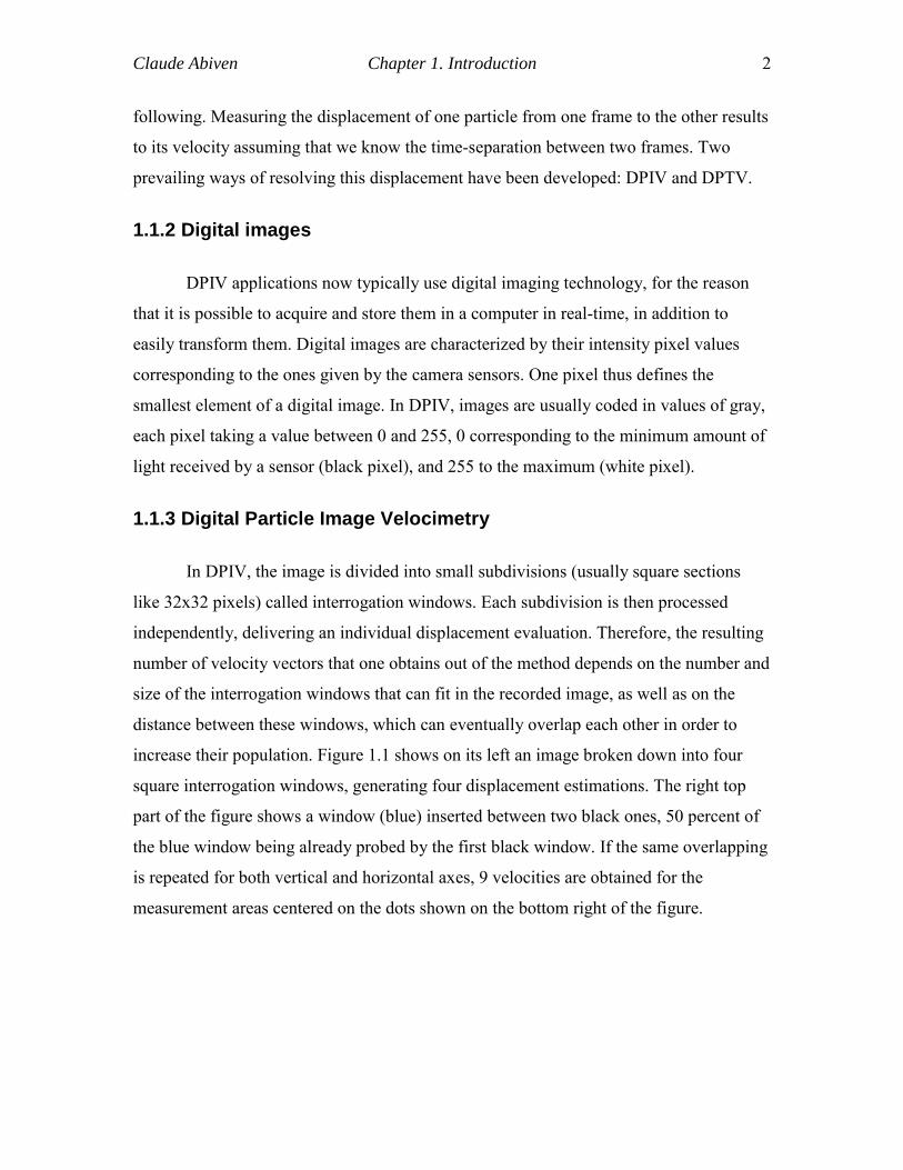
In DPIV, the image is divided into small subdivisions (usually square sections
like 32x32 pixels) called interrogation windows. Each subdivision is then processed
independently, delivering an individual displacement evaluation. Therefore, the resulting
number of velocity vectors that one obtains out of the method depends on the number and
size of the interrogation windows that can fit in the recorded image, as well as on the
distance between these windows, which can eventually overlap each other in order to
increase their population. Figure 1.1 shows on its left an image broken down into four
square interrogation windows, generating four displacement estimations. The right top
part of the figure shows a window (blue) inserted between two black ones, 50 percent of
the blue window being already probed by the first black window. If the same overlapping
is repeated for both vertical and horizontal axes, 9 velocities are obtained for the
measurement areas centered on the dots shown on the bottom right of the figure.
Claude Abiven Chapter 1. Introduction 3
Figure1.1: Interrogation windows overlapping
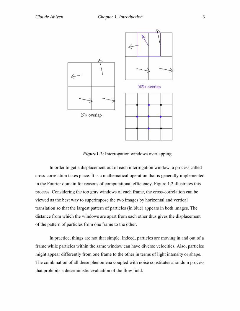
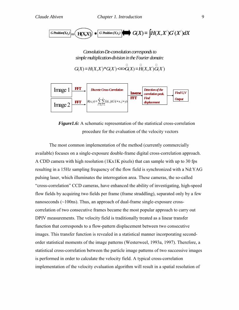
In order to get a displacement out of each interrogation window, a process called
cross-correlation takes place. It is a mathematical operation that is generally implemented
in the Fourier domain for reasons of computational efficiency. Figure 1.2 illustrates this
process. Considering the top gray windows of each frame, the cross-correlation can be
viewed as the best way to superimpose the two images by horizontal and vertical
translation so that the largest pattern of particles (in blue) appears in both images. The
distance from which the windows are apart from each other thus gives the displacement
of the pattern of particles from one frame to the other.
In practice, things are not that simple. Indeed, particles are moving in and out of a
frame while particles within the same window can have diverse velocities. Also, particles
might appear differently from one frame to the other in terms of light intensity or shape.
The combination of all these phenomena coupled with noise constitutes a random process
that prohibits a deterministic evaluation of the flow field.
Claude Abiven Chapter 1. Introduction 4
Figure1.2: Cross-correlation procedure
1.1.4 Digital Particle Tracking Velocimetry, Hybrid DPTV
DPTV stands for Digital Particle Tracking Velocimetry. It differs from DPIV in
the sense that instead of trying to find the displacements using clusters of particles, each
particle form the first frame is identified, and directly matched with the corresponding
particle in the second frame. This can be done using size, shape, brightness, or closeness
criteria for particle differentiation and identification. The corresponding displacement
then simply is the difference of position of the particle between the two frames. The
Claude Abiven Chapter 1. Introduction 5
drawback of DPTV clearly is the difficulty to distinguish one particle among the others.
On the other hand, its advantage is its ability to resolve different velocities from one
particle to another no matter how close they are to each other, while two close particles
with dissimilar velocities will not be distinguishable by the DPIV. DPIV results can be
used by the DPTV in order to facilitate the search task, in a procedure called Hybrid
DPTV.
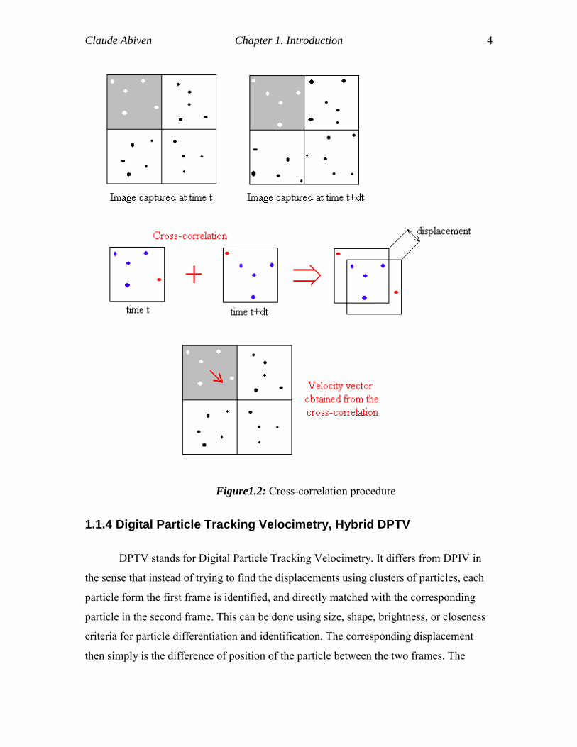
1.1.5 Typical arrangement of the experimental setup
Both DPIV and DPTV use digital images as an input. A usual experimental setup
enabling one to capture these images is presented in figure 1.3.
Figure1.3: General overview of an experimental setup
Claude Abiven Chapter 1. Introduction 6
In the present case, the object of the study was the wake of the flow behind a
cylinder. The flow was seeded with particles (usually 10 to 100 micro-meters hollow
glass spheres with a density close to the density of water). These particles were
illuminated by a thin sheet of light, created by a laser beam going through specific optics.
Images of the particles within the flow were then captured using a digital camera. Details
of the experimental parameters can be found in Vlachos et el. (1998)
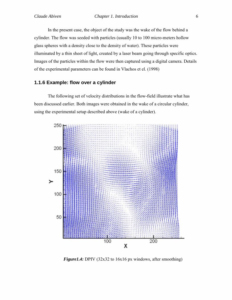
1.1.6 Example: flow over a cylinder
The following set of velocity distributions in the flow-field illustrate what has
been discussed earlier. Both images were obtained in the wake of a circular cylinder,
using the experimental setup described above (wake of a cylinder).
Figure1.4: DPIV (32x32 to 16x16 px windows, after smoothing)
Claude Abiven Chapter 1. Introduction 7
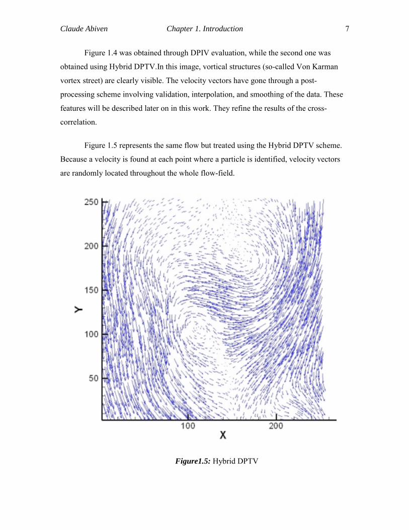
Figure 1.4 was obtained through DPIV evaluation, while the second one was
obtained using Hybrid DPTV.In this image, vortical structures (so-called Von Karman
vortex street) are clearly visible. The velocity vectors have gone through a post-
processing scheme involving validation, interpolation, and smoothing of the data. These
features will be described later on in this work. They refine the results of the cross-
correlation.
Figure 1.5 represents the same flow but treated using the Hybrid DPTV scheme.
Because a velocity is found at each point where a particle is identified, velocity vectors
are randomly located throughout the whole flow-field.
Figure1.5: Hybrid DPTV
Claude Abiven Chapter 1. Introduction 8
1.2 Previous work and objectives
1.2.1 Traditional DPIV implementation
The origin of the method goes back to traditional qualitative particle-flow
visualizations, however the early work of Meynard (1983) established the foundations of
its present form. During the past two decades, numerous publications have appeared
which present improvements on the technique as well as applications of the method to a
wide range of flows, varying from low-speed liquid and two-phase flows to supersonic
gas flows (Hasselinc, 1988; Adrian, 1991, 1996; Grant, 1994, 1997). It was the work of
Willert and Gharib (1991), Westerweel (1993a,b), and Huang and Gharib (1997) that
established the digital implementation of PIV, where the photographic film is replaced
with a CCD camera. In addition, Particle Tracking Velocimetry falls in the same general
category of particle-based techniques, which use a pulsed light source. In their basic
implementations, both methods are limited to two-dimensional velocity measurements,
but they can be extended to three dimensions (Dracos and Gruen, 1998; Hinsch and
Hinrichs, 1996; Adrian et. al., 1995; Prasad and Adrian, 1993; Adrian, 1996). PIV and
PTV are similar methods as they are both based on the same principle. The velocity is
determined from the displacement of particles within a fixed time interval. Their basic
differences are: a) in PIV, the time step is determined by the pulsing frequency of the
illumination source, while in PTV, it is determined either by the frame rate of the camera
used or by the number of pulses per frame for single-frame particle tracking; and b) most
importantly, the PTV requires low-particle concentration so that there is no overlap
between particle-image displacements (Dalziel, 1993; Perkings and Hunt, 1989). These
two considerations limit the PTV to lower flow speeds and result in a smaller density of
velocity vectors in comparison with the PIV. Furthermore, for single-frame particle
tracking, using multiple exposures per frame requires resolution of the directional
ambiguity. In contrast, conventional PIV algorithms are based on cross-correlations
performed using the FFT (as illustrated in figure 1.6), which limit the application of the
method in cases where multiple phases coexist.
Claude Abiven Chapter 1. Introduction 9
Image 1
Image 2
FFT
FFT
Discrete Cross-Correlation
),(),(),( / yjxiGjiGyxRK
Ki
L
Lj++=∑∑
−= −=
Inverse FFT
Detection of the correlation peak. Find displacement
Find U,V
Output
Image 1Image 1
Image 2Image 2
FFT
FFT
Discrete Cross-Correlation
),(),(),( / yjxiGjiGyxRK
Ki
L
Lj++=∑∑
−= −=
Inverse FFT
Detection of the correlation peak. Find displacement
Detection of the correlation peak. Find displacement
Find U,V
Output
Find U,V
Output
G/ Position (X/,t1 )G Position(X,t2 ) = *H(X,X/) ∫= dXXGXXHXG )(),()( ///G/ Position (X/,t1 )G Position(X,t2 ) = *H(X,X/) G/ Position (X/,t1 )G/ Position (X/,t1 )G Position(X,t2 ) = *H(X,X/)G Position(X,t2 )G Position(X,t2 ) = *H(X,X/)H(X,X/) ∫= dXXGXXHXG )(),()( ///
)(),()()(*),()( //// XGXXHXGXGXXHXG∧∧∧
=<≡>=
Convolution-De-convolution corresponds to simple multiplication-division in the Fourier domain:
Figure1.6: A schematic representation of the statistical cross-correlation
procedure for the evaluation of the velocity vectors
The most common implementation of the method (currently commercially
available) focuses on a single-exposure double-frame digital cross-correlation approach.
A CDD camera with high resolution (1Kx1K pixels) that can sample with up to 30 fps
resulting in a 15Hz sampling frequency of the flow field is synchronized with a Nd:YAG
pulsing laser, which illuminates the interrogation area. These cameras, the so-called
“cross-correlation” CCD cameras, have enhanced the ability of investigating, high-speed
flow fields by acquiring two fields per frame (frame straddling), separated only by a few
nanoseconds (~100ns). Thus, an approach of dual-frame single-exposure cross-
correlation of two consecutive frames became the most popular approach to carry out
DPIV measurements. The velocity field is traditionally treated as a linear transfer
function that corresponds to a flow-pattern displacement between two consecutive
images. This transfer function is revealed in a statistical manner incorporating second-
order statistical moments of the image patterns (Westerweel, 1993a, 1997). Therefore, a
statistical cross-correlation between the particle image patterns of two successive images
is performed in order to calculate the velocity field. A typical cross-correlation
implementation of the velocity evaluation algorithm will result in a spatial resolution of
Claude Abiven Chapter 1. Introduction 10
one vector every 16 pixels with an uncertainty of the velocity evaluation of the order of
0.1 pixels.
1.2.2 High Sample Rate Digital Cameras: CMOS versus CCD
The advantages of this approach can be summarized as follows. The use of YAG
lasers provides a high-energy/pulse (>100mJoules/pulse) light source with good
coherence and intensity profile. The CCD camera has a signal to noise ratio superior to
that of the standard photographic film, eliminates the intermediate digitization step, and
takes advantage of a fully computer-based data acquisition system. A photographic film,
however, still delivers unsurpassed spatial resolution and is able to cover up to three
decades of the turbulence spectrum. The most impressive results resolve a 1 m2 area with
300 microns spatial resolution (Adrian, 1996). In addition, the accuracy of the method is
greatly affected by the particle density and image size. The minimum particle-image
density needs to be about five pairs of particles per window of interrogation, while the
optimum particle-image diameter is approximately 1.5~2.5 pixels. The optimization of
the particle-image diameter and the seeding density will increase the signal to noise ratio
during the cross-correlation evaluation of the velocities (Willert and Gharib, 1991; Keane
and Adrian, 1990, 1991).
A major disadvantage of this approach is its inability to provide sufficient
frequency resolution, which is necessary to investigate high-frequency phenomena,
which might occur in turbulent flows. This is the major limitation of the DPIV systems
that are commercially available. In the system developed by the fluids group of Virginia
Tech, the difficulty of high sampling frequency is overcome. The effort was directed
towards the integration of a high-power pulsing laser with special type of optics and a
CMOS area-scan camera, capable of acquiring over 1000 frames per sec (fps). The result
is a DPIV system with a 10 KHz maximum sampling frequency.
Unfortunately, there is very limited work addressing issues arising from the use of
high-speed digital cameras (above 500 fps). These cameras are somewhat different in the
sense that the time interval between two consecutive frames and the transfer rate are
Claude Abiven Chapter 1. Introduction 11
fixed. These two parameters effectively establish the feasible frame rate. Subsequently,
the maximum possible frame rate affects the maximum velocities that can be measured.
On the other hand, the increase in the frame rate results in a significant decrease in the
exposure of the sensor, which limits the density of particles in the acquired images.
Adrian (1996, 1997) provided an analysis of different approaches to adjust the speed and
resolution of a PIV system. Multiple exposures per frame for the auto-correlation
implementation of the PIV have been studied extensively (Keane and Adrian, 1990,
1991) and a procedure for optimizing the pulse separation has been proposed (Boilot and
Prasad, 1996). One paradigm of multiple exposures per frame cross-correlation approach
was performed by Cenedese and Paglialuga (1990). However they used an analog low-
speed camera. Moreover, instead of performing a cross-correlation of the particle patterns
to determine the displacement, they initially determined the centroids of the particles and
then cross-correlated the projections of these centroids in each direction.
Conventional DPIV systems employ CCD cameras, which suffer from leakage
effects. Namely, the excessive charge from overexposed pixels leaks to the neighboring
ones saturating the whole area. In contrast, a CMOS sensor will isolate the individual
pixels behaving as a cut-off filter without leaking the energy. Therefore, by employing
CMOS technology we eliminate the blooming effect, allowing resolution of a multi-phase
flow with direct imaging within a laser sheet. This feature is of great importance since it
simplifies the experimental setup, it enhances the signal-to-noise ratio, and more
importantly could allow accurate shape and size quantification of droplets or bubbles
present in the flow. In addition, it improves the performance of the three-point centroid
gaussian estimator, as it will be explained in the paragraphs related to the hybrid particle
tracking methodology.
The quantitative flow visualization methodology that is presented in this effort is
the first to fully implement CMOS technology and take advantage of the enhanced
capabilities that it delivers.
Claude Abiven Chapter 1. Introduction 12
1.2.3 Multiphase flow
Although Digital Particle Image Velocimetry (DPIV) is the most established
global flow field measurement technique, time-resolved measurements with simultaneous
velocity, shape and size characterization of multiple phases remains a great challenge.
Major limitations stem from the fact that conventional DPIV systems employ low-frame
rate CCD cameras that are insufficient for resolving the intrinsic time-dependent flow
characteristics. Leakage effects significantly compromise the signal-to-noise ratio of the
recorded images. For multi-phase flows, saturation of the image from overexposure of
bubbles or droplets is a prohibitive parameter for carrying out accurate quantitative
measurements. Finally, high-frame-rate cameras are limited by reduced spatial resolution,
(~128x128 pixels), while the maximum measurable velocities greatly depend upon the
frame rate. These limitations are very often accounted for by employing complex
experimental setups.
Previous implementation of time-resolved systems employed digital sensors with
limited resolution (Whydrew et al ,1999) or drum cameras that are limited both in
recording times as well as frame rate (Lecordier and Trinite, 1999). Previous work by
Vlachos (2000) presented a fully digital system, which however was limited to 1KHz
sampling rate and 256x256 pixel resolution. Recent work by Upatnieks et al (2002)
presented an analog based kilohertz frame rate PIV system capable of recording up to
4000 fps with 8000 frames per sec (fps). By employing analog recording the system
delivers superior spatial resolution (>1Kx1K), however due to the fact that such high
frame rates require extreme rotation speed for the film, the registration of the images is
compromised by film alignment errors that are added on the common digitization errors.
The system presented in the scope of this work delivers a sampling frequency
between 1KHz and 10KHz, with a total acquisition time up to 4 secs and resolution
1Kx1K pixels down to 256x256 pixels.
Claude Abiven Chapter 1. Introduction 13
1.2.4 Image processing tools
Taking advantage of the unique capabilities of the imaging sensor, image pre-
processing tools were developed to allow direct phase separation within the flow.
Khalitov and Longmire (2002) presented an image-based approach for resolving two-
phase flows between a flow tracer and a solid phase. In the present work the image
processing methodologies were advanced in order to address cases where poly-dispersed
distributions of gas-bubbles, solids and/or liquids coexist in the flow. In order to develop
a flexible and versatile method capable of tackling complicated multi-phase flows, a wide
variety of image pre-processing tools were developed, such as dynamic thresholding,
Gaussian smoothing, Laplacian edge detection, filtering, erosion, multiple masking
operations and many more, as it will be explained in the chapter relative to methods and
facilities.
1.2.5 Dynamically Adaptive DPIV method
A velocity evaluation method for multiphase flows is developed, based on a
hybrid scheme that integrates a dynamically adaptive cross-correlation method with a
particle tracking velocimetry algorithm. Each phase present in the flow is processed
independently, using a multi-pass dynamically adaptive algorithm.
One of the innovations of the present work resulted from the fact that for the
analysis of polydispersed multi-phase flows, we have to account for the presence of
multiple length scales. Very often the interrogation window will contain a large-scale
droplets or bubbles, which in effect will compromise the cross-correlation resulting in
erroneous vectors. In order to preserve the advantages of the adaptive algorithm without
affecting the quality of the resulting velocity measurements, an improved adaptive cross-
correlation scheme optimized towards multi-phase flows was developed.
1.2.5.1. Dynamic windowing
In order to satisfy the Nyquist frequency criterion, a displacement has to be
smaller than one-half the length of the interrogation window in order to alleviate aliasing
Claude Abiven Chapter 1. Introduction 14
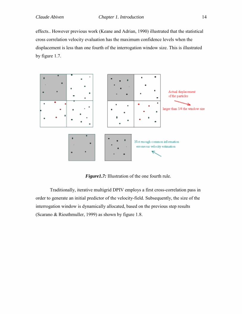
effects.. However previous work (Keane and Adrian, 1990) illustrated that the statistical
cross correlation velocity evaluation has the maximum confidence levels when the
displacement is less than one fourth of the interrogation window size. This is illustrated
by figure 1.7.
Figure1.7: Illustration of the one fourth rule.
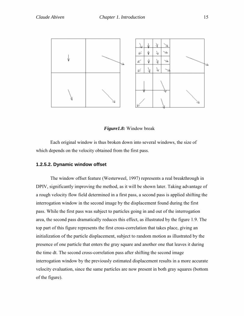
Traditionally, iterative multigrid DPIV employs a first cross-correlation pass in
order to generate an initial predictor of the velocity-field. Subsequently, the size of the
interrogation window is dynamically allocated, based on the previous step results
(Scarano & Rieuthmuller, 1999) as shown by figure 1.8.
Claude Abiven Chapter 1. Introduction 15
Figure1.8: Window break
Each original window is thus broken down into several windows, the size of
which depends on the velocity obtained from the first pass.
1.2.5.2. Dynamic window offset
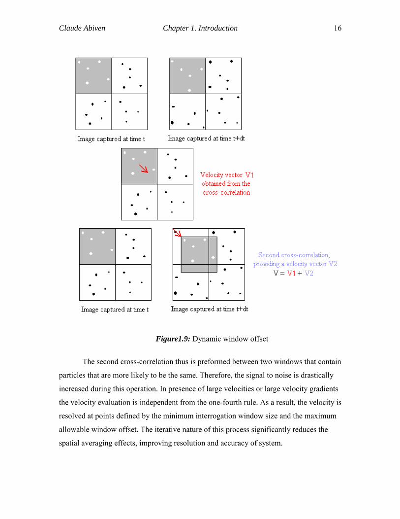
The window offset feature (Westerweel, 1997) represents a real breakthrough in
DPIV, significantly improving the method, as it will be shown later. Taking advantage of
a rough velocity flow field determined in a first pass, a second pass is applied shifting the
interrogation window in the second image by the displacement found during the first
pass. While the first pass was subject to particles going in and out of the interrogation
area, the second pass dramatically reduces this effect, as illustrated by the figure 1.9. The
top part of this figure represents the first cross-correlation that takes place, giving an
initialization of the particle displacement, subject to random motion as illustrated by the
presence of one particle that enters the gray square and another one that leaves it during
the time dt. The second cross-correlation pass after shifting the second image
interrogation window by the previously estimated displacement results in a more accurate
velocity evaluation, since the same particles are now present in both gray squares (bottom
of the figure).
Claude Abiven Chapter 1. Introduction 16
Figure1.9: Dynamic window offset
The second cross-correlation thus is preformed between two windows that contain
particles that are more likely to be the same. Therefore, the signal to noise is drastically
increased during this operation. In presence of large velocities or large velocity gradients
the velocity evaluation is independent from the one-fourth rule. As a result, the velocity is
resolved at points defined by the minimum interrogation window size and the maximum
allowable window offset. The iterative nature of this process significantly reduces the
spatial averaging effects, improving resolution and accuracy of system.
Claude Abiven Chapter 1. Introduction 17
1.2.5.3. Drawbacks of conventional implementations
Both dynamic window offset and dynamic windowing were implemented during
this effort. One of the major drawbacks of the window offset feature is that any incorrect
evaluation of the velocity during the first pass inescapably leads to erroneous velocity
estimations for any velocity vector that was computed using this velocity offset. Indeed
the steps subsequent to the first pass refine the velocity evaluation assuming that it was
originally properly evaluated. Two original approaches to overcome this problem were
developed. The first one is minimizing the effect of the erroneous offset by using a
specific offset for each sub-window, and the second is checking the validity of the offset.
1.2.6 Hybrid particle tracking method
1.2.6.1. Particle detection
Every particle detection scheme takes advantage of image processing tools. A
clean image that ensures proper particle detection significantly affects the particle
tracking performance.
Guezennec and Kiritsis (1990) proposed a method to ensure the particle detection.
It consists in examining each pixel of the image line by line. For each pixel above a
certain threshold, its eight neighbors are recursively examined. If they don’t belong to
any particle, a new particle number is assigned to the pixel. If they belong to a previously
identified particle, the current pixel is added to the list. In some cases, the neighbor pixels
belong to two different particles. In this last case, the “two” particles are actually one, and
need to be reconnected. All the pixels belonging to one of them have thus to be assigned
to the other, as well as the current pixel. This algorithm links each pixel of the image to a
particle.
In the scope of this work, this algorithm is significantly improved, accounting for
overlapping or neighboring particles that would appear as one if conventional processing
were used.
Claude Abiven Chapter 1. Introduction 18
1.2.6.2. Particle pairing
Since the work by Guezennec and Kiritsis (1990), DPTV is tightly related to
DPIV, using the results from the cross-correlation in order to initialize the hybrid
particle-tracking scheme. Indeed, based on the results from the cross-correlation,
estimating the displacement of each particle (from frame one) is straightforward, leading
to the expected position of the particle in the second frame, and considerably narrowing
the radius of search for each particle pairing. This scheme usually ensures the pairing of
most of the particles present in the flow.
An enhancement was proposed by Cowen and Monismith (1997) who suggested
to correlate a window centered on each remaining particle (in frame one) with another
one centered at the expected particle location (in frame two) before checking if the result
of this correlation would lead to a corresponding close enough particle in the second
frame.
Taking advantage of the cross-correlation methodologies developed for the DPIV,
a method similar to the one by Cowen and Monismith is proposed, avoiding any
interpolation in order to estimate the velocity of the particles, an issue common to every
DPTV scheme.
19
Chapter 2 Methods and facilities
In this chapter, the methods and facilities employed during the realization of this
work are presented. It includes the hardware components involved in the test cases, the
way artificial images are generated, a description of the image processing techniques
employed all along this effort, and an explanation of the statistical analyses used to
validate the software’s performance.
2.1 Hardware facilities
2.1.1 Hardware components
The following provides a basic description of all the basic hardware components
involved in the experimental test cases.
Copper Vapor Laser: High frequency, high-power laser: This laser was the
workhorse of the DPIV system developed in the ESM Fluid Mechanics Laboratory. This
is a copper vapor 55-Watt pulsing laser with nominal range of operation of the laser is at
10KHz. However, the repetition rate is controllable using an external signal. Previous
work performed by member of our group (Vlachos 2000) with the collaboration of the
laser manufacturing company resulted to a customization of the pulse generation
components of the laser extending the range of operation from 100 Hz to 30 KHz. Near
its operational limits, the laser experiences power loses. At a frequency of 10KHz
(nominal frequency) the power output per pulse is in the order of 5mJ. This number is
low compared with the low frequency Nd:YAG lasers that are commonly used.
Phantom IV CMOS 512Kx512K-30000 fps Digital Camera: Two of these
cameras are currently available to the Virginia Tech Fluid Mechanics Laboratory. The
second camera provides color capabilities. It is the first commercially available optical
sensor based on CMOS-technology that delivers repetition rates up to 1000 fps with full
frame and up to 30,000 fps with reduced image format. In addition, it is more sensitive
and eliminates entirely the leakage effect of conventional CCD sensors increasing the
Claude Abiven Chapter 2. Methods and facilities 20
signal to noise ratio by almost two orders of magnitude. More specifically, this camera
delivers 100,000:1 blooming ratio with no pixel-to-pixel spill over. In other words, the
saturation of the CCD sensor that results from over exposure or from illumination of
droplets or bubbles is entirely eliminated. The sensitivity of the sensor is quantified with
the following equivalent ASA rating: with 0 contrast and 0 illumination the camera
scores an amazing 800ASA. This translates to a very important feature. The increase of
the frame rate results into a significant reduction of the light allowed on the surface of the
sensor. However, this is no longer an important problem since the sensitivity of the
camera compensates for the reduced illumination as well as for the low energy output of
the Cu-Vapor laser. These unique capabilities of the camera are essential to allow PIV
measurements and droplet/bubble sizing with such high sampling frequency.
Phantom V CMOS 1Kx1K-60000 fps Digital Camera: This is the current state
of the art camera, the generation after Phantom-IV. Delivers identical imaging
capabilities as the previous version with the additional advantage that it increases the
spatial resolution by a factor of four and doubles the maximum frame rate. It also delivers
shorter exposure time, thus higher sensitivity and faster image buffer transfer rate. This
camera was on loan from the manufacturing company for a short period of time during
which it was used to carry out part of the two-phase flow experiments that serve as test
cases of the system under development.
D/A timer controllers: Two Digital/Analog Input Output boards will be used
during this project. A Computer Boards PCI-CTR05 timer counter board that provides
five independent counters with TTL signals and time resolution of 100nsec. Second, a
National Instruments multifunctional board that provides two counters, analog inputs and
outputs, and most importantly time resolution down to 50nsecs. The later is the primary
board on which the data acquisition control scheme was developed developed.
Three Image processing and data reduction workstations: high-end PC’s were
used as workstations to provide the computer processing capabilities necessary.
Claude Abiven Chapter 2. Methods and facilities 21
Camera Lenses: Four different types of lenses are available:(1) Schneider 25mm
wide-angle lens with a continuously variable f# down to 0.95. (2) Nikkon 55mm lens
with f# 1.2 (3) Nikkon 80-300mm telephoto lens with f# 2.8. (4) Nikkon 16-100mm f#
1.9.
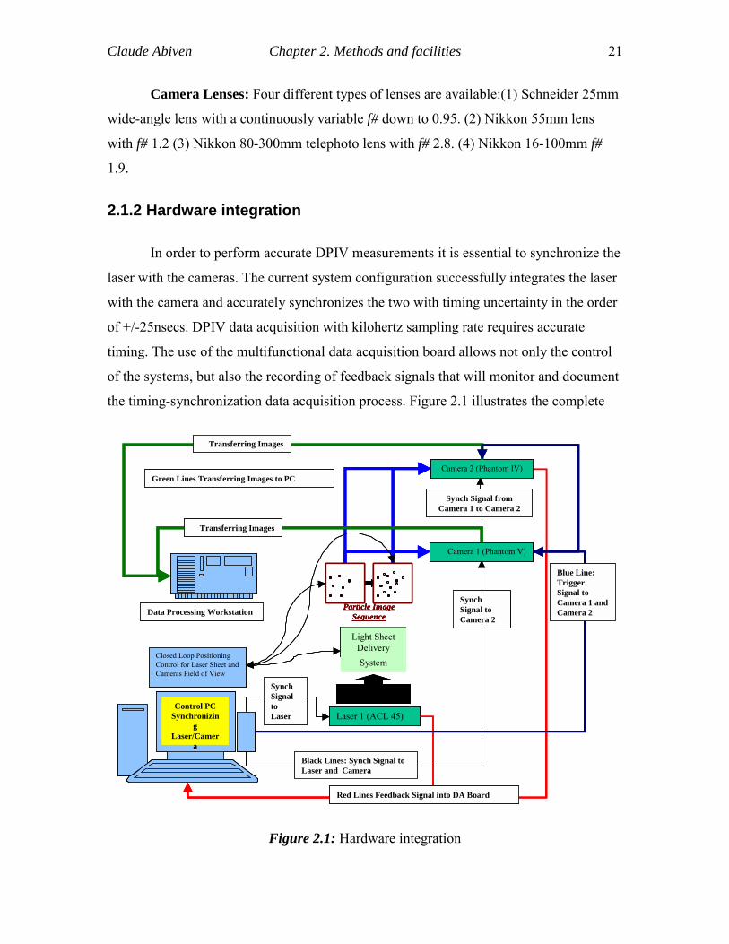
2.1.2 Hardware integration
In order to perform accurate DPIV measurements it is essential to synchronize the
laser with the cameras. The current system configuration successfully integrates the laser
with the camera and accurately synchronizes the two with timing uncertainty in the order
of +/-25nsecs. DPIV data acquisition with kilohertz sampling rate requires accurate
timing. The use of the multifunctional data acquisition board allows not only the control
of the systems, but also the recording of feedback signals that will monitor and document
the timing-synchronization data acquisition process. Figure 2.1 illustrates the complete
Light Sheet Delivery System
Laser 1 (ACL 45)
Camera 2 (Phantom IV)
Camera 1 (Phantom V)
Particle Image SequenceData Processing Workstation
Black Lines: Synch Signal to Laser and Camera
Synch Signal to Camera 2
Synch Signal from Camera 1 to Camera 2
Green Lines Transferring Images to PC
Control PCSynchronizin
g Laser/Camer
a
Transferring Images
Transferring Images
Red Lines Feedback Signal into DA Board
Synch Signal to Laser
Blue Line: Trigger Signal to Camera 1 and Camera 2
Closed Loop Positioning Control for Laser Sheet and Cameras Field of View
Light Sheet Delivery System
Light Sheet Delivery System
Laser 1 (ACL 45)Laser 1 (ACL 45)
Camera 2 (Phantom IV)Camera 2 (Phantom IV)
Camera 1 (Phantom V)Camera 1 (Phantom V)
Particle Image Sequence
Particle Image SequenceData Processing Workstation
Black Lines: Synch Signal to Laser and Camera
Synch Signal to Camera 2
Synch Signal from Camera 1 to Camera 2
Green Lines Transferring Images to PC
Control PCSynchronizin
g Laser/Camer
a
Control PCSynchronizin
g Laser/Camer
a
Transferring Images
Transferring Images
Red Lines Feedback Signal into DA Board
Synch Signal to Laser
Blue Line: Trigger Signal to Camera 1 and Camera 2
Closed Loop Positioning Control for Laser Sheet and Cameras Field of View
Closed Loop Positioning Control for Laser Sheet and Cameras Field of View
Figure 2.1: Hardware integration
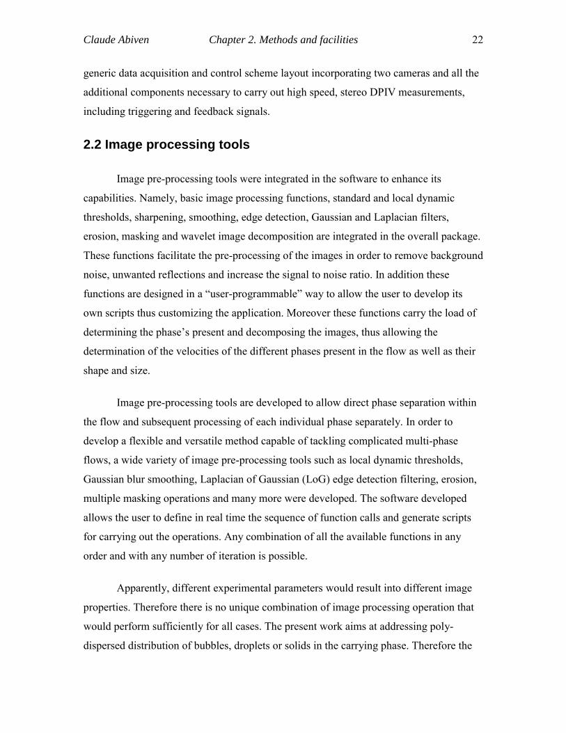
Claude Abiven Chapter 2. Methods and facilities 22
generic data acquisition and control scheme layout incorporating two cameras and all the
additional components necessary to carry out high speed, stereo DPIV measurements,
including triggering and feedback signals.
2.2 Image processing tools
Image pre-processing tools were integrated in the software to enhance its
capabilities. Namely, basic image processing functions, standard and local dynamic
thresholds, sharpening, smoothing, edge detection, Gaussian and Laplacian filters,
erosion, masking and wavelet image decomposition are integrated in the overall package.
These functions facilitate the pre-processing of the images in order to remove background
noise, unwanted reflections and increase the signal to noise ratio. In addition these
functions are designed in a “user-programmable” way to allow the user to develop its
own scripts thus customizing the application. Moreover these functions carry the load of
determining the phase’s present and decomposing the images, thus allowing the
determination of the velocities of the different phases present in the flow as well as their
shape and size.
Image pre-processing tools are developed to allow direct phase separation within
the flow and subsequent processing of each individual phase separately. In order to
develop a flexible and versatile method capable of tackling complicated multi-phase
flows, a wide variety of image pre-processing tools such as local dynamic thresholds,
Gaussian blur smoothing, Laplacian of Gaussian (LoG) edge detection filtering, erosion,
multiple masking operations and many more were developed. The software developed
allows the user to define in real time the sequence of function calls and generate scripts
for carrying out the operations. Any combination of all the available functions in any
order and with any number of iteration is possible.
Apparently, different experimental parameters would result into different image
properties. Therefore there is no unique combination of image processing operation that
would perform sufficiently for all cases. The present work aims at addressing poly-
dispersed distribution of bubbles, droplets or solids in the carrying phase. Therefore the
Claude Abiven Chapter 2. Methods and facilities 23
image-based phase separation needs to be dynamically adaptive to the temporal and
spatial changes of the recorded images. In the following paragraphs we will describe only
the most important of these operations used in one suggested processing scenario that
serves to separate the different phases and store them in individual images that will be
processed independently. It is important to note that the image processing function is
taking advantage of the capabilities of the CMOS imaging sensor in order to accurately
determine the boundaries of droplets or bubbles, as well the size and distribution of the
flow tracers.
2.2.1 Usual image processing tools
The full discussion of the image processing tools used is beyond the scope of this
work. Image processing remains a vast issue. Researchers have spent years in order to
develop and improve an arsenal of image processing strategies. The present work uses
most of them as ready to use utensils. Tools commonly used with Particle Image
Velocimetry methods developed during this effort are referenced below.
• Binarization: assign to 0 pixels under a certain pixel, and 1 to others.
• Threshold: removes every intensity pixel under a certain threshold.
• Dynamic threshold: automatically applies local thresholds to 3x3 squares
based on the pixel values inside the square.
• Erosion: removes boundaries of objects pixel layer by layer leaving single
pixels center of the object at the end of the erosion process.
• Filters3x3: modifies pixels inside a 3x3 square in terms of the 9 considered
pixel values.
• Logical and basic operations: AND, OR, addition, subtraction...
• Maximum: detects local maximums.
Claude Abiven Chapter 2. Methods and facilities 24
The aforementioned tools are very customary in image processing, and were
implemented following the methods by Jahne (Image Processing for Scientific
Applications 1991 and 1997).
A general algorithm that segregates the different phase within the flow is
presented in the following paragraphs. Although each particular case needs to be
processed specifically, the subsequent scheme can be viewed as a starting point from
which the user can add or remove image-processing operations in order to tackle each
flow’s specificity. It consists in cleaning the image using thresholds, before applying
smoothing and edge detection in order to separate the phases in the flow, and eventually
tracking the resulting particles using a particle segmentation method.
2.2.2 Thresholding
2.2.2.1. Histogram based thresholding
Background noise is a significant issue in both DPIV and DPTV. In the case of
DPIV, it mingles with the signal (particles) and contributes to inaccurate estimations of
the actual cross-correlation peak. In the case of DPTV, confusing noise and particles can
result in pairing imaginary particles, ensuing erroneous velocity estimations. Therefore, a
specific and original image-processing tool, namely histogramming, was developed
during the present effort in order to dynamically cope with background noise.
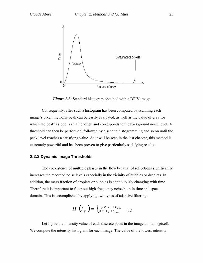
Considering images of a seeded flow-field coded in values of gray, one can plot
its histogram, that is, the number of realizations of each value of gray over the whole
image. As shown below, background noise generally appears as a peak in the low
intensity values of the histogram.
Claude Abiven Chapter 2. Methods and facilities 25
Figure 2.2: Standard histogram obtained with a DPIV image
Consequently, after such a histogram has been computed by scanning each
image’s pixel, the noise peak can be easily evaluated, as well as the value of gray for
which the peak’s slope is small enough and corresponds to the background noise level. A
threshold can then be performed, followed by a second histogramming and so on until the
peak level reaches a satisfying value. As it will be seen in the last chapter, this method is
extremely powerful and has been proven to give particularly satisfying results.
2.2.3 Dynamic Image Thresholds
The coexistence of multiple phases in the flow because of reflections significantly
increases the recorded noise levels especially in the vicinity of bubbles or droplets. In
addition, the mass fraction of droplets or bubbles is continuously changing with time.
Therefore it is important to filter out high-frequency noise both in time and space
domain. This is accomplished by applying two types of adaptive filtering.
( ) { max
max0hIifI
hIifijijij
ijIH >
<= (1.)
Let Ii,j be the intensity value of each discrete point in the image domain (pixel).
We compute the intensity histogram for each image. The value of the lowest intensity
Claude Abiven Chapter 2. Methods and facilities 26
peak (hmax) is used as a criterion. If the intensity of each pixel is higher than the
threshold value defined by the histogram, the value is preserved otherwise it is set to
zero. This operation serves to remove the low-level background noise with a threshold
value that adapts to each image. In practice, we apply this filter in an iterative manner
depending on the image noise levels. Typical value of three iterations is usually
sufficient.
2.2.4 Smoothing and Edge Detection
Area-base operations are preformed within windows of 3x3 pixels. Our objective
is to separate the dispersed phases present in the flow without altering the information of
the flow tracers. Once the low-level background noise is removed, the flow tracer
particles correspond to small wavenumber (~3pixels) high frequency elements in the
pictures. However, noise could still be present in the image, while it is important to
consider the fact that the application of gradient-based edge detector in the subsequent
step always amplifies the noise levels. Therefore, it is necessary to apply a smoothing
filter. Khalitov and Longmire (2002) proposed a classic blur filter defined as:
( )111141
+−+− +++++
= ijijjijionewo IIIIcI
cI (2.)
This effort incorporated and tested the above filter. However, our experimentation
showed that a Gaussian kernel that incorporates all the pixels in the 3x3 stencil performs
better for most cases. This filter is defined as:
+
+= ∑
∑ijijoo
ijo
newij IcIc
ccI 1 (3.)
Where Iij and cij correspond to the intensity value and the corresponding
coefficient for all the pixels within the 3x3 window except the center one which is
denoted with co and Io, where rij is the distance of each pixel in the stencil from the
center one. The center pixel coefficient can take a value of 1 for very strong smoothing
however arbitrary values can be used, depending on the images.
Claude Abiven Chapter 2. Methods and facilities 27
The Gaussian smoothing defines the first part of our LoG filter. We define a
Laplacian operator that is convolved in the two-dimensional image domain with the 3x3
pixel windows. For small wavenumbers this filter is defined as:
=1212122121
41* LwhereLI (4.)
This operation will perform as a high-pass spatial filter, practically eliminating
image elements bigger than 3x3 pixels. Subsequently we perform an area binarization,
which will set the value of the center pixel to zero or one, respectively, based on the area
information. This area binarization is defined as:
∫∫ ≥==A
IcoefdA maxsumij *9*II if 1I (5.)
An image inversion and subtraction from the original image results in recovering
the original image but with the dispersed flow elements removed. At this point we have
decomposed the original image into two. The first image contains the flow tracers, and it
will be used for performing the cross-correlation and the hybrid particle tracking velocity
field evaluation. Typically one more image-processing step is performed.
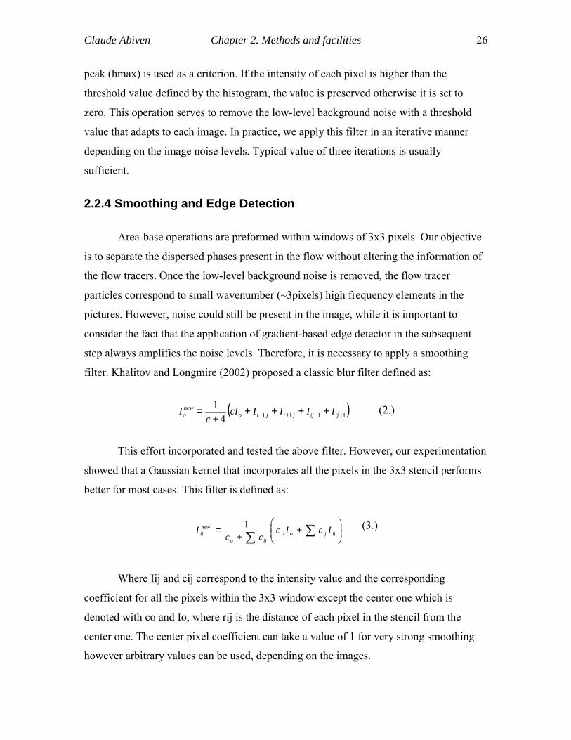
2.2.5 Particle erosion
Particle erosion is used to identify every particle using only the highest intensity
pixel. This step is extremely important during the process of particle tracking. The
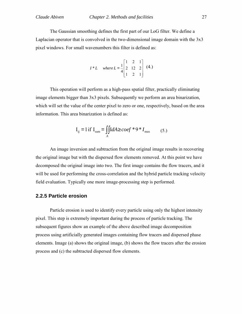
subsequent figures show an example of the above described image decomposition
process using artificially generated images containing flow tracers and dispersed phase
elements. Image (a) shows the original image, (b) shows the flow tracers after the erosion
process and (c) the subtracted dispersed flow elements.
Claude Abiven Chapter 2. Methods and facilities 28
Figure 2.3: Original image (a) before decomposition
Figure 2.4: From left to right: images (b) and (c) after decomposition
The image containing the dispersed phase can be further processed. Different
schemes can be employed to identify different size distributions. Recursive search is used
to classify pixels that are connected to each other, thus defining a single element.
Subsequently the apparent areas can be sorted with increasing size order and classified to
the different phases if more than two are present in the flow.
Claude Abiven Chapter 2. Methods and facilities 29
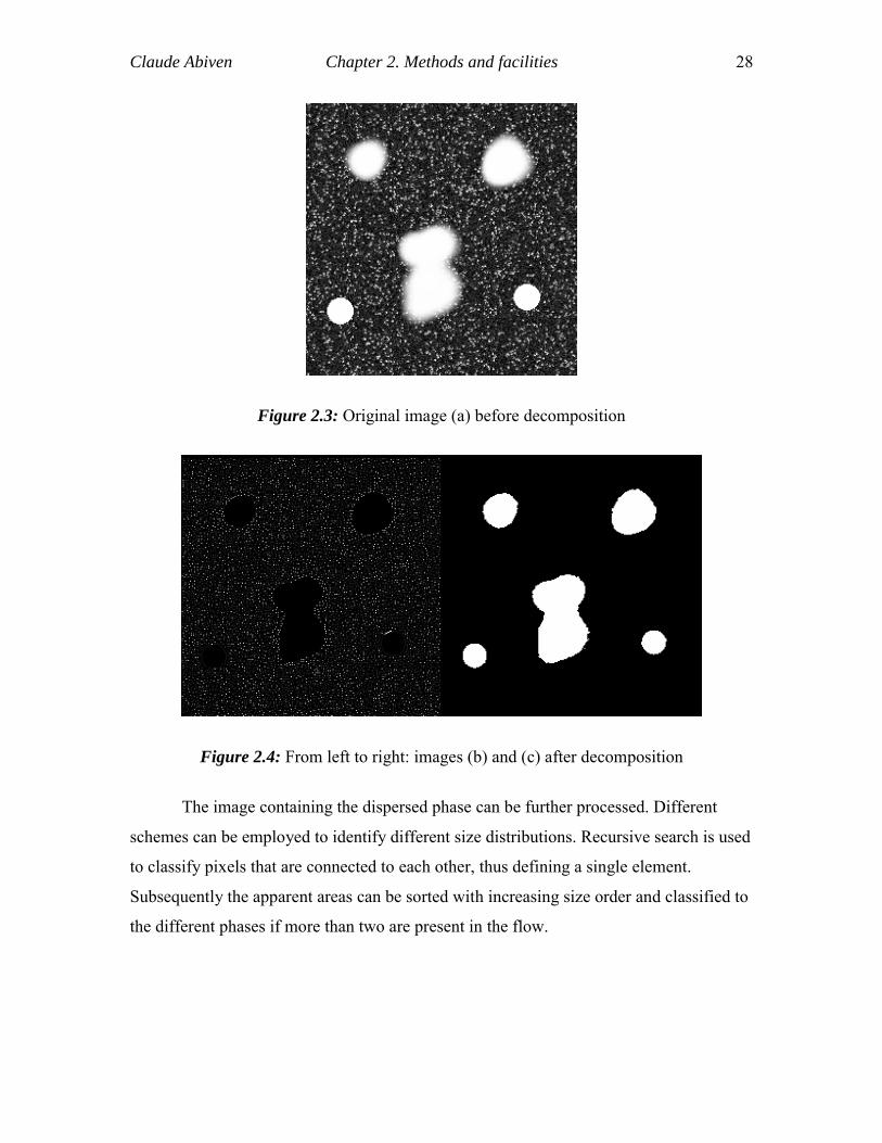
2.2.6 Big particle segmentation
These last operations can be done using the scheme by Guezennec and Kiritsis
(1990) for particle tracking velocimetry that was described earlier (paragraph 1.2.6.1.
particle detection) and that ensures particle detection. The example below (figure 2.5)
illustrates the performance of the algorithm.
Figure 2.5: Big particle segmentation
Objects of different size and shape were artificially generated within an image
with a uniform background. The scheme described above enables the detection of every
object in the picture, including its shape and size. In this example, particles with area of 5
pixels (this number was arbitrarily chosen) were automatically removed, producing the
image to the right.
2.3 Generation of artificial images
2.3.1 Purpose of the artificial images
In order to be able to quantify the accuracy of the presented system, so-called
artificial images needed to be generated. The purpose of these artificial images is to
provide a known flow-field with controlled experimental parameters such as noise,
particle diameter and displacement. Knowing the deterministic description of the flow
Claude Abiven Chapter 2. Methods and facilities 30
field (for instance a uniform displacement, a Couette flow, or a vortex), it is possible to
compare the expected value of any displacement in the flow (using the mathematical
model) with the results given by the software. It is necessary to simulate a realistic
experimental configuration, since in practice every recording of the flow field will
contain noise due to setup inaccuracy, camera limitations, etc. Therefore, by controlling
the experimental details via the generation of artificial images we can quantify the
relative weight of each parameter and perform detailed error analysis revealing the total
the bias and the random error of our measurements.
2.3.2 Particle generation, particle displacement
As shown by Adrian and Yao (1985) particle images can be approximated as
Gaussian. Therefore, a number (selected by the user) of points are randomly generated
within the image frame. Around each of these points and within a certain range, each
pixel’s intensity is evaluated based on a perfect Gaussian shape:
2
exp)( 0brIrI −= (6.)
I0 is the maximum intensity, b a coefficient related to the particle size, and r the
distance from the particle’s center. It is also possible to add artificial Gaussian noise to
the image, in order to create artificial images closer to real ones. Although several tests
were performed using noisy images all along this work, no investigation with this type of
images will be discussed here.
Once particles have been generated for the first frame, a mathematical description
of the flow field is used in order to determine the position of the particles within the
second frame. Since each particle location is known from its generation, the expected
displacement is derived based on the initial position of the particle, thus providing the
location of the particle within the second frame. For instance in the case of a vortex, the
distance from the center of the particle to the core of the vortex is computed, giving the
displacement of this particle (based on the theoretical equation of a vortex), and therefore
its new location. However, one has to be careful concerning the particles that leave the
Claude Abiven Chapter 2. Methods and facilities 31
interrogation domain between two consecutive frames: indeed, the image needs to be
reseeded in order to maintain the same number of particles from one frame to the other.
Therefore, each time a particle leaves the frame, it has to be reallocated to a new random
position where particles are supposed to appear on the frame. If we keep the example of a
vortex, the core of which is at the center of the image, particles would leave on the edges.
In the case when it wouldn’t be reseeded, or reseeded in the central part of the vortex, a
lack of particles would be noticed on the edges of the artificial images. One could also
account for this issue in seeding a larger area than needed. This would be conceivable in
the case of a vortex where every particle remains at the same distance from the center.
However, in the case of a uniform displacement for instance, no matter the original size
of the seeded area, particles would inevitably end up leaving the domain.
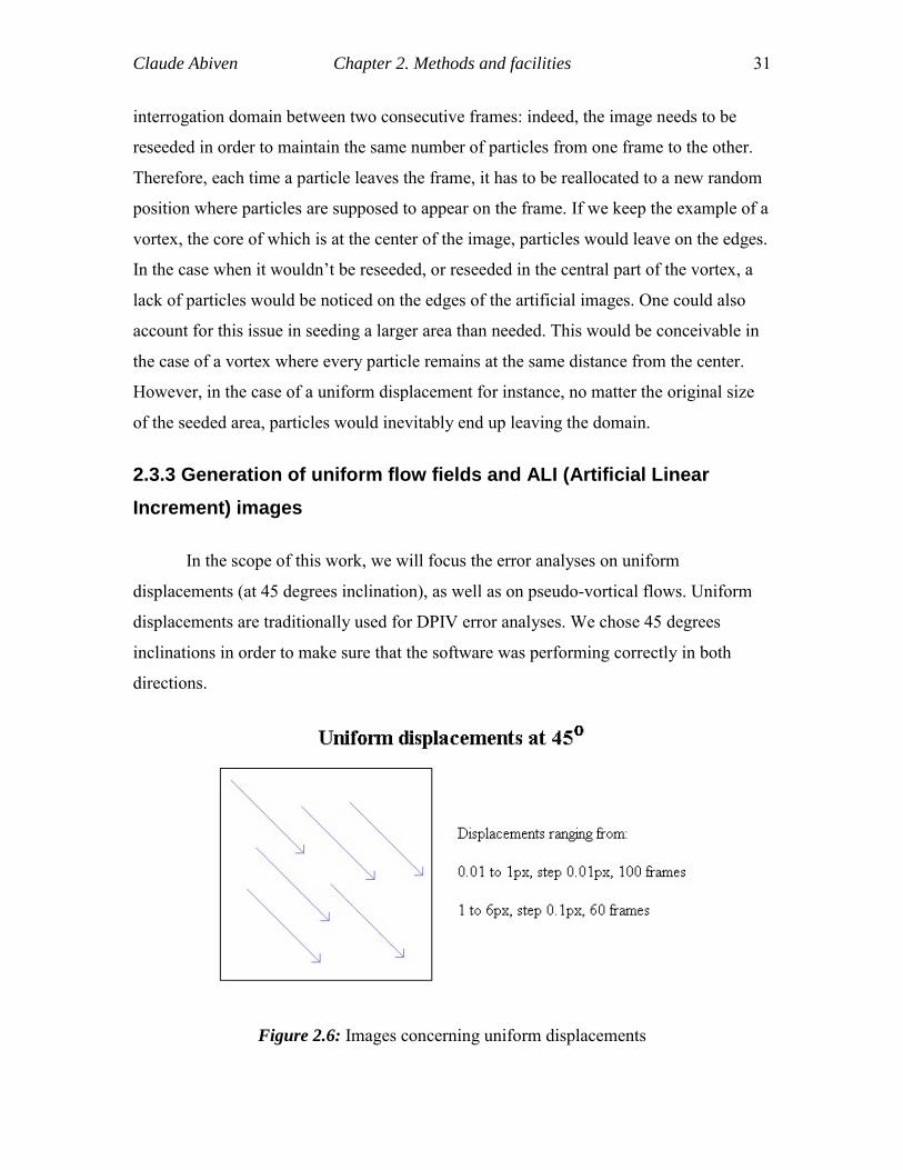
2.3.3 Generation of uniform flow fields and ALI (Artificial Linear Increment) images
In the scope of this work, we will focus the error analyses on uniform
displacements (at 45 degrees inclination), as well as on pseudo-vortical flows. Uniform
displacements are traditionally used for DPIV error analyses. We chose 45 degrees
inclinations in order to make sure that the software was performing correctly in both
directions.
Figure 2.6: Images concerning uniform displacements
Claude Abiven Chapter 2. Methods and facilities 32
Indeed, numerous features (like offsets) are implemented independently for each
axis, so that verifying the correct functioning of these features in a single direction does
not provide a full certification of the system’s performance As shown in figure 2.6,
uniform displacements were generated using 0.01 pixels steps from 0.01 pixels all the
way to 1 pixel. Also, sixty other pairs of images were generated with displacements going
from 1 to 6 pixels using steps of 0.1 pixels. Because of the discrete window offset
feature, the error pattern between zero to one pixel displacement has to be repeated with a
wave number of one pixel for all the higher displacements.
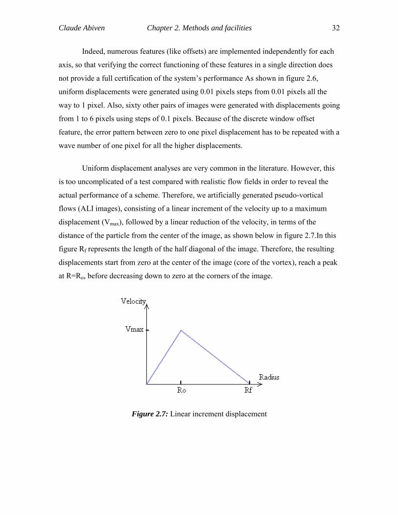
Uniform displacement analyses are very common in the literature. However, this
is too uncomplicated of a test compared with realistic flow fields in order to reveal the
actual performance of a scheme. Therefore, we artificially generated pseudo-vortical
flows (ALI images), consisting of a linear increment of the velocity up to a maximum
displacement (Vmax), followed by a linear reduction of the velocity, in terms of the
distance of the particle from the center of the image, as shown below in figure 2.7.In this
figure Rf represents the length of the half diagonal of the image. Therefore, the resulting
displacements start from zero at the center of the image (core of the vortex), reach a peak
at R=Ro, before decreasing down to zero at the corners of the image.
Figure 2.7: Linear increment displacement
Claude Abiven Chapter 2. Methods and facilities 33
−−
=⇒<<
=⇒<<
0max0
0max00
RRRR
VVRRR
RRVVRR
f
ff
(7.)
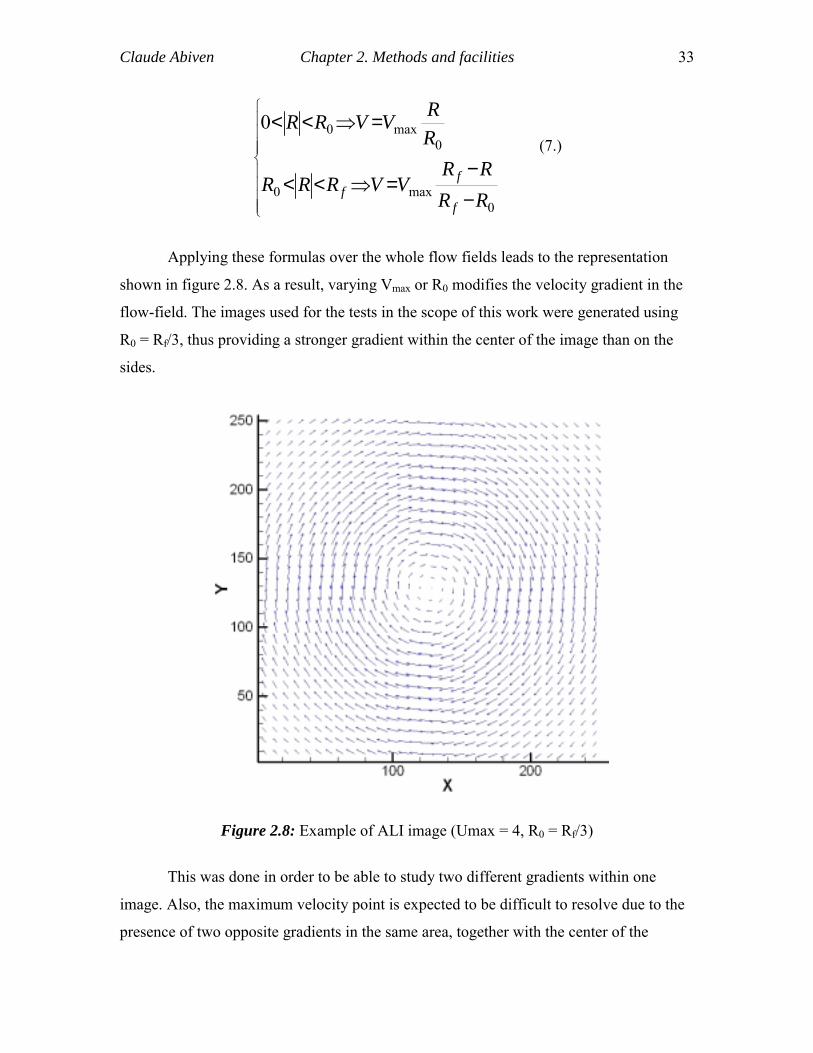
Applying these formulas over the whole flow fields leads to the representation
shown in figure 2.8. As a result, varying Vmax or R0 modifies the velocity gradient in the
flow-field. The images used for the tests in the scope of this work were generated using
R0 = Rf/3, thus providing a stronger gradient within the center of the image than on the
sides.
Figure 2.8: Example of ALI image (Umax = 4, R0 = Rf/3)
This was done in order to be able to study two different gradients within one
image. Also, the maximum velocity point is expected to be difficult to resolve due to the
presence of two opposite gradients in the same area, together with the center of the
Claude Abiven Chapter 2. Methods and facilities 34
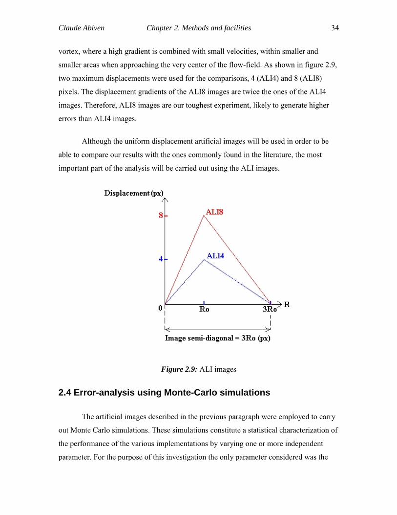
vortex, where a high gradient is combined with small velocities, within smaller and
smaller areas when approaching the very center of the flow-field. As shown in figure 2.9,
two maximum displacements were used for the comparisons, 4 (ALI4) and 8 (ALI8)
pixels. The displacement gradients of the ALI8 images are twice the ones of the ALI4
images. Therefore, ALI8 images are our toughest experiment, likely to generate higher
errors than ALI4 images.
Although the uniform displacement artificial images will be used in order to be
able to compare our results with the ones commonly found in the literature, the most
important part of the analysis will be carried out using the ALI images.
Figure 2.9: ALI images
2.4 Error-analysis using Monte-Carlo simulations
The artificial images described in the previous paragraph were employed to carry
out Monte Carlo simulations. These simulations constitute a statistical characterization of
the performance of the various implementations by varying one or more independent
parameter. For the purpose of this investigation the only parameter considered was the
Claude Abiven Chapter 2. Methods and facilities 35
displacement field. These simulations will allow us to validate our results, become aware
of mistakes inherent to the programming scheme and compare our results to previously
published ones.
Two different sets of Monte Carlo simulations were used in the scope of this
work: in the case of uniform velocities, the error was calculated in terms of the particle
displacement, whereas in the case of the ALI images, one hundred consecutive frames
depicting the same flow field were artificially generated providing an error estimation at
each point of the flow field.
2.4.1 Uniform displacements
Initially the accuracy of the method was evaluated using Monte-Carlo simulations
with artificially generated images of uniform displacement fields. In order to have a basis
for future comparisons we followed the analysis of Huang and Gharib (1997) and Huang
et al. Therefore a mean particle diameter of 2.8 pixels and particle density of 0.05
particles/pixel was selected. A Gaussian-intensity laser sheet was simulated and the
particles were uniformly distributed in all direction (x,y,z). Background white noise with
intensity of 5% was applied to simulate realistic recording conditions. The pixel
resolution was 256x256 and the vector grid spacing was 4 pixels resulting to 61x61
(3721) vectors from the cross-correlation with a minimum window of 16x16. Uniform
displacements between 0-1 pixels with displacement steps of 0.01 pixels and
displacement between 1-6 pixels with displacement step of 0.1 pixels were examined. It
is important to mention that due to the DWO application, after the first iteration, the
evaluated displacements are always between 0-0.5 pixels. The hybrid evaluation resulted
in approximately 3000 vectors for each case
For each one of the displacements under consideration, the bias, rms (root mean
square), and total error are computed over the whole flow field.
The bias error is defined as the difference between the averaged measured
velocity over the whole flow-field and the expected (known) velocity:
Claude Abiven Chapter 2. Methods and facilities 36
exp0
exp1 uuN
uuN
nnmeanbias −∑=−=
=ε (8.)
The root mean square error (the definition of which was chosen so as to be in
agreement with the publication by Huang and Gharib (1997)) is then defined as the
standard deviation of the measured velocity to its mean:
N
uuN
n meann
rms
∑
=−
= 0
2)(ε (9.)
Finally, the total error can also be computed, based on the aforementioned
definitions:
22rmsbiastotal εεε += (10.)
In the case of uniform displacements, pairs of images were artificially generated,
ranging from zero to one pixel displacement using a 0.01 pixel step (so that a hundred
pairs of images were in fact generated). Because most of PIV schemes use the window
offset (described in chapter 3), many error analyses found in the literature do not present
the error above one pixel displacement. However, programming mistakes in the
implementation of the discrete window offset or stray vectors due to noise are extremely
likely. Therefore for completeness of this analysis as well as for confirming the accurate
implementation of the various schemes it seemed particularly reasonable to incorporate in
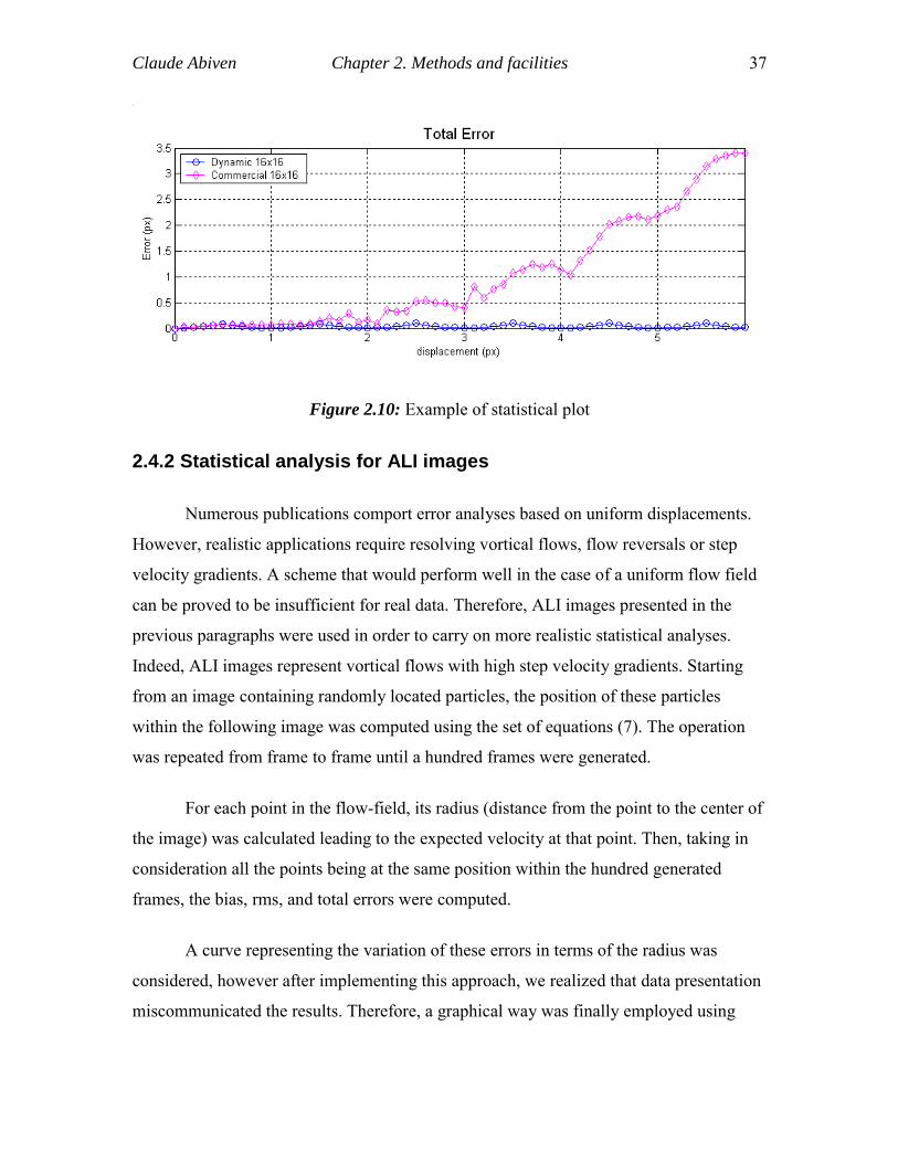
our error analysis a range from 1 to 6 pixels displacement using a 0.1 pixel step. An
example of the statistical results obtained follows in figure 2.10 (this example doesn’t
represent results discussed in this effort).
Claude Abiven Chapter 2. Methods and facilities 37
Figure 2.10: Example of statistical plot
2.4.2 Statistical analysis for ALI images
Numerous publications comport error analyses based on uniform displacements.
However, realistic applications require resolving vortical flows, flow reversals or step
velocity gradients. A scheme that would perform well in the case of a uniform flow field
can be proved to be insufficient for real data. Therefore, ALI images presented in the
previous paragraphs were used in order to carry on more realistic statistical analyses.
Indeed, ALI images represent vortical flows with high step velocity gradients. Starting
from an image containing randomly located particles, the position of these particles
within the following image was computed using the set of equations (7). The operation
was repeated from frame to frame until a hundred frames were generated.
For each point in the flow-field, its radius (distance from the point to the center of
the image) was calculated leading to the expected velocity at that point. Then, taking in
consideration all the points being at the same position within the hundred generated
frames, the bias, rms, and total errors were computed.
A curve representing the variation of these errors in terms of the radius was
considered, however after implementing this approach, we realized that data presentation
miscommunicated the results. Therefore, a graphical way was finally employed using
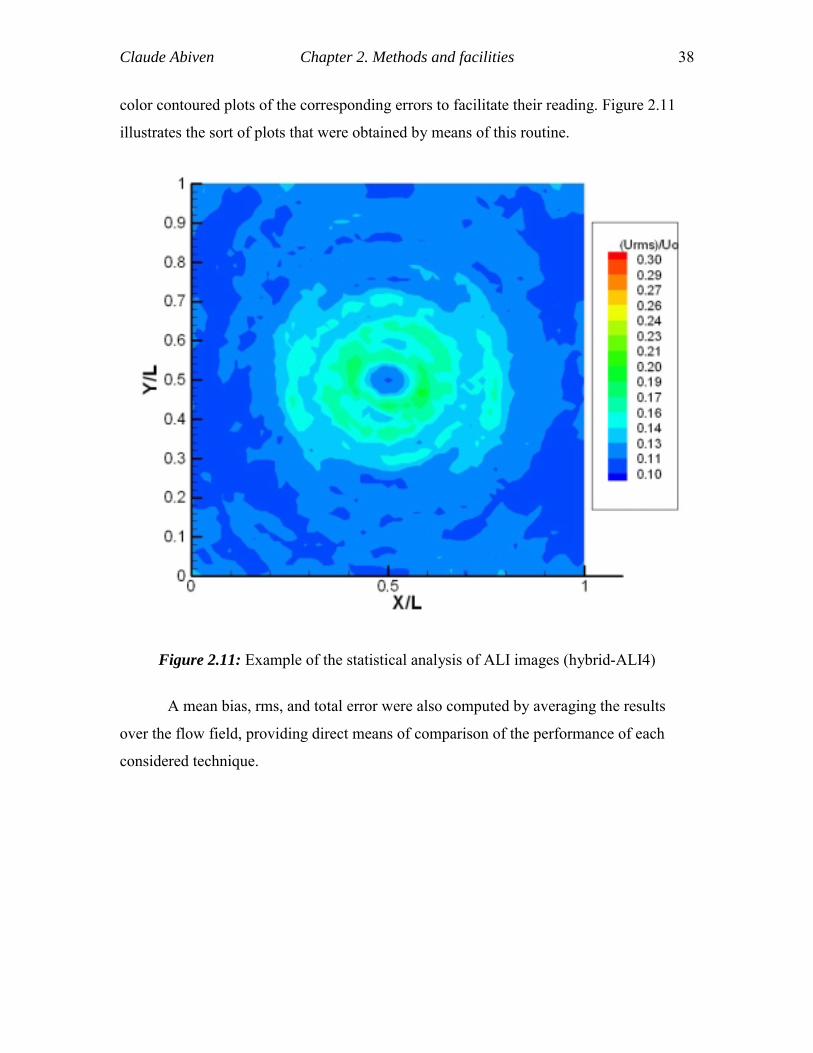
Claude Abiven Chapter 2. Methods and facilities 38
color contoured plots of the corresponding errors to facilitate their reading. Figure 2.11
illustrates the sort of plots that were obtained by means of this routine.
Figure 2.11: Example of the statistical analysis of ALI images (hybrid-ALI4)
A mean bias, rms, and total error were also computed by averaging the results
over the flow field, providing direct means of comparison of the performance of each
considered technique.
39
Chapter 3 DPIV Methods
In this chapter, we will focus on the development of the novel DPIV scheme
developed in this effort. Starting from a very basic cross-correlation, we will discuss step
by step the improvements brought to the method, as well as their effect on the accuracy
of the method. Firstly, implementations of methods presented in the literature will be
presented(dynamic adaptive window, dynamic window offset, second order offset),
followed by the original contribution of the present effort (ultimate cross-correlation and
ultimate off-check schemes).
Improvement of the cross-correlation velocity evaluation algorithms is critical for
the improvement of the performance of the system. The dynamically adaptive cross
correlation is a stand-alone module that evaluates the velocities present in the flow and
also initializes the hybrid particle-tracking scheme. Therefore, accurate estimation of
these velocities will increase the accuracy and reduce the number of stray vectors thus
minimizing the need of validation, data filtering and interpolation schemes.
3.1 Original DPIV
3.1.1 Features
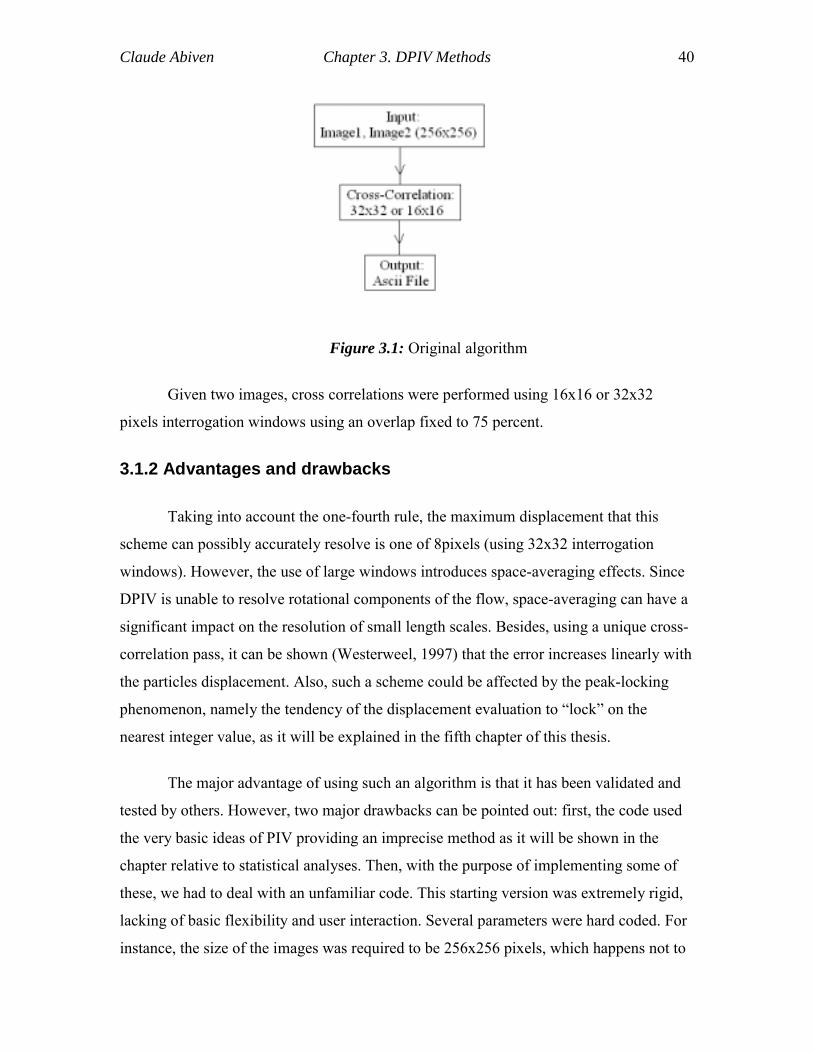
We started with the very basic algorithm by Gharib and Willert (1991). This
scheme follows the standard ideas mentioned in the first chapter of this work. Figure 3.1
gives an idea of the original algorithm that was used.
Claude Abiven Chapter 3. DPIV Methods 40
Figure 3.1: Original algorithm
Given two images, cross correlations were performed using 16x16 or 32x32
pixels interrogation windows using an overlap fixed to 75 percent.
3.1.2 Advantages and drawbacks
Taking into account the one-fourth rule, the maximum displacement that this
scheme can possibly accurately resolve is one of 8pixels (using 32x32 interrogation
windows). However, the use of large windows introduces space-averaging effects. Since
DPIV is unable to resolve rotational components of the flow, space-averaging can have a
significant impact on the resolution of small length scales. Besides, using a unique cross-
correlation pass, it can be shown (Westerweel, 1997) that the error increases linearly with
the particles displacement. Also, such a scheme could be affected by the peak-locking
phenomenon, namely the tendency of the displacement evaluation to “lock” on the
nearest integer value, as it will be explained in the fifth chapter of this thesis.
The major advantage of using such an algorithm is that it has been validated and
tested by others. However, two major drawbacks can be pointed out: first, the code used
the very basic ideas of PIV providing an imprecise method as it will be shown in the
chapter relative to statistical analyses. Then, with the purpose of implementing some of
these, we had to deal with an unfamiliar code. This starting version was extremely rigid,
lacking of basic flexibility and user interaction. Several parameters were hard coded. For
instance, the size of the images was required to be 256x256 pixels, which happens not to
Claude Abiven Chapter 3. DPIV Methods 41
be the case for many standard cameras on the market. Also, the window size was hard-
coded to 32x32 pixels. It was therefore user intensive to modify each parameter when
required. In addition no validation, interpolation, or smoothing features were
incorporated to the scheme.
Consequently, the main goal of the present effort was to improve on the basic
aforementioned version, in order to obtain a scheme subject to a reduced amount of
drawbacks.
3.1.3 Performance
3.1.3.1. Monte-Carlo simulations
Using the Monte Carlo simulations discussed in the second chapter of the present
work, we were able to quantify the error of this scheme. The error analysis presented in
figure 3.2 was carried out employing the uniform artificial images, and the DPIV scheme
used interrogation windows of 16x16 pixels. As we can see, the error is quite low for
small displacements. However, the overall error significantly increases with the
displacement. The mean total error (right of the figure, averaged form 0 to 7 pixels
displacements) is 2, which is significant. According to the one fourth rule criterion the
interrogation window size has to be at least four times the displacement of the particles
within that window while displacements up to one half of the window size are resolvable.
In this case, a 16x16 window thus should be performing correctly up to four pixels
displacement. If the bias error seems to follow that rule quite precisely, the rms error (and
consequently the overall error) begins to increase significantly for displacements larger
than two pixels.
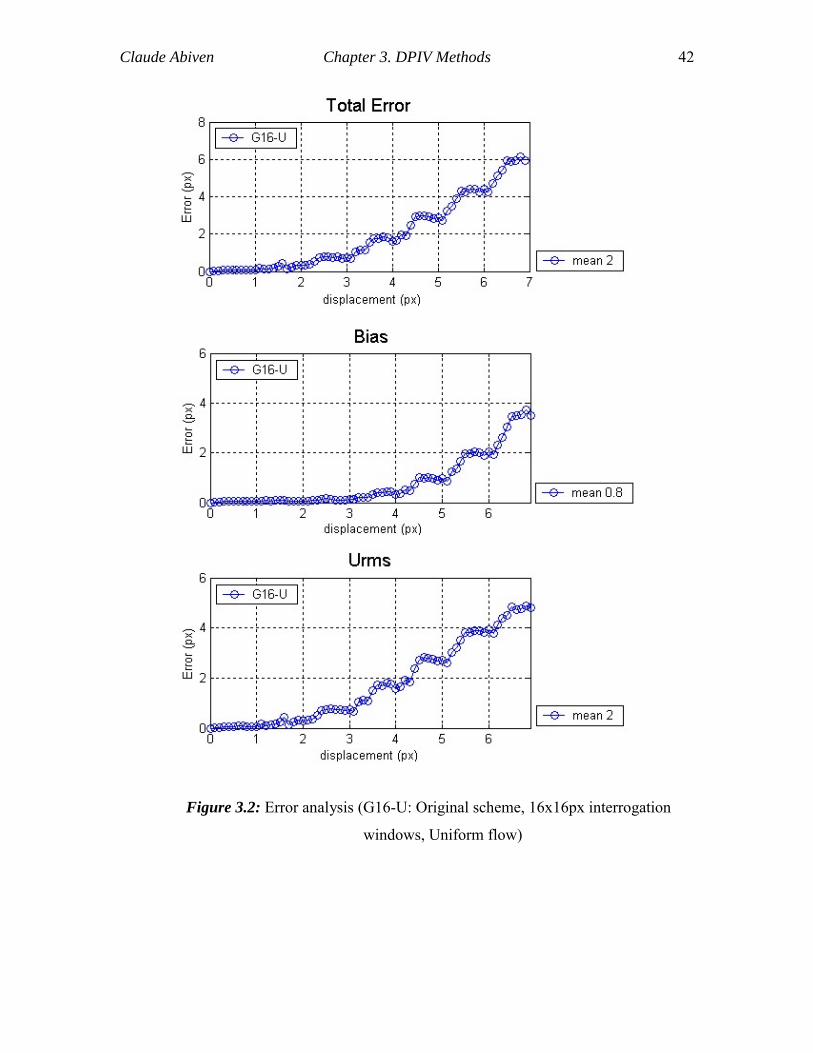
Claude Abiven Chapter 3. DPIV Methods 42
Figure 3.2: Error analysis (G16-U: Original scheme, 16x16px interrogation
windows, Uniform flow)
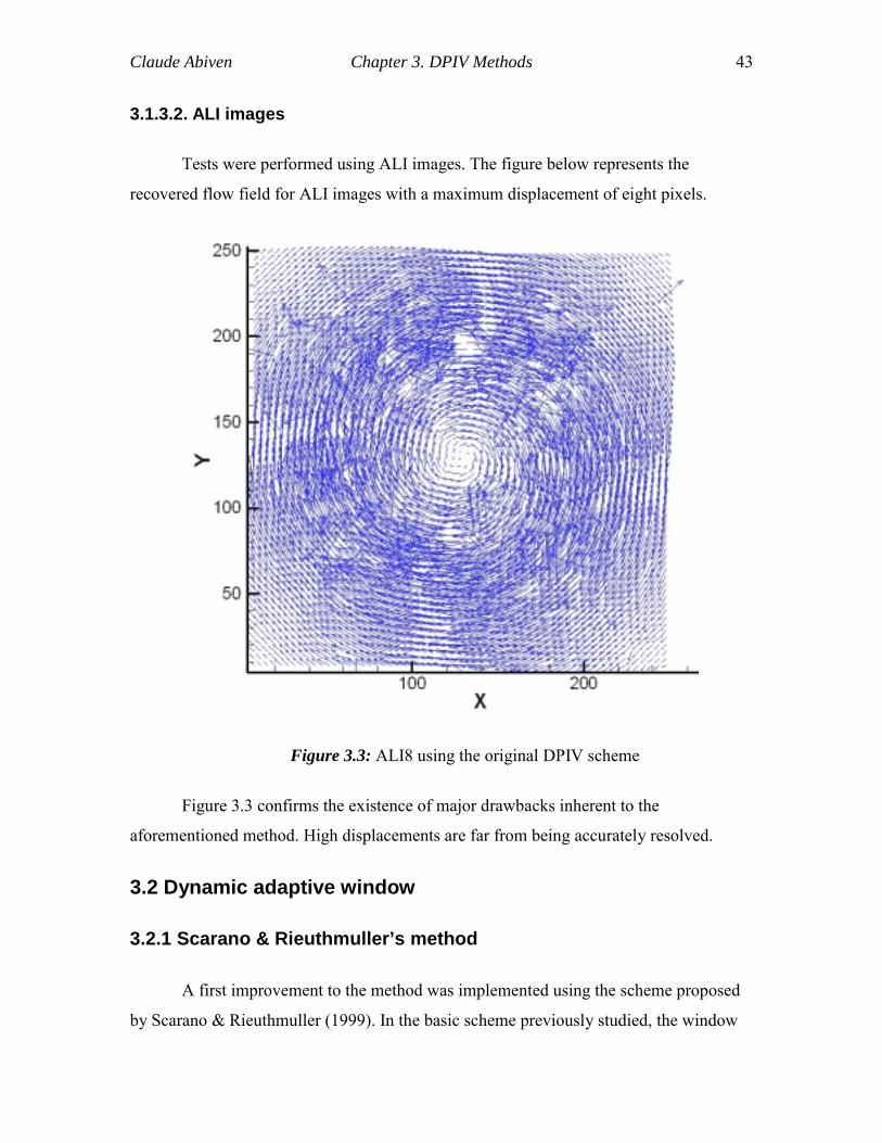
Claude Abiven Chapter 3. DPIV Methods 43
3.1.3.2. ALI images
Tests were performed using ALI images. The figure below represents the
recovered flow field for ALI images with a maximum displacement of eight pixels.
Figure 3.3: ALI8 using the original DPIV scheme
Figure 3.3 confirms the existence of major drawbacks inherent to the
aforementioned method. High displacements are far from being accurately resolved.
3.2 Dynamic adaptive window
3.2.1 Scarano & Rieuthmuller’s method
A first improvement to the method was implemented using the scheme proposed
by Scarano & Rieuthmuller (1999). In the basic scheme previously studied, the window
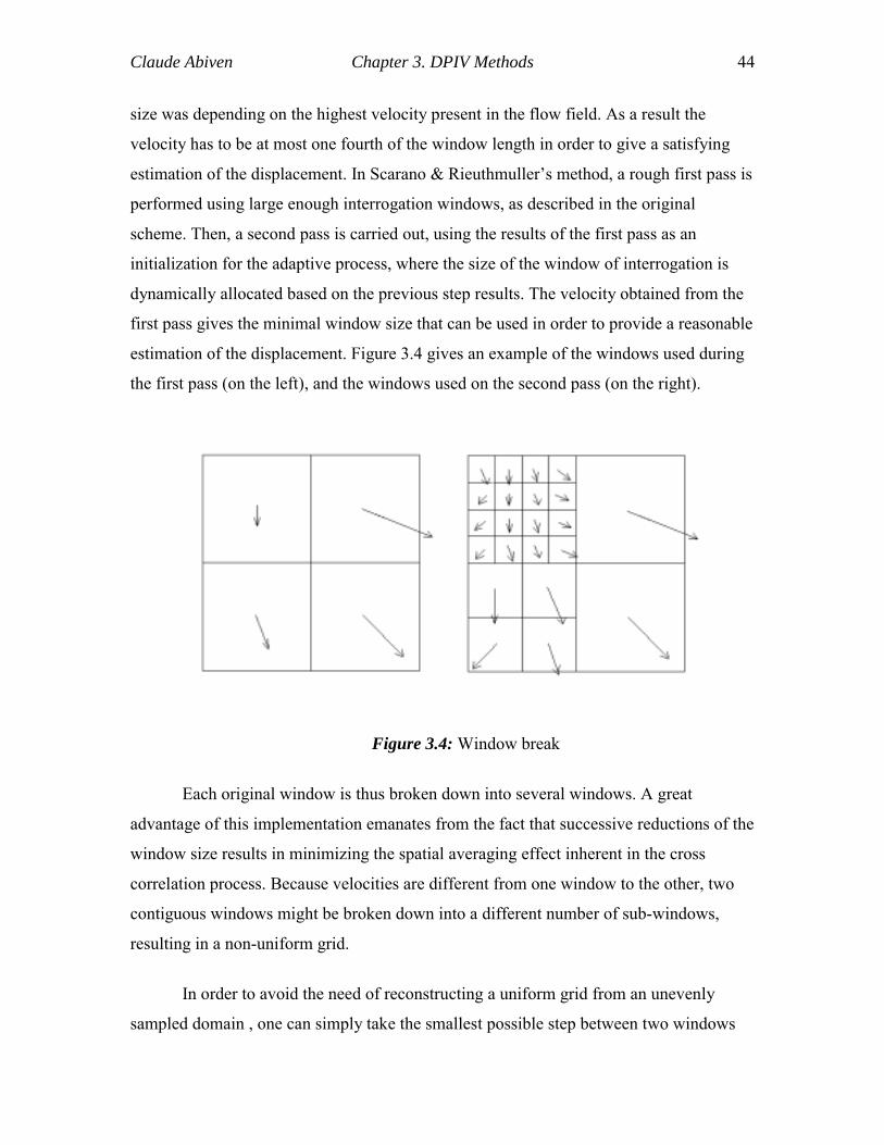
Claude Abiven Chapter 3. DPIV Methods 44
size was depending on the highest velocity present in the flow field. As a result the
velocity has to be at most one fourth of the window length in order to give a satisfying
estimation of the displacement. In Scarano & Rieuthmuller’s method, a rough first pass is
performed using large enough interrogation windows, as described in the original
scheme. Then, a second pass is carried out, using the results of the first pass as an
initialization for the adaptive process, where the size of the window of interrogation is
dynamically allocated based on the previous step results. The velocity obtained from the
first pass gives the minimal window size that can be used in order to provide a reasonable
estimation of the displacement. Figure 3.4 gives an example of the windows used during
the first pass (on the left), and the windows used on the second pass (on the right).
Figure 3.4: Window break
Each original window is thus broken down into several windows. A great
advantage of this implementation emanates from the fact that successive reductions of the
window size results in minimizing the spatial averaging effect inherent in the cross
correlation process. Because velocities are different from one window to the other, two
contiguous windows might be broken down into a different number of sub-windows,
resulting in a non-uniform grid.
In order to avoid the need of reconstructing a uniform grid from an unevenly
sampled domain , one can simply take the smallest possible step between two windows
Claude Abiven Chapter 3. DPIV Methods 45
(function of the smallest possible window size plus its overlapping) as a fixed grid, and
center a window of desired size at each point of it to perform the correlation. This simple
idea is an improvement upon Scarano & Rieuthmuller’s approach that was exploited in
this effort. Despite the obvious advantage of controlling the number of grid points
independently of the velocity field it will be demonstrated that this approach is superior
because the successive passes are initialized by displacement predictors that are evaluated
in the same measurement point as the new ones. This feature improves the performance
when vortical flows or flows with high shear are evaluated. This feature will be described
in detail in a following paragraph. Here we will focus on the basic multigrid approach.
3.2.2 Resulting improvement
Investigations were carried out using the ALI images. Figure 3.5 represents the
dynamic adaptive window performance in the case of ALI with a maximum displacement
of eight pixels.
A first pass was performed using 64x64 pixels interrogation windows, with no
overlapping, resulting in sixteen velocity vectors describing the flow field. Depending on
these velocities, windows of 32x32 down to 16x16 pixels were used during the second
pass. In the center of the image as well as on the sides, the velocities were small enough,
so that 16x16 windows could be used (blue vectors). On the right side of the center
however, the velocities found during the first pass were higher than eight pixels.
Therefore, interrogation windows of 32x32 pixels were used in that section (cyan
vectors).
During the second pass, after a displacement has been computed, its value is
compared to the window size. It is then rejected if it doesn’t satisfy the one-fourth rule,
and the result of the first pass is used instead. In figure 3.5 presented below, all the
vectors on the sides should have been blue if the displacement obtained throughout the
cross-correlation process had been found to be less than four pixels. Thus, all the red
vectors correspond to velocities the magnitude of which were found to be higher than
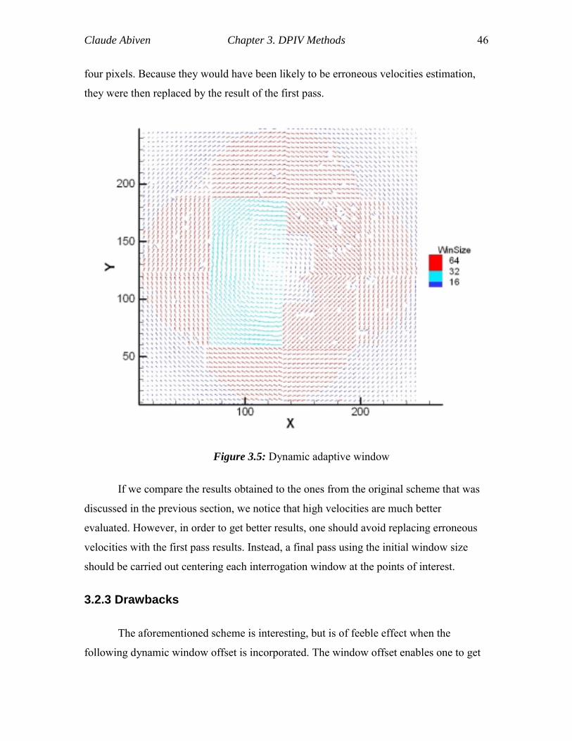
Claude Abiven Chapter 3. DPIV Methods 46
four pixels. Because they would have been likely to be erroneous velocities estimation,
they were then replaced by the result of the first pass.
Figure 3.5: Dynamic adaptive window
If we compare the results obtained to the ones from the original scheme that was
discussed in the previous section, we notice that high velocities are much better
evaluated. However, in order to get better results, one should avoid replacing erroneous
velocities with the first pass results. Instead, a final pass using the initial window size
should be carried out centering each interrogation window at the points of interest.
3.2.3 Drawbacks
The aforementioned scheme is interesting, but is of feeble effect when the
following dynamic window offset is incorporated. The window offset enables one to get
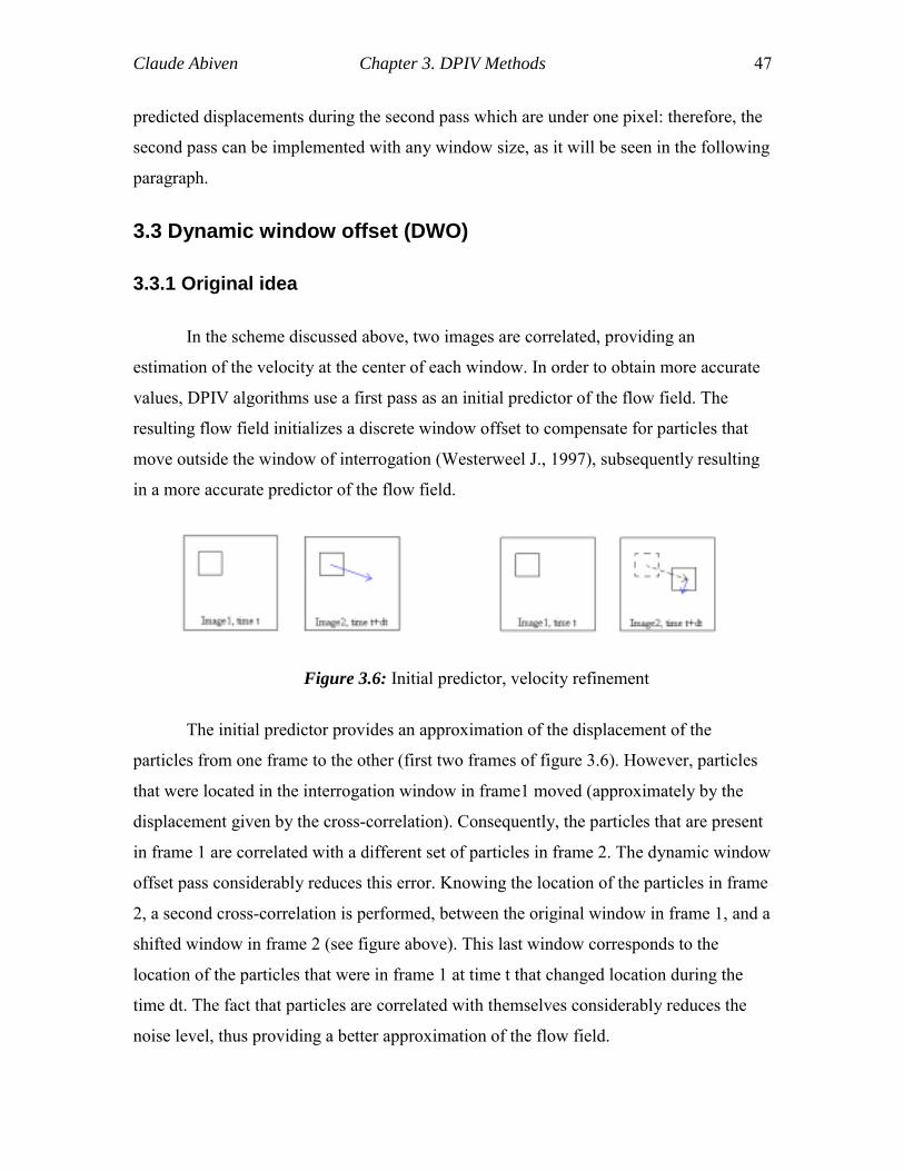
Claude Abiven Chapter 3. DPIV Methods 47
predicted displacements during the second pass which are under one pixel: therefore, the
second pass can be implemented with any window size, as it will be seen in the following
paragraph.
3.3 Dynamic window offset (DWO)
3.3.1 Original idea
In the scheme discussed above, two images are correlated, providing an
estimation of the velocity at the center of each window. In order to obtain more accurate
values, DPIV algorithms use a first pass as an initial predictor of the flow field. The
resulting flow field initializes a discrete window offset to compensate for particles that
move outside the window of interrogation (Westerweel J., 1997), subsequently resulting
in a more accurate predictor of the flow field.
Figure 3.6: Initial predictor, velocity refinement
The initial predictor provides an approximation of the displacement of the
particles from one frame to the other (first two frames of figure 3.6). However, particles
that were located in the interrogation window in frame1 moved (approximately by the
displacement given by the cross-correlation). Consequently, the particles that are present
in frame 1 are correlated with a different set of particles in frame 2. The dynamic window
offset pass considerably reduces this error. Knowing the location of the particles in frame
2, a second cross-correlation is performed, between the original window in frame 1, and a
shifted window in frame 2 (see figure above). This last window corresponds to the
location of the particles that were in frame 1 at time t that changed location during the
time dt. The fact that particles are correlated with themselves considerably reduces the
noise level, thus providing a better approximation of the flow field.
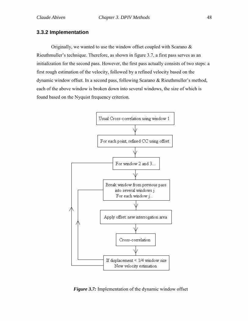
Claude Abiven Chapter 3. DPIV Methods 48
3.3.2 Implementation
Originally, we wanted to use the window offset coupled with Scarano &
Rieuthmuller’s technique. Therefore, as shown in figure 3.7, a first pass serves as an
initialization for the second pass. However, the first pass actually consists of two steps: a
first rough estimation of the velocity, followed by a refined velocity based on the
dynamic window offset. In a second pass, following Scarano & Rieuthmuller’s method,
each of the above window is broken down into several windows, the size of which is
found based on the Nyquist frequency criterion.
Figure 3.7: Implementation of the dynamic window offset
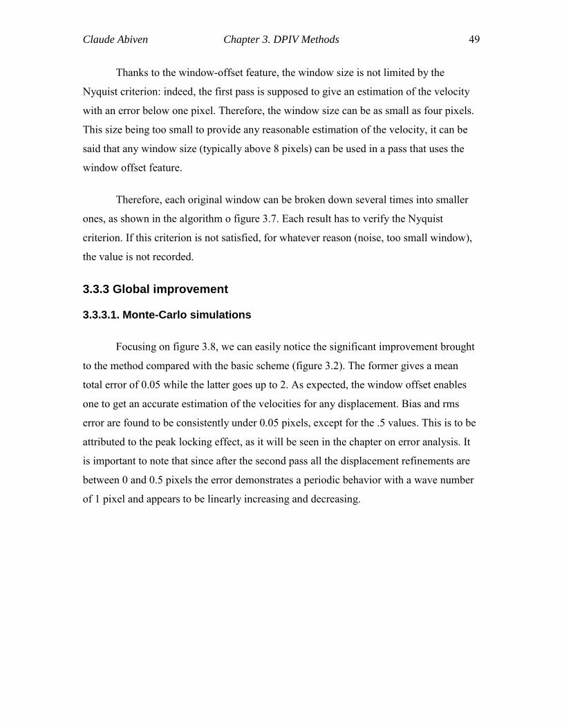
Claude Abiven Chapter 3. DPIV Methods 49
Thanks to the window-offset feature, the window size is not limited by the
Nyquist criterion: indeed, the first pass is supposed to give an estimation of the velocity
with an error below one pixel. Therefore, the window size can be as small as four pixels.
This size being too small to provide any reasonable estimation of the velocity, it can be
said that any window size (typically above 8 pixels) can be used in a pass that uses the
window offset feature.
Therefore, each original window can be broken down several times into smaller
ones, as shown in the algorithm o figure 3.7. Each result has to verify the Nyquist
criterion. If this criterion is not satisfied, for whatever reason (noise, too small window),
the value is not recorded.
3.3.3 Global improvement
3.3.3.1. Monte-Carlo simulations
Focusing on figure 3.8, we can easily notice the significant improvement brought
to the method compared with the basic scheme (figure 3.2). The former gives a mean
total error of 0.05 while the latter goes up to 2. As expected, the window offset enables
one to get an accurate estimation of the velocities for any displacement. Bias and rms
error are found to be consistently under 0.05 pixels, except for the .5 values. This is to be
attributed to the peak locking effect, as it will be seen in the chapter on error analysis. It
is important to note that since after the second pass all the displacement refinements are
between 0 and 0.5 pixels the error demonstrates a periodic behavior with a wave number
of 1 pixel and appears to be linearly increasing and decreasing.
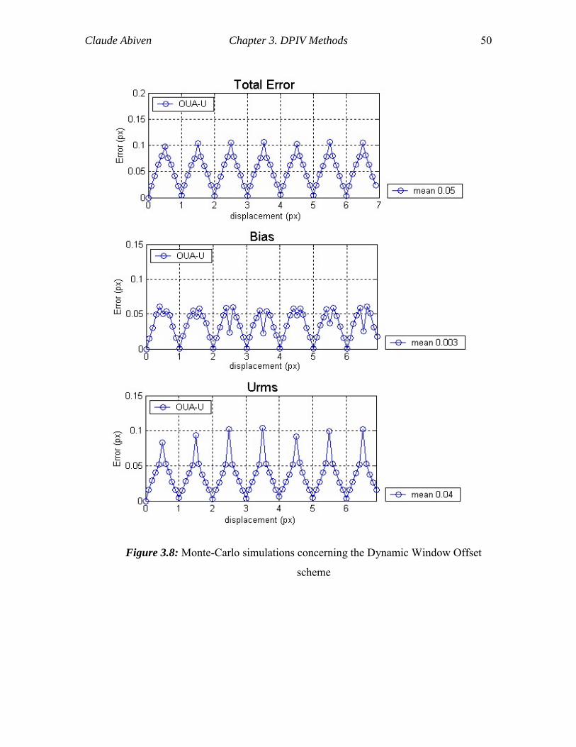
Claude Abiven Chapter 3. DPIV Methods 50
Figure 3.8: Monte-Carlo simulations concerning the Dynamic Window Offset
scheme
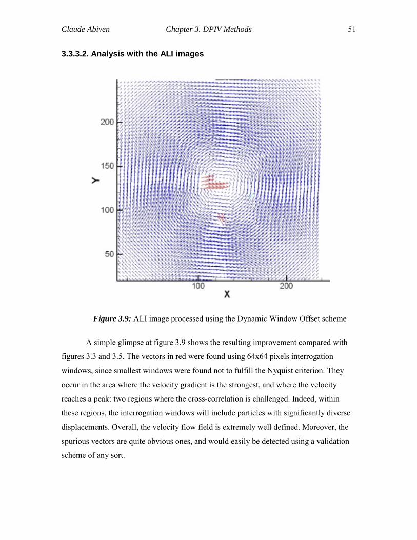
Claude Abiven Chapter 3. DPIV Methods 51
3.3.3.2. Analysis with the ALI images
Figure 3.9: ALI image processed using the Dynamic Window Offset scheme
A simple glimpse at figure 3.9 shows the resulting improvement compared with
figures 3.3 and 3.5. The vectors in red were found using 64x64 pixels interrogation
windows, since smallest windows were found not to fulfill the Nyquist criterion. They
occur in the area where the velocity gradient is the strongest, and where the velocity
reaches a peak: two regions where the cross-correlation is challenged. Indeed, within
these regions, the interrogation windows will include particles with significantly diverse
displacements. Overall, the velocity flow field is extremely well defined. Moreover, the
spurious vectors are quite obvious ones, and would easily be detected using a validation
scheme of any sort.
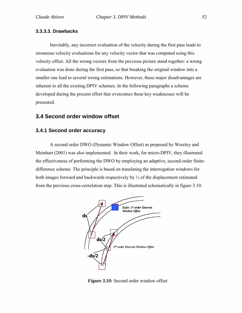
Claude Abiven Chapter 3. DPIV Methods 52
3.3.3.3. Drawbacks
Inevitably, any incorrect evaluation of the velocity during the first pass leads to
erroneous velocity evaluations for any velocity vector that was computed using this
velocity offset. All the wrong vectors from the previous picture stand together: a wrong
evaluation was done during the first pass, so that breaking the original window into a
smaller one lead to several wrong estimations. However, these major disadvantages are
inherent to all the existing DPIV schemes. In the following paragraphs a scheme
developed during the present effort that overcomes these key weaknesses will be
presented.
3.4 Second order window offset
3.4.1 Second order accuracy
A second order DWO (Dynamic Window Offset) as proposed by Wereley and
Meinhart (2001) was also implemented. In their work, for micro-DPIV, they illustrated
the effectiveness of performing the DWO by employing an adaptive, second-order finite-
difference scheme. The principle is based on translating the interrogation windows for
both images forward and backwards respectively by ½ of the displacement estimated
from the previous cross-correlation step. This is illustrated schematically in figure 3.10.
2nd order Discrete Window Offset
Euler: 1st order Discrete Window Offset
ds
-ds/2
ds/22nd order Discrete Window Offset
Euler: 1st order Discrete Window Offset
ds
-ds/2
ds/2
Euler: 1st order Discrete Window Offset
ds
-ds/2
ds/2
Figure 3.10: Second order window offset
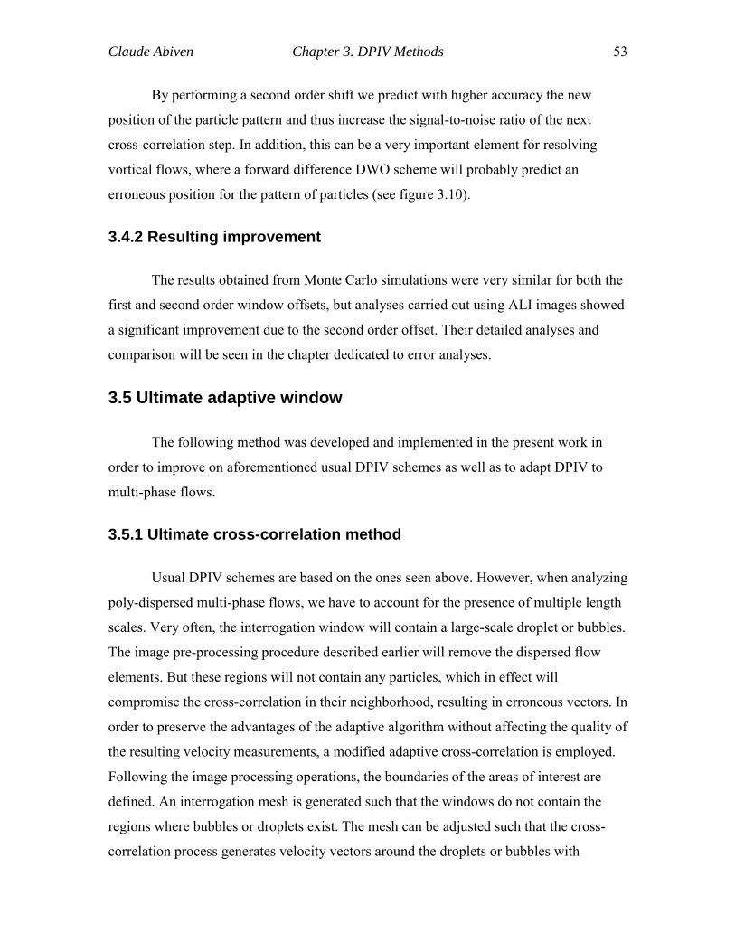
Claude Abiven Chapter 3. DPIV Methods 53
By performing a second order shift we predict with higher accuracy the new
position of the particle pattern and thus increase the signal-to-noise ratio of the next
cross-correlation step. In addition, this can be a very important element for resolving
vortical flows, where a forward difference DWO scheme will probably predict an
erroneous position for the pattern of particles (see figure 3.10).
3.4.2 Resulting improvement
The results obtained from Monte Carlo simulations were very similar for both the
first and second order window offsets, but analyses carried out using ALI images showed
a significant improvement due to the second order offset. Their detailed analyses and
comparison will be seen in the chapter dedicated to error analyses.
3.5 Ultimate adaptive window
The following method was developed and implemented in the present work in
order to improve on aforementioned usual DPIV schemes as well as to adapt DPIV to
multi-phase flows.
3.5.1 Ultimate cross-correlation method
Usual DPIV schemes are based on the ones seen above. However, when analyzing
poly-dispersed multi-phase flows, we have to account for the presence of multiple length
scales. Very often, the interrogation window will contain a large-scale droplet or bubbles.
The image pre-processing procedure described earlier will remove the dispersed flow
elements. But these regions will not contain any particles, which in effect will
compromise the cross-correlation in their neighborhood, resulting in erroneous vectors. In
order to preserve the advantages of the adaptive algorithm without affecting the quality of
the resulting velocity measurements, a modified adaptive cross-correlation is employed.
Following the image processing operations, the boundaries of the areas of interest are
defined. An interrogation mesh is generated such that the windows do not contain the
regions where bubbles or droplets exist. The mesh can be adjusted such that the cross-
correlation process generates velocity vectors around the droplets or bubbles with
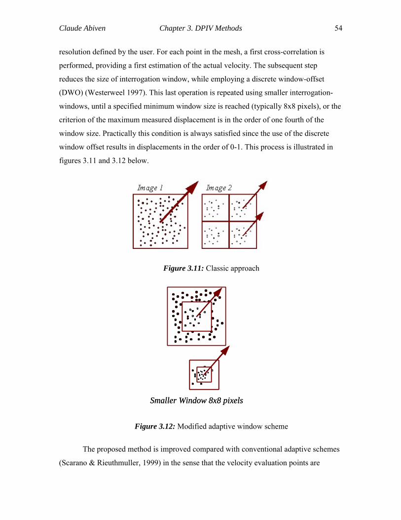
Claude Abiven Chapter 3. DPIV Methods 54
resolution defined by the user. For each point in the mesh, a first cross-correlation is
performed, providing a first estimation of the actual velocity. The subsequent step
reduces the size of interrogation window, while employing a discrete window-offset
(DWO) (Westerweel 1997). This last operation is repeated using smaller interrogation-
windows, until a specified minimum window size is reached (typically 8x8 pixels), or the
criterion of the maximum measured displacement is in the order of one fourth of the
window size. Practically this condition is always satisfied since the use of the discrete
window offset results in displacements in the order of 0-1. This process is illustrated in
figures 3.11 and 3.12 below.
Figure 3.11: Classic approach
Smaller Window 8x8 pixelsSmaller Window 8x8 pixels
Figure 3.12: Modified adaptive window scheme
The proposed method is improved compared with conventional adaptive schemes
(Scarano & Rieuthmuller, 1999) in the sense that the velocity evaluation points are
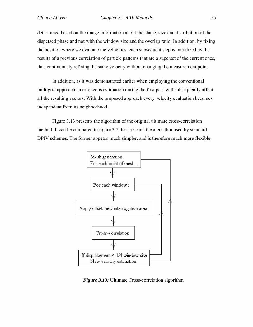
Claude Abiven Chapter 3. DPIV Methods 55
determined based on the image information about the shape, size and distribution of the
dispersed phase and not with the window size and the overlap ratio. In addition, by fixing
the position where we evaluate the velocities, each subsequent step is initialized by the
results of a previous correlation of particle patterns that are a superset of the current ones,
thus continuously refining the same velocity without changing the measurement point.
In addition, as it was demonstrated earlier when employing the conventional
multigrid approach an erroneous estimation during the first pass will subsequently affect
all the resulting vectors. With the proposed approach every velocity evaluation becomes
independent from its neighborhood.
Figure 3.13 presents the algorithm of the original ultimate cross-correlation
method. It can be compared to figure 3.7 that presents the algorithm used by standard
DPIV schemes. The former appears much simpler, and is therefore much more flexible.
Figure 3.13: Ultimate Cross-correlation algorithm
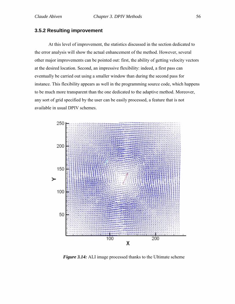
Claude Abiven Chapter 3. DPIV Methods 56
3.5.2 Resulting improvement
At this level of improvement, the statistics discussed in the section dedicated to
the error analysis will show the actual enhancement of the method. However, several
other major improvements can be pointed out: first, the ability of getting velocity vectors
at the desired location. Second, an impressive flexibility: indeed, a first pass can
eventually be carried out using a smaller window than during the second pass for
instance. This flexibility appears as well in the programming source code, which happens
to be much more transparent than the one dedicated to the adaptive method. Moreover,
any sort of grid specified by the user can be easily processed, a feature that is not
available in usual DPIV schemes.
Figure 3.14: ALI image processed thanks to the Ultimate scheme
Claude Abiven Chapter 3. DPIV Methods 57
Processing the same images as before gives only a single spurious vector (see
figure below). This improvement is likely to be due to the fact that the velocity estimation
takes place at the exact same location during each step of the process, providing a more
accurate velocity offset than usual DPIV systems. But also, a wrong velocity estimation
doesn’t lead to several wrong vectors, as in common DPIV schemes: it leads only to one,
as it can be seen in figure 3.14.
3.6 Ultimate scheme with automatic offset verification
Taking advantage of the outstanding flexibility of the ultimate method another
method -the implementation of which was hence fairly straightforward- was developed,
providing an automatic validation of the offsets as well as an automatic choice for the
window size. In other words, this method detects the specific window size that is to be
used in order to obtain the best possible estimation of the offset at each point of the flow-
field. Also, the user is informed if no realistic value could be found, preventing flow-
fields to be overrun with erroneous vectors.
3.6.1 Automatic offset verification
The weakness of the offset scheme is obviously that in the case when the offset
estimation is incorrect (this can happen when an inadequate window size is used), the
chances of recovery are slight. Therefore, detecting whether an offset has been correctly
evaluated or not could result in an immense improvement of the method. How can this be
achieved? Theoretically, the offset feature is supposed to provide a first estimation of the
particles displacement with an error smaller than one pixel. Therefore, the cross-
correlation that is performed right after the offset evaluation must give a velocity
evaluation within one half pixel. Consequently, if this requirement is not fulfilled, we can
assume that either the window size used for the offset evaluation was incorrect, or that
cross-correlation cannot be performed at the location for reasons such as a lack of
particles or a major level of noise.
As a result such observations lead one to the following line of attack: at each
location of the previously generated mesh a first pass is carried out using the first window
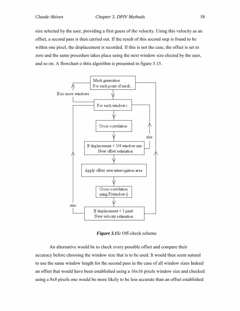
Claude Abiven Chapter 3. DPIV Methods 58
size selected by the user, providing a first guess of the velocity. Using this velocity as an
offset, a second pass is then carried out. If the result of this second step is found to be
within one pixel, the displacement is recorded. If this is not the case, the offset is set to
zero and the same procedure takes place using the next window size elected by the user,
and so on. A flowchart o thtis algorithm is presented in figure 3.15.
Figure 3.15: Off-check scheme
An alternative would be to check every possible offset and compare their
accuracy before choosing the window size that is to be used. It would then seem natural
to use the same window length for the second pass in the case of all window sizes Indeed
an offset that would have been established using a 16x16 pixels window size and checked
using a 8x8 pixels one would be more likely to be less accurate than an offset established
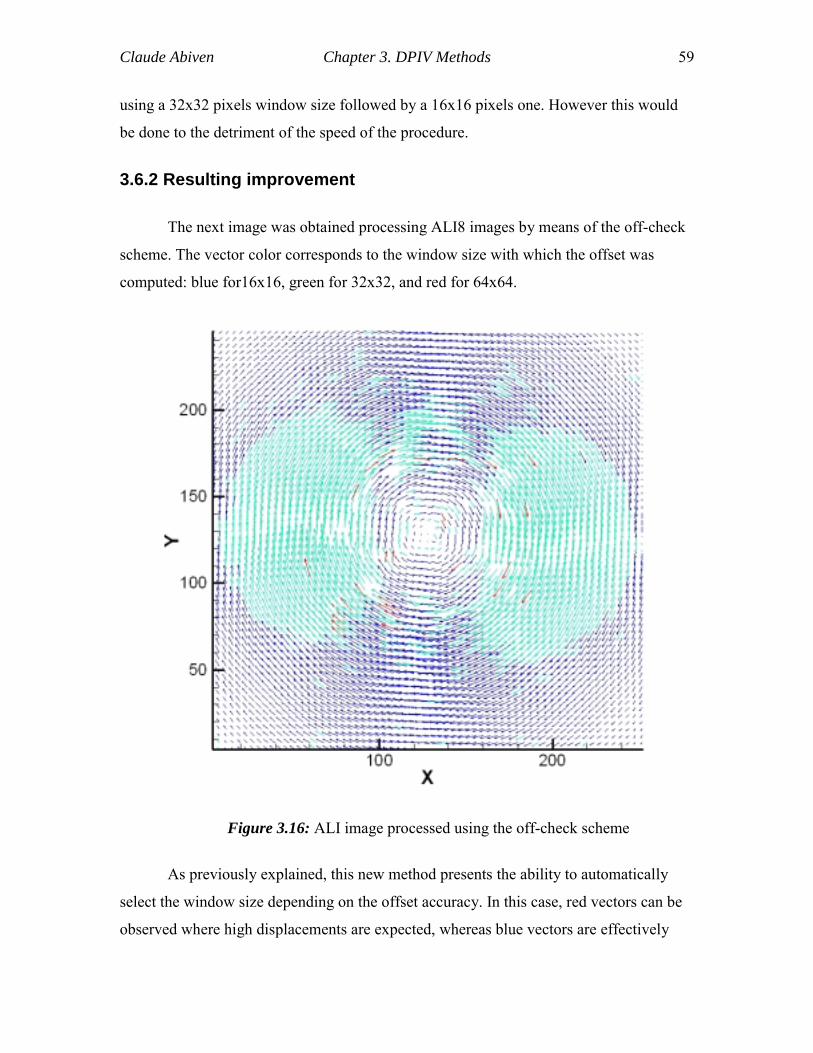
Claude Abiven Chapter 3. DPIV Methods 59
using a 32x32 pixels window size followed by a 16x16 pixels one. However this would
be done to the detriment of the speed of the procedure.
3.6.2 Resulting improvement
The next image was obtained processing ALI8 images by means of the off-check
scheme. The vector color corresponds to the window size with which the offset was
computed: blue for16x16, green for 32x32, and red for 64x64.
Figure 3.16: ALI image processed using the off-check scheme
As previously explained, this new method presents the ability to automatically
select the window size depending on the offset accuracy. In this case, red vectors can be
observed where high displacements are expected, whereas blue vectors are effectively
Claude Abiven Chapter 3. DPIV Methods 60
located where smaller displacements are expected. This method shows a remarkable
ability to remove spurious vectors, and is therefore independent of the offset-based error,
unlike usual DPIV schemes. Around 2.5 percents of the vectors were removed
(corresponding to locations for which no reasonable offset value could be computed), and
would need to be interpolated. However, further experimentations need to be carried on
before the method uncovers its full potential.
3.7 Validation
Because of noise due to particles moving in and out of plane, to the optics and
camera limitations to name a few sources of error, the cross-correlation can result in
vectors that do not correspond to the actual flow field. In order to remove these erroneous
vectors, a so-called validation scheme is usually applied as a post processor. Two
methods were studied in the present effort: a simple straightforward dynamic mean value
operator and a more advanced system based on artificial neural networks. Comparisons
between the two different methods were carried out and are presented after the
description of each scheme.
3.7.1 Dynamic mean value operator
3.7.1.1. Principle
This method is based on the work by Adrian and Meinhart (1995). It consists of
selecting eight nearest neighbors around each vector to be validated. The vector is
rejected if the difference between its magnitude and the average magnitude over its
neighbors is above a certain threshold εthres. The magnitude can be replaced by the u and
v components of the vectors, thus validating the vector direction.
For N=8 neighbors (when applicable), the following expressions are calculated:
∑
==Α
N
nnU
Nji
1)(1),(
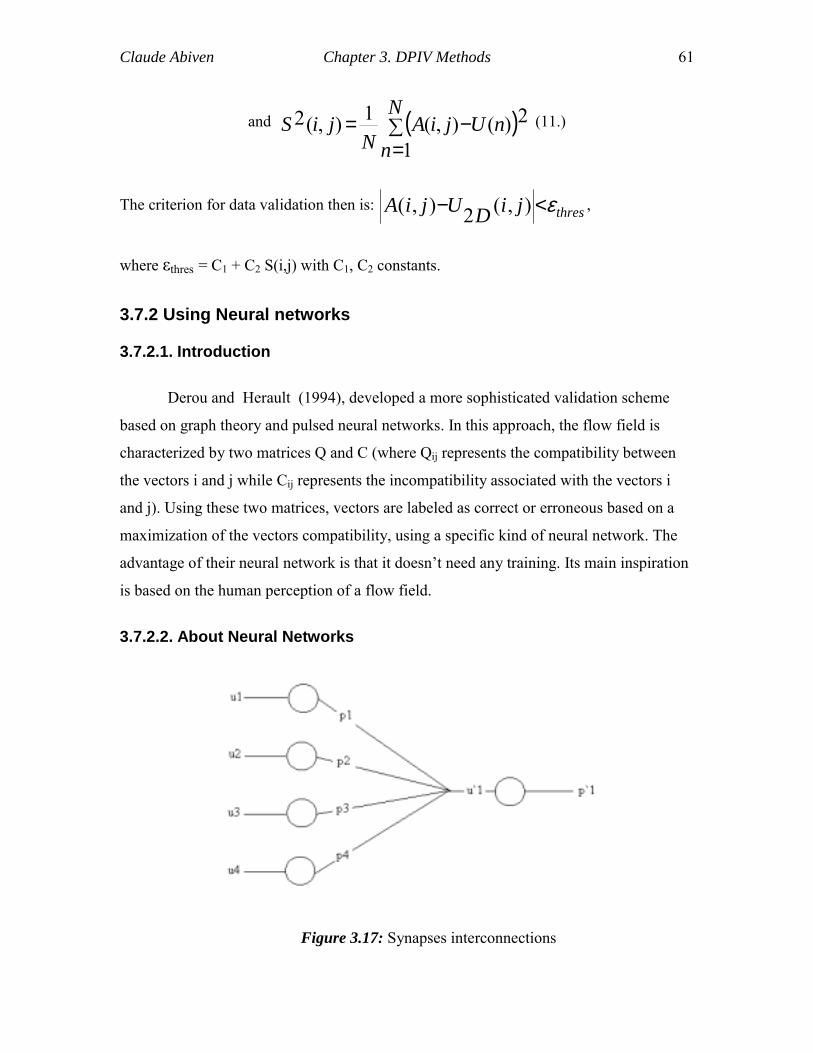
Claude Abiven Chapter 3. DPIV Methods 61
and ( )∑
=−=
N
nnUjiA
NjiS
1
2)(),(1),(2 (11.)
The criterion for data validation then is: thresjiDUjiA ε<− ),(2),( ,
where εthres = C1 + C2 S(i,j) with C1, C2 constants.
3.7.2 Using Neural networks
3.7.2.1. Introduction
Derou and Herault (1994), developed a more sophisticated validation scheme
based on graph theory and pulsed neural networks. In this approach, the flow field is
characterized by two matrices Q and C (where Qij represents the compatibility between
the vectors i and j while Cij represents the incompatibility associated with the vectors i
and j). Using these two matrices, vectors are labeled as correct or erroneous based on a
maximization of the vectors compatibility, using a specific kind of neural network. The
advantage of their neural network is that it doesn’t need any training. Its main inspiration
is based on the human perception of a flow field.
3.7.2.2. About Neural Networks
Figure 3.17: Synapses interconnections
Claude Abiven Chapter 3. DPIV Methods 62
The basic principle of the neural networks is shown below: It consists in multi-
input nodes with weighted interconnections, as indicated. If ui is the input and pi the
output of a neuron i, we can define a function H:
<>
== +
+
++
otherwisepuifuif
uHp
i
z
i
z
i
z
i
z
iβα
)1(
)1(
)1()1( 01
)( (12.)
Parameters α and β are thresholds that describe the ability of a neuron to modify
its output. If pi = 0, the neuron is deactivated, otherwise, it is activated. In the pulsed
neural network, the input of a neuron is a function of the output of the other neurons:
ui(z+1) = ui
(z) + Fi(p1(z+1), …, pN
(z+1)) (13.)
3.7.2.3. The matrices
Two matrices are created. Each coefficient mij of the n2 matrix represents a
comparison between vectors i and j.
The first matrix, Q
If the pair of vectors i and j contribute to the perception of the global movement,
of the fluid elements that correspond to their respective positions there should be able to
define a coefficient qij which will have high values; this coefficient is a function of three
additional coefficients corresponding to: similarity, good continuation, and proximity.
The similarity coefficient:
It compares the lengths of the two vectors li, lj, and their angle, as indicated by
figure 3.18.
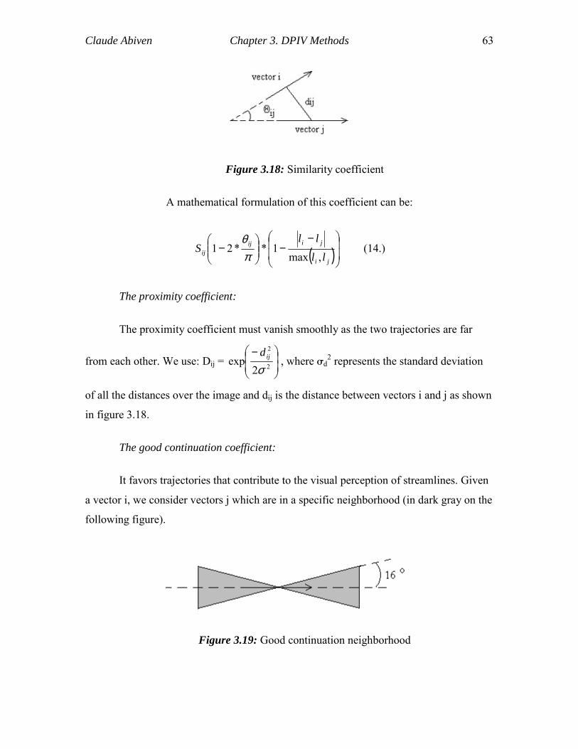
Claude Abiven Chapter 3. DPIV Methods 63
Figure 3.18: Similarity coefficient
A mathematical formulation of this coefficient can be:
( )
−−
−
ji
jiijij ll
llS
,max1**21
πθ
(14.)
The proximity coefficient:
The proximity coefficient must vanish smoothly as the two trajectories are far
from each other. We use: Dij =
−2
2
2exp
σijd
, where σd2 represents the standard deviation
of all the distances over the image and dij is the distance between vectors i and j as shown
in figure 3.18.
The good continuation coefficient:
It favors trajectories that contribute to the visual perception of streamlines. Given
a vector i, we consider vectors j which are in a specific neighborhood (in dark gray on the
following figure).
Figure 3.19: Good continuation neighborhood
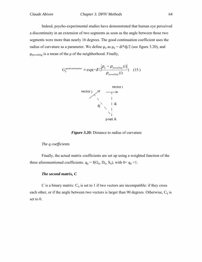
Claude Abiven Chapter 3. DPIV Methods 64
Indeed, psycho-experimental studies have demonstrated that human eye perceived
a discontinuity in an extension of two segments as soon as the angle between those two
segments were more than nearly 16 degrees. The good continuation coefficient uses the
radius of curvature as a parameter. We define ρij as ρij = di*dj/2 (see figure 3.20), and
ρprevailing is a mean of the ρ of the neighborhood. Finally,
))(
)(exp(
ii
Gprevailing
prevailingijuationgoodcontinij ρ
ρρδ
−⋅−= (15.)
Figure 3.20: Distance to radius of curvature
The q coefficients
Finally, the actual matrix coefficients are set up using a weighted function of the
three aforementioned coefficients. qij = f(Gij, Dij, Sij), with 0< qij <1.
The second matrix, C
C is a binary matrix: Cij is set to 1 if two vectors are incompatible: if they cross
each other, or if the angle between two vectors is larger than 90 degrees. Otherwise, Cij is
set to 0.
Claude Abiven Chapter 3. DPIV Methods 65
3.7.2.4. Formulation of the problem
In order to eliminate the bad vectors, let’s consider the following problem:
Let’s p = (p1, …,pN) be a vector, in which pi = 1 if the trajectory i is labeled as a
good one, and 0 otherwise. We have to find p maximizing E(p):
[ ]
=⇒==∀∈∀
∑ ∑== =
01,,,1,0,
)(1 1
ijjii
N
i
N
jjiij
Cppjipi
ppqpE (16.)
This general case can be solved using a neural network following the standard
scheme described above. In our case, the neuron i represents directly the vector i.
Therefore, if this neuron is deactivated (i.e. pi =0), the corresponding vector is considered
as erroneous. The function F mentioned earlier is chosen to respect the following
conditions: a deactivated neuron can be activated only if its new state contributes towards
an increase of the quality function E(p), and all the neurons incompatible with this one
must be deactivated. The neural network synapses, after several iterations, converge to a
maximum for E(p). This binary output corresponds directly to the vectors, labeled as
validated or erroneous.
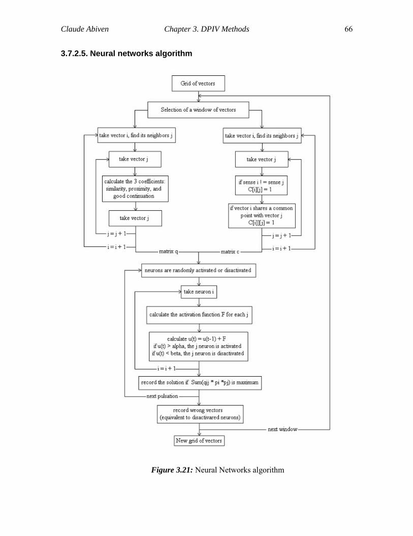
Claude Abiven Chapter 3. DPIV Methods 66
3.7.2.5. Neural networks algorithm
Figure 3.21: Neural Networks algorithm
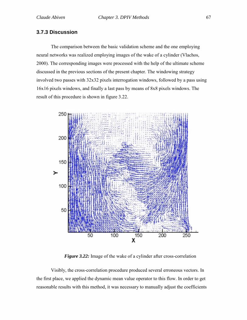
Claude Abiven Chapter 3. DPIV Methods 67
3.7.3 Discussion
The comparison between the basic validation scheme and the one employing
neural networks was realized employing images of the wake of a cylinder (Vlachos,
2000). The corresponding images were processed with the help of the ultimate scheme
discussed in the previous sections of the present chapter. The windowing strategy
involved two passes with 32x32 pixels interrogation windows, followed by a pass using
16x16 pixels windows, and finally a last pass by means of 8x8 pixels windows. The
result of this procedure is shown in figure 3.22.
Figure 3.22: Image of the wake of a cylinder after cross-correlation
Visibly, the cross-correlation procedure produced several erroneous vectors. In
the first place, we applied the dynamic mean value operator to this flow. In order to get
reasonable results with this method, it was necessary to manually adjust the coefficients
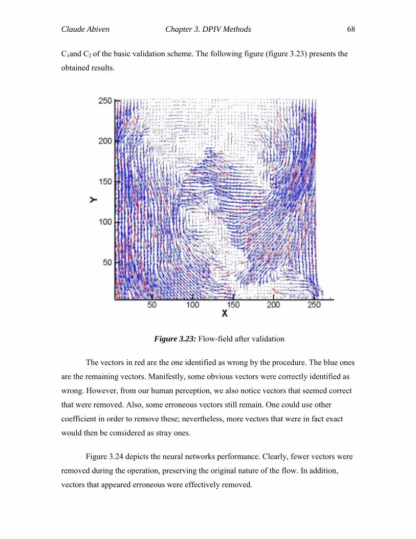
Claude Abiven Chapter 3. DPIV Methods 68
C1and C2 of the basic validation scheme. The following figure (figure 3.23) presents the
obtained results.
Figure 3.23: Flow-field after validation
The vectors in red are the one identified as wrong by the procedure. The blue ones
are the remaining vectors. Manifestly, some obvious vectors were correctly identified as
wrong. However, from our human perception, we also notice vectors that seemed correct
that were removed. Also, some erroneous vectors still remain. One could use other
coefficient in order to remove these; nevertheless, more vectors that were in fact exact
would then be considered as stray ones.
Figure 3.24 depicts the neural networks performance. Clearly, fewer vectors were
removed during the operation, preserving the original nature of the flow. In addition,
vectors that appeared erroneous were effectively removed.
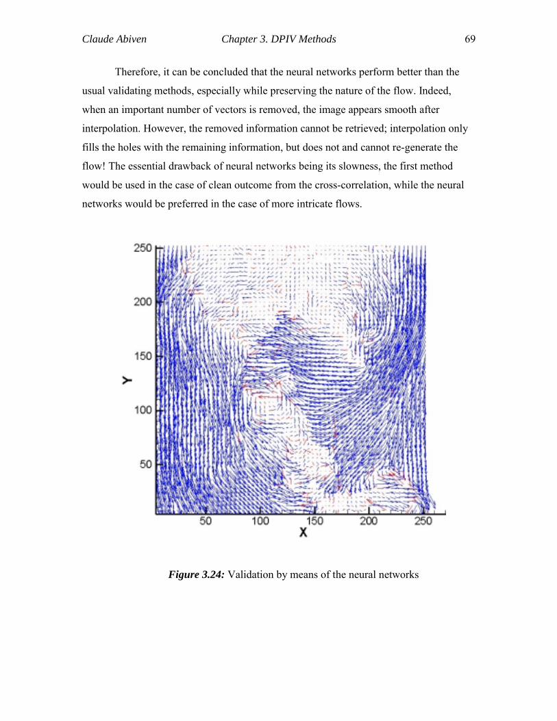
Claude Abiven Chapter 3. DPIV Methods 69
Therefore, it can be concluded that the neural networks perform better than the
usual validating methods, especially while preserving the nature of the flow. Indeed,
when an important number of vectors is removed, the image appears smooth after
interpolation. However, the removed information cannot be retrieved; interpolation only
fills the holes with the remaining information, but does not and cannot re-generate the
flow! The essential drawback of neural networks being its slowness, the first method
would be used in the case of clean outcome from the cross-correlation, while the neural
networks would be preferred in the case of more intricate flows.
Figure 3.24: Validation by means of the neural networks
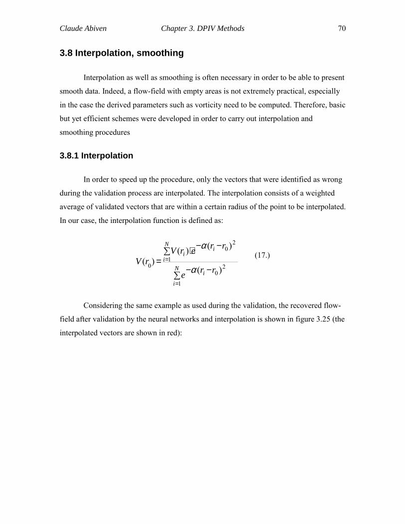
Claude Abiven Chapter 3. DPIV Methods 70
3.8 Interpolation, smoothing
Interpolation as well as smoothing is often necessary in order to be able to present
smooth data. Indeed, a flow-field with empty areas is not extremely practical, especially
in the case the derived parameters such as vorticity need to be computed. Therefore, basic
but yet efficient schemes were developed in order to carry out interpolation and
smoothing procedures
3.8.1 Interpolation
In order to speed up the procedure, only the vectors that were identified as wrong
during the validation process are interpolated. The interpolation consists of a weighted
average of validated vectors that are within a certain radius of the point to be interpolated.
In our case, the interpolation function is defined as:
∑−−
∑−−⋅
=
=
=N
i
i
N
i
ii
rre
rrerVrV
1
20
1
20
0 )(
)()()(
α
α (17.)
Considering the same example as used during the validation, the recovered flow-
field after validation by the neural networks and interpolation is shown in figure 3.25 (the
interpolated vectors are shown in red):
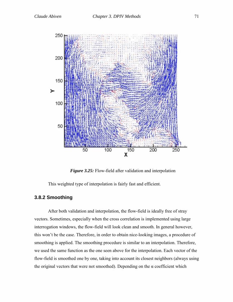
Claude Abiven Chapter 3. DPIV Methods 71
Figure 3.25: Flow-field after validation and interpolation
This weighted type of interpolation is fairly fast and efficient.
3.8.2 Smoothing
After both validation and interpolation, the flow-field is ideally free of stray
vectors. Sometimes, especially when the cross correlation is implemented using large
interrogation windows, the flow-field will look clean and smooth. In general however,
this won’t be the case. Therefore, in order to obtain nice-looking images, a procedure of
smoothing is applied. The smoothing procedure is similar to an interpolation. Therefore,
we used the same function as the one seen above for the interpolation. Each vector of the
flow-field is smoothed one by one, taking into account its closest neighbors (always using
the original vectors that were not smoothed). Depending on the α coefficient which
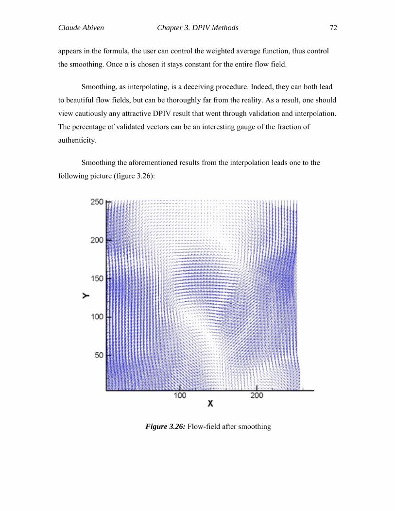
Claude Abiven Chapter 3. DPIV Methods 72
appears in the formula, the user can control the weighted average function, thus control
the smoothing. Once α is chosen it stays constant for the entire flow field.
Smoothing, as interpolating, is a deceiving procedure. Indeed, they can both lead
to beautiful flow fields, but can be thoroughly far from the reality. As a result, one should
view cautiously any attractive DPIV result that went through validation and interpolation.
The percentage of validated vectors can be an interesting gauge of the fraction of
authenticity.
Smoothing the aforementioned results from the interpolation leads one to the
following picture (figure 3.26):
Figure 3.26: Flow-field after smoothing
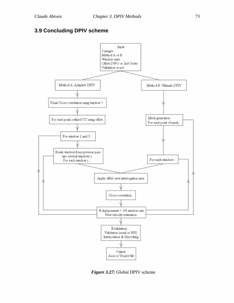
Claude Abiven Chapter 3. DPIV Methods 73
3.9 Concluding DPIV scheme
Figure 3.27: Global DPIV scheme

Claude Abiven Chapter 3. DPIV Methods 74
The algorithm presented in figure 3.27 shows the global DPIV scheme, after
implementation of all the methods discussed in this section. It is to be compared to the
basic system presented at the beginning of this chapter. The method presented here is
much more flexible, and much more accurate, as it will be seen in the following
paragraphs.
75
Chapter 4 DPTV Methods
In this section, we describe a particle-tracking scheme. It consists of two main
steps: an identification of each particle in the flow for the pair of images, followed by a
matching of each particle from the first frame with a particle of the second frame.
4.1 Particle identification
4.1.1 Image processing
In order to distinguish the actual particles present in the flow from noise or other
phases like bubbles, particles, and solid bodies, the image processing tools described in
the second chapter of this report are extremely useful. Depending on the flow properties,
one needs to choose image-processing tools in order to keep as many flow tracers as
possible while removing noise and the other phases. However, a global scheme will be
presented here, which was proved to provide satisfactory results for most test cases.
4.1.1.1. Noise removal
In real cases, the images always present a level of background noise, due to the
camera limitations, the depth of field, the laser beam Gaussian distribution. In order to
distinguish actual particles from noise, one main image-processing tool is commonly
used: the histogram thresholding. This method was previously described in the chapter 2.
4.1.1.2. Big particles segmentation
In the case of the presence of big particles (droplets, bubbles, solid bodies) in the
image, it is necessary to remove these objects, which would appear as a cluster of
particles if they were left in the image. This method, described in the second chapter of
this work, can be used before or after having removed the background noise
Claude Abiven Chapter 4 DPTV Methods 76
4.1.2 Particle identifier
Two different schemes were developed: a standard method similar to the one
proposed by Guezennec and Kiritsis (1990), followed, after analysis, by a maximum
intensity identifier.
4.1.2.1. Guezennec and Kiritsis scheme
We accurately followed the scheme proposed by Guezennec and Kiritsis (1990).
It consists in scanning the image pixel after pixel. For each pixel above a certain
threshold, its four neighbors that were already scanned are examined. If none of them is
above the specified threshold, a new particle number is assigned to the pixel. If they
belong to one single particle, the current pixel is added to the list of pixels that belong to
the particle. In some cases, the neighbor pixels belong to two different particles. In this
last case, the “two” particles are actually one, and need to be reconnected. All the pixels
belonging to one of them have thus to be assigned to the other, as well as the current
pixel. This algorithm is very efficient, and links each pixel of the image above a certain
threshold to a particle.
4.1.2.2. Maximum intensity identifier
A major drawback can be pointed out from the aforementioned method: its
inability to distinguish a single particle from a cluster of particles in case these particles
are very close to each other. In order to overcome this difficulty, we focused on the
maximum intensity locations. Indeed, since a particle intensity distribution can be
assumed to be Gaussian, a maximum must exist. After pre-processing as seen above, each
pixel of the image is scanned using a 3x3 mask. If the center pixel of this mask
corresponds to a local maximum or is saturated, the pixel is set to a saturated value. After
the whole image has been scanned, a threshold is applied in order to keep only the
saturated values. This process leaves only local maxima and plateaus in the image,
leading to the corresponding particles.
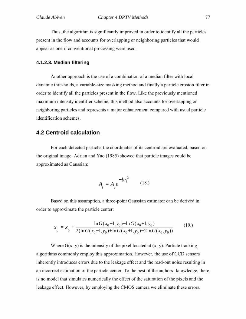
Claude Abiven Chapter 4 DPTV Methods 77
Thus, the algorithm is significantly improved in order to identify all the particles
present in the flow and accounts for overlapping or neighboring particles that would
appear as one if conventional processing were used.
4.1.2.3. Median filtering
Another approach is the use of a combination of a median filter with local
dynamic thresholds, a variable-size masking method and finally a particle erosion filter in
order to identify all the particles present in the flow. Like the previously mentioned
maximum intensity identifier scheme, this method also accounts for overlapping or
neighboring particles and represents a major enhancement compared with usual particle
identification schemes.
4.2 Centroid calculation
For each detected particle, the coordinates of its centroid are evaluated, based on
the original image. Adrian and Yao (1985) showed that particle images could be
approximated as Gaussian:
2
ici
breAA−
= (18.)
Based on this assumption, a three-point Gaussian estimator can be derived in
order to approximate the particle center:
)),(ln2),1(ln),1((ln2),1(ln),1(ln
000000
00000 yxGyxGyxG
yxGyxGxx
c −++−+−−
+= (19.)
Where G(x, y) is the intensity of the pixel located at (x, y). Particle tracking
algorithms commonly employ this approximation. However, the use of CCD sensors
inherently introduces errors due to the leakage effect and the read-out noise resulting in
an incorrect estimation of the particle center. To the best of the authors’ knowledge, there
is no model that simulates numerically the effect of the saturation of the pixels and the
leakage effect. However, by employing the CMOS camera we eliminate these errors.
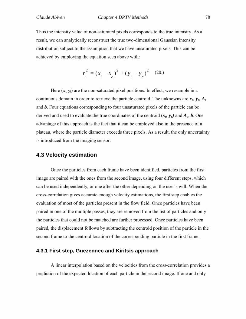
Claude Abiven Chapter 4 DPTV Methods 78
Thus the intensity value of non-saturated pixels corresponds to the true intensity. As a
result, we can analytically reconstruct the true two-dimensional Gaussian intensity
distribution subject to the assumption that we have unsaturated pixels. This can be
achieved by employing the equation seen above with:
222 )()(cicii
yyxxr −+−= (20.)
Here (xi, yi) are the non-saturated pixel positions. In effect, we resample in a
continuous domain in order to retrieve the particle centroid. The unknowns are xc, yc, Ac
and b. Four equations corresponding to four unsaturated pixels of the particle can be
derived and used to evaluate the true coordinates of the centroid (xc, yc) and Ac, b. One
advantage of this approach is the fact that it can be employed also in the presence of a
plateau, where the particle diameter exceeds three pixels. As a result, the only uncertainty
is introduced from the imaging sensor.
4.3 Velocity estimation
Once the particles from each frame have been identified, particles from the first
image are paired with the ones from the second image, using four different steps, which
can be used independently, or one after the other depending on the user’s will. When the
cross-correlation gives accurate enough velocity estimations, the first step enables the
evaluation of most of the particles present in the flow field. Once particles have been
paired in one of the multiple passes, they are removed from the list of particles and only
the particles that could not be matched are further processed. Once particles have been
paired, the displacement follows by subtracting the centroid position of the particle in the
second frame to the centroid location of the corresponding particle in the first frame.
4.3.1 First step, Guezennec and Kiritsis approach
A linear interpolation based on the velocities from the cross-correlation provides a
prediction of the expected location of each particle in the second image. If one and only
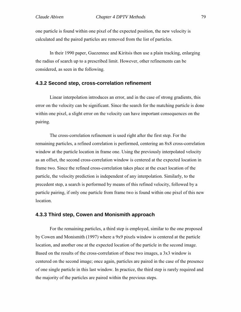
Claude Abiven Chapter 4 DPTV Methods 79
one particle is found within one pixel of the expected position, the new velocity is
calculated and the paired particles are removed from the list of particles.
In their 1990 paper, Guezennec and Kiritsis then use a plain tracking, enlarging
the radius of search up to a prescribed limit. However, other refinements can be
considered, as seen in the following.
4.3.2 Second step, cross-correlation refinement
Linear interpolation introduces an error, and in the case of strong gradients, this
error on the velocity can be significant. Since the search for the matching particle is done
within one pixel, a slight error on the velocity can have important consequences on the
pairing.
The cross-correlation refinement is used right after the first step. For the
remaining particles, a refined correlation is performed, centering an 8x8 cross-correlation
window at the particle location in frame one. Using the previously interpolated velocity
as an offset, the second cross-correlation window is centered at the expected location in
frame two. Since the refined cross-correlation takes place at the exact location of the
particle, the velocity prediction is independent of any interpolation. Similarly, to the
precedent step, a search is performed by means of this refined velocity, followed by a
particle pairing, if only one particle from frame two is found within one pixel of this new
location.
4.3.3 Third step, Cowen and Monismith approach
For the remaining particles, a third step is employed, similar to the one proposed
by Cowen and Monismith (1997) where a 9x9 pixels window is centered at the particle
location, and another one at the expected location of the particle in the second image.
Based on the results of the cross-correlation of these two images, a 3x3 window is
centered on the second image; once again, particles are paired in the case of the presence
of one single particle in this last window. In practice, the third step is rarely required and
the majority of the particles are paired within the previous steps.
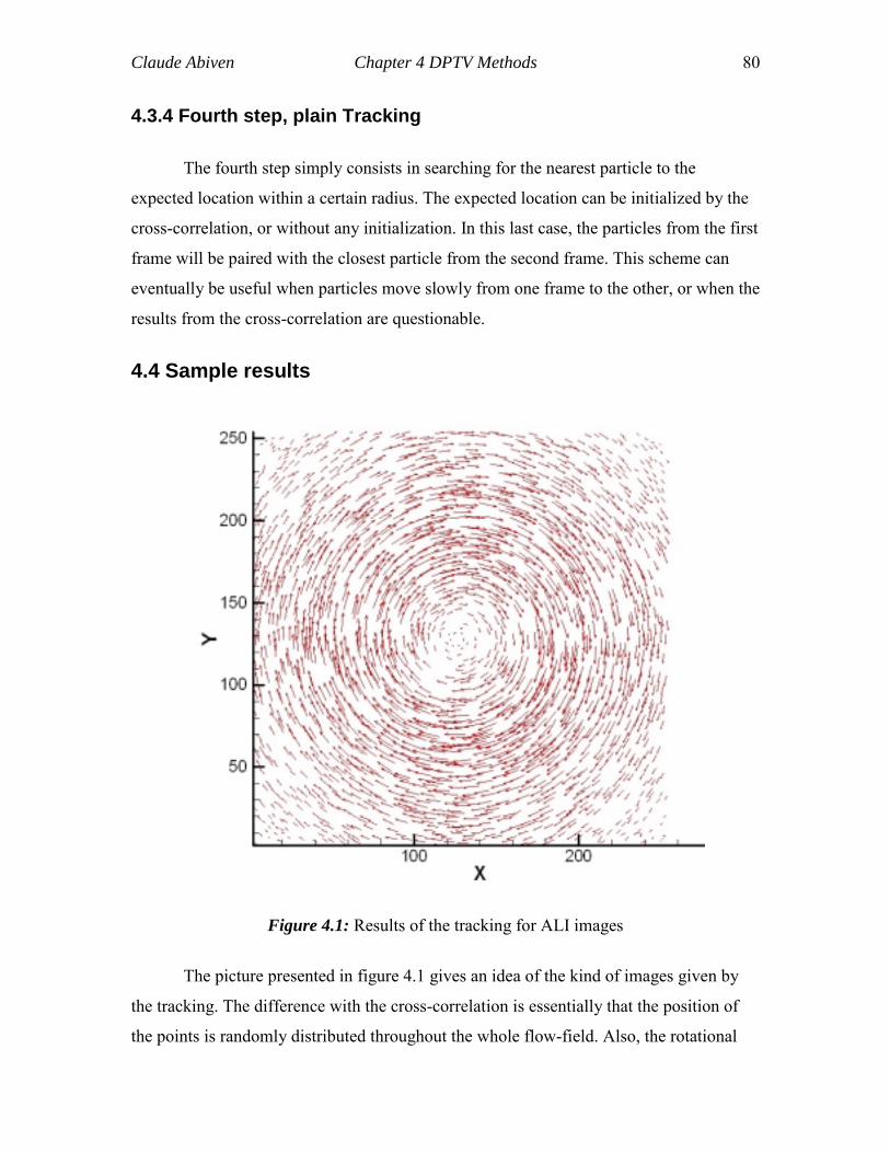
Claude Abiven Chapter 4 DPTV Methods 80
4.3.4 Fourth step, plain Tracking
The fourth step simply consists in searching for the nearest particle to the
expected location within a certain radius. The expected location can be initialized by the
cross-correlation, or without any initialization. In this last case, the particles from the first
frame will be paired with the closest particle from the second frame. This scheme can
eventually be useful when particles move slowly from one frame to the other, or when the
results from the cross-correlation are questionable.
4.4 Sample results
Figure 4.1: Results of the tracking for ALI images
The picture presented in figure 4.1 gives an idea of the kind of images given by
the tracking. The difference with the cross-correlation is essentially that the position of
the points is randomly distributed throughout the whole flow-field. Also, the rotational
Claude Abiven Chapter 4 DPTV Methods 81
character of the flow field is preserved, alleviating the linearity inherent in the cross-
correlation, giving a more representative realization of the flow.
Figure 4.2: Wake of the circular cylinder.
Figure 4.2 is to be compared with the ones given by the cross-correlation. The
figure was obtained after smoothing, which can be used, as well as the validation, along
with the hybrid particle tracking. The natural wavy character of the flow is resolved
generating more physically representative measurements than cross-correlation.
82
Chapter 5 Statistics and comparisons
This chapter is dedicated to the comparisons of the different methods presented in
the two preceding chapters. In order to determine the quality of the proposed
methodologies, Monte-Carlo simulations were preformed for different versions of our
DPIV and DPTV systems, along with one of the best DPIV software’s in the market.
Three major lines of comparisons were defined: uniform displacements, test with
ALI images, and finally peak-locking effect (namely, the tendency of the cross-
correlation evaluation to lock on the closest integer value).
5.1 The compared software
Table 5.1 is referencing the different versions that were compared during this
effort. One section deals with cross-correlation and another with hybrid particle tracking.
Since the particle tracking presented throughout the present work was the only available
version, its performance was discussed comparing it to the cross-correlation schemes.
However, differences between these two methods are significant, so that hybrid and
cross-correlation should be considered as two different and complementary tools rather
than two ways to achieve the same result.
Concerning the cross-correlation, the main implementations investigated were the
basic scheme by Gharib, the version that was developed during this work, and Dantec’s.
Dantec Dynamics is a Danish group, leader in DPIV technology, and their program can
be considered as a top-performing software package used as reference for the following
statistical analyses. Three main interrogation schemes were employed: a 32-32-16
windows system was generally applied, but a scheme employing 64-64-32-16 pixels
interrogation windows was used when expected displacements were above 8 pixels (ALI
images with 8 pixels maximum displacement), and in order to test the performance of the
system in resolving smaller length scales, a 32-32-16-8 method was considered. These
versions were evaluated using the two types of offsets described earlier.
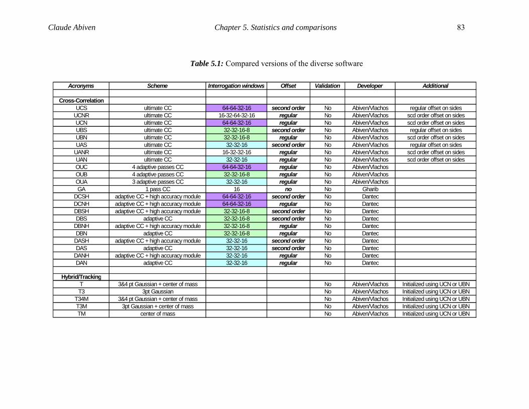
Claude Abiven Chapter 5. Statistics and comparisons 83
Table 5.1: Compared versions of the diverse software
Acronyms Scheme Interrogation windows Offset Validation Developer Additional
Cross-CorrelationUCS ultimate CC 64-64-32-16 second order No Abiven/Vlachos regular offset on sides
UCNR ultimate CC 16-32-64-32-16 regular No Abiven/Vlachos scd order offset on sidesUCN ultimate CC 64-64-32-16 regular No Abiven/Vlachos scd order offset on sidesUBS ultimate CC 32-32-16-8 second order No Abiven/Vlachos regular offset on sidesUBN ultimate CC 32-32-16-8 regular No Abiven/Vlachos scd order offset on sidesUAS ultimate CC 32-32-16 second order No Abiven/Vlachos regular offset on sides
UANR ultimate CC 16-32-32-16 regular No Abiven/Vlachos scd order offset on sidesUAN ultimate CC 32-32-16 regular No Abiven/Vlachos scd order offset on sidesOUC 4 adaptive passes CC 64-64-32-16 regular No Abiven/VlachosOUB 4 adaptive passes CC 32-32-16-8 regular No Abiven/VlachosOUA 3 adaptive passes CC 32-32-16 regular No Abiven/VlachosGA 1 pass CC 16 no No Gharib
DCSH adaptive CC + high accuracy module 64-64-32-16 second order No DantecDCNH adaptive CC + high accuracy module 64-64-32-16 regular No DantecDBSH adaptive CC + high accuracy module 32-32-16-8 second order No DantecDBS adaptive CC 32-32-16-8 second order No Dantec
DBNH adaptive CC + high accuracy module 32-32-16-8 regular No DantecDBN adaptive CC 32-32-16-8 regular No Dantec
DASH adaptive CC + high accuracy module 32-32-16 second order No DantecDAS adaptive CC 32-32-16 second order No Dantec
DANH adaptive CC + high accuracy module 32-32-16 regular No DantecDAN adaptive CC 32-32-16 regular No Dantec
Hybrid/TrackingT 3&4 pt Gaussian + center of mass No Abiven/Vlachos Initialized using UCN or UBNT3 3pt Gaussian No Abiven/Vlachos Initialized using UCN or UBN
T34M 3&4 pt Gaussian + center of mass No Abiven/Vlachos Initialized using UCN or UBNT3M 3pt Gaussian + center of mass No Abiven/Vlachos Initialized using UCN or UBNTM center of mass No Abiven/Vlachos Initialized using UCN or UBN
Claude Abiven Chapter 5. Statistics and comparisons 84
In order to compare the actual repercussion of the ultimate system with the
standard cross-correlation schemes, we analyzed two versions (UCN and OUA) the core
of which was exactly the same, the only difference being that UCN calculates the offset
at the exact same location as the final velocity estimation, while standard cross-
correlation methods break windows into smaller ones, resulting in an approximation of
the offset at a different position than the final evaluation
5.2 Uniform displacements
Two major computer experiments were carried out concerning uniform
displacements: one with interrogation window sizes successively being reduced to 16x16,
and the other to 8x8 pixels. This was necessary due to the difference between the two
schemes. The first one is expected to give a better accuracy. Indeed, more particles are
susceptible to be found within the window, consequently, the final velocity is averaged
taking into account more tracers. On the other hand, smaller windows reduce spatial
averaging effects thus allowing the resolution of smaller length scales.
5.2.1 Uniform displacements resolved with16x16 window size
5.2.1.1. Global performance
A first comparison was carried out with the basic scheme presented in the third
chapter of this work (GA) along with two schemes using the dynamic offset feature
(UAN and DANH), as well as the hybrid technique (T). The results of this comparison
are plotted in figure 5.1. The advantage of the offset is apparent. Indeed, after 0.5 pixels
displacement, the error for the basic scheme (GA) keeps on increasing, while for all the
dynamically adaptive schemes (three other methods) it goes down until the next integer is
reached, and repeats the same pattern independent of the displacement. The mean error
that appears on the right of the figure shows a difference of an order of magnitude
between GA (mean error of 2) and the other schemes (mean errors below 0.1). This
shows the profound influence of the dynamic window offset feature. It also illustrates the
high accuracy of the tracking. Indeed, tracking every particle without any mistake is a
task that is far from easy. Many errors can occur along the way, such as confusing one
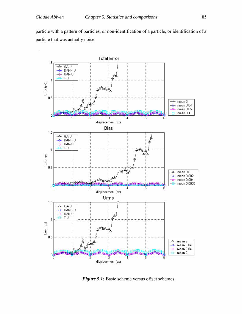
Claude Abiven Chapter 5. Statistics and comparisons 85
particle with a pattern of particles, or non-identification of a particle, or identification of a
particle that was actually noise.
Figure 5.1: Basic scheme versus offset schemes
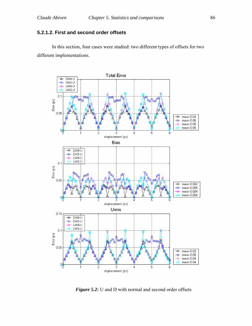
Claude Abiven Chapter 5. Statistics and comparisons 86
5.2.1.2. First and second order offsets
In this section, four cases were studied: two different types of offsets for two
different implementations.
Figure 5.2: U and D with normal and second order offsets
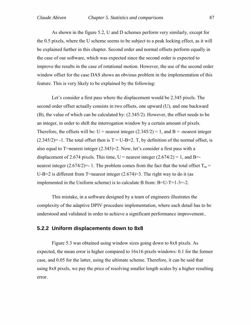
Claude Abiven Chapter 5. Statistics and comparisons 87
As shown in the figure 5.2, U and D schemes perform very similarly, except for
the 0.5 pixels, where the U scheme seems to be subject to a peak locking effect, as it will
be explained further in this chapter. Second order and normal offsets perform equally in
the case of our software, which was expected since the second order is expected to
improve the results in the case of rotational motion. However, the use of the second order
window offset for the case DAS shows an obvious problem in the implementation of this
feature. This is very likely to be explained by the following:
Let’s consider a first pass where the displacement would be 2.345 pixels. The
second order offset actually consists in two offsets, one upward (U), and one backward
(B), the value of which can be calculated by: (2.345/2). However, the offset needs to be
an integer, in order to shift the interrogation window by a certain amount of pixels.
Therefore, the offsets will be: U = nearest integer (2.345/2) = 1, and B = -nearest integer
(2.345/2)= -1. The total offset then is T = U-B=2. T, by definition of the normal offset, is
also equal to T=nearest integer (2.345)=2. Now, let’s consider a first pass with a
displacement of 2.674 pixels. This time, U = nearest integer (2.674/2) = 1, and B=-
nearest integer (2.674/2)=- 1. The problem comes from the fact that the total offset Tm =
U-B=2 is different from T=nearest integer (2.674)=3. The right way to do it (as
implemented in the Uniform scheme) is to calculate B from: B=U-T=1-3=-2.
This mistake, in a software designed by a team of engineers illustrates the
complexity of the adaptive DPIV procedure implementation, where each detail has to be
understood and validated in order to achieve a significant performance improvement..
5.2.2 Uniform displacements down to 8x8
Figure 5.3 was obtained using window sizes going down to 8x8 pixels. As
expected, the mean error is higher compared to 16x16 pixels windows: 0.1 for the former
case, and 0.05 for the latter, using the ultimate scheme. Therefore, it can be said that
using 8x8 pixels, we pay the price of resolving smaller length scales by a higher resulting
error.
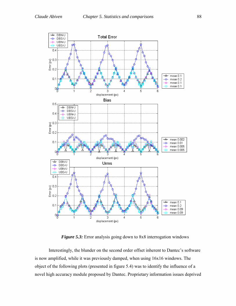
Claude Abiven Chapter 5. Statistics and comparisons 88
Figure 5.3: Error analysis going down to 8x8 interrogation windows
Interestingly, the blunder on the second order offset inherent to Dantec’s software
is now amplified, while it was previously damped, when using 16x16 windows. The
object of the following plots (presented in figure 5.4) was to identify the influence of a
novel high accuracy module proposed by Dantec. Proprietary information issues deprived
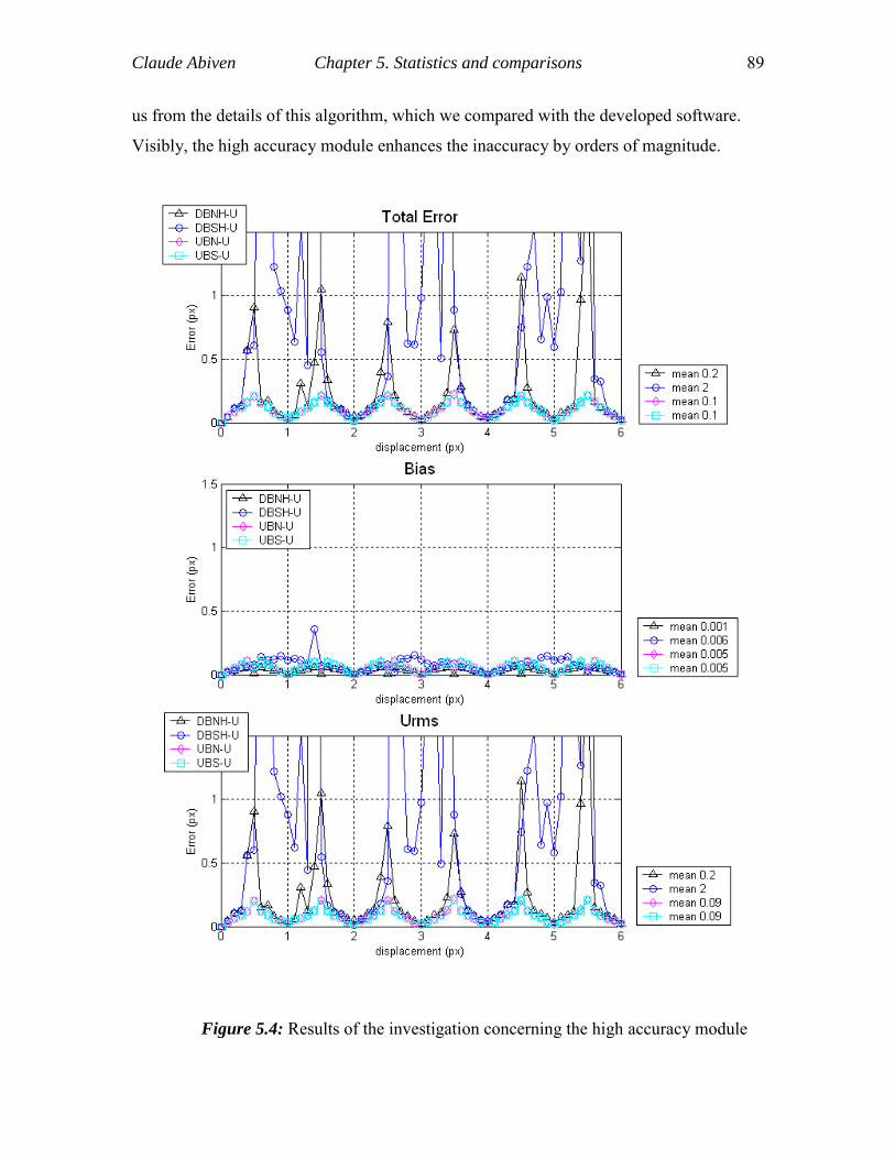
Claude Abiven Chapter 5. Statistics and comparisons 89
us from the details of this algorithm, which we compared with the developed software.
Visibly, the high accuracy module enhances the inaccuracy by orders of magnitude.
Figure 5.4: Results of the investigation concerning the high accuracy module
Claude Abiven Chapter 5. Statistics and comparisons 90
5.2.3 Comparisons of several versions of the developed software
As it can be observed from figure 5.5, results from one version of the software we
developed to the other show significant consistency.
Figure 5.5: Several versions of the developed software
Claude Abiven Chapter 5. Statistics and comparisons 91
This was expected, due to the uniform flow field that was the object of this
analysis. Indeed, the second order offset is not supposed to perform better than the
regular offset in this case (but not worse either), neither is the ultimate scheme versus the
adaptive (OUA) version. The tracking scheme presents a highest error, with a mean of
0.1 versus 0.05 for the cross-correlation. However, it needs to be emphasized that the
hybrid gives the same results when initialized with data obtained using 16x16 and 8x8
windows. Therefore, the use of 16x16 windows in order to initialize the tracking scheme
seems to prevail here. Indeed, using smaller windows implies more inaccuracy in the
results as well as computational inefficiency. Also, let’s highlight the fact that the mean
error is nearly zero while the total error is primarily attribute to random error. This
element implies an alleviation of the peak locking effects (this will be discussed in detail
in a following paragraph), which by it self is a significant improvement on the accuracy
of the system.
5.2.4 Particle-tracking
Figure 5.6 shows a larger error when a center of mass is used as an identifier (For
the TM case, the centroid of a particle is calculated based on a center of mass of the
pixels belonging to this particle). The smallest error was obtained without any center of
mass identification (T34 scheme), but also without taking into account particles with
several saturated pixels. The only way we found to resolve them accurately was by using
a center of mass.
The difference between T34M and T34 is small, especially if we consider the fact
that T34 tracks only those particles with a maximum of one non-saturated pixel, while
T34M tracks every possible one. However, the use of T34M takes more particles into
consideration, since centroids of particles without any saturated pixel (resolved using a 3
points Gaussian estimator), particles with a single saturated pixel (resolved using a 4
points Gaussian estimator), and particles with several saturated pixels (resolved using a
center of mass) are identified.
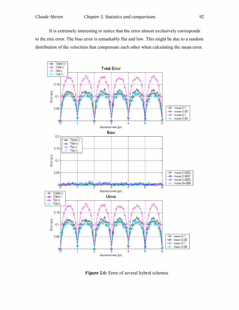
Claude Abiven Chapter 5. Statistics and comparisons 92
It is extremely interesting to notice that the error almost exclusively corresponds
to the rms error. The bias error is remarkably flat and low. This might be due to a random
distribution of the velocities that compensate each other when calculating the mean error.
Figure 5.6: Error of several hybrid schemes
Claude Abiven Chapter 5. Statistics and comparisons 93
5.2.5 Concluding remarks concerning the uniform statistical analyses
In this section, we have seen the uncontestable superiority of schemes that include
the dynamic window offset. Our software performs well in every case, although affected
by the peak locking effect as shown by the important error that appears for every 0.5
pixels displacement in the Urms error represented in figure 5.5. The peak-locking effect
will be discussed later in this chapter. Clearly, Dantec’s software presents major
implementation weaknesses, although their best results consistently give a better
estimation of the flow field. The tracking scheme provides interesting outcomes, even
though the centroid estimation might need improvement.
5.3 Comparisons using ALI images
As discussed in chapter two, we chose a graphical approach in order to quantify
the error using ALI images. In this case, differences are expected between the different
versions. Although rms, bias, and total errors were plotted for two categories of ALI
images, the graphical comparison presented here is limited to the total error for ALI
images with a maximum displacement of 8 pixels. A table providing the result for all the
studied cases is presented in section 5.3.2. The total error was calculated taking into
account the x-component of the velocity. Similar results were obtained considering the y-
component.
The objective of this type of comparisons was to provide information on both the
amplitude of the error and the distribution of this error throughout the flow-field. Indeed,
for ALI images, the highest gradient was located in the core of the vortex, so high errors
were expected there, as well as at the points were the velocity reaches a maximum, since
at this location, the velocity increases, reaches the peak, and then decreases, providing a
maximum point along with two different velocity gradients.
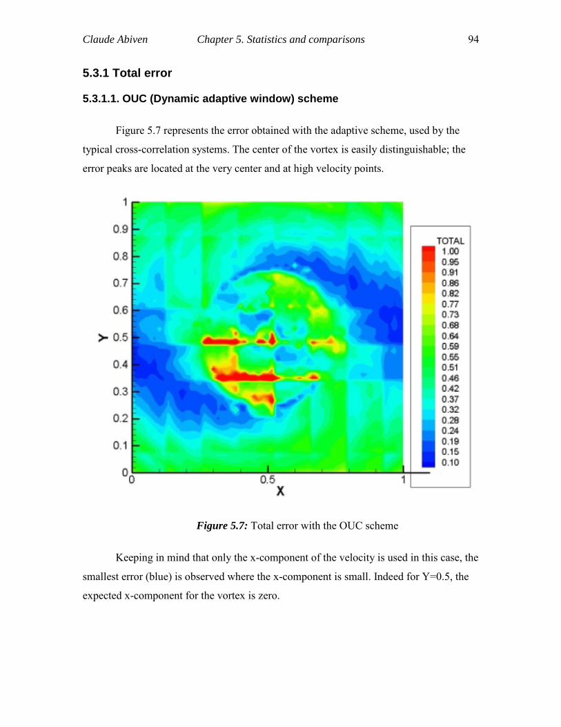
Claude Abiven Chapter 5. Statistics and comparisons 94
5.3.1 Total error
5.3.1.1. OUC (Dynamic adaptive window) scheme
Figure 5.7 represents the error obtained with the adaptive scheme, used by the
typical cross-correlation systems. The center of the vortex is easily distinguishable; the
error peaks are located at the very center and at high velocity points.
Figure 5.7: Total error with the OUC scheme
Keeping in mind that only the x-component of the velocity is used in this case, the
smallest error (blue) is observed where the x-component is small. Indeed for Y=0.5, the
expected x-component for the vortex is zero.
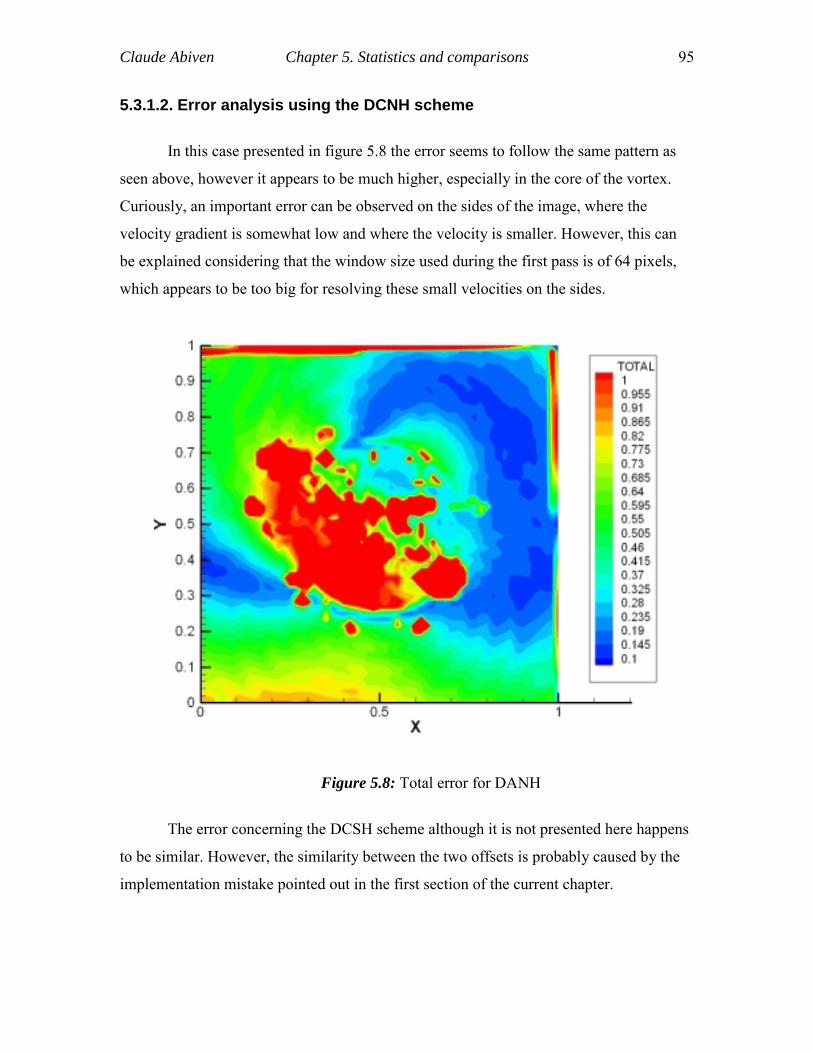
Claude Abiven Chapter 5. Statistics and comparisons 95
5.3.1.2. Error analysis using the DCNH scheme
In this case presented in figure 5.8 the error seems to follow the same pattern as
seen above, however it appears to be much higher, especially in the core of the vortex.
Curiously, an important error can be observed on the sides of the image, where the
velocity gradient is somewhat low and where the velocity is smaller. However, this can
be explained considering that the window size used during the first pass is of 64 pixels,
which appears to be too big for resolving these small velocities on the sides.
Figure 5.8: Total error for DANH
The error concerning the DCSH scheme although it is not presented here happens
to be similar. However, the similarity between the two offsets is probably caused by the
implementation mistake pointed out in the first section of the current chapter.
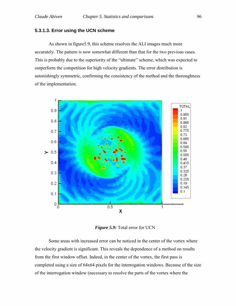
Claude Abiven Chapter 5. Statistics and comparisons 96
5.3.1.3. Error using the UCN scheme
As shown in figure5.9, this scheme resolves the ALI images much more
accurately. The pattern is now somewhat different than that for the two previous cases.
This is probably due to the superiority of the “ultimate” scheme, which was expected to
outperform the competition for high velocity gradients. The error distribution is
astonishingly symmetric, confirming the consistency of the method and the thoroughness
of the implementation.
Figure 5.9: Total error for UCN
Some areas with increased error can be noticed in the center of the vortex where
the velocity gradient is significant. This reveals the dependence of a method on results
from the first window offset. Indeed, in the center of the vortex, the first pass is
completed using a size of 64x64 pixels for the interrogation windows. Because of the size
of the interrogation window (necessary to resolve the parts of the vortex where the
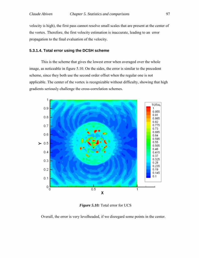
Claude Abiven Chapter 5. Statistics and comparisons 97
velocity is high), the first pass cannot resolve small scales that are present at the center of
the vortex. Therefore, the first velocity estimation is inaccurate, leading to an error
propagation to the final evaluation of the velocity.
5.3.1.4. Total error using the DCSH scheme
This is the scheme that gives the lowest error when averaged over the whole
image, as noticeable in figure 5.10. On the sides, the error is similar to the precedent
scheme, since they both use the second order offset when the regular one is not
applicable. The center of the vortex is recognizable without difficulty, showing that high
gradients seriously challenge the cross-correlation schemes.
Figure 5.10: Total error for UCS
Overall, the error is very levelheaded, if we disregard some points in the center.
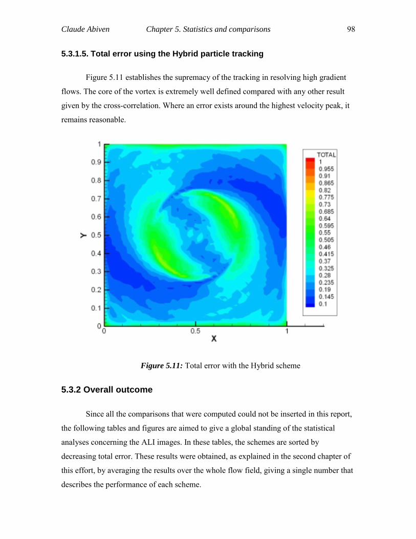
Claude Abiven Chapter 5. Statistics and comparisons 98
5.3.1.5. Total error using the Hybrid particle tracking
Figure 5.11 establishes the supremacy of the tracking in resolving high gradient
flows. The core of the vortex is extremely well defined compared with any other result
given by the cross-correlation. Where an error exists around the highest velocity peak, it
remains reasonable.
Figure 5.11: Total error with the Hybrid scheme
5.3.2 Overall outcome
Since all the comparisons that were computed could not be inserted in this report,
the following tables and figures are aimed to give a global standing of the statistical
analyses concerning the ALI images. In these tables, the schemes are sorted by
decreasing total error. These results were obtained, as explained in the second chapter of
this effort, by averaging the results over the whole flow field, giving a single number that
describes the performance of each scheme.
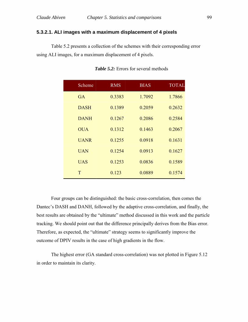
Claude Abiven Chapter 5. Statistics and comparisons 99
5.3.2.1. ALI images with a maximum displacement of 4 pixels
Table 5.2 presents a collection of the schemes with their corresponding error
using ALI images, for a maximum displacement of 4 pixels.
Table 5.2: Errors for several methods
Scheme RMS BIAS TOTAL
GA 0.3383 1.7092 1.7866
DASH 0.1389 0.2059 0.2632
DANH 0.1267 0.2086 0.2584
OUA 0.1312 0.1463 0.2067
UANR 0.1255 0.0918 0.1631
UAN 0.1254 0.0913 0.1627
UAS 0.1253 0.0836 0.1589
T 0.123 0.0889 0.1574
Four groups can be distinguished: the basic cross-correlation, then comes the
Dantec’s DASH and DANH, followed by the adaptive cross-correlation, and finally, the
best results are obtained by the “ultimate” method discussed in this work and the particle
tracking. We should point out that the difference principally derives from the Bias error.
Therefore, as expected, the “ultimate” strategy seems to significantly improve the
outcome of DPIV results in the case of high gradients in the flow.
The highest error (GA standard cross-correlation) was not plotted in Figure 5.12
in order to maintain its clarity.
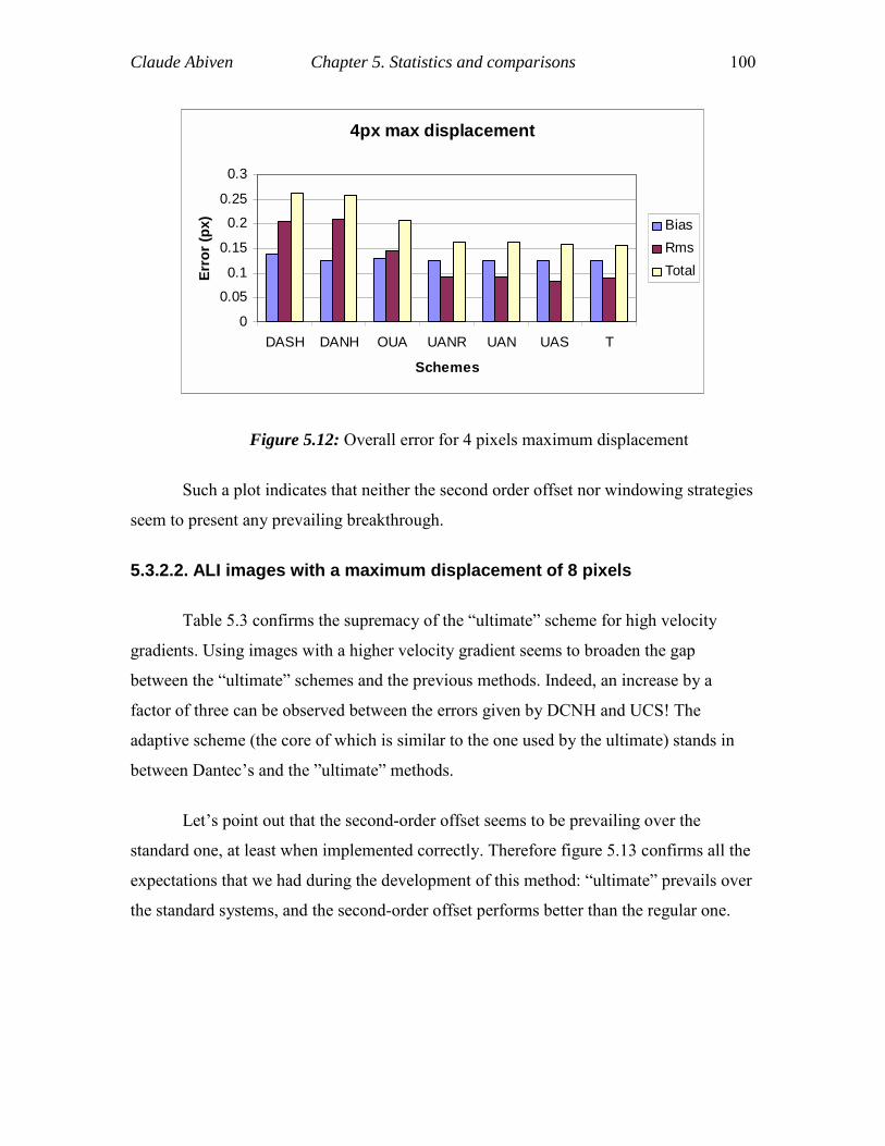
Claude Abiven Chapter 5. Statistics and comparisons 100
4px max displacement
0
0.050.1
0.15
0.20.25
0.3
DASH DANH OUA UANR UAN UAS T
Schemes
Erro
r (px
) BiasRmsTotal
Figure 5.12: Overall error for 4 pixels maximum displacement
Such a plot indicates that neither the second order offset nor windowing strategies
seem to present any prevailing breakthrough.
5.3.2.2. ALI images with a maximum displacement of 8 pixels
Table 5.3 confirms the supremacy of the “ultimate” scheme for high velocity
gradients. Using images with a higher velocity gradient seems to broaden the gap
between the “ultimate” schemes and the previous methods. Indeed, an increase by a
factor of three can be observed between the errors given by DCNH and UCS! The
adaptive scheme (the core of which is similar to the one used by the ultimate) stands in
between Dantec’s and the ”ultimate” methods.
Let’s point out that the second-order offset seems to be prevailing over the
standard one, at least when implemented correctly. Therefore figure 5.13 confirms all the
expectations that we had during the development of this method: “ultimate” prevails over
the standard systems, and the second-order offset performs better than the regular one.
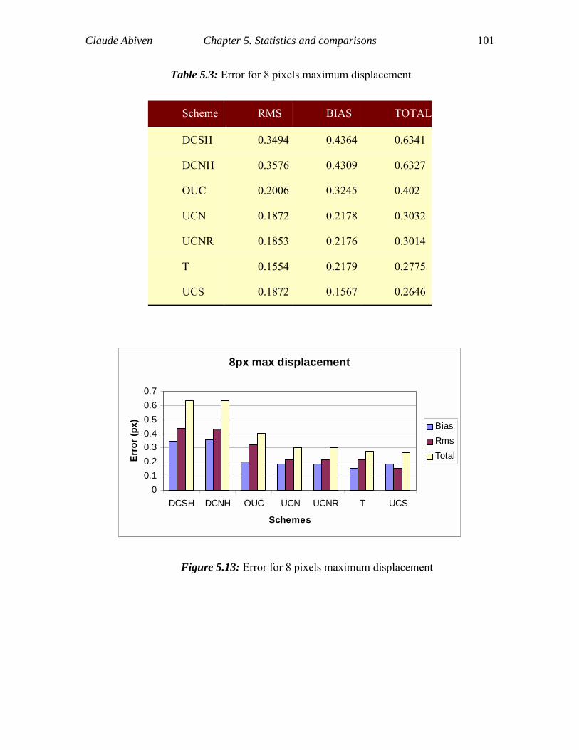
Claude Abiven Chapter 5. Statistics and comparisons 101
Table 5.3: Error for 8 pixels maximum displacement
Scheme RMS BIAS TOTAL
DCSH 0.3494 0.4364 0.6341
DCNH 0.3576 0.4309 0.6327
OUC 0.2006 0.3245 0.402
UCN 0.1872 0.2178 0.3032
UCNR 0.1853 0.2176 0.3014
T 0.1554 0.2179 0.2775
UCS 0.1872 0.1567 0.2646
8px max displacement
00.10.20.30.40.50.60.7
DCSH DCNH OUC UCN UCNR T UCS
Schemes
Erro
r (px
)
BiasRmsTotal
Figure 5.13: Error for 8 pixels maximum displacement
Claude Abiven Chapter 5. Statistics and comparisons 102
5.4 Peak locking effect
5.4.1 Definition
Right after having cross-correlated two images, it is necessary to estimate the
position of the cross-correlation peak in order to determine the displacement. Since a
pixel is the smallest unit in a digital image, one could consider reasonable to take the
center of the highest intensity pixel as the cross-correlation peak. However, in order to
achieve sub-pixel accuracy, not only the highest intensity peak, but also its neighborhood
need to be considered. Methods have been developed, like for example Gaussian fit
estimators, which provide a better approximation to the peak location. Nevertheless, this
last method has a tendency to “lock” on the nearest integer value in the neighborhood of
the peak, resulting in erroneous and biased velocity estimations.
Therefore, in order to quantify this effect, we carried out an analysis for our data
as well as Dantec’s who claim their software is not subject to peak locking.
The procedure for the peak locking estimation is quite straightforward: Based on
the results of the uniform displacement images, we scanned each data file for velocities
ranging from zero to one pixel displacement. The scale from zero to one pixel was then
divided into twenty sections the width of which was 0.05 pixels. The histogram of each
velocity value within the intervals was then constructed. Without any peak locking effect,
the number of velocities in each section should have been the same.
5.4.2 Results of the analysis
5.4.2.1. Comparison of the general cases
First we performed the analysis considering the general cases: G16, UAN,
DANH, and the Hybrid scheme T34M:
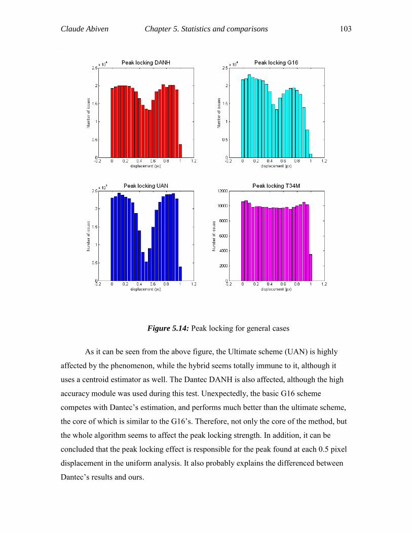
Claude Abiven Chapter 5. Statistics and comparisons 103
Figure 5.14: Peak locking for general cases
As it can be seen from the above figure, the Ultimate scheme (UAN) is highly
affected by the phenomenon, while the hybrid seems totally immune to it, although it
uses a centroid estimator as well. The Dantec DANH is also affected, although the high
accuracy module was used during this test. Unexpectedly, the basic G16 scheme
competes with Dantec’s estimation, and performs much better than the ultimate scheme,
the core of which is similar to the G16’s. Therefore, not only the core of the method, but
the whole algorithm seems to affect the peak locking strength. In addition, it can be
concluded that the peak locking effect is responsible for the peak found at each 0.5 pixel
displacement in the uniform analysis. It also probably explains the differenced between
Dantec’s results and ours.
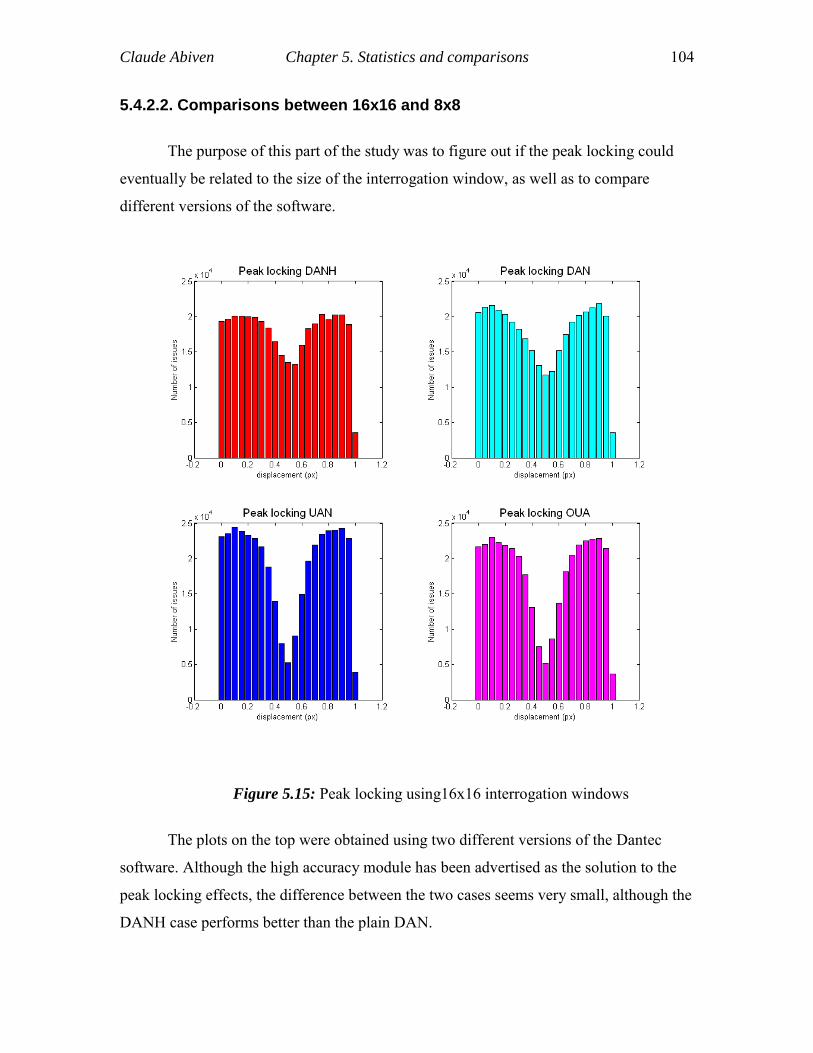
Claude Abiven Chapter 5. Statistics and comparisons 104
5.4.2.2. Comparisons between 16x16 and 8x8
The purpose of this part of the study was to figure out if the peak locking could
eventually be related to the size of the interrogation window, as well as to compare
different versions of the software.
Figure 5.15: Peak locking using16x16 interrogation windows
The plots on the top were obtained using two different versions of the Dantec
software. Although the high accuracy module has been advertised as the solution to the
peak locking effects, the difference between the two cases seems very small, although the
DANH case performs better than the plain DAN.
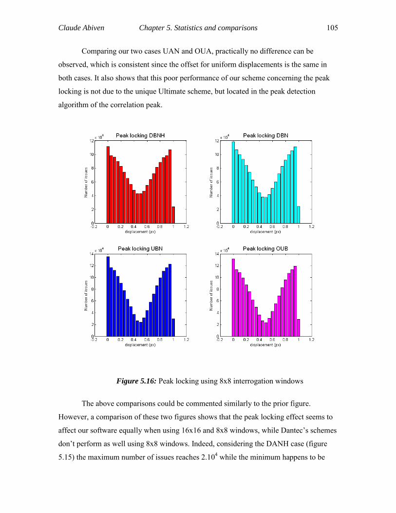
Claude Abiven Chapter 5. Statistics and comparisons 105
Comparing our two cases UAN and OUA, practically no difference can be
observed, which is consistent since the offset for uniform displacements is the same in
both cases. It also shows that this poor performance of our scheme concerning the peak
locking is not due to the unique Ultimate scheme, but located in the peak detection
algorithm of the correlation peak.
Figure 5.16: Peak locking using 8x8 interrogation windows
The above comparisons could be commented similarly to the prior figure.
However, a comparison of these two figures shows that the peak locking effect seems to
affect our software equally when using 16x16 and 8x8 windows, while Dantec’s schemes
don’t perform as well using 8x8 windows. Indeed, considering the DANH case (figure
5.15) the maximum number of issues reaches 2.104 while the minimum happens to be
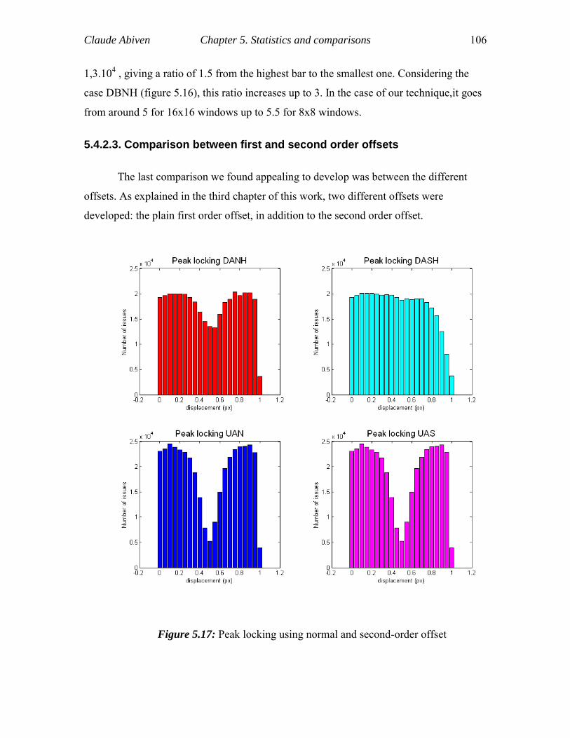
Claude Abiven Chapter 5. Statistics and comparisons 106
1,3.104 , giving a ratio of 1.5 from the highest bar to the smallest one. Considering the
case DBNH (figure 5.16), this ratio increases up to 3. In the case of our technique,it goes
from around 5 for 16x16 windows up to 5.5 for 8x8 windows.
5.4.2.3. Comparison between first and second order offsets
The last comparison we found appealing to develop was between the different
offsets. As explained in the third chapter of this work, two different offsets were
developed: the plain first order offset, in addition to the second order offset.
Figure 5.17: Peak locking using normal and second-order offset

Claude Abiven Chapter 5. Statistics and comparisons 107
The above results show similar results in our case for both offsets. However, in
the case of Dantec’s, the second offset coupled with the high accuracy module seems to
perform remarkably well. However, given the results obtained in the first part of these
comparisons, one will remember that the second order offset didn’t seem to be well
implemented in the case of Dantec’s schemes. Therefore, this absence of peak locking
might be counter balanced by this error.
5.4.3 Concluding remarks concerning the peak locking effect
In summary, it can be inferred from these analyses that the peak locking effect
affects less Dantec’s software than our method. In order to reduce the overall current
errors of our software,further research in this area might be necessary. Also, velocity
evaluation using the tracking is unaffected by this phenomenon, although it also uses a
centroid estimator.
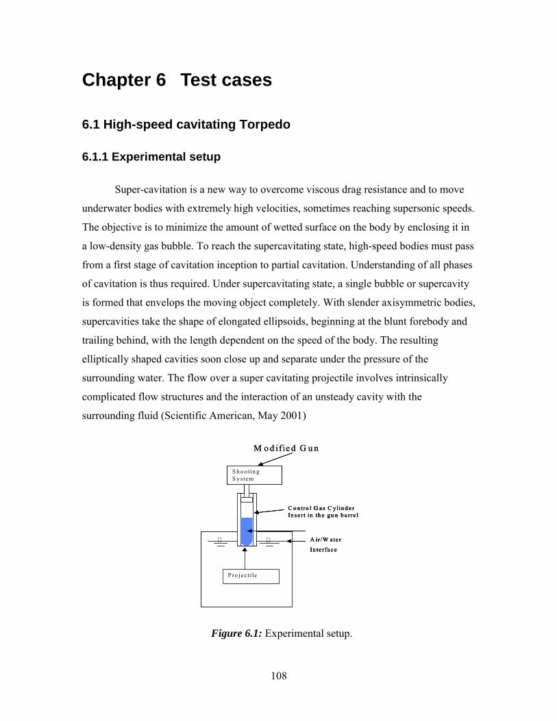
108
Chapter 6 Test cases
6.1 High-speed cavitating Torpedo
6.1.1 Experimental setup
Super-cavitation is a new way to overcome viscous drag resistance and to move
underwater bodies with extremely high velocities, sometimes reaching supersonic speeds.
The objective is to minimize the amount of wetted surface on the body by enclosing it in
a low-density gas bubble. To reach the supercavitating state, high-speed bodies must pass
from a first stage of cavitation inception to partial cavitation. Understanding of all phases
of cavitation is thus required. Under supercavitating state, a single bubble or supercavity
is formed that envelops the moving object completely. With slender axisymmetric bodies,
supercavities take the shape of elongated ellipsoids, beginning at the blunt forebody and
trailing behind, with the length dependent on the speed of the body. The resulting
elliptically shaped cavities soon close up and separate under the pressure of the
surrounding water. The flow over a super cavitating projectile involves intrinsically
complicated flow structures and the interaction of an unsteady cavity with the
surrounding fluid (Scientific American, May 2001)
P ro je c ti le
A ir /W a te r
In te r fa c e
C o n tro l G a s C y lin d e rIn s e r t in th e gu n b a rre l
S h o o tin g S ys te m
∇∇
M o d ifie d G u n
P ro je c ti le
A ir /W a te r
In te r fa c e
C o n tro l G a s C y lin d e rIn s e r t in th e gu n b a rre l
S h o o tin g S ys te m
∇∇
P ro je c ti le
A ir /W a te r
In te r fa c e
C o n tro l G a s C y lin d e rIn s e r t in th e gu n b a rre l
S h o o tin g S ys te m
∇∇
M o d ifie d G u n
Figure 6.1: Experimental setup.
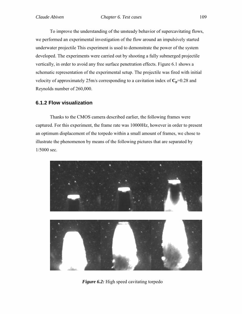
Claude Abiven Chapter 6. Test cases 109
To improve the understanding of the unsteady behavior of supercavitating flows,
we performed an experimental investigation of the flow around an impulsively started
underwater projectile This experiment is used to demonstrate the power of the system
developed. The experiments were carried out by shooting a fully submerged projectile
vertically, in order to avoid any free surface penetration effects. Figure 6.1 shows a
schematic representation of the experimental setup. The projectile was fired with initial
velocity of approximately 25m/s corresponding to a cavitation index of Cp=0.28 and
Reynolds number of 260,000.
6.1.2 Flow visualization
Thanks to the CMOS camera described earlier, the following frames were
captured. For this experiment, the frame rate was 10000Hz, however in order to present
an optimum displacement of the torpedo within a small amount of frames, we chose to
illustrate the phenomenon by means of the following pictures that are separated by
1/5000 sec.
Figure 6.2: High speed cavitating torpedo
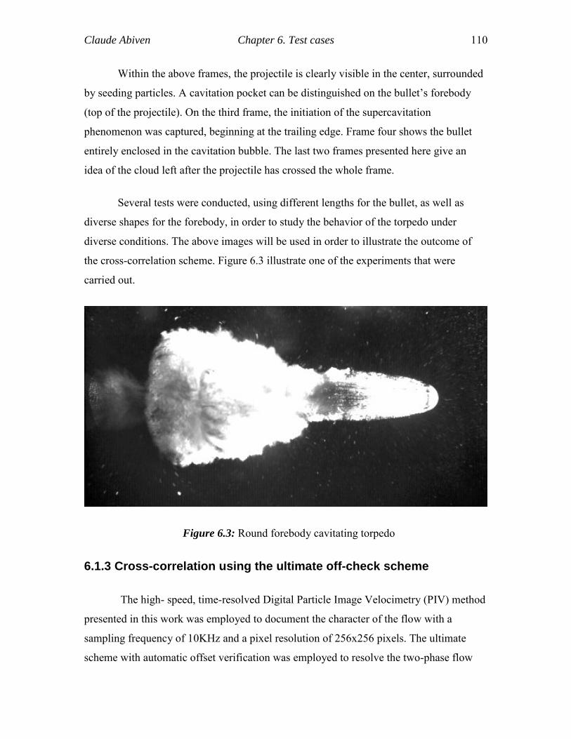
Claude Abiven Chapter 6. Test cases 110
Within the above frames, the projectile is clearly visible in the center, surrounded
by seeding particles. A cavitation pocket can be distinguished on the bullet’s forebody
(top of the projectile). On the third frame, the initiation of the supercavitation
phenomenon was captured, beginning at the trailing edge. Frame four shows the bullet
entirely enclosed in the cavitation bubble. The last two frames presented here give an
idea of the cloud left after the projectile has crossed the whole frame.
Several tests were conducted, using different lengths for the bullet, as well as
diverse shapes for the forebody, in order to study the behavior of the torpedo under
diverse conditions. The above images will be used in order to illustrate the outcome of
the cross-correlation scheme. Figure 6.3 illustrate one of the experiments that were
carried out.
Figure 6.3: Round forebody cavitating torpedo
6.1.3 Cross-correlation using the ultimate off-check scheme
The high- speed, time-resolved Digital Particle Image Velocimetry (PIV) method
presented in this work was employed to document the character of the flow with a
sampling frequency of 10KHz and a pixel resolution of 256x256 pixels. The ultimate
scheme with automatic offset verification was employed to resolve the two-phase flow
Claude Abiven Chapter 6. Test cases 111
velocity distributions and the shape of the cavitation bubble. The speed at which the
bullet travels presents a challeng that is accounted for by the CMOS camera. However,
the images are hardly fitted for cross-correlation. Indeed, the cavitation phenomenon
produces an important amount of steam, that reflects light, introducing noise, clearly
visible when comparing the three images at the top of the figure flow visualization
presented above with the ones at the bottom. The former appear darker than the latter.
Besides the cavitation pocket(s) may introduce erroneous vectors during the cross-
correlation process. Pre-processing was employed in the past in order to remove the
cavitation bubble. However, this process is delicate in the present case. Indeed, still
considering the three top images presented figure 6.2, the forebody of the torpedo is
easily detectable; however the same cannot be said about the aft , which is barely
different from the rest of the image. Consequently, ordinary cross-correlation systems
generate erroneous vectors (that might correspond to the speed of the torpedo itself) that
are scarcely detectable by any kind of validation method due to their quantity.
The following flow-fields were directly obtained from the ultimate system with
automatic offset validation, without any parasite pre-processing operation. The velocity
vectors appear in purple, along with the corresponding cyan streamlines. The presence of
saturated pixels due to the large steam pockets, as well as the moving boundaries and the
speed of the particles were expected to challenge the method.
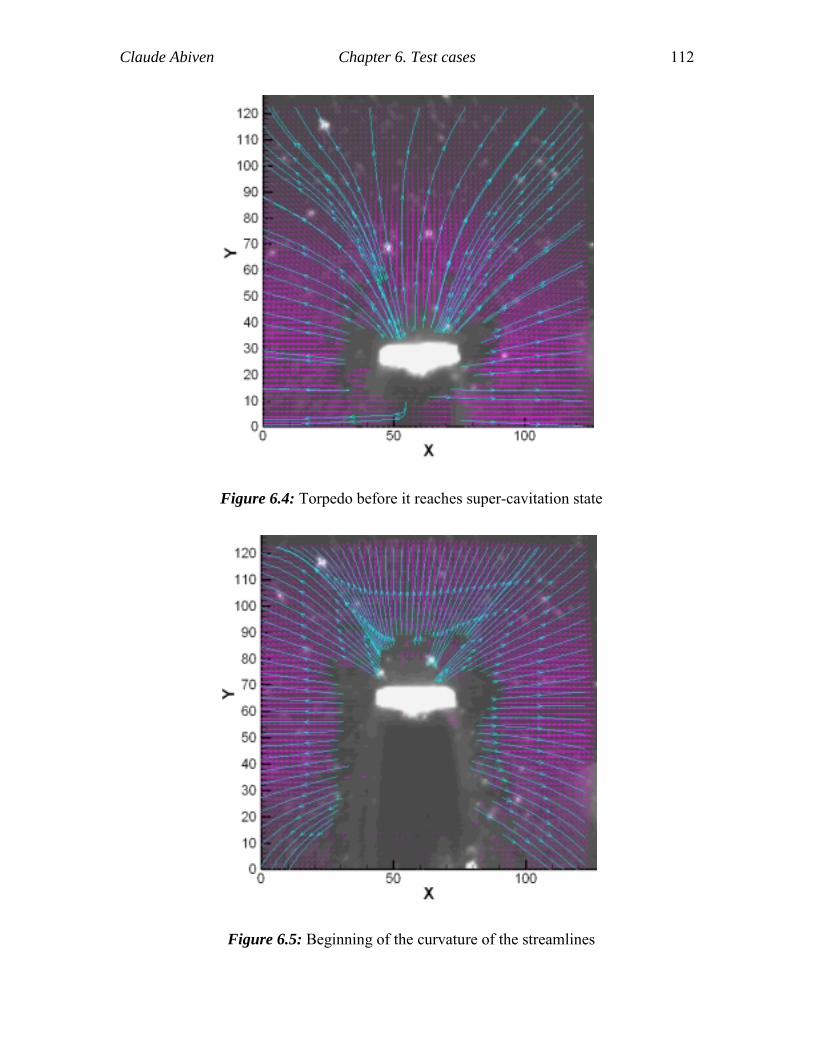
Claude Abiven Chapter 6. Test cases 112
Figure 6.4: Torpedo before it reaches super-cavitation state
Figure 6.5: Beginning of the curvature of the streamlines
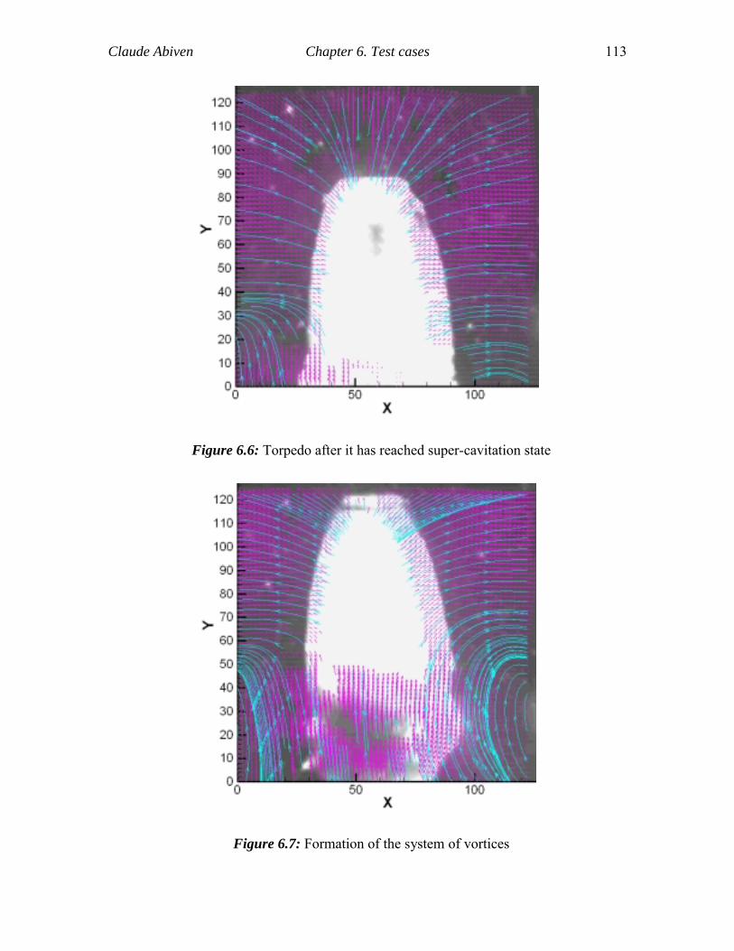
Claude Abiven Chapter 6. Test cases 113
Figure 6.6: Torpedo after it has reached super-cavitation state
Figure 6.7: Formation of the system of vortices
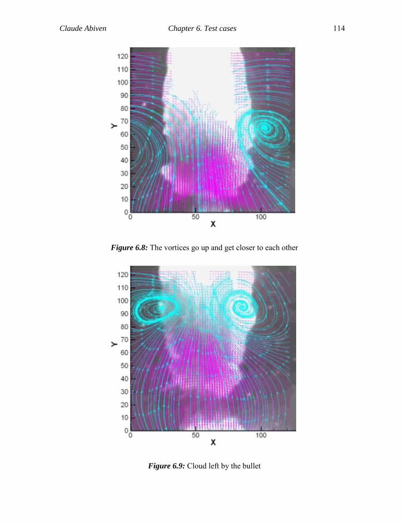
Claude Abiven Chapter 6. Test cases 114
Figure 6.8: The vortices go up and get closer to each other
Figure 6.9: Cloud left by the bullet
Claude Abiven Chapter 6. Test cases 115
This experiment shows the power of the proposed methodology, which
automatically detects the erroneous offsets due to the presence of steam, in conjunction
with an automatic choice of the window size in order to correctly compute the offset
value.
6.2 Spray atomization experiment
6.2.1 Experimental setup
The second case is a spray atomization experiment, recorded with 10KHz
sampling rate by employing a similar experimental setup. The high-pressure spray was
generated using a 60deg cone angle nozzle and a pressure of approximately 10Psi was
applied. A low-speed, annular co-flow was introduced but was not seeded. In addition the
spray was dynamically driven with a frequency of 10Hz. The objective of this pilot
experiment was to demonstrate the ability of the system to resolve a poly-dispersed
distribution by resolving the individual velocities of the droplets.
6.2.2 Challenges and corresponding strategy
Due to the feeble amount of tracers (that are the droplets themselves) visible
within the original images, together with the presence of parasite elements that both the
cone and the spray ligament represent, this experiment was expected to puzzle the cross-
correlation. Indeed, when in presence of a small number of particles, only large
interrogation windows can be employed in order to obtain a reasonable signal. Therefore,
this jeopardizes the resolution of small velocity variation scales. Moreover, and similarly
to the case involving the torpedoes, confusion between the cone and actual particles by
the cross-correlation can be anticipated, originating erroneous velocities.
Therefore, the following strategy was employed: first, image-processing tools
were employed in order to dispose the parasite elements that were background noise,
cone and ligaments. Although the number of remaining particles was small, a cross-
correlation was performed using these pre-processed images, so as to provide an
initialization for the tracking. Finally, the hybrid DPTV was employed with the purpose
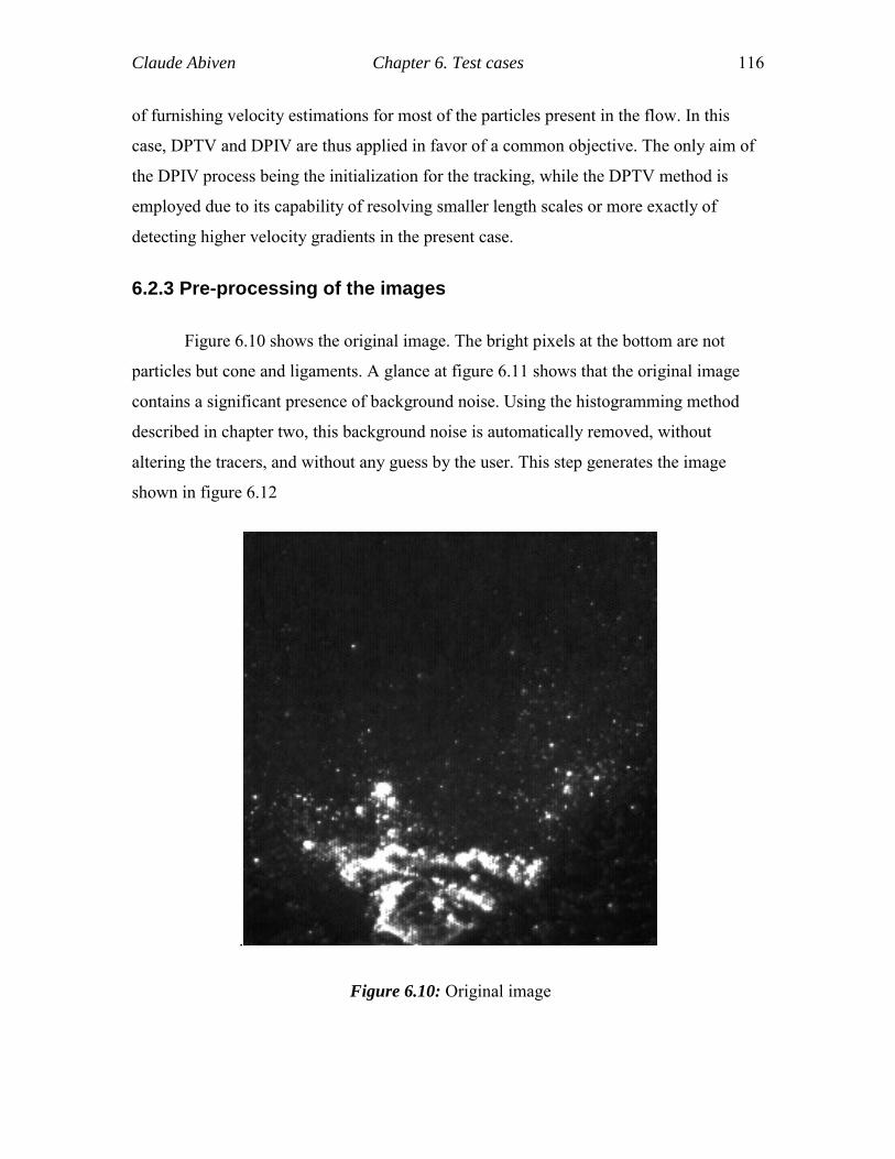
Claude Abiven Chapter 6. Test cases 116
of furnishing velocity estimations for most of the particles present in the flow. In this
case, DPTV and DPIV are thus applied in favor of a common objective. The only aim of
the DPIV process being the initialization for the tracking, while the DPTV method is
employed due to its capability of resolving smaller length scales or more exactly of
detecting higher velocity gradients in the present case.
6.2.3 Pre-processing of the images
Figure 6.10 shows the original image. The bright pixels at the bottom are not
particles but cone and ligaments. A glance at figure 6.11 shows that the original image
contains a significant presence of background noise. Using the histogramming method
described in chapter two, this background noise is automatically removed, without
altering the tracers, and without any guess by the user. This step generates the image
shown in figure 6.12
.
Figure 6.10: Original image
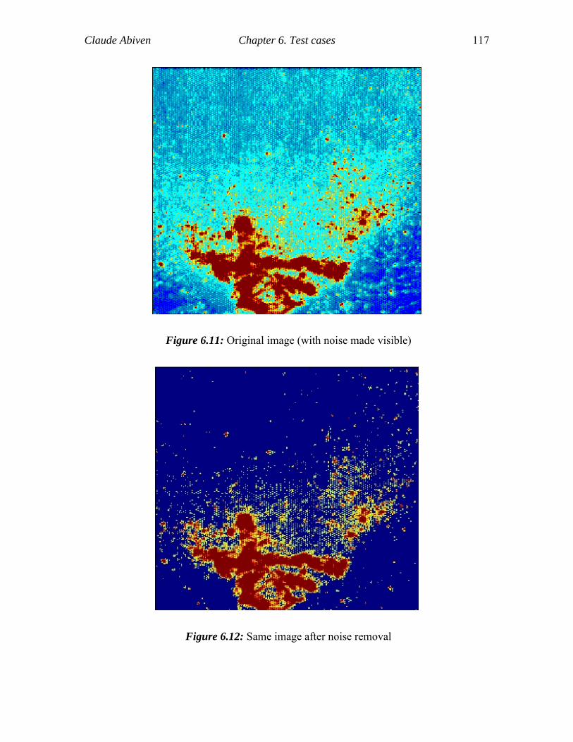
Claude Abiven Chapter 6. Test cases 117
Figure 6.11: Original image (with noise made visible)
Figure 6.12: Same image after noise removal
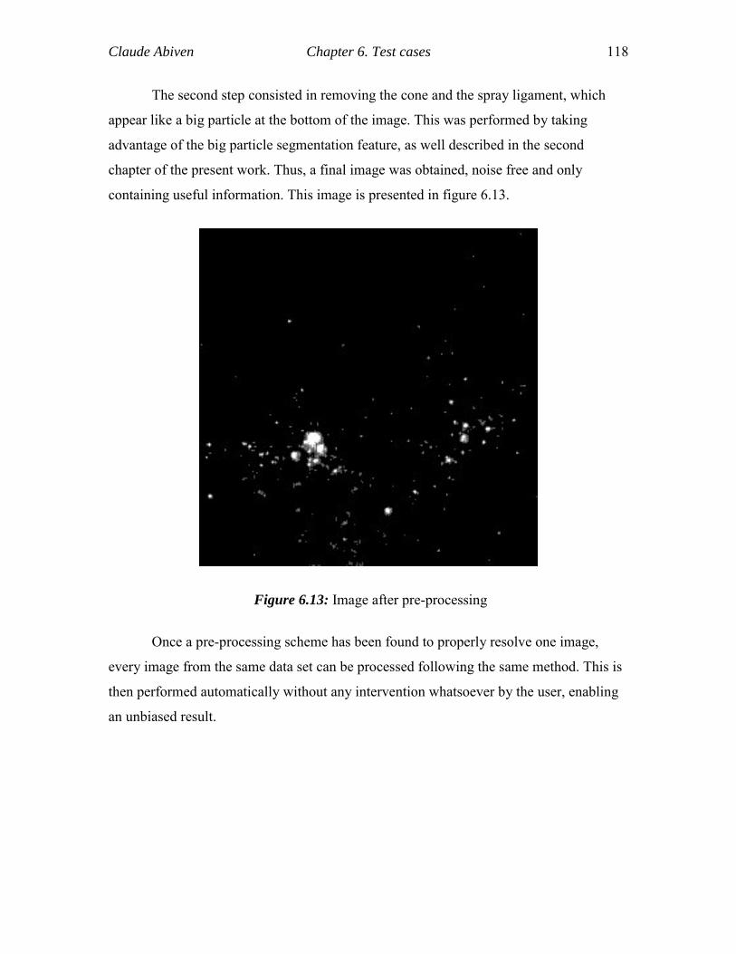
Claude Abiven Chapter 6. Test cases 118
The second step consisted in removing the cone and the spray ligament, which
appear like a big particle at the bottom of the image. This was performed by taking
advantage of the big particle segmentation feature, as well described in the second
chapter of the present work. Thus, a final image was obtained, noise free and only
containing useful information. This image is presented in figure 6.13.
Figure 6.13: Image after pre-processing
Once a pre-processing scheme has been found to properly resolve one image,
every image from the same data set can be processed following the same method. This is
then performed automatically without any intervention whatsoever by the user, enabling
an unbiased result.
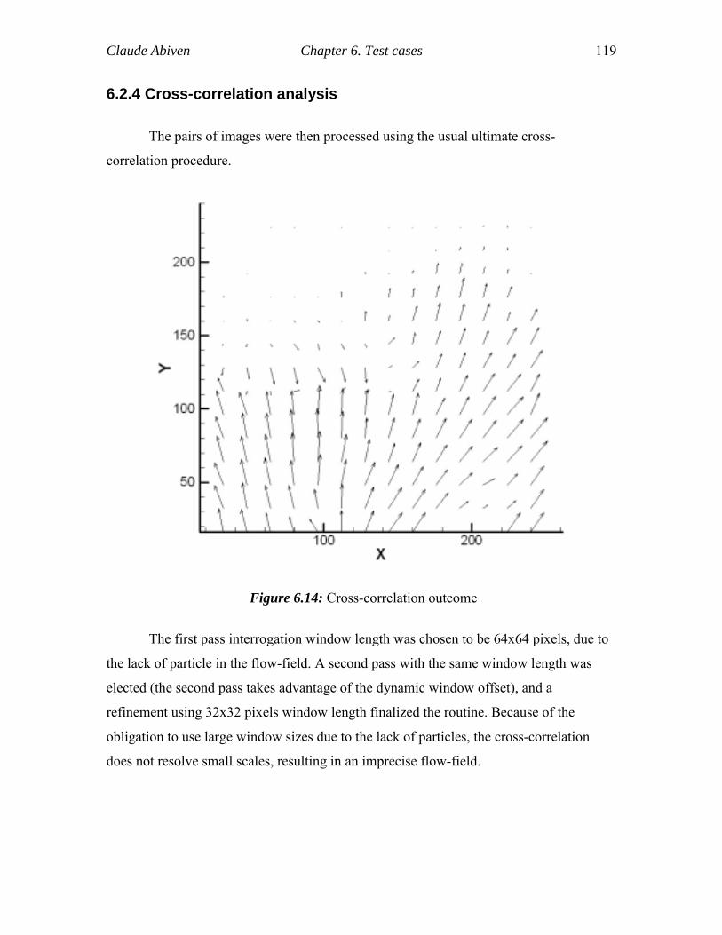
Claude Abiven Chapter 6. Test cases 119
6.2.4 Cross-correlation analysis
The pairs of images were then processed using the usual ultimate cross-
correlation procedure.
Figure 6.14: Cross-correlation outcome
The first pass interrogation window length was chosen to be 64x64 pixels, due to
the lack of particle in the flow-field. A second pass with the same window length was
elected (the second pass takes advantage of the dynamic window offset), and a
refinement using 32x32 pixels window length finalized the routine. Because of the
obligation to use large window sizes due to the lack of particles, the cross-correlation
does not resolve small scales, resulting in an imprecise flow-field.
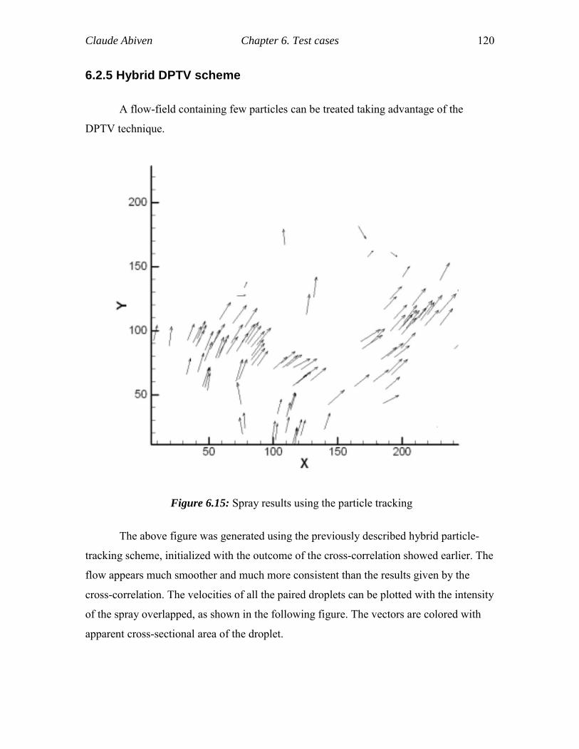
Claude Abiven Chapter 6. Test cases 120
6.2.5 Hybrid DPTV scheme
A flow-field containing few particles can be treated taking advantage of the
DPTV technique.
Figure 6.15: Spray results using the particle tracking
The above figure was generated using the previously described hybrid particle-
tracking scheme, initialized with the outcome of the cross-correlation showed earlier. The
flow appears much smoother and much more consistent than the results given by the
cross-correlation. The velocities of all the paired droplets can be plotted with the intensity
of the spray overlapped, as shown in the following figure. The vectors are colored with
apparent cross-sectional area of the droplet.
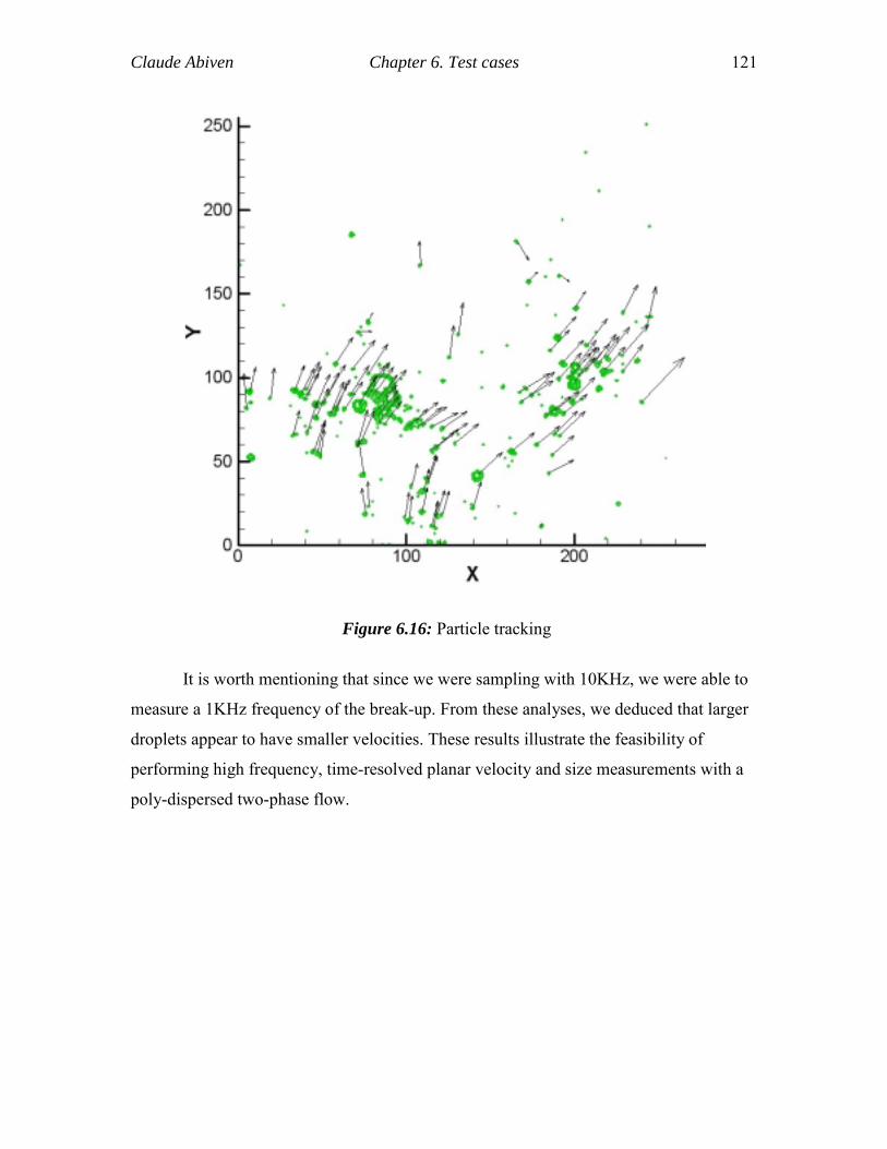
Claude Abiven Chapter 6. Test cases 121
Figure 6.16: Particle tracking
It is worth mentioning that since we were sampling with 10KHz, we were able to
measure a 1KHz frequency of the break-up. From these analyses, we deduced that larger
droplets appear to have smaller velocities. These results illustrate the feasibility of
performing high frequency, time-resolved planar velocity and size measurements with a
poly-dispersed two-phase flow.
122
Chapter 7 Conclusions and future work
7.1 Conclusions
Original methods in terms of Digital Particle Velocimetry and hybrid Particle
Tracking Velocimetry have been developed. A new way of implementing DPIV was
presented, providing flexibility, transparency, and accuracy to the method.
Starting from a very basic cross-correlation scheme, common features inherent to
usual DPIV schemes were implemented, including dynamic window offset and dynamic
adaptive windowing, as well as validation, interpolation and smoothing methods,
providing a robust and high-performing tool.
Significant improvements were brought to the method when incorporating an
arsenal of image-processing tools to the package, thus enabling multiphase-flows to be
computed by processing each phase independently. Additional features such as second
order offsets were successfully implemented. Moreover, the use of a neural network as a
post-processor for validating the cross-correlation outcome represented a considerable
advancement.
The major improvements that were discussed throughout this effort have effect at
the very core of the DPIV method, which happens to be critical for the global
performance of the system, reducing the number of stray vectors thus minimizing the
need of validation, data filtering and interpolation schemes. Any sort of interrogation
mesh can be generated, making possible to accurately resolve flows containing several
phases such as flows with droplets or bubbles. The use of a specific offset at each point of
the mesh was proved to provide much better accuracy in addition to limiting the effect of
an incorrect offset evaluation. Moreover, a solution was proposed in order to resolve this
last issue.
Claude Abiven Chapter 7. Conclusions and future work 123
A Hybrid DPTV system was also developed, including standard tracking routines,
as well as a cross-correlation-based scheme that enables hybrid Digital Particle Tracking
Velocimetry to take place without any interpolation. Using CMOS camera technology, an
innovative way of computing particles centroids has been demonstrated, making it
possible to determine the centroid of a particle even when in presence of saturated pixels.
In addition, using image processing along with a maximum intensity filter, particle
identification was made much more precise, enabling one to distinguish clustered
particles that an ordinary scheme would not distinguish.
These schemes have been successfully validated by statistical analyses proving
that they reach the best levels in DPIV standards. The ability of the method to resolve
multi-phase flows a well as challenging high-speed cavitating flows has also been
demonstrated.
7.2 Future work
Concerning the cross-correlation, two major points of interest have been
identified throughout the completion of this effort: reducing the peak-locking effect, and
improving the resolution of multiple length scales in a same flow-field. Although the
methods discussed in the present effort tackle this issue, enhancements might be
promising in this area.
The first problem might be treated by the completion of a “real offset” instead of
an “integer offset”. Indeed, since the smallest scale used in digital imaging is the pixel, it
doesn’t seem conceivable to shift an image by a non-integer number of pixels. However,
using image re-sampling, it might be possible to do so. The issue is to know if the error
introduced by re-sampling the image would be smaller than the error originated by
shifting a pixel to the nearest integer instead of the real corresponding displacement.
However, if it happened to be so, the peak-locking effect might be alleviated, and at the
same time, the overall error would considerably drop.
In order to resolve multiple length scales, it might be useful to try automatically
different window sizes in order to define the window offset correctly. Two ways might be

Claude Abiven Chapter 7. Conclusions and future work 124
considered. The first and more straightforward way was presented in the scope of this
work, but still needs further research and improvement: after having determined the
offset from a first pass, the result of the second pass is validated only if the resulting
displacement is found to be smaller than one pixel as it should. The second approach
would be to compare the cross-correlation peak as an indicator of the success of the
cross-correlation.
Regarding the particle tracking, the principal issues at stake remain the particle
identification together with the centroid location. An enhancement in the definition of
close particles would significantly improve the method.
125
References
1) Adrian RJ, Yao C-S (1985): Pulsed laser technique application to liquid and gaseous
flows and the scattering power of seed materials. App Optics, 24, 44-52.
2) Adrian RJ (1991): Particle-Imaging techniques for experimental fluid mechanics.
ARFM, 23, 261-304.
3) Adrian RJ, Meinhart CD, Barnhart DH and Papen GC (1995): An HPIV System for
turbulence research. EP Rood (ed.), ASME FED, 148,17-21.
4) Adrian RJ (1996): Bibliography of Particle Velocimetry using imaging methods. TAM
Report. Produced and distributed in cooperation with TSI Inc.
5) Adrian, R. J. (1996): Strategies for Imaging Flow Fields with PIV. AIAA 96-1988
6) Adrian, R. J. (1997): Dynamic Ranges of Velocity and Spatial Resolution of Particle
Image Velocimetry. Meas. Sci. Technol. 8 1393-1398.
7) Agui J. and Jimenez J. (1987): On the performance of particle tracking. J. Of Fluid
Mechanics vol 185 pp 447-468
8) Asimopoulos N, Vlachos P. P. Telionis D. P (1999): A high speed, high particle
density particle tracking method for turbulent flows. ASME FEDSM’99-7139.
9) Boedec T, Simoens S (2001): Instantaneous and simultaneous planar velocity field
measurements of two phases for turbulent mixing of high pressure sprays. Experiments
in Fluids, 31, 506-518.
10) Boillot A. and Prasad K. (1996): Optimization procedure for pulse separation in cross-
correlation PIV. Exp. In Fluids 21 87-93, Springer Verlag.
11) Carosone F. & A. Cenedese (1996): Image Analysis for velocity evaluation and Neural
Networks. VKI Lecture Series 1996-03
12) Cenedece A. Paglialunga A. (1990): Digital direct analysis of a multi-exposed
photograph in PIV. Exp. in Fluids 8, 273-280.
.
Claude Abiven References 126
13) Cowen B and Monismith S (1997): A hybrid digital particle tracking velocimetry
technique. Experiments in Fluids, 22, 199-211
14) Dalziel SB (1993): Decay of rotating turbulence: Some particle tracking experiments.
FTM Nieuwstadt (ed.). Flow Visualization and Image Analysis, 27-54
15) Damaschke N, Nobach H, Tropea C (2002): Optical limits of particle concentration for
multi-dimensional particle sizing techniques in fluids mechanics. Experiments in fluids,
32, 143-152.
16) Derou & Herault (1994): A new paradigm for particle tracking velocimetry based on
graph theory and pulsed neural networks. 7th Int. Symp. Appl. Laser Techniques to
Fluid Mechanics, Lisbon, pp: 35.3.1-35.3.8
17) Dracos Th. and A. Gruen (1998): Videogrammetric methods in velocimetry. Appl.
Mech. Rev. vol. 51, no. 6 1998
18) Grant I (1997): Particle Image Velocimetry: A Review. Proceedings Institute of
Mechanical Engineers
19) Grant and Pan (1995): An Investigation of the performance of multi layer neural
networks applied to the analysis of PIV images. Experiments in Fluids, pp 159-166.
20) Grant I (1994): Selected papers on Particle Image Velocimetry. SPIE Milestone Series
MS99, SPIE Optical Engineering Press, Bellingham, Washington
21) Guezennec YG and Kiritsis N (1990): Statistical investigation of errors in particle
image velocimetry. Experiments in Fluids, 10, 138-146.
22) Hammache M. & Gharib M. (1991): An experimental study of the parallel and oblique
vortex shedding from circular cylinders. J. Fluid Mech., vol. 232 pp. 567-590
23) Hasselinc L. (1988): Digital Image Processing in Flow Visualization. ARFM 20:421 85
24) Huang H. T. and Gharib M. (1997): Processing Error in Digital Particle Image
Velocimetry. FEDSM97-3068.
25) Huang, H. T. D. Dabiri and Gharib, M. (1997): On Errors of digital particle image
velocimetry. Meas. Science and Technology, .8, 1427-1440.
Claude Abiven References 127
26) Jahne B. (1991): Lectures in Computer Science. Spatio-Temporal Image Processing.
Springer-Verlag.
27) Jahne B. (1997): Image Processing for Scientific Applications. CRC Press
28) Keane R. D. and Adrian R. J. (1990): Optimization of particle image velocimeters .
Part I: Double pulsed systems. Meas. Sci. Tech. 1 1202-1205.
29) Keane R. D. and Adrian R. J. (1991): Optimization of particle image velocimeters .
Part I: Multiple pulsed systems. Meas. Sci. Tech. 2 963-974.
30) Khalitov DA, Longmire EK (2002): Simultanous two-phase PIV by two-parameter
phase discrimination. Experiments in Fluids, 32, 252-268.
31) Lecordier B and Trinite M (1999): Time resolved PIV measurements for high speed
flows. Third International Workshop on Particle Image Velocimetry. (Santa Barbara,
16-18 Sept 1999).
32) Lourenco L.M. (1996): Particle Image Velocimetry, Von Karman Institute Lecture
Series, 1996-03.
33) Meynard R. (1983): Measure de champs de vitesse d’ ecoulements fluids par analyse
de suites d’images obteneues par diffusion d’un fueillet lumineux. Ph.D Dissertation,
Faculte des Science Appliquees, Universite Libre de Bruxelles.
34) Mostafa, N., Nayfeh, A. H., Vlachos, P. P., and Telionis, D. P. (2001): Cavitating flow
over a projectile. AIAA 39th Aerospace Sciences Meeting and Exhibit, Reno, NV.
35) Prasad A. K. Adrian R. J., Landreth C.C., Offutt P.W.:(1992): Effect of resolution and
accuracy of particle image velocimetry interrogation. Exp. In Fluids 13 105-116,
Springer Verlag.
36) Prasad A.K. and Adrian R J (1993): Stereoscopic particle image velocimetry applied to
liquid flows. Experiments in Fluids 15, 49-60.
37) Press, Teukolsky, Vetterling, Flannery. (1992): Numerical Recipes in C: The Art of
Scientific Computing, Second Edition. Cambridge University Press.
38) Raffel M., Willert C.E. and Kompenhans J. (1998): Particle Image Velocimetry: A
practical guide. Series in Experimental Fluid Mechanics. Springer Verlag.
Claude Abiven References 128
39) RJ Perkings and JCR Hunt (1989): Particle Tracking in Turbulent Flows. Advances in
Turbulence 2 pp. 286-291.
40) Robinson O. Rockwell D. (1993): Construction of three-dimensional images of flow
structure via particle tracking techniques. Experiments in Fluids 14, 257-270
41) Scarano F. Rieuthmuller M.L. (1999): Iterative multigrid approach in PIV image
processing with discrete window offset. Exp. In Fluids 26 513-523, Springer-Verlag.
42) Upatnieks A., Laberteaux K., Ceccio S. L. (2002):A kilohertz frame rate
cinematographic PIV system for laboratory-scale turbulent and unsteady flows.
Experiments in Fluids, 32, 87-98.
43) Utami T. and Ueno T.(1984): Visualization and picture processing of turbulent flow.
Experiments in Fluids 2, 25-32, Springer-Verlag.
44) Vlachos P. P, Donnelly M. J. Telionis D. P. (1998): On the Wake of a Circular
Cylinder Piercing the Free-Surface. FEDSM’98-5177.
45) Vlachos, P. (2000): A spatio-temporal analysis of separated flows over bluff bodies
using quantitative flow visualization. PhD. Dissertation, Department of Engineering
Science and Mechanics, Virginia Polytechnic Institute and State University,
Blacksburg, VA.
46) Wereley ST, Meinhart CD (2001): Second-order accurate particle image velocimetry.
Experiments in Fluids, 31, 258-268.
47) Westerweel J (1997a): The effect of a discrete window offset on the accuracy of cross-
correlation analysis of digital PIV recordings. Exp. In Fluids 23 20-28, Springer
Verlag.
48) Westerweel J. (1993a): Digital Particle Image Velocimetry, Theory and Application.
Delft University Press
49) Westerweel J. (1993b):Optical Diagnostics in fluid and thermal flow. SPIE 2005 624-
35
50) Westerweel J. (1997b): Fundamentals of Digital Particle Image Velocimetry. Meas.
Sci. Technol. 8 1379-1392.
Claude Abiven References 129
51) Whybrew A, Reeves M, Slagle RL, Boaler JJ, Baughan AK, Nicholls TR, Towers DP,
Tavender B, Buckberry CH (1999): Two techniques for all-digital time-resolved PIV.
Third International Workshop on Particle Image Velocimetry. (Santa Barbara, 16-18
Sept 1999)
52) Willert C E and M Gharib (1991): Digital Particle Image Velocimetry. Experiments in
Fluids 10, 181-193 1991
53) Wung T. S. and Tseng F. G. (1992): A color-coded particle tracking velocimeter with
application to natural convection. Experiments in Fluids 13, 217-223
54) Wung T.S (1997): Quantitative visualization of 2D and 3D flows using a color-coded
particle tracking velocimetry. Atlas of Visualization III edited by The Visualization
Society of Japan.
130
VITA
Claude Abiven was born in January 17, 1977, in Rennes, France. He earned an
Engineering degree from the National Polytechnic Institute of Grenoble, France, in July
2000. In the spring of 2000, he completed an internship as a research assistant in the
fluids mechanics laboratory of Virginia Tech. This experience led him to enroll in
Virginia Tech in the spring of 2001