A Hybrid, Coupled Approach for Modeling Charged Fluids from the Nanoto the Mesoscale

James Cheunga,c, Amalie L. Frischknechtb,c,∗, Mauro Peregoa,c, Pavel Bocheva,c,∗

aCenter for Computing ResearchbCenter for Integrated Nanotechnologies

cSandia National Laboratories, Albuquerque, NM 87185, USA

Abstract

We develop and demonstrate a new, hybrid simulation approach for charged fluids, which combines the

accuracy of the nonlocal, classical density functional theory (cDFT) with the efficiency of the Poisson-

Nernst-Planck (PNP) equations. The approach is motivated by the fact that the more accurate description

of the physics in the cDFT model is required only near the charged surfaces, while away from these regions the

PNP equations provide an acceptable representation of the ionic system. We formulate the hybrid approach

in two stages. The first stage defines a coupled hybrid model in which the PNP and cDFT equations act

independently on two overlapping domains, subject to suitable interface coupling conditions. At the second

stage we apply the principles of the alternating Schwartz method to the hybrid model by using the interface

conditions to define the appropriate boundary conditions and volume constraints exchanged between the

PNP and the cDFT subdomains. Numerical examples with two representative examples of ionic systems

demonstrate the numerical properties of the method and its potential to reduce the computational cost of a

full cDFT calculation, while retaining the accuracy of the latter near the charged surfaces.

Keywords: Charged fluids, hard sphere model, PNP, classical density functional theory, Alternating

Schwartz method.

1. Introduction

Predictive simulations of steady-state flows of ionic solutions are important for a variety of techno-

logical applications, including flow through microfluidic and nanofluidic devices [1, 2], and flow through

ion-separation membranes [3]. These systems possess an electric double layer near surfaces, whose thickness

depends on ion concentration and surface charge, but is typically in the range of 1–10 nm. Devices of inter-

est, by contrast, can have dimensions ranging from tens of nm up to microns or larger. These devices often

operate in a regime where the details of the electric double layer near surfaces are important to the physics

and cannot be neglected. The latter makes the accurate modeling and simulation of these devises and the

∗Corresponding authorsEmail addresses: jcheung@sandia.gov (James Cheung), alfrisc@sandia.gov (Amalie Frischknecht), mperego@sandia.gov

(Mauro Perego), pbboche@sandia.gov (Pavel Bochev)

Preprint submitted to Elsevier January 3, 2017

associated ionic systems a challenging multiscale problem.

Steady-state flow and ion spatial distributions are typically calculated using the Poisson-Nernst-Planck

(PNP) model [4]. The PNP model comprises a set of Partial Differential Equations (PDEs) derived under

several simplifying assumptions about the ionic system. In particular, this model assumes that the ions

can be represented as point charges and that their spatial distribution is given by a simple Boltzmann

distribution determined by the electrostatic potential. The ionic solution is assumed to be ideal, with no

nonideal contributions to the chemical potential. The steady-state flux is determined by mass conservation.

However, in many practically important situations the PNP model is not adequate because the underlying

assumptions do not hold. Examples include ionic systems with high surface charge, multivalent ions, and

high ion concentrations. In such systems, the correlations between ions due to their finite size and due to

electrostatic correlations become important and must be properly accounted for by the model.

An attractive method for including these ion correlation effects is classical density functional theory

(cDFT). cDFT is a nonlocal theory for inhomogeneous fluids [5]. It is based on a variational principle and

is derived by minimizing the grand potential free energy of the system. cDFT has been shown to be highly

accurate for electrolyte solutions near charged surfaces, by comparison to both experiments and to particle-

based computer simulations such as Monte Carlo and molecular dynamics simulations [6, 7, 8]. For instance,

previous work by Gillespie and coworkers [8, 9] has shown that cDFT leads to significantly different results

than PNP for electrokinetic transport through uniform nanochannels, and that it can predict nonlinear

phenomena such as charge inversion that are seen experimentally [10].

Although cDFT is more computationally efficient than full particle simulations, it remains significantly

more expensive than PNP calculations. Because the effects described by cDFT are primarily important near

the surfaces, a hybrid model combining the detailed physics of cDFT in these regions with the computational

efficiency of PDEs away from them could be an effective way of modeling multiscale ionic systems.

Such hybrid multiscale approaches are attracting significant attention because, despite the continuing

advances in high-performance computing, monolithic microscopic or mesoscopic simulations of realistic prob-

lems remain out of reach. Most of the existing hybrid methods fall into one of the following three broad

categories. Blending or morphing approaches [11] use tools such as partition of unity to merge together

different mathematical models of the same physical phenomena. The latter can be accomplished in multiple

ways by blending, e.g., the energy, the force, or the material properties in the models. Examples of the

former include the Arleqiun scheme [12] and the energy-based blended quasicontinuum method [13], while

[14] is an instance of a force-based blended method. For examples of “morphing” methods, which blend

material properties we refer to [15, 16].

Optimization-based heterogeneous domain decomposition methods recast the coupling of the models

into a constrained optimization problem in which the objective is defined by a suitable coupling condition

and the models serve as the optimization constraints. The optimization-based local-to-nonlocal [17, 18]

and atomistic-to-continuum [19, 20] methods are examples of this approach, as is the optimization-based

2

multiscale method of [21].

Finally, classical overlapping and non-overlapping domain decomposition (DD) ideas [22] have also been

extended to the coupling of heterogeneous mathematical models. Examples include atomistic-to-continuum

coupling [23] and the coupling of continuum hydrodynamics and fluctuating hydrodynamics equations in

[24, 25].

The main goal of this work is to develop a hybrid method for ionic systems that combines the cDFT and

PNP models in a minimally intrusive way, so as to facilitate the reuse of existing simulation tools. A key

reason for this goal is our desire to leverage Sandia’s investments in the Tramonto code which implements

cDFT, and enable its coupling to a finite element code for the PNP model. Although both blending and

optimization-based methods have been successfully applied in multiple contexts, they are not the most

appropriate tool for this purpose as they require either significant modifications or additional capabilities

that may not be available in legacy codes. For instance, a blending method would require access to core

parts of the codes computing the energy, force or the material property, while an optimization-based method

depends on the availability of adjoints to solve the optimization problem.

In light of this, an overlapping domain decomposition framework such as the alternating Schwarz method

offers a particularly attractive setting for our purposes as it only requires exchange of boundary data between

the models. Consequently, we adopt this framework as a basis for the development of our hybrid cDFT-PNP

scheme. Preliminary numerical studies with the new hybrid model indicate that it is capable of correctly

capturing the physics of the double layer near the surfaces and blending it with the less detailed PNP solution

in the interior in a way that makes the hybrid simulation almost indistinguishable from a monolithic cDFT

simulation. At the same time, compared to the latter, the hybrid scheme allows for a significant reduction

in computational costs and memory usage.

We have organized the paper as follows. Section 2 summarizes the mathematical models of charged fluids

relevant to this paper and the associated physical systems that we target. In particular, we extend cDFT

modeling to non-uniformly charged nanochannels, in which the ion density profiles vary both across and

along the nanochannel. Section 3 presents our hybrid modeling approach. It starts with a simple numerical

example which motivates and illustrates the key idea of the strategy. We then proceed to define a coupled

hybrid cDFT–PNP model for charged fluids, which is then used to guide the development of a modified

Schwarz alternating procedure for such ionic systems. Finally, in Section 4 we use the new hybrid cDFT-

PNP approach to simulate steady-state ion transport through nanochannels. Our numerical results confirm

that the hybrid multiscale approach developed in this paper leads to considerable memory and computational

savings while preserving the detailed physics contained in the cDFT.

3

2. Mathematical Models

Consider a steady state charged fluid system comprising a mixture of N different ionic species α, α =

1, . . . , N , suspended in a solvent with a relative permittivity1 ε. In this paper we develop a hybrid simulation

approach for such systems, which combines two mathematical models having different levels of physical

fidelity. Both models describe the ionic species α by means of their concentrations (densities) ρα, and share

a common mathematical structure comprising a Poisson equation

−∇2φ(r) =q(r)

εε0(1)

for the electrostatic potential φ(r) and a set of N conservation laws

∇ · Jα = 0, α = 1, . . . , N (2)

for the flux of each ionic species. The latter follow from the fact that in steady state flows the mass is

conserved and so the total ion flux through the boundary of any volume is zero. To close the system (1)–(2)

we express the total charge density q(r) and the flux Jα in terms of the ionic concentrations ρα. We define

the former according to

q(r) =∑α

ezαρα, (3)

where e is the elementary charge, and zα is the valence of the species α, while for the ionic flux we assume

the constitutive relation

Jα = −Dαρα∇(βµα), (4)

where Dα and µα are the diffusion constant and the chemical potential of species α, respectively, while

β =1

kT

with k being Boltzmann’s constant and T the temperature.

The differential equations (1)–(2), along with (3)–(4) represent a generic model for the steady state ionic

system. The two models comprising our hybrid scheme are specializations of this generic model corresponding

to two different ways of handling the ions. The less accurate but more efficient PNP model treats the ions

as ideal point charges, whereas the more accurate but less efficient cDFT model treats these particles as

hard spheres with possibly different diameters. Ultimately, these different ion descriptions lead to different

expressions for the associated chemical potentials µα but apart from that do not affect the structure of the

generic model (1)–(4). As a result, the distinctions between the PNP and the cDFT models remain confined

to the constitutive relation (4) for the flux, while the potential equation (1) and definition (3) for the total

charge remain unchanged. We discuss the specific forms of the chemical potentials for the PNP and cDFT

models, the resulting sets of governing equations, and the necessary boundary conditions in the following

sections.

1We denote the permittivity of free space by ε0 and use SI units.

4

2.1. The steady-state PNP model

Under the PNP assumption that the ions are ideal, point charges, the chemical potentials can be expressed

directly in terms of the densities ρα and the electric potential φ as follows:

µPNPα = β−1 ln ρα + ezαφ; α = 1, . . . , N. (5)

Substitution of (5) into the constitutive relation (4) results in the following expression for the flux of the

ionic species:

Jα = −Dα∇ρα − β Dαezαρα∇φ, α = 1, . . . , N. (6)

Finally, combining (6) with the conservation law (2) yields the steady-state Nernst-Planck equations

∇ · (Dα∇ρα + β Dαezαρα∇φ) = 0, α = 1, . . . , N (7)

for the ionic concentrations ρα, α = 1, . . . , N . Together with the potential equation (1), and the definition

(3) of the charge density, the Nernst-Planck equations (7) form a system of N+1 nonlinear partial differential

equations for the variables ρα and φ. This system is the Poisson-Nernst-Planck (PNP) model of our charged

fluid system.

Boundary conditions. The well-posedness of the PNP model (1), (3), and (7) requires the specification of

suitable boundary conditions for the potential and the ionic concentrations.

Let ∂n denote the normal derivative to the boundary Γ of the domain Ω containing the charged fluid.

For the electrostatic potential one can consider either Dirichlet or Neumann conditions, i.e., on Γ we specify

either

φ = φbd or ∂nφ = − qsεε0

(8)

where φbd is a given boundary electric potential and qs is a given surface charge.

The Nernst-Planck equations (7) can also be augmented by Dirichlet or Neumann boundary conditions.

In this work we restrict attention to the former, i.e., we specify

ρα = ρbdα . (9)

where ρbdα is a given boundary ionic concentration.

Length scales. The typical length scale associated with solutions to the PNP equations is the Debye length

κ, where

κ2 ≡ kTεε0∑α e

2z2αρ

bα

. (10)

This is the length scale at which the ion densities decay away from a charged surface. Another important

length scale is the Bjerrum length,

lB ≡e2

4πkTεε0, (11)

which is the length at which the electrostatic interactions have strength kT .

5

2.2. The steady-state non-equilibrium cDFT model

The idealization of the ions as point charges in the PNP model limits its physical fidelity. The non-

equilibrium semi-primitive cDFT model in this paper uses a more realistic representation of these particles

as charged hard spheres2 that can have different sizes. This assumption leads to a more accurate description

of the chemical potentials, which augments the PNP potential by correction terms accounting for the finite

size of the ions:

µcDFTα = µPNPα + Vα + β−1 δFhs

δραα = 1, . . . , N. (12)

The first correction term, Vα(r) is the neutral part of the external field due to the surfaces acting on each

site α. The second correction term is the Jacobian of the hard sphere contribution, given by [26, 27]

Fhs [ρα(r)] = β−1

∫drΦ, (13)

where Φ is the energy density for the hard sphere system. This energy density is a function of the scalar and

vector Rosenfeld nonlocal (weighted) densities, denoted by nγ , γ = 0, 1, 2, 3 and nν , ν = 1, 2, respectively,

and has the following form:

Φ = −n0 ln (1− n3) +n1n2 − n1 · n2

1− n3+(n3

2 − 3n2n2 · n2

) n3 + (1− n3)2 ln(1− n3)

36πn23(1− n3)2

. (14)

The nonlocal Rosenfeld densities are defined by

nγ(r) =∑α

∫dr′ ρα(r)ω(γ)

α (r− r′), and nν(r) =∑α

∫dr′ ρα(r)ω(ν)

α (r− r′), (15)

respectively, where ω(γ)α and ω

(ν)α are scalar and vector weighting functions. These weighting functions are

based on the geometric properties of the hard spheres and are given byω

(0)α (r) =

ω(2)α (r)

4πR2α

ω(1)α (r) =

ω(2)α (r)

4πRα

;ω

(2)α (r) = δ(Rα − |r|)

ω(3)α (r) = θ(Rα − |r|)

and

ω

(1)α (r) =

ω(2)α (r)

4πRα

ω(2)α (r) =

r

rδ(Rα − |r|)

,

respectively, where δ(r) and θ(r) denote the Dirac delta function and Heaviside step function, respectively,

and Rα is the radius of species α. The energy density used in this paper was designed to match the

Mansoori-Carnahan-Starling-Leland (MCSL) equation of state [29] for multi-component hard-sphere fluids.

Owing to the inclusion of the hard sphere terms (12) is a nonlocal integral equation. Thus, the steady-

state cDFT model is a system of integro-differential equations for the variables ρα, µα, and φ, comprising

the differential equations (1)–(2) from the generic model, along with (3)–(4), and the nonlocal equation (12)

for the chemical potential. This steady-state cDFT model was previously shown to be in good agreement

with grand canonical Monte Carlo simulations [30].

2The cDFT version used in this paper is based on the fundamental measure theory for hard spheres [26, 27, 28].

6

Boundary and volume constraints. Because the cDFT model involves local and nonlocal equations it requires

a combination of conventional boundary conditions and Dirichlet volume constraints. Since the part of the

cDFT model dealing with the electrostatic potential is the same as in the generic and PNP models, for this

variable we retain the boundary conditions in (8), i.e., we specify either Dirichlet or Neumann conditions for

φ. For the ion densities we consider the volume constraints

ρα = ρbulkα , α = 1, . . . , N,

also referred to as bulk constraints. Volume constraints are a generalization of Dirichlet boundary conditions

for nonlocal equations; see, e.g., [31] for further details. Finally, for the chemical potentials we prescribe the

Dirichlet conditions

µα = µbdα , (16)

where µbdα is given on the boundary of the domain.

2.3. PNP as a simplification of non-equilibrium cDFT

The expressions for the PNP and cDFT chemical potentials suggest that one can view the PNP model

as a simplification of the non-equilibrium cDFT. Indeed, assuming Vα = 0, the two potentials (5) and (12)

only differ by the non-ideal terms β−1δFhs/δρα, which vanish in the limit of point charges. Since a nonzero

Vα can be included into the PNP model by modifying the expression for Jα, it follows that in the point

charge limit the cDFT potential (12) reduces to the PNP potential (5), i.e., the non-equilibrium cDFT

model reduces to the PNP model. It should be noted though, that the addition of the excess Helmholtz free

potential significantly changes the model from both mathematical and numerical points of view, transforming

a system of PDE equations into a system of integro-differential equations.

2.4. Application Problems

This section describes two example problems used to test and demonstrate the proposed hybrid cDFT-

PNP approach. To define these problems we choose model parameters consistent with aqueous ionic solutions.

Specifically, the temperature is T = 298K, the background fluid dielectric permittivity is ε = 78.5, and the

ions are assumed to have a diameter of λ = 0.3 nm, which is typical of hydrated ions. In Example 2 below,

we consider ions of different sizes, with the cations of diameter 1λ and the anions of diameter 1.5λ. With

these parameters, the Bjerrum length lB = 7.14 A. As explained in Section 2.2, for the cDFT model we

treat the ionic solutions using the semi-primitive model, in which all species are hard spheres. The ions are

charged, while the solvent is either represented by a neutral hard sphere or as a continuum background.

In this section, for simplicity, lengths, densities, the electrostatic potential, chemical potentials and

external fields are in dimensionless units, without changing notation. Characteristic units are: λ for lengths,

λ−3 for site densities, e/kT for the electrostatic potential and kT for chemical potentials and external fields.

We vary ion concentrations from 10 mM to 1 M, which in nondimensionless units is from 0.00016 to 0.016.

For simplicity we take the diffusion constants to be Dα = 1.

7

Example problem 1. Many technologies, ranging from water filtration to electrochemical devices such as

fuel cells, involve ion transport across selective, porous membranes. Predictive simulation of such transport

processes requires more accurate description of the physics than that afforded by the PNP model [32, 3].

Our first example problem captures the essential characteristics of the ion transport in a simplified one-

dimensional setting and is intended to demonstrate the potential of the hybrid approach for this type of

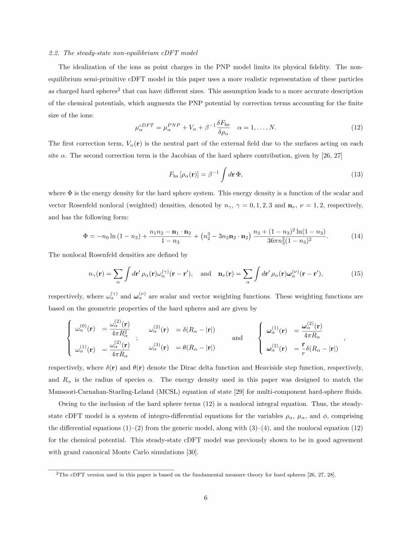
application. In this example we consider diffusion across a charged, semi-permeable planar membrane with

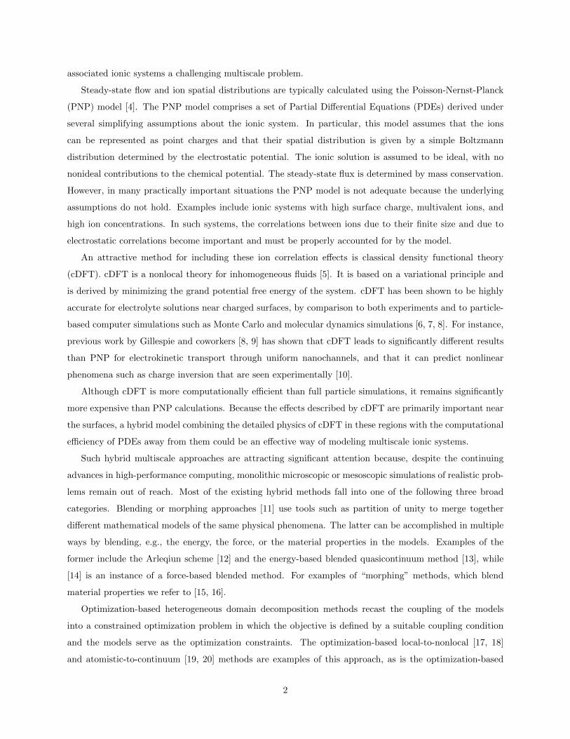
thickness 10d ≈ 3 nm; see Figure 1. We assume that all dependent variables vary only in a direction x

perpendicular to the membrane, and that the membrane extends from xl to xr in that direction. The

ionic system is a three component fluid with cations, anions, and a neutral solvent, with densities ρ+(x),

ρ−(x), and ρ0(x), respectively. The membrane interacts with the fluid species through a simple square-well

potential:

Vα(x) =

εα, xl < x < xr

0, x ≤ xl, x ≥ xr. (17)

The membrane is repulsive to the cations and the neutral fluid, with εc = εs = 2.0, and attractive to

the anions with εa = −2.0. The membrane is slightly positively charged, with charge density 0.01e/λ2.

In this problem we apply both a concentration gradient and an electrostatic potential gradient across the

membrane.

Figure 1: Diagram of 1D channel. Shaded regions represent the left and right reservoirs and the semi-permeable membrane in

the middle. The membrane extends from xl = 55 to xr = 65. The values in the gray shaded areas specify the bulk densities

and the potential gradient for the numerical study in Section 4.1.

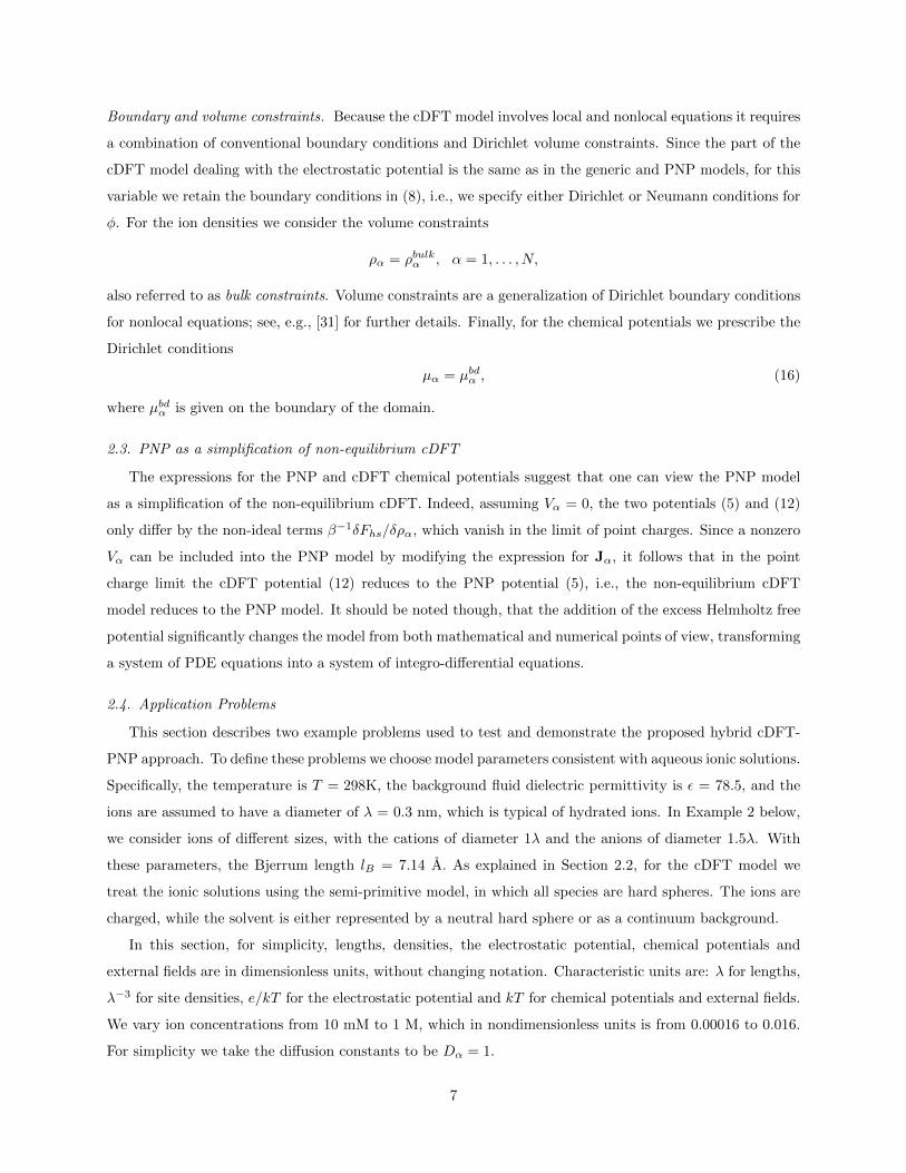
Example problem 2. We consider steady-state ion transport through a nanochannel with inhomogeneously

charged channel walls. This example is motivated by experiments and prior studies of nanofluidic devices

that act as diodes [33, 34, 35, 36, 37]. The current through such devices is significantly larger for a potential

bias applied in one direction, a phenomenon known as current rectification. In particular, Karnik et al. [34]

fabricated rectangular nanochannels of height 30 nm, in which half the channel carried a positive surface

charge density while the other half had neutral (or near neutral) surfaces [34]. This experimental work

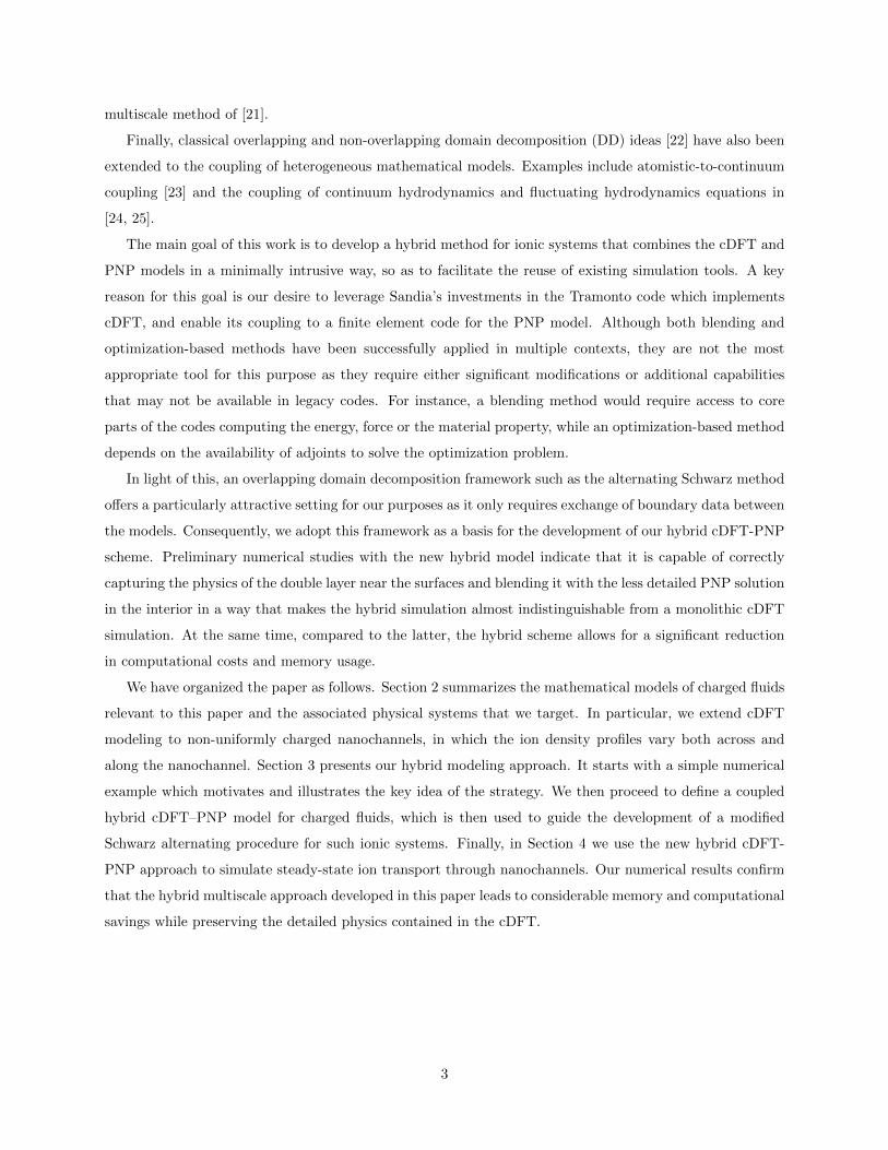
motivates our choice of the nanochannel geometry shown in Fig. 2. The channel occupies the middle of the

domain, with a reflective boundary at the channel’s axis for computational convenience. This allows us to

model only half of the device. There are two reservoir regions on either side of the nanochannel. On the

two ends of the channel, the chemical potentials µ in the cDFT calculations are held constant in a small

8

region to model the bulk reservoir fluid. We recall that this volume constraint is an analogue of the Dirichlet

boundary conditions in PDEs. The channel wall is negatively charged on the left side of the channel and

is neutral on the right side. All variables in this problem intrinsically vary in both the x and y directions,

leading to a 2D problem; we assume the system is uniform in the z direction.

Figure 2: Diagram of 2D nanochannel, showing reservoirs and the charged wall.

3. The Hybrid cDFT–PNP Coupled Model and its iterative solution

This section presents our hybrid cDFT-PNP coupling strategy. At the core of this strategy is the ob-

servation that, for a range of application problems, the cDFT and PNP models are in good agreement in

those regions that are away from the charged surfaces. Thus, a more cost-effective alternative to a full cDFT

simulation would be to use this more accurate, but more expensive model only near the charged surfaces

and then switch to the less accurate but more efficient PNP model away from these surfaces.

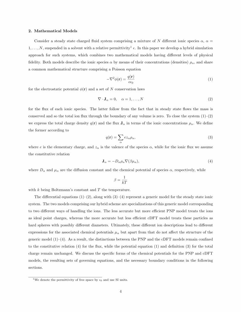
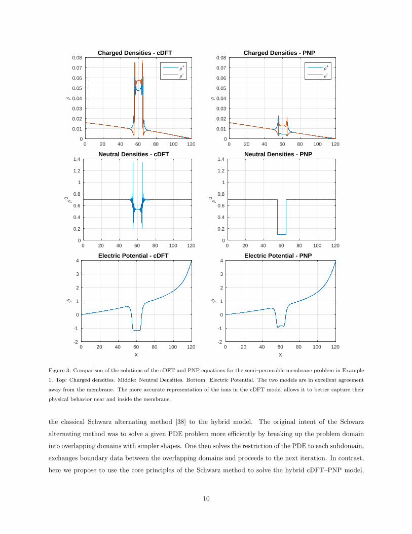
To lend further credence to this strategy, in Figure 3 we compare the cDFT and PNP solutions for the 1D

semi-permeable membrane problem in Example 1. We see that far from the membrane, the PNP and cDFT

density profiles are smooth and essentially identical. However, both inside and near the semi-permeable

membrane the two models exhibit significant qualitative and quantitative differences. In particular, the

presence of the membrane causes some layering in the cDFT solution, due to packing effects among the

hard spheres. In contrast, the PNP solution does not develop a strong layering behavior and predicts much

lower ion densities in the membrane. The same observations hold true for the neutral density where the

PNP solution completely misses the layered behavior of this variable near and inside the membrane, but is

essentially identical to the cDFT solution away from the membrane.

To summarize, we suggest solving the cDFT problem only in the regions, close to charged walls, where

treating the ions as hard spheres is required to resolve the physics, and use the PNP model in the remaining

parts of the domain, where the idealization of the ions as point charges is completely adequate.

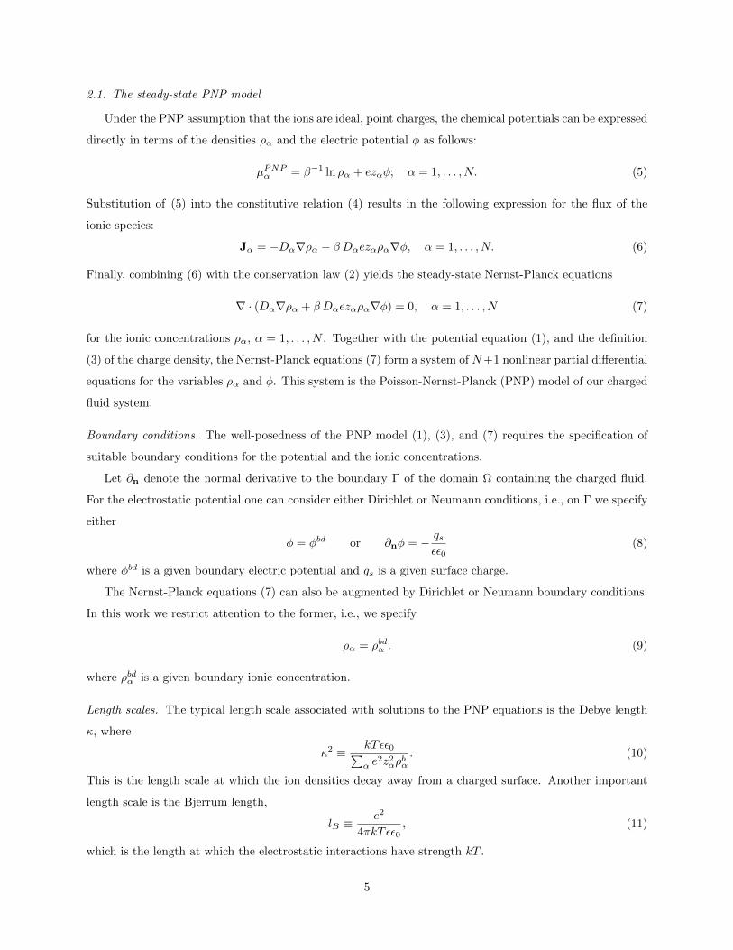
We implement this hybrid cDFT–PNP approach in two stages. In the first stage we formulate a coupled

cDFT–PNP model for charged fluids in which the cDFT and PNP equations operate on two separate but

overlapping domains; see Fig. 4. Specification of suitable transmission conditions on the interfaces engendered

by the overlap region couples the two sets of equations and completes the definition of the hybrid model.

At the second stage we develop an iterative procedure to solve this hybrid model. To this end, we extend

9

x0 20 40 60 80 100 120

;

0

0.01

0.02

0.03

0.04

0.05

0.06

0.07

0.08Charged Densities - cDFT

;+

;-

x0 20 40 60 80 100 120

;

0

0.01

0.02

0.03

0.04

0.05

0.06

0.07

0.08Charged Densities - PNP

;+

;-

x0 20 40 60 80 100 120

;0

0

0.2

0.4

0.6

0.8

1

1.2

1.4Neutral Densities - cDFT

x0 20 40 60 80 100 120

;0

0

0.2

0.4

0.6

0.8

1

1.2

1.4Neutral Densities - PNP

x0 20 40 60 80 100 120

?

-2

-1

0

1

2

3

4Electric Potential - cDFT

x0 20 40 60 80 100 120

?

-2

-1

0

1

2

3

4Electric Potential - PNP

Figure 3: Comparison of the solutions of the cDFT and PNP equations for the semi–permeable membrane problem in Example

1. Top: Charged densities. Middle: Neutral Densities. Bottom: Electric Potential. The two models are in excellent agreement

away from the membrane. The more accurate representation of the ions in the cDFT model allows it to better capture their

physical behavior near and inside the membrane.

the classical Schwarz alternating method [38] to the hybrid model. The original intent of the Schwarz

alternating method was to solve a given PDE problem more efficiently by breaking up the problem domain

into overlapping domains with simpler shapes. One then solves the restriction of the PDE to each subdomain,

exchanges boundary data between the overlapping domains and proceeds to the next iteration. In contrast,

here we propose to use the core principles of the Schwarz method to solve the hybrid cDFT–PNP model,

10

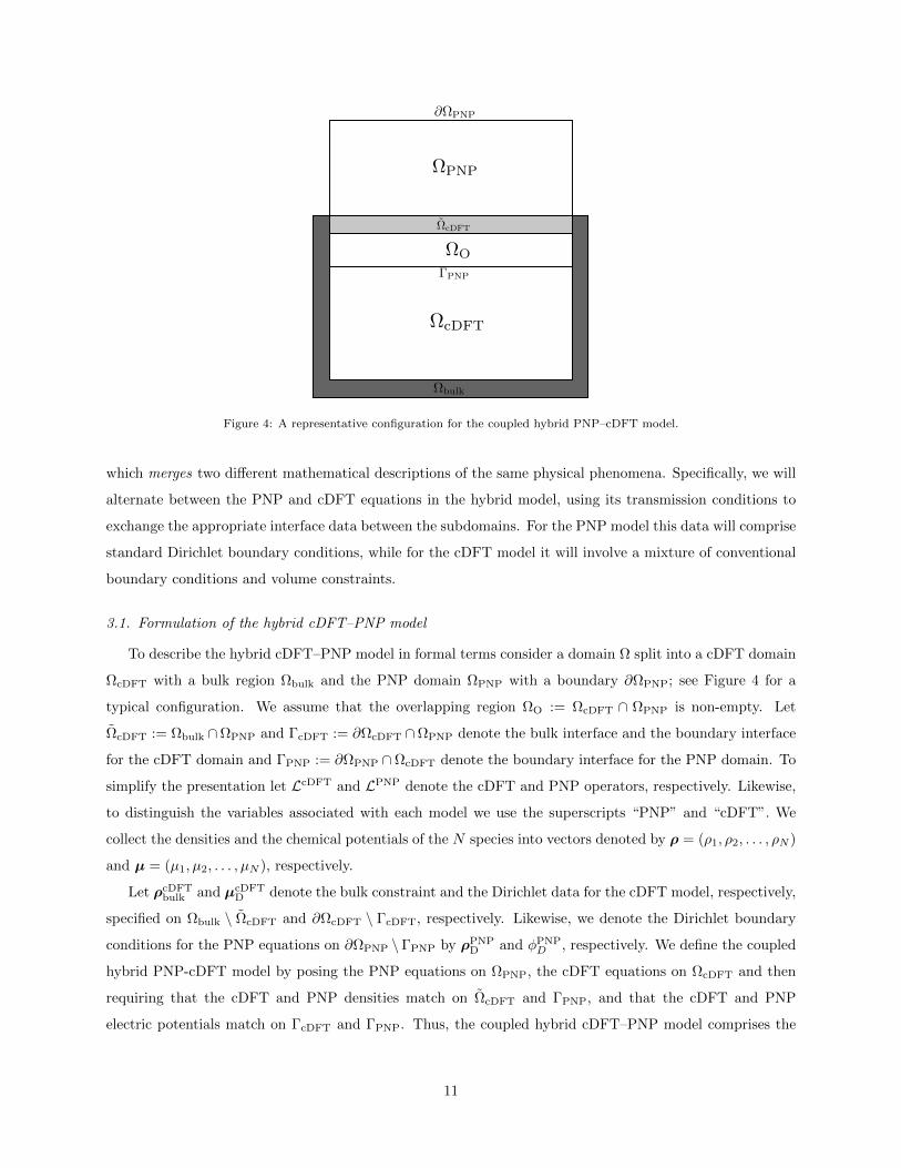
Figure 4: A representative configuration for the coupled hybrid PNP–cDFT model.

which merges two different mathematical descriptions of the same physical phenomena. Specifically, we will

alternate between the PNP and cDFT equations in the hybrid model, using its transmission conditions to

exchange the appropriate interface data between the subdomains. For the PNP model this data will comprise

standard Dirichlet boundary conditions, while for the cDFT model it will involve a mixture of conventional

boundary conditions and volume constraints.

3.1. Formulation of the hybrid cDFT–PNP model

To describe the hybrid cDFT–PNP model in formal terms consider a domain Ω split into a cDFT domain

ΩcDFT with a bulk region Ωbulk and the PNP domain ΩPNP with a boundary ∂ΩPNP; see Figure 4 for a

typical configuration. We assume that the overlapping region ΩO := ΩcDFT ∩ ΩPNP is non-empty. Let

ΩcDFT := Ωbulk ∩ΩPNP and ΓcDFT := ∂ΩcDFT ∩ΩPNP denote the bulk interface and the boundary interface

for the cDFT domain and ΓPNP := ∂ΩPNP ∩ΩcDFT denote the boundary interface for the PNP domain. To

simplify the presentation let LcDFT and LPNP denote the cDFT and PNP operators, respectively. Likewise,

to distinguish the variables associated with each model we use the superscripts “PNP” and “cDFT”. We

collect the densities and the chemical potentials of the N species into vectors denoted by ρ = (ρ1, ρ2, . . . , ρN )

and µ = (µ1, µ2, . . . , µN ), respectively.

Let ρcDFTbulk and µcDFT

D denote the bulk constraint and the Dirichlet data for the cDFT model, respectively,

specified on Ωbulk \ ΩcDFT and ∂ΩcDFT \ ΓcDFT, respectively. Likewise, we denote the Dirichlet boundary

conditions for the PNP equations on ∂ΩPNP \ΓPNP by ρPNPD and φPNP

D , respectively. We define the coupled

hybrid PNP-cDFT model by posing the PNP equations on ΩPNP, the cDFT equations on ΩcDFT and then

requiring that the cDFT and PNP densities match on ΩcDFT and ΓPNP, and that the cDFT and PNP

electric potentials match on ΓcDFT and ΓPNP. Thus, the coupled hybrid cDFT–PNP model comprises the

11

subdomain governing equations

LcDFT(ρcDFT, φcDFT,µcDFT) = 0 in ΩcDFT

ρcDFT = ρcDFTbulk on Ωbulk\ΩcDFT

φcDFT = φcDFTD on ∂ΩcDFT\ΓcDFT

µcDFT = µcDFTD on ∂ΩcDFT\ΓcDFT

;

LPNP(ρPNP, φPNP) = 0 in ΩPNP

ρPNP = ρPNPD on ∂ΩPNP\ΓPNP

φPNP = φPNPD on ∂ΩPNP\ΓPNP

(18)

along with the interface conditions:ρcDFT = ρPNP on ΩcDFT

φcDFT = φPNP on ΓcDFT

µcDFT = µ(ρPNP, φPNP) on ΓcDFT

and

ρPNP = ρcDFT on ΓPNP

φPNP = φcDFT on ΓPNP

, (19)

where

µα(ρPNPα , φPNP) := ln

(ρPNPα

)+ zαφ

PNP + V (x) +δFex

δρα(ρPNPα ) (20)

In the PNP model, the chemical potential is not an unknown because it depends algebraically on the densities

and the electric potential. Accordingly we prescribe boundary conditions only for the density and for the

electric potential. On the contrary, the chemical potential is an unknown in the cDFT model, i.e., it requires

an appropriate boundary condition on the interface. Given the PNP densities in the bulk region ΩcDFT and

the PNP electric potential on ΓcDFT, we recover the chemical potential µ on ΓcDFT using expression (20).

In what follows ucDFT = (ρcDFT, φcDFT) and uPNP = (ρPNP, φPNP) denote the solution vectors of the

cDFT and PNP models, respectively. We combine these solutions into a solution uhyb of the hybrid model

(18), according to

uhyb =

ucDFT if x ∈ ΩcDFT

uPNP if x ∈ ΩPNP \ ΩO.(21)

This definition of uhyb uses the more accurate cDFT solution in the overlap region ΩO.

3.2. Extension of the Schwarz alternating method to the hybrid model

In this section we extend the classical overlapping Schwarz method to the hybrid cDFT-PNP model

by applying the principles of the alternating Schwarz iteration to (18), (19), and (20). Recall that in the

classical setting the same models posed on overlapping domains exchange boundary data. Here we use the

interface conditions (19) to define the proper data exchange between the two different models in (18). This

yields the following generalized Schwarz alternating procedure for the solution of the coupled hybrid problem

12

(18)–(20):

Begin with initial guesses ρcDFT0 and φcDFT

0 on ΓPNP.

Set k = k + 1 and solve:

(PNP)

LPNP(ρPNP

k , φPNPk ) = 0 in ΩPNP

ρPNPk = ρcDFT

k−1 on ΓPNP

φPNPk = φcDFT

k−1 on ΓPNP

(cDFT)

LcDFT(ρcDFTk , φcDFT

k ,µcDFTk ) = 0 in ΩcDFT

ρcDFTk = ρPNP

k on ΩcDFT

φcDFTk = φPNP

k on ΓcDFT

µcDFTk = µ(ρPNP

k , φPNPk ) on ΓcDFT

If diff(uhybk ,uhyb

k+1) ≥ δ then continue; else: stop.

(22)

In (22) the symbol diff() stands for a function used to define the convergence criteria of the algorithm and

δ is a prescribed error tolerance value. Let

||u||L2(Ω) =

(∫Ω

φ2dx+

N∑α=1

∫Ω

ρ2αdx

) 12

.

denote the L2 norm of the hybrid solution. A standard choice for diff() is the relative difference of two

consecutive iterates, i.e.,

diff(uhybk ,uhyb

k+1) = Dhybrel (uhyb

k ,uhybk+1) :=

‖uhybk+1 − uhyb

k ‖L2(Ω)

‖uhybk+1‖L2(Ω)

(23)

We define the relative L2 error of the hybrid solution according to

Ehybrel :=

||uhyb − ucDFT||L2(Ω)

||ucDFT||L2(Ω). (24)

The relative error requires computation of the cDFT solution on all of Ω and so, it is not a practical

alternative to (23). We use (24) to quantify the modeling error of the hybrid formulation.

Remark 1. It is well-known that the convergence of the classical Schwarz alternating method for a linear

elliptic PDE depends on the size of the overlap region [38]. The same holds true for its generalization (22),

however, the size and the placement of the overlap domain ΩO in the present context is subject to additional

considerations. First, since the cDFT model requires a volume constraint, the size of the bulk region ΩcDFT

defines a strict lower bound for the size of ΩO. Second, as the results in Fig.3 suggest, ΩO must be placed at

a site where the nonlocal effects in the cDFT model are small. This should be contrasted with the classical

Schwarz method where the choice of the subdomains is governed by computational efficiency rather than

model behavior. We examine these issues numerically and provide some recommendations in Section 4.1.2.

13

Remark 2. In the classical application of the Schwarz method the initial guess is typically set to zero because

at this stage there’s no subdomain solution information available on the interfaces. In principle, one could

make the same choice in (22), i.e., set ρcDFT0 = 0 and φcDFT

0 = 0. However, taking into account that the

purpose of (22) is to merge two different models operating on different subdomains, rather than to solve

a single PDE more efficiently by breaking it up, a potentially better choice for the initialization emerges.

Specifically, according to Remark 1 the overlap domain must be chosen in such a way that the nonlocal

effects of the cDFT model become almost negligible. As a result, it is reasonable to expect that the cDFT

and PNP solutions will be close in this region and so, one can set the initial data by using a global solution

(ρPNPΩ , φPNP

Ω ) of the PNP model on all of Ω, i.e., ρcDFT0 = ρPNP

Ω

∣∣∣ΓPNP

and φcDFT0 = φPNP

Ω

∣∣∣ΓPNP

. We examine

this choice in Section 4.1.

3.3. Implementation of generalized Schwarz method for the hybrid model

The subdomain solutions of the cDFT–PNP hybrid model were computed using the cDFT and PNP

capabilities of the parallel, C++, open source package Tramonto3. Tramonto solves numerically the governing

equations in Rd, d = 1, 23 using a Cartesian mesh and piecewise linear/bilinear/trilinear finite elements.

The nonlinearity of the governing equations is handled by an inexact Newton’s method. The resulting

linear systems are solved using GMRES preconditioned with an algebraic multigrid preconditioner [39] (ML)

implemented in the Trilinos software suite [40]. For further details on the numerical methods and the

application of Tramonto for the simulation of charged systems we refer to [30, 41, 42, 43].

Our implementation of (22) uses two separate instances of Tramonto modified to accommodate the

requirements of the algorithm. Specifically, the PNP instance was modified to read in the required boundary

information from the cDFT iterate, while the cDFT instance was modified to read in the required boundary

and volume constraint information from the PNP iterate. In this work we used two instances of Tramonto

because it already contained a PNP implementation sufficient for our purposes. However, it should be clear

that the cDFT instance of Tramonto developed in this work can be paired with any available implementation

of the PNP model, as long as it can exchange the information required by (22).

4. Computational Results

Numerical results in this section illustrate computational properties of the generalized Schwarz procedure

(22) for the hybrid cDFT–PNP formulation (18), with a particular emphasis on its accuracy and efficacy.

For the former task, in Section 4.1, we restrict attention to one-dimensional examples as they are sufficient

to reveal key convergence and error behavior trends of (22). We also use the one dimensional setting to

investigate two different initialization strategies for (22), and how the size and the placement of the overlap

region affects the properties of (22). Characterization of the efficiency gains afforded by the hybrid approach

3See http://software.sandia.gov/tramonto.

14

requires a more challenging setting, though. In Section 4.2 we demonstrate the CPU time reduction and the

memory savings of (22) by using the two-dimensional setting of Example 2 together with cDFT and PNP

discretizations leading to large scale numerical simulations with millions of unknowns.

4.1. Iterative Convergence and Modeling Error

We use Example 1 in Section 2.4 to study the convergence behavior of the generalized Schwarz procedure

(22). Specifically, we consider the diffusion of equally sized monovalent cations and anions across a semi–

permeable charged membrane. The neutral solvent particles have the same size as the ions. We recall that

in this example the problem domain is Ω = [0, 120] and that the membrane extends from xl = 55 to xr = 65;

see Figure 1. As shown on this figure, the bulk densities of the cations and the anions at the ends of the

channel, i.e., at x = 0 and x = 120, respectively are set to ρ+ = ρ− = 0.016 and ρ+ = ρ− = 0.00016,

respectively. The bulk density of the solvent is ρ0 = 0.7 on both ends of the domain. We apply a potential

gradient to this problem by setting φ = 0 at x = 0 and φ = 4 at x = 120.

Initialization of the generalized Schwarz procedure. For a large class of elliptic PDE problems the classical

Schwarz Alternating method converges for an arbitrary choice of the initial guess. Yet, it is intuitively clear

that the closer the initial guess is to the exact solution, the fewer iterations will be required to achieve a

certain prescribed error tolerance. In the classical setting such a “close” initial guess may not be possible

without solving the PDE on the whole domain, which defeats the purpose of the classical Schwarz procedure

to begin with. However, as explained in Remark 2, solving the PNP equations on the whole domain is an

acceptable initialization procedure for the generalized Schwarz algorithm (22). We refer to this choice as the

“PNP initial guess”, or “PNP initialization”.

We will compare the performance of (22) with the PNP initial guess and a constant initial guess defined

by extending the boundary data into the PNP region by a constant, i.e.,

ρ+,PNP0 = 0.00016, ρ−,PNP

0 = 0.00016, ρ0,PNP0 = 0.7, φPNP

0 = 0 at x = 45

ρ+,PNP0 = 0.016, ρ−,PNP

0 = 0.016, ρ0,PNP0 = 0.7, φPNP

0 = 4 at x = 75.

To compute the hybrid solution in the one-dimensional setting we use uniform grids with the same size

h = 0.05 for both the PNP and cDFT regions. To estimate the relative error Ehybrel of this solution we use a

reference cDFT solution computed on a grid with a grid size h = 0.005.

4.1.1. The size of ΩO

The hybrid approach (22) couples two different models through an exchange of boundary conditions

and volume constraints on suitably defined interfaces, and so, it is logical to expect that its performance,

including convergence and modeling errors, will depend on the discrepancies between the two models in the

vicinity of these interfaces. The latter are determined by the intersection of the cDFT and PNP subdomains,

15

cDFTMembrane

45-|!O| 75+|!O|

45 55 65 75

!O!O""

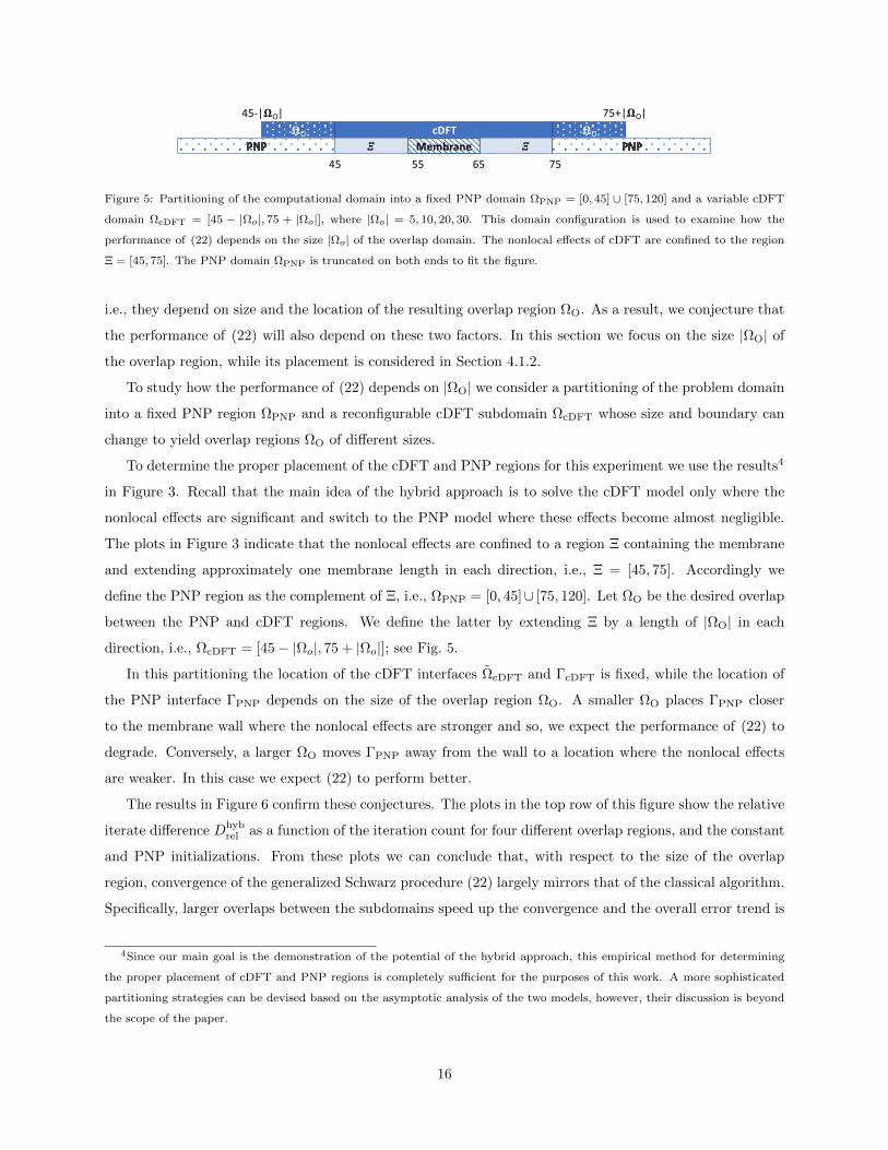
Figure 5: Partitioning of the computational domain into a fixed PNP domain ΩPNP = [0, 45] ∪ [75, 120] and a variable cDFT

domain ΩcDFT = [45 − |Ωo|, 75 + |Ωo|], where |Ωo| = 5, 10, 20, 30. This domain configuration is used to examine how the

performance of (22) depends on the size |Ωo| of the overlap domain. The nonlocal effects of cDFT are confined to the region

Ξ = [45, 75]. The PNP domain ΩPNP is truncated on both ends to fit the figure.

i.e., they depend on size and the location of the resulting overlap region ΩO. As a result, we conjecture that

the performance of (22) will also depend on these two factors. In this section we focus on the size |ΩO| of

the overlap region, while its placement is considered in Section 4.1.2.

To study how the performance of (22) depends on |ΩO| we consider a partitioning of the problem domain

into a fixed PNP region ΩPNP and a reconfigurable cDFT subdomain ΩcDFT whose size and boundary can

change to yield overlap regions ΩO of different sizes.

To determine the proper placement of the cDFT and PNP regions for this experiment we use the results4

in Figure 3. Recall that the main idea of the hybrid approach is to solve the cDFT model only where the

nonlocal effects are significant and switch to the PNP model where these effects become almost negligible.

The plots in Figure 3 indicate that the nonlocal effects are confined to a region Ξ containing the membrane

and extending approximately one membrane length in each direction, i.e., Ξ = [45, 75]. Accordingly we

define the PNP region as the complement of Ξ, i.e., ΩPNP = [0, 45]∪ [75, 120]. Let ΩO be the desired overlap

between the PNP and cDFT regions. We define the latter by extending Ξ by a length of |ΩO| in each

direction, i.e., ΩcDFT = [45− |Ωo|, 75 + |Ωo|]; see Fig. 5.

In this partitioning the location of the cDFT interfaces ΩcDFT and ΓcDFT is fixed, while the location of

the PNP interface ΓPNP depends on the size of the overlap region ΩO. A smaller ΩO places ΓPNP closer

to the membrane wall where the nonlocal effects are stronger and so, we expect the performance of (22) to

degrade. Conversely, a larger ΩO moves ΓPNP away from the wall to a location where the nonlocal effects

are weaker. In this case we expect (22) to perform better.

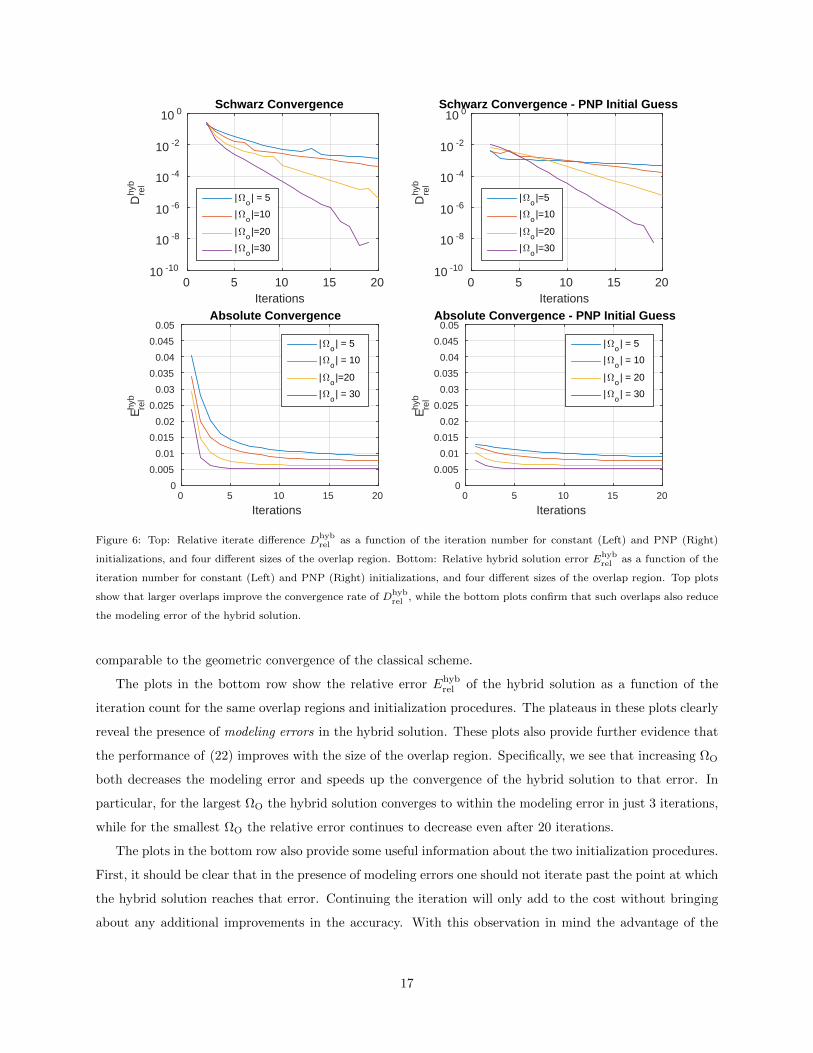
The results in Figure 6 confirm these conjectures. The plots in the top row of this figure show the relative

iterate difference Dhybrel as a function of the iteration count for four different overlap regions, and the constant

and PNP initializations. From these plots we can conclude that, with respect to the size of the overlap

region, convergence of the generalized Schwarz procedure (22) largely mirrors that of the classical algorithm.

Specifically, larger overlaps between the subdomains speed up the convergence and the overall error trend is

4Since our main goal is the demonstration of the potential of the hybrid approach, this empirical method for determining

the proper placement of cDFT and PNP regions is completely sufficient for the purposes of this work. A more sophisticated

partitioning strategies can be devised based on the asymptotic analysis of the two models, however, their discussion is beyond

the scope of the paper.

16

Iterations0 5 10 15 20

Dhy

bre

l

10 -10

10 -8

10 -6

10 -4

10 -2

10 0Schwarz Convergence

|+o| = 5

|+o|=10

|+o|=20

|+o|=30

Iterations0 5 10 15 20

Dhy

bre

l

10 -10

10 -8

10 -6

10 -4

10 -2

10 0Schwarz Convergence - PNP Initial Guess

|+o|=5

|+o|=10

|+o|=20

|+o|=30

Iterations0 5 10 15 20

Ehyb

rel

0

0.005

0.01

0.015

0.02

0.025

0.03

0.035

0.04

0.045

0.05Absolute Convergence

|+o| = 5

|+o| = 10

|+o|=20

|+o| = 30

Iterations0 5 10 15 20

Ehyb

rel

0

0.005

0.01

0.015

0.02

0.025

0.03

0.035

0.04

0.045

0.05Absolute Convergence - PNP Initial Guess

|+o| = 5

|+o| = 10

|+o| = 20

|+o| = 30

Figure 6: Top: Relative iterate difference Dhybrel as a function of the iteration number for constant (Left) and PNP (Right)

initializations, and four different sizes of the overlap region. Bottom: Relative hybrid solution error Ehybrel as a function of the

iteration number for constant (Left) and PNP (Right) initializations, and four different sizes of the overlap region. Top plots

show that larger overlaps improve the convergence rate of Dhybrel , while the bottom plots confirm that such overlaps also reduce

the modeling error of the hybrid solution.

comparable to the geometric convergence of the classical scheme.

The plots in the bottom row show the relative error Ehybrel of the hybrid solution as a function of the

iteration count for the same overlap regions and initialization procedures. The plateaus in these plots clearly

reveal the presence of modeling errors in the hybrid solution. These plots also provide further evidence that

the performance of (22) improves with the size of the overlap region. Specifically, we see that increasing ΩO

both decreases the modeling error and speeds up the convergence of the hybrid solution to that error. In

particular, for the largest ΩO the hybrid solution converges to within the modeling error in just 3 iterations,

while for the smallest ΩO the relative error continues to decrease even after 20 iterations.

The plots in the bottom row also provide some useful information about the two initialization procedures.

First, it should be clear that in the presence of modeling errors one should not iterate past the point at which

the hybrid solution reaches that error. Continuing the iteration will only add to the cost without bringing

about any additional improvements in the accuracy. With this observation in mind the advantage of the

17

x0 20 40 60 80 100 120

-2

0

2

4

6

8

;+ / < ;+ >

;- / < ;- >;0 / < ;0>? / < ?>

(a) Iteration 1

x0 20 40 60 80 100 120

-2

0

2

4

6

8

;+ / < ;+ >

;- / < ;- >;0 / < ;0>? / < ?>

(b) Iteration 2

x0 20 40 60 80 100 120

-2

0

2

4

6

8

;+ / < ;+ >

;- / < ;- >;0 / < ;0>? / < ?>

(c) Iteration 7

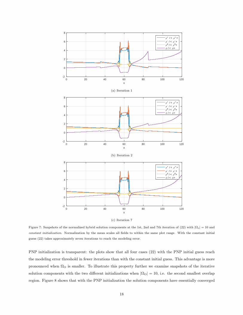
Figure 7: Snapshots of the normalized hybrid solution components at the 1st, 2nd and 7th iteration of (22) with |Ωo| = 10 and

constant initialization. Normalization by the mean scales all fields to within the same plot range. With the constant initial

guess (22) takes approximately seven iterations to reach the modeling error.

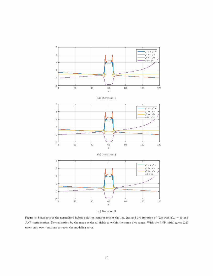
PNP initialization is transparent: the plots show that all four cases (22) with the PNP initial guess reach

the modeling error threshold in fewer iterations than with the constant initial guess. This advantage is more

pronounced when ΩO is smaller. To illustrate this property further we examine snapshots of the iterative

solution components with the two different initializations when |ΩO| = 10, i.e. the second smallest overlap

region. Figure 8 shows that with the PNP initialization the solution components have essentially converged

18

x0 20 40 60 80 100 120

-2

0

2

4

6

8

;+ / < ;+ >

;- / < ;- >;0 / < ;0>? / < ?>

(a) Iteration 1

x0 20 40 60 80 100 120

-2

0

2

4

6

8

;+ / < ;+ >

;- / < ;- >;0 / < ;0>? / < ?>

(b) Iteration 2

x0 20 40 60 80 100 120

-2

0

2

4

6

8

;+ / < ;+ >

;- / < ;- >;0 / < ;0>? / < ?>

(c) Iteration 3

Figure 8: Snapshots of the normalized hybrid solution components at the 1st, 2nd and 3rd iteration of (22) with |Ωo| = 10 and

PNP initialization. Normalization by the mean scales all fields to within the same plot range. With the PNP initial guess (22)

takes only two iterations to reach the modeling error.

19

cDFTMembrane

44 76

54 55 65 66

cDFTMembrane

42 78

52 55 65 68

cDFTMembrane

40 80

50 55 65 70

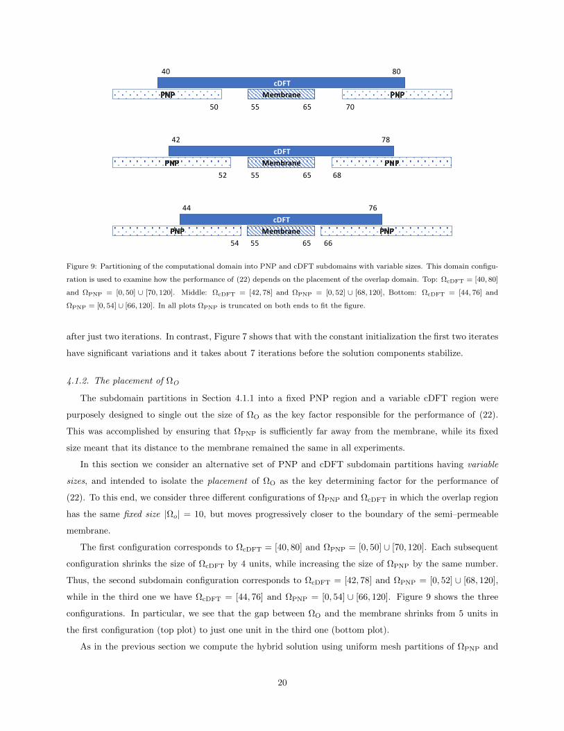
Figure 9: Partitioning of the computational domain into PNP and cDFT subdomains with variable sizes. This domain configu-

ration is used to examine how the performance of (22) depends on the placement of the overlap domain. Top: ΩcDFT = [40, 80]

and ΩPNP = [0, 50] ∪ [70, 120]. Middle: ΩcDFT = [42, 78] and ΩPNP = [0, 52] ∪ [68, 120], Bottom: ΩcDFT = [44, 76] and

ΩPNP = [0, 54] ∪ [66, 120]. In all plots ΩPNP is truncated on both ends to fit the figure.

after just two iterations. In contrast, Figure 7 shows that with the constant initialization the first two iterates

have significant variations and it takes about 7 iterations before the solution components stabilize.

4.1.2. The placement of ΩO

The subdomain partitions in Section 4.1.1 into a fixed PNP region and a variable cDFT region were

purposely designed to single out the size of ΩO as the key factor responsible for the performance of (22).

This was accomplished by ensuring that ΩPNP is sufficiently far away from the membrane, while its fixed

size meant that its distance to the membrane remained the same in all experiments.

In this section we consider an alternative set of PNP and cDFT subdomain partitions having variable

sizes, and intended to isolate the placement of ΩO as the key determining factor for the performance of

(22). To this end, we consider three different configurations of ΩPNP and ΩcDFT in which the overlap region

has the same fixed size |Ωo| = 10, but moves progressively closer to the boundary of the semi–permeable

membrane.

The first configuration corresponds to ΩcDFT = [40, 80] and ΩPNP = [0, 50] ∪ [70, 120]. Each subsequent

configuration shrinks the size of ΩcDFT by 4 units, while increasing the size of ΩPNP by the same number.

Thus, the second subdomain configuration corresponds to ΩcDFT = [42, 78] and ΩPNP = [0, 52] ∪ [68, 120],

while in the third one we have ΩcDFT = [44, 76] and ΩPNP = [0, 54] ∪ [66, 120]. Figure 9 shows the three

configurations. In particular, we see that the gap between ΩO and the membrane shrinks from 5 units in

the first configuration (top plot) to just one unit in the third one (bottom plot).

As in the previous section we compute the hybrid solution using uniform mesh partitions of ΩPNP and

20

x0 20 40 60 80 100 120

-2

0

2

4

6

8

x0 20 40 60 80 100 120

-2

0

2

4

6

8

x0 20 40 60 80 100 120

-2

0

2

4

6

8

10

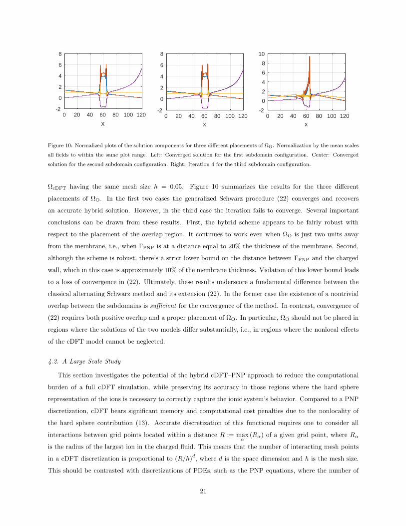
Figure 10: Normalized plots of the solution components for three different placements of ΩO. Normalization by the mean scales

all fields to within the same plot range. Left: Converged solution for the first subdomain configuration. Center: Converged

solution for the second subdomain configuration. Right: Iteration 4 for the third subdomain configuration.

ΩcDFT having the same mesh size h = 0.05. Figure 10 summarizes the results for the three different

placements of ΩO. In the first two cases the generalized Schwarz procedure (22) converges and recovers

an accurate hybrid solution. However, in the third case the iteration fails to converge. Several important

conclusions can be drawn from these results. First, the hybrid scheme appears to be fairly robust with

respect to the placement of the overlap region. It continues to work even when ΩO is just two units away

from the membrane, i.e., when ΓPNP is at a distance equal to 20% the thickness of the membrane. Second,

although the scheme is robust, there’s a strict lower bound on the distance between ΓPNP and the charged

wall, which in this case is approximately 10% of the membrane thickness. Violation of this lower bound leads

to a loss of convergence in (22). Ultimately, these results underscore a fundamental difference between the

classical alternating Schwarz method and its extension (22). In the former case the existence of a nontrivial

overlap between the subdomains is sufficient for the convergence of the method. In contrast, convergence of

(22) requires both positive overlap and a proper placement of ΩO. In particular, ΩO should not be placed in

regions where the solutions of the two models differ substantially, i.e., in regions where the nonlocal effects

of the cDFT model cannot be neglected.

4.2. A Large Scale Study

This section investigates the potential of the hybrid cDFT–PNP approach to reduce the computational

burden of a full cDFT simulation, while preserving its accuracy in those regions where the hard sphere

representation of the ions is necessary to correctly capture the ionic system’s behavior. Compared to a PNP

discretization, cDFT bears significant memory and computational cost penalties due to the nonlocality of

the hard sphere contribution (13). Accurate discretization of this functional requires one to consider all

interactions between grid points located within a distance R := maxα

(Rα) of a given grid point, where Rα

is the radius of the largest ion in the charged fluid. This means that the number of interacting mesh points

in a cDFT discretization is proportional to (R/h)d, where d is the space dimension and h is the mesh size.

This should be contrasted with discretizations of PDEs, such as the PNP equations, where the number of

21

interacting mesh points remains constant5 under uniform mesh refinement because it depends on the mesh

topology and the order of the method but not on the mesh size h.

These differences have a significant impact on the sparsity structure of the corresponding Jacobians,

which are required for the numerical solution of the nonlinear systems of algebraic equations resulting from

the discretization of the cDFT and PNP equations. In both cases the number of rows in each Jacobian equals

the number of degrees of freedom n in the mesh, which is proportional to (1/h)d. Let K > 0 be an upper

bound on the number of interacting mesh points in the PNP discretization. Then, the number of nonzero

elements in the PNP Jacobian is proportional to(1

h

)dK = nK,

that is, it depends linearly on the number of degrees of freedom. In contrast, the number of nonzero elements

in the cDFT Jacobian is proportional to(1

h

)d(R

h

)d=

(1

hd

)2

Rd = n2Rd, (25)

that is, this number grows as the square of the number of degrees of freedom. As a result, both the memory

requirements and the computational costs of a full cDFT simulation can quickly become prohibitive when

solving large 2D or 3D problems6.

To provide a more realistic assessment of the cost and memory savings of the hybrid approach we use

the two-dimensional setting of Example 2, i.e., the potential–driven channel flow problem shown in Figure 2.

We recall that in this example one makes the assumption that flow is symmetric along the channel’s axis,

which allows us to simulate only one half of the channel.

The dimensions of the domain are Ω = [0, 1600] × [0, 204]. The surface charge of the left half of the

channel is set to −0.3, and the surface charge of the right half of the channel is set to zero. We consider

a three-component ionic system comprising positive, negative and neutral species. The cation and neutral

ion diameters are chosen to be 1 and the anion diameter is chosen to be 1.5. To complete the problem

specification we set the bulk density for all charged species to 0.0016 on both sides of the channel. For the

neutral species the bulk density is also the same on both sides but is set to 0.7. We refer to Figure 2 for an

illustration of the problem configuration.

In our study we compare large scale simulations of this problem using a full cDFT, a full PNP and a

hybrid discretization of the governing equations. For the full cDFT and PNP simulations we use a sequence

5For more general refinement policies one can show that the number of interacting mesh points is bounded from above

independently of the mesh size if the refinement is constrained to produce only shape-regular grids.6There have been some recent efforts [44] to reduce the memory requirements and the computational costs of non-local

methods for fractional order PDEs by using Hierarchic matrices (H-matrices). However, the application of these ideas to cDFT

requires a rigorous mathematical basis, which to the best of our knowledge has not been yet developed. As a result, none of

the available cDFT codes use these techniques.

22

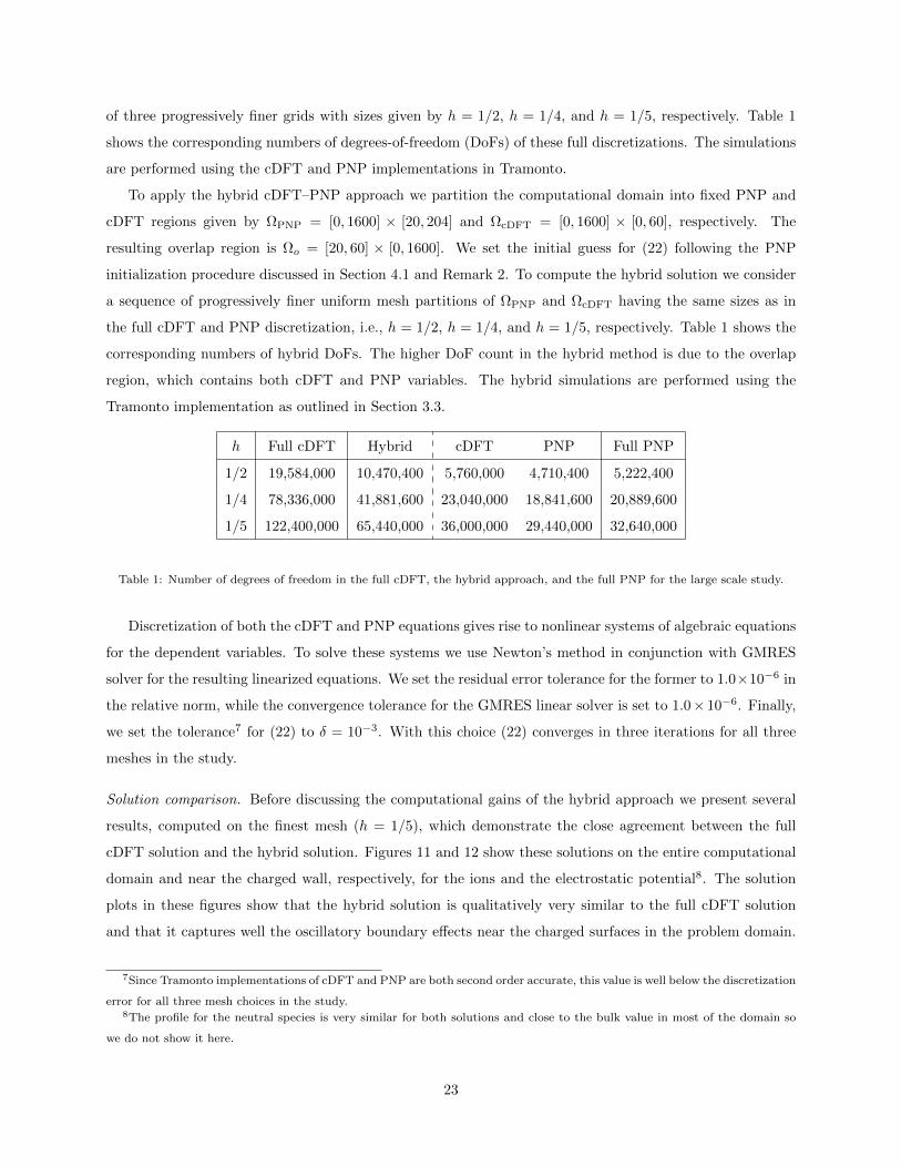
of three progressively finer grids with sizes given by h = 1/2, h = 1/4, and h = 1/5, respectively. Table 1

shows the corresponding numbers of degrees-of-freedom (DoFs) of these full discretizations. The simulations

are performed using the cDFT and PNP implementations in Tramonto.

To apply the hybrid cDFT–PNP approach we partition the computational domain into fixed PNP and

cDFT regions given by ΩPNP = [0, 1600] × [20, 204] and ΩcDFT = [0, 1600] × [0, 60], respectively. The

resulting overlap region is Ωo = [20, 60] × [0, 1600]. We set the initial guess for (22) following the PNP

initialization procedure discussed in Section 4.1 and Remark 2. To compute the hybrid solution we consider

a sequence of progressively finer uniform mesh partitions of ΩPNP and ΩcDFT having the same sizes as in

the full cDFT and PNP discretization, i.e., h = 1/2, h = 1/4, and h = 1/5, respectively. Table 1 shows the

corresponding numbers of hybrid DoFs. The higher DoF count in the hybrid method is due to the overlap

region, which contains both cDFT and PNP variables. The hybrid simulations are performed using the

Tramonto implementation as outlined in Section 3.3.

h Full cDFT Hybrid cDFT PNP Full PNP

1/2 19,584,000 10,470,400 5,760,000 4,710,400 5,222,400

1/4 78,336,000 41,881,600 23,040,000 18,841,600 20,889,600

1/5 122,400,000 65,440,000 36,000,000 29,440,000 32,640,000

Table 1: Number of degrees of freedom in the full cDFT, the hybrid approach, and the full PNP for the large scale study.

Discretization of both the cDFT and PNP equations gives rise to nonlinear systems of algebraic equations

for the dependent variables. To solve these systems we use Newton’s method in conjunction with GMRES

solver for the resulting linearized equations. We set the residual error tolerance for the former to 1.0×10−6 in

the relative norm, while the convergence tolerance for the GMRES linear solver is set to 1.0× 10−6. Finally,

we set the tolerance7 for (22) to δ = 10−3. With this choice (22) converges in three iterations for all three

meshes in the study.

Solution comparison. Before discussing the computational gains of the hybrid approach we present several

results, computed on the finest mesh (h = 1/5), which demonstrate the close agreement between the full

cDFT solution and the hybrid solution. Figures 11 and 12 show these solutions on the entire computational

domain and near the charged wall, respectively, for the ions and the electrostatic potential8. The solution

plots in these figures show that the hybrid solution is qualitatively very similar to the full cDFT solution

and that it captures well the oscillatory boundary effects near the charged surfaces in the problem domain.

7Since Tramonto implementations of cDFT and PNP are both second order accurate, this value is well below the discretization

error for all three mesh choices in the study.8The profile for the neutral species is very similar for both solutions and close to the bulk value in most of the domain so

we do not show it here.

23

In contrast, Figure 13 reveals that the full PNP solution on the same mesh completely misses these effects.

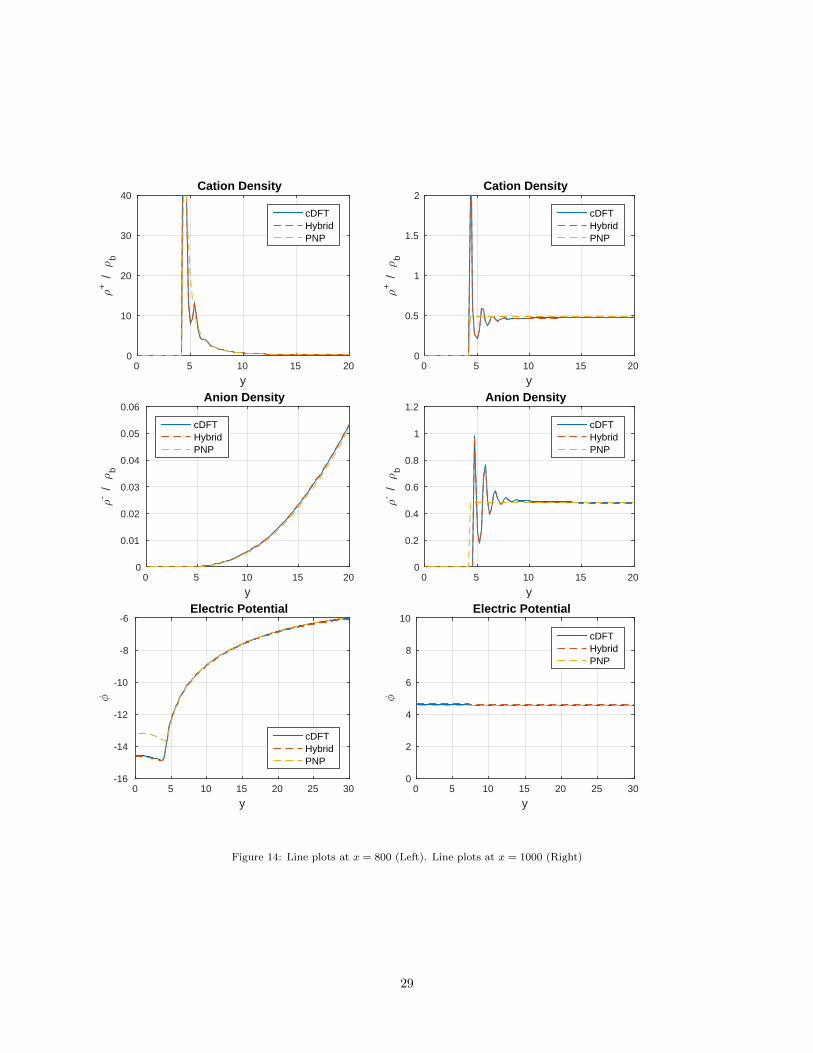
For a more quantitative assessment of the full cDFT, hybrid and full PNP solutions, Figure 14 compares

their cross-sections at two different locations along the channel, given by x = 800 and x = 1000, respectively.

The first location, x = 800, corresponds to the edge of the negatively charged surface. There, the cations are

strongly absorbed to the surface and develop a characteristic double layer profile. Both the full cDFT and

the hybrid solution correctly represent this double layer and also capture some smaller oscillations9 in the

cation density profile. We also note that both the cDFT and the hybrid solutions have considerably higher

contact densities than the full PNP solutions. As a result, in the density profile, the former develop a more

narrow peak near the wall than the latter. We also see that the electrostatic potential near the surface is

different in the PNP solution than in the cDFT and hybrid solutions, so the zeta potential (potential at the

surface) is different, in this case by 1.4 kT/e = 36 mV. We’ll say more about this shortly.

At the second location, i.e., x = 1000, the surface is neutral and there is no double layer. However the

hard sphere contribution (13) in the cDFT model supports packing effects, which prompt oscillatory density

profiles in the full cDFT solution. In particular, due to their larger size the anions in this solution are located

further from the surface. Figure 14 shows that the hybrid solution captures accurately these effects and is

in excellent agreement with the full cDFT solution. In contrast, the idealization of the ions as point charges

in the PNP model completely misses the packing effects and leads to uniform density profiles.

It is worth pointing out that near the neutral surface the electrostatic potentials are nearly identical for all

three solutions. This behavior is likely due to the following two factors. First, both the PNP and the cDFT

models share the same Poisson equation (1) for the electrostatic potential. Second, near the neutral surface

the cDFT densities oscillate symmetrically around the constant PNP densities, i.e., their mean values are

very close. As a result, although oscillatory, the cDFT densities should give roughly the same total charge

density values as the PNP densities, because (3) computes a weighted average of these quantities. In contrast,

near the charged wall the cDFT densities are not symmetric relative to the PNP densities and so, they will

have different mean values. As a result, the total charge density will differ for the two models, which explains

the different potentials. Note that this difference is confined to a region that correlates exactly with the

extent of the oscillatory behavior in the cation density profile.

Computational performance. We now examine the computational performance of the hybrid approach vs.

the full cDFT and full PNP simulations. Table 2 shows the wall clock times for each simulation, normalized

by the time of the full cDFT simulation on the coarsest mesh, i.e., h = 1/2, while Table 3 provides information

about the dimensions of the Krylov subspaces Kr in the GMRES solver required for the different methods.

The last two columns in Table 2 reveal two interesting trends10. First, with respect to the full cDFT

9These oscillations are a smaller effect than the large adsorption due to electrostatics.10Although the study is limited to three different mesh sizes, the large dimensions of the resulting discrete problems give us

some confidence that the observed behavior of the methods is in their respective asymptotic regimes.

24

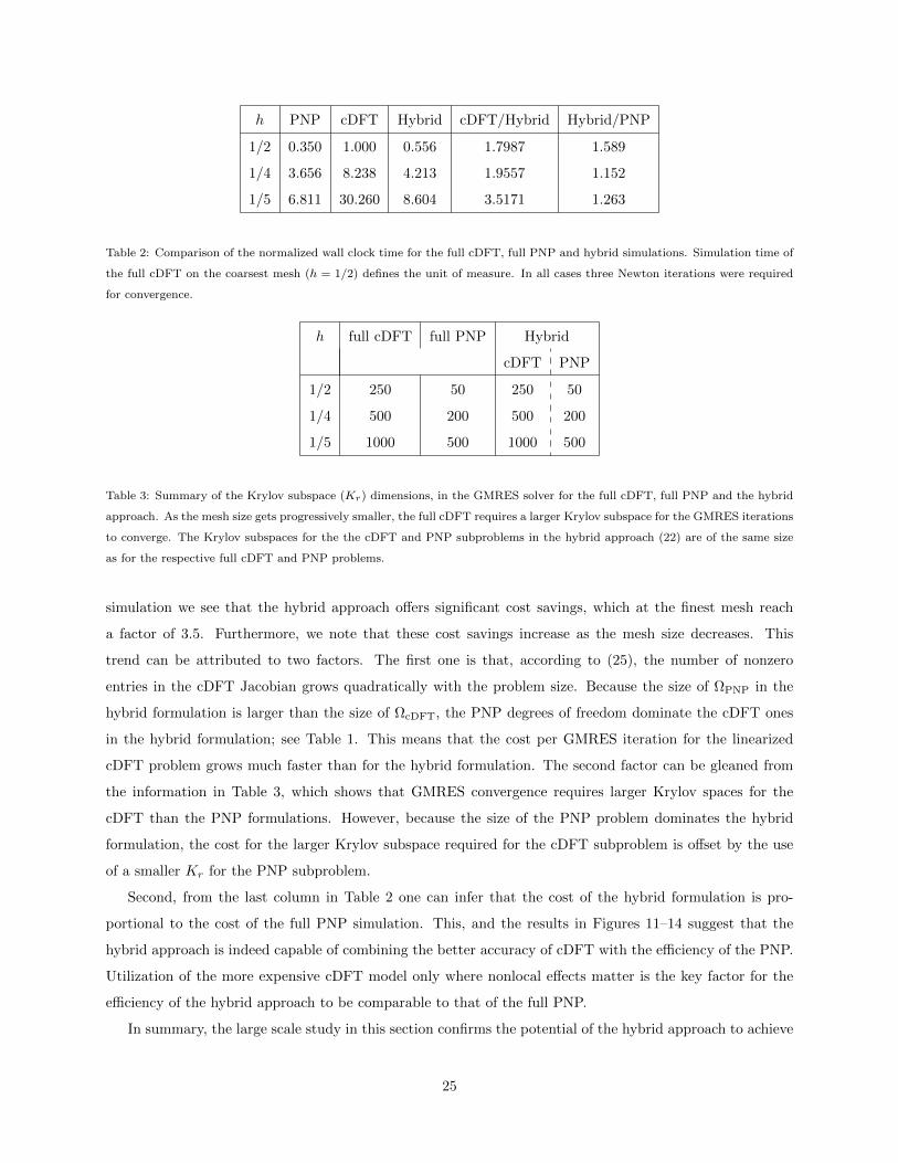
h PNP cDFT Hybrid cDFT/Hybrid Hybrid/PNP

1/2 0.350 1.000 0.556 1.7987 1.589

1/4 3.656 8.238 4.213 1.9557 1.152

1/5 6.811 30.260 8.604 3.5171 1.263

Table 2: Comparison of the normalized wall clock time for the full cDFT, full PNP and hybrid simulations. Simulation time of

the full cDFT on the coarsest mesh (h = 1/2) defines the unit of measure. In all cases three Newton iterations were required

for convergence.

h full cDFT full PNP Hybrid

cDFT PNP

1/2 250 50 250 50

1/4 500 200 500 200

1/5 1000 500 1000 500

Table 3: Summary of the Krylov subspace (Kr) dimensions, in the GMRES solver for the full cDFT, full PNP and the hybrid

approach. As the mesh size gets progressively smaller, the full cDFT requires a larger Krylov subspace for the GMRES iterations

to converge. The Krylov subspaces for the the cDFT and PNP subproblems in the hybrid approach (22) are of the same size

as for the respective full cDFT and PNP problems.

simulation we see that the hybrid approach offers significant cost savings, which at the finest mesh reach

a factor of 3.5. Furthermore, we note that these cost savings increase as the mesh size decreases. This

trend can be attributed to two factors. The first one is that, according to (25), the number of nonzero

entries in the cDFT Jacobian grows quadratically with the problem size. Because the size of ΩPNP in the

hybrid formulation is larger than the size of ΩcDFT, the PNP degrees of freedom dominate the cDFT ones

in the hybrid formulation; see Table 1. This means that the cost per GMRES iteration for the linearized

cDFT problem grows much faster than for the hybrid formulation. The second factor can be gleaned from

the information in Table 3, which shows that GMRES convergence requires larger Krylov spaces for the

cDFT than the PNP formulations. However, because the size of the PNP problem dominates the hybrid

formulation, the cost for the larger Krylov subspace required for the cDFT subproblem is offset by the use

of a smaller Kr for the PNP subproblem.

Second, from the last column in Table 2 one can infer that the cost of the hybrid formulation is pro-

portional to the cost of the full PNP simulation. This, and the results in Figures 11–14 suggest that the

hybrid approach is indeed capable of combining the better accuracy of cDFT with the efficiency of the PNP.

Utilization of the more expensive cDFT model only where nonlocal effects matter is the key factor for the

efficiency of the hybrid approach to be comparable to that of the full PNP.

In summary, the large scale study in this section confirms the potential of the hybrid approach to achieve

25

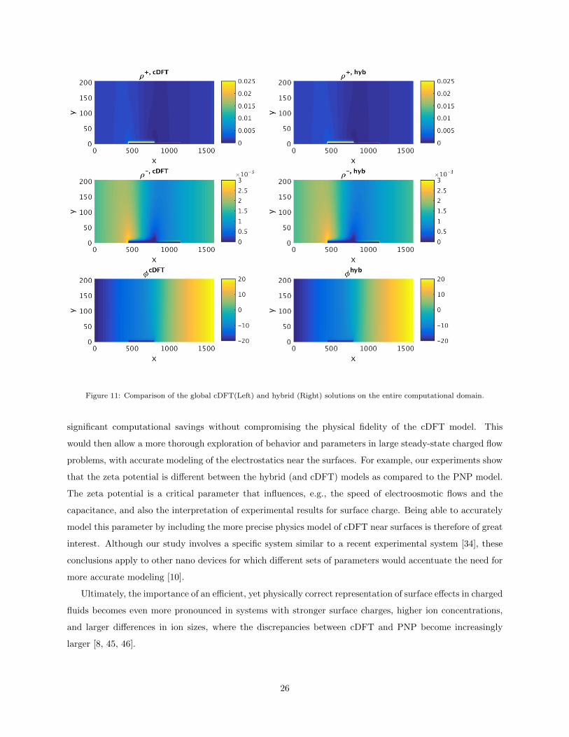
Figure 11: Comparison of the global cDFT(Left) and hybrid (Right) solutions on the entire computational domain.

significant computational savings without compromising the physical fidelity of the cDFT model. This

would then allow a more thorough exploration of behavior and parameters in large steady-state charged flow

problems, with accurate modeling of the electrostatics near the surfaces. For example, our experiments show

that the zeta potential is different between the hybrid (and cDFT) models as compared to the PNP model.

The zeta potential is a critical parameter that influences, e.g., the speed of electroosmotic flows and the

capacitance, and also the interpretation of experimental results for surface charge. Being able to accurately

model this parameter by including the more precise physics model of cDFT near surfaces is therefore of great

interest. Although our study involves a specific system similar to a recent experimental system [34], these

conclusions apply to other nano devices for which different sets of parameters would accentuate the need for

more accurate modeling [10].

Ultimately, the importance of an efficient, yet physically correct representation of surface effects in charged

fluids becomes even more pronounced in systems with stronger surface charges, higher ion concentrations,

and larger differences in ion sizes, where the discrepancies between cDFT and PNP become increasingly

larger [8, 45, 46].

26

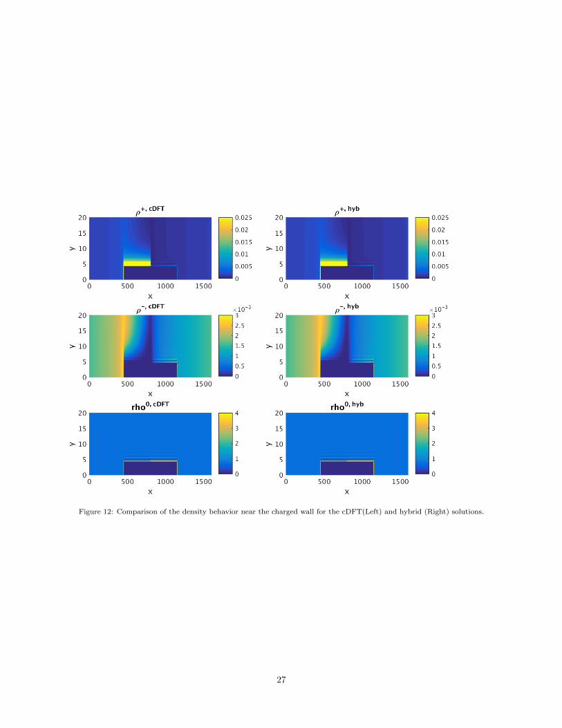
Figure 12: Comparison of the density behavior near the charged wall for the cDFT(Left) and hybrid (Right) solutions.

27

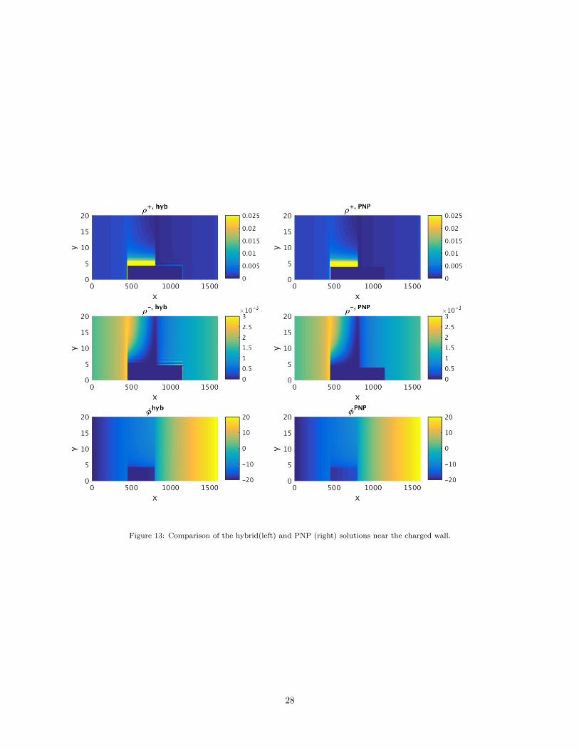
Figure 13: Comparison of the hybrid(left) and PNP (right) solutions near the charged wall.

28

y0 5 10 15 20

;+

/ ;

b

0

10

20

30

40Cation Density

cDFTHybridPNP

y0 5 10 15 20

;+

/ ;

b

0

0.5

1

1.5

2Cation Density

cDFTHybridPNP

y0 5 10 15 20

;- / ;

b

0

0.01

0.02

0.03

0.04

0.05

0.06Anion Density

cDFTHybridPNP

y0 5 10 15 20

;- / ;

b

0

0.2

0.4

0.6

0.8

1

1.2Anion Density

cDFTHybridPNP

y0 5 10 15 20 25 30

?

-16

-14

-12

-10

-8

-6Electric Potential

cDFTHybridPNP

y0 5 10 15 20 25 30

?

0

2

4

6

8

10Electric Potential

cDFTHybridPNP

Figure 14: Line plots at x = 800 (Left). Line plots at x = 1000 (Right)

29

5. Conclusion

In this work we have developed a hybrid simulation approach for ionic systems, which allows us to

combine the accuracy of the nonlocal cDFT model with the efficiency of the PNP equations. The motivation

for this approach stems from the fact that in many modeling and simulation scenarios the higher fidelity of

the cDFT model is required only near surfaces in the problem domain, while the PNP equations provide an

adequate representation of the physics in the rest of the domain.

To develop the approach we formulate a coupled hybrid cDFT–PNP model in which the cDFT and PNP

equations operate independently on two overlapping domains, subject to suitable coupling conditions. We

then solve this coupled problem iteratively by applying the principles of the classical alternating Schwarz

method to the hybrid system. In particular, the coupling conditions serve to define the boundary conditions

and volume constraints exchanged between the two models.

Numerical examples show that in many ways the new hybrid approach behaves much like the classical

Schwarz method, for instance, its convergence depends on the overlap between the two subdomains. However,

unlike the classical scheme, where the size of the overlap is the only convergence factor, performance of the

hybrid approach also depends on the proper placement of the overlap region. Our experiments show that

this region must be located sufficiently far away from the surfaces where the nonlocal effects of cDFT become

almost negligible.

Finally, the large scale study of a nano device in two dimensions confirmed the potential of the hybrid

approach to significantly reduce the computational cost, while retaining the accuracy of cDFT near the

surfaces. We anticipate that even more significant savings can be realized by using the hybrid approach for

three-dimensional simulations. Its extension to this setting is straightforward.

6. Acknowledgments

This work was supported by the U.S. Department of Energy Office of Science, Office of Advanced Scien-

tific Computing Research, Applied Mathematics program as part of the Collaboratory on Mathematics for

Mesoscopic Modeling of Materials (CM4), under Award Number DE-SC0009247. Sandia National Laborato-

ries is a multi-mission laboratory managed and operated by Sandia Corporation, a wholly owned subsidiary

of Lockheed Martin Corporation, for the U.S. Department of Energy’s National Nuclear Security Adminis-

tration under contract DE-AC04-94AL85000.

References

[1] Z. Yuan, A. L. Garcia, G. P. Lopez, D. N. Petsev, Electrokinetic transport and separations in fluidic

nanochannels, ELECTROPHORESIS 28 (4) (2007) 595–610.

[2] M. Napoli, J. C. T. Eijkel, S. Pennathur, Nanofluidic technology for biomolecule applications: a critical

review, Lab Chip 10 (8) (2010) 957.

30

[3] P. Magnico, Influence of the ion–solvent interactions on ionic transport through ion-exchange-

membranes, J Membrane Sci 442 (2013) 272–285.

[4] R. S. Eisenberg, Computing the field in proteins and channels, Journal of Membrane Biology 150 (1)

(1996) 1–25.

[5] R. Evans, The nature of the liquid-vapour interface and other topics in the statistical mechanics of non-

uniform, classical fluids, Advances in Physics 28 (2) (1979) 143–200. doi:10.1080/00018737900101365.

[6] D. Henderson, S. Lamperski, Z. Jin, J. Wu, Density Functional Study of the Electric Double Layer

Formed by a High Density Electrolyte, J Phys Chem B 115 (44) (2011) 12911–12914.

[7] L. B. Bhuiyan, S. Lamperski, J. Wu, D. Henderson, Monte Carlo Simulation for the Double Layer

Structure of an Ionic Liquid Using a Dimer Model: A Comparison with the Density Functional Theory,

J Phys Chem B 116 (34) (2012) 10364–10370.

[8] D. Gillespie, A. S. Khair, J. P. Bardhan, S. Pennathur, Efficiently accounting for ion correlations in

electrokinetic nanofluidic devices using density functional theory, J Colloid Interf Sci 359 (2) (2011)

520–529.

[9] J. Hoffmann, D. Gillespie, Ion Correlations in Nanofluidic Channels: Effects of Ion Size, Valence, and

Concentration on Voltage- and Pressure-Driven Currents, Langmuir 29 (4) (2013) 1303–1317.

[10] F. H. J. van der Heyden, D. Stein, K. Besteman, S. G. Lemay, C. Dekker, Charge Inversion at High

Ionic Strength Studied by Streaming Currents, Phys Rev Lett 96 (22) (2006) 224502.

[11] S. Badia, P. Bochev, M. Gunzburger, R. Lehoucq, M. Parks, Blending methods for coupling atom-

istic and continuum models, in: J. Fish (Ed.), Bridging the scales in science and engineering, Oxford

University Press, 2009, pp. 165–186. doi:doi:10.1093/acprof:oso/9780199233854.001.0001.

[12] H. B. Dhia, G. Rateau, The Arlequin method as a flexible engineering design tool, International Journal

for Numerical Methods in Engineering 62 (11) (2005) 1442–1462. doi:10.1002/nme.1229.

URL http://dx.doi.org/10.1002/nme.1229

[13] M. Luskin, C. Ortner, B. V. Koten, Formulation and optimization of the energy-based blended qua-

sicontinuum method, Computer Methods in Applied Mechanics and Engineering 253 (0) (2013) 160 –

168. doi:10.1016/j.cma.2012.09.007.

URL http://www.sciencedirect.com/science/article/pii/S0045782512002824

[14] P. Seleson, S. Beneddine, S. Prudhomme, A force-based coupling scheme for peri-

dynamics and classical elasticity, Computational Materials Science 66 (2013) 34–49.

doi:http://dx.doi.org/10.1016/j.commatsci.2012.05.016.

URL http://www.sciencedirect.com/science/article/pii/S092702561200287X

31

[15] Y. Azdoud, F. Han, G. Lubineau, A morphing framework to couple non-local and local

anisotropic continua, International Journal of Solids and Structures 50 (9) (2013) 1332 – 1341.

doi:http://dx.doi.org/10.1016/j.ijsolstr.2013.01.016.

URL http://www.sciencedirect.com/science/article/pii/S0020768313000310

[16] G. Lubineau, Y. Azdoud, F. Han, C. Rey, A. Askari, A morphing strategy to couple non-local to

local continuum mechanics, Journal of the Mechanics and Physics of Solids 60 (6) (2012) 1088 – 1102.

doi:http://dx.doi.org/10.1016/j.jmps.2012.02.009.

[17] M. D’Elia, P. B. Bochev, Optimization-based coupling of nonlocal and local diffusion models, in: Sympo-

sium NN, Mathematical and Computational Aspects of Materials Science, Vol. 1753 of MRS Proceedings,

2015.

[18] M. D’Elia, M. Perego, P. B. Bochev, D. Littlewood, A coupling strategy for nonlocal and local diffu-

sion models with mixed volume constraints and boundary conditions, Computers & Mathematics with

Applicationsdoi:http://dx.doi.org/10.1016/j.camwa.2015.12.006.

[19] D. Olson, P. Bochev, M. Luskin, A. Shapeev, An optimization-based atomistic-to-

continuum coupling method, SIAM Journal on Numerical Analysis 52 (4) (2014) 2183–2204.

arXiv:http://dx.doi.org/10.1137/13091734X, doi:10.1137/13091734X.

URL http://dx.doi.org/10.1137/13091734X

[20] Olson, Derek, Shapeev, Alexander V., Bochev, Pavel B., Luskin, Mitchell, Analysis of an optimization-

based atomistic-to-continuum coupling method for point defects, ESAIM: M2AN 50 (1) (2016) 1–41.

doi:10.1051/m2an/2015023.

URL http://dx.doi.org/10.1051/m2an/2015023

[21] A. Abdulle, O. Jecker, A. Shapeev, An optimization based coupling method for multiscale problems,

MATHICSE 26.2015, EPFL, Lausanne, Switzerland, Switzerland (December 2015).

[22] B. Smith, P. Bjorstad, W. Gropp, Domain Decomposition: Parallel Multilevel Methods for Elliptic

Partial Differential Equations, Cambridge University Press, 1996.

[23] M. Parks, P. Bochev, R. Lehoucq, Connecting atomistic-to-continuum coupling and domain decompo-

sition, Multiscale Modeling & Simulation 7 (1) (2008) 362–380. doi:10.1137/070682848.

URL http://link.aip.org/link/?MMS/7/362/1

[24] X. Bian, Z. Li, M. Deng, G. E. Karniadakis, Fluctuating hydrodynamics in periodic domains

and heterogeneous adjacent multidomains: Thermal equilibrium, Phys. Rev. E 92 (2015) 053302.

doi:10.1103/PhysRevE.92.053302.

URL http://link.aps.org/doi/10.1103/PhysRevE.92.053302

32

[25] X. Bian, M. Deng, Y.-H. Tang, G. E. Karniadakis, Analysis of hydrodynamic fluctua-

tions in heterogeneous adjacent multidomains in shear flow, Phys. Rev. E 93 (2016) 033312.

doi:10.1103/PhysRevE.93.033312.

URL http://link.aps.org/doi/10.1103/PhysRevE.93.033312

[26] R. Roth, R. Evans, A. Lang, G. Kahl, Fundamental measure theory for hard-sphere mixtures revisited:

the White Bear version, J Phys-Condens Mat 14 (46) (2002) 12063–12078.

[27] Y.-X. Yu, J. Z. Wu, Structures of hard-sphere fluids from a modified fundamental-measure theory, J

Chem Phys 117 (22) (2002) 10156–10164.

[28] A. Oleksy, J.-P. Hansen, Towards a microscopic theory of wetting by ionic solutions. I. Surface properties

of the semi-primitive model, Mol Phys 104 (18) (2006) 2871–2883.

[29] G. Mansoori, N. Carnahan, K. Starling, T. Leland, Equilibrium thermodynamic properties of misture

of hard spheres, J Chem Phys 54 (4) (1971) 1523–&.

[30] L. J. D. Frink, A. Thompson, A. G. Salinger, Applying molecular theory to steady-state diffusing

systems, J Chem Phys 112 (17) (2000) 7564.

[31] Q. DU, M. GUNZBURGER, R. B. LEHOUCQ, K. ZHOU, A nonlocal vec-

tor calculus, nonlocal volume-constrained problems, and nonlocal balance laws,

Mathematical Models and Methods in Applied Sciences 23 (03) (2013) 493–

540. arXiv:http://www.worldscientific.com/doi/pdf/10.1142/S0218202512500546,

doi:10.1142/S0218202512500546.

URL http://www.worldscientific.com/doi/abs/10.1142/S0218202512500546

[32] P. Magnico, Journal of Membrane Science, J Membrane Sci 415-416 (C) (2012) 412–423.

[33] J. Cervera, B. Schiedt, R. Neumann, S. Mafe, P. Ramirez, Ionic conduction, rectification, and selectivity

in single conical nanopores, J Chem Phys 124 (10) (2006) 104706.

[34] R. Karnik, C. Duan, K. Castelino, H. Daiguji, A. Majumdar, Rectification of ionic current in a nanoflu-

idic diode, Nano Lett 7 (3) (2007) 547–551.

[35] H. Daiguji, Y. Oka, K. Shirono, Nanofluidic diode and bipolar transistor, Nano Lett 5 (11) (2005)

2274–2280.

[36] S. Nasir, M. Ali, P. Ramirez, V. Gomez, B. Oschmann, F. Muench, M. Nawaz Tahir, R. Zentel, S. Mafe,

W. Ensinger, Fabrication of Single Cylindrical Au-Coated Nanopores with Non-Homogeneous Fixed

Charge Distribution Exhibiting High Current Rectifications, ACS Appl. Mater. Interfaces 6 (15) (2014)

12486–12494.

33

[37] S. Wu, F. Wildhaber, A. Bertsch, J. Brugger, P. Renaud, Field effect modulated nanofluidic diode

membrane based on Al2O3/W heterogeneous nanopore arrays, Appl. Phys. Lett. 102 (21) (2013) 213108.

[38] P. L. Lions, On the Schwarz alternating method I, in: R. Glowinski, G. Golub, G. Meurant, J. Periaux

(Eds.), Domain Decomposition Methods for Partial Differential Equations, Proceedings of the 1st In-

ternational Conference on Domain Decomposition Methods in Paris, France (January 7-9 1987), SIAM,

SIAM, Philadelphia, 1988.

[39] M. Gee, C. Siefert, J. Hu, R. Tuminaro, M. Sala, ML 5.0 smoothed aggregation user’s guide, Tech. Rep.

SAND2006-2649 (2006).

[40] M. Heroux, R. Bartlett, e. a. V. Howle, An overview of Trilinos, Tech. Rep. SAND2003-2927 (2003).

[41] L. J. D. Frink, A. G. Salinger, M. P. Sears, J. Weinhold, A. L. Frischknecht, Numerical challenges in the

application of density functional theory to biology and nanotechnology, J Phys-Condens Mat 14 (2002)

12167–12187.

[42] M. A. Heroux, A. G. Salinger, L. J. D. Frink, Parallel segregated Schur complement methods for fluid

density functional theories, SIAM J Sci Comput 29 (5) (2007) 2059–2077.

[43] A. L. Frischknecht, D. O. Halligan, M. L. Parks, Electrical double layers and differential capacitance in

molten salts from density functional theory, J Chem Phys 141 (5) (2014) 054708.

[44] X. Zhao, X. Hu, W. Cai, G. E. Karniadakis, Adaptive finite element method for fractional differential

equations using hierarchical matrices (2016). arXiv:1603.01358.

[45] R. H. Nilson, S. K. Griffiths, Influence of atomistic physics on electro-osmotic flow: An analysis based

on density functional theory, J Chem Phys 125 (16) (2006) 164510.

[46] J. W. Lee, R. H. Nilson, J. A. Templeton, S. K. Griffiths, A. Kung, B. M. Wong, Comparison of

Molecular Dynamics with Classical Density Functional and Poisson–Boltzmann Theories of the Electric

Double Layer in Nanochannels, J Chem Theory Comput 8 (6) (2012) 2012–2022.

34