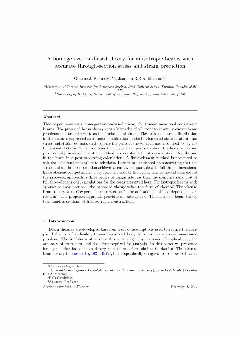
A homogenization-based theory for anisotropic beams withaccurate through-section stress and strain prediction

Graeme J. Kennedya,1,∗, Joaquim R.R.A. Martinsb,2

aUniversity of Toronto Institute for Aerospace Studies, 4925 Dufferin Street, Toronto, Canada, M3H5T6

bUniversity of Michigan, Department of Aerospace Engineering, Ann Arbor, MI 48109

Abstract

This paper presents a homogenization-based theory for three-dimensional anisotropicbeams. The proposed beam theory uses a hierarchy of solutions to carefully-chosen beamproblems that are referred to as the fundamental states. The stress and strain distributionin the beam is expressed as a linear combination of the fundamental state solutions andstress and strain residuals that capture the parts of the solution not accounted for by thefundamental states. This decomposition plays an important role in the homogenizationprocess and provides a consistent method to reconstruct the stress and strain distributionin the beam in a post-processing calculation. A finite-element method is presented tocalculate the fundamental state solutions. Results are presented demonstrating that thestress and strain reconstruction achieves accuracy comparable with full three-dimensionalfinite element computations, away from the ends of the beam. The computational cost ofthe proposed approach is three orders of magnitude less than the computational cost offull three-dimensional calculations for the cases presented here. For isotropic beams withsymmetric cross-sections, the proposed theory takes the form of classical Timoshenkobeam theory with Cowper’s shear correction factor and additional load-dependent cor-rections. The proposed approach provides an extension of Timoshenko’s beam theorythat handles sections with anisotropic construction.

1. Introduction

Beam theories are developed based on a set of assumptions used to reduce the com-plex behavior of a slender, three-dimensional body to an equivalent one-dimensionalproblem. The usefulness of a beam theory is judged by its range of applicability, theaccuracy of its results, and the effort required for analysis. In this paper we present ahomogenization-based beam theory that takes a form similar to classical Timoshenkobeam theory (Timoshenko, 1921, 1922), but is specifically designed for composite beams.

∗Corresponding authorEmail addresses: graeme.kennedy@utoronto.ca (Graeme J. Kennedy), jrram@umich.edu (Joaquim

R.R.A. Martins)1PhD Candidate2Associate Professor

Preprint submitted to Elsevier December 8, 2011

In our approach, we calibrate the stiffness properties, shear strain correction matrix, andload-dependent corrections within the theory based on a hierarchy of solutions that wecall the fundamental states. The fundamental states are accurate sectional stress andstrain solutions to a series of carefully-chosen, statically determinate beam problems.Since it is difficult to obtain exact solutions for the fundamental states for an arbitrarysection, we formulate a finite-element solution technique to obtain approximate solutions.

This paper is structured as follows: In Section 2 we review some important contribu-tions from the relevant literature. In Section 3 we outline the present theory. In Section 4we present the finite-element based technique for the determination of the fundamentalstates. Finally, in Section 5 we present some results from the theory and present compar-isons with full three-dimensional approximate solutions obtained using the finite-elementmethod.

2. Review of relevant contributions

In this section we present a review of various contributions that are most relevant toour proposed beam theory. A comprehensive review of all beam theories is not practicalhere due to the volume of literature that has been produced on the subject over severaldecades.

In two influential papers, Timoshenko (1921, 1922) developed a beam theory forisotropic beams based on a plane stress assumption. Timoshenko’s theory takes intoaccount shear deformation and includes both displacement and rotation variables. Inaddition, Timoshenko introduced a shear correction factor that modifies the relationshipbetween the shear resultant and the shear strain at the mid-surface. The definition andvalue of the shear correction factor have been the subject of many papers, some of whichare discussed below.

Later, Prescott (1942) derived the equations of vibration for thin rods using averagethrough-thickness displacement and rotation variables. Like Timoshenko, Prescott intro-duced a shear correction factor to account for the difference between the average shearon a cross-section and the expected quadratic distribution of shear.

Cowper (1966), independently from Prescott, developed a reinterpretation of Tim-oshenko beam theory based on average through-thickness displacements and rotations.Using these variables and integrating the equilibrium equations through the thickness,Cowper developed an expression for the shear correction factor, which he evaluated us-ing the exact solution to a shear-loaded cantilever beam excluding end effects. Cowperobtained values for the shear coefficient for beams with various cross-sections, but hisapproach was limited to symmetric sections loaded in the plane of symmetry. Mason andHerrmann (1968) later extended the work of Cowper to include isotropic beams with anarbitrary cross-section.

Stephen and Levinson (1979) developed a beam theory along the lines of Cowper’s,but recognized that the variation in shear along the length of the beam would lead to amodification of the relationship between bending moment and rotation. Therefore, theyintroduced a new correction factor to account for this variation, and obtained its valuebased on solutions to a cantilever beam subject to a constant body force given by Love(1920).

More recently, Hutchinson (2001) introduced a new Timoshenko beam formulationand computed the shear correction factor for various cross-sections based on a compar-

2

ison with a tip-loaded cantilever beam. For a beam with a rectangular cross-section,Hutchinson obtained a shear correction factor that depends on the Poisson ratio and thewidth to depth ratio. In a later discussion of this paper, Stephen (2001) showed that theshear correction factors he had obtained in earlier work (Stephen, 1980) were equivalentto Hutchinson.

Various authors have developed analysis techniques specifically for composite beams.Capturing shear deformation effects is, in general, more important for a composite beamthan for a geometrically equivalent isotropic beam, due to the significantly lower ra-tio of the shear to extension modulus exhibited by composite materials. As a result,Timoshenko-type beam theories are often used to model composite beams. This typeof approach is presented by many authors, such as Librescu and Song (2006) or Car-rera et al. (2010b). Other authors have developed extensions to Cowper’s approach.Dharmarajan and McCutchen (1973) extended Cowper’s work to orthotropic beams,obtaining results for circular and rectangular cross-sections. Later, Bank (1987) andBank and Melehan (1989) used Cowper’s approach to develop expressions for the shearcorrection for thin-walled open and closed section orthotropic beams.

Numerous authors have developed refined beam and plate theories that are designedto better represent the through-thickness stress distribution behavior for both isotropicand composite plates and beams. For instance, Lo et al. (1977a,b) developed a higher-order plate theory for isotropic and laminated plates using a cubic through-thicknessdistribution of the in-plane displacements and quadratic out-of-plane displacements.Reddy (1987) developed a high-order plate theory for laminated plates based on a cubicthrough-thickness distribution of the in-plane displacements and obtained the equilib-rium equations using the principle of virtual work. More recently, Carrera and Giunta(2010) developed a refined beam theory based on a hierarchical expansion of the through-section displacement distribution. This theory, which presents a unified framework, ismore accurate than classical approaches (Carrera and Petrolo, 2011) and can be used forarbitrary sections composed of anisotropic materials. A finite-element approach usingthis refined beam theory has also been developed for both static (Carrera et al., 2010a)and free-vibration analysis (Carrera et al., 2011).

Although these higher-order theories are more accurate than classical Timoshenkobeam theory, one drawback is their additional analytic and computational complex-ity. Furthermore, for laminated plates and beams, these theories predict a continuousthrough-thickness shear strain and discontinuous shear stress, whereas the expected dis-tribution is discontinuous shear strain and continuous shear stress. Zig-zag theoriesaddress these through-thickness compatibility issues by employing a C0, layer-wise con-tinuous displacement. These types of theories were first developed by Lekhnitskii (1935).An extensive historical review of these theories was performed by Carrera (2003).

Many authors have used three-dimensional elasticity solutions as a way to improvethe modeling capabilities of beam theories. Following the variational framework ofBerdichevskii (1979), Cesnik and Hodges (1997) and Yu et al. (2002a) developed avariational asymptotic beam sectional analysis approach for the analysis of nonlinearorthotropic and anisotropic beams. In their approach, cross-sectional solutions contain-ing all stress and strain components are used to calibrate the stiffness properties andreconstruct the stress distribution for a Timoshenko-like beam. The stiffness propertiesare recovered using an asymptotic expansion of the strain energy. Popescu and Hodges(2000) used this approach to examine the stiffness properties of anisotropic beams, focus-

3

ing in particular on the shear correction factor. Yu et al. (2002b) validated the approachof Cesnik and Hodges (1997) and Yu et al. (2002a) using full three-dimensional finite-element analysis.

Ladeveze and Simmonds (1998) and Ladeveze et al. (2002) presented an “exact”beam theory that uses three-dimensional Saint–Venant and Almansi–Michell solutionsfor the calibration of the stiffness properties of the beam and stress reconstruction. Usingthe framework set out by Ladeveze and Simmonds (1998) and Ladeveze et al. (2002),El Fatmi and Zenzri (2002) and El Fatmi and Zenzri (2004) developed a method fordetermining the Saint–Venant and Almansi–Michell solutions required by the “exact”beam theory using a computation only over the cross-section of the beam. El Fatmi(2007a,b) developed a beam theory based on non-uniform warping of the cross-section,using the framework of Ladeveze and Simmonds (1998). Their theory incorporated theSaint–Venant and Almansi–Michell solutions obtained by El Fatmi and Zenzri (2002,2004).

Dong et al. (2001), using the techniques presented by Iesan (1986a,b), developed atechnique to solve the Saint–Venant problem for a general anisotropic beam of arbitraryconstruction. Kosmatka et al. (2001) determined the sectional properties, including thestiffness and shear center location, based on the finite-element technique of Dong et al.(2001).

Other authors have also used full three-dimensional solutions within the context of abeam theory. Gruttmann and Wagner (2001), following the work of Mason and Herrmann(1968), performed a finite-element-based analysis of isotropic beams with arbitrary cross-sections. Dong et al. (2010) used a semi-analytical finite-element formulation to compareshear correction factors for general isotropic sections computed using the methods ofCowper (1966), Hutchinson (2001), Schramm et al. (1994) and Popescu and Hodges(2000).

In this paper we extend our earlier work (Kennedy et al., 2011), which focused onlayered orthotropic beams limited by a plane stress assumption. Here we examine three-dimensional, anisotropic beams. This is not a straightforward extension of our earlierwork (Kennedy et al., 2011), as the coupling between shear and torsion adds an additionallevel of complexity.

An important feature of the present theory is the use of the fundamental states. Thefundamental states are obtained from solutions to certain statically determinate beamproblems. We use the fundamental state solutions to construct a relationship betweenstress and strain moments, and to reconstruct the stress and strain solution in a post-processing step. The fundamental states are the axially invariant components of theSaint–Venant and Almansi–Michell solutions. The key components of our theory include:

• The use of normalized displacement moments as a representation of the displace-ment in the beam, as used by Prescott (1942) and Cowper (1966).

• The use of strain moments as a representation of the strain state in the beam, aspresented in (Kennedy et al., 2011) for plane stress problems.

• The homogenization of the relationship between stress and strain moments as usedby Guiamatsia (2010) for plates.

• The representation of the full stress and strain field by an expansion of the solutionusing the fundamental state solutions.

4

• The strain moment correction matrix that corrects the strain predicted from thedisplacement moments.

• The use of load-dependent strain and stress moment corrections that modify therelationship between stress and strain moments in the presence of externally appliedloads, as derived for plane stress problems by Kennedy et al. (2011).

Hansen and Almeida (2001) and Hansen et al. (2005) developed a theory with thesesame ideas for laminated and sandwich beams, using a plane stress assumption. Anextension of this theory to the analysis of plates was presented by Guiamatsia and Hansen(2004) and Guiamatsia (2010).

These features of the present theory allow us to address several issues commonly en-countered in conventional beam theories. The proposed theory contains a self-consistentmethod to obtain the equivalent stiffness of the beam and any correction factors re-quired. In addition, all results from the theory, including the predicted strain moments,can easily be compared with three-dimensional results. This is due to the fact that allcomponents of the theory rely on an averaging process that is well-defined for a beam ofany construction, which is not always the case with conventional beam theories. Theseproperties, in addition to the relatively inexpensive cost of analysis, make the proposedtheory a powerful technique for analysis and design.

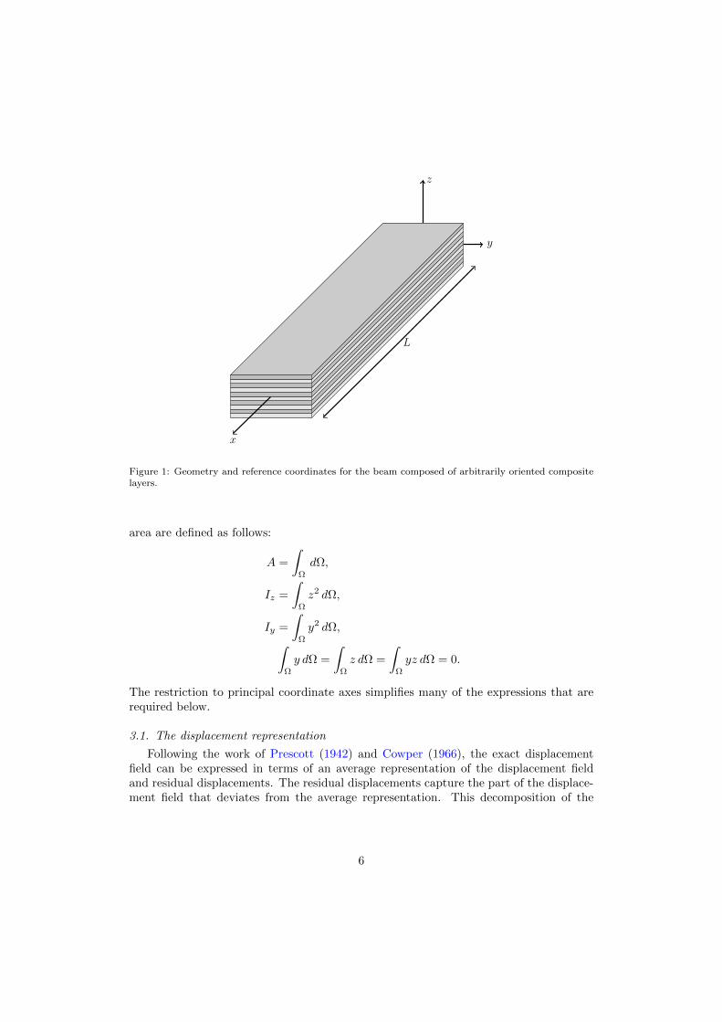
3. The homogenization-based beam theory

We present the theoretical development of the homogenization-based beam theory inthis section. We start with a description of the geometry of the beam under consideration.Next, we develop a kinematic description of the beam using averaged displacement androtation-type variables, based on the work of Prescott (1942) and Cowper (1966). Wethen introduce the fundamental states and use the properties of these solutions to developexpressions for the homogenized stiffness, stress and strain moment correction matrices,and load-dependent corrections. We conclude with a discussion of the benefits of thepresent approach.

The geometry of the beam under consideration is illustrated in Figure 1. The beamis aligned with the x-axis and the geometry and construction of the cross-section do notvary along the length of the beam. In this paper, we are primarily interested in layeredcomposite beams with arbitrarily oriented plies. This type of beam construction resultsin an anisotropic constitutive relationship that exhibits coupling amongst all stress andstrain components. The constitutive equation is expressed as

σ(x, y, z) = C(y, z)ε(x, y, z), (1)

where σ(x, y, z) and ε(x, y, z) are the full states of stress and strain, and C(y, z) is theconstitutive relationship.

The beam of length L is subject to distributed surface tractions applied in the planeperpendicular to the x-axis and is subject to axial forces, bending moments, shear forcesand torques at its ends. Shearing tractions applied on the surface of the beam in the xdirection are excluded from consideration.

The reference axis is located at the geometric centroid of the section and the coordi-nate axes are aligned with the principal axes of the section. As a result, the moments of

5

y

z

x

L

Figure 1: Geometry and reference coordinates for the beam composed of arbitrarily oriented compositelayers.

area are defined as follows:

A =

∫Ω

dΩ,

Iz =

∫Ω

z2 dΩ,

Iy =

∫Ω

y2 dΩ,∫Ω

y dΩ =

∫Ω

z dΩ =

∫Ω

yz dΩ = 0.

The restriction to principal coordinate axes simplifies many of the expressions that arerequired below.

3.1. The displacement representation

Following the work of Prescott (1942) and Cowper (1966), the exact displacementfield can be expressed in terms of an average representation of the displacement fieldand residual displacements. The residual displacements capture the part of the displace-ment field that deviates from the average representation. This decomposition of the

6

displacement field is expressed as

u(x, y, z) =

u(x, y, z)v(x, y, z)w(x, y, z)

=

u0(x) + zuz(x) + yuy(x) + u(x, y, z)v0(x)− zθ(x) + v(x, y, z)w0(x) + yθ(x) + w(x, y, z)

, (2)

where u(x, y, z), and u(x, y, z) =[u v w

]Tare the displacements and residual dis-

placements, respectively. The x-component of the residual displacement u(x, y, z) repre-sents the warping of the section in the axial direction. For convenience, we collect thevariables, u0, v0, θ, uz and uy in a vector u0(x), defined as follows:

u0(x) =[u0 v0 w0 θ uz uy

]T=

∫Ω

[u

A

v

A

w

A

(yw − zv)

Iy + Iz

zu

Iz

yu

Iy

]TdΩ

= L0u(x, y, z).

(3)

Here, u0, v0, and w0 are average displacements in the x, y and z directions. The termsuz, uy and θ are normalized first-order displacement moments about the z, y and xdirections, respectively. Note that uz, uy and θ represent rotation-type variables, but arenot equal to the average rotations of the section. We refer to the vector of variables u0(x)as the normalized displacement moments, since these variables represent zeroth and first-order normalized moments of the displacement field u(x, y, z). In Equation (3), we havealso introduced an operator L0 that takes the full three-dimensional displacement field,u(x, y, z), and returns the normalized moments of displacement. Note that the action ofthis operator removes the y-z dependence of the displacement field.

At this point it should be emphasized that the displacement field decomposition (2)ensures that the normalized displacement moments of the residual displacement field areidentically zero, i.e.,

L0u(x, y, z) = 0.

This property of the residual displacement field will be required later to simplify expres-sions for the strain moments.

The strain produced by the displacements (2) is:

ε(x, y, z) =

εxεyεzγyzγxzγxy

=

u0,x + yuy,x + zuz,z + u,x

v,yw,z

v,z + w,yuz + w0,x + yθ,x + u,z + w,xuy + v0,x − zθ,x + u,y + v,x

, (4)

where the comma convention has been used to denote differentiation. Note that the exactpointwise strain distribution requires knowledge of the residual displacements u(x, y, z).

Instead of using the pointwise strain directly in our theory, we choose to use momentsof the strain distribution. This choice has the advantage that the strain moments aredefined regardless of the through-thickness behavior of the pointwise strain, even whencertain pointwise strain components are discontinuous at material interfaces. It is im-

7

portant to recognize that these interfaces are always parallel to the x direction. As aresult, differentiation with respect to x can commute with integration across the sectionin the regular manner.

The strain moments are defined as follows:

e(x) =[ex κz κy et exz exy

]T=

∫Ω

[εx zεx yεx (yγxz − zγxy) γxz γxy

]TdΩ

= Lsε(x, y, z).

(5)

Here we have introduced another operator Ls that takes the full strain field ε(x, y, z) andreturns the moments of strain e(x).

The next step in the development of the theory is to express the strain moments interms of the displacement representation (2). Using the strain-displacement relation-ships (4), the definitions of the displacement moments (3), and the moments of area, thestrain moments can be written as follows:

e(x) =

Au0,x

Izuz,xIyuy,x

(Iy + Iz) θ,xA (uz + w0,x)A (uy + v0,x)

+ e(x) = ALεu0(x) + e(x), (6)

where e(x) are the moments of the strain produced by the residual displacement. HereA is a diagonal matrix given by

A = diag A, Iz, Iy, (Iy + Iz), A,A .

The operator Lε takes the vector of average displacements and normalized displacementmoments u0(x), such that ALεu0 produces the first term on the right hand side of Equa-tion (6). Note that action of the operator Lε on the normalized displacements, Lεu0(x),produces terms that are identical in form to the center-line strain used in classical Tim-oshenko beam theory. However, the variables u0(x) are interpreted here as normalizeddisplacement moments taken from Equation (3), not as center-line displacements androtations.

The term e(x) in the strain moment expression (6), is a function of the axial residualdisplacement u(x, y, z) and is defined as follows:

e(x) =

∫Ω

u,xzu,xyu,x

y (u,z + w,x)− z (u,y + v,x)u,z + w,xu,y + v,x

dΩ =

∫Ω

000

yu,z − zu,yu,zu,y

dΩ

= Lu(x, y, z),

(7)

8

where the relationship L0u = 0 is used to simplify the expression on the right-handside of the above equation. We have also introduced a linear operator L that takes theresidual axial displacement u(x, y, z) and returns the moments e(x).

The strain moments corresponding to torsion et and shear exz and exy involve termsfrom both the normalized displacement moments and the residual axial displacement,u(x, y, z). These extra terms cannot be evaluated unless u(x, y, z) is known. Our ap-proach is to account for the effect of the residual displacements while formulating thetheory in terms of the average displacement variables, u0(x). The details of this approachare outlined in the following sections.

3.2. The equilibrium equations

The equilibrium equations are formulated based on the classical approach of integrat-ing moments of the three-dimensional equilibrium equations over the cross-section of thebeam. The axial, bending, torsion and shear resultants are defined as follows,

s(x) =[N Mz My T Qz Qy

]T=

∫Ω

[σx zσx yσx (yσxz − zσxy) σxz σxy

]TdΩ

= Lsσ(x, y, z).

(8)

Here, Ls is the same operator that was introduced for the strain moments (5). We referto the variables s(x) as the stress resultants (also known as stress moments). Integratingmoments of the three-dimensional equilibrium equations over the section results in thefollowing equilibrium equations:

N,xMy,x −QzMz,x −Qy

T,xQy,xQz,x

+

000PxPyPz

= 0. (9)

The torque Px(x) and forces Py(x) and Pz(x) are defined as follows:

Px(x) =

∫S

ytz − zty dS,

Py(x) =

∫S

ty dS,

Pz(x) =

∫S

tz dS,

(10)

where ty and tz are the y and z components of the surface traction. The integrals aboveare carried out over the boundary of the cross-section S.

3.3. The fundamental states

In this section we present a decomposition of the stress and strain distribution withinthe beam. This stress and strain decomposition is based on a linear combination of

9

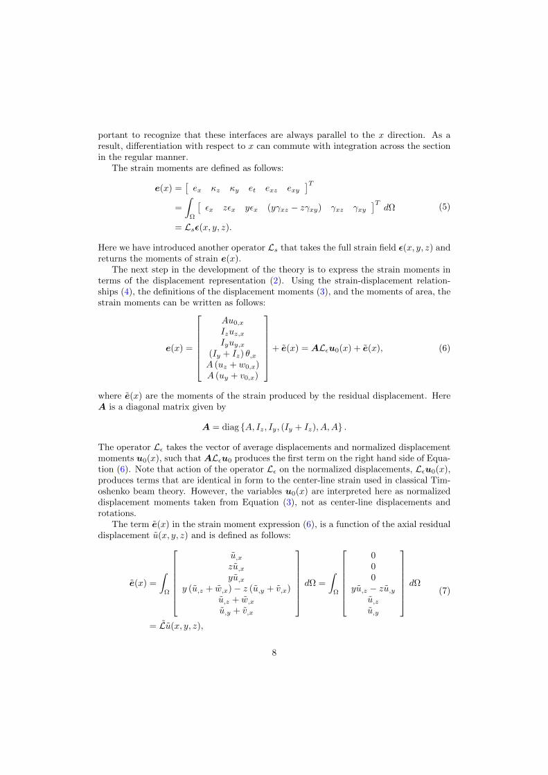
axially-invariant stress and strain solutions that we call the fundamental states. Theuse of the fundamental states leads to a consistent method for deriving the constitutiverelationship between the stress resultants and the strain moments. Furthermore, the fun-damental states can be used to reconstruct the approximate stress and strain distributionin the beam in a post-processing step. Our representation of the solution is similar to thestress representation presented by Ladeveze and Simmonds (1998) and used by El Fatmi(2007a,b), however, unlike these authors, we also use an analogous representation of thestrain solution that is later used to construct the homogenized stiffness relationship. Inthis section we describe the properties of the fundamental states and how they are usedin the present theory.

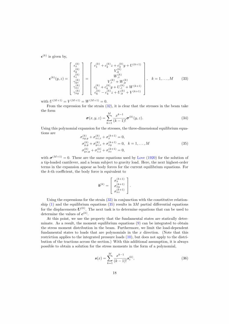
Primary fundamental states Stress resultants

xy

z

First N = 1

Second Mz = 1

Third My = 1

Fourth T = 1

Fifth Qz = 1 Mz = x

Sixth Qy = 1 My = x

Load-dependent fundamental state

FirstPz = 1 Qz = −x

Mz = −x2/2

Figure 2: An illustration of the primary fundamental states and the distribution of the stress resultants.Forces are denoted by a single arrow and moments by a double arrow.

The fundamental states are the axially-invariant, or x-independent, stress and strainsolutions. These solutions are obtained from specially-chosen, statically determinatebeam problems. The loading conditions leading to the fundamental states are shown inFigure 2. These beam problems are sometimes referred to as the Saint–Venant prob-

10

lem (Iesan, 1986a), for axial, bending, torsion, and shear loads, and the Almansi–Michellproblem (Iesan, 1986b), for a beam subject to a distributed surface load. The beam usedto calculate the fundamental states has the same cross-section and construction as thebeam under consideration, but must be long enough that the end effects do not alter thesolution at the mid-plane of the beam. The fundamental states are extracted from thesesolutions by taking the distribution of stress and strain at the mid-plane of the beam.As a result, the fundamental state stress and strain distributions are solutions in the y-zand have no x-dependence.

We distinguish between two types of fundamental state solutions: primary funda-

mental states, which we label σ(k)F (y, z) and ε

(k)F (y, z), and load-dependent fundamental

states, which we label σ(k)LF (y, z) and ε

(k)LF (y, z). The six primary fundamental states

correspond to axial resultant, bending moments about the y and z axes, torsion, andshear in the z and y directions, respectively. The load-dependent fundamental states areassociated with loads applied to the beam. The fundamental states are used here to forman approximation of the stress and strain field within the beam. To complete the stressand strain representation, we also introduce stress and strain residuals, σ(x, y, z) andε(x, y, z), that account for the discrepancy between the approximate stress and strainrepresentation and the exact distribution.

Using these definitions, the stress and strain in the beam may be expressed as follows:

σ(x, y, z) =

6∑k=1

sk(x)σ(k)F (y, z) +

N∑k=1

Pk(x)σ(k)FL(y, z) + σ(x, y, z), (11a)

ε(x, y, z) =

6∑k=1

sk(x)ε(k)F (y, z) +

N∑k=1

Pk(x)ε(k)FL(y, z) + ε(x, y, z). (11b)

The magnitudes of the primary fundamental states are given by the components of thevector s(x) and represent axial force, bending moments, torsion, and shear resultants. In-dividual components of s(x) are written as sk(x). The magnitudes of the load-dependentfundamental states Pk(x) are known from the loading conditions. The fundamental statemagnitudes link the stress and strain distribution.

For consistency between the stress resultants and the stress distribution, the primaryfundamental states must satisfy the relationship,

Lsσ(k)F (y, z) = ik, k = 1, . . . , 6, (12)

where ik is the k-th Cartesian basis vector. This relationship ensures that the stressresultants of the stress distribution (11a) are equal to sk(x). Furthermore, the load-dependent fundamental states must satisfy

Lsσ(k)FL(y, z) = 0, k = 1, . . . , N. (13)

The load-dependent fundamental states do not contribute to the stress resultants. Inaddition, the stress moments of the stress residuals must be zero, i.e.,

Lsσ(x, y, z) = 0.

11

An important benefit of the stress and strain distributions (11) is that they cancapture all components of stress and strain. Typically, beam theories retain only afew components of the stress and strain and assume that the remaining componentsare negligible. These neglected components can sometimes be determined using a post-processing integration of the equilibrium equations through the thickness. For compositematerials, however, it can be important to retain all components of stress and strain, sincesingularities can arise at ply interfaces and both strength and stiffness vary significantlybetween material directions (Pagano and Pipes, 1971).

3.4. The constitutive relationship

With these definitions, we are now prepared to derive the relationship between thestress resultants and the strain moments. To do so, we examine the moments of thestrain field (11b). Using the moment operator Ls, the strain moments of Equation (11b)become,

e(x) =

6∑k=1

sk(x)Lsε(k)F (y, z) +

N∑k=1

Pk(x)Lsε(k)FL(y, z) + Lsε(x, y, z). (14)

Note that the strain moments have contributions from all fundamental states and thestrain residuals.

Next, we introduce a square flexibility matrixE whose k-th column contains the strainmoments from the k-th primary fundamental state. The components of the matrix Eare:

E∗k = Lsε(k)(y, z), k = 1, . . . , 6, (15)

where E∗k is the k-th column of the matrix E. Note that the matrix E is constant fora given beam construction and is independent of x.

The contributions to the strain moments from the primary fundamental states arethe product of the matrix E and the primary fundamental state magnitudes s(x). Re-arranging the strain moment relationship (14) and using the flexibility matrix E yields

Es(x) = e(x)−N∑k=1

Pk(x)Lsε(k)FL(y, z)− Lsε(x, y, z). (16)

The stiffness form of the constitutive relationship can be found by inverting the matrixof strain moments D = E−1, to obtain

s(x) = D

(e(x)−

N∑k=1

Pk(x)Lsε(k)FL(y, z)− Lsε(x, y, z)

). (17)

For a section composed of a single isotropic material the relationship between stress andstrain moments simplifies to

D = diag E,E,E,G,G,G .

Equation (17) is exact in the sense that the stress moments can be determined exactlyif the strain moments, load-dependent strain moments and strain residuals ε(x, y, z) are

12

known. Unfortunately, evaluating the strain residuals ε(x, y, z) requires a full three-dimensional solution of the equations of elasticity.

At this point, an assumption must be made about the contribution to the strainmoments from the term Lsε. Since three-dimensional solutions are typically not available,we assume that the contribution from term Lsε is small and can thus be neglected. Thisassumption introduces an error in the predicted strain moments, and as a result, alsointroduces an error in the predicted stress resultants. Typically, the magnitude of Lsεis highest near the ends of the beam where the solution must adjust to satisfy the endconditions. In situations where these disturbed regions require precise modeling, a beamtheory is not appropriate. However, at a sufficient distance from the ends of the beam,the strain representation (11b) is accurate and thus Lsε should be small.

3.5. The stress and strain moment corrections

Next, we seek a relationship between strain moments and the normalized displace-ment moments. We initially limit the analysis to conditions where no external loads areapplied to the beam. Starting from the stiffness form of the constitutive equations (17),and assuming that the strain residual moments are negligible Lsε = 0, the stress mo-ments may be expressed in terms of the normalized displacement moments u0(x) andthe moments of the warping strain e(x) using Equation (6),

s(x) = D (ALεu0(x) + e(x)) . (18)

To proceed, an expression for e(x) must be obtained. Following the arguments pre-sented by Cowper (1966), we argue that this term should be linearly dependent on themagnitudes of the primary fundamental states in regions sufficiently far removed fromend effects or rapidly varying loads. We write this dependence as

e(x) = Es(x) + er, (19)

where E is a flexibility matrix defined below. Here er, is a warping residual term thataccounts for the deviation of the warping moment in disturbed regions of the beam. Werefer to er as the strain correction error.

Using the operator L from Equation (7), the matrix E can be written as

E∗k = Lu(k)F (y, z), k = 1, . . . , 6, (20)

where u(k)F (y, z) is determined from the residual displacement of the k-th primary fun-

damental state. Note that due to the nature of the operator L, the matrix E only hasentries in the last three rows. All other entries in E are zero.

An expression for the stress resultants in terms of the normalized displacement mo-ments can be obtained by using the simplified form of the constitutive relationship (18),and the moments of the strain due to warping (19), yielding

s(x) = (E − E)−1ALεu0(x) + (E − E)−1er. (21)

In the remainder of this section we assume that the strain correction error is negligible,i.e., er = 0.

13

In order to isolate the effect of the terms E we define the strain moment correctionmatrix as follows:

Cs = (I − ED)−1, (22)

such that Equation (21), with er = 0, simplifies to

s(x) = DCsALεu0(x).

Here, the strain moment correction matrix (22) provides a correction to the strain mo-ments predicted from the average displacements that accounts for e(x). Note that thestrain moment correction matrix Cs has a specific structure. The first three rows of Cs

are always equal to the identity matrix, while the last three rows may contain non-zerosin any location due to the definition of the matrix E.

We also define a stress moment correction matrix as follows:

Ks = (I −DE)−1, (23)

such that Equation (21), with er = 0, simplifies to

s(x) = KsDALεu0(x).

The stress moment correction matrix (23) provides a correction to the stress momentsthat accounts for e(x). In general, the stress moment correction matrix Ks is fullypopulated.

In the case of a doubly symmetric, isotropic section, the stress and strain correctionsmatrices are diagonal and equal. In this case, Cs and Ks take the form

Ks = Cs = diag1, 1, 1, kt, kxz, kxy,

where kt = J/(Iy + Iz) is the strain correction associated with torsion, and J is thetorsional rigidity of the section. The shear strain correction factors kxz and kxy areidentical to those obtained by Cowper (1966) and Mason and Herrmann (1968),

kxz =2(1 + ν)Iz

ν

2(Iy − Iz)−

A

Iz

∫Ω

z2y2 + zχz dΩ

kxy =2(1 + ν)Iy

ν

2(Iz − Iy)− A

Iy

∫Ω

z2y2 + yχy dΩ

where χz and χy are classical Saint–Venant flexure functions (Love, 1920).

3.6. The load-dependent corrections

The constitutive relationship (21) derived above explicitly excluded the effect of ex-ternally applied loads. At this point, we derive load-dependent corrections that accountfor the effect of external loads. We start from the flexibility form of the constitutive equa-tions (16), and neglect the moments of the strain residuals, assuming Lsε = 0. These

14

assumptions result in the following expression for the strain moments:

e(x) = Es(x) +

N∑k=1

Pk(x)Lsε(k)FL(y, z). (24)

The next step is to obtain an expression for the strain moments e(x) as a functionof the normalized displacement moments u0(x). The externally applied loads produceadditional moments of the warping strain. In an analogous manner to the primaryfundamental state contributions, we assume that these moments of the warping strainare predicted by the load-dependent fundamental states and are proportional to theapplied load. These assumptions result in the following expression:

e(x) = ALεu0(x) + Es(x) +

N∑k=1

Pk(x)Lu(k)FL(y, z) + er. (25)

Here, u(k)FL(y, z) denotes the warping function associated with the k-th load-dependent

fundamental state and er, is the strain correction error.Again, assuming that er = 0, the flexibility form of the constitutive equations (24) and

the strain moment expression (25) can now be combined into a constitutive relationshipthat takes the following form:

s(x) = (E − E)−1ALεu0(x) +

N∑k=1

Pk(x)s(k)FL, (26)

where the load-dependent stress moment corrections s(k)FL are defined as

s(k)FL = (E − E)−1

(Lu(k)

FL(y, z)− Lsε(k)FL(y, z)

). (27)

In a similar fashion, it can be shown that the strain moments take the modified form

e(x) = CsALεu0 +

N∑k=1

Pk(x)e(k)FL, (28)

where the load-dependent strain moment corrections e(k)FL are defined as

e(k)FL = Cs

(Lu(k)

FL(y, z)− Lsε(k)FL(y, z)

)+ Lsε(k)

FL(y, z). (29)

The load-dependent stress moment corrections (27) and the load-dependent strainmoment corrections (29) take into account the change in the relationship between thestress and strain moments and the normalized displacement moments as a result ofexternally applied loads. The externally applied loads do not directly produce stressmoments; rather, these loads produce strain moments that must be taken into accountin the constitutive relationship (26). The main assumptions required for the derivationof the constitutive expression are that the moments of the strain residuals, Lsε, and the

15

strain moment correction, er, can be neglected. These assumptions are examined belowin the numerical results section.

3.7. The asymmetry of the constitutive relationship

In general, the homogenized stiffness matrix D, and the matrix product DCsA arenot symmetric. This is not a classical result and deserves attention. Linear constitu-tive relationships between pointwise stress and pointwise strain expressed in the formof Equation (1) are symmetric due to the existence of the strain energy density. How-ever, the homogenized stiffness matrix D that relates the stress resultants to the strainmoments cannot be derived from a strain energy density, sinceD relates integrated quan-tities. The integral of the pointwise strain energy density across the section cannot berelated directly to the product of the integrals of stress and strain. As a result, D is notguaranteed to be symmetric. The matrix product DCsA that relates the normalizeddisplacement moments to the stress resultants is not symmetric for the same reason.Within the context of a finite-element implementation of the present beam theory, caremust be taken to ensure that symmetry of the constitutive relationship is not assumed.

4. A finite-element method for the determination of the fundamental states

The fundamental states play an important role within the beam theory presentedin the previous section. In principle, full three-dimensional solutions for each of thefundamental states are required before any analysis can be performed. It is possibleto obtain some exact solutions to the fundamental states, as shown in Kennedy et al.(2011). However, we anticipate that it is only possible to obtain these exact solutionsfor a small set of geometries and beam constructions of interest. In order to solve moregeneral problems, we have develop a finite-element method for the determination of thefundamental states for cross-sections of arbitrary geometry and construction.

It is possible to use conventional three-dimensional finite-elements to obtain the fun-damental state solutions; however, this approach is computationally expensive due to thelarge, three-dimensional mesh requirements. Instead, we develop a technique that onlyrequires computations in the plane of the section, eliminating the need to discretize theaxial direction. This approach is possible due to the fact that the fundamental states arefar-field solutions.

In developing the following finite-element method, we follow the work of Pipes andPagano (1970), who used a semi-inverse approach to obtain the stress and strain distri-butions in a long beam subject to an axial load. We modify the form of the assumeddisplacement field proposed by Pipes and Pagano (1970), but retain the terms that ac-count for the effects of axial force, bending, shear, and torsion. El Fatmi and Zenzri(2002) developed a similar technique to obtain the Saint–Venant and Almansi–Michellsolutions based on the work of Ladeveze and Simmonds (1998). Dong et al. (2001) de-veloped a finite-element solution technique for the Saint–Venant problem based on thework of Iesan (1986a).

In the following section, all variables refer to a single fundamental state calculation.Relationships with the beam theory are described explicitly in Section 4.2. In this finite-element approach, we develop a displacement-based solution to the three-dimensional

16

equations of elasticity based on the following expansion of the displacement field in theaxial direction:

u(x, y, z) =

M∑k=1

xk

k!

(c(k)1 + c

(k)2 z + c

(k)3 y

)+

xk−1

(k − 1)!U (k)(y, z)

,

v(x, y, z) =

M∑k=1

xk

k!

(c(k)6 − c(k)

4 z − c(k)3

x

k + 1

)+

xk−1

(k − 1)!V (k)(y, z)

,

w(x, y, z) =

M∑k=1

xk

k!

(c(k)5 + c

(k)4 y − c(k)

2

x

k + 1

)+

xk−1

(k − 1)!W (k)(y, z)

,

(30)

where the displacements U (k)(y, z), V (k)(y, z) and W (k)(y, z) are written as U (k) =[U (k) V (k) W (k)

]T, and are only functions of y and z. The terms c

(k)1 through c

(k)6

are constant across the section, and we refer to these as the invariants. It is convenient to

collect c(k)1 through c

(k)6 into a vector denoted c(k) =

[c(k)1 . . . c

(k)6

]T. The number of

terms M , retained in the expansion is discussed in more detail below. Pipes and Pagano(1970) used a similar form of Equation (30) with M = 1 to determine the stresses inthe vicinity of the free edge of a laminated composite beam subjected to an axial force.As we demonstrate below, the displacement field above can also be used to predict thestress and strain fields due to bending, torsion, shear, and applied loads.

When M > 1, the representation of the displacement field (30) is not unique. The

invariants c(k)1 through c

(k)6 define displacements that can be represented by U (k+1),

V (k+1) and W (k+1). Furthermore, displacement boundary conditions must be imposedon the displacement field (30) to remove rigid body translation and rotation modes. Inorder to handle both of these issues, we impose the constraint

L0U(k)(y, z) = 0, k = 1, . . . ,M, (31)

where L0 is the operator defined in (3). This constraint removes the rigid body translationand rotation modes for k = 1, and ensures that the displacements are uniquely definedfor k > 1. A different method for imposing the boundary conditions could be applied,but we have found that Equation (31) simplifies later results in relation to the beamtheory.

The strain produced by the displacement field (30) is most clearly expressed in theform,

ε(x, y, z) =

M∑k=1

xk−1

(k − 1)!ε(k)(y, z), (32)

where ε(k)(y, z) is a strain distribution in the y-z plane. In Equation (32), the coefficient

17

ε(k) is given by,

ε(k)(y, z) =

ε(k)x

ε(k)y

ε(k)z

γ(k)yz

γ(k)xz

γ(k)xy

=

c(k)1 + c

(k)2 z + c

(k)3 y + U (k+1)

V(k),y

W(k),z

V(k),z +W

(k),y

c(k)5 + c

(k)4 y + U

(k),z +W (k+1)

c(k)6 − c(k)

4 z + U(k),y + V (k+1)

, k = 1, . . . ,M (33)

with U (M+1) = V (M+1) = W (M+1) = 0.From the expression for the strain (32), it is clear that the stresses in the beam take

the form

σ(x, y, z) =

M∑k=1

xk−1

(k − 1)!σ(k)(y, z). (34)

Using this polynomial expansion for the stresses, the three-dimensional equilibrium equa-tions are

σ(k)xy,y + σ(k)

xz,z + σ(k+1)x = 0,

σ(k)y,y + σ(k)

yz,z + σ(k+1)xy = 0,

σ(k)yz,y + σ(k)

z,z + σ(k+1)xz = 0,

k = 1, . . . ,M (35)

with σ(M+1) = 0. These are the same equations used by Love (1920) for the solution ofa tip-loaded cantilever, and a beam subject to gravity load. Here, the next highest-orderterms in the expansion appear as body forces for the current equilibrium equations. Forthe k-th coefficient, the body force is equivalent to

b(k) =

σ(k+1)x

σ(k+1)xy

σ(k+1)xz

.Using the expressions for the strain (33) in conjunction with the constitutive relation-

ship (1) and the equilibrium equations (35) results in 3M partial differential equations

for the displacements U (k). The next task is to determine equations that can be used todetermine the values of c(k).

At this point, we use the property that the fundamental states are statically deter-minate. As a result, the moment equilibrium equations (9) can be integrated to obtainthe stress moment distribution in the beam. Furthermore, we limit the load-dependentfundamental states to loads that are polynomials in the x direction. (Note that thisrestriction applies to the integrated pressure loads (10), but does not apply to the distri-bution of the tractions across the section.) With this additional assumption, it is alwayspossible to obtain a solution for the stress moments in the form of a polynomial,

s(x) =

M∑k=1

xk−1

(k − 1)!s(k)c , (36)

18

where s(k)c is the k-th coefficient in the polynomial. Clearly, the value of M must be

chosen such that M − 1 is equal to the degree of the polynomial stress-moment distri-bution (36). The primary fundamental states corresponding to axial force, torsion andbending moments can be determined with M = 1. The primary fundamental states cor-responding to shear require a solution with M = 2 corresponding to a linearly varyingbending moment and constant shear. The load-dependent fundamental state correspond-ing to a distributed surface loads requires M = 3, with a quadratically varying bendingmoment and linearly varying shear.

For the moments of the stress expansion (34) to match the coefficients of the stressmoment polynomial (36), we impose the additional constraint,

Lsσ(k)(y, z) = s(k)c , k = 1, . . . ,M. (37)

These constraints represent an additional 6M equations that are used to determine c(k).To summarize, there are 3M , U (k)(y, z) coefficients defined in the y-z plane, and an

additional 6M constants c(k) that are required in the displacement field (30). These vari-ables can be determined from the 6M moment constraints (37) and the 3M equilibriumequations (35) used in conjunction with the strain expressions (33) and the constitutiverelationship (1).

It is important to note that this system of equations can be solved in a sequentialfashion. The coefficients of the highest order k = M , U (M), and c(M), are independentof the lower order coefficients k < M . The k = M terms couple with the next terms, k =M −1, U (M−1), and c(M−1), through the equivalent body-force terms in the equilibriumequations (35). This sequential process continues until all the coefficients, U (k), andc(k), have been determined. This same solution technique was used by Love (1920) forisotropic beams.

4.1. Finite-element implementation

We use a straightforward finite-element implementation of the above equations. Thisimplementation shares many similarities with the approach of Dong et al. (2001). Herewe pose our problem in terms of the displacement of the beam under the action of a pre-scribed load. Dong et al. (2001) seeks a solution in two steps: first obtaining the distribu-tion of the warping displacements for axial, bending, torsion, and shear, then obtainingthe amplitudes of the Saint–Venant solution in a second calculation. Here we employconventional isoparametric displacement-based elements with bi-cubic Lagrangian shapefunctions in the plane for the 3M displacement field componentsU (k)(y, z), k = 1, . . . ,M .

We write the nodal displacements of U (k)(y, z) in the vector d(k). It can be shown thatthe constraints on the stress moments (37) arise naturally using the principle of sta-tionary total potential energy. We impose the unconventional displacement boundaryconditions (31) by adding Lagrange multipliers and employ a Gauss quadrature approxi-mation of the constraint (31). The discrete form of the displacement constraint is writtenas

L0d(k) = 0,

where L0 is the discrete analogue of L0. We denote the Lagrange multipliers associatedwith the displacement constraints as λ(k).

19

The discrete approximation of the k-th coefficient of the strain expansion (33) iswritten as

ε(k) = Bd(k)e +Bcc

(k) +Bud(k+1)e ,

where B, Bc and Bu take the nodal k-th displacements, k-th invariants and k + 1-thdisplacement and produce the pointwise strain. Here, the subscript e has been used todenote the element displacements from the vector d(k). The matrices B and Bu aredefined as follows:

B =

0 0 0 . . .0 N1,y 0 . . .0 0 N1,z . . .0 N1,z N1,y . . .

N1,z 0 0 . . .N1,y 0 0 . . .

, Bu =

N1 0 0 . . .0 0 0 . . .0 0 0 . . .0 0 0 . . .0 0 N1 . . .0 N1 0 . . .

,

where Ni are the shape functions, and the comma notation has been used for differenti-ation. The pattern in the matrices B and Bu, repeats itself for each node. The matrixBc is given by

Bc =

1 z y 0 0 00 0 0 0 0 00 0 0 0 0 00 0 0 0 0 00 0 0 y 1 00 0 0 −z 0 1

.

For convenience, we introduce the element matrices in a block matrix form as follows: Kedd

Kecd Ke

cc

Keud Ke

uc Keuu

=

∫Ωe

BTCB

BTc CB BT

c CBc

BTuCB BT

uCBc BTuCBu

dΩe, (38)

where Ωe is the element domain. The element matrices are denoted with a superscripte. The superscript e is omitted for the assembled form of the matrix.

The assembled finite-element equations are: Kdd KTcd LT0

Kcd Kcc 0L0 0 0

d(k)

c(k)

λ(k)

=

f (k)

f (k)c

0

. (39)

Care must be exercised when solving equation (39), since the matrix Kdd is singular.This is due to the fact that no conventional Dirichlet boundary conditions are applied toKdd. However, the final row of the system of equations (39) imposes a constraint thatremoves this singularity.

The two terms on the right hand side of Equation (39) are

f (k) = f (k)s + f

(k)b −KT

udd(k+1),

f (k)c = s(k)

c −KTucd

(k+1),(40)

20

where terms with superscripts greater than M are zero. The term fs is the surfacetraction contribution to the right hand side and f c is the right hand side for the invariants.

The force vector, f(k)b , represents a body force associated with the k+ 1-th fundamental

state, defined as follows:

f(k)b = Kudd

(k+1) +Kucc(k+1) +Kuud

(k+2).

Note that the left hand side of Equation (39) is the same for each coefficient k. Therefore,only the right hand sides (40) needs to be recomputed in each subsequent solution.

4.2. Relation to beam theory

In this section we outline the connection between the finite-element approach de-scribed above and the proposed beam theory.

The computations outlined above are performed for each fundamental state. First,the polynomial stress resultant coefficients from Equation (36) are determined. Thesepolynomials are summarized for each of the fundamental states in Figure 2. Next, the un-knowns d(k) and c(k), k = 1 . . .M , are determined using Equation (39). The fundamentalstate stress and strain solutions are the lowest-order terms of the polynomial expressionsfor the stress in Equations (34) and (32), respectively. Therefore, the fundamental statesare σ(1)(y,z) and ε(1)(y, z) in the y-z plane.

With this definition, the strain moments of the fundamental state can be computedusing

e = Lsε(1)(y, z), (41)

where Ls is a discrete analogue of the operator Ls computed using Gaussian quadra-ture. The strain moments are required to compute the flexibility matrix E (15) andfor components of the stress and strain moment corrections in Equations (27) and (29),respectively.

Another key quantity required for the beam theory is the axial warping u(x, y, z). Thex-independent component of axial warping is precisely U (1)(y, z) due to the impositionof the displacement moment constraint (31). The moments of the warping strain can beevaluated using:

e = LU (1)(y, z), (42)

where L is the discrete analogue of L and is computed using Gaussian quadrature. Theterms e are required for computing the flexibility matrix E (20), and the stress andstrain moment correction matrices Ks (23) and Cs (22), respectively.

5. Results

In this section we present results using the finite-element approach presented in Sec-tion 4, and demonstrate the modeling capabilities of the beam theory. This section isdivided into three parts. In the first part we compare the present beam theory results toresults obtained by Cowper (1966) for rectangular and hollow cylindrical isotropic sec-tions, and results obtained by Kennedy et al. (2011) for isotropic and layered isotropicsections. In the second part we compare the beam theory to full three-dimensional finite-element results. In the last part we present a parameter study to explore the behavior of

21

the homogenized stiffness and the strain moment correction matrix Cs for an angle-plylaminate.

C

a

b rb

Pt = 4/5

Pb = 1/5

E

αE

E

(a) Three layer section

C

a

b

b/4

θ1

θ2

θ3

θ4

(b) Rectangular section

C

2a

2b

(c) Hollow cylinder

Cr

ba

a

Pz = 1

θ1θ2θ3θ4

(d) Angle section

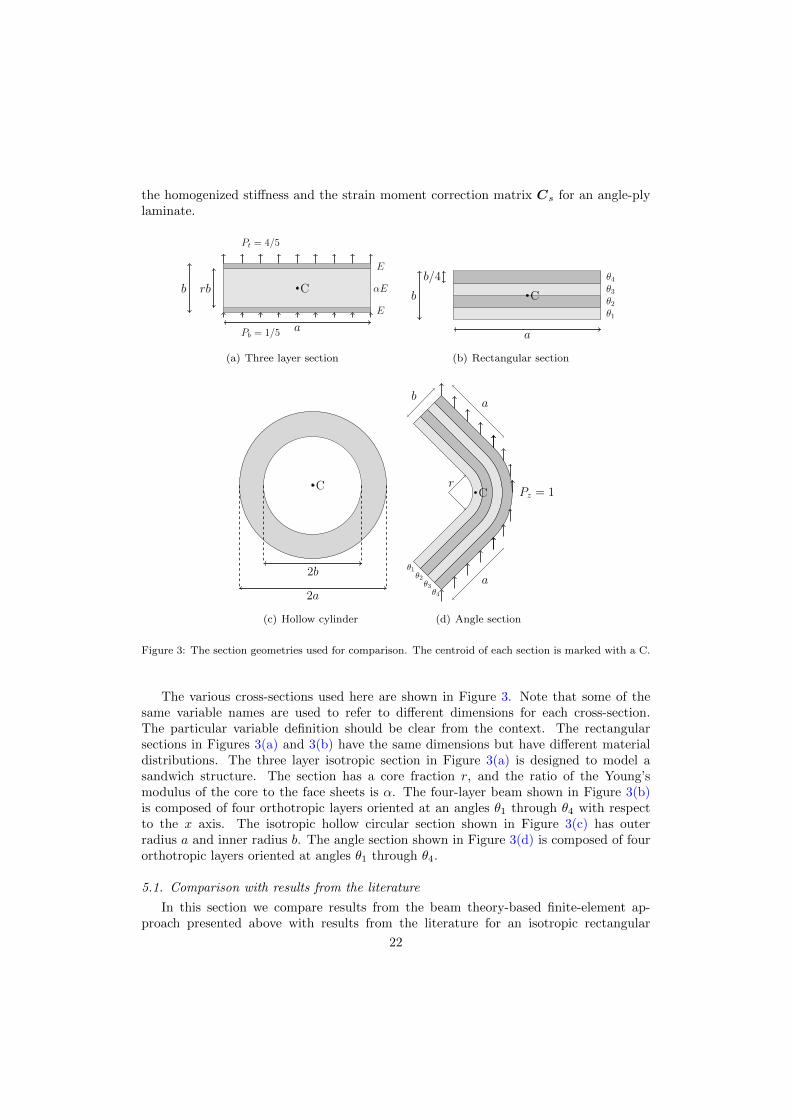
Figure 3: The section geometries used for comparison. The centroid of each section is marked with a C.

The various cross-sections used here are shown in Figure 3. Note that some of thesame variable names are used to refer to different dimensions for each cross-section.The particular variable definition should be clear from the context. The rectangularsections in Figures 3(a) and 3(b) have the same dimensions but have different materialdistributions. The three layer isotropic section in Figure 3(a) is designed to model asandwich structure. The section has a core fraction r, and the ratio of the Young’smodulus of the core to the face sheets is α. The four-layer beam shown in Figure 3(b)is composed of four orthotropic layers oriented at an angles θ1 through θ4 with respectto the x axis. The isotropic hollow circular section shown in Figure 3(c) has outerradius a and inner radius b. The angle section shown in Figure 3(d) is composed of fourorthotropic layers oriented at angles θ1 through θ4.

5.1. Comparison with results from the literature

In this section we compare results from the beam theory-based finite-element ap-proach presented above with results from the literature for an isotropic rectangular

22

section, the hollow isotropic circular section (Figure 3(c)) and the three layer section(Figure 3(a)).

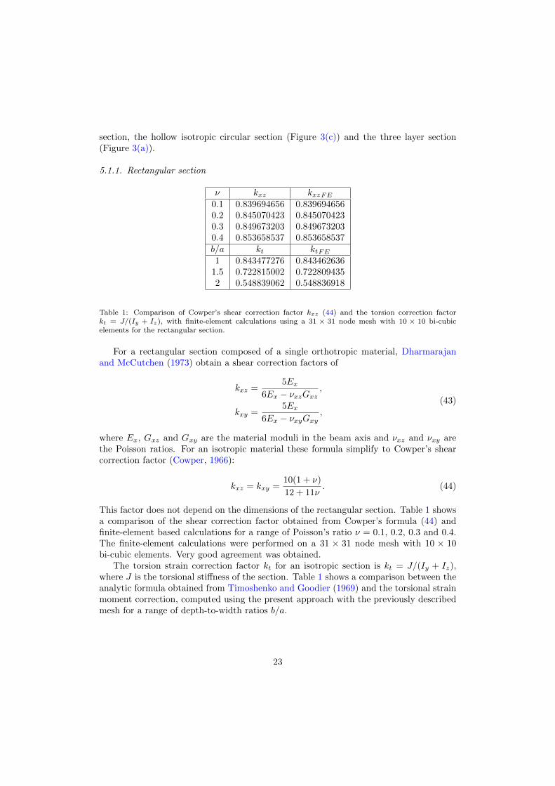
5.1.1. Rectangular section

ν kxz kxzFE0.1 0.839694656 0.8396946560.2 0.845070423 0.8450704230.3 0.849673203 0.8496732030.4 0.853658537 0.853658537b/a kt ktFE1 0.843477276 0.843462636

1.5 0.722815002 0.7228094352 0.548839062 0.548836918

Table 1: Comparison of Cowper’s shear correction factor kxz (44) and the torsion correction factorkt = J/(Iy + Iz), with finite-element calculations using a 31 × 31 node mesh with 10 × 10 bi-cubicelements for the rectangular section.

For a rectangular section composed of a single orthotropic material, Dharmarajanand McCutchen (1973) obtain a shear correction factors of

kxz =5Ex

6Ex − νxzGxz,

kxy =5Ex

6Ex − νxyGxy,

(43)

where Ex, Gxz and Gxy are the material moduli in the beam axis and νxz and νxy arethe Poisson ratios. For an isotropic material these formula simplify to Cowper’s shearcorrection factor (Cowper, 1966):

kxz = kxy =10(1 + ν)

12 + 11ν. (44)

This factor does not depend on the dimensions of the rectangular section. Table 1 showsa comparison of the shear correction factor obtained from Cowper’s formula (44) andfinite-element based calculations for a range of Poisson’s ratio ν = 0.1, 0.2, 0.3 and 0.4.The finite-element calculations were performed on a 31 × 31 node mesh with 10 × 10bi-cubic elements. Very good agreement was obtained.

The torsion strain correction factor kt for an isotropic section is kt = J/(Iy + Iz),where J is the torsional stiffness of the section. Table 1 shows a comparison between theanalytic formula obtained from Timoshenko and Goodier (1969) and the torsional strainmoment correction, computed using the present approach with the previously describedmesh for a range of depth-to-width ratios b/a.

23

b/a kxz kxzFE0.75 0.547851299 0.5478512990.25 0.771774856 0.7717761700.15 0.837998917 0.838010143

Table 2: Comparison of Cowper’s shear correction factor for a hollow cylinder with the present approachfor a series of radius ratios. Finite-element calculations were performed on a 120 × 16 node mesh with40× 5 bi-cubic elements.

r kxz kxzFE MP MPFE

0.25 0.714966088 0.714966088 1.385478992 1.385541640.5 0.744974670 0.744974670 3.041345731 3.041391930.75 0.825732040 0.825732040 2.767575511 2.76760868

Table 3: Comparison of the shear correction factor and stress moment correction for the isotropic threelayer beam for a case with α = 0.1

5.1.2. Hollow circular section

For a hollow, circular section, Cowper (1966) obtained a shear correction value of

kxz =6(1 + ν)(1 +m2)2

(7 + 6ν)(1 +m2)2 + (20 + 12ν)m2, (45)

where m = b/a is the ratio of the inner to the outer radius. The geometry of thehollow section is shown in Figure 3(c). Table 2 shows a comparison between Cowper’sformula (45) and finite-element calculations performed on a 120 × 16 node mesh with40× 5 bi-cubic elements.

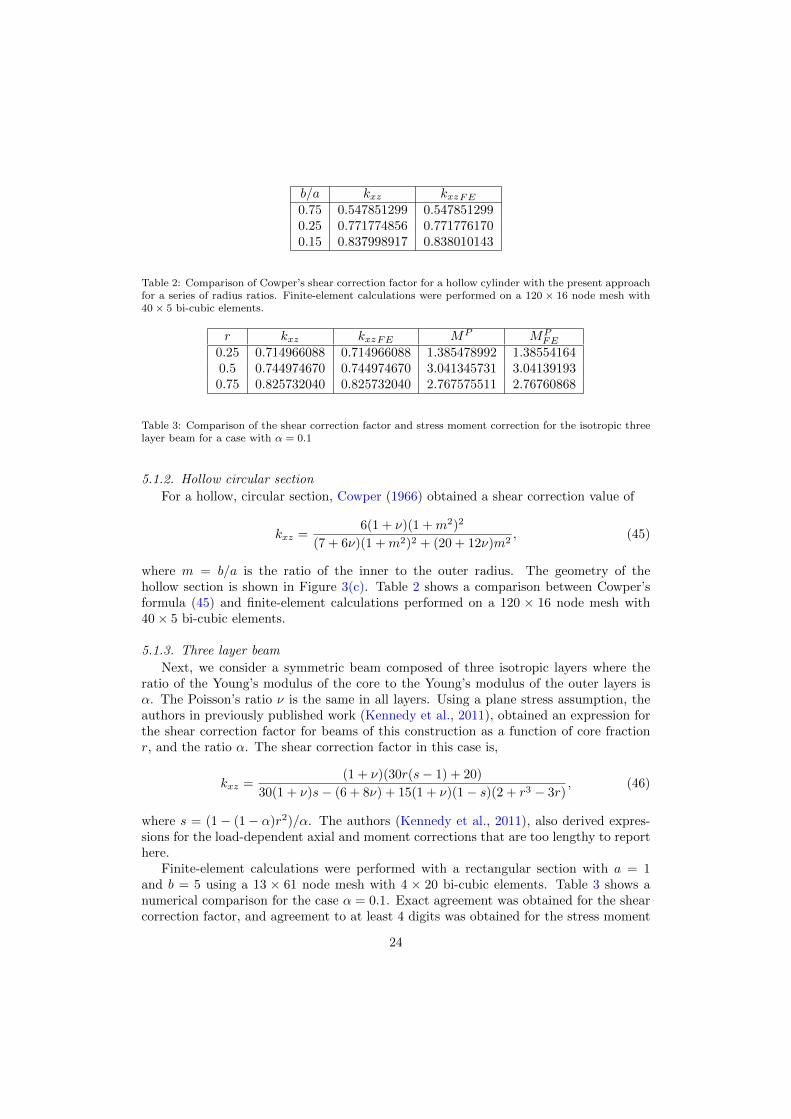
5.1.3. Three layer beam

Next, we consider a symmetric beam composed of three isotropic layers where theratio of the Young’s modulus of the core to the Young’s modulus of the outer layers isα. The Poisson’s ratio ν is the same in all layers. Using a plane stress assumption, theauthors in previously published work (Kennedy et al., 2011), obtained an expression forthe shear correction factor for beams of this construction as a function of core fractionr, and the ratio α. The shear correction factor in this case is,

kxz =(1 + ν)(30r(s− 1) + 20)

30(1 + ν)s− (6 + 8ν) + 15(1 + ν)(1− s)(2 + r3 − 3r), (46)

where s = (1− (1− α)r2)/α. The authors (Kennedy et al., 2011), also derived expres-sions for the load-dependent axial and moment corrections that are too lengthy to reporthere.

Finite-element calculations were performed with a rectangular section with a = 1and b = 5 using a 13 × 61 node mesh with 4 × 20 bi-cubic elements. Table 3 shows anumerical comparison for the case α = 0.1. Exact agreement was obtained for the shearcorrection factor, and agreement to at least 4 digits was obtained for the stress moment

24

Core fraction: r

Shearstrain

correction:k

0 0.2 0.4 0.6 0.8 1

0.7

0.75

0.8

0.85

0.9

0.95present α = 0.5

present α = 0.1

present α = 0.01

α = 0.5

α = 0.1

α = 0.01

Figure 4: Comparison of the shear correction factor for the isotropic three layer beam. Finite-elementresults from the present approach are compared with Equation (46).

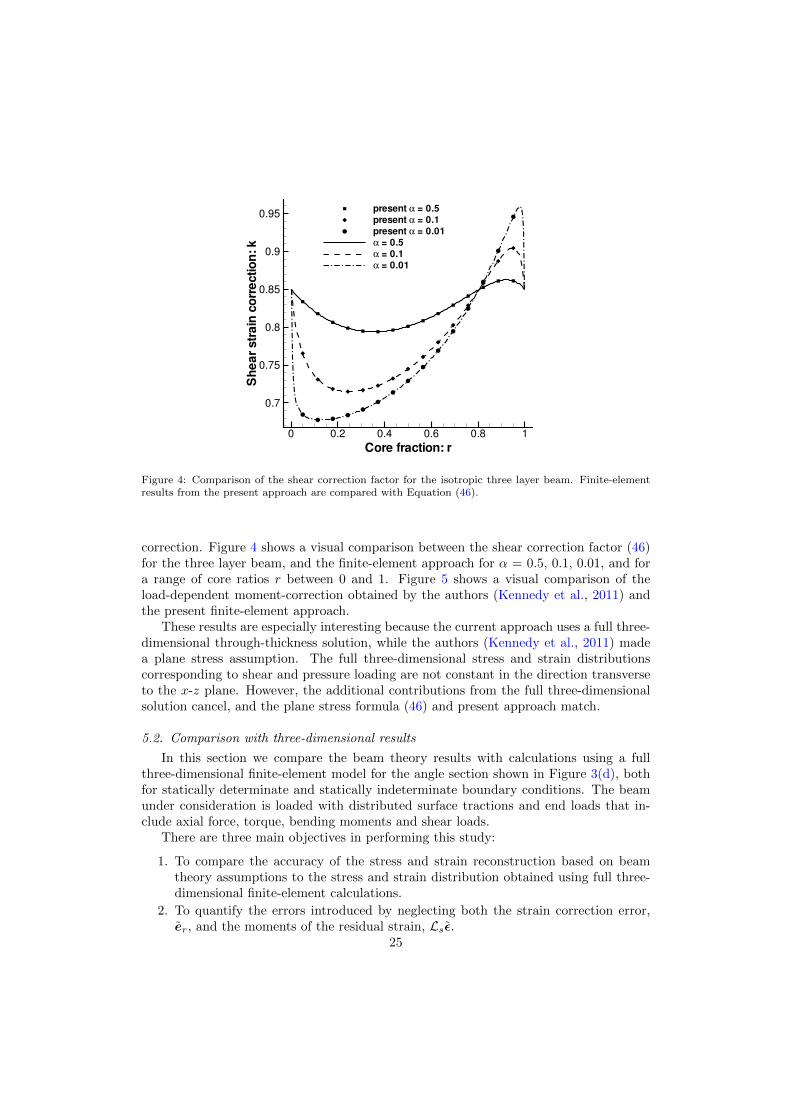
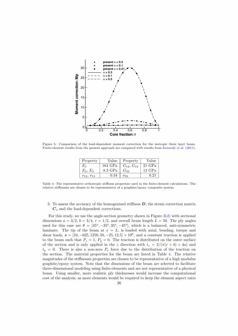
correction. Figure 4 shows a visual comparison between the shear correction factor (46)for the three layer beam, and the finite-element approach for α = 0.5, 0.1, 0.01, and fora range of core ratios r between 0 and 1. Figure 5 shows a visual comparison of theload-dependent moment-correction obtained by the authors (Kennedy et al., 2011) andthe present finite-element approach.

These results are especially interesting because the current approach uses a full three-dimensional through-thickness solution, while the authors (Kennedy et al., 2011) madea plane stress assumption. The full three-dimensional stress and strain distributionscorresponding to shear and pressure loading are not constant in the direction transverseto the x-z plane. However, the additional contributions from the full three-dimensionalsolution cancel, and the plane stress formula (46) and present approach match.

5.2. Comparison with three-dimensional results

In this section we compare the beam theory results with calculations using a fullthree-dimensional finite-element model for the angle section shown in Figure 3(d), bothfor statically determinate and statically indeterminate boundary conditions. The beamunder consideration is loaded with distributed surface tractions and end loads that in-clude axial force, torque, bending moments and shear loads.

There are three main objectives in performing this study:

1. To compare the accuracy of the stress and strain reconstruction based on beamtheory assumptions to the stress and strain distribution obtained using full three-dimensional finite-element calculations.

2. To quantify the errors introduced by neglecting both the strain correction error,er, and the moments of the residual strain, Lsε.

25

Core fraction: r

Momentcorrection:Mp

0 0.2 0.4 0.6 0.8 1

0

5

10

15

20

25

30

present α = 0.5

present α = 0.1

present α = 0.01

α = 0.5

α = 0.1

α = 0.5

Figure 5: Comparison of the load-dependent moment correction for the isotropic three layer beam.Finite-element results from the present approach are compared with results from Kennedy et al. (2011).

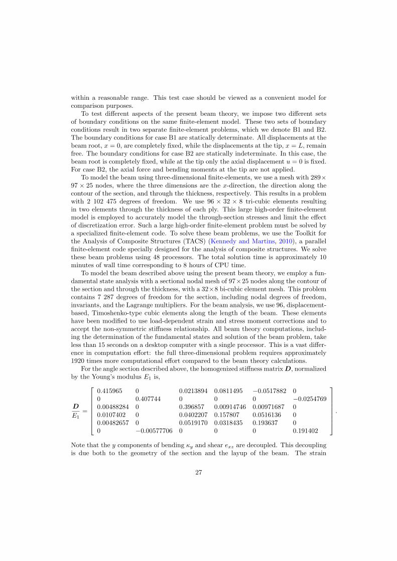
Property Value Property ValueE1 164 GPa G12, G13 21 GPaE2, E3 8.3 GPa G23 12 GPaν12, ν13 0.34 ν23 0.21

Table 4: The representative orthotropic stiffness properties used in the finite-element calculations. Therelative stiffnesses are chosen to be representative of a graphite/epoxy composite system.

3. To assess the accuracy of the homogenized stiffness D, the strain correction matrixCs and the load-dependent corrections.

For this study, we use the angle-section geometry shown in Figure 3(d) with sectionaldimensions a = 3/2, b = 3/4, r = 1/2, and overall beam length L = 50. The ply anglesused for this case are θ = [45o,−35o, 35o,−45o], which is a balanced, anti-symmetriclaminate. The tip of the beam at x = L, is loaded with axial, bending, torque andshear loads, s = [10,−625, 1250, 50,−25, 12.5] × 106, and a constant traction is appliedto the beam such that Pz = 1, Py = 0. The traction is distributed on the outer surfaceof the section and is only applied in the z direction with tz = 2/(π(r + b) + 4a) andty = 0. There is also a non-zero Px force due to the distribution of the traction onthe section. The material properties for the beam are listed in Table 4. The relativemagnitudes of the stiffnesses properties are chosen to be representative of a high modulusgraphite/epoxy system. Note that the dimensions of the beam are selected to facilitatethree-dimensional modeling using finite-elements and are not representative of a physicalbeam. Using smaller, more realistic ply thicknesses would increase the computationalcost of the analysis, as more elements would be required to keep the element aspect ratio

26

within a reasonable range. This test case should be viewed as a convenient model forcomparison purposes.

To test different aspects of the present beam theory, we impose two different setsof boundary conditions on the same finite-element model. These two sets of boundaryconditions result in two separate finite-element problems, which we denote B1 and B2.The boundary conditions for case B1 are statically determinate. All displacements at thebeam root, x = 0, are completely fixed, while the displacements at the tip, x = L, remainfree. The boundary conditions for case B2 are statically indeterminate. In this case, thebeam root is completely fixed, while at the tip only the axial displacement u = 0 is fixed.For case B2, the axial force and bending moments at the tip are not applied.

To model the beam using three-dimensional finite-elements, we use a mesh with 289×97 × 25 nodes, where the three dimensions are the x-direction, the direction along thecontour of the section, and through the thickness, respectively. This results in a problemwith 2 102 475 degrees of freedom. We use 96 × 32 × 8 tri-cubic elements resultingin two elements through the thickness of each ply. This large high-order finite-elementmodel is employed to accurately model the through-section stresses and limit the effectof discretization error. Such a large high-order finite-element problem must be solved bya specialized finite-element code. To solve these beam problems, we use the Toolkit forthe Analysis of Composite Structures (TACS) (Kennedy and Martins, 2010), a parallelfinite-element code specially designed for the analysis of composite structures. We solvethese beam problems using 48 processors. The total solution time is approximately 10minutes of wall time corresponding to 8 hours of CPU time.

To model the beam described above using the present beam theory, we employ a fun-damental state analysis with a sectional nodal mesh of 97×25 nodes along the contour ofthe section and through the thickness, with a 32×8 bi-cubic element mesh. This problemcontains 7 287 degrees of freedom for the section, including nodal degrees of freedom,invariants, and the Lagrange multipliers. For the beam analysis, we use 96, displacement-based, Timoshenko-type cubic elements along the length of the beam. These elementshave been modified to use load-dependent strain and stress moment corrections and toaccept the non-symmetric stiffness relationship. All beam theory computations, includ-ing the determination of the fundamental states and solution of the beam problem, takeless than 15 seconds on a desktop computer with a single processor. This is a vast differ-ence in computation effort: the full three-dimensional problem requires approximately1920 times more computational effort compared to the beam theory calculations.

For the angle section described above, the homogenized stiffness matrixD, normalizedby the Young’s modulus E1 is,

D

E1=

0.415965 0 0.0213894 0.0811495 −0.0517882 00 0.407744 0 0 0 −0.02547690.00488284 0 0.396857 0.00914746 0.00971687 00.0107402 0 0.0402207 0.157807 0.0516136 00.00482657 0 0.0519170 0.0318435 0.193637 00 −0.00577706 0 0 0 0.191402

.

Note that the y components of bending κy and shear exz are decoupled. This decouplingis due both to the geometry of the section and the layup of the beam. The strain

27

correction matrix Cs is,

Cs =

1 0 0 0 0 00 1 0 0 0 00 0 1 0 0 00.0670449 0 −0.0202593 0.399008 0.396402 0−0.0351000 0 −0.0891052 0.311563 0.595588 00 0.00225714 0 0 0 0.542370

.

Note again that there is coupling between the y component of shear and bending andthe z component of shear and torsion.

The strain moment correction e(1)FL and stress-moment correction s

(1)FL are,

e(1)FL =

[0 0 0 0 0 4.47333376× 10−6

]T,

s(1)FL

E1=[

0 7.12433× 10−4 0 0 0 −3.87965× 10−4]T.

While the stress and strain moment corrections are small in magnitude, ignoring theseterms produces measurable errors when the beam theory calculations are compared withfinite-element results.

5.2.1. Statically determinate beam

In this section we examine the results from the problem B1. Since this case is staticallydeterminate, the stress moments can be determined from the equilibrium equations (9)alone. Therefore, the results in this section must be interpreted from the point of viewof known stress resultants, but unknown strain moments.

First, we examine the accuracy of the stress and strain reconstruction from Equa-tion (11). Instead of plotting the error in each of the 12 components of stress and strain,we use the following quantity to concisely present a single error measure per unit lengthof the beam:

∆SErel(x) =

∫Ωε3D · σ3D dΩ∫

Ωε3D · σ3D dΩ

. (47)

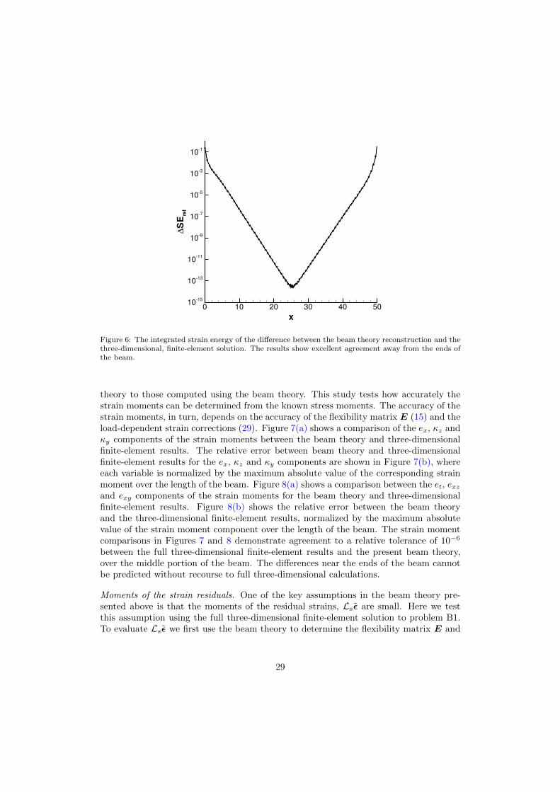
In the above equation, σ3D and ε3D are the stress and strain solutions from the three-dimensional finite-element problem, while σ3D and ε3D are the differences between thethree-dimensional solution and the beam theory reconstruction, and therefore representapproximations of the true stress and strain residuals, σ and ε, in Equation (11). Thequantity ∆SErel is the strain energy of the difference between the beam theory and thefull three-dimensional solution, per unit length of the beam, normalized by the sectionalstrain energy at the current x position. An error in one component of the stress andstrain produces a measurable error in ∆SErel. As a result, ∆SErel shows the accuracy ofall components of the stress and strain reconstruction.

Figure 6 shows ∆SErel as a function of x-location for the case B1. ∆SErel is largest atthe ends of the beam and decreases rapidly towards the center of the beam. This resultdemonstrates the high degree of accuracy of the stress and strain reconstruction just afew thicknesses away from the ends of the beam.

Next, we compare the strain moments computed from the full three-dimensional

28

x

∆SE

rel

0 10 20 30 40 5010

­15

10­13

10­11

10­9

10­7

10­5

10­3

10­1

Figure 6: The integrated strain energy of the difference between the beam theory reconstruction and thethree-dimensional, finite-element solution. The results show excellent agreement away from the ends ofthe beam.

theory to those computed using the beam theory. This study tests how accurately thestrain moments can be determined from the known stress moments. The accuracy of thestrain moments, in turn, depends on the accuracy of the flexibility matrix E (15) and theload-dependent strain corrections (29). Figure 7(a) shows a comparison of the ex, κz andκy components of the strain moments between the beam theory and three-dimensionalfinite-element results. The relative error between beam theory and three-dimensionalfinite-element results for the ex, κz and κy components are shown in Figure 7(b), whereeach variable is normalized by the maximum absolute value of the corresponding strainmoment over the length of the beam. Figure 8(a) shows a comparison between the et, exzand exy components of the strain moments for the beam theory and three-dimensionalfinite-element results. Figure 8(b) shows the relative error between the beam theoryand the three-dimensional finite-element results, normalized by the maximum absolutevalue of the strain moment component over the length of the beam. The strain momentcomparisons in Figures 7 and 8 demonstrate agreement to a relative tolerance of 10−6

between the full three-dimensional finite-element results and the present beam theory,over the middle portion of the beam. The differences near the ends of the beam cannotbe predicted without recourse to full three-dimensional calculations.

Moments of the strain residuals. One of the key assumptions in the beam theory pre-sented above is that the moments of the residual strains, Lsε are small. Here we testthis assumption using the full three-dimensional finite-element solution to problem B1.To evaluate Lsε we first use the beam theory to determine the flexibility matrix E and

29

the strain moment contributions from the externally applied loads:

eP = PzLsε(1)FL(y, z),

where Pz = 1 is the magnitude of the applied load and Ls is the discrete analogue of Ls.Based on Equation (16), the discrete analogue of Lsε can be determined using

Lsε|3D = Lsε3D −ELsσ3D − eP , (48)

where the ε3D and σ3D are the three-dimensional finite-element stress and strain fieldsrespectively.

Figure 9 shows the ex, kz and exz components of Lsε|3D normalized by the maximumabsolute value of the strain moment component over the domain. The remaining com-ponents of the moments of the residual strain exhibit similar behavior. At the edges ofthe beam the contribution of the moments of the strain residuals are significant, howevertheir influence decreases rapidly away from the ends of the beam. Note that in Figure 9the oscillations at the center of the beam in the ex and exz components are due to thefinite precision of the finite-element solutions. In these regions, the moments of the strainresiduals are essentially zero.

Strain correction error. The strain correction error er from Equation (25) represents thedifference between the actual strain moments and the corrected strain moments. Here,we examine an approximation of the strain correction error obtained from the full three-dimensional finite-element solution of problem B1. This case verifies the accuracy ofthe correction flexibility matrix E and the load-dependent strain correction contribution

Lu(k)FL terms. Note that no correction is required for the strain moments ex, κz and κy,

so here we examine the behavior of the components et, exz and exy.In order to obtain an approximation of er, we first compute the flexibility correction

matrix E (20) and the load-dependent strain correction LU(1)FL using the present beam

theory. Rearranging Equation (25), we obtain,

er|3D = Lsε3D −ALεu03D − ELsσ3D − PzLU (1)FL(y, z), (49)

where er|3D is the finite-element approximation of er. Here, u03D is the finite-elementapproximation of the normalized strain moments u0(x) and ε3D is the finite-elementstrain distribution.

Instead of plotting er|3D directly, we plot the relative values in Figure 10, normalizedby the maximum absolute value of the strain moment along the length of the beam. Theresults shown in Figure 10 are similar in many respects to the moments of the strainresiduals shown in Figure 9. The strain correction error is greatest near the ends of thebeam and quickly decays towards the middle of the beam. The largest relative error isin the exy component of the relative strain correction error, however all components fallbelow 10−5 over the center portion of the beam. This suggests that it is reasonable toneglect er at a sufficient distance from the ends of the beam.

5.2.2. Statically indeterminate beam

In this section, we examine the results from the statically indeterminate case B2.This case demonstrates the overall capabilities of the beam theory and quantifies the

30

errors introduced by neglecting both the strain correction error er, and the moments ofthe strain residual Lsε.

Figure 11 shows the strain-energy based error measure (47) for the statically inde-terminate beam problem. The error measure decreases rapidly away from the ends ofthe beam, but only falls to between 10−4 and 10−5 over the center portion of the beam.Clearly, the beam theory reconstruction and the finite-element results do not match asclosely as the statically determinate case B1. This small error in ∆SErel is due to an errorin the prediction of the stress and strain moments due to neglecting the contributions erand Lsε.

Figure 12(a) shows a comparison between the beam theory results and the three-dimensional finite-element results for the strain moment components ex, κz and κy.The results match closely to plotting precision. However, Figure 12(b) shows the relativeerror between the beam theory and the finite-element results normalized by the maximumabsolute value of each component of the strain moment over the length of the beam. Thisrelative error decreases away from the ends of the beam but reaches a constant value overthe middle portion of the beam. Figure 13 shows similar behavior for the et, exz andexy components of the strain moments. Based on the previous results for the staticallydeterminate beam that were used to verify the present approach, we can conclude thatthese errors must be a product of the assumptions that both the moments of the strainresiduals and the strain correction error can be neglected. The result of the violationof these assumptions near the end of the beam produces a small but measurable errorbetween the beam theory and the three-dimensional results. The largest relative erroroccurs for ex and is roughly 2%.

Figure 14 shows a comparison of the volumetric strain for the three-dimensional andbeam theory solutions at the middle of the beam, x = 25. While there are some smalldifferences between the beam theory and full three-dimensional solution resulting in non-zero ∆SErel, these differences are not significant from an engineering perspective.

5.3. Angle-ply study

Next, we examine the behavior of the homogenized stiffness matrix D, and the straincorrection matrix Cs for a four ply rectangular beam with a = 4, b = 2, and with anangle-ply layup: [θ,−θ, θ,−θ]. Here we use the material properties listed in Table (4).All calculations below are performed on a 31× 25 mesh with 10× 8 bi-cubic elements.

In this case, D has non-zero components along the diagonal and off-diagonal compo-nents at D41, D14, D62, D26 and D35. The strain correction matrix Cs has non-zerodiagonal components with additional off-diagonal components Cs41 and Cs62. Figure 15shows the variation of the D44, D55 and D66 with respect to ply angles in the rangeθ = 0o to 90o, normalized by the shear modulus G12. D44, D55 and D66 represent thetorsional, shear, and transverse shear components of the homogenized stiffness matrixrespectively. The homogenized values all start from the value G12 at θ = 0. The com-ponent D66 increases from G12 to a maximum at 45o and returning to a value of G12 atθ = 90o. The transverse shear component D55 reaches the value G23 at θ = 90o. Thetorsional component D44 takes an intermediate value between G12 and G23 at θ = 90o.Figure 16 shows the off-diagonal components of the homogenized stiffness D41, D14,D62, D26 and D35. It is important to note that the off-diagonal stiffnesses are of similarmagnitude to the diagonal stiffness.

31

Figure 17 shows the variation of the diagonal components of Cs corresponding toshear, transverse shear, and torsion. The strain moment corrections for the shear andtransverse shear take on values between about 0.83 and 0.89. The shear strain correctionfor torsion takes on much lower values between about 0.55 and 0.68. At θ = 0o and θ =90o, the beam is orthotropic, the matrix Cs is diagonal, and the shear correction factorsmatch the formula (43) derived by Dharmarajan and McCutchen (1973). Figure 18shows the off-diagonal components of the strain correction matrix Cs as a function of θ.The non-zero components Cs41 and Cs62 represent a coupling between axial strain andtorsional strain, and bending about the y-axis and transverse shear. These values arebetween 0 to 18% of the strain corrections applied to the diagonal components.

6. Conclusions

In this paper we presented a homogenization-based theory for three-dimensionalbeams. The theory uses a kinematic description of the beam based on normalized dis-placement moments. The stress and strain distribution in the beam is approximatedbased on a linear combination of a hierarchy of axially-invariant stress and strain solu-tions called the fundamental states. The fundamental state solutions are used to con-struct a constitutive relationship between moments of stress and moments strain. Thefundamental states are also used to determine a strain correction matrix that modifies thestrain moments predicted by the normalized displacement moments. For isotropic beamswith symmetric cross-sections, the present beam theory takes the form of classical Tim-oshenko beam theory with additional load-dependent stress and strain corrections. Forarbitrary, anisotropic sections, the homogenized stiffness matrix becomes fully populatedand all components of the stress resultants are coupled.

In addition, we presented a finite-element based method for the calculation of the fun-damental state solutions, and verified this approach with three-dimensional finite-elementcalculations. We demonstrated excellent agreement between the stress and strain dis-tributions for statically determinate and statically indeterminate problems, achievingextremely high accuracy away from the ends of the beam. For statically determinateproblems, the relative error of all strain moment components at the center of the beamwas less than 10−6, while for the statically indeterminate beam, the maximum relativeerror was 10−2. The larger error for the statically indeterminate case was attributed tothe moments of the strain residuals and the strain correction error. Despite this error, thestress and strain reconstruction remains sufficiently accurate for engineering purposes.In addition, the finite-element based beam theory calculations required three orders ofmagnitude less computational time compared to three-dimensional finite-element compu-tations. These characteristics make the beam theory an attractive approach for accuratethrough-thickness stress and strain prediction in composite beams.

Acknowledgments

Some of the computations herein were performed on the General Purpose Clustersupercomputer at the SciNet HPC Consortium. SciNet is funded by the Canada Foun-dation for Innovation under the auspices of Compute Canada, the Government of Ontario,Ontario Research Fund - Research Excellence, and the University of Toronto.

32

References

Bank, L. C., 1987. Shear coefficients for thin-walled composite beams. Composite Structures 8 (1), 47 –61.URL http://www.sciencedirect.com/science/article/B6TWP-4816PHD-1G/2/

438b1fa03e76ce7248b14ed771e3b28b

Bank, L. C., Melehan, T. P., 1989. Shear coefficients for multicelled thin-walled composite beams.Composite Structures 11 (4), 259 – 276.URL http://www.sciencedirect.com/science/article/B6TWP-47S102T-8/2/

e667a575b8e6a975bad07f67ae79d933

Berdichevskii, V. L., 1979. Variational-asymptotic method of constructing a theory of shells. Journal ofApplied Mathematics and Mechanics 43 (4), 711 – 736.URL http://www.sciencedirect.com/science/article/pii/0021892879901576

Carrera, E., 2003. Historical review of zig-zag theories for multilayered plates and shells. Applied Me-chanics Reviews 56 (3), 287–308.URL http://link.aip.org/link/?AMR/56/287/1

Carrera, E., Giunta, G., 2010. Refined beam theories based on a unified formulation. InternationalJournal of Applied Mechanics 2, 117–143.

Carrera, E., Giunta, G., Nali, P., Petrolo, M., 2010a. Refined beam elements with arbitrary cross-sectiongeometries. Computers & Structures 88 (5-6), 283 – 293.URL http://www.sciencedirect.com/science/article/pii/S0045794909002752

Carrera, E., Giunta, G., Petrolo, M., 2010b. Beam Structures: Classical and Advanced Theories. JohnWiley & Sons.

Carrera, E., Petrolo, M., 2011. On the effectiveness of higher-order terms in refined beam theories.Journal of Applied Mechanics 78 (2), 021013.URL http://link.aip.org/link/?AMJ/78/021013/1

Carrera, E., Petrolo, M., Nali, P., 2011. Unified formulation applied to free vibrations finite elementanalysis of beams with arbitrary section. Shock and Vibration 18 (3), 285–502.

Cesnik, C. E. S., Hodges, D. H., 1997. VABS: A new concept for composite rotor blade cross-sectionalmodeling. Journal of the American Helicopter Society 42 (1), 27–38.URL http://dx.doi.org/doi/10.4050/JAHS.42.27

Cowper, G., 1966. The shear coefficient in Timoshenko’s beam theory. Journal of Applied Mechanics33 (5), 335–340.

Dharmarajan, S., McCutchen, H., 1973. Shear coefficients for orthotropic beams. Journal of CompositeMaterials 7 (4), 530–535.URL http://jcm.sagepub.com/content/7/4/530.short

Dong, S., Alpdogan, C., Taciroglu, E., 2010. Much ado about shear correction factors in Timoshenkobeam theory. International Journal of Solids and Structures 47 (13), 1651 – 1665.URL http://www.sciencedirect.com/science/article/B6VJS-4YH56DC-2/2/

21f0dd8f7d8e2e484f97b062d810c136

Dong, S. B., Kosmatka, J. B., Lin, H. C., 2001. On Saint–Venant’s problem for an inhomogeneous,anisotropic cylinder—Part I: Methodology for Saint–Venant solutions. Journal of Applied Mechanics68 (3), 376–381.URL http://link.aip.org/link/?AMJ/68/376/1

El Fatmi, R., 2007a. Non-uniform warping including the effects of torsion and shear forces. Part I: Ageneral beam theory. International Journal of Solids and Structures 44 (18-19), 5912 – 5929.URL http://www.sciencedirect.com/science/article/pii/S0020768307000728

El Fatmi, R., 2007b. Non-uniform warping including the effects of torsion and shear forces. Part II:Analytical and numerical applications. International Journal of Solids and Structures 44 (18-19),5930 – 5952.URL http://www.sciencedirect.com/science/article/pii/S002076830700073X

El Fatmi, R., Zenzri, H., 2002. On the structural behavior and the Saint–Venant solution in the exactbeam theory: Application to laminated composite beams. Computers & Structures 80 (16-17), 1441– 1456.URL http://www.sciencedirect.com/science/article/pii/S0045794902000901

El Fatmi, R., Zenzri, H., 2004. A numerical method for the exact elastic beam theory. Applications tohomogeneous and composite beams. International Journal of Solids and Structures 41 (9-10), 2521 –2537.URL http://www.sciencedirect.com/science/article/pii/S0020768303007108

33

Gruttmann, F., Wagner, W., 2001. Shear correction factors in Timoshenko’s beam theory for arbitraryshaped cross-sections. Computational Mechanics 27, 199–207, 10.1007/s004660100239.URL http://dx.doi.org/10.1007/s004660100239

Guiamatsia, I., 2010. A new approach to plate theory based on through-thickness homogenization.International Journal for Numerical Methods in Engineering.URL http://dx.doi.org/10.1002/nme.2934

Guiamatsia, I., Hansen, J. S., 2004. A homogenization-based laminated plate theory. ASME ConferenceProceedings 2004 (47004), 421–436.URL http://link.aip.org/link/abstract/ASMECP/v2004/i47004/p421/s1

Hansen, J., Kennedy, G. J., de Almeida, S. F. M., 2005. A homogenization-based theory for laminatedand sandwich beams. In: 7th International Conference on Sandwich Structures. Aalborg University,Aalborg, Denmark, pp. 221–230.

Hansen, J. S., Almeida, S. d., April 2001. A theory for laminated composite beams. Tech. rep., InstitutoTecnologico de Aeronautica.

Hutchinson, J. R., 2001. Shear coefficients for Timoshenko beam theory. Journal of Applied Mechanics68 (1), 87–92.URL http://link.aip.org/link/?AMJ/68/87/1

Iesan, D., 1986a. On Saint–Venant’s problem. Archive for Rational Mechanics and Analysis 91, 363–373,10.1007/BF00282340.URL http://dx.doi.org/10.1007/BF00282340

Iesan, D., 1986b. On the theory of uniformly loaded cylinders. Journal of Elasticity 16, 375–382,10.1007/BF00041762.URL http://dx.doi.org/10.1007/BF00041762

Kennedy, G. J., Hansen, J. S., Martins, J. R. R. A., 2011. A Timoshenko beam theory with pressurecorrections for layered orthotropic beams. International Journal of Solids and Structures 48 (16-17),2373 – 2382.URL http://www.sciencedirect.com/science/article/pii/S0020768311001466

Kennedy, G. J., Martins, J. R. R. A., September 2010. Parallel solution methods for aerostructural anal-ysis and design optimization. In: Proceedings of the 13th AIAA/ISSMO Multidisciplinary AnalysisOptimization Conference. Fort Worth, TX, AIAA 2010-9308.

Kosmatka, J. B., Lin, H. C., Dong, S. B., 2001. On Saint–Venant’s problem for an inhomogeneous,anisotropic cylinder—Part II: Cross-sectional properties. Journal of Applied Mechanics 68 (3), 382–391.URL http://link.aip.org/link/?AMJ/68/382/1

Ladeveze, P., Sanchez, P., Simmonds, J. G., 2002. On application of the exact theory of elastic beams.In: Durban, D., Givoli, D., Simmonds, J. G., Gladwell, G. M. L. (Eds.), Advances in the Mechanics ofPlates and Shells. Vol. 88 of Solid Mechanics and Its Applications. Springer Netherlands, pp. 181–196,10.1007/0-306-46954-5-12.URL http://dx.doi.org/10.1007/0-306-46954-5-12

Ladeveze, P., Simmonds, J., 1998. New concepts for linear beam theory with arbitrary geometry andloading. European Journal of Mechanics - A/Solids 17 (3), 377 – 402.URL http://www.sciencedirect.com/science/article/pii/S099775389880051X

Lekhnitskii, S., 1935. Strength calculation of composite beams. Vestnik inzhen i tekhnikov (9).Librescu, L., Song, O., 2006. Thin-walled composite beams: theory and application. Solid mechanics

and its applications. Springer.URL http://books.google.ca/books?id=Ll4I8mD8Ix4C

Lo, K. H., Christensen, R. M., Wu, E. M., 1977a. A high-order theory of plate deformation—part 1:Homogeneous plates. Journal of Applied Mechanics 44 (4), 663–668.URL http://link.aip.org/link/?AMJ/44/663/1

Lo, K. H., Christensen, R. M., Wu, E. M., 1977b. A high-order theory of plate deformation—part 2:Laminated plates. Journal of Applied Mechanics 44 (4), 669–676.URL http://link.aip.org/link/?AMJ/44/669/1

Love, A. E. H., 1920. A Treatise on the Mathematical Theory of Elasticity, 3rd Edition. CambridgeUniversity Press.

Mason, W., Herrmann, L., 1968. Elastic shear analysis of general prismatic beams. Journal EngineeringMechanics Division ASCE 94, 965–983.

Pagano, N. J., Pipes, R. B., 1971. The influence of stacking sequence on laminate strength. Journal ofComposite Materials 5 (1), 50–57.

Pipes, R. B., Pagano, N., 1970. Interlaminar stresses in composite laminates under uniform axial exten-

34

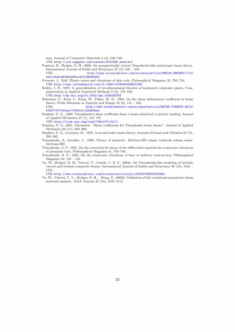
sion. Journal of Composite Materials 4 (4), 538–548.URL http://jcm.sagepub.com/content/4/4/538.abstract

Popescu, B., Hodges, D. H., 2000. On asymptotically correct Timoshenko-like anisotropic beam theory.International Journal of Solids and Structures 37 (3), 535 – 558.URL http://www.sciencedirect.com/science/article/B6VJS-3XM2SF5-7/2/

aefcc4a6cdb0debe8fe1d1f196b8e623

Prescott, J., 1942. Elastic waves and vibrations of thin rods. Philosophical Magazine 33, 703–754.URL http://www.informaworld.com/10.1080/14786444208521261

Reddy, J. N., 1987. A generalization of two-dimensional theories of laminated composite plates. Com-munications in Applied Numerical Methods 3 (3), 173–180.URL http://dx.doi.org/10.1002/cnm.1630030303

Schramm, U., Kitis, L., Kang, W., Pilkey, W. D., 1994. On the shear deformation coefficient in beamtheory. Finite Elements in Analysis and Design 16 (2), 141 – 162.URL http://www.sciencedirect.com/science/article/B6V36-47X88CD-4W/2/

b29277277d1bae17f590c51c25db3ba4

Stephen, N. G., 1980. Timoshenko’s shear coefficient from a beam subjected to gravity loading. Journalof Applied Mechanics 47 (1), 121–127.URL http://link.aip.org/link/?AMJ/47/121/1

Stephen, N. G., 2001. Discussion: “Shear coefficients for Timoshenko beam theory”. Journal of AppliedMechanics 68 (11), 959–960.

Stephen, N. G., Levinson, M., 1979. A second order beam theory. Journal of Sound and Vibration 67 (3),293–305.

Timoshenko, S., Goodier, J., 1969. Theory of elasticity. McGraw-Hill classic textbook reissue series.McGraw-Hill.

Timoshenko, S. P., 1921. On the correction for shear of the differential equation for transverse vibrationsof prismatic bars. Philosophical Magazine 41, 744–746.

Timoshenko, S. P., 1922. On the transverse vibrations of bars of uniform cross-section. PhilosophicalMagazine 43, 125 – 131.

Yu, W., Hodges, D. H., Volovoi, V., Cesnik, C. E. S., 2002a. On Timoshenko-like modeling of initiallycurved and twisted composite beams. International Journal of Solids and Structures 39 (19), 5101 –5121.URL http://www.sciencedirect.com/science/article/pii/S0020768302003992

Yu, W., Volovoi, V. V., Hodges, D. H., , Hong, X., 2002b. Validation of the variational asymptotic beamsectional analysis. AIAA Journal 40 (10), 2105–2112.

35

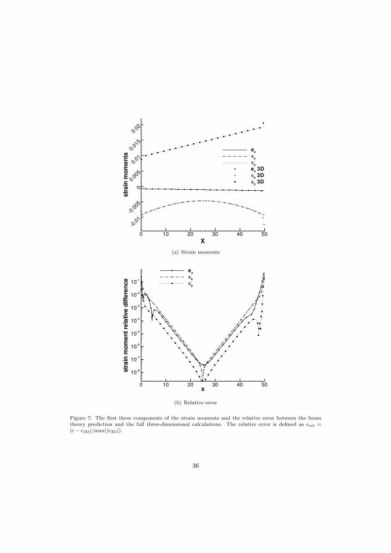
X

strain

moments

0 10 20 30 40 50

­0.0

1

­0.0

05

0

0.0

05

0.0

1

0.0

15

0.0

2

ex

κz

κy

ex3D

κz3D

κy3D

(a) Strain moments

x

strain

momentrelativedifference

0 10 20 30 40 50

10­8

10­7

10­6

10­5

10­4

10­3

10­2

10­1

ex

κz

κy

(b) Relative error

Figure 7: The first three components of the strain moments and the relative error between the beamtheory prediction and the full three-dimensional calculations. The relative error is defined as erel =|e− e3D|/max(|e3D|).

36

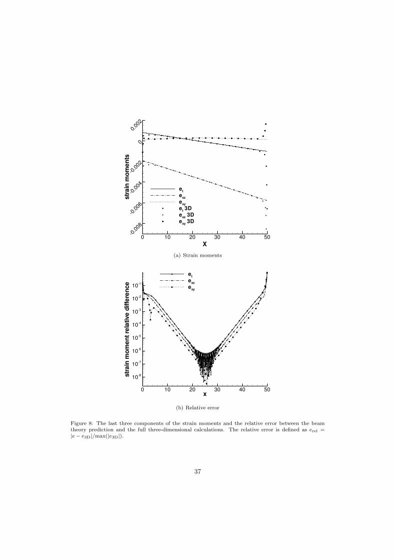
X

strain

moments

0 10 20 30 40 50­0

.008

­0.0

06

­0.0

04

­0.0

02

0

0.0

02

et

exz

exy

et3D

exz3D

exy3D

(a) Strain moments

x

strain

momentrelativedifference

0 10 20 30 40 50

10­8

10­7

10­6

10­5

10­4

10­3

10­2

10­1

et

exz

exy

(b) Relative error

Figure 8: The last three components of the strain moments and the relative error between the beamtheory prediction and the full three-dimensional calculations. The relative error is defined as erel =|e− e3D|/max(|e3D|).

37

x

relativemoments

ofthestrain

residual

0 10 20 30 40 5010

­9

10­8

10­7

10­6

10­5

10­4

10­3

10­2

10­1

100

ex

κz

exz

Figure 9: Components of the relative moments of the strain residual Lsε|3D normalized by the max-imum absolute values of the strain moment over the domain. These quantities are computed from acombination of the finite-element solution and the beam theory using Equation (48). These componentsare representative of the remaining components.

x

relativestrain

correctionerror

0 10 20 30 40 5010

­9

10­8

10­7

10­6

10­5

10­4

10­3

10­2

10­1

100

et

exz

exy

Figure 10: Components of the relative strain correction error. The strain correction error is normalizedby the maximum absolute values of the strain moment over the domain.

38

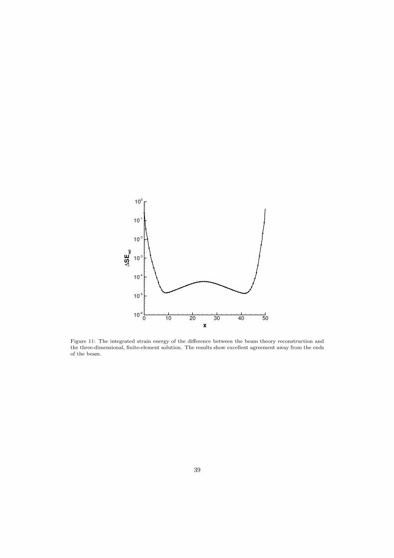
x

∆SE

rel

0 10 20 30 40 5010

­6

10­5

10­4

10­3

10­2

10­1

100

Figure 11: The integrated strain energy of the difference between the beam theory reconstruction andthe three-dimensional, finite-element solution. The results show excellent agreement away from the endsof the beam.

39

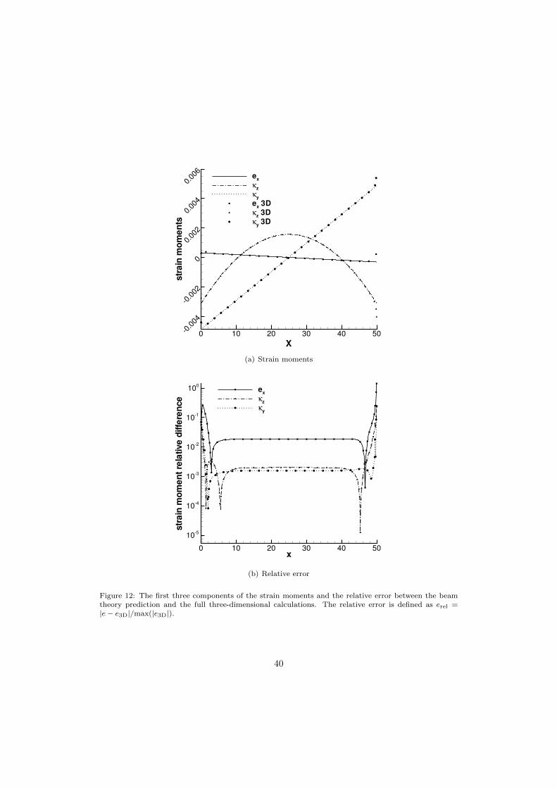
X

strain

moments

0 10 20 30 40 50­0.0

04

­0.0

02

0

0.0

02

0.0

04

0.0

06

ex

κz

κy

ex3D

κz3D

κy3D

(a) Strain moments

x

strain

momentrelativedifference

0 10 20 30 40 50

10­5

10­4

10­3

10­2

10­1

100

ex

κz

κy

(b) Relative error

Figure 12: The first three components of the strain moments and the relative error between the beamtheory prediction and the full three-dimensional calculations. The relative error is defined as erel =|e− e3D|/max(|e3D|).

40

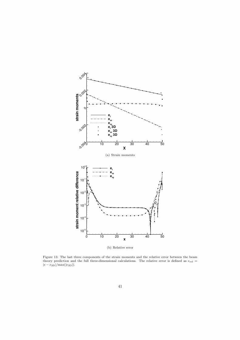
X

strain

moments

0 10 20 30 40 50

­0.0

04

­0.0

02

0

0.0

02

0.0

04

et

exz

exy

et3D

exz3D

exy3D

(a) Strain moments

x

strain

momentrelativedifference

0 10 20 30 40 50

10­5

10­4

10­3

10­2

10­1

100

et

exz

exy

(b) Relative error

Figure 13: The last three components of the strain moments and the relative error between the beamtheory prediction and the full three-dimensional calculations. The relative error is defined as erel =|e− e3D|/max(|e3D|).

41

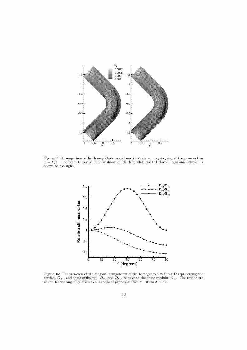
Y

Z

­1 ­0.5 0 0.5

­1.5

­1

­0.5

0

0.5

1

1.5

Y

Z

­1 ­0.5 0 0.5

­1.5

­1

­0.5

0

0.5

1

1.5

0.0017

0.0008

­0.0001

­0.001

εV

Figure 14: A comparison of the through-thickness volumetric strain εV = εx+εy +εz at the cross-sectionx = L/2. The beam theory solution is shown on the left, while the full three-dimensional solution isshown on the right.

θ [degrees]

Relativestiffnessvalue

0 15 30 45 60 75 90

0.6

0.8

1

1.2

1.4

1.6

1.8 D44/G

12

D55/G

12

D66/G

12

Figure 15: The variation of the diagonal components of the homogenized stiffness D representing thetorsion, D44, and shear stiffnesses, D55 and D66, relative to the shear modulus G12. The results areshown for the angle-ply beam over a range of ply angles from θ = 0o to θ = 90o.

42

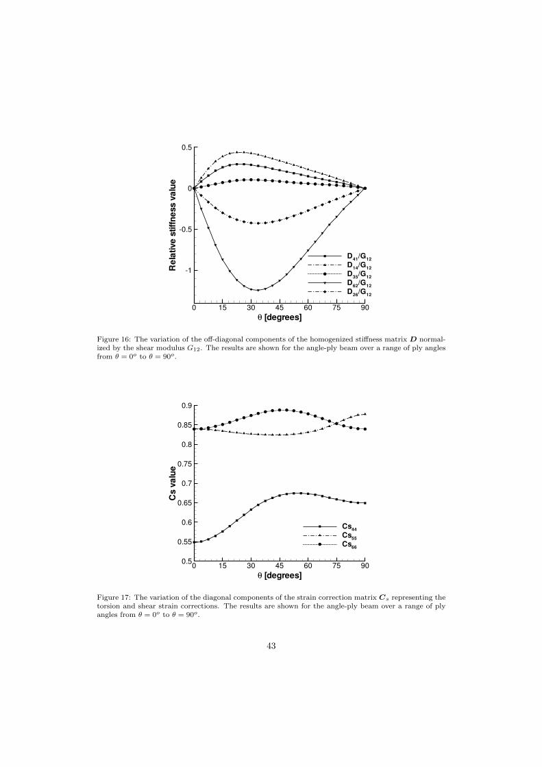
θ [degrees]

Relativestiffnessvalue

0 15 30 45 60 75 90

­1

­0.5

0

0.5

D41/G

12

D14/G

12

D35/G

12

D62/G

12

D26/G

12

Figure 16: The variation of the off-diagonal components of the homogenized stiffness matrix D normal-ized by the shear modulus G12. The results are shown for the angle-ply beam over a range of ply anglesfrom θ = 0o to θ = 90o.

θ [degrees]

Csvalue

0 15 30 45 60 75 900.5

0.55

0.6

0.65

0.7

0.75

0.8

0.85

0.9

Cs44

Cs55

Cs66

Figure 17: The variation of the diagonal components of the strain correction matrix Cs representing thetorsion and shear strain corrections. The results are shown for the angle-ply beam over a range of plyangles from θ = 0o to θ = 90o.

43

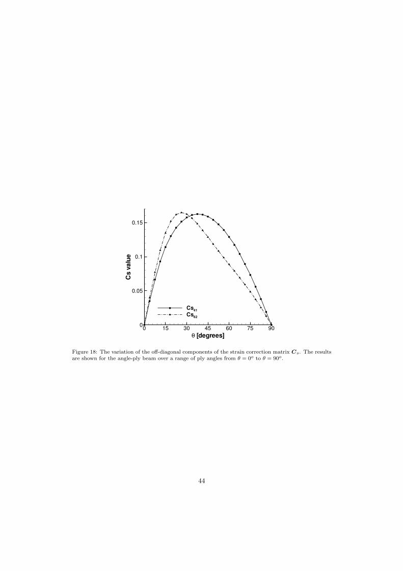
θ [degrees]

Csvalue

0 15 30 45 60 75 900

0.05

0.1

0.15

Cs41

Cs62

Figure 18: The variation of the off-diagonal components of the strain correction matrix Cs. The resultsare shown for the angle-ply beam over a range of ply angles from θ = 0o to θ = 90o.

44