Embed Size (px)
Citation preview

1
A Holistic Approach to Sensorand Analytical Method
Development
Barry M. Wise, Neal B. Gallagher,
Richard M. Ozanich,* and Jay Grate*
*Pacific Northwest National Laboratory
Richland, WA USA
United States

2
Washington State
Neal
Barry
Rich, Jay
• Concept of holistic design
• Examples• Laser Photo-acoustic Spectroscopy Sensor
• GC-Surface Acoustic Wave Sensor
Outline

3
Holistic Design Concept
• Analytical systems can not be optimized one pieceat a time
• Model the whole analytical system, from sampleenvironment to output
• Lots of parts to consider
Overall Model
SampleEnvironment
Analytical Device
(hardware)
Data Analysis(software)
Estimate

4
Sample Environment Model
• Analytes of interest
• Interferents, mean, covariance, distribution
• Specific problem interferents
• Situation specific scenarios
• Sampling error
Analytical Instrument Model
• Typically a blend of theoretical, empirical andstatistical elements
• Ideal response
• Noise model
• Non-idealities
• Sensor selection

5
Data Analysis
• Detection, concentration, classification…
• What sort of model?
• How to calibrate?
Exercising the Models
• Monte Carlo
• Can sometimes propagate theoretically
• Often interested in the distribution tails

6
Model Use
SampleEnvironment
Analytical Device
(hardware)
Data Analysis(software)
Estimate
Device configurationVariable selection
Power, signal
PLS, CLS, GLS,PLS-DA, GRAM
Potential probleminterferents
Optimizationor what if?
Example 1
• Laser Photo-acoustic Spectroscopy Sensor
• Detection of G-agents in battlefield scenario
• DARPA project lead by PNNL
• Reference:• Laser photo-acoustic chemical sensor performance
modeling, J. F. Schultz, B. D. Cannon, T. L. Myers, R.M. Ozanich, D. M. Sheen, M. S. Taubman, M. D.Wojcik, N. B. Gallagher, B. M. Wise, Proceedings
of SPIE Vol. #57
7
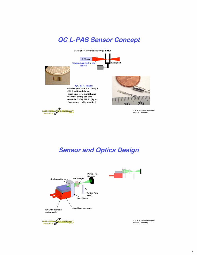
QC L-PAS Sensor Concept
QC & IC lasers:•Wavelengths from ~ 2 – 100 μm
•FM & AM modulation
•Small sizes for multiplexing
• ~10 cm-1 tuning per laser
• 600 mW CW @ 300 K, (6 μm)
•Repeatable, readily stabilized
Compact, rugged in situ
sensors
QC Laser
Tuning Fork
Laser photo-acoustic sensors (L-PAS):
U.S. DOE - Pacific Northwest
National LaboratoryDARPA MTO
Sensor and Optics Design
Lens Mount
Chalcogenide Lens
Tuning Fork
(QVR)
Pyroelectric
DetectorZnSe Window
Liquid heat exchangerTEC with diamond
heat spreader
U.S. DOE - Pacific Northwest
National LaboratoryDARPA MTO

8
QVR Voltage and Noise Sources
• P –Power in QCL mode • Varies more than total QCL power
except for single mode QCL• Measure total QCL power to 1%
relative reproducibility• Cross Section chem,
• Varies with wavelength and hencelaser line shape and laser chirp
• Chemical Concentrations-CChem• Analyte & clutter (both vary)
• Thermal Noise in QVR• Analogous to Johnson noise• Limits sensitivity in Rice expts.
• Acoustic Interference at AM frequency• AM laser power absorbed by QVR &
other surfaces• Measure to generate specs for optics
design• Variations in QCL power and coupling to
QVR create noise• Preamp gain Zgain• Acoustic coupling coefficients (A1, A2,solid )
++= seThermalNoiPAPCAZVSolid
Solid
Chem
ChemChemgainQVR ,2,1
U.S. DOE - Pacific Northwest
National LaboratoryDARPA MTO
Simulant Spectra in the Long-Wave IR
700 800 900 1000 1100 1200 1300 1400 15000.99
1
700 800 900 1000 1100 1200 1300 1400 15000
0.001
0.002
0.003
0.004
Frequency (cm-1)
Abso
rban
ce (
bas
e 10) DMMP
Atmospheric Concentration
Analytes (ppm)
CO2 475
CO 25
NO2 0.1
CH4 0.9
H2O 784
O3 0.07
N2O 0.3
U.S. DOE - Pacific Northwest
National LaboratoryDARPA MTO

9
Simulant Spectra in the Mid-Wave IR
2100 2200 2300 2400 2500 2600 2700 2800 2900 3000 31000.99
1
2100 2200 2300 2400 2500 2600 2700 2800 2900 3000 31000
0.001
0.002
0.003
0.004
Frequency (cm-1)
Abso
rban
ce (
bas
e 10) DMMP
Atmospheric Concentration
Analytes (ppm)
CO2 475
CO 25
NO2 0.1
CH4 0.9
H2O 784
O3 0.07
N2O 0.3
U.S. DOE - Pacific Northwest
National LaboratoryDARPA MTO
Analyte Concentration (mg/m3)
CO2* 634-7065
H2O 0-1163
NO2* 0.00038-250
CO* 12-46
SO2* 0.026-13
Formaldehyde* 0.0025-3.0
CH4 0.1-1.1
Toluene 0.0076-0.76
N2O 0.36-0.7
Dodecane 0.014-0.49
H2S 0.014-0.43
Benzene* 0.0064-0.24
Parathion 0-0.24
m-Xylene* 0.0044-0.22
Acetaldehyde* 0.0036-0.22
O3 0.059-0.2
DEET 0-0.16
Propionaldehyde* 0.0024-0.14
HNO3 0-0.065
Acrolein* 0.0023-0.06
Butadiene* 0.0022-0.038
Carbonyl Sulfide* 0.0025-0.032
NH3 0.00002-0.0035
HCN 0-0.0011
Ethylene Glycol 0-0.00026
* Diesel constituent
Initial Design Atmosphere• “Standard” constituents
vary independently
between mean values of
EPA rural and urban
atmospheres
• Only species with IR
absorptions are listed at
right
• Single-component
interferents vary from 0 to
max value
• Diesel exhaust
constituents co-vary
(R2=0.8) from 0 to max
values (close proximity to
running diesel engine)
TA Blake, KM Probasco , “Chemical Emission
Scenarios and Detection Limits for Active
Infrared Remote Sensing”, PNNL Report
13382 (2000).
U.S. DOE - Pacific Northwest
National LaboratoryDARPA MTO

10
Pre- concentrator
Core containing solid adsorbent
Resistive Heating Wires
U.S. DOE - Pacific Northwest
National LaboratoryDARPA MTO
Initial Design Atmosphere With Pre-concentration
Analyte Concentration (mg/m3)
CO2* 634-7065
H2O5 0-5815
NO2* 0.00038-250
CO* 12-46
SO2* 0.026-13
Formaldehyde* 0.0025-3.0
CH4 0.1-1.1
Toluene10 0.076-7.6
N2O 0.36-0.7
Dodecane10 0.14-4.9
H2S5 0.07-2.15
Benzene*10 0.064-2.4
Parathion10 0-2.4
m-Xylene*10 0.044-2.2
Acetaldehyde*5 0.018-1.1
O3 0.059-0.2
DEET10 0-1.6
Propionaldehyde*5 0.012-0.7
HNO310 0-0.65
Acrolein*5 0.0115-0.3
Butadiene*5 0.011-0.19
Carbonyl Sulfide* 0.0025-0.032
NH310 0.0002-0.035
HCN 0-0.0011
Ethylene Glycol10 0-0.0026
Concentrations shown assume pre-concentration,
resulting in 10-fold concentration of agents and
the following concentration factors for
interferents:
5 = 5-Fold Concentration Factor10 = 10-Fold Concentration Factor
* = Diesel Exhaust Constituent
U.S. DOE - Pacific Northwest
National LaboratoryDARPA MTO

11
Fabry-Perot QCL Line-shapes
Near threshold, CWoperation:•Single mode•Width < 3 cm-1
Initial design choice
Well above threshold, 100%current modulation:
•Multiple modes
•Width ~10 cm-1
•Relative mode power stability?
Well above threshold, CW:
•Multiple modes
•Width ~ 50 cm-1 wide (!)
•Relative mode power stability?
J. S. Yu, A. Evans, J. David, L. Doris, S.Slivken, and M. Razeghi, IEEE PHOTONICSTECHNOLOGY LETTERS, VOL. 16, NO. 3, pp747-9, MARCH 2004
M. Garcia a, E. Normand b, C.R.
Stanley a, C.N. Ironside, C.D. Farmer,G. Duxbury, and N. Langford, OpticsComm 2003
Lineshape from 12 A, 9 ns
pulsed QC laser
Lineshape from CW, 25 C QCL
producing ~80 mWLineshape from Maxion QCL, CW
cryogenic operation, 56 mW
1130 1150 1170 11900
0.1
0.2 FP 10.99 mW
FP 55.95 mW
U.S. DOE - Pacific Northwest
National LaboratoryDARPA MTO
QVR Voltage and Noise Sources
• P –Power in QCL mode • Varies more than total QCL power
except for single mode QCL• Measure total QCL power to 1%
relative reproducibility• Cross Section chem,
• Varies with wavelength and hencelaser line shape and laser chirp
• Chemical Concentrations-CChem• Analyte & clutter (both vary)
• Thermal Noise in QVR• Analogous to Johnson noise• Limits sensitivity in Rice expts.
• Acoustic Interference at AM frequency• AM laser power absorbed by QVR &
other surfaces• Measure to generate specs for optics
design• Variations in QCL power and coupling to
QVR create noise• Preamp gain Zgain• Acoustic coupling coefficients (A1, A2,solid )
++= seThermalNoiPAPCAZVSolid
Solid
Chem
ChemChemgainQVR ,2,1
U.S. DOE - Pacific Northwest
National LaboratoryDARPA MTO

12
Noise Model for QC L-PAS Initial Design
• Proportional noise due to QCL powervariations
• 1% relative noise using power measurement
• Additive thermal noise• RQVR
• Neglect background from solids• Assumes good optics so laser beam clears QVR• Weak coupling of distant acoustic sources to
QVR
• Neglect variations in laser chirp
)(4.1
1.090
300410
4
rmsV
Hzk
KkM
fR
kTZNoiseThermal
QVR
gain
μ=
°=
=
++= seThermalNoiPAPCAZVSolid
Solid
Chem
ChemChemgainQVR ,2,1
U.S. DOE - Pacific Northwest
National LaboratoryDARPA MTO
Laser Line Selection Using Partial Least Squares Discriminant
Analysis (PLS-DA)
1. Generate synthetic data with and without agent:- Use 500 null spectra (clutter plus interferents plus noise) and 125 positive
spectra (clutter plus interferents plus noise plus signal) for each G-agent,with concentrations ranging from 0.02-0.1 mg/m3.
- Repeat null spectra and G-agent spectra creation 20 times to check forconsistency of regression vector produced from PLS-DA (below)
2. Calculate a regression vector b which is the PLS best fit solution to theequation
X b = y,
where X is a matrix of the synthetic spectra, and y is a vector that classifieseach spectrum as positive or null.
3. Plot b and select laser lines that contain the most information.
U.S. DOE - Pacific Northwest
National LaboratoryDARPA MTO

13
• Select laser lines based on regression coefficients
from regression vector
• Positive peaks correspond to agent features
• Negative peaks account for overlapping
interferences
• Select lines with large (+/-) coefficients
• Choose lines >20 cm-1 apart and where regression
coefficients don’t change rapidly to allow for
broader laser lines and drift
• Choose lines on separate features to provide unique
information
Laser Line Selection
U.S. DOE - Pacific Northwest
National LaboratoryDARPA MTO
Calculation of ROC Curves
1 million spectra with and without
agent were generated.
The red curve represents the values of
y calculated from distribution of the
samples not containing agent. The
blue curve corresponds to values of y
calculated from the distribution of
samples containing agent at 0.044
mg/m3.
The vertical green line is placed so the
false negative rate (the fractional area
under the blue curve to the left of the
green line) is at the chosen PD.
The false positive rate can then be
calculated (the fractional area under
the red curve to the right of the green
line), in this example it is 6.3 X 10⁻³.
The process is then repeated at
different agent concentrations.
To generate one point on a ROC curve, a specific agent concentration and defined false negative rate are chosen.
For this example, a 5% false negative rate was chosen (represented by the 95% PD – vertical green line).
Null distribution Distribution of Cyclosarin at0.044 mg/m3
False Positive Rate Area = 0.0063
False Negative RateArea = 0.05
95% PDLine
Position on PLS-DA Regression Vector
U.S. DOE - Pacific Northwest
National LaboratoryDARPA MTO

14
ROC Curves with and without Preconcentrator
10-6
10-5
10-4
10-3
10-2
10-1
0
0.1
0.2
0.3
0.4
0.5
Co
nce
ntr
atio
n (
mg
/m3
)
False Positive Rate (per sample)
Tabun (GA) ROC Curves, 95% PD
Initial Design (Preconcentration)
No Preconcentration
10-6
10-5
10-4
10-3
10-2
10-1
0
0.1
0.2
0.3
10-6
10-5
10-4
10-3
10-2
10-1
0
0.1
0.2
0.3
0.4
0.5
Co
nce
ntr
atio
n (
mg
/m3
)
False Positive Rate (per sample)
Tabun (GA) ROC Curves, 95% PD
Initial Design (Preconcentration)
No Preconcentration
10-6
10-5
10-4
10-3
10-2
10-1
0
0.1
0.2
0.3
0.4
0.5
Co
nce
ntr
atio
n (
mg
/m3
)
False Positive Rate (per sample)
Sarin (GB) ROC Curves, 95% PD
Initial Design (Preconcentration)
No Preconcentration
10-6
10-5
10-4
10-3
10-2
10-1
0
0.1
0.2
0.3
10-6
10-5
10-4
10-3
10-2
10-1
0
0.1
0.2
0.3
0.4
0.5
Co
nce
ntr
atio
n (
mg
/m3
)
False Positive Rate (per sample)
Sarin (GB) ROC Curves, 95% PD
Initial Design (Preconcentration)
No Preconcentration
10-6
10-5
10-4
10-3
10-2
10-1
0
0.1
0.2
0.3
0.4
0.5
Co
nce
ntr
atio
n (
mg
/m3
)
False Positive Rate (per sample)
Soman (GD) ROC Curves, 95% PD
Initial Design (Preconcentration)
No Preconcentration
10-6
10-5
10-4
10-3
10-2
10-1
0
0.1
0.2
0.3
10-6
10-5
10-4
10-3
10-2
10-1
0
0.1
0.2
0.3
0.4
0.5
Co
nce
ntr
atio
n (
mg
/m3
)
False Positive Rate (per sample)
Soman (GD) ROC Curves, 95% PD
Initial Design (Preconcentration)
No Preconcentration
10-6
10-5
10-4
10-3
10-2
10-1
0
0.1
0.2
0.3
0.4
0.5
Co
nce
ntr
atio
n (
mg
/m3
)False Positive Rate (per sample)
Cyclosarin (GF) ROC Curves, 95% PD
Initial Design (Preconcentration)
No Preconcentration
10-6
10-5
10-4
10-3
10-2
10-1
0
0.1
0.2
0.3
10-6
10-5
10-4
10-3
10-2
10-1
0
0.1
0.2
0.3
0.4
0.5
Co
nce
ntr
atio
n (
mg
/m3
)False Positive Rate (per sample)
Cyclosarin (GF) ROC Curves, 95% PD
Initial Design (Preconcentration)
No Preconcentration
U.S. DOE - Pacific Northwest
National LaboratoryDARPA MTO
ROC Curves with Estimated and Low Noise (33% of est.)
10-6
10-5
10-4
10-3
10-2
10-1
0.02
0.04
0.06
0.08
0.1
Conce
ntr
atio
n (
mg/m
3)
False Positive Rate (per sample)
Tabun (GA) ROC Curves, 95% PD
Initial Design (Preconcentration)
Low Noise
10-6
10-5
10-4
10-3
10-2
10-1
0.02
0.04
10-6
10-5
10-4
10-3
10-2
10-1
0.02
0.04
0.06
0.08
0.1
Conce
ntr
atio
n (
mg/m
3)
False Positive Rate (per sample)
Tabun (GA) ROC Curves, 95% PD
Initial Design
Low Noise
10-6
10-5
10-4
10-3
10-2
10-1
0.02
0.04
0.06
0.08
0.1
Conce
ntr
atio
n (
mg/m
3)
False Positive Rate (per sample)
Sarin (GB) ROC Curves, 95% PD
Initial Design (Preconcentration)
Low Noise
10-6
10-5
10-4
10-3
10-2
10-1
0.02
0.04
10-6
10-5
10-4
10-3
10-2
10-1
0.02
0.04
0.06
0.08
0.1
Conce
ntr
atio
n (
mg/m
3)
False Positive Rate (per sample)
Sarin (GB) ROC Curves, 95% PD
Initial Design
Low Noise
10-6
10-5
10-4
10-3
10-2
10-1
0.02
0.04
0.06
0.08
0.1
Conce
ntr
atio
n (
mg/m
3)
False Positive Rate (per sample)
Soman (GD) ROC Curves, 95% PD
Initial Design (Preconcentration)
Low Noise
10-6
10-5
10-4
10-3
10-2
10-1
0.02
0.04
10-6
10-5
10-4
10-3
10-2
10-1
0.02
0.04
0.06
0.08
0.1
Conce
ntr
atio
n (
mg/m
3)
False Positive Rate (per sample)
Soman (GD) ROC Curves, 95% PD
Initial Design
Low Noise
10-6
10-5
10-4
10-3
10-2
10-1
0.02
0.04
0.06
0.08
0.1
Conce
ntr
atio
n (
mg/m
3)
False Positive Rate (per sample)
Cyclosarin (GF) ROC Curves, 95% PD
Initial Design (Preconcentration)
Low Noise
10-6
10-5
10-4
10-3
10-2
10-1
0.02
0.04
10-6
10-5
10-4
10-3
10-2
10-1
0.02
0.04
0.06
0.08
0.1
Conce
ntr
atio
n (
mg/m
3)
False Positive Rate (per sample)
Cyclosarin (GF) ROC Curves, 95% PD
Initial Design
Low Noise
U.S. DOE - Pacific Northwest
National LaboratoryDARPA MTO
15
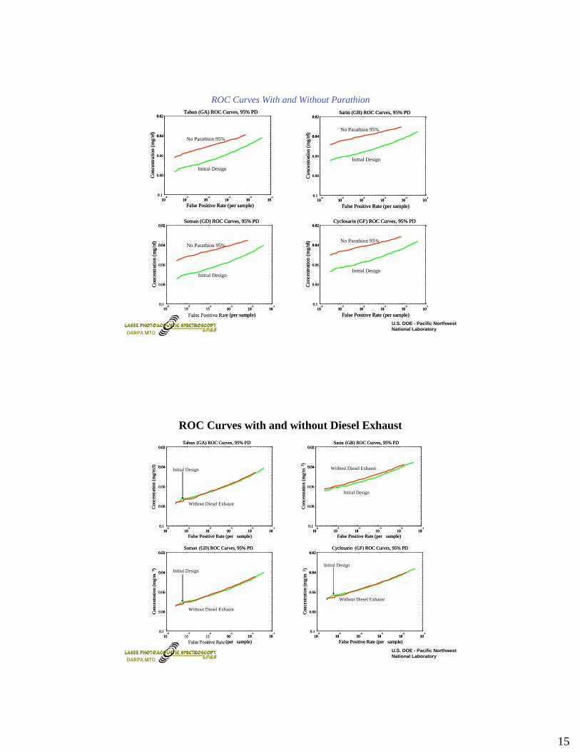
ROC Curves With and Without Parathion
10-6
10-5
10-4
10-3
10-2
10-1
0.02
0.04
0.06
0.08
0.1
Conce
ntr
atio
n (
mg/m
3 )
False Positive Rate (per sample)
Tabun (GA) ROC Curves, 95% PD
Initial Design (Preconcentration)
No Parathion 95%
10-6
10-5
10-4
10-3
10-2
10-1
0.02
0.04
10-6
10-5
10-4
10-3
10-2
10-1
0.02
0.04
0.06
0.08
0.1
Conce
ntr
atio
n (
mg/m
3 )
False Positive Rate (per sample)
Tabun (GA) ROC Curves, 95% PD
Initial Design
No Parathion 95%
10-6
10-5
10-4
10-3
10-2
10-1
0.02
0.04
0.06
0.08
0.1
Conce
ntr
atio
n (
mg/m
3)
False Positive Rate (per sample)
Sarin (GB) ROC Curves, 95% PD
Initial Design (Preconcentration)
No Parathion 95%
10-6
10-5
10-4
10-3
10-2
10-1
0.02
0.04
10-6
10-5
10-4
10-3
10-2
10-1
0.02
0.04
0.06
0.08
0.1
Conce
ntr
atio
n (
mg/m
3)
False Positive Rate (per sample)
Sarin (GB) ROC Curves, 95% PD
Initial Design
No Parathion 95%
10-6
10-5
10-4
10-3
10-2
10-1
0.02
0.04
0.06
0.08
0.1
Conce
ntr
atio
n (
mg/m
3)
False Positive Rate (per sample)
Soman (GD) ROC Curves, 95% PD
Initial Design (Preconcentration)
No Parathion 95%
10-6
10-5
10-4
10-3
10-2
10-1
0.02
0.04
10-6
10-5
10-4
10-3
10-2
10-1
0.02
0.04
0.06
0.08
0.1
Conce
ntr
atio
n (
mg/m
3)
False Positive Rate (per sample)
Soman (GD) ROC Curves, 95% PD
Initial Design
No Parathion 95%
10-6
10-5
10-4
10-3
10-2
10-1
0.02
0.04
0.06
0.08
0.1 C
once
ntr
atio
n (
mg/m
3)
False Positive Rate (per sample)
Cyclosarin (GF) ROC Curves, 95% PD
Initial Design (Preconcentration)
No Parathion 95%
10-6
10-5
10-4
10-3
10-2
10-1
0.02
0.04
10-6
10-5
10-4
10-3
10-2
10-1
0.02
0.04
0.06
0.08
0.1 C
once
ntr
atio
n (
mg/m
3)
False Positive Rate (per sample)
Cyclosarin (GF) ROC Curves, 95% PD
Initial Design
No Parathion 95%
U.S. DOE - Pacific Northwest
National LaboratoryDARPA MTO
ROC Curves with and without Diesel Exhaust
10-6
10-5
10-4
10-3
10-2
10-1
0.02
0.04
0.06
0.08
0.1
Conce
ntr
atio
n (
mg/m
3)
False Positive Rate (per sample)
Tabun (GA) ROC Curves, 95% PD
Initial Design (Preconcentration)
Without Diesel Exhaust
10-6
10-5
10-4
10-3
10-2
10-1
0.02
0.04
10-6
10-5
10-4
10-3
10-2
10-1
0.02
0.04
0.06
0.08
0.1
Conce
ntr
atio
n (
mg/m
3)
False Positive Rate (per sample)
Tabun (GA) ROC Curves, 95% PD
Initial Design
Without Diesel Exhaust
10-6
10-5
10-4
10-3
10-2
10-1
0.02
0.04
0.06
0.08
0.1
Conce
ntr
atio
n (
mg/m
3)
False Positive Rate (per sample)
Sarin (GB) ROC Curves, 95% PD
Initial Design (Preconcentration)
Without Diesel Exhaust
10-6
10-5
10-4
10-3
10-2
10-1
0.02
0.04
10-6
10-5
10-4
10-3
10-2
10-1
0.02
0.04
0.06
0.08
0.1
Conce
ntr
atio
n (
mg/m
3)
False Positive Rate (per sample)
Sarin (GB) ROC Curves, 95% PD
Initial Design
Without Diesel Exhaust
10-6
10-5
10-4
10-3
10-2
10-1
0.02
0.04
0.06
0.08
0.1
Conce
ntr
atio
n (
mg/m
3)
False Positive Rate (per sample)
Soman (GD) ROC Curves, 95% PD
Initial Design (Preconcentration)
Without Diesel Exhaust
10-6
10-5
10-4
10-3
10-2
10-1
0.02
0.04
10-6
10-5
10-4
10-3
10-2
10-1
0.02
0.04
0.06
0.08
0.1
Conce
ntr
atio
n (
mg/m
3)
False Positive Rate (per sample)
Soman (GD) ROC Curves, 95% PD
Initial Design
Without Diesel Exhaust
10-6
10-5
10-4
10-3
10-2
10-1
0.02
0.04
0.06
0.08
0.1
Conce
ntr
atio
n (
mg/m
3)
False Positive Rate (per sample)
Cyclosarin (GF) ROC Curves, 95% PD
Initial Design (Preconcentration)
Without Diesel Exhaust
10-6
10-5
10-4
10-3
10-2
10-1
0.02
0.04
10-6
10-5
10-4
10-3
10-2
10-1
0.02
0.04
0.06
0.08
0.1
Conce
ntr
atio
n (
mg/m
3)
False Positive Rate (per sample)
Cyclosarin (GF) ROC Curves, 95% PD
Initial Design
Without Diesel Exhaust
U.S. DOE - Pacific Northwest
National LaboratoryDARPA MTO

16
ROC Curves for G-Agent Categories: GA & Non-GA
10-6
10-5
10-4
10-3
10-2
10-1
0.02
0.04
0.06
0.08
0.1
Conce
ntr
atio
n (
mg/m
3)
False Positive Rate (per sample)
Tabun (GA) ROC Curves, 95% PD
Initial Design (Preconcentration)
Tabun Specific Model
10-6
10-5
10-4
10-3
10-2
10-1
0.02
0.04
10-6
10-5
10-4
10-3
10-2
10-1
0.02
0.04
0.06
0.08
0.1
Conce
ntr
atio
n (
mg/m
3)
False Positive Rate (per sample)
Tabun (GA) ROC Curves, 95% PD
Initial Design
Tabun Specific Model
10-6
10-5
10-4
10-3
10-2
10-1
0.02
0.04
0.06
0.08
0.1
Conce
ntr
atio
n (
mg/m
3)
False Positive Rate (per sample)
Sarin (GB) ROC Curves, 95% PD
Initial Design (Preconcentration)
G-Agent Model (No Tabun)
10-6
10-5
10-4
10-3
10-2
10-1
0.02
0.04
10-6
10-5
10-4
10-3
10-2
10-1
0.02
0.04
0.06
0.08
0.1
Conce
ntr
atio
n (
mg/m
3)
False Positive Rate (per sample)
Sarin (GB) ROC Curves, 95% PD
Initial Design
Non-GA Model (No Tabun)
10-6
10-5
10-4
10-3
10-2
10-1
0.02
0.04
0.06
0.08
0.1
Conce
ntr
atio
n (
mg/m
3)
False Positive Rate (per sample)
Soman (GD) ROC Curves, 95% PD
Initial Design (Preconcentration)
G-Agent Model (No Tabun)
10-6
10-5
10-4
10-3
10-2
10-1
0.02
0.04
10-6
10-5
10-4
10-3
10-2
10-1
0.02
0.04
0.06
0.08
0.1
Conce
ntr
atio
n (
mg/m
3)
False Positive Rate (per sample)
Soman (GD) ROC Curves, 95% PD
Initial Design
Non-GA Model (No Tabun)
10-6
10-5
10-4
10-3
10-2
10-1
0.02
0.04
0.06
0.08
0.1 C
once
ntr
atio
n (
mg/m
3)
False Positive Rate (per sample)
Cyclosarin (GF) ROC Curves, 95% PD
Initial Design (Preconcentration)
G-Agent Model (No Tabun)
10-6
10-5
10-4
10-3
10-2
10-1
0.02
0.04
10-6
10-5
10-4
10-3
10-2
10-1
0.02
0.04
0.06
0.08
0.1 C
once
ntr
atio
n (
mg/m
3)
False Positive Rate (per sample)
Cyclosarin (GF) ROC Curves, 95% PD
Initial Design
Non-GA Model (No Tabun)
U.S. DOE - Pacific Northwest
National LaboratoryDARPA MTO
ROC Curves for Agent Specific Models vs. Initial Design
10-6
10-5
10-4
10-3
10-2
10-1
0.02
0.04
10-6
10-5
10-4
10-3
10-2
10-1
0.02
0.04
0.06
0.08
0.1
Conce
ntr
atio
n (
mg/m
3)
False Positive Rate (per sample)
Tabun (GA) ROC Curves, 95% PD
Initial Design
Tabun Only Model
10-6
10-5
10-4
10-3
10-2
10-1
0.02
0.04
0.06
0.08
0.1
Conce
ntr
atio
n (
mg/m
3)
False Positive Rate (per sample)
Sarin (GB) ROC Curves, 95% PD
Initial Design
Sarin Only Model
10-6
10-5
10-4
10-3
10-2
10-1
0.02
0.04
10-6
10-5
10-4
10-3
10-2
10-1
0.02
0.04
0.06
0.08
0.1
Conce
ntr
atio
n (
mg/m
3)
False Positive Rate (per sample)
Soman (GD) ROC Curves, 95% PD
Initial Design
Soman Only Model
10-6
10-5
10-4
10-3
10-2
10-1
0.02
0.04
10-6
10-5
10-4
10-3
10-2
10-1
0.02
0.04
0.06
0.08
0.1
Conce
ntr
atio
n (
mg/m
3)
False Positive Rate (per sample)
Cyclosarin (GF) ROC Curves, 95% PD
Initial Design
Cyclosarin Only Model
U.S. DOE - Pacific Northwest
National LaboratoryDARPA MTO

17
ROC Curves for G-Agents with 10, 15 & 20 laser lines
10-6
10-5
10-4
10-3
10-2
10-1
0.02
0.04
10-6
10-5
10-4
10-3
10-2
10-1
0.02
0.04
0.06
0.08
0.1
Co
nce
ntr
atio
n (
mg
/m3
)
False Positive Rate (per sample)
Tabun (GA) ROC Curves, 95% PD
Initial Design (Preconcentration)
With 10 Lines
20 Lines
15 Lines
10-6
10-5
10-4
10-3
10-2
10-1
0.02
0.04
10-6
10-5
10-4
10-3
10-2
10-1
0.02
0.04
0.06
0.08
0.1
Co
nce
ntr
atio
n (
mg
/m3
)
False Positive Rate (per sample)
Sarin (GB) ROC Curves, 95% PD
Initial Design (Preconcentration)
With 10 Lines
20 Lines
15 Lines
10-6
10-5
10-4
10-3
10-2
10-1
0.02
0.04
10-6
10-5
10-4
10-3
10-2
10-1
0.02
0.04
0.06
0.08
0.1
Co
nce
ntr
atio
n (
mg
/m3
)
False Positive Rate (per sample)
Soman (GD) ROC Curves, 95% PD
Initial Design (Preconcentration)
With 10 Lines
20 Lines
15 Lines
10-6
10-5
10-4
10-3
10-2
10-1
0.02
0.04
10-6
10-5
10-4
10-3
10-2
10-1
0.02
0.04
0.06
0.08
0.1
Co
nce
ntr
atio
n (
mg
/m3
)
False Positive Rate (per sample)
Cyclosarin (GF) ROC Curves, 95% PD
Initial Design (Preconcentration)
With 10 Lines
20 Lines
15 Lines
U.S. DOE - Pacific Northwest
National LaboratoryDARPA MTO
QC L-PAS Performance is Weakly Dependent on PDROC Curves for G-Agents: 10-Line GA and Non-GA Models: 90, 95, 99% PD
10-6
10-5
10-4
10-3
10-2
10-1
0
0.02
0.04
0.06
0.08
0.1
Conce
ntr
atio
n (
mg/m
3)
False Positive Rate (per sample)
ROC for Tabun (GA), Optimized 10 Line, GA Only Model
90% PD95% PD99% PD
10-6
10-5
10-4
10-3
10-2
10-1
0
0.02
10-6
10-5
10-4
10-3
10-2
10-1
0
0.02
0.04
0.06
0.08
0.1
False Positive Rate (per sample)
ROC for Tabun (GA), Optimized 10 Line, GA Only Model
90% PD95% PD99% PD
10-6
10-5
10-4
10-3
10-2
10-1
0
0.02
0.04
0.06
0.08
0.1
False Positive Rate (per sample)
ROC for Sarin (GB), Optimized 10 Line, Non-GA Model
90% PD95% PD99% PD
10-6
10-5
10-4
10-3
10-2
10-1
0
0.02
10-6
10-5
10-4
10-3
10-2
10-1
0
0.02
0.04
0.06
0.08
0.1
False Positive Rate (per sample)
90% PD95% PD99% PD
Conce
ntr
atio
n (
mg/m
3)
10-6
10-5
10-4
10-3
10-2
10-1
0
0.02
0.04
0.06
0.08
0.1
False Positive Rate (per sample)
ROC for Cyclosarin (GF), Optimized 10 Line, Non-GA Model
90% PD95% PD99% PD
10-6
10-5
10-4
10-3
10-2
10-1
0
0.02
10-6
10-5
10-4
10-3
10-2
10-1
0
0.02
0.04
0.06
0.08
0.1
90% PD95% PD99% PD
Conce
ntr
atio
n (
mg/m
3)
10-6
10-5
10-4
10-3
10-2
10-1
0
0.02
0.04
0.06
0.08
0.1
False Positive Rate (per sample)
ROC for Soman (GD), Optimized 10 Line, Non-GA Model
90% PD95% PD99% PD
10-6
10-5
10-4
10-3
10-2
10-1
0
0.02
10-6
10-5
10-4
10-3
10-2
10-1
0
0.02
0.04
0.06
0.08
0.1
False Positive Rate (per sample)
90% PD95% PD99% PD
Conce
ntr
atio
n (
mg/m
3)
U.S. DOE - Pacific Northwest
National LaboratoryDARPA MTO

18
Modeling QCL Line-shapes
FP-QCL Output.
Modeled Compared to Measured.
Normalized to 1 mW.
Measured FP-QCL Output
at Different Powers
DFB-QCL Output.
Modeled Curves Generated from
Measured Output.
1100 1120 1140 1160 1180 1200
0
0.1
0.2
0.3
0.4
0.5
Frequency (cm -1)
Pow
er (
mW
)
1100 1120 1140 1160 1180 1200
0
0.1
0.2
0.3
0.4
0.5
Frequency (cm -1)
Pow
er (
mW
)
15.83 mW
9.03 mW
4.55 mW
0.05 mW
-30 -20 -10 0 10 20 300
0.01
0.02
0.03
0.04
Frequency (cm -1)
Pow
er (
mW
)
measured 15.83 mW
measured 9.03 mW
measured 4.55 mW
measured 0.5 mW
modeled
width=20 cm -1
modeled
width=15 cm -1
modeled
width=2 cm -1
modeled
width=28 cm -1
-30 -20 -10 0 10 20 300
0.01
0.02
0.03
0.04
Frequency (cm -1)
Pow
er (
mW
)
measured 15.83 mW
measured 9.03 mW
measured 4.55 mW
measured 0.5 mW
modeled
width=20 cm -1
modeled
width=15 cm -1
modeled
width=2 cm -1
modeled
width=28 cm -1
• Laser line width and shape effect the LPAS signal• Modeling the laser line obviates expense of laser construction and testing• Line width and shape can be explored using LPAS virtual sensor to guide:
• Line selection• Laser design criteria
-2 -1.5 -1 -0.5 0 0.5 1 1.5 20
0.05
0.1
0.15
0.2
0.25
Frequency (cm -1)
Lin
e P
ow
er (
mW
)
measured M62A224
width = 0.4 cm -1
width = 1 cm -1
width = 2 cm -1
-2 -1.5 -1 -0.5 0 0.5 1 1.5 20
0.05
0.1
0.15
0.2
0.25
Frequency (cm -1)
Lin
e P
ow
er (
mW
)
measured M62A224
width = 0.4 cm -1
width = 1 cm -1
width = 2 cm -1
U.S. DOE - Pacific Northwest
National LaboratoryDARPA MTO
QC L-PAS Performance Weakly Dependent on Laser Line WidthROC Curves for Cyclosarin: FP vs. DFB Line Shape
10-6
10-5
10-4
10-3
10-2
10-1
0
0.01
0.02
0.03
0.04
False Positive Rate (per cycle)
Conce
ntr
atio
n (
mg/m
3)
ROC Curves for Cyclosarin (GF): Effect of DFB Laser Line Width
width (cm -1)
1
5
15
20
10-6
10-5
10-4
10-3
10-2
10-1
0
0.01
0.02
0.03
0.04
False Positive Rate (per cycle)
Conce
ntr
atio
n (
mg/m
3)
ROC Curves for Cyclosarin (GF): Effect of DFB Laser Line Width
width (cm -1)
1
5
15
20
10-6
10-5
10-4
10-3
10-2
10-1
0
0.01
0.02
0.03
0.04
0.05
0.06
False Positive Rate (per cycle)
Conce
ntr
atio
n (
mg/m
3)
ROC Curves for Cyclosarin (GF): Effect of FP Laser Line Width
width (cm -1)5
3040
15
10-6
10-5
10-4
10-3
10-2
10-1
0
0.01
0.02
0.03
0.04
0.05
0.06
False Positive Rate (per cycle)
Conce
ntr
atio
n (
mg/m
3)
ROC Curves for Cyclosarin (GF): Effect of FP Laser Line Width
width (cm -1)5
3040
15
-10 -5 0 5 100
0.01
0.02
0.03
0.04
0.05
Frequency (cm-1)
Lin
e P
ow
er (
mW
)
width=1 cm-1
width=15 cm -1
width=5 cm -1
width=20 cm -1
-10 -5 0 5 100
0.01
0.02
0.03
0.04
0.05
Frequency (cm-1)
Lin
e P
ow
er (
mW
)
width=1 cm-1
width=15 cm -1
width=5 cm -1
width=20 cm -1
-30 -20 -10 0 10 20 300
0.01
0.02
0.03
0.04
Frequency (cm -1)
Pow
er (
mW
)
width=30 cm -1
width=15 cm -1
width=5 cm -1
width=40 cm -1
-30 -20 -10 0 10 20 300
0.01
0.02
0.03
0.04
Frequency (cm -1)
Pow
er (
mW
)
width=30 cm -1
width=15 cm -1
width=5 cm -1
width=40 cm -1
U.S. DOE - Pacific Northwest
National LaboratoryDARPA MTO

19
Model Atmosphere Analyte *Concentration (mg/m3)Water 0 - 2967Carbon dioxide 661 - 860Carbon monoxide 2.3 - 11.5Methane 1.0 - 1.2
Nitric oxide 0.25 - 2.5Nitrous oxide 0.53 - 0.65Sulfur dioxide 0.71 - 0.87Ozone 0.2 - 0.99Ethane 0.00074 - 0.62Propane 0.00073 - 0.4Ethene 0.00081 - 0.19Peroxyacetylnitrate 0.31 - 0.38n-Butane 0.000048 - 0.23Isopentane 0.0059 - 0.27Methanol 0.047 - 0.058Formaldehyde 0.0012 - 0.093
Nitric acid 0.065 - 0.13Toluene 0.0011 - 0.27Styrene 0.021 - 0.094n-Pentane 0.0021 - 0.2Methyl chloride 0.001 - 0.13Acetone 0.0048 - 0.13Isobutane 0.00072 - 0.11Methyl chloroform 0.001 - 0.25Acetylene 0.00075 - 0.047Formic acid 0.034 - 0.042Propene 0.00017 - 0.068Isoprene 0.00056 - 0.084
Hexane 0 - 0.11Dinitrogen pentoxide 0.06 - 0.073Perchloroethylene 0.0002 - 0.19Benzene 0.0029 - 0.084Isobutene 0.0069 - 0.042Ammonia 0.0063 - 0.0077…..
Concentrations for 3 typical scenarios: remote,
rural, and urban*
Over 70 analytes with significant contribution
to IR absorbance included in the model of
ambient atmosphere (partial list shown at right)
Additional analytes included in battlefield
scenario(s) and many analytes shown here will
have different concentration ranges
Model accounts for correlation in the analyte’s
concentrations (e.g. diesel exhaust components).
Information Sources.
a Finlayson -Pitts, BJ, and Pitts, JN. Chemistry of the Upper and Lower Atmosphere,
Academic Press, San Francisco. 2000. b Hobbs, PV. Introduction to Atmospheric Chemistry , Cambridge University Press,
Cambridge, UK, 2000. c Jacob, DJ. Introduction to Atmospheric Chemistry , Princeton University Press,
Princeton, New Jersey, 1999. d Seinfeld, JH, and Pandis, SN. Atmospheric Chemistry and Physics: From Air Pollution
to Climate Change , John Wiley and Sons, New York, 1998. eCalifornia Air R esources Board, Annual Toxics Summaries,
http://www.arb.ca.gov/adam/toxics/statesubstance.html
U.S. DOE - Pacific Northwest
National LaboratoryDARPA MTO
“Real World” Modeling: IR Water Continuum
1000 1500 2000 2500 300010
-8
10-7
10-6
10-5
10-4
10-3
DMMP (0.051 mg/m 3)
Continuum Absorbance
Frequency (cm -1)
Abso
rban
ce (
bas
e 10)
Increasing Temperature
Pressure = 0.5 atm
Temperature = 313 to 333 K
H2O = 1.5% volume
CO2 = 365 ppmv
1000 1500 2000 2500 300010
-8
10-7
10-6
10-5
10-4
10-3
DMMP (0.051 mg/m 3)
Continuum Absorbance
Frequency (cm -1)
Abso
rban
ce (
bas
e 10)
Increasing Temperature
1000 1500 2000 2500 300010
-8
10-7
10-6
10-5
10-4
10-3
1000 1500 2000 2500 300010
-8
10-7
10-6
10-5
10-4
10-3
DMMP (0.051 mg/m 3)
Continuum Absorbance
Frequency (cm -1)
Abso
rban
ce (
bas
e 10)
Increasing Temperature
Pressure = 0.5 atm
Temperature = 313 to 333 K
H2O = 1.5% volume
CO2 = 365 ppmv
Variation of continuum absorbance
with temperature
1000 1500 2000 2500 300010
-8
10-7
10-6
10-5
10-4
10-3
DMMP (0.051 mg/m3)
Continuum Absorbance
Frequency (cm-1)
Abso
rban
ce (
bas
e 10)
Increasing Pressure
pressure = 0.3 to 0.6 atm
temperature = 323 K
H2O = 1.5% volume
CO2 = 365 ppmv
1000 1500 2000 2500 300010
-8
10-7
10-6
10-5
10-4
10-3
DMMP (0.051 mg/m3)
Continuum Absorbance
Frequency
Abso
rban
ce (
bas
e 10)
Increasing Pressure
Pressure = 0.3 to 0.6 atm
Temperature = 323 K
H2O = 1.5% volume
CO2 = 365 ppmv
1000 1500 2000 2500 300010
-8
10-7
10-6
10-5
10-4
10-3
10-2
DMMP (0.051 mg/m3)
Continuum Absorbance
Frequency
Abso
rban
ce (
bas
e 10)
Increasing Water Conc
pressure = 0.5 atm
temperature = 323 K
H2O = 0.25 to 3% volume
CO2 = 365 ppmv
1000 1500 2000 2500 300010
-8
10-7
10-6
10-5
10-4
10-3
10-2
1000 1500 2000 2500 300010
-8
10-7
10-6
10-5
10-4
10-3
10-2
DMMP (0.051 mg/m3)
Continuum Absorbance
Frequency (cm-1)
Abso
rban
ce (
bas
e 10)
Increasing Water Conc
Pressure = 0.5 atm
Temperature = 323 K
H2O = 0.25 to 3% volume
CO2 = 365 ppmv
Variation of continuum absorbance
with concentration
Variation of continuum absorbance
with sample pressure
U.S. DOE - Pacific Northwest
National LaboratoryDARPA MTO

20
Agent Detection Performance of Existing Point Detectors
10-8 False Positive Rate< .007 mg/m3LPAS BAA Goal
Initial modeling – not fullyoptimized
2 X 10⁻⁶ False Positive Rate at
95% PD
~0.04 mg/m3 with 30 second
response (10 sec meas. time)
QC L-PAS InitialDesign
5x 10⁻⁵ false positive rate at 90%
PD
0.1 mg/m3 in 30 sec.
1 mg/m3 in 10 sec.
JCAD Rqmts
Predict Agent Categories0.1 mg/m3 for G-AgentsJSOR Rqmts
3
On a scale of 0 to 4
(4 is best)
Fast mode: 0.3 to 0.9 mg/m3 in 20
seconds
Sensitive mode: 0.06 to 0.18 mg/m3
in 2 minutes
SAWHazMatCadCWSentryMiniCAD
•The CAM may give false reading when used in
enclosed spaces
•Some vapors known to give false readings:
aromatic vapors (perfumes, food flavorings,
some aftershaves, peppermints, cough lozenges,
and menthol cigarettes, cleaning compounds
(disinfectants, methyl salicylate, menthol, etc.)
smokes and fumes, and some wood preservative
treatments
1
On a scale of 0 to 4
(4 is best)
0.1 to 0.2 mg/m3 in < 2 minsIMSCAMICAMACADAGID
Selectivity and Probability of Detection (PD)Sensitivity to G-AgentsTechnology
IMS: 1) National Academy of Sciences, Strategies to Protect the Health of Deployed U.S. Forces: Detecting, Characterizing, and Documenting Exposures (2000), Appendix D, 2)
Federal Emergency Management Agency (FEMA) Rapid Response Information System, Advantages and Limitations of Selected NBC Equipment Used by the Federal Government
SAW: 1) Microsensor Systems HAZMATCAD specifications, 2) National Institutes of Justice (NIJ): Guide for the Selection of Chemical Agent and Toxic Industrial Material
Detection Equipment for Emergency First Responders, NIJ Guide 100-00 Table 5.3
U.S. DOE - Pacific Northwest
National LaboratoryDARPA MTO
Summary of L-PAS Results
• Performance not a strong function of laser linewidth
• Moderate pre-concentration improvesperformance considerably
• Diminishing returns on adding lines after ~15
• Diesel exhaust doesn’t greatly affect performance,but parathion does
• Final system should meet required specificationsfor sensitivity and specificity

21
Example 2
• Gas Chromatography coupled with a polymercoated Surface Acoustic Wave detector
• Feasibility study• What can be done with low GC resolution and the
limits of SAW specificity?• Reference:
• N.B. Gallagher, B.M. Wise, J.W. Grate, GeneralizedRank Annihilation, Curve Resolution, and TargetFactor Analysis Applied to Second Order Data froma Pre-separator Coupled with a Surface AcousticWave Array Detector, in preparation
SAW Response Simulation
• Based on actual data, interpolated
• Polymers PIB, PVTD, OV25, PECH, OV275,
BSP3
• Included non-linear effects due to surface
adsorption
• Binary mixtures of TOL, MEK, PCE, BTL
• Modified data to make response less specific for
analytes

22
GC-SAW ParametersNon-linearity Resolution Noise Level
Run Vapors _ Parameter Rs S/N Selectivity b
A TOL-PCE - 0.05-0.5 336-18° 1.2-12 0.01
B TOL/MEK 0-1 0.05-0.5 3355° 1.2-12 0.01
C TOL/PCE - 0.05-0.5 2-7518° 1.2-12 0.1667-0.0044
D TOL/BTL 1 0.05-0.5 2-7538° 1.2-12 0.1667-0.0044
E TOL/MEK 1 0.05-0.5 2-7555° 1.2-12 0.1667-0.0044
Data Analysis Methods
• TFA, Target Factor Analysis
• WTFA, Window Target Factor Analysis
• MCR, Multivariate Curve Resolution
• GRAM, Generalized Rank Annihilation Method

23
Example Response
0
20
40
60
80
φPCE
φMEK
φBTL
θ wtf
a (de
gree
s)
TOL PCE
BTL MEK
0 10 20 30 40 50 60 70 800
2
4
6
p/p sa
t x10
00
Elution Time
TOL PCEknownestimated
PIB PVTD OV25 PECH OV275 BSP3 0
200
400
600
800
1000
Spec
tra
(kH
z) a
tp/
p sat=
0.00
68
Polymer Coating
TOL, θest
=1.5°PCE, θ
est=1.4°
knownestimated
Example WTFA and MCR for a binary mixture ofTOL/PCE with Rs=0.5 and S/N=33.
Example Results from GRAM
0
20
40
60
GRAM RMSEP (%)
1
2
5
10
0
20
40
60
S/N
2510
0 0.1 0.2 0.3 0.4 0.50
20
40
60
Rs
1
2
2
5
10
Mixture B TOL/PCE
Mixture C TOL/BTL
Mixture D TOL/MEK

24
Summary of GC-SAW Results
• TFA and WTFA can provide good estimates ofcandidate vapors over a wide range of parameters
• MCR more sensitive to parameters than GRAMfor extraction of pure component responses
• Relative RMSEP of 5% at achievable S/N andresolution as low as Rs = 0.1
Conclusions
• Models of complete systems enable investigationof many design parameters
• Can be used to optimize entire system to meetoverall objective, not just components
• Continue to refine models as new data becomesavailable
• Sometimes obtain surprising results!

25
Contact InformationEigenvector Research, Inc.3905 West Eaglerock DriveWenatchee, WA 98801 USAweb: www.eigenvector.com
Barry M. Wisee-mail: [email protected]: 509-662-9213fax: 509-662-9214
Neal B. Gallaghere-mail: [email protected]: 509-687-1039