Embed Size (px)
Citation preview

A Holistic Approach to Decentralized Structural Damage Localization UsingWireless Sensor Networks
Gregory Hackmann∗, Fei Sun∗, Nestor Castaneda†, Chenyang Lu∗, Shirley Dyke†∗Department of Computer Science and Engineering
†Department of Mechanical, Aerospace and Structural EngineeringWashington University in St. Louis
Abstract
Wireless sensor networks (WSNs) have become an in-creasingly compelling platform for Structural Health Mon-itoring (SHM) applications, since they can be installed rel-atively inexpensively onto existing infrastructure. Existingapproaches to SHM in WSNs typically address computingsystem issues or structural engineering techniques, but notboth in conjunction. In this paper, we propose a holisticapproach to SHM that integrates a decentralized comput-ing architecture with the Damage Localization AssuranceCriterion algorithm. In contrast to centralized approachesthat require transporting large amounts of sensor data to abase station, our system pushes the execution of portions ofthe damage localization algorithm onto the sensor nodes,reducing communication costs by an order of magnitude inexchange for moderate additional processing on each sen-sor. We present a prototype implementation of this systembuilt using the TinyOS operating system running on the In-tel Imote2 sensor network platform. Experiments conductedusing two different physical structures demonstrate our sys-tem’s ability to accurately localize structural damage. Wealso demonstrate that our decentralized approach reduceslatency by 64.8% and energy consumption by 69.5% com-pared to a typical centralized solution, achieving a pro-jected lifetime of 191 days using three standard AAA bat-teries. Our work demonstrates the advantages of a holisticapproach to cyber-physical systems that closely integratesthe design of computing systems and physical engineeringtechniques.
1 Introduction
Structural Health Monitoring (SHM) is a promising tech-nique to determine the condition of a civil structure, pro-vide spatial and quantitative information regarding struc-tural damage, or predict the performance of the structure
during its lifecycle. Recent years have seen growing interestin SHM based on wireless sensor networks (WSNs) due totheir potential to monitor a structure at unprecedented tem-poral and spatial granularity. However, there remain sig-nificant research challenges in SHM. Specifically, a SHMsystem must (1) detect and localize damages in complexstructures; (2) provide both long-term monitoring and rapidanalysis in response to severe events (e.g., earthquakes andhurricanes); and (3) meet the stringent resource and energyconstraints of WSNs.
SHM applications are characteristic examples of com-plex cyber-physical systems where neither the “cyber” as-pects nor the “physical” aspects can adequately be consid-ered in isolation. Previous work in the WSN field primarilyaddresses system issues like data acquisition and commu-nication, while previous work in the structural engineer-ing field has primarily focused on developing algorithmsfor damage detection and localization. The separation ofcomputing system design and SHM techniques may resultin suboptimal system solutions. For example, existing sys-tems developed in the WSN field usually assume a central-ized approach that transports large amounts of data fromsensors to a base station. Despite considerable research onnetwork protocols optimized for SHM applications, central-ized architectures inherently entail significant communica-tion and energy overhead for data collection. For example,a state-of-art system deployed at the Golden Gate Bridgerequired 9 hours to collect a single round of data from 64sensors, resulting in a system lifetime of 10 weeks whenusing four 6V lantern batteries as a power source [27]. Onthe other hand, while the structural engineering field hasproposed damage detection and localization algorithms thatare potentially suitable for decentralized processing, priorresearch in the field usually does not focus on the designof computing system architectures for implementing suchalgorithms on WSNs.
We therefore propose a holistic approach to SHM systemdesign based on WSNs. Specifically, we make the follow-
1

ing contributions in this paper. (1) We present the designof a damage localization system that integrates a decentral-ized computing architecture optimized for the Damage Lo-calization Assurance Criterion (DLAC) algorithm [24, 25].In contrast to centralized approaches that require transport-ing large amounts of sensor data to a base station, our de-centralized architecture pushes the execution of portions ofthe damage localization algorithm onto each sensor. Thisin-situ processing results in significant reductions in com-munication overhead and energy consumption. (2) We alsopresent a proof-of-concept implementation of this designusing the TinyOS operating system [1]. In contrast to ear-lier WSN systems that focus on data collection, our systemcan detect and localize damages while consuming only asmall faction of resources available on the Intel Imote2 [9],an off-the-shelf sensor platform. (3) We provide empiri-cal results and analysis that demonstrate that DLAC canaccurately detect and localize damage on a simple beamstructure and on a complex truss structure, and that our de-centralized approach significantly outperforms a centralizedapproach in terms of latency, energy efficiency, and systemlifetime. By simultaneously achieving low latency and lowenergy consumption, our system increases the wireless sen-sor network’s utility for routine monitoring (where systemlifetime is an important factor) as well as for use after catas-trophic events such as earthquakes (where lower latenciesenable more rapid response to potential damage). Our workprovides an example of the key advantages of a holistic ap-proach to cyber-physical systems.
We begin by discussing related SHM and WSN systemsin Section 2. Section 3 presents the design and implemen-tation of our damage localization system. In Section 4, wedemonstrate that this system can effectively locate damageto two different physical structures. Section 5 provides anempirical analysis of the advantages and efficiency of oursystem on the Imote2 platform. Finally, we conclude inSection 6.
2 Related Work
During the last several years, the structural engineer-ing community has pursued the development of analyticalmethods to detect and quantify structural damage as wellas reliable sensing technologies [10, 20, 21, 30]. WSNsare gaining the attention of structural engineers as an at-tractive tool due to their on-board processing and relativelylow capital and maintenance costs [18, 32, 33]. A survey ofacademic and commercial wireless sensor platforms can befound in [22].
Extensive research in the structural engineering field hasfocused on developing sophisticated and fault tolerant al-gorithms for damage detection [22, 28]. These techniquesare generally centralized, requiring computations involving
global information (usually acceleration data) collected ata single location, e.g., at the base station. With potentiallyhundreds of nodes and sampling frequencies of hundreds ofHz, these centralized approaches exhibit high energy costsand long delays due to communication overhead.
A schematic paradigm for distributed wireless monitor-ing system is discussed in [23, 29]. SHM approaches us-ing a distributed computing strategy have been validated ona scale three-dimensional truss model [12, 29] using algo-rithms described in [3, 14]. These works address the prob-lem primarily from a structural engineering and algorithmicperspective. In contrast, we propose a holistic approach todesigning and optimizing a decentralized computing archi-tecture based on the characteristics of a practical damagelocalization algorithm. Moreover, our paper presents an in-depth analysis of the feasibility and advantages of our de-centralized computing architecture in terms of latency, en-ergy consumption, and system lifetime.
In the area of sensor networks, Wisden [26, 35] providesservices for reliable multi-hop transmission of raw sensordata, using run-length encoding to compress the data be-fore transmission. A UC Berkeley project to monitor theGolden Gate Bridge [15–17] is considered to be the largestdeployment of wireless sensor networks for SHM purposes.Vibration data is collected and aggregated at a base stationunder a centralized network architecture, where frequencydomain analysis is used to perform modal content extrac-tion. It takes nearly a full day to transmit sufficient data forsuch computations, creating latencies that would be inad-equate for damage detection after extreme events (e.g., anearthquake). BriMon [5] partially addresses the communi-cation bottleneck by sampling data at 400 Hz and averag-ing this data over 40 Hz windows. The data resolution andnetwork size (a maximum of 12 nodes per span) supportedby BriMon may not be fine-grained enough for damage de-tection and localization on complex structures. All threeof these projects focus primarily on data collection and net-working challenges, and rely on a central base station to per-form actual damage detection. In contrast, our system fea-tures a decentralized architecture that exploits processingon each sensor, achieving significant improvements over acentralized approach in terms of latency, energy efficiency,and lifetime. Moreover, we provide empirical results thatdemonstrate that our system can effectively localize dam-ages on physical structures, while none of the above paperspresent results on damage detection or localization.
3 Design and Implementation
In this section, we describe our SHM system designedon a holistic approach. We first present a damage localiza-tion algorithm that is particularly suitable for decentralizedprocessing on wireless sensors. We then describe a decen-
2

tralized architecture specifically optimized for this damagelocalization algorithm. A salient feature of our architec-ture is the partitioning of the damage localization algorithmbetween the wireless sensors and the base station, whichsignificantly reduces the sensors’ communication load andenergy consumption in exchange for moderate processingcosts on each sensor. We also discuss an implementationof our system and the system challenges that we have over-come during this implementation effort.
!"#$%%&$
!'#$()*+,$-.+/0,12$
!3#$41,5+$%6789$
!:#$;<=4$
;$>80+9+,?$
@+AB0CD$E)F+B$ ;A2A9+F$<)/AG)8$
!3A#$4)+H/6+80$
IJ0,A/G)8$
!3K#$IL1AG)8$
-)B5689$
MN($%B)A0?$
;$%B)A0?$
;O'$%B)A0?$
($%B)A0?$
;P$$Q$)R$?A2.B+?$
(P$$Q$)R$8A01,AB$R,+LS$
!;$TT$(#$
Figure 1. The online phase of damage local-ization
3.1 Damage Localization Algorithm
Our system is based on the Damage Localization As-surance Criterion (DLAC) technique [24, 25], which ana-lyzes data collected at each sensor to detect and localizestructural damage. The DLAC algorithm is especially well-suited for a decentralized WSN system [4, 7], because itperforms damage localization based on a structure’s naturalfrequency data rather than its raw vibration data. As dis-cussed below, this natural frequency data is computed fromeach node’s raw vibration data (i.e., accelerometer read-ings). In Section 3.2, we discuss how this computation canbe appropriately partitioned between the base station andsensor nodes, significantly reducing the communication andenergy burden in exchange for moderate in-situ processing.Moreover, nodes do not need to correlate individual sensorreadings to compute this natural frequency data. Existingsystems based on time-domain analysis require precise timesynchronization across nodes, incurring additional commu-nication and energy overhead [17, 35]. A final importantfeature of DLAC is that all nodes perform the same calcu-lations; even when variations in the data are present due tonoise and similar effects on the calculations, each sensor’sdata is expected to indicate damage at the same location. Ifsome nodes fail while collecting or transmitting data, thenthe other nodes will still detect the damage location. DLACis therefore robust to node failures, which is an important
consideration for devices deployed with limited energy sup-plies and highly variable network conditions.
In the rest of this subsection, we will summarize thedamage localization procedure. For the sake of brevity, wedo not discuss the mathematical foundations of this proce-dure in detail here; interested readers may find more infor-mation in [7]. The damage localization process includesan offline phase and an online phase. In the offline phase,the system identifies the natural frequencies of the healthystructure, using observed vibration (acceleration) data anda series of transformations described below. These natu-ral frequencies have two important features for structuralhealth monitoring. First, even localized damage to the struc-ture will present itself as a global change in natural fre-quencies. Second, each discrete location along the struc-ture will produce a different — and predictable — changein the structure’s natural frequencies if damaged. A struc-ture’s natural frequencies are therefore an effective “signa-ture” of the structure’s health. Additionally, as required bythe DLAC technique, an analytical model of the structureand the estimation of its natural frequencies using purelynumerical techniques are performed1. By comparing theobserved natural frequencies against those estimated by thenumerical model, we are effectively able to capture the nu-merical errors generated by the imperfect model.
0 1 2 3 4 5 6 7 8!2000
!1500
!1000
!500
0
500
1000
1500Time History WS2
Time(s)
Am
plit
ud
e
Figure 2. Raw vibration readings taken afterexciting a steel beam with a hammer
In the system’s online phase, we periodically sample newvibration data. An example of a raw sensor reading, takenduring the experiment described in Section 4.1, is shownin Figure 2. We then repeat the natural frequency identi-fication techniques on this newly-collected data. In the fi-nal stage of the algorithm, this new frequency data and the
1The details of the model’s creation, as well as these numerical tech-niques, are well-established in the structural engineering field and are be-yond the scope of this paper.
3

structure’s analytical model enable the DLAC algorithm tolocalize the damage to discrete locations on the structure.
The online phase of our system can be decomposed intofour stages, which are summarized in Figure 1. Steps (1)-(3) are used to compute the current natural frequencies ofthe structure based on collected vibration data, which arethen input into the DLAC algorithm in Step (4).
(1) The raw sensor readings are converted from time do-main data to frequency domain data using a Fast FourierTransform (FFT). This produces a series of complex num-bers as output, represented as an array of floating point num-bers twice the length of the original input (one real and oneimaginary part per input). A property of the FFT output datais that its magnitudes are symmetric. To save memory andcomputation in later stages, we discard the redundant halfof this frequency domain data, resulting in a final output thesame length as the input.
0 10 20 30 40 50!20
0
20
40
60
80
100
120
140Power Spectrum WS2
Frequency (Hz)
Am
plit
ude(d
B)
Figure 3. Power spectrum analysis results ofraw vibration data, with the redundant upperhalf already removed
(2) The FFT’s output is fed into a power spectrum anal-ysis routine, which calculates the magnitude of each fre-quency in the FFT output data. Figure 3 demonstrates theoutput of power spectrum analysis over the previous rawsensor data trace.
(3) We can then identify the natural frequencies in thispower spectrum data by performing polynomial curve fit-ting. The goal of this process is to identify the frequencyvalues associated with the peaks in the power spectrumcurve for each mode. Empirical study has shown that theFractional Polynomial Curve-Fitting (FPCF) technique isreliable for identifying a structure’s modal frequencies inan automated manner. FPCF fits the power spectrum datato a polynomial function in the form of Equation 1, withthe order of its denominator proportional to the number offrequencies we wish to locate. This function was identified
! "! #! $! %! &!!#!
!
#!
%!
'!
(!
"!!
"#!
"%!)*+,-./0,12-34.5/#
6-,73,819.:;<=
>40?@23A,:AB=
.
.
)*+,-./0,12-34
C3-D,.6@22@8E
Figure 4. Polynomial curve fit to the powerspectrum analysis data
in [19] to extract features from system transfer functions,and represents both a smoothing and an interpolation of theraw power spectrum data.
H(s) =B(s)A(s)
=b1s
m + b2sm−1 + . . .+ bm+1
a1sn + a2sn−1 + . . .+ an+1(1)
Figure 4 illustrates the results of fitting a 2nd-ordercurve to one of the peaks of the power spectrum data dis-cussed above. For the purposes of our system, we subdividethis stage into two procedures: (3a) coefficient extraction,which represents the curve-fitting problem as a series of ma-trices; and (3b) equation solving, which applies the matrixoperations necessary to determine the roots of the denomi-nator polynomial.
(4) Finally, once the structure’s natural frequencies havebeen measured, they are used as input into the DLAC al-gorithm, which ultimately detects and localizes damage tothe structure. The DLAC algorithm also uses the structure’snumerical model to simulate damage at discrete locationsalong the structure, providing an estimate of how the naturalfrequencies would change in response to damage at each ofthese locations. Finally, DLAC uses the structure’s healthyfrequency data (both the observed and predicted values) tocapture and accommodate errors in the numerical model.Based on these inputs, DLAC yields a vector of numbers inthe range [0, 1], representing the correlation factors to dam-age at various discrete locations along the structure. In Fig-ure 5, we plot DLAC for a steel beam that has been subdi-vided into 20 discrete regions; relatively high DLAC valuesconcentrated around X = 5 indicate a strong correlationwith damage at the fifth region.
4

0 5 10 15 200
0.1
0.2
0.3
0.4
0.5
0.6
0.7
0.8
0.9
1
DLAC WS2
Element Position
Figure 5. DLAC results representing the cor-relation of damage to 20 discrete locationsalong a steel beam; higher numbers repre-sent a greater likelihood of damage
3.2 Decentralized Architecture
We have implemented the procedure described in Sec-tion 3.1 in a decentralized architecture consisting of low-power sensors (also called motes) and a base station con-nected by a wireless network. Motes typically have lim-ited resources (e.g., processing capabilities and memory)and run on batteries. Due to the difficulty of replacing bat-teries for sensors embedded in a structure, the sensors’ en-ergy efficiency is a critical concern for SHM systems. Incontrast, the base station (typically a PC) is connected toa wired power source and has significantly more resourcesthan the sensors. Each mote collects raw vibration data froman attached accelerometer and performs parts of the dam-age localization procedure. The motes transmit their partialresults wirelessly to the base station, which completes thedamage localization procedure.
With the advance of sensor hardware, commercial sen-sor platforms such as the Imote2 are capable of moderateamounts of in-network processing. Our decentralized ar-chitecture exploits these processing capabilities to reducethe communication and energy costs of damage localiza-tion. Because portions of the system require complicatedcurve-fitting and optimization routines, it is impractical toperform damage localization entirely on the motes. How-ever, offloading too much computation onto the base stationwould require transmitting large amounts of data, on the or-der of thousands of floating-point numbers. An importantdesign goal of our system was therefore to find the properbalance between the time and energy spent on computations
on the motes, and the time and energy spent sending partialresults to the base station.
To highlight the optimal partitioning between the motesand the base station, we analyze here the data flow betweenstages of the damage localization procedure. As shown inFigure 1, we parameterize this analysis by the number ofsamples being collected, D, and the number of frequenciesto identify, P (D � P ). The FFT stage consumes D inte-ger sensor readings as input, and produces D floating-pointvalues as output. Power spectrum analysis transforms theseD floating-point values into D
2 floating-point magnitudes.The coefficient extraction portion of the curve-fitting rou-tine represents the power spectrum data as 5P floating-pointcoefficients; applying the equation solver reduces this to Pfloating-point values.
We therefore found the optimal division point to be be-tween the coefficient extraction and equation solving sub-stages of the curve fitting routine. The coefficient extractionperforms a large amount of data aggregation: it representsthe hundreds or thousands of collected vibration samples asa single 5xP matrix. For a typical setup of D = 2048,P = 5, 16-bit accelerometer readings, and single precision(32-bit) float types, the stages before coefficient extrac-tion generate from 4 KB to 16 KB of data; in comparison,coefficient extraction outputs only 100 B. As we discusslater in Section 5, this aggregation reduces the communi-cation latency to the point that the raw data collection stagedominates the algorithm’s running time. Similarly, the ra-dio’s energy consumption is then dwarfed by the cost of idlesleeping, and represents only 0.98% of the system’s totalenergy budget. Implementing the relatively complex equa-tion solving routines locally on the Imote2 nodes would of-fer limited potential gain in terms of latency or energy effi-ciency. This optimal partitioning of the damage localizationprocedure between the motes and the central base stationhighlights the importance of an integrated design for thecomputing architecture and the damage localization tech-niques.
3.3 Implementation
Our architecture is implemented as a proof-of-conceptSHM system containing two major software packages,which are available as open-source software at [2]. The firstpackage is implemented on top of the TinyOS 1.1 operatingsystem, and is deployed on the Imote2 hardware platform.The Imote2 motes are equipped with 32 MB of RAM, XS-cale CPUs capable of running at speeds up to 614 MHz, andadd-on sensor boards with integrated accelerometers [8].
Our current implementation assumes that sensors arewithin a single hop from the base station, as the focus ofthis work is on decentralized processing rather than net-work protocols. However, our system can easily be ex-
5
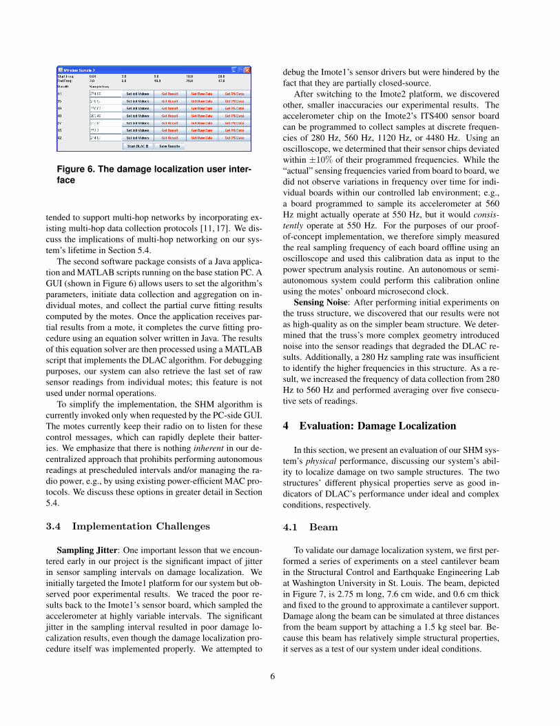
Figure 6. The damage localization user inter-face
tended to support multi-hop networks by incorporating ex-isting multi-hop data collection protocols [11, 17]. We dis-cuss the implications of multi-hop networking on our sys-tem’s lifetime in Section 5.4.
The second software package consists of a Java applica-tion and MATLAB scripts running on the base station PC. AGUI (shown in Figure 6) allows users to set the algorithm’sparameters, initiate data collection and aggregation on in-dividual motes, and collect the partial curve fitting resultscomputed by the motes. Once the application receives par-tial results from a mote, it completes the curve fitting pro-cedure using an equation solver written in Java. The resultsof this equation solver are then processed using a MATLABscript that implements the DLAC algorithm. For debuggingpurposes, our system can also retrieve the last set of rawsensor readings from individual motes; this feature is notused under normal operations.
To simplify the implementation, the SHM algorithm iscurrently invoked only when requested by the PC-side GUI.The motes currently keep their radio on to listen for thesecontrol messages, which can rapidly deplete their batter-ies. We emphasize that there is nothing inherent in our de-centralized approach that prohibits performing autonomousreadings at prescheduled intervals and/or managing the ra-dio power, e.g., by using existing power-efficient MAC pro-tocols. We discuss these options in greater detail in Section5.4.
3.4 Implementation Challenges
Sampling Jitter: One important lesson that we encoun-tered early in our project is the significant impact of jitterin sensor sampling intervals on damage localization. Weinitially targeted the Imote1 platform for our system but ob-served poor experimental results. We traced the poor re-sults back to the Imote1’s sensor board, which sampled theaccelerometer at highly variable intervals. The significantjitter in the sampling interval resulted in poor damage lo-calization results, even though the damage localization pro-cedure itself was implemented properly. We attempted to
debug the Imote1’s sensor drivers but were hindered by thefact that they are partially closed-source.
After switching to the Imote2 platform, we discoveredother, smaller inaccuracies our experimental results. Theaccelerometer chip on the Imote2’s ITS400 sensor boardcan be programmed to collect samples at discrete frequen-cies of 280 Hz, 560 Hz, 1120 Hz, or 4480 Hz. Using anoscilloscope, we determined that their sensor chips deviatedwithin ±10% of their programmed frequencies. While the“actual” sensing frequencies varied from board to board, wedid not observe variations in frequency over time for indi-vidual boards within our controlled lab environment; e.g.,a board programmed to sample its accelerometer at 560Hz might actually operate at 550 Hz, but it would consis-tently operate at 550 Hz. For the purposes of our proof-of-concept implementation, we therefore simply measuredthe real sampling frequency of each board offline using anoscilloscope and used this calibration data as input to thepower spectrum analysis routine. An autonomous or semi-autonomous system could perform this calibration onlineusing the motes’ onboard microsecond clock.
Sensing Noise: After performing initial experiments onthe truss structure, we discovered that our results were notas high-quality as on the simpler beam structure. We deter-mined that the truss’s more complex geometry introducednoise into the sensor readings that degraded the DLAC re-sults. Additionally, a 280 Hz sampling rate was insufficientto identify the higher frequencies in this structure. As a re-sult, we increased the frequency of data collection from 280Hz to 560 Hz and performed averaging over five consecu-tive sets of readings.
4 Evaluation: Damage Localization
In this section, we present an evaluation of our SHM sys-tem’s physical performance, discussing our system’s abil-ity to localize damage on two sample structures. The twostructures’ different physical properties serve as good in-dicators of DLAC’s performance under ideal and complexconditions, respectively.
4.1 Beam
To validate our damage localization system, we first per-formed a series of experiments on a steel cantilever beamin the Structural Control and Earthquake Engineering Labat Washington University in St. Louis. The beam, depictedin Figure 7, is 2.75 m long, 7.6 cm wide, and 0.6 cm thickand fixed to the ground to approximate a cantilever support.Damage along the beam can be simulated at three distancesfrom the beam support by attaching a 1.5 kg steel bar. Be-cause this beam has relatively simple structural properties,it serves as a test of our system under ideal conditions.
6

0.66
m1.
35 m
1.9
m2.
75 m
Wireless SensorDamage Location
Figure 7. Diagram of cantilever beam test struc-ture
Fig 5. Cantilever beam finite element model
Table. 3. Analytical natural frequencies
The first experimental test performed is to experimentally calculate the healthy natural
frequencies of the beam. A hammer strike is applied along the weaker bending axis of the beam
to approximate an impulse response and ensure a total modal content excitation. The first five
healthy natural frequencies, shown in Table 4, are determined by averaging the results from all
of the sensors. Differences between the analytical and experimental healthy natural frequencies
can be explained due to some numerical assumptions in the analytical model. Boundary
conditions, homogeneous distribution for density and constitutive laws, and disregarding
numerical modeling for the sensor platforms are the most important causes for those
discrepancies. However, damage detection results will demonstrate that the DLAC algorithm is
reliable and robust to account for numerical model imperfections even when differences are
large (Clayton, 2006); here the errors range from 18% in the fundamental mode to 0.3% in
higher modes. In general, damage detection algorithms are required to show reliable robustness
to account for numerical model imperfections.
Table 4. Experimental healthy natural frequencies
Mass is then attached to the beam to test the DLAC performance under the three different
scenarios already described. Because the DLAC is used to detect individual events, each
scenario is tested separately. Impact testing is again selected to perform the validation for each
Figure 8. Cantilever beam finite element model
Mode 1 2 3 4 5Measured 0.5381 4.0240 11.4705 22.5506 37.4316Analytical 0.6564 4.1133 11.5180 22.5710 37.3160
Table 1. Measured and analytical natural fre-quencies for the healthy beam
We collected data about the beam’s healthy state by at-taching seven Imote2 wireless sensors at equidistant inter-vals along the beam. Each mote was equipped with a Cross-bow ITS400 sensor board with embedded 3-axis accelerom-eters; tests on a shake table confirmed that these accelerom-eters are sufficiently accurate for DLAC purposes withintheir saturation range of ±2.0g. After exciting the beamwith a hammer, we collected vibration data from each mote.Using this data, we determined the beam’s healthy naturalfrequencies offline, as shown in Table 1.
A corresponding 2D Bernoulli beam model was gener-ated in MATLAB, which subdivided the beam into 20 el-ements with 42 global degrees of freedom (Figure 8). Asshown in Table 1, the first natural frequency predicted bythe model is within 22% of the experimental value, whilethe other predicted frequencies fall within 2% of the exper-imental data. These discrepancies can be explained by sim-plifying assumptions in the model; e.g., the Imote2 nodeswere not included in the model. We remind the reader thatthe DLAC algorithm uses both measured data and analyticaldata as inputs, thus accounting for such discrepancies.
We then tested our system’s ability to detect and local-ize damage along the beam structure. Using the proceduredescribed in Section 3, we collected and analyzed vibra-tion data at 280 Hz, both in its healthy condition and withthe steel bar attached at each of the three damage locations
Mode 1 2 3 4 5Analytical 0.6555 4.0105 10.6192 20.8768 36.1469Sensor 1 0.5506 3.9043 10.2473 20.7641 36.6415Sensor 2 0.5374 3.8902 10.2779 20.8069 36.6396Sensor 3 0.5402 3.8977 10.2714 20.7964 36.6048Sensor 4 0.5316 3.8564 10.2744 20.8470 36.6785Sensor 5 0.5371 3.7678 10.0707 20.4038 36.9797Sensor 6 0.5427 3.8488 10.3217 20.7546 36.5919Sensor 7 0.5392 3.9012 10.2533 20.7751 36.6570
Table 2. Analytical and identified natural fre-quencies for the damaged beam
damage case by applying a hammer strike along the weaker bending axis. Results reported using
the entire network are depicted in Figs. 6, 7 and 8 where corresponding identified natural
frequencies and DLAC measurements are introduced for each damage scenario. DLAC values
determined at sensors along the length of the beam are provided. Values close to unity indicate
damage location. The entire network report successful damage detection results for all damage
scenarios with correlation measurements greater than 90% at the damaged positions. Recall
experimental damage positions D1, D2 and D3 are associated with elements 5, 10 and 14,
respectively. Despite consistency in the results, some of the sensors report correlation
measurements greater than 50% for some of the element positions. As explained previously,
results of correlation-based methods may not be unique. Frequency change vectors associated
with one damage location could be potentially the same as those obtained with several
combinations of damage location when reduced numbers of modes are used. Therefore, the
inclusion of more modes is expected to clarify the results by concentrating the correlation
measurements around one damage location. Note that these results are obtained with a damage
hypothesis of only 67% of the actual damage. Two additional damage hypotheses are
implemented to test the DLAC performance off-line using different damage assumptions and
acceleration records previously obtained for debugging purposes. New sensitivities matrices and
corresponding frequency change vectors were developed with a prescribed analytical damages
equivalent to 200% and 33% of the actual damage. Results showed the same tendencies and
consistency, and were also successful for all damage scenarios with high correlation
measurements.
Fig 6. DLAC results for element position # 5
0 10 200
0.1
0.2
0.3
0.4
0.5
0.6
0.7
0.8
0.9
1
X = 5
Y = 0.94
DLAC WS1
Element Position
0 10 200
0.1
0.2
0.3
0.4
0.5
0.6
0.7
0.8
0.9
1
X = 5
Y = 0.971
DLAC WS2
Element Position
0 10 200
0.1
0.2
0.3
0.4
0.5
0.6
0.7
0.8
0.9
1
X = 5
Y = 0.972
DLAC WS3
Element Position
0 10 200
0.1
0.2
0.3
0.4
0.5
0.6
0.7
0.8
0.9
1
X = 5
Y = 0.955
DLAC WS4
Element Position
0 10 200
0.1
0.2
0.3
0.4
0.5
0.6
0.7
0.8
0.9
1
X = 5
Y = 0.964
DLAC WS5
Element Position
0 10 200
0.1
0.2
0.3
0.4
0.5
0.6
0.7
0.8
0.9
1
X = 5
Y = 0.965
DLAC WS6
Element Position
0 10 200
0.1
0.2
0.3
0.4
0.5
0.6
0.7
0.8
0.9
1
X = 5
Y = 0.97
DLAC WS7
Element Position
Figure 9. DLAC results for the beam damagedat element 5
7

shown in Figure 7. We added an arbitrary amount of mass ateach position in our analytical model to develop the matrixof damage cases for computation of the correlation factors.The amount of mass that we added to the model intention-ally did not match the steel bar’s actual mass. We includedthis discrepancy to reflect the fact that the amount of dam-age to a structure is not known ahead-of-time, and to il-lustrate that DLAC will still adequately localize damage aslong as a reasonable guess is used.
For the sake of brevity, we present here only the resultsfor the first scenario, which simulates damage at the beam’sfifth element. As shown in Table 2, the natural frequenciesmeasured by each of the 7 sensor nodes closely match thosepredicted by the “damaged” analytical model. Each nodetherefore correctly predicts structural damage at the beam’sfifth element with a correlation of 94% or higher (Figure 9).We observed similar results during the other two damagescenarios, with the nodes consistently localizing the damageat the correct element with correlations of 90% or higher.
Figure 10. 3D truss test structure
Wireless SensorTruss Frontal Panel
Figure 11. Truss experimental setup; high-lighted elements were replaced to simulatedamage
4.2 Truss
To evaluate our system under more complex structuralconfigurations, we then performed tests on a 5.6 m steeltruss structure [6] at the Smart Structure Technology Lab-oratory (SSTL) at the University of Illinois at Urbana-
Mode 1 2 3 4 5Measured 20.65 41.49 64.59 69.41 95.51Analytical 19.88 38.31 66.26 67.17 92.25
Table 3. Measured and analytical natural fre-quencies for the healthy truss
Mode 1 2 3 4 5Analytical 19.19 38.35 63.58 66.30 90.96Sensor 1 20.27 41.37 63.04 67.79 94.89Sensor 2 20.28 41.40 63.17 67.89 95.08Sensor 3 20.20 41.29 63.01 67.67 94.82Sensor 4 20.17 41.23 63.05 67.68 94.73Sensor 5 20.31 41.30 63.10 67.73 94.89Sensor 6 20.23 41.29 63.02 67.68 94.81
Table 4. Analytical and identified natural fre-quencies for the damaged truss
Champaign (see Figure 10). 11 Imote2 sensors were de-ployed on the frontal panel of the truss, as shown in Fig-ure 11; USB cabling was deployed to power the motes, butall communication occurred over their wireless radios. Thetruss consists of fourteen bays 0.4 m-long bays and sits onfour rigid supports. Different structural configurations anddamage scenarios can be emulated by removing or replac-ing the truss’s members and its supports.
As with the beam, we used collected truth data and aMATLAB model to compute the natural frequencies in thetruss’s healthy state. We collected the truth data by verti-cally exciting the truss structure using a magnetic shaker.(To ensure a consistent mass distribution with later exper-iments, the Imote2 motes were left installed but were notactivated.) A force transducer was used to measure the in-put force, and six wired sensors were used to measure thevibrations at different points on the truss’s frontal panel.A corresponding numerical finite element model with 160beam elements and 336 global degrees of freedom (Figure12) was generated in MATLAB. As shown in Table 3, thenatural frequencies predicted by this model are within 2–7%of the experimental data. Again, these discrepancies can beexplained by simplifying assumptions in the model and areaccommodated by the DLAC algorithm.
Figure 12. Truss finite element model
8

To simulate damage along the truss structure, we re-placed the beam elements of the third bay (highlighted inFigure 11) with smaller elements. Specifically, two diago-nal elements were reduced in area by 52.7%, and two bot-tom elements were reduced in area by 63.7%. We simu-lated damage to the truss’s numerical model by reducingthe model’s corresponding beam elements.
Fig 12. DLAC results for truss bay # 3
6.0 CONCLUSIONS
In this study a successful demonstration for an in-situ experimental validation of a
correlation-based decentralized damage detection technique using a wireless sensor network has
been performed. Structural damage was detected with sufficiently high correlation percentage in
two experimental structures independently of the damage hypothesis used in the sensitivity
matrix. On-board processing iMote2 capacities were exploited to reduce communication load
and make the application scalable within a wireless sensor network.
7.0 ACKNOWLEDGMENT S
Funding for this research is provided in part by the National Science Foundation; grant NSF
NeTS-NOSS Grant CNS-0627126, by Washington University in St. Louis. Additionally, the
authors would like to thank Prof. Bill Spencer and Shin-Ae Jang for the use of and assistance
with the experimental truss.
8.0 REFERENCES
Clayton, E.H. (2002), “Development of an Experimental Model for the Study of Infrastructure
Preservation”, Proceedings of the National Conference on Undergraduate Research,
Whitewater, Wisconsin.
Clayton, E.H., Koh, B.H., Xing, G., Fok, C.L., Dyke, S.J. and Lu, C. (2005), “Damage
Detection and Correlation-based Localization Using Wireless Mote Sensors”, Proceedings
of ’05 The 13Th
Mediterranean Conference on Control and Automation, Limassol, Cyprus.
Clayton, E.H. (2006), “ Frequency Correlation-based Structural Health Monitoring with Smart
Wireless Sensors”, Master of Science Thesis, Washington University in St. Louis.
1234567891011120
0.1
0.2
0.3
0.4
0.5
0.6
0.7
0.8
0.9
1
X = 3Y = 0.868
DLAC WS #32
Truss Central Bay Position
1234567891011120
0.1
0.2
0.3
0.4
0.5
0.6
0.7
0.8
0.9
1
X = 3Y = 0.864
DLAC WS #45
Truss Central Bay Position
1234567891011120
0.1
0.2
0.3
0.4
0.5
0.6
0.7
0.8
0.9
1
X = 3Y = 0.871
DLAC WS #67
Truss Central Bay Position
1234567891011120
0.1
0.2
0.3
0.4
0.5
0.6
0.7
0.8
0.9
1
X = 3Y = 0.873
DLAC WS #28
Truss Central Bay Position
1234567891011120
0.1
0.2
0.3
0.4
0.5
0.6
0.7
0.8
0.9
1
X = 3Y = 0.825
DLAC WS #35
Truss Central Bay Position
1234567891011120
0.1
0.2
0.3
0.4
0.5
0.6
0.7
0.8
0.9
1
X = 3Y = 0.865
DLAC WS #75
Truss Central Bay Position
Figure 13. DLAC results for the damagedtruss
We then excited the “damaged” truss structure and usedthe Imote2 nodes to collect vibration data. Because the trusshas more complex behavior than the beam, we increasedthe sampling frequency to 560 Hz. To reduce noise, wealso averaged the power spectrum results over five consec-utive readings. 6 of the 11 sensors reported enough vibra-tion data2 to compute natural frequencies with a DLAC cor-relation of 85%. The natural frequency data and DLACresults are shown in Table 4 and Figure 13, respectively.The DLAC results strongly predict damage in the third bay,which is where the elements were replaced.
5 Evaluation: Feasibility and Advantages
We now evaluate the cyber aspects of our cyber-physicalSHM system. Specifically, we demonstrate that our pro-totype application’s memory, computational, and energyrequirements all fall within the capabilities of current-generation sensor network hardware. We also show that oursystem significantly outperforms a centralized approach interms of latency and energy requirements. Based on thesefindings, we project that our system would achieve a life-time of approximately 191 days between battery replace-ments with appropriate power management techniques. In
2The Imote2 vibration sensor will occasionally fail to collect a roundof samples, due to a driver bug that could not be isolated by the time theexperiments were run.
Type Size Fraction of Imote2capacity
ROM 248172 bytes 0.74%RAM (heap) 63588 bytes
0.22%RAM (stack) 9126 bytes
Table 5. The ROM and RAM footprint of theSHM application
the interest of brevity, we will only discuss here the effectsof partitioning our decentralized application in the way de-scribed in Section 3.2. Readers may find a performancecomparison of different partitioning schemes in [13].
5.1 Memory
We present the RAM consumption of the entire WSNcomponent of the system when compiled for the Imote2platform in Table 5 along with its ROM footprint. TheseROM and RAM requirements are well within the capacityof current-generation mote hardware. Indeed, on platformssuch as the Imote2 (which is equipped with 32 MB eachof flash ROM and SDRAM) this application would signifi-cantly underutilize the hardware capabilities.
0 2000 4000 6000 8000 10000 12000 14000Latency (ms)
Decentralized
Centralized
SamplingComputationCommunication
Figure 14. The latency of sensor data collec-tion and aggregation
5.2 Latency
To evaluate the latency of a single round of damage lo-calization, we timed the execution of the round’s five stages:collecting raw sensor from the accelerometer, computingthe FFT of the raw data, performing power spectrum anal-ysis on the transformed data, constructing the matrix forroot detection, and transmitting the matrix coefficients tothe base station. For the purposes of comparison, we alsomeasured the latency of transmitting all 2048 raw sensorreadings back to the base station for centralized process-ing. Where possible, we measured these latencies using theImote2’s onboard microsecond timer and took the mean of50 rounds. Because the Imote2’s onboard radio interfereswith the hardware microsecond timer, the data transmissionlatencies were collected over 10 rounds using an oscillo-scope. We focus here on the latencies incurred by on-board
9

processing and communication, excluding processing at thebase station. We note that this decision benefits the cen-tralized approach, which will pay a comparatively higherprocessing cost at the base station.
Figure 14 presents the average latency for the decen-tralized algorithm (which performs computation locally andonly transmits the matrix coefficients) and a centralized ap-proach (which performs no computation but transmits allraw sensor readings). For the purposes of legibility, we havegrouped the FFT, power spectrum analysis, and root detec-tion stages together into a single computation stage.
Both the centralized and the decentralized schemes incura mean cost of 3772 ms (σ = 0.80 ms) to collect raw sen-sor data. This closely matches the 2048
560 Hz ≈ 3.7 s neededto collect 2048 samples, with some additional overhead tocopy the sensor data into a local buffer. The decentralizedapproach incurs a mean 681 ms latency (σ = 2.79 ms) for itscomputation stage which the centralized approach does notneed. However, the data aggregation performed in this stagereduces the data to be transmitted by 98.8%, from 2048 datapoints to 25. Therefore, the decentralized scheme takes only270 ms (σ = 10 ms) to transmit the computed coefficients tothe base station, whereas the centralized approach requires9638 ms (σ = 28 ms) to transmit its raw data.
By performing computation and aggregation on thenodes, we incur very little system overhead on our current-generation sensor hardware. 77.4% of the system’s timeis spent collecting data; only 22.6% of the latency repre-sents reducible overhead. In comparison, the centralizedapproach spends 71.9% of its time transmitting data to thebase station. As a result, our decentralized system canachieve latencies 64.8% lower than those of a centralizedalgorithm.
0.00 0.05 0.10 0.15 0.20 0.25Energy Consumption (mAh)
Decentralized
Centralized
SamplingComputationCommunication
Figure 15. The energy consumption of sensordata collection and aggregation
5.3 Energy Consumption
The current version of our SHM system performs onlylimited power management, since the TinyOS 1.1 driversfor the Imote2 do not put all of the hardware to sleep whendeactivated. As of this writing, the Imote2 driver subsys-tem is being rewritten for TinyOS 2, which we expect tofix this shortcoming. Nevertheless, we can estimate the en-
ergy consumption of a fully power-managing SHM systemby combining the latency statistics given above with currentconsumption data for the radio, sensor, and CPU taken fromthe corresponding datasheets [9, 31, 34].
Figure 15 shows the energy cost of a single round ofSHM data collection. Our decentralized solution signifi-cantly reduces energy consumption compared to a central-ized approach, from 0.222 mAh to 0.067 mAh. This re-duction is mainly due to the expense of sending raw sen-sor readings to the base station. The decentralized approachconsumes 0.006 mAh (31 mA [9] for 681 ms) to perform itscomputations. However, this computation saves the mote anaverage of 0.160 mAh during transmission, since it reducesthe time that the radio is active and transmitting by 9367ms.
1 reading/week 1 reading/day 1 reading/hour0
50
100
150
200
250
Pro
ject
ed lifeti
me (
days)
DecentralizedCentralizedDecentralized(0.1% duty cycle)
Centralized(0.1% duty cycle)
Figure 16. System lifetime under different us-age patterns
5.4 Projected Lifetime
We can estimate the system’s expected lifetime by notingthat the Imote2 consumes 382 µA in its deep sleep state [9],plus 15 µA for the accelerometer [31]. Figure 16 presentsthe estimated system lifetime when the Imote2 is deployedwith a standard 3x AAA battery pack providing 2400 mAhof charge. If we assume that the system remains asleep be-tween periodic readings, then the decentralized approachachieves a projected lifetime of 213 days, even at a rela-tively aggressive hourly schedule. In contrast, the central-ized approach achieves a lifetime of 160 days at an hourlyschedule, though it stays within 2% of the decentralized ap-proach’s lifetime at lower frequencies. The sharp drop in thecentralized system’s lifetime occurs because sleeping dom-inates the system’s energy cost at lower frequencies, whilethe high communications costs dwarf the sleeping cost atan hourly frequency. As a result, in-situ processing enablesmore frequent monitoring than is realistically possible for acentralized scheme.
10
In practice, a SHM system may not be able to behave au-tonomously: its deployers may want some kind of manualcontrol (e.g., to perform on-demand readings after a nat-ural disaster). This can be achieved by having the nodeslisten for radio transmissions between readings. Keepingthe CPU and radio active at 100% duty cycles would reducethe node lifetime to only 55 hours. However, power-savingMAC layers like SCP [36] can achieve duty cycles as low as0.1% with reasonable responsiveness tradeoffs. As shownin Figure 16, this would have a fairly low impact on sys-tem lifetime (an 8.5%–9.8% reduction in the decentralizedcase).
0 10 20 30 40 50# of hops
60
80
100
120
140
160
180
200
Pro
ject
ed lifeti
me (
days)
DecentralizedCentralized
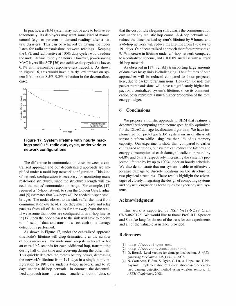
Figure 17. System lifetime with hourly read-ings and 0.1% radio duty cycle, under variousnetwork configurations
The difference in communication costs between a cen-tralized approach and our decentralized approach are am-plified under a multi-hop network configuration. This kindof network configuration is necessary for monitoring manyreal-world structures, since the structure’s length will ex-ceed the motes’ communication range. For example, [17]required a 46-hop network to span the Golden Gate Bridge,and [5] estimates that 3–4 hops will be needed to span smallbridges. The nodes closest to the sink suffer the most fromcommunication overhead, since they must receive and relaypackets from all of the nodes further away from the sink.If we assume that nodes are configured in an n-hop line, asin [17], then the node closest to the sink will have to receiven − 1 sets of data and transmit n sets each time damagedetection is performed.
As shown in Figure 17, under the centralized approachthis node’s lifetime will drop dramatically as the numberof hops increases. The mote must keep its radio active foran extra 19.2 seconds for each additional hop, transmittingduring half of this time and receiving during the other half.This quickly depletes the mote’s battery power, decreasingthe network’s lifetime from 191 days in a single-hop con-figuration to 180 days under a 4-hop network, and to 95days under a 46-hop network. In contrast, the decentral-ized approach transmits a much smaller amount of data, so
that the cost of idle sleeping still dwarfs the communicationcost under any realistic hop count. A 4-hop network willreduce the decentralized system’s lifetime by 9 hours, anda 46-hop network will reduce the lifetime from 196 days to191 days. Our decentralized approach therefore represents a9.1% increase in lifetime under a 4-hop network comparedto a centralized scheme, and a 100.0% increase with a larger46-hop network.
As observed in [17], reliably transporting large amountsof data over lossy links is challenging. The lifetimes of bothapproaches will be reduced compared to those projectedhere, due to packet retransmissions. However, we note thatpacket retransmissions will have a significantly higher im-pact on a centralized system’s lifetime, since its communi-cation costs represent a much higher proportion of the totalenergy budget.
6 Conclusions
We propose a holistic approach to SHM that features adecentralized computing architecture specifically optimizedfor the DLAC damage localization algorithm. We have im-plemented our prototype SHM system on an off-the-shelfsensor platform while using less than 1% of its memorycapacity. Our experiments show that, compared to earliercentralized solutions, our system can reduce the latency andenergy consumption of each damage localization round by64.8% and 69.5% respectively, increasing the system’s pro-jected lifetime by by up to 100% under an hourly schedule.We also demonstrate that our system is able to effectivelylocalize damage to discrete locations on the structure ontwo physical structures. These results highlight the advan-tages of closely integrating the design of computing systemsand physical engineering techniques for cyber-physical sys-tems.
Acknowledgment
This work is supported by NSF NeTS-NOSS GrantCNS-0627126. We would like to thank Prof. B.F. Spencerand Shin Ae Jang for the use of the truss for our experimentsand all of the valuable assistance provided.
References
[1] http://www.tinyos.net.[2] http://www.cse.wustl.edu/wsn.[3] D. Bernal. Load vectors for damage localization. J. of En-
gineering Mechanics, 128(1):7–14, 2002.[4] N. Castaneda, F. Sun, S. Dyke, C. Lu, A. Hope, and T. Na-
gayama. Implementation of a correlation-based decentral-ized damage detection method using wireless sensors. InASEM Conference, 2008.
11

[5] K. Chebrolu, B. Raman, N. Mishra, P. K. Valiveti, andR. Kumar. BriMon: a sensor network system for railwaybridge monitoring. In MobiSys, 2008.
[6] E. Clayton. Development of an experimental model for thestudy of infrastructure preservation. Proc. of the NationalConference on Undergraduate Research, Whitewater, Wis-consin, 2002.
[7] E. Clayton. Frequency correlation-based structural healthmonitoring with smart wireless sensors. Master’s thesis,Washington University in St. Louis, 2006.
[8] Crossbow Technology, Inc. ITS400 Imote2 Basic SensorBoard.
[9] Crossbow Technology, Inc. Imote2 Hardware ReferenceManual, 2007.
[10] C. Farrar, D. Allen, G. Park, S. Ball, and M. Masque-lier. Coupling sensing hardware with data interrogation soft-ware for structural health monitoring. Shock and Vibration,13(4):519–530, 2006.
[11] R. Fonseca, O. Gnawali, K. Jamieson, S. Kim, P. Levis, andA. Woo. The collection tree protocol (CTP).
[12] Y. Gao. Structural Health Monitoring Strategies for SmartSensor Networks. PhD thesis, University of Illinois atUrbana-Champaign, 2005.
[13] G. Hackmann, F. Sun, N. Castaneda, C. Lu, and S. Dyke.A holistic approach to decentralized structural damage lo-calization using wireless sensor networks. Technical ReportWUCSE-2008-9, Washington University in St. Louis, 2008.
[14] J. Juang and R. Pappa. An eigensystem realization algorithmfor modal parameter identification and model reduction. J.of Guidance Control and Dyn., 8:620–627, 1985.
[15] S. Kim. Wireless sensor networks for structural health mon-itoring. Master’s thesis, University of California at Berkeley,2005.
[16] S. Kim. Wireless Sensor Networks for High Fidelity Sam-pling. PhD thesis, University of California at Berkeley,2007.
[17] S. Kim, S. Pakzad, D. Culler, J. Demmel, G. Fenves,S. Glaser, and M. Turon. Health monitoring of civil infras-tructures using wireless sensor networks. In IPSN, 2007.
[18] A. Kiremidjian, E. Straser, T. Meng, K. Law, and H. Sohn.Structural damage monitoring for civil structures. Proc. ofInt. Workshop on Structural Health Monitoring, Stanford,CA., pages 371–382, 1997.
[19] E. C. Levy. Complex-curve fitting. IRE Transactions onAutomatic Control, 4:37–44, 1959.
[20] S. Liu and M. Tomizuka. Strategic research for sensors andsmart structures technology. Proc. of the International Con-ference on Structural Health Monitoring and Intelligent In-frastructure, Tokyo, Japan, 1:113–117, 2003.
[21] S. Liu and M. Tomizuka. Vision and strategy for sensors andsmart structures technology research. Proc. of the 4th Inter-national Workshop on Structural Health Monitoring, Stan-ford, CA, pages 15–17, 42–52, 2003.
[22] J. Lynch. Overview of wireless sensors for real time healthmonitoring of civil structures. Proc. of the 4th InternationalWorkshop on Structural Control, pages 189–194, 2004.
[23] J. Lynch and K. Loh. A summary review of wireless sensorsand sensor networks for structural health monitoring. Shockand Vibration Digest, 38(2):91–128, 2006.
[24] A. Messina, I. A. Jones, and E. J. Williams. Damage de-tection and localization using natural frequency changes. InConference on Identification in Engineering Systems, U.K.,1996.
[25] A. Messina, E. J. Williams, and T. Contursi. Structural dam-age detection by a sensitivity and statistical-based method.Journal of Sound and Vibration, 215(5):791–808, 1998.
[26] J. Paek, K. Chintalapudi, R. Govindan, J. Caffrey, andS. Masri. A wireless sensor network for structural healthmonitoring: performance and experience. In EmNets, 2005.
[27] S. N. Pakzad, G. L. Fenves, S. Kim, and D. E. Culler. Designand implementation of scalable wireless sensor network forstructural monitoring. ASCE Journal of Infrastructure Engi-neering, 14(1):89–101, March 2008.
[28] H. Sohn, C. Farrar, F. Hemez, D. Shunk, D. Stinemates, andB. Nadler. A review of structural health monitoring liter-ature: 1996–2001. Technical Report LA-13976-MS, LosAlamos National Laboratory, 2004.
[29] B. Spencer and T. Nagayama. Smart sensor technology:a new paradigm for structural health monitoring. Proc.of Asia-Pacific Workshop on Structural health Monitoring,Yokohama, Japan., 2006.
[30] B. Spencer, M. Ruiz-Sandoval, and N. Kurata. Smart sens-ing technology: Opportunities and challenges. StructuralControl and Health Monitoring, 11(4):349–368, 2004.
[31] STMicroelectronics. LIS3L02DQ MEMS Inertial Sensor,2005.
[32] E. Straser and A. Kiremidjian. A modular visual approachto damage monitoring for civil structures. Proc. of SPIE:Smart Structures and Materials, pages 112–122, 1996.
[33] E. Straser and A. Kiremidjian. A modular, wireless damagemonitoring system for structures. Technical report, The JohnA. Blume Earthquake Engineering Center, 1998.
[34] Texas Instruments. 2.4 GHz IEEE 802.15.4 / ZigBee-readyRF Transceiver.
[35] N. Xu, S. Rangwala, K. Chintalapudi, D. Ganesan,A. Broad, R. Govindan, and D. Estrin. A wireless sensornetwork for structural monitoring. In SenSys, 2004.
[36] W. Ye, F. Silva, and J. Heidemann. Ultra-low duty cycleMAC with scheduled channel polling. In SenSys, 2006.
12