A Holistic Approach for the Generic Preliminary Design of

A HOLISTIC APPROACH FOR THE GENERIC PRELIMINARY DESIGN OF AXIAL COMPRESSOR AND TURBINE ANNULUS CONTOURS

M. Mischke*, M. Pohl*, K. Höschler*, A. Huppertz** * Brandenburg University of Technology Cottbus-Senftenberg, 03046 Cottbus, Germany ** Rolls-Royce Deutschland Ltd. & Co KG, 15827 Blankenfelde-Mahlow, Germany

Abstract

An essential aspect in the whole engine modelling of modern aircraft engines is the preliminary design of the meridional gas path definition. Especially the annulus dimensioning and topological characterisation of engine core subsystems are usually time-consuming. This paper presents a holistic and parametric approach to pre-design the geometric 2D annulus contours of compressor and turbine subsystems without complex thermody-namic calculations. It is based on distribution functions of the axial and radial dimensions, as well as the vari-ations of compressor and turbine stages and realises a time-efficient re-dimensioning and topological variation of the complex annulus geometry. Parametric methods for an optimised arrangement of the blade stages in a turbomachinery subsystem configuration are shown and integrated into a mathematical model.

Keywords: Gas Path; Annulus Contour; Generic Preliminary Design; Turbine; Compressor

NOMENCLATURE

HPT High Pressure Turbine H Hubline

LPT Low Pressure Turbine LE Leading Edge

L axial length TE Trailing Edge

A area, cross section � index of the last stage in a configuration

P 2D-point in meridional plane {x; r} �, �, � index of an arbitrary position in a config.

x axial component ∆ difference between two values

r radial component � percentage of a total value

C component (R, S or G) ~ normalised value

R rotor ∇, gradient of a line segment

S stator �� normalised function, distribution function

G gap (passage between R/S or S/R) �, , �, factor

T Tipline (casing line)

1. INTRODUCTION

The generation and preliminary design of the gas path structure (annulus contour) are essential objec-tives during the development of modern aircraft en-gines. The basic subsystems compressor, combus-tion chamber and turbine mainly describe the gas path of a core engine. In general, the swan-neck duct and the LPT diffuser are included in the annulus ge-ometry [1–3]. The dimensioning of the gas path and the topological pre-design in the compressor and tur-bine subsystems are particularly time-consuming and extremely computationally intensive.

Therefore, the pre-design and optimisation of com-pressor and turbine configurations are constantly in focus in the field of research and development of aero turbo-engines. Many of these investigations, like the work of Agromayor et al. [4], Keskin [5] and Sommer [6], deal with the three-dimensional geometric and topological design of system-internal geometries such as the rotor and stator blades. However, these methods also require basic input data, which can only be derived from the two-dimensional shape of the an-nulus contour. Hence, a corresponding pre-definition of the space-limiting annulus geometry is necessary.

doi:10.25967/530097CC BY 4.0

Deutscher Luft- und Raumfahrtkongress 2020DocumentID: 530097

1

https://creativecommons.org/licenses/by/4.0/

https://doi.org/10.25967/530097

For this purpose, modern optimisation strategies can be applied to determine the design of the tur-bomachinery subsystems and the resulting gas path contour. This basic contour can be generated from scratch by a multitude of iterations [7,8]. However, de-pending on the complexity of the algorithm and due to ambiguous initial values, numerous possible gas path designs can be lost. By providing a precondi-tioned annulus contour, the number of iterations can be reduced significantly, because the optimisation process only has to adjust the annulus contour in-stead of creating it from scratch. Hendler et al. [9] show a method for adjusting the overall gas path con-tour of several combined subsystems. The complex optimisation procedure also requires a suitable initial geometry, as well as predefined optimisation targets and parameters, which are fed into the process.

When defining automated process sequences using optimisation algorithms, it is usually necessary to pa-rameterise the required design variables instead to vary them directly. For particularly complex systems it can be necessary to reduce the mathematical de-sign space. This can be achieved by a simplified but sufficiently accurate or even dimensionless parame-terisation of the considered system. In his work on process acceleration of compressor optimisation Hinz [10] presents a first approach of a time-efficient strat-egy for the axial distribution of rotor and stator com-ponents in the compressor system. Resultant, Hinz derived a simplified parameterisation of the axial ex-pansions of compressor components for subsequent 2D optimisation strategies.

Based on this, a holistic approach for a time-efficient preliminary design generation of the subsystem com-ponent annulus contour is realised in this paper. The two-dimensional design of the rotor and stator stages are represented by aeroblocks. These objects define the precise axial and radial position and dimensioning of any stages in the designed gas path. The specific adjustments of the input parameters, in combination with the analysis of normalised distribution functions for the geometric dimensioning and topological varia-tion of the aeroblocks, provides the potential of this work to calculate a large number of possible geomet-ric annulus contours in a minimum of time.

2. BASIC CONCIDERATIONS

2.1. Curves and Splines as design tool

Since the development of the aircraft turbo-engine by Prof. Dr. H.-J. Pabst v. Ohain (1937) and Sir F. Whit-tle (1939) [2,3], the efforts to describe aircraft engine subsystem components using an approach of defined

parametric calculations have to become indispensa-ble. A uniform theory of compressor design was pub-lished in 1942 by Traupel [11]. Based on this theory, P. de Haller [12] and S. J. Andrews et al. [13] worked out their studies, to verify the influence of parameters in compressor blade design with test results. This idea of a parameterised engine design has been con-tinuously expanded over the decades. With the estab-lishment of more powerful computer technology, the parameterised engine design finally led to the field of mechanical system optimisation.

The early approaches of general parameterisation strategies of structures comes from the field of typog-raphy. As early as 1517, Torniello et al. [14] made the first efforts to describe letters mathematically using straight lines and circles. Weierstrass (1885) achieved an important milestone by proving the ap-proximation of real continuous functions on a real, limited and closed area using polynomials. This poly-nomial approach was taken up by Bernstein in 1912 and led to the general theory of Bernstein Polynomi-als [15]. In 1958 P. F. de Casteljau (Citroën) and P. Bézier (Renault) used the Bernstein Polynomials to calculate free-form curves in car body design [16]. The approach developed by Bezier was published in 1960 under the name "Bezier-Curves". The further development of parameterised curves by C. de Boor, I. J. Schoenberg and Hiroshi Akima to the well known Splines, B-Splines and Akima-Splines should not re-main unmentioned, but will not be further discussed in this work.

2.2. Thermodynamic conditions and constraints

A precondition for the generic gas path approach of axial turbo-engines is the knowledge of some geo-metric and topological system variables of the consid-ered subsystem component. In order to comply with the character of a time-efficient preliminary design, these variables are limited to

the axial length (�), the number of stages (�), and the area of the inlet and outlet cross sec-

tion (��)

in the system to be designed (Fig. 1). Depending on the level of detail, the system length (�) and the num-ber of stages (�) can be specified. The required inlet- and outlet cross sections can be calculated using sim-ple synthesis-based calculation methods for engine pre-dimensioning [2,3] or by much more complex nu-merical approaches. The following calculation ap-

CC BY 4.0

Deutscher Luft- und Raumfahrtkongress 2020

2


proaches are presented in general terms and illus-trated by the example of a representative high- and low-pressure turbine.

2.3. Parametrisation of geometric subsystem

components: Point approach

The overall radial change of height of the considered subsystem component can be calculated according to Equation 2.01. For this purpose the absolute value of the difference between the radial values of inlet and

outlet cross section or the point ��,��,� of the last rotor

/ stator stage and the point ��,��,� of the first rotor / sta-

tor stage will be determined.

2.01 ∆�� !" # $�(%&'() ) �(%+,)$ # $��,��,� ) ��,��,�$

∀� ∈/01

The indexing "�" indicates the last component of the last stage. Note that turbine systems, unlike compres-sor systems, usually start with a stator stage and end with a rotor stage. An arbitrary stage position in the considered subsystem is described with the index �, where � # 1, . . . , � ; �˄� ∈ ℕ describes the entire sys-tem arrangement and sets up the quantity of stator-rotor combinations.

The local radial annulus variation within a stage com-ponent 7� can be set up analogous to Equation 2.01 for any rotor or stator stage according to Equation 2.02.

2.02 ∆�� # |��,��,� ) ��,��,�| The total radial extent of all rotors or stators of a sub-system component (7 #9 /, :) is determined by Equa-tion 2.03, by the sum of the individual radial variations of the considered components.

2.03 ∆�� # ; ∆��

�<�

When calculating the radial parts of the individual components, it must be taken into account that each rotor and stator arrangement is followed by a corre-sponding axial gap. Those also causes radial changes in the annulus contour on Hub- and Tipline. Depending on the axial position in the subsystem, there is a distinction between a "rotor to stator" gap or a "stator to rotor" gap (Eq. 2.04). In addition, it must be decided whether the radial gap behind the last ro-tor or stator stage (�) should still be counted as part of the considered subsystem or not (Eq. 2.05).

2.04 ∆��=>/@ # |��,��,� ) ��,��A,�| ; ∆��=@/> # |��,��A,� ) ��,��,�| 2.05 ∆��=>/@ #? 0 ; ∆��=@/> #? 0

After all components have been subdivided and their shares of the overall radial difference within the con-sidered subsystem have been established, Equation

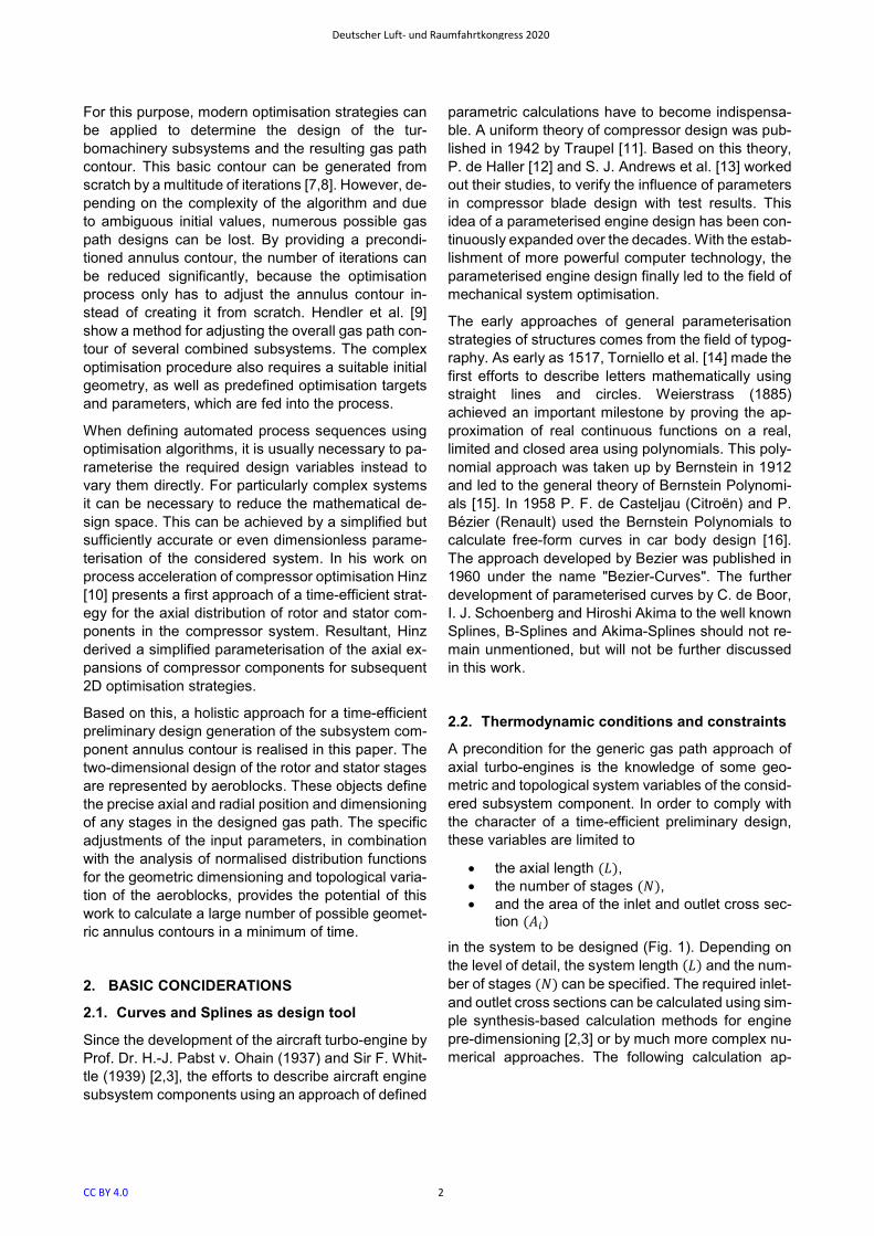
Figure 1: Representative turbine configuration (HPT + LPT) with aeroblocks and parameter definition.

CC BY 4.0


3


2.06 can be used to come a full circle to the initially established Equation 2.01.

2.06

∆�� !" #! ∆�� E ∆�=@/> E ∆�A E ∆�=>/@

#! ;(∆�� E ∆��=@/> E ∆��A E ∆��=>/@)��<�

2.4. Normalisation of subsystem components

Subsequently a normalisation and the associated nondimensionalisation of the geometric and topologi-cal dimensions will be performed. For this purpose, all radial point coordinates are related to the overall ra-dial difference of the considered partial component according to Equation 2.07.

2.07 �̃� # ��∆�� ∈ G0,1H, �� ∈ G�1,�I7,J , ∆��H

For a complete dimensionless description of the sub-system, it is necessary to normalise the previously defined number of stages. As can be seen in Equa-tion 2.08, the arbitrary stage � is related to the total number of stages �.

2.08 K̃ # �� ∈ G0, 1H, � ∈ G1, �H The result of the normalisation represents a graph (distribution function), which describes the depend-ency between the normalised radial variation and the associated normalised stage number of the respec-tive subsystem component. This dependency which, is graphically shown in Figure 2, can be described by Equation 2.09. By varying the indexing, Equation 2.07 and 2.09 can be used for the normalised description

of the radial variation within the axial gaps between rotor to stator or stator to rotor.

2.09 �̃�� # �̃�(K̃) # �̃� L ��M

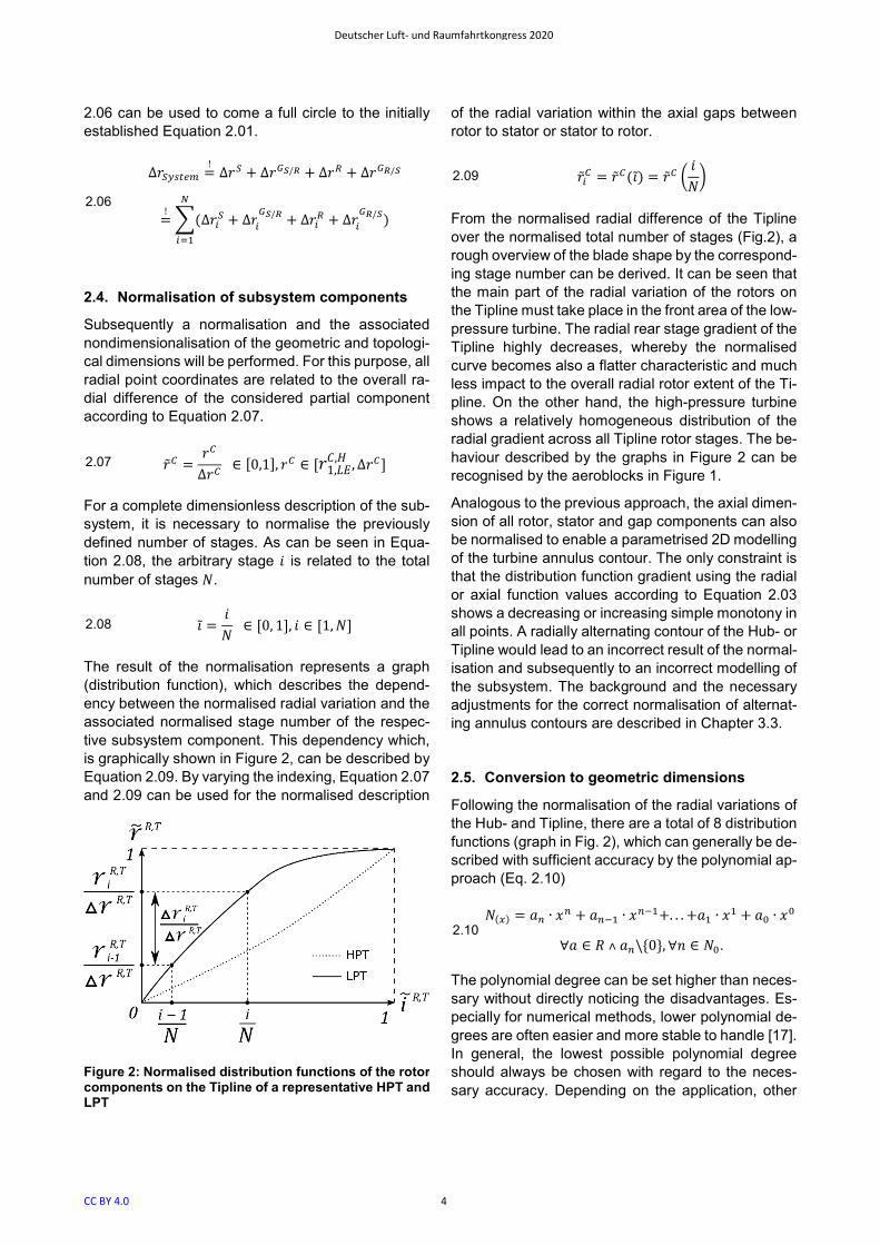
From the normalised radial difference of the Tipline over the normalised total number of stages (Fig.2), a rough overview of the blade shape by the correspond-ing stage number can be derived. It can be seen that the main part of the radial variation of the rotors on the Tipline must take place in the front area of the low-pressure turbine. The radial rear stage gradient of the Tipline highly decreases, whereby the normalised curve becomes also a flatter characteristic and much less impact to the overall radial rotor extent of the Ti-pline. On the other hand, the high-pressure turbine shows a relatively homogeneous distribution of the radial gradient across all Tipline rotor stages. The be-haviour described by the graphs in Figure 2 can be recognised by the aeroblocks in Figure 1.

Analogous to the previous approach, the axial dimen-sion of all rotor, stator and gap components can also be normalised to enable a parametrised 2D modelling of the turbine annulus contour. The only constraint is that the distribution function gradient using the radial or axial function values according to Equation 2.03 shows a decreasing or increasing simple monotony in all points. A radially alternating contour of the Hub- or Tipline would lead to an incorrect result of the normal-isation and subsequently to an incorrect modelling of the subsystem. The background and the necessary adjustments for the correct normalisation of alternat-ing annulus contours are described in Chapter 3.3.

2.5. Conversion to geometric dimensions

Following the normalisation of the radial variations of the Hub- and Tipline, there are a total of 8 distribution functions (graph in Fig. 2), which can generally be de-scribed with sufficient accuracy by the polynomial ap-proach (Eq. 2.10)

2.10 �(N) # OP ∙ RP E OPS� ∙ RPS�E. . . EO� ∙ R� E O0 ∙ R0

∀O ∈ / ˄ OP\U0V, ∀� ∈ �0.

The polynomial degree can be set higher than neces-sary without directly noticing the disadvantages. Es-pecially for numerical methods, lower polynomial de-grees are often easier and more stable to handle [17]. In general, the lowest possible polynomial degree should always be chosen with regard to the neces-sary accuracy. Depending on the application, other

Figure 2: Normalised distribution functions of the rotor components on the Tipline of a representative HPT and LPT

CC BY 4.0


4


functional approaches can be used to map the nor-malised subsystem components as distribution func-tions in a sufficiently accurate way.

A conversion of the distribution curves into geomet-rical dimensions for the radial distribution of the rotor, stator and gap components is only possible if the fac-tors (percentages; (��)) of the overall radial differ-ence of the considered component group on the sub-system are known (Eq. 2.11).

2.11 �∆W� # ∆��∆�� !" ; ; �∆W� #! 1 | ∀�∆W� ∈ / ˄ 0 < �∆W� < 1

Depending on the type and range of data ascertain-ment (Chapter 3.1), the 8 factors required for the 8 distribution functions for modelling the radial variation on Hub- and Tipline of the considered subsystem can be pre-defined. Within the scope of future numerical optimisation processes, the factors can be brought into mutual dependencies through specific assump-tions [10]. An extended approach for the dependent variation of the axial gap would be possible. However, 8 independently defined factors should be sufficient for the approach presented in this paper. Based on the specified radial components, Equation 2.12 can be used to convert the normalised components back into their geometric dimension. Subsequently, the ex-act radial coordinates for each aeroblock on any stage at any overall radial difference of the consid-ered system can be determined using Equation 2.13.

2.12 �� # �̃� ⋅ ∆�� # �̃� ⋅ �∆W� ⋅ ∆�� !"

2.13

��,�� # ��,�� E ∆��

# ��,�� E Z��,∆W� ([̃) ) ��,∆W� ([S�\ )] ⋅ ∆��

The individual coordinates of the Trailing Edge of the considered partial component (e.g. rotor) are calcu-lated in dependence to the Leading Edge of the same partial component. It should be noted that the coordi-nates of the Leading Edge of the considered sub-component can be equated with those of the Trailing Edge of the previous sub-component (e.g. gap be-tween stator and rotor) (Fig. 1). Modelling the radial difference within a component on an arbitrary stage is represented by the approach defined in Equations 2.10 to 2.13. The axial coordinates of the components can be determined by using the same approach, tak-ing into account to use axial lengths instead of radial differences of the components.

The initial values of the Leading Edge of the very first component of the first stage must be specified,

because according to Equation 2.08 a stage � < 1 does not exists and therefore no coordinates of the previous Trailing Edge can be used (Fig. 1). Table 1 shows the initial values of the very first stage compo-nent (� # 1) within a local component specific 2D Car-tesian coordinate system for Hub- and Tipline.

In case of the calculation of axial coordinates under the currently available approach, a distortion of the aeroblocks in the direction of the positive x-axis can occur. The reason for this is the assumption of the axial initial values from Table 1 a detailed considera-tion of this problem and a possible solution is pre-sented in Chapter 3.4.

Table 1: Initial values for the coordinates on Hub- and Tipline of the very first stage component

axial (OR → R) radial (� → _)

��,��,�(R, _) 0 0

��,��,� (R, _) 0 ��,�� (%+,)

3. DATA ASCERTAINMENT AND GEOMETRICAL

ADJUSTMENTS

3.1. Data ascertainment

The data sets required to set up the distribution curves can be derived from existing engine models. A broad data basis of several engine geometries is advantageous. However, when selecting and meas-uring the representative engines or their subsystems, it should be taken into account to select comparable engine types that are as similar as possible for a later data comparison. For example, a comparison be-tween the subsystems of small business jet engines, large civil aircraft engines and military jet engines is possible but not necessarily target-oriented due to the data normalisation. A comparison of the data sets should generally be carried out after the normalisa-tion, since these are dimensionless after the conver-sion. Figure 3 shows the comparison of a subsystem of different engines using some representative data sets of the low-pressure turbine. Due to the dimen-sionless character, component-specific distribution curves and factors of different engines can be aver-aged to a representative distribution curve or factor for the generic pre-dimensioning of the annulus con-tour (Fig. 3).

According to Equations 2.01 to 2.06, as well as 2.11, all necessary axial or radial differences and percent-ages of the component groups in the considered sub-system can be determined.

CC BY 4.0


5


It is necessary to consider all geometric data dis-cretely for the four possible component groups

rotor (/), stator (:), axial rotor gap (`A/�) and

axial stator gap (`�/A),

as well as separately on the Hub- and Tipline.

With an additional subdivision into a radial and an ax-ial point coordinate, 16 data sets for 16 distribution curves must be determined. The 16 factors of the component percentages can be specified, as well as the overall radial difference (∆�� !"), the total sub-

system length (�� !") and the total number of

stages (�). For a simplified preliminary design, the factors are determined as fixed values according to Equation 2.11 or averaged between several data sets. As part of an optimisation study, they can be used as additional adjusting screws.

3.2. Adjustment of distribution functions due to

measurement inaccuracies

Due to systematic and random measurement failures when setting up the partial data sets, as well as the large number of normalisation steps of the individual stages and component parts, inaccuracies in the final data set may occur. By examining such an "inaccu-rate" distribution function, the remainder term indi-cates that the graph does not start at the origin of co-ordinate system. As the normalised function should also intersect the point �([̃,W̃)U1; 1V, this property can be

used as advantage. For this purpose, the remainder term (O) is adjusted according to the example of Equation 3.01 and the factor in front of the exponent with the least influence according to Equation 3.02.

3.01 Nb,∆cd (1) # 1 # 0,984 ) 3,444 E 3,640

) 0,022 ) 2,403 E a

3.02 Nb,∆cd (x) # 0,984 ⋅ xm ) 3,444 ⋅ xn E 3,640 ⋅ xo

) 0,022 ⋅ xp ) 2,403 ⋅ xq E 2,245 ⋅ x

The resulting functions pass through the points �([̃,W̃)U0; 0V and �([̃,W̃)U1; 1V as defined by the normalisa-

tion method in Equations 2.07 and 2.08.

3.3. Adjustments for axial and radial geometric

fluctuations in the annulus contour

A special behaviour of the annulus contour can be seen in the rear section of the low-pressure turbine Hubline (Fig. 1). Due to the continuous energy extrac-tion from the hot gas through the turbine, the local op-erating temperature and pressure decrease. Accord-ing to the Ideal Gas Law, this is equivalent to a de-crease of the fluid density. In combination with the Law of Conservation of Mass in flowing fluids and a simultaneous desired reduction of the flow velocity, a significant increase in the flow cross section is re-quired. However, the flat contour of the rear LPT Ti-pline prohibits a further increase of the rear Hubline to a higher radius by increasing the local flow cross section at the same time.

In order to increase the flow cross section despite the flat Tipline, the Hubline must have a curvature with a decreasing radial difference (negative radial gradi-ent). As the front part of the Hubline has already been defined with a positive radial gradient, the considered curve achieves an alternating character by the de-creasing rear part. This causes a change in the alge-braic sign of the gradient and thus a no constant mo-notony of the distribution curve. Resultant, a further and by far the most important basic constraint of the considered approach for the normalisation of subsys-tem components is derived (3.03).

3.03 ∇��#9 �� | �� s 0 ∀� ˅ �� u 0 ∀� This implies that the considered radial normalisation quantity from one axial coordinate (stage; �) to the next (stage; � E 1) has a constant monotony and thus always the tendency of a algebraic sign-wise constant gradient. If the constraint according to Equation 3.03 is met (simple monotony), the sum of the absolute value of all partial radial differences relative to the overall radial difference of the subsystem (0 u � u �) would always be exactly 1 (Eq. 3.04 - 3.05).

Figure 3: Set of representative LPT distribution curves with an averaged distribution curve for the rotor Ti-pline.

CC BY 4.0


6


3.04 ∆�� # �� ) �0�

3.05 ∑ $��1�� ) ��$�S��<0 ∆�� #! 1 → w7xy�z{{x�: # 1

}~��z: � 1

This behaviour is presented for the Hub- and Tipline of conventional axial compressor systems in turbo-fan engines. In case of turbine systems, this condition can generally only be met by the Tipline (Fig. 1). Usu-ally, the Hubline cannot comply with the constraint due to the alternating gradient between the stages of the considered subcomponent, so that Equation 3.05 would always be ≠1 (alternating monotony).

The design of a radially alternating contour according to Equation 2.06 would have a normalisation which would not exactly reach �([̃,W̃)U1; 1V (Fig. 4). The radial

fluctuations within the normalised contour could not be evaluated exactly in a conversion. Because ac-cording to Equation 3.05 the given overall radial dif-ference of the subsystem would be clearly larger than the sum of the absolute value of the partial differ-ences in a radially alternating system.

In general, there should be no relevant fluctuations in the axial differences, since in a meaningful construc-tive context of an axial turbo-machine the x-coordi-nate can only increase positively with each compo-nent.

3.3.1. Minor fluctuations: Point approach

Particularly flat contours with �� 0 tend to alge-braic sign fluctuations of the gradient between two ad-jacent coordinate points. For this, it can be consid-ered as legitimate to perform an adjustment of the co-ordinates according to Equation 3.06.

3.06 ��E1� UR�E1; ��E1V ; ��E1 # �� In case of normalisation for a sufficiently accurate modelling of the annulus contour of the considered subsystem, such a radial adjustment must be carried out before the normalisation procedure.

Since the radius has a quadratic influence on the sub-system cross section, it is important to check whether the adaptation does not vary the cross sectional area too much on the given radial interval. Therefore, the influences when varying the Hubline have a much mi-nor effect, as it is located on a lower radius than the Tipline. Depending on the radial position of the coor-dinate point, it must be decided up to what percent-age a radial and cross sectional area variation ac-cording to Equation 3.06 can still be carried out with sufficiently accuracy and without major contour dis-tortions.

3.3.2. Major fluctuations: Area approach

According to Chapter 3.3.1 it is possible to smooth ir-regularities in case of minor radial fluctuations, such as in the rear flat part of the LPT Tipline. Algebraic sign changes of the local gradient with significant ge-ometric variations, such as in the HPT and especially the LPT Hubline (Fig. 1), cannot be corrected by a simple radial shift of the coordinate points. In this case, it can be assumed that the major radial fluctua-tions are important design measures, which must be included in the normalisation process.

According to Equation 3.03 – 3.05 it is not possible to use the normalisation approach from Chapter 2.4 for the generic modelling of subsystems with an alternat-ing annulus contour. Therefore, another variable in-stead of the local radius must be used to fulfil the con-straint of a simply monotonically decreasing or in-creasing function. A possible solution is the local cross-sectional area briefly addressed in Chapter 3.3.1. This can generally defined as

constant growing for a turbine arrangement and

continuous contracting for a compressor ar-rangement.

Local algebraic sign changes in the area difference between adjacent aeroblocks in case of minimal fluc-tuations can be interpreted as ∆�� # 0 (no area differ-ence between the measuring positions) using the ap-proach from Chapter 3.3.1. For this purpose (Eq. 3.07)

3.07 �(W��,�;c��,�) # �(W��,�;W��,�)

Figure 4: Normalised distribution functions of the rotor components on the Hubline (point and area approach) and Tipline (point approach) of a representative LPT.

CC BY 4.0


7


can be set. Consequently, it should be noted that due to the increasing Tipline (Fig. 1) the radial values on the Hubline do not have to meet Equation 3.06 in or-der to generate a constant flow cross section accord-ing to Equation 3.07. This indirect displacement of the radial point position due to significant algebraic sign changes in the radial partial differences only affects the Hubline.

Since the Tipline can still be parameterised with the point approach presented in Chapter 2.3, it is possible to normalise the Hubline with an extended area ap-proach depending on the point coordinates of the Hub- and Tipline. Analogous to Equation 2.01, Equa-tion 3.08 can be used to determine the overall area difference of the flow cross section in the considered subsystem by the absolute area difference between the reference inlet and outlet cross section.

3.08 ∆�:�{�z # |�(I�~�) ) �(I��)| # |��,}I ) �1,�I| Likewise shown in Equation 3.08, Equations 2.02 to 2.05 are changed to a stage-dependent area differ-ence between the Leading Edge and Trailing Edge of the considered sub-component (∆��). A differentia-tion between the rotor and stator components, as well as the alternating rotor / stator gaps, is still carried out. It must also be decided whether the gap after the last component is part of the considered subsystem.

After a successful conversion to the area difference, the sum of all partial area differences can be set in relation to the overall area difference (Eq. 3.09).

3.09

∆�� !" #! ∆�� E ∆�=@> E ∆�A E ∆�=>@

#! ;(∆�� E ∆��=@/> E ∆��A E ∆��=>/@)��<�

Subsequently, the normalised and stage-dependent area difference can be established according to Equation 3.10.

3.10 ��7 # �7∆�7 ∈ G0,1H, �7 ∈ G�1,�I7 , ∆�7H

The normalisation of the associated stages of the considered subsystem is carried out equivalent to Equation 2.08 by Equation 3.11.

3.11 �� # ��(K̃) # �� L ��M

Analogous to Equation 2.10, a normalised distribution

function Nb,∆�d (x) of area differences per component

group can be established (Fig. 4). The adjustment of the distribution functions due to measurement inaccu-racies according to Chapter 3.2 are still legitimate. In order to normalise the selected annulus contour (usu-ally Hubline) completely by the area approach, 4 dif-ferent distribution functions must be set up. These re-place the 4 distribution functions of the radial point difference represented by the 4 component groups.

The increase in the normalised distribution curve of area differences in Figure 4 shows that the area dif-ferences in the normalised system are distributed rel-atively evenly over all stages. Nevertheless, the area change in the rear part of the low-pressure turbine seems to have a much bigger effect than in the front part (Fig. 1). The reason for this is the relatively hori-zontal contour of the Tipline (higher relative radius) and the significant negative modification on the Hub-line (lower relative radius). As the radius enters the surface in a square and nothing changed at the high radial position of the Tipline, all changes must come from the low radial level of the Hubline. This radial po-sition significantly decreases as the area increases. In order to achieve a relatively constant change in the cross-sectional area at all stages, the rear part of the Hubline must progressively decrease in the radial di-rection for every stage.

For the conversion of the normalised area difference, the percentages per component group in relation to the overall area difference in the considered subsys-tem must also be determined (Eq.3.12 - 3.13).

3.12 �∆%� # ∆��∆�� !"

3.13 �� # �� ⋅ ∆�� # �� ⋅ �∆%� ⋅ ∆�� !"

Similar to the approach of radial difference (point ap-proach), the change of the cross section within the aeroblocks of any component group can be evaluated relative to the overall area difference in the subsys-tem. The final determination of the radial points on the considered Hubline is carried out according to Equa-tion 3.14. This is done by recalculating the area dif-ferences between the Leading Edge to the Trailing Edge in the considered aeroblock depending on the simultaneous radial variation of the Tipline. The ba-sics for Equation 3.14 is the calculation of the annulus cross section as an ideal circular ring in a plane.

CC BY 4.0


8


3.14 ��,��,� # ��,��,� �q ) Z��,∆%� ([̃) ) ��,∆%� ([S�\ )] ⋅ ∆�� ) Z��,��,��q ) ��,��,��q]

Equation 3.14 can be used for all 4 component groups of the Hubline. It should be noted that due to the Tipline dependencies, the calculation of the radial

Hubline coordinates (��,��,�) by area approach is only

possible after the determination of the radial Tipline

coordinate (��,��,� ) by point approach. For the required

coordinates of the Leading Edge (��,��,� , ��,��,�) the Trail-

ing Edge coordinates of the previous component (� ) 1) should be used. The initial values of the Lead-ing Edge of the very first stage component in the con-sidered subsystem can be found in Table 1.

The utilisation of the area approach developed for the turbine configuration to calculate a compressor sys-tem is quite possible. It also requires a gradient with a constant algebraic sign for radial and area differ-ence on every stage of the compressor annulus con-tours to provide a simply monotonically decreasing or increasing character for all required distribution curves.

3.4. Subsequent adjustments of the aeroblock

geometry

3.4.1. Contour smoothing: Radial corrections

The preparation of the data sets by averaging several geometries, as well as possible measurement and rounding failures during normalisation and evaluation of the distribution curves can result in defective geo-metric aeroblock contours of the rotors, stators and gaps. Figure 5 shows an example of an incorrect gap contour of an arbitrary stage configuration from stator to rotor.

The gap passage (Hub- and Tipline of aeroblock) is relatively horizontal, so the Leading Edge of the rotor is approximately at the same radial level as the Trail-ing Edge of the stator. The coordinates of the rotor and stator are only indirectly coupled to each other via the coordinates of the gap aeroblock. Therefore, the failure in this example is in the distribution curve or the percentage of the gap component. To smooth the contour, the corresponding distribution curve or percentage could be adapted. In case of a lack of in-formation for this adaptation, a simpler method of contour smoothing will be used.

In order to not falsify the geometrical basics of the dis-tribution curves, the entire subsystem is calculated according the point and area approaches described

in Chapter 2 and equation 3.1 – 3.3. The radial cor-rection for a smoother annulus contour is carried out subsequently by shifting the radial coordinates of the Leading Edge of the component after the faulty pas-sage / aeroblock. An adjustment of the radial coordi-nates during the calculation of the subsystem would result in a shift of all following coordinate points, which would no longer fulfil the constraints in Equa-tion 2.06 and 3.09.

The radial coordinates are adjusted according to Equation 3.15 by manipulating the gradient of the Hub- or Tipline of the component after the faulty aer-oblock. Depending on the position in the subsystem, the stage numbering (�) cannot be used. A local con-secutive numbering of the aeroblocks (�) is intro-duced for the considered aeroblock configuration (ro-tor, stator, gap). For a correction of the passage from stator to rotor (Fig. 5), the rotor (right side of the pas-sage) would be indexed with � and the previous stator (left side of the passage) with � ) 1. For the passage from rotor to stator, the configuration is directly re-versed. The factor � indicates the percentage of the gradient of the component � that is applied to the gap. A value of � # 0.75 provides an approximately good smoothing of the passage between the adjacent aer-oblocks.

3.15 ��,�� # ��,�� ) ��,��R�,�� ) R�,�� ⋅ � ⋅ (R�,�� ) R�S�,�� ) E ��S�,�� | � ∈ G0,1H

Figure 5: Contour smoothing by adjusting the rotor Leading Edge coordinates depending on the gradient of the gap passage between stator and rotor of a repre-sentative LPT section. Left: original contour. Right:

smoothed contour with � # �. ��.

CC BY 4.0


9


Equation 3.15 is applied separately for the Hub- and Tipline. The result is a smoothed annulus contour of the entire subsystem. Since the correction is carried out after the basic calculations, it can be previously checked if it is necessary to smooth all subsystem passages or only a few selected ones. When using valid data sets, the correction of the radial coordi-nates should only be a shift in the tenth or hundredth part of the range relative to the nominal values out of the distribution curves. Therefore, the variation of the flow cross sections is minimised and applicable within the scope of the preliminary design.

3.4.2. Distortion minimisation: Axial corrections

Because the Leading Edges of the calculated compo-nent aeroblocks in the considered subsystem are based on the Trailing Edge of the respectively previ-ous aeroblock (Chapter 2.5), the initial values for the Leading Edge of the very first aeroblock in the sub-system are given in Table 1. The basic condition of the initial values from Table 1 is that the Leading Edge of the very first aeroblock is parallel or congruent to the ordinate axis (radial axis) in the local subsystem coordinate system. All further coordinates of the fol-lowing components are calculated by the distribution curves.

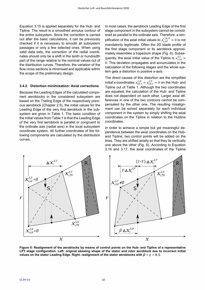
In most cases, the aeroblock Leading Edge of the first stage component in the subsystem cannot be consid-ered as parallel to the ordinate axis. Therefore, a sim-

plification of the axial initial values to R�,��,�/� # 0 is not

mandatorily legitimate. Often the 2D blade profile of the first stage component or its aeroblock approxi-mately resembles a trapezium shape (Fig. 6). Subse-

quently, the axial initial value of the Tipline is R�,��,� �0. This deviation propagates and accumulates in the calculation of the following stages and the whole sys-tem gets a distortion in positive x-axis.

The direct causes of this distortion are the simplified

initial x-coordinates R��,��,� # R��,��,� # 0 on the Hub- and

Tipline out of Table 1. Although the two coordinates are equated, the calculation of the Hub- and Tipline does not dependent on each other. Larger axial dif-ferences in one of the two contours cannot be com-pensated by the other one. The resulting misalign-ment can be solved separately for each individual component in the system by simply shifting the axial coordinates on the Tipline in relation to the Hubline coordinates.

In order to achieve a simple but yet meaningful de-pendence between the axial coordinates on the Hub- and Tipline, two control points will be added on the lines. They are shifted axially so that they lie vertically one above the other (Fig. 6). According to Equation 3.16 and 3.17, the axial coordinates of the Tipline

Figure 6: Realignment of the aeroblocks by means of control points on the Hub- and Tipline of a representative LPT stage configuration. Left: original skewing shape of the stator and rotor aeroblock due to incorrect initial

values on the stator Leading Edge. Right: realignment of the stator aeroblocks with � # � # �. �.

CC BY 4.0


10


(Leading and Trailing Edge) will be realigned within the considered component. The percentage position

of the control points on the line segment R[,��,�/�; R[,��,�/��

can be adjusted using the parameters and �.

3.16 R�,��,� # (R�,��,� E R�,�� ,�) ∙ ) ∆R� �,� ∙ � | , � ∈ G0,1H 3.17 R�,��,� # (R�,��,� E R�,�� ,�) ∙ E ∆R� �,� ∙ (1 ) �) | , � ∈ G0,1H The result of adjusting the Tipline with the control points on 50% of the length of the line segment is shown in Figure 6. The correction according to Equa-tion 3.16 varies the effective area, the shape and the position of the considered aeroblock in a minimal way.

An adjustment is usually only necessary for the very first component and can be applied directly after the calculation of this very first component aeroblock. All further sub-components use the coordinates of the Trailing Edge of the respective previously calculated sub-component aeroblock as initial values. Alterna-tively, the complete calculation of the axial (and ra-dial) coordinates of all partial components in the con-sidered subsystem can be run at first. Subsequently, the correction of the axial components must be ap-plied again to all previously calculated partial compo-nents. The result of both variants is approximately identical.

4. OUTLOOK

Based on the presented approaches of holistic 2D an-nulus contour design methods for axial aero tur-bomachinery systems, possible further developments and optimisation strategies can be defined.

Since each component in the subsystem is deter-mined by its own distribution curve, the number of stages in the considered subsystem significantly re-stricts the number of interpolation points per distribu-tion curve. Especially in the turbine configuration where often only a few stages are needed, certain in-accuracies in the calculated contour are possible. On the other hand, multi-stage systems such as the com-pressor, provide a sufficient number of support points and thus a stable and relatively smooth distribution curve. Therefore, a further consideration for smooth-ing the annulus contour by overlaying the calculated coordinates with a suitable spline function is possible.

In terms of Industry 4.0, the methods can be extended and superimposed by a combination of design and EHM databases (Engine Health Monitoring) as well as adaptive processes. In combination with various

design studies (DOE) a multitude of potential annulus structures can be found and evaluated. The results can be a gas path structure tailored to the specified application and needs of the customer.

In addition, complex optimisation processes can be set up for the targeted adaptation of the two-dimen-sional compressor and turbine annulus contours. In combination with pre-defined optimisation targets and design space parameters, the generically created gas path can serve as an initial geometry for complex aer-odynamic, thermodynamic and structural-mechanical optimisation processes. A smoothing and holistic op-timisation of the predetermined annulus structure would thus be possible.

5. CONCLUSION

In this paper a holistic approach for the preliminary design of 2D annulus contours for thermal axial tur-bomachinery systems is presented. The basis is a valid set of normalised distribution curves, which can be extracted from existing engines structures. The normalisation provides the possibility to perform a complete geometric pre-dimensioning of a turbine or compressor subsystem with the help of a few geomet-ric and topological input parameters. To correct pos-sible inaccuracies or contour distortions, several methods for axial and radial adjustment of the coordi-nates were given. The application and combination of one or more correction methods is optional and pro-vides a significant smoothing of the calculated con-tours with minimal influence on the axial and radial characteristics, the flow-conducting annulus structure and their cross sections. A direct integration of the re-sults as initial value for DOEs or more complex opti-misation processes is possible. The calculation ap-proaches presented in this paper offers a time-effi-cient and fully parametric possibility for the gas path pre-dimensioning for thermal turbo-machines.

ACKNOWLEDGEMENT

The work presented in this paper is part of the joint project VIT-V (Verfahren der Industrie 4.0 für die Triebwerks-Vorentwicklung; Methods of Industry 4.0 for the aircraft engine pre-development) founded through the ProFIT programme of the ILB (Investi-tionsbank des Landes Brandenburg) by EFRE (Eu-ropäische Fonds für regionale Entwicklung) , under

the contract No. 80173194.

Special thanks go to the project partner Rolls-Royce Deutschland Ltd. & Co KG without whom the project would not be possible.

CC BY 4.0


11


REFERENCES

[1] M. Hendler, S. Extra, M. Lockan, D. Bestle, P. Flassig, Compressor design in the context of holistic aero engine design, 18th AIAA/ISSMO Multidiscip. Anal. Optim. Conf. 2017. (2017) 1–9. https://doi.org/10.2514/6.2017-3334.

[2] S. Farokhi, Aircraft Propulsion, 2nd ed., John Wiley & Sons Ltd., 2014.

[3] W.J.G. Bräunling, Flugzeugtriebwerke: Grundlagen, Aero-Thermodynamik, ideale und reale Kreisprozesse, Thermische Turbomaschinen, Komponenten, Emissionen und Systeme, 4th ed., Springer Viehweg, Hamburg, 2015.

[4] R. Agromayor, L.O. Nord, Preliminary design and optimization of axial turbines accounting for diffuser performance, Int. J. Turbomachinery, Propuls. Power. 4 (2019). https://doi.org/10.3390/ijtpp4030032.

[5] A. Keskin, Process Integration and Automated Multi-Objective Optimization Supporting Aerodynamic Compressor Design, Brandenburgische Technische Universität Cottbus, 2007.

[6] L.F.Y. Sommer, Geometrieparametrisierungen für die aerodynamische Optimierung von Verdichterschaufelsektionen unter besonderer Berücksichtigung der Krümmung, Brandenburgische Technische Universität Cottbus, 2011.

[7] E. Lo Gatto, Y.G. Li, P. Pilidis, Gas turbine off-design performance adaptation using a genetic algorithm, in: Proc. ASME Turbo Expo, 2006: pp. 551–560. https://doi.org/10.1115/GT2006-90299.

[8] L. Moroz, C.R. Kuo, O. Guriev, Y.C. Li, B. Frolov, Axial turbine flow path design for an organic rankine cycle using R-245FA, Proc. ASME Turbo Expo. 5 A (2013) 1–8. https://doi.org/10.1115/GT2013-94078.

[9] M. Hendler, M. Lockan, D. Bestle, P. Flassig, Component-specific preliminary engine design taking into account holistic design aspects, Int. J. Turbomachinery, Propuls. Power. 3 (2018). https://doi.org/10.3390/ijtpp3020012.

[10] M. Hinz, Neue Parametrisierungsstrategien und Methoden der Prozessbeschleunigung für die Verdichteroptimierung, Shaker Verlag (Aachen), 2012.

[11] W. Traupel, Neue Allgemeine Theorie der Mehrstufigen Axialen Turbomaschine, (1942).

[12] P. De haller, Das Verhalten von Tragflügelgittern in Axialverdichtern und im Windkanal, Brennstoff-Wärme-Kraft. 5 (1953) 333–337.

[13] A.D.S. Carter, S.J. Andrews, E.A. Fielder, The Design and Testing of an Axial Compressor having a Mean Stage Temperature Rise of 3 ° deg C, Aeronaut. Res. Counc. Reports Memo. 2985 (1957).

[14] F. Torniello, G. Mardersteig, B. Radice, O. Bodoni, The Alphabet of Francesco Torniello da Novara: Followed by a Comparison with the Alphabet of Fra Luca Pacioli, Montagnola di Lugano, 1517.

[15] P.C. Sikkema, Über den Grad der Approximation mit Bernstein-Polynomen, Numer. Math. 1 (1959) 221–239. https://doi.org/10.1007/BF01386387.

[16] A. Müller, Neuere Gedanken des Monsieur Paul de Faget de Casteljau, Technische Universität Braunschweig, 1995.

[17] J. Hoschek, D. Lasser, Grundlagen der geometrischen Datenverarbeitung, B. G. Teubner Stuttgart, 1992. https://doi.org/10.1007/978-3-322-89829-6.

CC BY 4.0


12


Documents

A Holistic Approach for the Generic Preliminary Design of