A Hierarchy of Models for Microgrids WithGrid-Feeding Inverters

Olaolu Ajala∗, Murilo Almeida†, Ivan Celanovic†, Peter Sauer∗, and Alejandro Domınguez-Garcıa∗∗Department of Electrical and Computer Engineering

University of Illinois at Urbana Champaign306 N Wright St, Urbana, IL 61801 USA

Email: ooajala2, psauer, aledan@illinois.edu†Typhoon HIL, Inc., 35 Medford St. Suite 305, Somerville, MA 02143

Email: murilo.almeida, ivanc@typhoon-hil.com

Abstract—This work develops a hierarchy of models,each with distinct time resolutions, for microgrids havinggrid-feeding inverters at all generation buses. Specifically,our focus is on microgrids with battery storage unitsconnected to an electrical network via grid-feeding in-verters. The process of developing the model hierarchyinvolves three key stages: (1) the formulation of a microgridhigh-order model using circuit-theoretic and control laws,(2) the systematic reduction of this high-order model todistinct reduced-order models using singular perturbationtechniques, and (3) an identification of the time resolutionsfor which each reduced-order model is valid. A comparisonbetween the responses of all the models developed and thatof a microgrid ultra-high fidelity model is presented.

I. INTRODUCTION

A microgrid may be defined as a collection of loadsand distributed energy resources (DERs), interconnectedvia an electrical network with a small physical footprint,which is capable of operating in (1) grid-connectedmode, as part of a large power system; or (2) islandedmode, as an autonomous power system. The DERs thatconstitute a microgrid are often interfaced to the elec-trical network via a grid-feeding inverter, where the realand reactive power injections are controlled to track agiven reference; or via a grid-forming inverter, where theoutput voltage magnitude and frequency are controlledto track a given reference.

As the popularity and adoption of the microgridconcept in electricity systems increases, it becomesnecessary to develop comprehensive mathematical mod-els. Models are tools that control engineers, scientists,mathematicians, and other non experts in the field of

∗The information, data, or work presented herein was supportedby the Advanced Research Projects Agency-Energy (ARPA-E), U.S.Department of Energy, within the NODES program, under Award DE-AR0000695.

microgrids, require for the different analysis and controldesign tasks necessary for development of innovativemicrogrid technologies. Accurate mathematical modelsmay be developed for inverter-based microgrids by uti-lizing concepts from circuit-theoretic and control theory.However, the resulting models are often highly complexand too detailed for the particular application. It thereforebecomes necessary to simplify these models to lessdetailed ones which, though less accurate, can representthe phenomena relevant to the application of interest.

The main contribution of this paper is the develop-ment of a time-resolution-based hierarchy of models forinverter-based microgrids, and an identification of thetime resolution for which each model is valid. The focusof this work is on microgrids with power supplies con-nected to an electrical network via grid-feeding inverters.Using Kirchhoff’s laws, component terminal relations,and basic control law definitions, a microgrid high-ordermodel (µHOm) is developed. Afterwards, two reduced-order models, referred to as microgrid reduced-ordermodel 1 (µROm1) and microgrid reduced-order model 2(µROm2), are obtained from the µHOm using singularperturbation techniques for model-order reduction. Thetime resolution for which the reduced-order models arevalid is identified, and all three models are explicitlypresented with the small parameters used for singularperturbation analysis identified. Finally, for some testcases, the responses of all three models are comparedto that of a microgrid ultra-high fidelity model (UHΦm)that is: (1) designed to mimic a real system, and (2) mod-eled on a real-time simulator platform developed byTyphoon HIL, Inc. [1].

The development of mathematical models for micro-grids with grid-feeding inverters has received significant

attention in the research community. Recent work inthis area includes formulations of (1) switched models,referred to as the UHΦm in this work, which are verydetailed and capture the high frequency switching tran-sients introduced by the inverter Pulse Width Modulation(PWM) mechanism [15], (2) averaged models, referredto as the µHOm in this work, which are slightly lesselaborate and describe dynamics of the average values ofvariables, neglecting the PWM switching transients [15],and (3) reduced-order models, referred to as µROm2in this paper, which approximate the inverter-interfacedpower supply with a constant power source. Althoughthe formulations of these models are usually detailed,authors fail to identify the time resolutions associatedwith the different models. More specifically, Pogakuet al. [11] presents a high-order model for grid-forming-inverter based microgrids but exclude a discussion onmodel-order reduction. Anand and Fernandes [3], andRasheduzzaman et al. [12] present reduced-order modelsfor microgrids but the models are obtained using small-signal analysis, which is only valid within certain oper-ating regions. Kodra et al. [7] discuss the model-orderreduction of an islanded microgrid using singular pertur-bation analysis. However, the electrical network dynam-ics are not included in the high-order model presented,and a simple linear model, which does not fully capturethe dynamics of the islanded microgrid, is used for thesingular perturbation analysis. Schiffer et al. [14] developa detailed high-order model for grid-feeding-inverter-based microgrids, and singular perturbation analysis isemployed to perform time-scale separation and model-order reduction with the underlying assumptions stated.However, though the authors claim that the model-orderreduction can be performed, the small parameters in themodel used for singular perturbation analysis are not ex-plicitly identified, and details of the singular perturbationanalysis are not presented. Also, just one reduced-ordermodel is developed, and the time resolution associatedwith the model is not identified.

II. PRELIMINARIES

In this section, we first introduce the qd0 transfor-mation of three-phase variables to arbitrary and syn-chronous reference frames. Next, we introduce graph-theoretic notions used in later developments to developthe microgrid network model. Finally, a primer on sin-gular perturbation analysis for model-order reduction ispresented.

A. The qd0 Transformation

Let α(t) denote the angular position of a referenceframe rotating at an arbitrary angular velocity, ω(t), andlet fqd0[α(t)](t) =

[fq[α(t)](t) fd[α(t)](t) f0[α(t)](t)

]Tdenote the qd0 transform of a vector of 3-phase vari-ables, fabc(t) =

[fa(t) fb(t) fc(t)

]T, to the reference

frame. The general form of the non-power-invariant qd0transformation is given by:

fqd0[α(t)](t) = K1(α(t))fabc(t), (1)

where:

K1(α(t)) =2

3

cos(α(t)) cos(α(t)− 2π3 ) cos(α(t) + 2π

3 )sin(α(t)) sin(α(t)− 2π

3 ) sin(α(t) + 2π3 )

12

12

12

,α(t) =

∫ t

0

ω(τ) dτ + α(0).

The qd0 reference frame in (1) is referred to as thearbitrary reference frame, but when α(t) = ω0t, whereω0 denotes the synchronous frequency, it is referred toas the synchronously rotating reference frame [9].

Assume that fa(t), fb(t), and fc(t) are a balancedthree-phase set. Let

−→f qd0[ω0t](t) and

−→f qd0[α(t)](t) de-

note the complex representation of fabc(t) in the syn-chronously rotating reference frame and the arbitraryreference frame, respectively. Then, by using (1), wehave that for

−→f qd0[·](t) := fq[·](t)− jfd[·](t), (2)

where j denotes the complex variable, i.e., j =√−1,

−→f qd0[α(t)](t) =

−→f qd0[ω0t](t) exp(−jδ(t)), (3)

with

δ(t) := α(t)− ω0t.

[Note that because of the balanced assumption on fa(t),fb(t), and fc(t), f0[α(t)](t) = 0.]

Let fqd0[α(t)](t) =[fq[α(t)](t) fd[α(t)](t)

]T, and

fqd0[ω0t](t) =[fq[ω0t](t) fd[ω0t](t)

]T; then from (2)–

(3), it follows that:

fqd0[α(t)](t) = K2(δ(t))fqd0[ω0t](t), (4)

with

K2(δ(t)) =

[cos(δ(t)) − sin(δ(t))sin(δ(t)) cos(δ(t))

],

and the evolution of δ(t) governed by:

dδ(t)

dt= ω(t)− ω0. (5)

2

B. Graph-Theoretic Network Model

The topology of the microgrid electrical network canbe described by a connected undirected graph, G =(V, E), with V denoting the set of buses in the network,so that V := 1, 2, . . . , |V|, and E ⊂ V × V ,so that j, k ∈ E if buses j and k are electricallyconnected. Choose an arbitrary orientation for each ofthe elements in E ; then we can define an incidencematrix, M = [mie] ∈ Rn×|E|, associated with thisorientation as follows:

mie = 1 if edge e is directed away from node i,mie = −1 if edge e is directed into node i,mie = 0 if edge e is not incident on node i.

Connected to some buses, we assume that there is aninverter-interfaced source, the dynamics of which aredescribed in Section III-A; and at each bus, we assumethere is another element, the dynamics of which aredescribed by a generic dynamical model satisfying someproperties, as described in Section III-C.

Let VI ⊆ V denote the set of buses with an inverter-interfaced source. For j = 1, 2, . . . ,|VI |, let sj be used toidentify variables associated with the inverter-interfacedsource connected to bus j. As a result, we can representthe resistance, inductance and current injection of thesource as: R(sj), L(sj) and I(sj)(t), respectively.

For j = 1, 2, . . . ,|V|, let lj be used to identifyvariables associated with an element connected to bus j.As a result, we can represent the resistance, inductanceand current injection of the element as: R(lj), L(lj) andI(lj)(t), respectively.

For m = 1, 2, . . . ,|E|, let em := j, k, j, k ∈ E .As a result, we can represent the resistance, inductanceand current across a line extending from bus j to bus kas: R(em), L(em) and I(em)(t), respectively.

C. A Primer on Singular Perturbation Analysis

Definition (Big O notation). Consider a function f(ε),defined on some subset of the real numbers. We writef(ε) = O

(εk)

if and only if there exists a positive realnumber C, such that:∣∣f(x)

∣∣ ≤ Cεk, as ε→ 0.

The material in this section follows closely from thedevelopments in ([8], pp. 1–12) and ([6], pp. 7–11).Consider the following two-time-scale dynamical model:

x(t) = f(x(t), z(t),w(t), ε

), x(0) = x0,

εz(t) = g(x(t), z(t),w(t), ε

), z(0) = z0,

0 = h(x(t), z(t),w(t), ε

), w(0) = w0,

(6)

with slow and fast time-scales, t and τ = tε , re-

spectively, where f (·, ·, ·, ε) = O(1), g (·, ·, ·, ε) =O(1), and h (·, ·, ·, ε) = O(1).

Assumption II.1. Let the bar (¯) and tilde (˜) notationsbe used to describe the slow t-scale and fast τ -scalevariables, respectively. x, z and w can be decoupled to

x(t) = x(t) + x(τ),

z(t) = z(t) + z(τ),

w(t) = w(t) + w(τ),

where

x(t) = x0(t) + εx1(t) + ε2x2(t) + · · · ,x(τ) = x0(τ) + εx1(τ) + ε2x2(τ) + · · · ,z(t) = z0(t) + εz1(t) + ε2z2(t) + · · · ,z(τ) = z0(τ) + εz1(τ) + ε2z2(τ) + · · · ,w(t) = w0(t) + εw1(t) + ε2w2(t) + · · · ,w(τ) = w0(τ) + εw1(τ) + ε2w2(τ) + · · · .

The dynamical model in (6) may be rewritten in termsof t and τ as:

˙x(t) +1

ε

dx(τ)

dτ= f

(x(t) + x(τ), z(t) + z(τ), w(t) + w(τ), ε

),

ε ˙z(t) +dz(τ)

dτ= g

(x(t) + x(τ), z(t) + z(τ), w(t) + w(τ), ε

),

0 = h(x(t) + x(τ), z(t) + z(τ), w(t) + w(τ), ε

),

and by setting ε = 0, it follows that:

dx0(τ)

dτ= 0,

˙x0(t) = f(x0(t) + x0(∞), z0(t) + z0(∞), w0(t) + w0(∞), 0

),

dz0(τ)

dτ= g

(x0(0) + x0(τ), z0(0) + z0(τ), w0(0) + w0(τ), 0

),

and

0 = h(x0(0) + x0(τ), z0(0) + z0(τ), w0(0) + w0(τ), 0

),

0 = h(x0(t) + x0(∞), z0(t) + z0(∞), w0(t) + w0(∞), 0

).

(7)

Assumption II.2. Equation (7) has distinct real roots,one of which is:

w0(0) + w0(τ) = ν(x0(0) + x0(τ), z0(0) + z0(τ)

),

w0(t) + w0(∞) = ν(x0(t) + x0(∞), z0(t) + z0(∞)

).

Choosing initial conditions x0(0) = 0 and x0(0) =x0, let z0(t) = ζ

(x0(t)

)be a root of

0 = g(x0(t), z0(t), ν

(x0(t), z0(t)

), 0). (8)

As a result, the two-time-scale dynamical model in (6)may be expressed in the approximate form:

˙x0(t) = f(x0(t), ζ(x0(t)), ν

(x0(t), ζ(x0(t))

), 0),

(9)

3

anddz0(τ)

dτ= g

(x0, ζ(x0) + z0(τ), ν(x0, ζ(x0) + z0(τ)), 0

),

(10)where x0(0) = x0 and z0(0) = z0 − ζ(x0)

Assumption II.3. The equilibrium z0(τ) = 0 of (10)is asymptotically stable in x0, and z0(0) belongs to itsdomain of attraction.

Assumption II.4. The eigenvalues of ∂g∂z , the Jacobian

of (8), evaluated, for ε = 0, along x0(t), z0(t), havereal parts smaller than a fixed negative number.

Theorem (Tikhonov’s theorem). Let f and g in (6)be sufficiently many times continuously differentiablefunctions of their arguments, and let the root, z0(t) =ζ(x0(t)

)of (8) be distinct and real, in the domain of

interest. Then, if assumptions II.1, II.2, II.3 and II.4 aresatisfied, (6) can be approximated by (9) and (10), where

x(t) = x0(t) +O(ε),

z(t) = ζ(x0(t)) + z0(τ) +O(ε),

w(t) = ν(x0(t), ζ(x0(t)) + z0(τ)

)+O(ε),

and there exists t0 > 0 such that

z(t) = ζ(x0(t)) +O(ε),

w(t) = ν(x0(t), ζ(x0(t))

)+O(ε),

for all t > t0.

In this work, we refer to

˙x0(t) = f(x0(t), ζ(x0(t)), ν

(x0(t), ζ(x0(t))

), 0)(11)

as the reduced-order model i.e. the approximateslow component.

Definition (Time resolution). The time-resolution of thereduced-order in (11) is the time t0 such that z0(τ) = 0,for all t > t0.

Consider the dynamical model in (6). If we choose εsuch that − 1

ε is greater than the real part of eigenvaluesassociated with the fast dynamics, then the fast modelin (10) reaches equilibrium z0(τ) = 0 in around 5εseconds. As a result, we say that the time resolutionof the reduced-order model in (11) is 5ε seconds.

III. MICROGRID HIGH-ORDER MODEL

In this section, basic circuit laws are used in con-junction with notions introduced in Section II to de-velop a High-Order model for a grid-feeding-inverter-based AC microgrid operating in grid-connected mode.

First, a model is developed for an inverter-interfacedsource, which includes a battery, a 3-phase inverter, anLCL filter, an outer power controller and inner currentcontroller, and a phase-locked loop. Next, a three-phasemodel for the electrical network is developed, alongwith a generic model for an element (typically a load)connected between each bus and the ground.

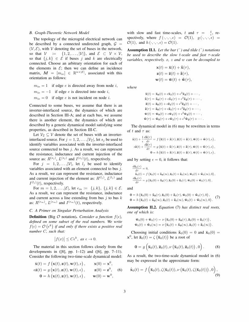
The Microgrid High-Order Model (µHOm), whosesystem model is depicted in Fig. 1 below, is developed bycombining the inverter-interfaced source model, the net-work model and the generic element model. In this work,the models developed are expressed using the per-unitrepresentation, to ease analysis in later developments.

POWER CONTROLLER

PHASE-LOCKED LOOP

BATTERYTHREE-PHASE

INVERTERTHREE-PHASE

INVERTER

LCL FILTER

LCL FILTER

NetworkNetworkjjbus

POWER CONTROLLER

PHASE-LOCKED LOOP

BATTERYTHREE-PHASE

INVERTER

LCL FILTER

Networkjbus

THREE-PHASE LOAD

kkbus

Fig. 1: Microgrid Model.

A. Inverter-Interfaced Source Model

The structure of the inverter-interfaced source adoptedin this work, shown in Fig. 1, is comprised of a 3-phase inverter coupled with a battery, an LCL filter,a power controller and a phase-locked loop (PLL). Anaveraged model, as opposed to a switched model, is usedto describe the 3-phase inverter dynamics (see [15], pp.27–38, for more details).

For the inverter connected to bus j of the microgridnetwork, let V (sj)

DC denote the dc voltage at the inverterinput. Let U (sj)(t), E(sj)(t), E(sj)(t) and V (sj)(t) de-note the Pulse Width Modulation (PWM) output voltageof the inverter, the internal voltage of the inverter, theLCL filter capacitor voltage, and the voltage at busj, in per-unit representation, respectively. Let Ξ(sj)(t)and I(sj)(t) denote the inverter output current and thefiltered inverter output current, in per-unit representation,respectively. Let Γ(sj)(t) denote the state variable forthe current controller, in per-unit representation. Let

4

P (sj)r and Q(sj)

r denote the inverter three-phase realand reactive power references, in per-unit representation,respectively. Let Λ(sj)(t) denote the state variable forthe phase-locked loop (PLL), in per-unit representation.Then, using the qd0 transformation discussed in Sec-tion II, the dynamics of the inverter-interfaced sourceconnected to bus j of the microgrid electrical networkcan be described by:

1

ω0

dδ(sj)(t)

dt=−K(sj)

Pλ E(sj)

d[α(j)(t)](t) +K

(sj)

Iλ Λ(sj)

[α(j)(t)](t)− 1,

L(sj)

ω0

dI(sj)

q[ω0t](t)

dt=−R(sj)I

(sj)

q[ω0t](t)− L(sj)I

(sj)

d[ω0t](t) + E

(sj)

q[ω0t](t)

− V (lj)

q[ω0t](t),

L(sj)

ω0

dI(sj)

d[ω0t](t)

dt= L(sj)I

(sj)

q[ω0t](t)−R(sj)I

(sj)

d[ω0t](t) + E

(sj)

d[ω0t](t)

− V (lj)

d[ω0t](t),

C(sj)

ω0

dE(sj)

q[ω0t](t)

dt=− I(sj)q[ω0t]

(t)− C(sj)E(sj)

d[ω0t](t) + Ξ

(sj)

q[ω0t](t),

C(sj)

ω0

dE(sj)

d[ω0t](t)

dt=− I(sj)d[ω0t]

(t) + C(sj)E(sj)

q[ω0t](t) + Ξ

(sj)

d[ω0t](t),

L(sj)

0

ω0

dΞ(sj)

q[α(j)(t)](t)

dt=V

(sj)

DC K(sj)

Iγ

2Γ(sj)

q[α(j)(t)](t)

−

R(sj)

0 +V

(sj)

DC K(sj)

Pγ

2

Ξ(sj)

q[α(j)(t)](t)

+V

(sj)

DC K(sj)

Pγ

2

P(sj)r E

(sj)

q[α(j)(t)](t)−Q

(sj)r E

(sj)

d[α(j)(t)](t)

E(sj)

q[α(j)(t)](t)2 + E

(sj)

d[α(j)(t)](t)2

,

L(sj)

0

ω0

dΞ(sj)

d[α(j)(t)](t)

dt=V

(sj)

DC K(sj)

Iγ

2Γ(sj)

d[α(j)(t)](t)

−

R(sj)

0 +V

(sj)

DC K(sj)

Pγ

2

Ξ(sj)

d[α(j)(t)](t)

+V

(sj)

DC K(sj)

Pγ

2

P(sj)r E

(sj)

d[α(j)(t)](t) + Q

(sj)r E

(sj)

q[α(j)(t)](t)

E(sj)

q[α(j)(t)](t)2 + E

(sj)

d[α(j)(t)](t)2

,

E(sj)

q[α(j)(t)](t) =

(−I(sj)

q[α(j)(t)](t) + Ξ

(sj)

q[α(j)(t)](t))R

(sj)

0

+ E(sj)

q[α(j)(t)](t),

E(sj)

d[α(j)(t)](t) =

(−I(sj)

d[α(j)(t)](t) + Ξ

(sj)

d[α(j)(t)](t))R

(sj)

0

+ E(sj)

d[α(j)(t)](t),

Eqd0[α(j)(t)](t) = K2(δ(sj)(t))Eqd0[ω0t](t),

Ξqd0[α(j)(t)](t) = K2(δ(sj)(t))Ξqd0[ω0t](t),

1

ω0

dΓ(sj)

q[α(j)(t)](t)

dt=

P(sj)r E

(sj)

q[α(j)(t)](t)−Q

(sj)r E

(sj)

d[α(j)(t)](t)

E(sj)

q[α(j)(t)](t)2 + E

(sj)

d[α(j)(t)](t)2

− Ξ(sj)

q[α(j)(t)](t),

1

ω0

dΓ(sj)

d[α(j)(t)](t)

dt=

P(sj)r E

(sj)

d[α(j)(t)](t) + Q

(sj)r E

(sj)

q[α(j)(t)](t)

E(sj)

q[α(j)(t)](t)2 + E

(sj)

d[α(j)(t)](t)2

− Ξ(sj)

d[α(j)(t)](t),

1

ω0

dΛ(sj)

[α(j)(t)](t)

dt=− E(sj)

d[α(j)(t)](t).

(12)

where L(sj)0 , L(sj) and C(sj) denote the inductances and

capacitance of the LCL filter, in per-unit representation,respectively; R(sj)

0 , R(sj)0 and R(sj) denote the inverter

and filter resistances, in per-unit representation, respec-

tively; K(sj)Pγ and K

(sj)Iγ denote the proportional and

integral control gains for the current controller, in per-unit representation, respectively; K(sj)

Pλ and K(sj)Iλ denote

the proportional and integral controller gains for thePLL, in per-unit representation, respectively. Filtered realand reactive power measurements, P (sj)

f (t) and Q(sj)f (t),

can be described by:

1

ω(sj)c

dP(sj)f (t)

dt=− P (sj)

f (t) + E(sj)

q[ω0t](t)I

(sj)

q[ω0t](t) + E

(sj)

d[ω0t](t)I

(sj)

d[ω0t](t),

1

ω(sj)c

dQ(sj)f (t)

dt=−Q(sj)

f (t) + E(sj)

q[ω0t](t)I

(sj)

d[ω0t](t)− E(sj)

d[ω0t](t)I

(sj)

q[ω0t](t),

with ω(sj)c denoting the filter cut-off frequency.

B. Network Model

Assumption III.1. All lines connecting the networkbuses can be represented using the short transmissionline model [5].

Let V (lj)

q[ω0t](t)− jV

(lj)

d[ω0t](t) denote the per-unit voltage

at bus j, and let R(em), L(em) and I(em)q[ω0t]

(t)− jI(em)d[ω0t]

(t)denote the per-unit resistance, inductance and currentacross line (j, k), respectively, as introduced in Sec-tion II-B. Then, the voltage across a line connecting busj and bus k of the network can be described by:

V(lj)

q[ω0t](t)− V (lk)

q[ω0t](t) =

L(em)

ω0

dI(em)q[ω0t]

(t)

dt+R(em)I

(em)q[ω0t]

(t) + L(em)I(em)d[ω0t]

(t),

V(lj)

d[ω0t](t)− V (lk)

d[ω0t](t) =

L(em)

ω0

dI(em)d[ω0t]

(t)

dt+R(em)I

(em)d[ω0t]

(t)− L(em)I(em)q[ω0t]

(t).

Let

V(V)q[ω0t]

(t) =[V

(l1)q[ω0t]

(t) V(l2)q[ω0t]

(t) · · · V(l|V|)

q[ω0t](t)]T,

V(V)d[ω0t]

(t) =[V

(l1)d[ω0t]

(t) V(l2)d[ω0t]

(t) · · · V(l|V|)

d[ω0t](t)]T,

I(E)q[ω0t]

(t) =[I(e1)q[ω0t]

(t) I(e2)q[ω0t]

(t) · · · I(e|E|)

q[ω0t](t)]T,

I(E)d[ω0t]

(t) =[I(e1)d[ω0t]

(t) I(e2)d[ω0t]

(t) · · · I(e|E|)

d[ω0t](t)]T.

Then the network dynamics are described by:

1

ω0L(E)

dI(E)q[ω0t]

(t)

dt=−R(E)I

(E)q[ω0t]

(t)− L(E)I(E)d[ω0t]

(t)

+ MTV(V)q[ω0t]

(t),

1

ω0L(E)

dI(E)d[ω0t]

(t)

dt=−R(E)I

(E)d[ω0t]

(t) + L(E)I(E)q[ω0t]

(t)

+ MTV(V)d[ω0t]

(t).

(13)

with

R(E) = diag(R(e1), R(e2), · · · , R(e|E|)

),

L(E) = diag(L(e1), L(e2), · · · , L(e|E|)

),

5

where diag(d(1), d(2), · · · , d(n)

)is a diagonal

matrix with diagonal entries d(1), d(2), . . . , d(n); andM denotes the network incidence matrix as defined inSection II.

C. Generic Element Model

Let V (lj)

q[ω0t](t)− jV

(lj)

d[ω0t](t) denote the per-unit voltage

at bus j, and let I(lj)q[ω0t](t) − jI

(lj)

d[ω0t](t) denote the per-

unit current injection by an element (typically a load) atbus j. The dynamics can be described by a generic non-linear system of differential equations which we assumeto be of the form:

µ(lj)V V

(lj)

q[ω0t](t) = qV

(V

(lj)

q[ω0t](t), V

(lj)

d[ω0t](t), I

(lj)

q[ω0t](t), I

(lj)

d[ω0t](t)),

µ(lj)V V

(lj)

d[ω0t](t) = dV

(V

(lj)

q[ω0t](t), V

(lj)

d[ω0t](t), I

(lj)

q[ω0t](t), I

(lj)

d[ω0t](t)),

µ(lj)I I

(lj)

q[ω0t](t) = qI

(V

(lj)

q[ω0t](t), V

(lj)

d[ω0t](t), I

(lj)

q[ω0t](t), I

(lj)

d[ω0t](t)),

µ(lj)I I

(lj)

d[ω0t](t) = dI

(V

(lj)

q[ω0t](t), V

(lj)

d[ω0t](t), I

(lj)

q[ω0t](t), I

(lj)

d[ω0t](t)),

(14)

where µ(lj)V and µ

(lj)I represent time constants of the

generic element at bus j; and qV(·, ·, ·, ·

), dV

(·, ·, ·, ·

),

qI(·, ·, ·, ·

), and dI

(·, ·, ·, ·

)are nonlinear functions of its

state variables.

IV. MICROGRID REDUCED-ORDER MODEL 1

Using the singular perturbation techniques discussedin Section II-C, we reduce the order (state-space dimen-sion) of the µHOm described in (12)–(14) to obtain theµROm1.

Assumption IV.1. For ε1 = 1 × 10−3, there ex-ists k

(j)i , k(m) ∈ (0, 10), i = 1, 2, . . . , such

that: C(sj)

ω0= k

(j)1 ε1,

L(sj)

ω0= k

(j)2 ε1,

L(sj)

0ω0

=

k(j)3 ε1, µ

(lj)

V = k(j)4 ε1, µ

(lj)

I = k(j)5 ε1,

1ω0

= k(j)6 ε1,

1ω0

L(E) = diag(k(1), k(2), · · · , k(|E|)

)ε1.

Assumption IV.2. The dynamic properties of the µHOmare such that: at each bus j, for

x1(t) =

[P

(sj)

f (t) Q(sj)

f (t) Γ(sj)

q[α(j)(t)](t) Γ

(sj)

d[α(j)(t)](t)

]T,

z1(t) =

[δ(sj)(t) I

(sj)

q[ω0t](t) I

(sj)

d[ω0t](t) Λ

(sj)

[α(j)(t)](t)

E(sj)

q[ω0t](t) E

(sj)

d[ω0t](t) Ξ

(sj)

q[α(j)(t)](t)

Ξ(sj)

d[α(j)(t)](t) I

(lj)

q[ω0t](t) I

(lj)

d[ω0t](t)

V(lj)

q[ω0t](t) V

(lj)

d[ω0t](t) I

(E)q[ω0t]

(t) I(E)d[ω0t]

(t)]T,

w1(t) =[E

(sj)

q[ω0t](t) E

(sj)

d[ω0t](t)]T, the dynamics of z1(t)

are faster than those of x1(t), and the µHOm can beexpressed compactly as follows:

x1(t) = f1(x1(t), z1(t),w1(t), ε1

),

ε1z1(t) = g1(x1(t), z1(t),w1(t), ε1

),

0 = h1(x1(t), z1(t),w1(t), ε1

).

(15)

Assumption IV.3. Equation (15) satisfies the conditionsfor Tikhonov’s theorem, as presented in Section II-C.

Given Assumptions IV.1–IV.3, the µHOm can bereduced to the model,

˙x0[1](t) = f1

(x0[1](t), ζ1(x0[1](t)), ν1

(x0[1](t), ζ1(x0[1](t))

), 0

),

which is the so-called Microgrid Reduced-OrderModel 1 (µROm1). The explicit ordinary differ-ential equations (ODEs) that constitute µROm1are derived in Appendix B

V. MICROGRID REDUCED-ORDER MODEL 2Using the singular perturbation techniques discussed

in Section II-C, we reduce the order (state-space dimen-sion) of the µHOm to obtain the µROm2.

Assumption V.1. For ε2 = 1 × 10−1, there ex-ists k

(j)i , k(m) ∈ (0, 10), i = 1, 2, . . . , such

that: C(sj)

ω0= k

(j)1 ε2,

L(sj)

ω0= k

(j)2 ε2,

L(sj)

0ω0

=

k(j)3 ε2, µ

(lj)

V = k(j)4 ε2, µ

(lj)

I = k(j)5 ε2,

1ω0

= k(j)6 ε2,

1ω0

L(E) = diag(k(1), k(2), · · · , k(|E|)

)ε2,

2R(sj)

0 +V(sj)

DC K(sj)

Pγ

ω0V(sj)

DC K(sj)

Iγ

= k(j)5 ε2.

Assumption V.2. The dynamic properties of the µHOmare such that: at each bus j, forx2(t) =

[P

(sj)

f (t) Q(sj)

f (t)]T,

z2(t) =

[Γ(sj)

q[α(j)(t)](t) Γ

(sj)

d[α(j)(t)](t) I

(sj)

q[ω0t](t)

I(sj)

d[ω0t](t) E

(sj)

q[ω0t](t) E

(sj)

d[ω0t](t) Ξ

(sj)

q[α(sj)(t)]

(t)

Ξ(sj)

d[α(j)(t)](t) Λ

(sj)

[α(j)(t)](t) I

(lj)

q[ω0t](t) I

(lj)

d[ω0t](t)

V(lj)

q[ω0t](t) V

(lj)

d[ω0t](t) I

(E)q[ω0t]

(t) I(E)d[ω0t]

(t) δ(sj)(t)]T,

w2(t) =[E

(sj)

q[ω0t](t) E

(sj)

d[ω0t](t)]T, the dynamics of z2(t)

are faster than those of x2(t), and the µHOm can beexpressed compactly as follows:

x2(t) = f2(x2(t), z2(t),w2(t), ε2

),

ε2z2(t) = g2(x2(t), z2(t),w2(t), ε2

),

0 = h2(x2(t), z2(t),w2(t), ε2

).

(16)

Assumption V.3. Equation (16) satisfies the conditionsfor Tikhonov’s theorem, as presented in Section II-C.

6

Given Assumptions V.1–V.3, the µHOm can bereduced to the model,

˙x0[2](t) = f2

(x0[2](t), ζ2(x0[2](t)), ν2

(x0[2](t), ζ2(x0[2](t))

), 0

),

which is the so-called Microgrid Reduced-OrderModel 2 (µROm2). The explicit ODEs that con-stitute µROm2 are derived in Appendix C

VI. COMPARISON OF UHΦM, µHOM, µROM1 ANDµROM2

In this section, the time resolution of each reduced-order model is discussed, and for given test cases, theresponses of UHΦm, µHOm, µROm1 and µROm2 arecompared and validated.

A. Reduced-Model Time Resolution

For formulation of µROmi, where i = 1, 2, εi waschosen such that 1

10εirepresents the largest eigenvalues

of the system, associated with the fast states zi(t). Con-sequently, the fast-varying terms in the system responsereach steady state in approximately 50εi seconds and thetime resolution of µROmi is 50εi seconds. Table I showsthe time resolution for the reduced-order models.

TABLE I: Reduced-Model Time Resolution

small parameter time-resolutionµROm1 ε1 = 1× 10−3 50 msµROm2 ε2 = 0.1 5 s

B. Model Validation

To validate the µHOm, µROm1 and µROm2, thefollowing test case is employed: a grid-feeding inverterconnected to an infinite bus through a short transmissionline. Using the µHOm, µROm1 and µROm2 respec-tively, we developed the test case in Simulink. We alsodesigned an ultra-high fidelity model (UHΦm) of thetest case on a real-time simulator device called theHIL 402, which was developed by Typhoon HIL [1]. Theproperties of UHΦm and µHOm are shown in Table IIbelow.

Firstly, we use a step response analysis to compare theUHΦm, µHOm, µROm1 and µROm2. The simulationstarts at t = 0, and the system is in steady state withthe power references taking values P (s1)

r = 12kW andQ(s1)r = 9kW. At t = 0.1s, the real power reference

TABLE II: UHΦm vs µHOm

Parameters UHΦm µHOm

LCL Filter

r(s1)0 0.1Ω 0.1Ω

l(s1)0 3mH 3mHr(s1) 1mΩ 1mΩ

l(s1) 2µH 2µHr(s1)0 15mΩ 15mΩ

c(s1) 20µF 20µF

PWM Inverter Model Switched AveragedRating 35kW 35kW

Current Controller Gains Proportional 0.015 0.015Integral 1 1

PLL Filter? Yes NoProportional 100 100

Integral 3200 3200Derivative 1 0

Network r(e1) 8mΩ 8mΩ

l(e1) 3µH 3µH

∞ Bus Voltage Magnitude 227V 227VAngle 0 0

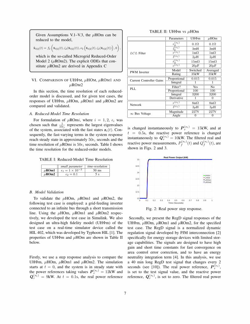
is changed instantaneously to P (s1)r = 15kW, and at

t = 0.5s, the reactive power reference is changedinstantaneously to Q(s1)

r = 10kW. The filtered real andreactive power measurements, P (s1)

f (t) and Q(s1)f (t), are

shown in Figs. 2 and 3.

0 0.1 0.2 0.3 0.4 0.5 0.6 0.7 0.8 0.9 1Time (Seconds)

12

12.5

13

13.5

14

14.5

15

Real Power Output (kW)

UHΦmµHOmµROm1µROm2

Fig. 2: Real power step response.

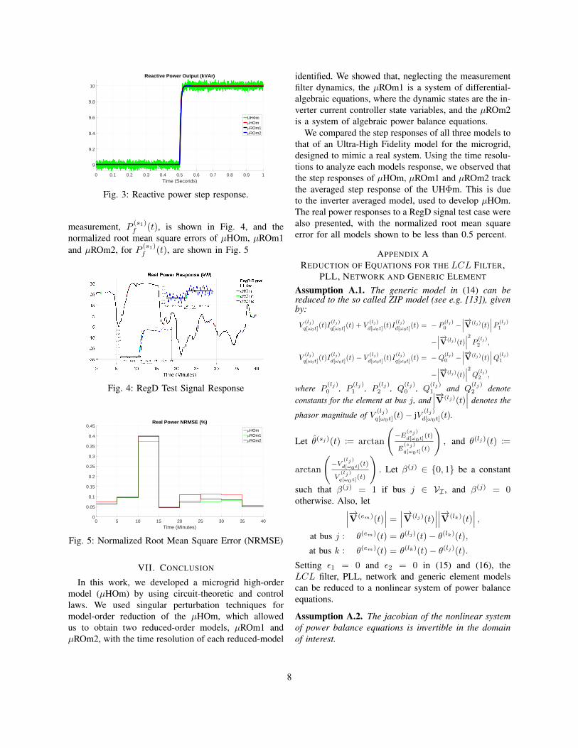
Secondly, we present the RegD signal responses of theUHΦm, µHOm, µROm1 and µROm2, for the specifiedtest case. The RegD signal is a normalized dynamicregulation signal developed by PJM interconnection [2]specifically for energy storage devices with limited stor-age capabilities. The signals are designed to have highgain and short time constants for fast convergence onarea control error correction, and to have an energyneutrality integration term [4]. In this analysis, we usea 40 min long RegD test signal that changes every 2seconds (see [10]). The real power reference, P (s1)

r ,is set to the test signal value, and the reactive powerreference, Q(s1)

r , is set to zero. The filtered real power

7

0 0.1 0.2 0.3 0.4 0.5 0.6 0.7 0.8 0.9 1Time (Seconds)

9

9.2

9.4

9.6

9.8

10

Reactive Power Output (kVAr)

UHΦmµHOmµROm1µROm2

Fig. 3: Reactive power step response.

measurement, P (s1)f (t), is shown in Fig. 4, and the

normalized root mean square errors of µHOm, µROm1and µROm2, for P (s1)

f (t), are shown in Fig. 5

Fig. 4: RegD Test Signal Response

0 5 10 15 20 25 30 35 40Time (Minutes)

0

0.05

0.1

0.15

0.2

0.25

0.3

0.35

0.4

0.45Real Power NRMSE (%)

µHOmµROm1µROm2

Fig. 5: Normalized Root Mean Square Error (NRMSE)

VII. CONCLUSION

In this work, we developed a microgrid high-ordermodel (µHOm) by using circuit-theoretic and controllaws. We used singular perturbation techniques formodel-order reduction of the µHOm, which allowedus to obtain two reduced-order models, µROm1 andµROm2, with the time resolution of each reduced-model

identified. We showed that, neglecting the measurementfilter dynamics, the µROm1 is a system of differential-algebraic equations, where the dynamic states are the in-verter current controller state variables, and the µROm2is a system of algebraic power balance equations.

We compared the step responses of all three models tothat of an Ultra-High Fidelity model for the microgrid,designed to mimic a real system. Using the time resolu-tions to analyze each models response, we observed thatthe step responses of µHOm, µROm1 and µROm2 trackthe averaged step response of the UHΦm. This is dueto the inverter averaged model, used to develop µHOm.The real power responses to a RegD signal test case werealso presented, with the normalized root mean squareerror for all models shown to be less than 0.5 percent.

APPENDIX AREDUCTION OF EQUATIONS FOR THE LCL FILTER,

PLL, NETWORK AND GENERIC ELEMENT

Assumption A.1. The generic model in (14) can bereduced to the so called ZIP model (see e.g. [13]), givenby:

V(lj)

q[ω0t](t)I

(lj)

q[ω0t](t) + V

(lj)

d[ω0t](t)I

(lj)

d[ω0t](t) = − P (lj)

0 −∣∣∣−→V(lj)(t)

∣∣∣P (lj)1

−∣∣∣−→V(lj)(t)

∣∣∣2 P (lj)2 ,

V(lj)

q[ω0t](t)I

(lj)

d[ω0t](t)− V (lj)

d[ω0t](t)I

(lj)

q[ω0t](t) = −Q(lj)

0 −∣∣∣−→V(lj)(t)

∣∣∣Q(lj)1

−∣∣∣−→V(lj)(t)

∣∣∣2Q(lj)2 ,

where P(lj)

0 , P (lj)

1 , P (lj)

2 , Q(lj)

0 , Q(lj)

1 and Q(lj)

2 denoteconstants for the element at bus j, and

∣∣∣−→V(lj)(t)∣∣∣ denotes the

phasor magnitude of V (lj)

q[ω0t](t)− jV

(lj)

d[ω0t](t).

Let θ(sj)(t) := arctan

(−E

(sj)

d[ω0t](t)

E(sj)

q[ω0t](t)

), and θ(lj)(t) :=

arctan

(−V

(lj)

d[ω0t](t)

V(lj)

q[ω0t](t)

). Let β(j) ∈ 0, 1 be a constant

such that β(j) = 1 if bus j ∈ VI , and β(j) = 0otherwise. Also, let∣∣∣−→V(em)(t)

∣∣∣ =∣∣∣−→V(lj)(t)

∣∣∣∣∣∣−→V(lk)(t)∣∣∣ ,

at bus j : θ(em)(t) = θ(lj)(t)− θ(lk)(t),at bus k : θ(em)(t) = θ(lk)(t)− θ(lj)(t).

Setting ε1 = 0 and ε2 = 0 in (15) and (16), theLCL filter, PLL, network and generic element modelscan be reduced to a nonlinear system of power balanceequations.

Assumption A.2. The jacobian of the nonlinear systemof power balance equations is invertible in the domainof interest.

8

APPENDIX BTHE µROM1

Based on Assumptions IV.1–IV.3, the explicit ODEsthat constitute µROm1 are given as follows:

At each bus j ∈ VI ,2R

(sj)0 + V

(sj)DC K

(sj)Pγ

ω0V(sj)DC K

(sj)Iγ

dΓ(sj)

q[α(j)(t)](t)

dt=− Γ

(sj)

q[α(j)(t)](t) +

2R(sj)0

V(sj)DC K

(sj)Iγ

P (sj)r∣∣∣−→E (sj)(t)

∣∣∣ ,2R

(sj)0 + V

(sj)DC K

(sj)Pγ

ω0V(sj)DC K

(sj)Iγ

dΓ(sj)

d[α(j)(t)](t)

dt=− Γ

(sj)

d[α(j)(t)](t) +

2R(sj)0

V(sj)DC K

(sj)Iγ

Q(sj)r∣∣∣−→E (sj)(t)

∣∣∣ .Let E(j) represent the set of edges incident tonode j such that em ∈ E(j) if and only if theedge em is incident to node j. The power balanceequations at bus j ∈ V are given by:

0 =−β(j)V

(sj)

DC

(K

(sj)

Iγ

∣∣∣−→E (sj)(t)∣∣∣Γ(sj)

q[α(j)(t)](t) +K

(sj)

Pγ P(sj)r

)(

2R(sj)

0 + V(sj)

DC K(sj)

Pγ

)+ β(j)G(sj)

∣∣∣−→E (sj)(t)∣∣∣2 + β(j)G(sj)

∣∣∣−→E (sj)(t)∣∣∣2

− β(j)∣∣∣−→E (sj)(t)

∣∣∣∣∣∣−→V(lj)(t)∣∣∣ (G(sj) cos

(θ(sj)(t)− θ(lj)(t)

)+β(j)B(sj) sin

(θ(sj)(t)− θ(lj)(t)

)),

0 =−β(j)V

(sj)

DC

(K

(sj)

Iγ

∣∣∣−→E (sj)(t)∣∣∣Γ(sj)

d[α(j)(t)](t) +K

(sj)

Pγ Q(sj)r

)(

2R(sj)

0 + V(sj)

DC K(sj)

Pγ

)− β(j)B(sj)

∣∣∣−→E (sj)(t)∣∣∣2 − β(j)B(sj)

∣∣∣−→E (sj)(t)∣∣∣2

− β(j)∣∣∣−→E (sj)(t)

∣∣∣∣∣∣−→V(lj)(t)∣∣∣ (G(sj) sin

(θ(sj)(t)− θ(lj)(t)

)−β(j)B(sj) cos

(θ(sj)(t)− θ(lj)(t)

)),

0 = P(lj)

0 +∣∣∣−→V(lj)(t)

∣∣∣P (lj)

1 +∣∣∣−→V(lj)(t)

∣∣∣2 P (lj)

2 + β(j)G(sj)∣∣∣V (lj)(t)

∣∣∣2− β(j)

∣∣∣−→V(lj)(t)∣∣∣∣∣∣−→E (sj)(t)

∣∣∣ (G(sj) cos(θ(lj)(t)− θ(sj)(t)

)+B(sj) sin

(θ(lj)(t)− θ(sj)(t)

))+∣∣∣−→V(lj)(t)

∣∣∣2 ∑em∈E(j)

G(em)

−∑

em∈E(j)

∣∣∣−→V(em)(t)∣∣∣ (G(em) cos

(θ(em)(t)

)+B(em) sin

(θ(em)(t)

)),

0 = Q(lj)

0 +∣∣∣−→V(lj)(t)

∣∣∣Q(lj)

1 +∣∣∣−→V(lj)(t)

∣∣∣2Q(lj)

2 − β(j)B(lj)∣∣∣−→V(lj)(t)

∣∣∣2− β(j)

∣∣∣−→V(lj)(t)∣∣∣∣∣∣−→E (sj)(t)

∣∣∣ (G(sj) sin(θ(lj)(t)− θ(sj)(t)

)−B(sj) cos

(θ(lj)(t)− θ(sj)(t)

))−∣∣∣−→V(lj)(t)

∣∣∣2 ∑em∈E(j)

B(em)

−∑

em∈E(j)

∣∣∣−→V(em)(t)∣∣∣ (G(em) sin

(θ(em)(t)

)−B(em) cos

(θ(em)(t)

)).

whereG(sj) =

R(sj)

0(R

(sj)

0

)2

+

(1

C(sj)

)2 , B(sj) = C(sj)(C(sj)R

(sj)

0

)2

+1

,

G(sj) = R(sj)(R(sj)

)2+(L(sj)

)2 , B(sj) = −L(sj)(R(sj)

)2+(L(sj)

)2 ,G(em) = R(em)

(R(em))2+(L(em))

2 , and B(em) =

−L(em)

(R(em))2+(L(em))

2 . The filtered real and reactive

power measurements, P (sj)f (t) and Q

(sj)f (t), can be

described by:

1

ω(sj)c

dP(sj)f (t)

dt=− P (sj)

f (t) + E(sj)

q[ω0t](t)I

(sj)

q[ω0t](t) + E

(sj)

d[ω0t](t)I

(sj)

d[ω0t](t),

1

ω(sj)c

dQ(sj)f (t)

dt=−Q(j)

f (t) + E(sj)

q[ω0t](t)I

(sj)

d[ω0t](t)− E(sj)

d[ω0t](t)I

(sj)

q[ω0t](t),

with ω(sj)c denoting the filter cut-off frequency.

APPENDIX CTHE µROM2

Based on Assumptions V.1–V.3, the explicit ODEs thatconstitute µROm2 are given as follows:

Let E(j) represent the set of edges incident to nodej such that em ∈ E(j) if and only if the edge em isincident to node j. At each bus j ∈ V ,

0 =− β(j)P(sj)r + β(j)G(sj)

∣∣∣−→E (sj)(t)∣∣∣2 + β(j)G(sj)

∣∣∣−→E (sj)(t)∣∣∣2

− β(j)∣∣∣−→E (sj)(t)

∣∣∣∣∣∣−→V(lj)(t)∣∣∣ (G(sj) cos

(θ(sj)(t)− θ(lj)(t)

)+β(j)B(sj) sin

(θ(sj)(t)− θ(lj)(t)

)),

0 =− β(j)Q(sj)r − β(j)B(sj)

∣∣∣−→E (sj)(t)∣∣∣2 − β(j)B(sj)

∣∣∣−→E (sj)(t)∣∣∣2

− β(j)∣∣∣−→E (sj)(t)

∣∣∣∣∣∣−→V(lj)(t)∣∣∣ (G(sj) sin

(θ(sj)(t)− θ(lj)(t)

)−β(j)B(sj) cos

(θ(sj)(t)− θ(lj)(t)

)),

0 = P(lj)

0 +∣∣∣−→V(lj)(t)

∣∣∣P (lj)

1 +∣∣∣−→V(lj)(t)

∣∣∣2 P (lj)

2 + β(j)G(sj)∣∣∣V (lj)(t)

∣∣∣2− β(j)

∣∣∣−→V(lj)(t)∣∣∣∣∣∣−→E (sj)(t)

∣∣∣ (G(sj) cos(θ(lj)(t)− θ(sj)(t)

)+B(sj) sin

(θ(lj)(t)− θ(sj)(t)

))+∣∣∣−→V(lj)(t)

∣∣∣2 ∑em∈E(j)

G(em)

−∑

em∈E(j)

∣∣∣−→V(em)(t)∣∣∣ (G(em) cos

(θ(em)(t)

)+B(em) sin

(θ(em)(t)

)),

0 = Q(lj)

0 +∣∣∣−→V(lj)(t)

∣∣∣Q(lj)

1 +∣∣∣−→V(lj)(t)

∣∣∣2Q(lj)

2 − β(j)B(lj)∣∣∣−→V(lj)(t)

∣∣∣2− β(j)

∣∣∣−→V(lj)(t)∣∣∣∣∣∣−→E (sj)(t)

∣∣∣ (G(sj) sin(θ(lj)(t)− θ(sj)(t)

)−B(sj) cos

(θ(lj)(t)− θ(sj)(t)

))−∣∣∣−→V(lj)(t)

∣∣∣2 ∑em∈E(j)

B(em)

−∑

em∈E(j)

∣∣∣−→V(em)(t)∣∣∣ (G(em) sin

(θ(em)(t)

)−B(em) cos

(θ(em)(t)

)).

whereG(sj) =

R(sj)

0(R

(sj)

0

)2

+

(1

C(sj)

)2 , B(sj) = C(sj)(C(sj)R

(sj)

0

)2

+1

,

G(sj) = R(sj)(R(sj)

)2+(L(sj)

)2 , B(sj) = −L(sj)(R(sj)

)2+(L(sj)

)2 ,G(em) = R(em)

(R(em))2+(L(em))

2 , and B(em) =

−L(em)

(R(em))2+(L(em))

2 . The filtered real and reactive

9

power measurements, P (sj)f (t) and Q

(sj)f (t), can be

described by:

1

ω(sj)c

dP(sj)f (t)

dt=− P (sj)

f (t) + E(sj)

q[ω0t](t)I

(sj)

q[ω0t](t) + E

(sj)

d[ω0t](t)I

(sj)

d[ω0t](t),

1

ω(sj)c

dQ(sj)f (t)

dt=−Q(j)

f (t) + E(sj)

q[ω0t](t)I

(sj)

d[ω0t](t)− E(sj)

d[ω0t](t)I

(sj)

q[ω0t](t),

with ω(sj)c denoting the filter cut-off frequency.

REFERENCES

[1] Typhoon HIL. URL https://www.typhoon-hil.com/.[2] Pennsylvania New Jersey Maryland Interconnec-

tion LLC (Mid-Atlantic region power pool). URLhttp://www.pjm.com/.

[3] S. Anand and B. G. Fernandes. Reduced-ordermodel and stability analysis of low-voltage dcmicrogrid. IEEE Transactions on Industrial Elec-tronics, 60(11):5040–5049, Nov. 2013.

[4] S. Benner. A brief history of regulation signals atpjm, Jun 2014. URL http://www.pjm.com/∼/media/committees-groups/committees/oc/20150701-rpi/20150701-item-02-history-of-regulation-d.ashx.

[5] A.R. Bergen and V. Vittal. Power Systems Analysis.Prentice Hall, 2000.

[6] J. H. Chow. Time-Scale Modeling of DynamicNetworks with Applications to Power Systems.Springer-Verlag, 1982.

[7] K. Kodra, Ningfan Zhong, and Z. Gajic. Modelorder reduction of an islanded microgrid using sin-gular perturbations. In Proc. of American ControlConference, pp. 3650-3655, Chicago, IL, 2016.

[8] P. Kokotovic, H. K. Khalil, and J. O’Reilly. Singu-lar Perturbation Methods in Control: Analysis andDesign. Classics in Applied Mathematics. Societyfor Industrial and Applied Mathematics, 1986.

[9] P.C. Krause, O. Wasynczuk, S.D. Sudhoff,S. Pekarek, Institute of Electrical, and ElectronicsEngineers. Analysis of Electric Machinery andDrive Systems. IEEE Press Series on Power En-gineering. Wiley, 2013.

[10] PJM. Normalized signal test: Regd, Aug 2014.URL http://www.pjm.com/∼/media/markets-ops/ancillary/regd-test-wave.ashx.

[11] N. Pogaku, M. Prodanovic, and T. C. Green. Mod-eling, analysis and testing of autonomous operationof an inverter-based microgrid. IEEE Transactionson Power Electronics, 22(2):613–625, Mar. 2007.

[12] M. Rasheduzzaman, J. A. Mueller, and J. W. Kim-ball. Reduced-order small-signal model of micro-grid systems. IEEE Transactions on SustainableEnergy, 6(4):1292–1305, Oct. 2015.

[13] P.W. Sauer and A. Pai. Power System Dynamicsand Stability. Stipes Publishing L.L.C., 2006.

[14] J. Schiffer, D. Zonetti, R. Ortega, A. M. Stankovic,T. Sezi, and J. Raisch. Modeling of microgrids -from fundamental physics to phasors and voltagesources. CoRR, abs/1505.00136, May 2015.

[15] A. Yazdani and R. Iravani. Voltage-Sourced Con-verters in Power Systems. Wiley, Jan. 2010.

10