AE

WPa

b

c

d

e

a

ARRAA

KTBHEM

1

gtagote(m

Af

0d

Ecological Modelling 220 (2009) 2009–2023

Contents lists available at ScienceDirect

Ecological Modelling

journa l homepage: www.e lsev ier .com/ locate /eco lmodel

hierarchical analysis of terrestrial ecosystem model Biome-BGC:quilibrium analysis and model calibration

eile Wanga,b,∗, Kazuhito Ichii c, Hirofumi Hashimotoa,b, Andrew R. Michaelisa,b,eter E. Thorntond, Beverly E. Lawe, Ramakrishna R. Nemanib

California State University, Monterey Bay, Seaside, CA, USANASA Ames Research Center, Moffett Field, CA, USAFaculty of Symbiotic Systems Science, Fukushima University, JapanOak Ridge National Lab, Oak Ridge, TN, USADepartment of Forest Ecosystems and Society, Oregon State University, Corvallis, OR, USA

r t i c l e i n f o

rticle history:eceived 12 June 2008eceived in revised form 23 March 2009ccepted 27 April 2009vailable online 18 June 2009

eywords:errestrial ecosystemiome-BGCierarchical analysisquilibrium analysisodel calibration

a b s t r a c t

The increasing complexity of ecosystem models represents a major difficulty in tuning model parametersand analyzing simulated results. To address this problem, this study develops a hierarchical scheme thatsimplifies the Biome-BGC model into three functionally cascaded tiers and analyzes them sequentially.The first-tier model focuses on leaf-level ecophysiological processes; it simulates evapotranspiration andphotosynthesis with prescribed leaf area index (LAI). The restriction on LAI is then lifted in the followingtwo model tiers, which analyze how carbon and nitrogen is cycled at the whole-plant level (the secondtier) and in all litter/soil pools (the third tier) to dynamically support the prescribed canopy. In particular,this study analyzes the steady state of these two model tiers by a set of equilibrium equations that arederived from Biome-BGC algorithms and are based on the principle of mass balance. Instead of spinning-up the model for thousands of climate years, these equations are able to estimate carbon/nitrogen stocksand fluxes of the target (steady-state) ecosystem directly from the results obtained by the first-tier model.

The model hierarchy is examined with model experiments at four AmeriFlux sites. The results indicate thatthe proposed scheme can effectively calibrate Biome-BGC to simulate observed fluxes of evapotranspira-tion and photosynthesis; and the carbon/nitrogen stocks estimated by the equilibrium analysis approachare highly consistent with the results of model simulations. Therefore, the scheme developed in this studymay serve as a practical guide to calibrate/analyze Biome-BGC; it also provides an efficient way to solve

n-up,r eco

the problem of model spihelp analyze other simila

. Introduction

Climate change due to anthropogenic increases in greenhouseases has lead to concerns about impacts on terrestrial ecosys-ems, and has generated an imperative for the understanding of,nd the ability to predict, the role of terrestrial ecosystems in thelobal carbon cycle (IPCC, 2007). In response to this call, a varietyf biogeochemical ecosystem models have been developed since

he 1980s, including CASA (Potter et al., 1993), CENTURY (Partont al., 1993), TEM (Raich et al., 1991; McGuire et al., 1992), BGCRunning and Coughlan, 1988; Running and Gower, 1991), and

any others. These models are driven by surface climate variables,

∗ Corresponding author at: c/o Ramakrishna R. Nemani, Mail Stop 242-4, NASAmes Research Center, Moffett Field, CA 94035, USA. Tel.: +1 650 604 6444;

ax: +1 650 604 6569.E-mail address: weile.wang@gmail.com (W. Wang).

304-3800/$ – see front matter © 2009 Elsevier B.V. All rights reserved.oi:10.1016/j.ecolmodel.2009.04.051

especially for applications over large regions. The same methodology maysystem models as well.

© 2009 Elsevier B.V. All rights reserved.

and employ algorithms to simulate important ecosystem processessuch as the exchange of water between the surface and the atmo-sphere through evaporation and transpiration, the assimilation andrelease of carbon through photosynthesis and respiration, and thedecomposition of organic matter and the transformation of nitro-gen in soil. As such, they provide an important means to simulateregional and global carbon/water cycles, and to assess the impactsof climate variability and its long-term change on these cycles (e.g,Randerson et al., 1997; Cramer et al., 1999; Schimel et al., 2000;Nemani et al., 2003).

Early versions of biogeochemical models usually have simplestructures; as models evolve to create more realistic simulations,their later versions become increasingly sophisticated. For exam-

ple, in Forest-BGC, the first member of the BGC family, leaf areaindex (LAI) of the vegetation canopy is prescribed, and carbon allo-cation is solely controlled by external parameters (Running andCoughlan, 1988). In the latest BGC model (Biome-BGC, version 4.2),in contrast, LAI is dynamically simulated and updated at daily scales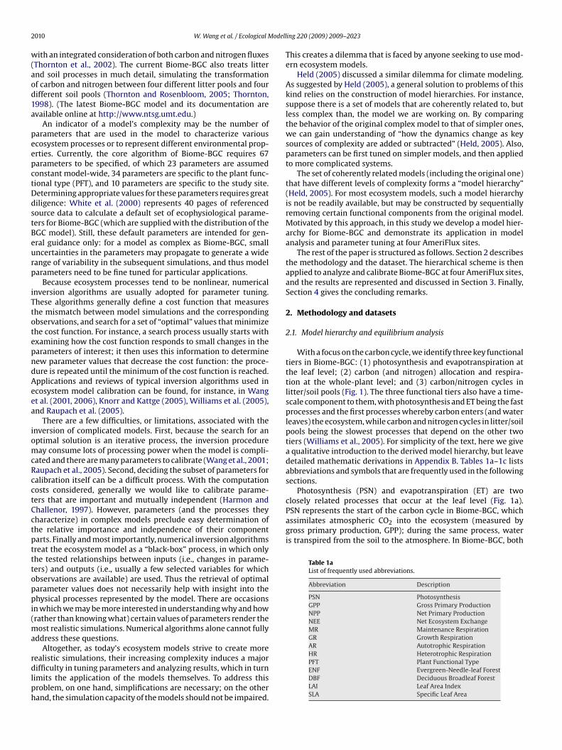

2 odell

w(aod1a

peepctDdstBeurp

iTtotepndAeea

iomcRcctCctptttoppi(ma

rdlph

closely related processes that occur at the leaf level (Fig. 1a).PSN represents the start of the carbon cycle in Biome-BGC, whichassimilates atmospheric CO2 into the ecosystem (measured bygross primary production, GPP); during the same process, wateris transpired from the soil to the atmosphere. In Biome-BGC, both

Table 1aList of frequently used abbreviations.

Abbreviation Description

PSN PhotosynthesisGPP Gross Primary ProductionNPP Net Primary ProductionNEE Net Ecosystem ExchangeMR Maintenance RespirationGR Growth RespirationAR Autotrophic RespirationHR Heterotrophic Respiration

010 W. Wang et al. / Ecological M

ith an integrated consideration of both carbon and nitrogen fluxesThornton et al., 2002). The current Biome-BGC also treats litternd soil processes in much detail, simulating the transformationf carbon and nitrogen between four different litter pools and fourifferent soil pools (Thornton and Rosenbloom, 2005; Thornton,998). (The latest Biome-BGC model and its documentation arevailable online at http://www.ntsg.umt.edu.)

An indicator of a model’s complexity may be the number ofarameters that are used in the model to characterize variouscosystem processes or to represent different environmental prop-rties. Currently, the core algorithm of Biome-BGC requires 67arameters to be specified, of which 23 parameters are assumedonstant model-wide, 34 parameters are specific to the plant func-ional type (PFT), and 10 parameters are specific to the study site.etermining appropriate values for these parameters requires greatiligence: White et al. (2000) represents 40 pages of referencedource data to calculate a default set of ecophysiological parame-ers for Biome-BGC (which are supplied with the distribution of theGC model). Still, these default parameters are intended for gen-ral guidance only: for a model as complex as Biome-BGC, smallncertainties in the parameters may propagate to generate a wideange of variability in the subsequent simulations, and thus modelarameters need to be fine tuned for particular applications.

Because ecosystem processes tend to be nonlinear, numericalnversion algorithms are usually adopted for parameter tuning.hese algorithms generally define a cost function that measureshe mismatch between model simulations and the correspondingbservations, and search for a set of “optimal” values that minimizehe cost function. For instance, a search process usually starts withxamining how the cost function responds to small changes in thearameters of interest; it then uses this information to determineew parameter values that decrease the cost function: the proce-ure is repeated until the minimum of the cost function is reached.pplications and reviews of typical inversion algorithms used incosystem model calibration can be found, for instance, in Wangt al. (2001, 2006), Knorr and Kattge (2005), Williams et al. (2005),nd Raupach et al. (2005).

There are a few difficulties, or limitations, associated with thenversion of complicated models. First, because the search for anptimal solution is an iterative process, the inversion procedureay consume lots of processing power when the model is compli-

ated and there are many parameters to calibrate (Wang et al., 2001;aupach et al., 2005). Second, deciding the subset of parameters foralibration itself can be a difficult process. With the computationosts considered, generally we would like to calibrate parame-ers that are important and mutually independent (Harmon andhallenor, 1997). However, parameters (and the processes theyharacterize) in complex models preclude easy determination ofhe relative importance and independence of their componentarts. Finally and most importantly, numerical inversion algorithmsreat the ecosystem model as a “black-box” process, in which onlyhe tested relationships between inputs (i.e., changes in parame-ers) and outputs (i.e., usually a few selected variables for whichbservations are available) are used. Thus the retrieval of optimalarameter values does not necessarily help with insight into thehysical processes represented by the model. There are occasions

n which we may be more interested in understanding why and howrather than knowing what) certain values of parameters render the

ost realistic simulations. Numerical algorithms alone cannot fullyddress these questions.

Altogether, as today’s ecosystem models strive to create more

ealistic simulations, their increasing complexity induces a majorifficulty in tuning parameters and analyzing results, which in turn

imits the application of the models themselves. To address thisroblem, on one hand, simplifications are necessary; on the otherand, the simulation capacity of the models should not be impaired.

ing 220 (2009) 2009–2023

This creates a dilemma that is faced by anyone seeking to use mod-ern ecosystem models.

Held (2005) discussed a similar dilemma for climate modeling.As suggested by Held (2005), a general solution to problems of thiskind relies on the construction of model hierarchies. For instance,suppose there is a set of models that are coherently related to, butless complex than, the model we are working on. By comparingthe behavior of the original complex model to that of simpler ones,we can gain understanding of “how the dynamics change as keysources of complexity are added or subtracted” (Held, 2005). Also,parameters can be first tuned on simpler models, and then appliedto more complicated systems.

The set of coherently related models (including the original one)that have different levels of complexity forms a “model hierarchy”(Held, 2005). For most ecosystem models, such a model hierarchyis not be readily available, but may be constructed by sequentiallyremoving certain functional components from the original model.Motivated by this approach, in this study we develop a model hier-archy for Biome-BGC and demonstrate its application in modelanalysis and parameter tuning at four AmeriFlux sites.

The rest of the paper is structured as follows. Section 2 describesthe methodology and the dataset. The hierarchical scheme is thenapplied to analyze and calibrate Biome-BGC at four AmeriFlux sites,and the results are represented and discussed in Section 3. Finally,Section 4 gives the concluding remarks.

2. Methodology and datasets

2.1. Model hierarchy and equilibrium analysis

With a focus on the carbon cycle, we identify three key functionaltiers in Biome-BGC: (1) photosynthesis and evapotranspiration atthe leaf level; (2) carbon (and nitrogen) allocation and respira-tion at the whole-plant level; and (3) carbon/nitrogen cycles inlitter/soil pools (Fig. 1). The three functional tiers also have a time-scale component to them, with photosynthesis and ET being the fastprocesses and the first processes whereby carbon enters (and waterleaves) the ecosystem, while carbon and nitrogen cycles in litter/soilpools being the slowest processes that depend on the other twotiers (Williams et al., 2005). For simplicity of the text, here we givea qualitative introduction to the derived model hierarchy, but leavedetailed mathematic derivations in Appendix B. Tables 1a–1c listsabbreviations and symbols that are frequently used in the followingsections.

Photosynthesis (PSN) and evapotranspiration (ET) are two

PFT Plant Functional TypeENF Evergreen-Needle-leaf ForestDBF Deciduous Broadleaf ForestLAI Leaf Area IndexSLA Specific Leaf Area

W. Wang et al. / Ecological Modelling 220 (2009) 2009–2023 2011

Table 1bList of model parameters/state variables.

Symbol Units Description

˛lf 1/yr Annual leaf and fine root turnover fraction˛wd 1/yr Annual live wood turnover fractionˇage 1/yr Annual whole-plant mortality fractionˇfire 1/yr Annual fire mortality fractionr1 (0–1) Allocation ratio—new fine root C:new leaf Cr2 (0–1) Allocation ratio—new stem C:new leaf Cr3 (0–1) Allocation ratio—new live wood C:new total wood Cr4 (0–1) Allocation ratio—new coarse root C:new stem Cdeff m Effective soil depthflnr (0–1) Fraction of leaf nitrogen in Rubiscofpi (0–1) Fraction of actual immobilization (of soil mineral nitrogen) to potential immobilizationgs,max m s−1 Maximum stomatal conductance

arbonitrogearbon–

pblrss“

bG

Fanab,t

Cx kg C/m2, kg C/m2/s CNx g C/m2, g C/m2/s NC:Nx Ratio C

rocesses are calculated on a basis of projected leaf area—they cane fully calculated if the leaf area of the canopy (represented by

eaf area index or LAI) is known. Therefore, if we prescribe LAI butemove the rest of carbon/nitrogen cycles from the model, it shouldtill be able to simulate GPP and ET. Such a simple land-surfacecheme defines the first model in our hierarchy (referred to as the

first-tier” model).

GPP simulated by the first-tier model provides the primary car-on input for the plant-level carbon cycle (Fig. 1b). In particular,PP less maintenance respiration (MR) represents carbon that is

ig. 1. Schematic diagrams of the proposed hierarchy of Biome-BGC, shown as beingnalyzed in model calibration. The three tiers respectively describe (a) photosys-thesis (PSN) and evapotranspiration (ET) at leaf level; (b) carbon and nitrogen cyclest whole-plant level, and (c) carbon and nitrogen cycles in soil and litter pools. Sym-ols and abbreviations are explained in Tables 1a–1c, and the numbers (e.g., ,. . .) indicate the order in which the major carbon/nitrogen fluxes are determinedhrough the calibration process.

stock or carbon flux specified by the subscriptn stock or nitrogen flux specified by the subscriptnitrogen mass ratio

available for allocation, which potentially can be all allocated todifferent vegetation tissues based on the allometric relationshipsamong them (prescribed as model parameters). Accompanying theallocation of carbon, a certain amount of nitrogen must also be allo-cated to vegetation tissues so that their C:N ratios (prescribed asmodel parameters) are maintained. Therefore, the actual allocationis not only determined by available carbon, but also regulated bythe amount of available nitrogen (mainly N uptake from the soil).Normally, the determination of N uptake involves complicated cal-culations of soil/litter processes; however, if we are able to estimatecarbon allocation and N uptake alternatively from a priori informa-tion (e.g., measurements of NPP, litter production rate, and so on),these soil/litter processes may be ignored. Therefore, by removingsoil/litter processes from the original Biome-BGC, the second modelis defined in our hierarchy (referenced as the “second-tier” model).Compared with the first-tier model, the second-tier model incorpo-rates carbon/nitrogen cycles at the plant level, so that the growth ofvegetation (LAI, in particular) is now dynamically simulated insteadof being prescribed.

Finally we examine carbon/nitrogen cycles in litter and soilpools (Fig. 1c). Per Biome-BGC algorithms, dead vegetation tissues(via turnover or whole-plant mortality) are decomposed through aseries of stages and at varying rates, which are represented by mul-tiple litter pools and multiple soil pools (although for simplicity,Fig. 1(c) shows only one litter pool and one soil pool, respectively). Ingeneral, organic matter flow from fast-decaying pools (e.g., litter) to

slow-decaying pools (e.g., soil), during which a proportion of carbonis released to the atmosphere through heterotrophic respiration(HR). The cycling of nitrogen is a bit more complicated: depend-ing on the C:N ratios of the organic matter and its destined pool,

Table 1cList of symbols for ecosystem compartments.

Symbol Ecosystem compartment

lf Leaffr Fine rootlst Live stemdst Dead stemlcr Live coarse rootdcr Dead coarse rootcwd Coarse woody debrislitr1 Litter—labile proportionlitr2 Litter—unshielded cellulose proportionlitr3 Litter—shielded cellulose proportionlitr4 Litter—lignin proportionsoil1 Soil—fast microbial recycling proportionsoil2 Soil—medium microbial recycling proportionsoil3 Soil—slow microbial recycling proportionsoil4 Soil—recalcitrant (slowest) proportion

2012 W. Wang et al. / Ecological Modelling 220 (2009) 2009–2023

Table 2aSite information: general information.

Site Name (Code) Symbol Location Veg. typea Period References

Metolius Intermediate Pine, OR (US-Me2) MT 44.45, −121.56 ENF 2002–2004 Law et al. (2003)N 105.5M 86.41W 90.08

titdtItl(im

s“tistfim2isnat

tviair“ta

ssCt(sw

bctdbaiec((y

iwot Ridge, CO (US-NR1) NR 40.03, −organ Monroe State Forest, IN (US-MMS) MM 39.32, −illow Creek, WI (US-WCr) WC 45.91, −

he decomposition process may release surplus nitrogen (mineral-zation) or may require extra nitrogen (immobilization). Note thathe total soil mineral nitrogen may be lower than that potentiallyemanded by immobilization and vegetation N uptake: in this case,he actual immobilization and the actual uptake will be prorated.ndeed, it is the central task of simulating all soil/litter processeso estimate the balance among nitrogen mineralization, immobi-ization, and N uptake. Therefore, the last model in our hierarchyreferred to as the “third-tier” model) is defined by incorporat-ng the litter/soil processes to the second-tier model. The third-tier

odel is the original, complete version of Biome-BGC.To simplify the analysis of the proposed model hierarchy, this

tudy considers a special status of models, that is, when they are atequilibrium”. Generally, equilibrium of an ecosystem model referso a steady status in which model state variables reach a dynam-cal balance (e.g., dead tissues are replaced by new tissues of theame quantities) so that they do not change at annual or longerime scales. In most experiments, model state variables need to berst “spun up” into equilibrium with respect to the specified cli-ate and ecophysiological conditions (Thornton and Rosenbloom,

005). Ideally, if the model is spun-up using periodic meteorolog-cal data that represent the climatology of the site, the resultingtate variables will have the same seasonal cycles and there will beo interannual variability in them. System equilibrium is generallypproximated by the climatologies (i.e., mean seasonal-cycles) ofhe model state variables brought by spin-up runs.

The analysis and calibration of models can be simplified underhe assumed system equilibrium. For instance, because the stateariables are periodic at system equilibrium, we need to only spec-fy the mean LAI cycle in the first-tier model when calibrating itgainst observed fluxes of ET and GPP. Furthermore, because theres no interannual variability in the state variables, they can beegarded as constant at annual (or longer) time scales. As such, theslow” ecosystem processes (i.e., carbon allocation, soil decomposi-ion, etc.) in the second-tier and the third-tier models can be easilynalyzed with the principle of mass balance.

To illustrate, suppose we have calibrated the first-tier modeluch that it appropriately simulates observed ET and GPP with pre-cribed LAI. Now consider how to calibrate the second-tier model.learly, if we keep model components that are already calibrated inhe first-tier model unchanged, but calibrate the other componentsthat deal with carbon allocation) in a way that they dynamicallyupport a canopy with the same LAI as previously prescribed, thehole second-tier model will be calibrated.

We evaluate the above problem by applying the principle of massalance: under the assumed equilibrium assumption, LAI of theanopy does not change year to year, and carbon annually allocatedo leaf must be the same as the annual leaf-carbon loss throughecay (i.e., turnover or mortality). The latter can be easily estimatedecause the leaf carbon stock is already known (determined by LAInd SLA, specific leaf area), and the rates of turnover and mortal-ty are prescribed model parameters. The same approach can be

xtended to determine carbon stocks and fluxes for other plantomponents, based on their allometric relationships with leavesall of which are model parameters). Subsequently, all major carbonand nitrogen) fluxes in the second-tier model are derived. The anal-sis and calibration of soil/litter processes in the third-tier model

5 ENF 2000–2004 Monson et al. (2002)DBF 2000–2004 Schmid et al. (2000)DBF 2000–2004 Cook et al. (2004)

can be simplified in the same way as above. Therefore, once the first-tier model is calibrated, the calibration of the second-tier and thethird-tier models can be conducted in an analytical fashion, withno numerical inversion techniques involved. This not only simpli-fies model calibration in terms of computation, but also providesinsight into the underlying ecosystem processes and their interac-tions. For the first-tier model, because its LAI is fixed, its calibrationis rather easy and straightforward (see below).

Based on the derivations of the model hierarchy in Appendix B,the following results can be obtained, which provide basic guidanceto analyze the model against observational data in the next section.They are:

• For the first-tier model, a set of three parameters, gs,max (max-imum stomatal conductance), deff (effective soil depth), and flnr(fraction of leaf nitrogen in Rubisco) allows us considerable flex-ibility to calibrate the model against observed fluxes of ET andGPP;

• At system equilibrium, biomass of various vegetation tissues canbe estimated from leaf mass by simple ratios that are fully deter-mined by model parameters describing living-tissue turnover,whole-plant mortality, and allometric allocation;

• By comparing how much nitrogen is required by plant to allocateall available carbon and how much nitrogen is actually allocated,it helps to estimate soil nitrogen availability, and subsequentlyestimate various soil carbon/nitrogen pools.

2.2. Datasets

We demonstrate the application of the proposed modelhierarchy to analyze and calibrate Biome-BGC at two evergreen-needle-forest (ENF) sites and two deciduous-broadleaf-forest (DBF)sites (Table 2a): the Metolius (MT) intermediate-aged pine forest inOregon (Law et al., 2003), the Niwot Ridge (NR) subalpine coniferforest in Colorado (Monson et al., 2002), the Morgan Monroe (MM)deciduous forest in Indiana (Schmid et al., 2000), and the WillowCreek (WC) deciduous forest in Wisconsin (Cook et al., 2004). Allthese sites are part of the AmeriFlux networks, where fluxes ofwater and carbon have been systematically measured hourly (orhalf-hourly) since the late 1990s or early 2000s.

For all sites, we acquired hourly or half-hourly measurementsof ET and GPP for the period of 2000–2004, and processed their8-day averages as described in Yang et al. (2006). In particular, wetreated missing values in the original measurements based on theprocedures of Falge et al. (2001): (1) if more than 70% of data weremissing in an 8-day period, this period was marked as missing; (2)if a particular time of day (e.g., 2 P.M.) was missing in all 8 days, thisperiod was marked as missing; (3) if neither condition 1 nor 2 weremet, we filled missing values with the mean from the non-missingdays: for instance, if a single 2 P.M. value was missing from the 8-day period, it would be filled with the mean of the rest seven 2 P.M.values.

We also acquired site-specific biological data from the Amer-iFlux website (http://public.ornl.gov/ameriflux/). This ancillarydataset, provided by investigators at each flux tower site, includesinformation that describes site physical characteristics, biologicalattributes (of vegetation, litter, and soil), as well as site disturbance

W. Wang et al. / Ecological Modelling 220 (2009) 2009–2023 2013

Table 2bSite information: physical and ecological attributes.

MT NR MM WC

Elevation (m) 1253 3050 275 520Sand (%) 67 59 34 56Clay (%) 7 31 63 33Silt (%) 26 10 3 11Surface Albedo 0.26 0.26 0.20 0.20LAI 3.4 3.6 5.0 5.4Leaf Mass (kg C/m2) 0.37 0.38b 0.22 0.18Fine Root (kg C/m2) 0.28 – 0.27 0.23Wood Mass (kg C/m2) 6.43 7.25 10.40 7.18Leaf Production (kg C/m2/yr) 0.07 0.11 0.21 0.15W

hlottebftibpara((Cf

Table 3Parameters calibrated in the first-tier model. Values in regular-face are originalparameters of Biome-BGC; values in italics indicate the calibrated parameters(shown if they are different from the original ones).

MT NR MM WC

ood Production (kg C/m2/yr) 0.17 – 0.32 0.15

a ENF, evergreen-needle-leaf forest; DBF, deciduous broadleaf forest.b Inferred from LAI and site measured LMA (leaf mass per unit leaf area).

istory. Yet, because the set of information may be originally col-ected for different purposes, the reported biological attributes areften incomplete and sometimes inconsistent at different sites dueo diverse measurement approaches that were involved (althoughhis has been remedied recently by use of standard protocols in Lawt al., 2009). Based on careful evaluation, therefore, we chose sixiological variables (in addition to several site physical attributes)or data-model comparison in this study, which are more consis-ently measured among the studying sites. They include leaf areandex (LAI), leaf biomass, fine-root biomass, aboveground woodiomass, annual leaf production, and annual aboveground woodroduction (Table 2b). These variables are generally reported bysingle value in the ancillary dataset; when multiple values are

eported for a variable, its mean value (between the period of 2000

nd 2004) is used. The finally compiled values of these variablesTable 2b) are consistent with previously reported in the literaturee.g., Law et al., 2003; Schwarz et al., 2004; Turnipseed et al., 2002;urtis et al., 2002; Martin and Bolstad, 2005). For some land sur-

ace parameters (e.g., mean surface albedo) that are missing from

Fig. 2. Mean modeled LAI cycles prescribed in the first-tier model (solid lines)

gs,max (×100) 0.30 0.20 0.30 0.14 0.50 0.25 0.50 0.23deff 1.44 1.31 1.04 1.76 0.93 0.87 1.52 1.09flnr 0.06 0.06 0.04 0.08 0.06 0.08 0.10

the site-specific ancillary dataset, we filled them with values froma high resolution (1 km) global dataset, ECOCLIMAP (Masson et al.,2003).

Last, we compiled daily meteorological fields for the studyingsites using the Surface Observation and Gridding System (SOGS,Jolly et al., 2005), an adaptation of DAYMET (Thornton et al., 1997).Daily maximum/minimum temperature and precipitation are inter-polated based on observations from the nearest Climate PredictionCenter (CPC) and National Weather Service Cooperative ObserverProgram (COOP) climate stations (Jolly et al., 2005). Vapor pressuredeficit (VPD) and incident solar radiation are then calculated basedon algorithms described in Campbell and Norman (1998). Thoughnot shown, the SOGS data are in good agreement with gap-filled sitemeteorology (compiled by Dr. Daniel Ricciuto at Oak Ridge NationalLab, unpublished data).

3. Results and discussion

3.1. First-tier model

The first step to analyze the first-tier model is to specify the mean

seasonal cycle of LAI. This is done by rescaling the mean LAI cyclesobtained from the pre-calibration model experiments (Fig. 2). Forthe ENF sites, the simulated LAI has little seasonal variability, andit is rescaled so that the annual mean LAI matches with site mea-surements (3.4 at MT and 3.6 at NR, respectively; Table 3); for the

. The dash lines indicate in situ observed annual mean or maximum LAI.

2 odell

DwF

dinbilisaiassm

afs

F(

014 W. Wang et al. / Ecological M

BF sites, the mean LAI cycle is rescaled so that its peak matchesith observations (5.0 at MM and 5.4 at WC, respectively; Table 3;

ig. 2).Comparing the seasonal LAI cycles shown in Fig. 2 with other

ata sources (e.g., MODIS LAI product) may indicate some “unreal-stic” features: for instance, modeled LAI at the two DBF sites doesot really level off after it reaches a maturity point in the spring,ut keeps increasing (although at a slower rate) during the grow-

ng season until senescence starts (Fig. 2). Such discrepancies reflectimitations of current Biome-BGC (and other ecosystem modelsn general), for the mechanisms involved in plant phenology andeasonal allocation dynamics are still poorly understood (Waringnd Running, 1998). Because this kind of problem cannot be eas-ly solved by tuning a couple of model parameters, it is not furtherddressed in this study. But we notice that in applications whereimulations of dynamic carbon and nitrogen cycles are not neces-ary, it remains an option to prescribe observed LAI in the first-tierodel.

We used a standard Levenberg–Marquardt algorithm (Press et

l., 1992) to tune the three selected parameters (i.e., gs,max, deff, andlnr). This algorithm searches optimal values for these parameterso that the difference (in term of squares of errors) between the

ig. 3. ET and GPP simulated by the first-tier model with original parameters (dashed bla“OBS”) show the corresponding tower measurements.

ing 220 (2009) 2009–2023

simulated and the observed ET and GPP becomes least. To avoid theinfluence of unit differences between ET and GPP on the results,the two fluxes are normalized by their peak values, respectively.Also, to avoid lengthy iterations, the searching algorithm is set tostop when the reduction in the root-mean-square of errors (RMSE)is less than 0.1% between two successive iterations. We repeatedthis process with various initial values for the selected parameters,and the results consistently converge toward the same direction,indicating a stable solution for each site.

Table 3 shows the fine-tuned parameters (as well as their orig-inal values supplied with Biome-BGC), while Fig. 3 shows modelsimulated ET and GPP fluxes, before and after the calibration, com-pared with observations. As shown, at MT the first-tier model workswell with original parameters, only that the magnitude of ET is abit too high in summer (Fig. 3a). Therefore, the calibration processmoderately decreased gs,max (Table 3). At the other three sites, ETis more distinguishably higher than observations before calibra-tion: it usually reaches 5 mm/day in the summer, while the peaks

of observed ET range between 3 mm/day (NR, WC) and 4 mm/day(MM). This led a reduction by about half in the find-tuned gs,max atthese sites (Table 3). At NR, before calibration ET also shows an ear-lier decrease during the season, suggesting insufficient soil water

ck lines; “ORI”) and calibrated parameters (solid black lines; “CAL”). The gray lines

W. Wang et al. / Ecological Modell

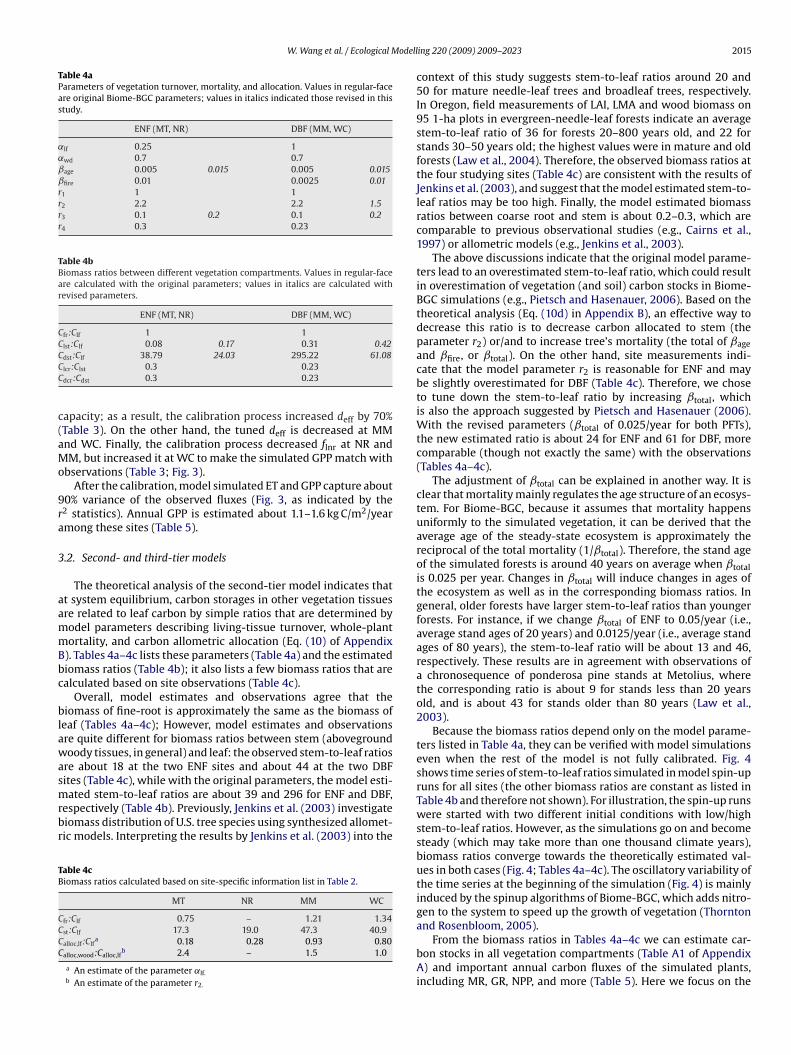
Table 4aParameters of vegetation turnover, mortality, and allocation. Values in regular-faceare original Biome-BGC parameters; values in italics indicated those revised in thisstudy.

ENF (MT, NR) DBF (MM, WC)

˛lf 0.25 1˛wd 0.7 0.7ˇage 0.005 0.015 0.005 0.015ˇfire 0.01 0.0025 0.01r1 1 1r2 2.2 2.2 1.5r3 0.1 0.2 0.1 0.2r4 0.3 0.23

Table 4bBiomass ratios between different vegetation compartments. Values in regular-faceare calculated with the original parameters; values in italics are calculated withrevised parameters.

ENF (MT, NR) DBF (MM, WC)

Cfr:Clf 1 1Clst:Clf 0.08 0.17 0.31 0.42CCC

c(aMo

9ra

3

aammBbc

blawasmrbr

TB

CCCC

dst:Clf 38.79 24.03 295.22 61.08

lcr:Clst 0.3 0.23dcr:Cdst 0.3 0.23

apacity; as a result, the calibration process increased deff by 70%Table 3). On the other hand, the tuned deff is decreased at MMnd WC. Finally, the calibration process decreased flnr at NR andM, but increased it at WC to make the simulated GPP match with

bservations (Table 3; Fig. 3).After the calibration, model simulated ET and GPP capture about

0% variance of the observed fluxes (Fig. 3, as indicated by the2 statistics). Annual GPP is estimated about 1.1–1.6 kg C/m2/yearmong these sites (Table 5).

.2. Second- and third-tier models

The theoretical analysis of the second-tier model indicates thatt system equilibrium, carbon storages in other vegetation tissuesre related to leaf carbon by simple ratios that are determined byodel parameters describing living-tissue turnover, whole-plantortality, and carbon allometric allocation (Eq. (10) of Appendix

). Tables 4a–4c lists these parameters (Table 4a) and the estimatediomass ratios (Table 4b); it also lists a few biomass ratios that arealculated based on site observations (Table 4c).

Overall, model estimates and observations agree that theiomass of fine-root is approximately the same as the biomass of

eaf (Tables 4a–4c); However, model estimates and observationsre quite different for biomass ratios between stem (abovegroundoody tissues, in general) and leaf: the observed stem-to-leaf ratios

re about 18 at the two ENF sites and about 44 at the two DBFites (Table 4c), while with the original parameters, the model esti-

ated stem-to-leaf ratios are about 39 and 296 for ENF and DBF,

espectively (Table 4b). Previously, Jenkins et al. (2003) investigateiomass distribution of U.S. tree species using synthesized allomet-ic models. Interpreting the results by Jenkins et al. (2003) into the

able 4ciomass ratios calculated based on site-specific information list in Table 2.

MT NR MM WC

fr:Clf 0.75 – 1.21 1.34st:Clf 17.3 19.0 47.3 40.9alloc,lf:Clf

a 0.18 0.28 0.93 0.80alloc,wood:Calloc,lf

b 2.4 – 1.5 1.0

a An estimate of the parameter ˛lf.b An estimate of the parameter r2.

ing 220 (2009) 2009–2023 2015

context of this study suggests stem-to-leaf ratios around 20 and50 for mature needle-leaf trees and broadleaf trees, respectively.In Oregon, field measurements of LAI, LMA and wood biomass on95 1-ha plots in evergreen-needle-leaf forests indicate an averagestem-to-leaf ratio of 36 for forests 20–800 years old, and 22 forstands 30–50 years old; the highest values were in mature and oldforests (Law et al., 2004). Therefore, the observed biomass ratios atthe four studying sites (Table 4c) are consistent with the results ofJenkins et al. (2003), and suggest that the model estimated stem-to-leaf ratios may be too high. Finally, the model estimated biomassratios between coarse root and stem is about 0.2–0.3, which arecomparable to previous observational studies (e.g., Cairns et al.,1997) or allometric models (e.g., Jenkins et al., 2003).

The above discussions indicate that the original model parame-ters lead to an overestimated stem-to-leaf ratio, which could resultin overestimation of vegetation (and soil) carbon stocks in Biome-BGC simulations (e.g., Pietsch and Hasenauer, 2006). Based on thetheoretical analysis (Eq. (10d) in Appendix B), an effective way todecrease this ratio is to decrease carbon allocated to stem (theparameter r2) or/and to increase tree’s mortality (the total of ˇage

and ˇfire, or ˇtotal). On the other hand, site measurements indi-cate that the model parameter r2 is reasonable for ENF and maybe slightly overestimated for DBF (Table 4c). Therefore, we choseto tune down the stem-to-leaf ratio by increasing ˇtotal, whichis also the approach suggested by Pietsch and Hasenauer (2006).With the revised parameters (ˇtotal of 0.025/year for both PFTs),the new estimated ratio is about 24 for ENF and 61 for DBF, morecomparable (though not exactly the same) with the observations(Tables 4a–4c).

The adjustment of ˇtotal can be explained in another way. It isclear that mortality mainly regulates the age structure of an ecosys-tem. For Biome-BGC, because it assumes that mortality happensuniformly to the simulated vegetation, it can be derived that theaverage age of the steady-state ecosystem is approximately thereciprocal of the total mortality (1/ˇtotal). Therefore, the stand ageof the simulated forests is around 40 years on average when ˇtotalis 0.025 per year. Changes in ˇtotal will induce changes in ages ofthe ecosystem as well as in the corresponding biomass ratios. Ingeneral, older forests have larger stem-to-leaf ratios than youngerforests. For instance, if we change ˇtotal of ENF to 0.05/year (i.e.,average stand ages of 20 years) and 0.0125/year (i.e., average standages of 80 years), the stem-to-leaf ratio will be about 13 and 46,respectively. These results are in agreement with observations ofa chronosequence of ponderosa pine stands at Metolius, wherethe corresponding ratio is about 9 for stands less than 20 yearsold, and is about 43 for stands older than 80 years (Law et al.,2003).

Because the biomass ratios depend only on the model parame-ters listed in Table 4a, they can be verified with model simulationseven when the rest of the model is not fully calibrated. Fig. 4shows time series of stem-to-leaf ratios simulated in model spin-upruns for all sites (the other biomass ratios are constant as listed inTable 4b and therefore not shown). For illustration, the spin-up runswere started with two different initial conditions with low/highstem-to-leaf ratios. However, as the simulations go on and becomesteady (which may take more than one thousand climate years),biomass ratios converge towards the theoretically estimated val-ues in both cases (Fig. 4; Tables 4a–4c). The oscillatory variability ofthe time series at the beginning of the simulation (Fig. 4) is mainlyinduced by the spinup algorithms of Biome-BGC, which adds nitro-gen to the system to speed up the growth of vegetation (Thornton

and Rosenbloom, 2005).

From the biomass ratios in Tables 4a–4c we can estimate car-bon stocks in all vegetation compartments (Table A1 of AppendixA) and important annual carbon fluxes of the simulated plants,including MR, GR, NPP, and more (Table 5). Here we focus on the

2016 W. Wang et al. / Ecological Modelling 220 (2009) 2009–2023

Fig. 4. Evolutions of biomass ratios in model “spin-up” simulations for (a) EvergreenNtrd

tCgaaci

TC

GMCCGNC

Table 6Nitrogen fluxes (units: g N/m2/year) and fpi estimated in the third-tier model.

MT NR MM WC

Npot,alloc 12.8 7.9 17.9 23.9Nact,alloc 4.9 5.2 13.1 14.4Nretrans 1.7 1.8 4.6 5.1Nuptk 3.2 3.4 8.5 9.2fpi 25% 43% 48% 38%Nmin 15.6 17.0 29.4 32.2Nimmob 12.8 13.9 21.1 23.1

eedle Forest and (b) Deciduous Broadleaf Forest. The two panels (from top to bot-om) show biomass ratios between: (1) live stem and leaf; (2) dead stem and leaf,espectively. The notations of “run1” and “run2” indicate model experiments withifferent initial conditions.

wo fluxes, Cpot,alloc (carbon available for potential allocation) andact,alloc (actually allocated carbon), for they help evaluate nitro-en limitation of the simulated ecosystem. For instance, at MT

2

nnual GPP is estimated at about 1.63 (kg C/m /year) and MR isbout 0.48 (kg C/m2/year); therefore, about 1.2 (kg C/m2/year) ofarbon is available for allocation (Cpot,alloc; Table 5). However, thendependently estimated Cact,alloc is only about 0.5 (kg C/m2/year),

able 5arbon fluxes (units: kg C/m2/year) estimated in the second-tier model.

MT NR MM WC

PP 1.63 1.14 1.48 1.61R 0.48 0.48 0.47 0.34

pot,alloc 1.15 0.66 1.01 1.27act,alloc 0.49 0.52 0.84 0.95R 0.11 0.12 0.19 0.22PPa 0.38 0.40 0.65 0.73act,alloc/Cpot,alloc 0.43 0.79 0.83 0.75

a Calculated as Cact,alloc less GR.

Nloss,vol 0.16 0.17 0.30 0.33Nloss,fire 0.34 0.29 0.29 0.38Ninput 0.50 0.46 0.59 0.71

approximately 43% of Cpot,alloc (Table 5). Therefore, carbon allo-cation at MT (in the model) is considerably limited by nitrogenavailability. Nitrogen limitation, although to less degrees, is alsofound at the other sites (Table 5).

Limited nitrogen availability is more formally quantified by thestate variable fpi (fraction of potential immobilization; Eq. (13) ofAppendix B) in Biome-BGC. Based on the carbon budget of vegeta-tion (Table 5) and the associated C:N ratios (Table A2), we estimatethe corresponding nitrogen budget and fpi for all sites (Table 6). AtMT, the simulated vegetation would need about 12.8 (g N/m2/yr) ofnitrogen (Npot,alloc) in order to allocate all its available carbon; how-ever, the amount of nitrogen (Nact,alloc) it can actually get is about4.9 (g N/m2/yr), of which 1.7 (g N/m2/yr) is from retranslocation(Nretrans) and about 3.2 (g N/m2/yr) is uptake from the soil (Nuptk;Table 6). Therefore, fpi (estimated as the ratio between Nuptk andNpot,alloc) is about 25% (Table 6). The estimated fpi ranges 38%–48%at the other sites (Table 6).

Once fpi is known, we can estimate all carbon/nitrogen stocksand fluxes in the soil/litter pools. The estimated soil/litter carbonstocks are listed in Table A1 (Appendix A). The estimated nitrogenstocks, though not directly shown, can be inferred based on thecarbon stocks (Table A1) and the C:N ratios (Table A2). Here weexamine the estimated nitrogen fluxes for the rest of the ecosys-tem (Table 6). As shown, annually mineralized nitrogen is about 16(g N/m2/yr) at NR and MT, and about 30 (g N/m2/yr) at MM and WC;the corresponding immobilized nitrogen is about 13 (g N/m2/yr)and about 22 (g N/m2/yr), respectively, accounting for 80% of min-eralization at NR and MT, and 60% of mineralization at MM andWC. Most of the remaining mineralized nitrogen is taken up bythe plants (Table 6), but a small proportion of nitrogen is releasedfrom the system, mainly through volatilization (Nloss,vol) and fire(Nloss,fire). The annual loss of nitrogen is about 0.5 (g N/m2/yr) atMT and NR, and about 0.6–0.7 (g N/m2/yr) at MM and WC (Table 6).The loss of nitrogen must be compensated by the input of nitro-gen in to the system, which determines the overall rate of nitrogendeposition and fixation (Ninput) at each site (Table 6).

The determination of Ninput represents the last step in analyzingthe second- and the third-tier model. With this information, as wellas the parameters fine-tuned in the first-tier model, we then run thefull BGC-Biome model to verify the calibrations and analyses dis-cussed above. Fig. 5 shows the simulated ET, GPP, and LAI, along withthe corresponding observations. As shown, the simulated LAI is con-sistent with that was prescribed in the first-tier model, which alsodictates the agreement between the simulated ET and GPP fluxesand the observations (Fig. 5). Indeed, the final simulated ET and GPPare almost identical to those simulated by the calibrated first-tiermodel (not shown).

We also compare the simulated carbon stocks of the ecosys-

tem with those previously estimated (Table A1 of Appendix A).Fig. 6 shows the scatter plots of the carbon stocks at all sites,with the abscissa (x-) and ordinate (y-) coordinates represent-ing theoretical estimates and model simulations, respectively.

W. Wang et al. / Ecological Modelling 220 (2009) 2009–2023 2017

ack lin

Tpfdutet

Fig. 5. ET, GPP, and LAI simulated by the calibrated Biome-BGC model (solid bl

here is good agreement between the two sets of results: all thelotted points, ranging from 0.01 (kg C/m2, in living wood and

ast-decaying soil pools) to 16 (kg C/m2, in dead wood and slow-

ecaying soil pools), lie upon or adjacent to the 1-to-1 line (Fig. 6,pper panels). The only outliers are the two fast-decaying lit-er/soil pools (litr1 and soil1) at the two DBF sites, where thestimates are lower than simulations (Fig. 6). This is caused byhe fact that these two carbon pools are small and are subject

es; “BGC”), compared with the tower measurements (solid gray lines; “OBS”).

to relatively high seasonal variability (not shown), and thus theestimation of the annual mean carbon stocks is biased. How-ever, this problem does not affect the estimation of the annual

effluxes from these pools, which are constrained by the carbonbalance relationship and thus by the influxes from the upstreamcarbon pools. Therefore, estimation errors of the two compart-ments do not propagate to the estimates of other soil/litter pools(Fig. 6).

2018 W. Wang et al. / Ecological Modelling 220 (2009) 2009–2023

F (of thm

3

ameo““Himtsrtetscim

ot(at

ig. 6. Comparison between carbon stocks estimated by the hierarchical analysisodel.

.3. Discussion

Above we demonstrated how to apply the proposed model hier-rchy to tune a few selected parameters of Biome-BGC so that theodel can closely simulate observed ET, GPP, LAI, and some other

cological attributes (e.g., aboveground biomass). Because of theptimization techniques involved, this process is sometimes calledparameter optimization”, and the obtained parameters are calledoptimal parameters” (e.g., Jackson et al., 2003; Mo et al., 2008).owever, the word “optimization” here may not be interpreted

n a physiologically meaningful way. For instance, in the first-tierodel the fine-tuned maximum stomatal conductance (gs,max) at

he two DBF sites is about half of its original values (0.0025 m/s ver-us 0.0050 m/s; Table 3): the new gs,max renders better simulationesults, but it is discernibly lower than values commonly reported inhe literature (e.g., Larcher, 2003). Although this discrepancy can bexplained by the fact that there are considerable site-to-site varia-ions in gs,max (Kelliher et al., 1995) and thus the adjusted values aretill valid, it may also suggest other issues in the model that are notovered by the current analysis. Indeed, it is found that when LAIs high (3 or greater), light-use efficiency in the current Biome-BGC

ay be too high (unpublished results).The hierarchical analysis scheme allows us to diagnose some

ther aspects of the model. In the second-tier model, for instance,he modeled maintenance respiration (MR) and growth respirationGR) is usually not sufficient to explain the difference between GPPnd NPP (Table 5), and an additional pathway must be introducedo help remove the surplus carbon when necessary (see Appendix

e second- and the third-tier models) and simulated by the calibrated Biome-BGC

B for details). Reasons for this discrepancy remain unknown: it mayindicate that our knowledge of respiration is still very limited, oralternatively, it suggests that NPP is underestimated. In the lattercase, because the simulated aboveground NPP is calibrated basedon observations, it also suggests that a portion of NPP may not becaptured by the current measurements. Furthermore, in currentBiome-BGC insufficient allocation is always attributed to restrictednitrogen availability. Although it is probably true because temper-ate forests are generally nitrogen limited (Magnani et al., 2007), theextent to which nitrogen is limiting vegetation growth in the modelis however questionable for that as discussed above, any bias in sim-ulated respiration can lead to incorrect nitrogen budget. Limited bythe used dataset, this study does not examine the soil nitrogen bud-get of Biome-BGC with observations. We recognize this limitation,and expect to address it in the future.

Finally, it needs to be pointed out that the analysis of the second-and the third-tier model in this study is solely based on the equilib-rium assumption, while such equilibrium can hardly be observedat individual flux-tower sites (including the four sites in this study).Indeed, site studies indicate that old-growth forests (with agesof hundreds of years) may still accumulate carbon (Luyssaert etal., 2008). One reason for this mismatch may be the fact that thesequestration of atmospheric carbon is a “slow-in, rapid-out” pro-

cess, and the “rapid-out” carbon fluxes (released by disturbancessuch as fire) are difficult to monitor by flux towers (Körner, 2003).On the other hand, vegetation simulated by Biome-BGC (or othersimilar ecosystem models) inherently accounts for disturbanceslike fire and mortality of various causes, and it thus represents

odell

almmiofmtaade

4

isttperwetted(datltsopnpie

fpibbacaadau

Bm

A

Mt

brate the proposed model hierarchy of Biome-BGC. It identifies theparameters for calibration of ET and GPP in the first-tier model and

W. Wang et al. / Ecological M

statistical average of forests of different ages (as discussed ear-ier in the paper). For this reason, in calibrating the second-tier

odel we compared the derived biomass ratios not only to siteeasurements, but also to allometric models (Jenkins et al., 2003),

n order to make the analysis more general. Nevertheless, we rec-gnize that the equilibrium analysis approach alone is insufficientor non-steady ecosystems (e.g., forests that have undergone recent

ajor disturbances or partial disturbances such as ground fire orhinning). In this case, the dynamic characteristics of the modelround the equilibrium must be taken into account (Thornton etl., 2002). Dynamical analysis of ecosystem models can also be con-ucted under the proposed hierarchical model scheme, which wexpect to address in future studies.

. Conclusions

This study develops a hierarchical scheme to analyze and cal-brate the terrestrial ecosystem model Biome-BGC. Under thischeme, Biome-BGC is divided into three functionally cascadediers. The first-tier model focuses on ecophysiological processes athe leaf level. It allows LAI in the model to be specified based on ariori information (usually observations), and simulates observedvapotranspiration and photosynthesis with the prescribed LAI. Theestriction on prescribed LAI is then lifted in the following two tiers,hich analyze how carbon and nitrogen is cycled in the simulated

cosystem to dynamically support the prescribed canopy. In par-icular, the second-tier model considers the cycling of carbon athe whole-plant level. Based on the principle of carbon balance, itstimates biomass storage in all vegetation components and theiremands for annual carbon allocation directly from the prescribedand thus observed) LAI and the allometric allocation relationshipsescribed in Biome-BGC. By comparing carbon that is potentiallyvailable for allocation with carbon that is actually allocated, thisier of the model also evaluates how vegetation carbon allocation isimited by soil nitrogen availability. The third-tier model extendshe methodology of the second tier to analyze carbon/nitrogentocks and fluxes in all litter/soil pools. It calculates nitrogen fluxesf mineralization and immobilization resulting from the decom-osition of soil organic matter and litter biomass. It also estimatesitrogen fluxes that are escaped from the ecosystem during theserocesses, and finally, determines how much nitrogen must be

nput annually to meet the total nitrogen balance of the simulatedcosystem.

This model hierarchy is examined with model experiments atour AmeriFlux sites. The results indicate that this approach sim-lifies the calibration of Biome-BGC, and also helps to diagnose the

nternal status of the model, which is difficult by conventional cali-ration algorithms. In addition, the results indicate good agreementetween carbon/nitrogen stocks estimated by the derived methodsnd those by model simulations, suggesting they may find appli-ations in solving the problem of model spin-up, especially forpplications over large regions. However, because these methodsre derived based on the assumption of equilibrium, they cannotirectly be applied to analyze non-steady ecosystems. Future effortsre needed to analyze the dynamic characteristics of the modelnder the proposed hierarchical scheme.

Finally, although this paper mainly focuses on analyzing Biome-GC, the general concept and methodology developed in this studyay help analyze other similar ecosystem models as well.

cknowledgements

This research was supported by funding from NASA’s Scienceission Directorate through EOS. The views expressed herein are

hose of the authors and do not necessarily reflect the views of

ing 220 (2009) 2009–2023 2019

NASA. Flux tower measurements were funded by the Departmentof Energy, the National Oceanic and Atmospheric Administration,the National Space Agency (NASA) and the National Science Foun-dation. The Metolius research was supported by the Office ofScience (BER), U.S. Department of Energy (DOE, Grant no. DE-FG02-06ER64318). Special thanks to Drs. Russell Monson, Danilo Dragoni,and Kenneth Davis for providing flux data at Niwot Ridge, Mor-gan Monroe State Forest, and Willow Creak. Research at the MMSFis supported by the Office of Science (BER), US-DOE, Grant No.DE-FG02-07ER64371. The authors are grateful to two anonymousreviewers for their constructive comments and suggestions. Wealso thank Dr. Jennifer Dungan for helpful feedback on an earlierversion of this manuscript. W. Wang thanks Dr. Masao Kanamitsufor initial discussions on the Held (2005) paper.

Appendix A. Supplemental tables

Table A1Estimated carbon stocks in ecosystem compartments (Unit: kg C/m2).

MT NR MM WC

lf 0.28 0.30 0.17 0.19fr 0.28 0.30 0.17 0.19lst 0.047 0.050 0.071 0.079dst 6.81 7.21 10.18 11.18lcr 0.014 0.015 0.014 0.016dcr 2.04 2.16 2.04 2.24cwd 4.51 4.84 2.05 3.54litr1 0.010 0.004 0.003 0.007litr2 0.42 0.18 0.09 0.19litr3 0.20 0.09 0.04 0.07litr4 0.76 0.34 0.16 0.35soil1 0.010 0.011 0.008 0.016soil2 0.19 0.21 0.11 0.22soil3 1.95 2.16 1.13 2.14soil4 12.25 13.61 7.12 13.51

Table A2C:N ratios of ecosystem compartments (Unit: kg C/kg N)a.

ENF (MT, NR) DBF (MM, WC)

C:Nlf 42 24C:Nlf,dead 93 49C:Nfr 42 42C:Nlst , C:Nlcr 50 50C:Ndst, C:Ndcr 729 442C:Ncwd 721 437C:Nlitr1 59 46C:Nlitr2 153 75C:Nlitr3 56 42C:Nlitr4 114 65C:Nsoil1 12 12C:Nsoil2 12 12C:Nsoil3 10 10C:Nsoil4 10 10

a C:N ratios of vegetation and soil pools are prescribed model parameters, whileC:N ratios of litter and CWD pools are not prescribed but estimated using algorithmsdiscussed in the text.

Appendix B. Derivation of the model hierarchy

This appendix discusses in detail how to analyze and cali-

derives mass-balance equations to estimate carbon/nitrogen fluxesin the second-tier and the third-tier models. Yet it is impossible tocover all components of Biome-BGC in this paper. For more detaileddiscussions of Biome-BGC, we refer the reader to Thornton (1998)and Thornton et al. (2002).

2 odell

B

c

ssflogesth

eb

E

wswta

sibsp

g

wg

E

crmtgFhk

ebC

A

wcw

g

o

tAhfi

020 W. Wang et al. / Ecological M

.1. First-tier model

The first-tier model simulates ET and GPP with prescribed LAI. Toalibrate the model, we consider the water-cycle component first.

Biome-BGC simulates water fluxes evaporated from the soilurface and vegetation canopy (i.e., intercepted precipitation), tran-pired by vegetation, and sublimated from the snowpack. Of theseuxes, sublimation of snow and evaporation of intercepted waterccur under certain conditions (i.e., when there is snow on theround and on rainy days, respectively), which can be relativelyasily differentiated in observations. In addition, for well-vegetatedites, evaporation from the soil surface is generally less importanthan transpiration from canopy. Therefore, the main focus here isow to calibrate the transpiration of soil water by vegetation.

Biome-BGC uses the Penman–Monteith equation to estimatevapotranspiration rate (ET, per projected leaf area), which can alsoe represented as a diffusive process (Sellers et al., 1997):

T = gv[e∗(Ts) − ea]�cp

��, (1)

here gv is the leaf-level conductance for water vapor, e*(Ts) is theaturation water vapor pressure at leaf temperature Ts, ea is theater vapor pressure of the ambient air; �, cp, �, and � represent

he density and specific heat of air, the latent heat of evaporation,nd the psychrometric constant.

In Eq. (1), leaf water conductance (gv) is mainly regulated bytomatal conductance (gs), which is modeled as a product of a max-mum value (gs,max) and a series of multiplicative regulators (valuedetween 0 and 1) that respond to incident radiation (R), vapor pres-ure deficit (VPD), minimum temperature (Tmin), and soil waterotential (� ), that is,

s = m(R) · m(VPD) · m(Tmin) · m(� ) · gs,max (2)

here m represents the regulator functions. Approximate gv withs by substituting Eq. (2) into Eq. (1), giving

T = m(R)m(VPD)m(Tmin)m(� )gs,max[e∗(Ts) − ea]�cp

��. (3)

In Eq. (3), �, cp, �, and � are physical constants; VPD and Tmin arelimate variables that are externally determined; and the incidentadiation, R, and the vapor pressure difference, e*(Ts) − ea, are alsoainly determined by climate variables. Therefore, an effective way

o calibrate ET is to adjust the maximum stomatal conductance,s,max, and another parameter that affects soil water potential (� ).or the latter, because variations of � strongly depend on soil water-olding capacity, we choose the effective depth of soil (deff, alsonown as the rooting depth) as the second parameter to tune.

Next, we consider the photosynthesis component. Biome-BGCstimates the carbon assimilation rate (A, per projected leaf area)y constraining the Farquhar model (Farquhar et al., 1980) with aO2 diffusion equation,

= gc(Ca − Ci), (4)

here Ca and Ci represent atmospheric and intracellular CO2 con-entration, respectively; gc is the leaf-level conductance for CO2,hich is related to the conductance of water (gv) by

c = gv

1.6. (5)

Therefore, photosynthesis is closely related to transpiration, andnce gv is determined, gc is determined as well.

In Biome-BGC, Eq. (4) is substituted into the Farquhar modelo eliminate the unknown variable Ci, so that the assimilation rate

can be solved. For brevity, the Farquhar model is not presentedere (but see Farquhar et al., 1980 for detailed discussion). It is suf-cient to indicate that A mainly depends on leaf temperature and

ing 220 (2009) 2009–2023

leaf nitrogen, which influence the specific activity and the amountof the Rubisco enzyme, respectively (Thornton et al., 2002). Becausetemperature is a climate variable, we consider how to adjust leafnitrogen, which is determined by specific leaf area (SLA), the leafC:N ratio (C:Nleaf), and the fraction of leaf nitrogen in the Rubiscoenzyme (flnr). Of these variables, flnr has the smallest effect on therest of carbon/nitrogen cycle (see below), and thus it is chosen asthe third parameter to calibrate the rate of photosynthesis.

B.2. Second-tier model

In the second-tier model, we focus on analyzing the plant-levelcarbon/nitrogen cycles at system equilibrium. First, we consider thequestion of how much carbon is required to support leaf growth,given the assumption that maximum LAI (for DBF) or mean LAI(for ENF) does change year to year. (For simplicity, below we usemaximum LAI as the example to derive the equations. For evergreenforests, LAI simulated by Biome-BGC is almost constant, and thusannual maximum LAI closely approximates as annual mean LAI).Based on the principle of mass balance, carbon allocated to leavesmust be balanced by carbon lost via litterfall and mortality, that is,

Cl,alloc = (1 + fgr) · (˛ + ˇ) · Cl,max, (6)

where Cl,alloc indicates newly allocated leaf carbon; Cl,max denotesleaf carbon corresponding to maximum LAI; ˛ and ˇ represent theannual rates of litterfall and overall mortality (the total of ˇage andˇfire shown in Tables 1a–1c), respectively; and fgr indicates the frac-tion of carbon that is respired during the growth process, whichis assumed to be 0.3 in Biome-BGC. Note that Eq. (6) was derivedfor evergreen forests based on the assumption that leaf carbon isalways Cl,max. For deciduous forests, because trees shed all theirleaves every year, the annual total loss of leaf carbon is approxi-mately Cl,max, that is, the sum of ˛ and ˇ is 1.

Eq. (6) indicates that Cl,alloc can be estimated based on Cl,max.At the same time, according to the allometric allocation schemeassumed in Biome-BGC, carbon allocated to other vegetation com-partments is directly or indirectly proportional to Cl,alloc. For woodyspecies, these compartments include fine root, live/dead stem, andlive/dead coarse root, and the corresponding carbon fluxes are:

Cfr,alloc = r1 · Cl,alloc (fine roots) (7a)

Clst,alloc = r2 · r3 · Cl,alloc (live stem) (7b)

Cdst,alloc = r2 · (1 − r3) · Cl,alloc (dead stem) (7c)

Clcr,alloc = r4 · r2 · r3 · Cl,alloc (live coarse root) (7d)

Cdcr,alloc = r4 · r2 · (1 − r3) · Cl,alloc (dead coarse root) (7e)

where rs denote allometric parameters (Tables 1a–1c). Together, thetotal amount of annually allocated carbon is estimated as:

Cact,alloc = (1 + r1 + r2 + r2r4) · Cl,alloc. (8)

and the annual growth respiration (GR) is:

GR = fgr

1 + fgr· Cact,alloc ≈ 0.23 · Cact,alloc, (9)

where a constant value of 0.3 is assumed for the parameter fgr.As in Eq. (6), we can write carbon balance equations for all the

plant compartments described above. Because the newly allocatedcarbon to these compartments is already known (Eq. (7)), these bal-ance relationships can be inverted to estimate their carbon stocks interm of Cl,max. For live tissues (i.e., fine roots, live stem/coarse root),

because they go through similar aging processes (e.g., litterfall orturnover) as leaves, the following relationships can be formulated:

Cfr,max = ˛l + ˇ

˛fr + ˇ· r1 · Cl,max (fine roots) (10a)

odell

C

C

witpe

sst

C

C

C

cBwf

M

wof

af

C

gaa(bebn

B

lt

tt

W. Wang et al. / Ecological M

lst = ˛l + ˇ

˛lst + ˇ· r2 · r3 · Cl,max (live stem) (10b)

lcr = ˛l + ˇ

˛lcr + ˇ· r4 · r2 · r3 · Cl,max (live coarse root) (10c)

here ˛s represent the rate of litterfall/turnover of the correspond-ng tissues. For dead woody tissues (i.e., dead stem/coarse root),hey gain carbon from the turnover process of their live counter-arts, and they lose carbon only when the whole plant dies. Thequations to estimate their biomass are thus:

Cdst =[

˛l + ˇ

ˇ· r2 · (1 − r3) + ˛lst

ˇ· ˛l + ˇ

˛lst + ˇ· r2 · r3

]· Cl,max

(dead stem) (10d)

Cdcr =[

˛l + ˇ

ˇ· r4 · r2 · (1 − r3) + ˛lcr

ˇ· ˛l + ˇ

˛lcr + ˇ· r4 · r2 · r3

]· Cl,max

(dead coarse root) (10e)

In Biome-BGC, the default litterfall rate of fine roots (˛fr) is theame as leaves (˛l), and the turnover rate of live stem (˛lst) is theame as live coarse root (˛lcr). It thus can be derived from Eq. (10)hat:

fr,max = r1 · Cl,max (fine roots) (10a′)

lcr = r4 · Clst (live coarse root) (10c′)

dcr = r4 · Cdst (dead coarse root) (10e′)

Eq. (10) allows us to estimate carbon stocks for all vegetationompartments. From the corresponding C:N ratios prescribed iniome-BGC, their nitrogen content is also determined. On this basis,e can further calculate the annual maintenance respiration (MR)

or these components by (Thornton, 1998):

R = 0.218 · N · Q (T−20)/1010 (11)

here N and T indicate the nitrogen content and the temperaturef the component, respectively; the Q10 factor is assumed to be 2.0or all components.

Based on the estimated annual GPP (from the first-tier model)nd MR (Eq. (11)), the amount of carbon that is potentially availableor allocation (Cpot,alloc) can be estimated as,

pot,alloc = GPP − MR (12)

On the other hand, the actually allocated carbon, Cact,alloc, isiven by Eq. (8). Per Biome-BGC algorithms, Cact,alloc is the sames Cpot,alloc only if vegetation growth is not restrained by avail-ble nutrients (i.e., mineral nitrogen); otherwise the surplus carbonCpot,alloc − Cact,alloc) is removed from the system1. The differenceetween Cpot,alloc and Cact,alloc thus provides a measure by which tovaluate whether/how the simulated vegetation growth is limitedy nitrogen availability. This subject will be further discussed in theext section.

.3. Third-tier model

The decomposition of litter and soil organic matter is generallyimited by soil mineral nitrogen. Per Biome-BGC algorithms, thewo main demands for mineral nitrogen are plant uptake and soil

1 In the original Biome-BGC, the surplus carbon is removed by reducing GPP byhe corresponding amount; in this study, however, we revised the model to removehe surplus carbon by increasing the total amount of autotrophic respiration.

ing 220 (2009) 2009–2023 2021

immobilization. When soil mineral nitrogen (Nsmin) cannot meetthe total demands from the two components, the actual allocations(i.e., Nact,uptk and N,act,immb) are made proportionally to their poten-tial demands (i.e., Npot,uptk and Npot,immb). Therefore, when Nsmin islimited, the following ratios are the same:

fpi = Nact,immb

Npot,immb= Nact,uptk

Npot,uptk= Ns, min

Npot,immb + Npot,uptk, (13)

where fpi stands for “the fraction of potential immobilization”, astate variable defined in Biome-BGC.

Eq. (13) indicates that fpi can be estimated from nitrogen uptakeby vegetation. Indeed, Npot,uptk is directly estimated from Cpot,alloc(Eq. (12)) based on the C:N ratios of different vegetation compart-ments. Similarly, the nitrogen actually allocated (Nact,alloc) can beestimated from Cact,alloc (Eq. (8)). Finally, to estimate Nact,uptk fromNact,alloc we need to deduct the portion of nitrogen (Ntrans) thatis retranslocated within the plant2. Based on the carbon/nitrogenstocks in different vegetation compartments (estimated in thesecond-tier model) and their decay rate, the calculation of Ntrans

is straightforward and therefore neglected here.Once fpi is known, we are ready to estimate carbon/nitrogen

stocks in all the four litter pools (and a coarse woody debris pool)and the four soil pools defined in Biome-BGC. These pools are linkedin a manner that carbon and nitrogen always flow from faster-decaying pools to slower decaying pools, and thus the inflow ofa pool is determined solely by the outflow of its upstream pools (adetailed diagram can be found in Thornton and Rosenbloom, 2005).Because the most-upstream pools (i.e., plant compartments) are allknown, carbon/nitrogen stocks in these soil/litter pools, as well asthe fluxes among them, can be sequentially estimated.

To illustrate, we consider the case of the labile litter pool, whichis the first litter pool in Biome-BGC. This pool contains the labileportion of the leaf and fine root litter, and a part of newly allocatedcarbon/nitrogen that enters the pool when the whole plant dies.Therefore, the total inflow to the labile litter pools is:

X inflowlitr1 = plab · [(˛l + ˇage) · Xl,max + (˛fr + ˇage) · Xfr,max]

+ ˇage · 0.5 · Xact,alloc (14)

where X denotes either “C” (carbon) or “N” (nitrogen) and plab is amodel parameter that represents the labile proportion of leaf andfine root litter. The constant factor (0.5) in the last term of Eq. (14)represents the proportion of allocated carbon and nitrogen that isstored for vegetation growth in the next growing season (Thornton,1998). Note that all variables in Eq. (14) are known.

The outflow of the labile pool is induced by fire and by decom-position, that is,

Xoutflowlitr1 = (ˇfire + fpi · mcorr · klitr1) · Xlitr1 (15)

where ˇfire indicates fire-induced mortality; klitr1 is the basedecomposition rate of this litter pool (specified by model param-eters), while mcorr represents the regulation of climate variationson the decomposition rate. The calculation of mcorr mainly involvessoil temperature and soil moisture, which are determined based onthe results of the first-tier model.

At system equilibrium, the inflow of carbon and nitrogen in Eq.(14) must be balanced by the outflow in Eq. (15). Therefore, the only

unknown variable in Eq. (15), Xlitr1, is determined. Subsequently, thecomponents of the outflow [on the right-hand-side of Eq. (15)] canbe calculated, which then are used to estimate the heterotrophicrespiration (HR), fire emissions (of carbon and nitrogen), and the

2 In Biome-BGC, Ntrans is calculated for turnover leaf and wood (stem and coarseroot) by the N difference between living leaf/wood and dead leaf/wood, which havedifferent C:N ratios.

2 odell

ci

tlosmebgs(nin

upgtgpnme

nenmwtatfe

(cfe

R

C

C

C

C

C

F

F

H

H

I

022 W. Wang et al. / Ecological M

arbon/nitrogen inflow for the next downstream pool (in this case,t is the fast microbial recycling pool in soil):

In the example above, the mass balance relationship is usedwice to estimate the carbon and the nitrogen stocks of the labileitter pool separately. This is because in Biome-BGC the C:N ratiosf the litter pools are not fixed but dynamically simulated. For theoil pools, on the other hand, their C:N ratios are prescribed byodel parameters. In this case, carbon fluxes and stocks should be

stimated first, and then converted to their nitrogen counterpartsased on corresponding C:N ratios. It should be noted that the nitro-en inflow estimated based on the carbon inflow may not be theame as that estimated from the outflows from the upstream poolsas in Eq. (14)). When the latter is higher than the former, extraitrogen is diverted into a special soil nitrogen pool (i.e., mineral-

zation); in the opposite situation, nitrogen is taken from the soilitrogen pool to cover the deficit (i.e., immobilization).

Through processes of mineralization, immobilization, andptake (by vegetation), most nitrogen that enters into soil/litterools is recycled within the ecosystem. There are only a few nitro-en fluxes that ultimately escape from the system. For Biome-BGC,he most important nitrogen effluxes include fire emission (as sug-ested by Eq. (15)) and nitrogen volatilization, which occurs in therocess of mineralization and is proportional to the mineralizeditrogen. Because soil mineral nitrogen is usually in deficit (in theodel), nitrogen leaching is generally less important than the two

ffluxes mentioned above.To keep the nitrogen balance of the whole ecosystem, the above

itrogen effluxes must be compensated by influxes of nitrogen thatnter the system. In Biome-BGC, these nitrogen influxes includeitrogen deposition and fixation, both of which are specified byodel parameters. To close the nitrogen budget, therefore, a simpleay is to adjust the rates of nitrogen deposition and fixation so that

hey are the same as the total effluxes. Alternatively, we can alsodjust the size of the nitrogen/carbon pools (or their C:N ratios) sohat the resulted effluxes match with the influxes—this can be doneollowing the scheme outlined in the above sections, and thus is notlaborated.

Finally, it should be noted that for the carbon cycle, all effluxesrespiration and fire emissions) are derived from the primaryarbon influx, GPP, following the principle of mass balance. There-ore, the carbon balance of the whole ecosystem is automaticallynsured.

eferences

airns, M.A., Brown, S., Helmer, E.H., Baumgardner, G.A., 1997. Root biomass alloca-tion in the world’s upland forests. Oecologia 111, 1–11.

ampbell, G.S., Norman, J.M., 1998. An introduction to environmental biophysics.Springer-Verlag, pp. 286.

ook, B.D., Davis, K.J., Wang, W., Desai, A.R., Berger, B.W., et al., 2004. Carbon exchangeand venting anomalies in an upland deciduous forest in northern Wisconsin,USA. Agricultural and Forest Meteorology 126, 271–295.

ramer, W., Kicklighter, D.W., Bondeau, A., Moore III, B., Churkina, G., et al., 1999.Comparing global models of terrestrial net primary productivity (NPP): overviewand key results. Global Change Biology 5, 1–15.

urtis, P.S., Hanson, P.J., Bolstad, P., Barford, C., Randolph, J.C., Schmid, H.P., Wilson,K.B., 2002. Biometric and eddy-covariance based estimates of annual carbonstorage in five eastern North American deciduous forests. Agricultural and ForestMeteorology 113, 3–19.

alge, E., Baldocchi, D., Olsonb, R., Anthonic, P., Aubinetd, M., et al., 2001. Gap fillingstrategies for long term energy flux data sets. Agricultural and Forest Meteorol-ogy 107, 71–77.

arquhar, G.D., von Caemmerer, S., Berry, J.A., 1980. A biochemical model of photo-synthetic CO2 assimilation in leaves of C3 species. Planta 149, 78–90.

armon, R., Challenor, P., 1997. A Markov chain Monte Carlo method for estimationand assimilation into models. Ecological Modelling 101, 41–59.

eld, I.M., 2005. The gap between simulation and understanding in climate model-ing. Bulletin of American Meteorological Society 86, 1609–1614.

PCC, 2007. Climate Change 2007: The Physical Science Basis: Contribution of Work-ing Group I to the Fourth Assessment Report of the Intergovernmental Panelon Climate Change [Solomon, S., D. Qin, M. Manning, Z. Chen, M. Marquis, K.B.Averyt, M. Tignor and H.L. Miller (eds.)]. Cambridge University Press, 996 pp.

ing 220 (2009) 2009–2023

Jackson, C., Xia, Y., Sen, M.K., Stoffa, P.L., 2003. Optimal parameter and uncertaintyestimation of a land surface model: a case study using data from Cabauw, Nether-lands. Journal of Geophysical Research 108, doi:10.1029/2002JD002991.

Jenkins, J.C., Chojnacky, D.C., Heath, L.S., Birdsey, R.A., 2003. National-scale biomassestimators for United States Tree Species. Forest Science 49, 12–35.

Jolly, W.M., Graham, J.M., Michaelis, A., Nemani, R.R., Running, S.W., 2005. A flexible,integrated system for generating meteorological surfaces derived from pointsources across multiple geographic scales. Environmental Modeling and Soft-ware 20, 873–882.

Kelliher, F.M., Leuning, R., Raupach, M.R., Schulze, E.-D., 1995. Maximum conduc-tances for evaporation from global vegetation types. Agricultural and ForestMeteorology 73, 1–16.

Knorr, W., Kattge, J., 2005. Inversion of terrestrial ecosystem model parameter valuesagainst eddy covariance measurements by Monte Carlo sampling. Global ChangeBiology 11, 1333–1351.

Körner, C., 2003. Slow in, rapid out—carbon flux studies and Kyoto targets. Science300, 1242–1243.

Larcher, W., 2003. Physiological Plant Ecology, fourth ed. Springer, 513 pp.Law, B.E., Sun, O.J., Campbell, J., van Tuyl, S., Thornton, P.E., 2003. Changes in carbon

storage and fluxes in a chronosequence of ponderosa pine. Global Change Biology9, 510–524.

Law, B.E., Turner, D., Campbell, J., Sun, O.J., Van Tuyl, S., Ritts, W.D., Cohen, W.B.,2004. Disturbance and climate effects on carbon stocks and fluxes across westernOregon USA. Global Change Biology 10, 1429–1444.

Law, B.E., T. Arkebauer, J.L. Campbell, J. Chen, O. Sun, M. Schwartz, C. van Ingen, S.Verma, 2009. Terrestrial Carbon Observations: Protocols for Vegetation Sam-pling and Data Submission. Report 55, Global Terrestrial Observing System. FAO,Rome. 87 pp.

Luyssaert, S., Schulze, E.-D., Börner, A., Knohl, A., Hessenmöller, D., Law, B.E., Ciais,P., Grace, J., 2008. Old-growth forests as global carbon sinks. Nature 455,213–215.

Magnani, F., Mencuccini, M., Borghetti, M., Berbigier, P., Berninger, F., et al., 2007. Thehuman footprint in the carbon cycle of temperate and boreal forests. Nature 447,848–850.

Martin, J.G., Bolstad, P.V., 2005. Annual soil respiration in broadleaf forests of north-ern Wisconsin: influence of moisture and site biological, chemical, and physicalcharacteristics. Biogeochemistry 73, 149–182.

Masson, V., Champeaux, J.-L., Chauvin, F., Meriguet, C., Lacaze, R., 2003. A globaldatabase of land surface parameters at 1-km resolution in meteorological andclimate models. Journal of Climate 16, 1261–1282.

McGuire, A.D., Melillo, J.M., Joyce, L.A., Kicklighter, D.W., Grace, A.L., et al., 1992.Interactions between carbon and nitrogen dynamics in estimating net primaryproductivity for potential vegetation in North America. Global BiogeochemicalCycles 6, 101–124.

Mo, X., Chen, J.M., Ju, W., Black, T.A., 2008. Optimization of ecosystem model param-eters through assimilating eddy covariance flux data with an ensemble Kalmanfilter. Ecological Modelling 217, 157–173.

Monson, R.K., Turnipseed, A.A., Sparks, J.P., Harley, P.C., Scott-Denton, L.E., Sparks,K.L., Huxman, T.E., 2002. Carbon sequestration in a high-elevation, subalpineforest. Global Change Biology 8, 459–478.

Nemani, R.R., Keeling, C.D., Hashimoto, H., et al., 2003. Climate-driven increasesin global terrestrial net primary production from 1982 to 1999. Science 300,1560–1563.

Parton, W.J., Scurlock, J.M.O., Ojima, D.S., Gilmanov, T.G., Scholes, R.J., et al.,1993. Observations and modeling of biomass and soil organic matter dynam-ics for the grassland biome worldwide. Global Biogeochemical Cycles 7,785–809.

Pietsch, S.A., Hasenauer, H., 2006. Evaluating the self-initialization procedure forlarge-scale ecosystem models. Global Change Biology 12, 1658–1669.

Potter, C.S., Randerson, J.T., Field, C.B., Matson, P.A., Vitousek, P.M., et al., 1993. Ter-restrial ecosystem production: a process model based on global satellite andsurface data. Global Biogeochemical Cycles 7, 811–841.

Press, W.H., Teukolsky, S.A., Vetterling, W.T., Flannery, B.P., 1992. Numerical Recipes:The Art of Scientific Computing, second ed. Cambridge University Press, 994 pp.

Raich, J.W., Rastetter, E.B., Melillo, J.M., Kicklighter, D.W., Steudler, P.A., et al., 1991.Potential net primary productivity in South America: application of a globalmodel. Ecological Applications 1, 399–429.

Randerson, J.T., Thompson, M.V., Conway, T.J., Fung, I.Y., Field, C.B., 1997. The contribu-tion of terrestrial sources and sinks to trends in the seasonal cycle of atmosphericcarbon dioxide. Global Biogeochemical Cycles 11, 535–560.

Raupach, M.R., Rayner, P.J., Barrett, D.J., Defries, R.S., Heimann, M., Ojima, D.S.,Quegan, S., Schmullius, C.C., 2005. Model-data synthesis in terrestrial carbonobservation: methods, data requirements and data uncertainty specifications.Global Change Biology 11, 378–397.

Running, S.W., Coughlan, J.C., 1988. A general model of forest ecosystem processes forregional applications: I. Hydrologic balance, canopy gas exchange and primaryproduction processes. Ecol. Model. 42, 125–154.

Running, S.W., Gower, S.T., 1991. Forest-BGC, a general model of forest ecosystemprocesses for regional applications: II. Dynamic carbon allocation and nitrogenbudgets. Tree Physiology 9, 147–160.

Sellers, P.J., Dickinson, R.E., Randall, D.A., et al., 1997. Modeling the exchanges ofenergy, water, and carbon between continents and the atmosphere. Science 275,502–509.

Schimel, D., Melillo, J., Tian, H., McGuire, A.D., Kicklighter, D., et al., 2000. Contributionof increasing CO2 and climate to carbon storage by ecosystems of the UnitedStates. Science 287, 2004–2006.

odell

S

S

T

T

T

T

W. Wang et al. / Ecological M

chmid, H.P., Grimmond, C.S.B., Cropley, F., Offerle, B., Su, H.-B., 2000. Mea-surements of CO2 and energy fluxes over a mixed hardwood forest in theMidwestern United States. Agricultural and Forest Meteorology 103, 355–373.

chwarz, P.A., Law, B.E., Williams, M., Irvine, J., Kurpius, M., Moore, D., 2004.Climatic versus biotic constraints on carbon and water fluxes in seasonallydrought-affected ponderosa pine ecosystems. Global Biogeochemical Cycles 18,doi:10.1029/2004GB002234.

hornton, P.E., Running, S.W., White, M.A., 1997. Generating surfaces of daily meteo-rology variables over large regions of complex terrain. Journal of Hydrology 190,214–251.

hornton, P.E., 1998. Description of a numerical simulation model for predictingthe dynamics of energy, water, carbon, and nitrogen in a terrestrial ecosystem.Ph.D. dissertation, University of Montana, Missoula, MT, 280 pp. [Available fromMansfield Library, University of Montana, Missoula, MT 59812.].

hornton, P.E., Law, B.E., Gholz, H.L., Clark, K.L., Falge, E., et al., 2002. Modeling and

measuring the effects of disturbance history and climate on carbon and waterbudgets in evergreen needleleaf forests. Agricultural and Forest Meteorology113, 185–222.

hornton, P.E., Rosenbloom, N.A., 2005. Ecosystem model spin-up: Estimating steadystate conditions in a coupled terrestrial carbon and nitrogen cycle model. Eco-logical Modelling 189, 25–48.

ing 220 (2009) 2009–2023 2023

Turnipseed, A.A., Blanken, P.D., Anderson, D.E., Monson, R.K., 2002. Energy budgetabove a high-elevation subalpine forest in complex topography. Agricultural andForest Meteorology 110, 117–201.

Wang, Y.-P., Leuning, R., Cleugh, H.A., Coppin, P.A., 2001. Parameter estimation insurface exchange models using nonlinear inversion: how many parameters canwe estimate and which measurements are most useful? Global Change Biology7, 495–510.

Wang, Y.-P., Baldocchi, D., Leuning, R., Falge, E., Vesala, T., 2006. Estimating parame-ters in a land-surface model by applying nonlinear inversion to eddy covarianceflux measurements from eight FLUXNET sites. Global Change Biology 12, 1–19.

Waring, R.H., Running, S.W., 1998. Forest ecosystems: analysis at multiple scales,second ed. Academic Press, 370 pp.

White, M.A., Thornton, P.E., Running, S.W., Nemani, R.R., 2000. Parameterization andsensitivity analysis of the Biome-BGC terrestrial ecosystem model: net primaryproduction controls. Earth Interactions 4 (3), 1–85.

Williams, M., Schwarz, P.A., Law, B.E., Irvine, J., Kurpius, M.R., 2005. An improved anal-

ysis of forest carbon dynamics using data assimilation. Global Change Biology11, 89–105.

Yang, F., White, M.A., Michaelis, A., Ichii, K., Hashimoto, H., et al., 2006. Prediction ofcontinental scale evapotranspiration by combining MODIS and AmeriFlux datathrough Support Vector Machine. IEEE Transactions on Geoscience and RemoteSensing 44, 3452–3461.