A Heuristic Model of Dansgaard–Oeschger Cycles. Part I

A Heuristic Model of Dansgaard–Oeschger Cycles. Part I: Description, Results,and Sensitivity Studies

HANSI A. SINGH

Department of Atmospheric Sciences, University of Washington, Seattle, Washington

DAVID S. BATTISTI

Department of Atmospheric Sciences, University of Washington, Seattle, Washington, and Geophysical Institute,

University of Bergen, Bergen, Norway

CECILIA M. BITZ

Department of Atmospheric Sciences, University of Washington, Seattle, Washington

(Manuscript received 19 September 2012, in final form 2 October 2013)

ABSTRACT

A simple model for studying the Dansgaard–Oeschger (D-O) cycles of the last glacial period is presented,

based on the T. Dokken et al. hypothesis for D-O cycles. The model is a column model representing the

Nordic seas and is composed of ocean boxes stacked below a one-layer sea ice model with an energy-balance

atmosphere; no changes in the large-scale ocean overturning circulation are invoked. Parameterizations are

included for latent heat polynyas and sea ice export from the column. The resulting heuristic model was found

to cycle between stadial and interstadial states at times scales similar to those seen in the proxy observational

data, with the presence or absence of perennial sea ice in the Nordic seas being the defining characteristic for

each of these states. The major discrepancy between the modeled oscillations and the proxy record is in the

length of the interstadial phase, which is shorter than that observed. The modeled oscillations were found to

be robust to parameter changes, including those related to the ocean heat flux convergence (OHFC) into the

column. Production of polynya ice was found to be an essential ingredient for such sustained oscillatory

behavior. A simple parameterization of natural variability in the OHFC enhances the robustness of the

modeled oscillations. The authors conclude by discussing the implications of such a hypothesis for the state of

the Nordic seas today and its state during the Last Glacial Maximum and contrasting the model to other

hypotheses that invoke large-scale changes in the Atlantic meridional overturning circulation for explaining

millennial-scale variability in the climate system. An extensive time-scale analysis will be presented in the

future.

1. Introduction and motivation

a. Evidence for D-O cycles

Ice cores fromGreenland [Greenland Ice Core Project

(GRIP), North Greenland Ice Core Project (NGRIP),

and Greenland Ice Sheet Project (GISP)] show that the

high-latitude climate system experienced unusually large,

abrupt warmings during the last ice age. These abrupt

warmings are now known as Dansgaard–Oeschger

(D-O) events, in honor of scientists W. Dansgaard and

H. Oeschger (see, e.g., Dansgaard et al. 1993, 1984). The

Greenland ice cores suggest that a typical D-O event is

characterized by an abrupt warming of surface tempera-

tures from glacial conditions (approximately 2308C) tonear-interglacial conditions (approximately2208C) overthe Greenland ice sheet. This transition from glacial to

interglacial conditions occurs rapidly, on a time scale of

20 yr or less. The ensuing period of interglacial conditions

persists anywhere from 100 to 600 yr, over which time

gradual surface cooling occurs. At the end of this in-

terstadial phase, a more rapid decline in temperature

harkens a return to glacial conditions. The sum of the

Corresponding author address: Hansi Singh, Department of At-

mospheric Sciences, University of Washington, 408 Atmospheric

Sciences-Geophysics (ATG) Building Box 351640, Seattle, WA

98195-1640.

E-mail: [email protected]

VOLUME 27 J OURNAL OF CL IMATE 15 JUNE 2014

DOI: 10.1175/JCLI-D-12-00672.1

� 2014 American Meteorological Society 4337

mailto:[email protected]

stadial and interstadial phases, corresponding to a full

cycle period, appears to be on the order of 1500 yr, which

we call a D-O cycle.

D-O cycles are evident in the ice cores and other re-

cords between 30 000 and 70 000 yr ago, and they are

notably absent during the Last Glacial Maximum itself.

Authors have, variously, reported anywhere between 20

and 27D-O cycles, depending on the criteria for defining

a D-O cycle (see Dansgaard et al. 1993; Rahmstorf

2002). From our current collection of proxy records of

the geologic past, the D-O cycles constitute the most

robust form of millennial-scale variability in the climate

system. We point the reader to the recent review papers

by Rahmstorf (2002), Alley (2007), and Clement and

Peterson (2008) for evidence of the global signature of

D-O cycles during the last glacial period.

Evidence for large-scale ocean circulation changes

occurring in concert with D-O events is mixed. There is

ample evidence for abrupt changes in the overturning

circulation in the North Atlantic associated with the

abrupt cooling events that occurred during the last de-

glaciation known as Heinrich 1 and the Younger Dryas

[see the review by Alley (2007)], Arguably, only one

published study provides convincing evidence that D-O

events themselves are coordinated with changes in the

ocean circulation. Keigwin and Boyle (1999) examined

planktonic and benthic organisms at the Bermuda rise in

the Atlantic and found that marked increases in sea

surface temperature (SST) in the North Atlantic during

marine isotope stage 3 [about 32–58 kyr before present

(BP)] were concomitant with increases in deep-water

formation and ventilation of the North Atlantic and that

these changes plausibly align with the stadial to in-

terstadial transitions in Greenland. In contrast, a review

by Elliot et al. (2002) concluded there is little relation-

ship between deep-water formation and D-O cycles in

the northeast Atlantic, suggesting that large-scale ocean

circulation changes are not coincident with the D-O

events themselves.

In contrast to the mixed evidence for D-O-related

changes in the North Atlantic Ocean, there is ample

evidence for large changes in the hydrographic struc-

ture in the Nordic seas. For example, Rasmussen and

Thomsen (2004) studied planktonic and benthic forami-

nifera from several sedimentary cores from the Nordic

seas and found that significant differences in the local

temperature and salinity profile accompanied the stadial

and interstadial phases of the D-O cycles: high SSTs (58–78C) and cool deep waters (20.58C) at the start of the

interstadial phase, decreasing SSTs and slightly warmer

deep waters at the end of the interstadial, and ice-

covered surface waters and warming deep waters (28–88C) during the stadial. Recent isotopic planktonic and

benthic foraminiferal data published in Dokken et al.

(2013) also link the stadial and interstadial phases of the

D-O cycles to strong and weak brine production, re-

spectively, suggesting differences in sea ice growth, both

locally and offshore, during the stadial and interstadial

phases. In both of these studies, the interstadial phase

coincides with a hydrographic structure in the Nordic

seas similar to that seen today; in contrast, the stadial

phase coincides with one similar to that seen in the

present-day Arctic Ocean.

b. Proposed mechanisms

One major hypothesis for D-O cycles invokes an in-

stability in the Atlantic meridional overturning circula-

tion (AMOC) in glacial times (despite the mixed proxy

evidence for changes in the North Atlantic circulation,

as described in section 1a). The AMOC hypothesis ex-

plains D-O cycles by a hysteresis in the state of the

AMOC, wherein the meridional circulation abruptly

switches between a warm state, where overturning is

robust and sinking occurs at high latitudes, to a cold

state, where overturning is weak and sinking occurs at

midlatitudes. Weaver et al. (1991) and Winton and

Sarachik (1993) found that it is possible to make the

AMOC oscillate in an ocean-only model with steady,

mixed surface boundary conditions.

Later work by de Verdi�ere and Raa (2010) found that

such oscillations were still a robust feature of an Earth

system model of intermediate complexity (EMIC); they

also found that the magnitude of the oscillations was

damped by the sea ice response. A large increase in

ocean heat transport to the high latitudes and a salinity-

driven jump in the equator to pole density gradient are

both features of the AMOC switch mechanism in this

model. Furthermore, oscillations were found to exist

only when a sufficiently large freshwater forcing was

imposed; forcings lower than this threshold did not

produce oscillations.

Along a similar vein, Loving and Vallis (2005) con-

ducted a series of experiments with another EMIC and

found that, when the atmospheric boundary was suffi-

ciently cold, the AMOC spontaneously underwent mil-

lennial time-scale oscillations. Large shifts in the sea ice

edge enhanced the magnitude of the oscillations and

widened the regime over which they occurred.While the

system was found to oscillate in the cold state (i.e., when

the atmospheric emissivity was set appropriately low),

surface freshening did not support oscillations: the key

determinant of whether the meridional overturning

would oscillate between weak and strong states was the

temperature state of the atmosphere, not the surface

salinity forcing. The reason for the different results ob-

tained by Loving and Vallis (2005) and de Verdi�ere and

4338 JOURNAL OF CL IMATE VOLUME 27

Raa (2010) regarding the importance of sea ice for the

millennial oscillations and the necessity for a strong sa-

linity forcing are unclear.

Another class of hypotheses invokes some form of

time-varying external forcing to cause the AMOC to

switch between its warm and cold states: usually a peri-

odic freshwater release from Northern Hemispheric ice

sheets into the Atlantic Ocean (see Rahmstorf 2002,

and references therein).While the behavior of ice sheets

on millennial time scales is not well understood, model-

ing work on ice sheet binge–purge cycles (see, e.g.,

MacAyeal 1993) suggests one possible mechanism for

such a periodic freshwater forcing. Although periodic

freshwater forcing of the AMOC is the most widely

accepted modus operandi of the D-O cycles, observa-

tional evidence for ice-rafted debris (IRD) accompa-

nying each D-O cycle remains mixed. Bond and Lotti

(1995) examined sediment cores in the North Atlantic

and found that enhanced IRD is associated with the cold

phase of the D-O cycles, albeit using only three tie

points between the sediment core chronologies and the

chronology of the Greenland record of the D-O cycles.

Elliot et al. (2001) found that millennial-scale excursions

in IRD were coordinated with magnetic susceptibility in

sediment cores in the North Atlantic, with high IRD

associated with cold conditions (low magnetic suscepti-

bility) in the NorthAtlantic. On the other hand, Dokken

and Jansen (1999) and Dokken et al. (2013) examined

a high-sedimentation-rate core taken from the Nordic

seas and concluded enhanced IRD was associated with

the warm phase of the D-O cycle.

The modeling evidence for episodic freshwater forc-

ing of the AMOC is also mixed. Most EMICs and global

circulation models (GCMs) subject to freshwater forcing

in the North Atlantic exhibit air temperature changes

over Greenland that are less than half the magnitude of

that seen in the proxy record (see, e.g., Okumura et al.

2009; Schmittner and Stocker 2001; Rahmstorf 2002;

Vellinga and Wood 2002), with EMICs displaying sig-

nificantly lower sensitivity to the hosing than GCMs

(Stouffer et al. 2006). The only GCM simulations that

record a strong, persistent response to freshwater forcing

in the North Atlantic are those performed in a Last

Glacial Maximum (LGM) configuration (Bitz et al. 2007;

Otto-Bliesner and Brady 2010), suggesting that the sen-

sitivity of the AMOC to freshwater input depends on the

initial state of the climate system (Swingedouw et al.

2009). Most notably, Ganopolski and Rahmstorf (2001)

find that a smooth, periodic forcing can give rise to D-O-

like cycles in an EMIC, with abrupt warming similar in

magnitude to that seen in the proxy record. In sum, ob-

servational and modeling evidence supporting the hy-

pothesis that a periodic freshwater forcing of the AMOC

could be responsible for the D-O cycles is promising but

remains inconclusive.

Another hypothesis invoked for explaining the D-O

cycles invokes excursions in the extent and thickness of

sea ice in the high latitudes and the resulting shifts in

position of the sea ice edge in the North Atlantic as the

driving force for the D-O oscillations [for a review of

such hypotheses, see Clement and Peterson (2008)].

Such hypotheses sometimes include secondary changes

in the AMOC. Modeling studies show that changes in

sea ice appear to be integral to D-O cycles. Li et al.

(2005) showed that changes in wintertime sea ice extent

in the Nordic seas can account for the changes in tem-

perature and accumulation at Greenland like those seen

in the proxy data. Chiang et al. (2003) and Chiang and

Bitz (2005) showed that changes in sea ice extent also

affect SSTs throughout the Northern Hemisphere and

cause meridional displacement in the position of the

intertropical convergence zone that could explain pre-

cipitation changes seen during a D-O cycle. Changes in

sea ice extent in the Northern Hemisphere have also

been linked to the position of the midlatitude jet, the

strength of the Hadley cell, the position and intensity of

the midlatitude storm tracks (Li and Battisti 2008), and

changes in monsoonal precipitation patterns (Pausata

et al. 2011).

The sea ice hypothesis, however, is not without

drawbacks. The major issues are twofold: 1) as of yet,

there are no proxy records that can be used to infer di-

rectly the thickness and extent of sea ice during the D-O

cycles and 2) the exact mechanism by which sea ice

changes on millennial time scales remains unknown.

c. The Dokken et al. hypothesis for D-O cycles

Motivated by a lack of clear proxy evidence for

changes in the AMOC associated with D-O events, in

this study we examine whether the D-O cycles can be

understood as an intrinsic oscillation of the atmosphere–

sea ice–ocean system that is local to the Nordic seas, as

hypothesized by Dokken et al. (2013), and independent

of large-scale changes in the overturning circulation.

This idea stems from earlier laboratory and theoretical

work by Welander and colleagues (see Welander 1977;

Welander and Bauer 1977; Welander 1982), who

showed that a tank of freshwater heated from below and

cooled from above could exhibit self-sustaining over-

turning oscillations indefinitely. They theorized that the

driving force for such oscillations is the competing ef-

fects related to how heat is transferred from the base of

the fluid to the surface: heat transfer is efficient when the

base is warm and the surface is cold until ice forms, and

then surface heat loss is inhibited. Eventually, however,

enough heat builds below to initiate convection, thereby

15 JUNE 2014 S I NGH ET AL . 4339

melting the ice. Later experimental work showed that

such self-sustained relaxation oscillations are a robust

feature of seawater that is heated from below and cooled

from above. A tank of seawater will oscillate indefinitely

with a periodicity that depends on the imposed heat

fluxes, the vertical length scale of the tank, and the sa-

linity of the seawater. In their experiments, a fresher,

well-mixed layer in contact with ice lies above a saltier

reservoir below.Heating of the bottom reservoirs results

in eventual instability, and the entire water column

overturns rapidly, resulting in abrupt loss of the sea ice.

Eventually, however, persistent surface cooling allows

ice to regrow, and the cycle continues ad infinitum.

While such oscillations may be found to persist in-

definitely in theoretical models and in laboratory studies,

it has remained unclear what relevance such experiments

have for the Earth’s atmosphere–ocean–ice system.

We introduce a new hypothesis to describe the D-O

cycles invoking the characteristics of atmosphere–sea

ice–ocean oscillations as described by Welander and

colleagues and the specific state of the regional climate

(perennially ice covered, seasonally ice covered, or pe-

rennially ice free) within the Nordic seas during glacial

times. In the ocean, our hypothesis invokes local hy-

drographic changes in the Nordic seas, as evidenced by

regional paleo-proxy sedimentary data from Rasmussen

and Thomsen (2004) and Dokken et al. (2013), changes

that coincide with thermohaline oscillations within the

region; however, no large-scale ocean circulation changes

in the Atlantic are invoked.

Following Dokken et al. (2013), we propose that the

precise etiology of the D-O cycles is as follows. During

the stadial phase of the D-O cycles, the Nordic seas are

covered in sea ice and conditions are relatively quiescent

in the North Atlantic. The seasonal cycle of sea ice

growth and melt is enough to enhance stratification in

the upper ocean: brine rejection during sea ice growth

enhances the cold halocline while sea ice melt serves to

lighten the surface mixed layer. Vertical mixing below

the halocline is merely diffusive. On the other hand,

a small amount of ocean heat convergence below the

pycnocline slowly raises the temperature of this deep

region.

For a millennium or so, the water column remains

stable. When the deep ocean warms enough to render

the water column unstable, the entire water column

overturns, bringing warmwater into contact with the sea

ice. As a consequence, the climate system transitions

into the interstadial phase of the cycle.

During the interstadial phase, the Nordic seas are

seasonally ice free. The stirring of the upper ocean by

surface-level winds is vigorous. The water column is

poorly stratified, and the cold halocline is nonexistent.

The mixed layer is deep and warm, heated effectively by

incoming solar radiation and by a persistent but small

amount of ocean heat transport, which is now focused

near the surface. This ice-free state, however, does not

last: as turbulent surface fluxes cool the surface, sea ice

reforms, the upper ocean begins to restratify, and the

cold halocline begins to reemerge. On the other hand,

the growth of sea ice also prevents the upper ocean from

releasing stored heat, thereby slowing the stratification

process and prolonging the onset of the stadial phase of

the cycle. Eventually, the surface of the water column is

cool enough for perennial sea ice cover to return to the

Nordic seas, ending the interstadial phase.

Throughout the D-O cycle, we assume that the sinking

branch of theAMOCterminates south of theNordic seas,

in agreement with long-equilibration GCM LGM simu-

lations (Brandefelt and Otto-Bliesner 2009). As a conse-

quence, only a small amount of heat is transported into

the Nordic seas compared to the transport in the modern

climate (less than 10%), and the heat transport is only

weakly dependent on the phase of the D-O cycle.

This paper and one to follow will develop a numerical

model of theD-O cycles based on the conceptual picture

presented so far. The D-O cycles occurred over a large

span of the last glacial period, which suggests that a D-O

model must exhibit such cycling behavior over a sub-

stantial, physically relevant swath of the model’s pa-

rameter space. An advantage of developing a simple,

relatively tractablemodel is that the time scales involved

in the D-O cycles can be analyzed and explained: why

does each phase of the cycle have its own distinct time

scale, and why are the transitions between the phases

asymmetric? Such conundrums could be used to test the

validity of the conceptual hypothesis and could provide

a physical understanding of the D-O events themselves.

This paperwill introduce the numericalmodel in detail,

present the basic behavior of the model in a control pa-

rameter regime, and go on to describe the sensitivity of

the model to key parameter values and to validate its

robustness. An ensuing paper will focus on providing both

mathematical expressions and conceptual explanations for

the time scales seen in the models, including the length of

the stadial and interstadial phases and the time scale over

which transitions between the phases occur. Taken to-

gether, these studies will serve to introduce a new quan-

titative framework for understanding the D-O events.

2. Model description

a. Model overview, geometry, and state variables

Figure 1 provides an overview of the model geometry

and the state variables associated with each component

of the system. The model is columnar, representing the


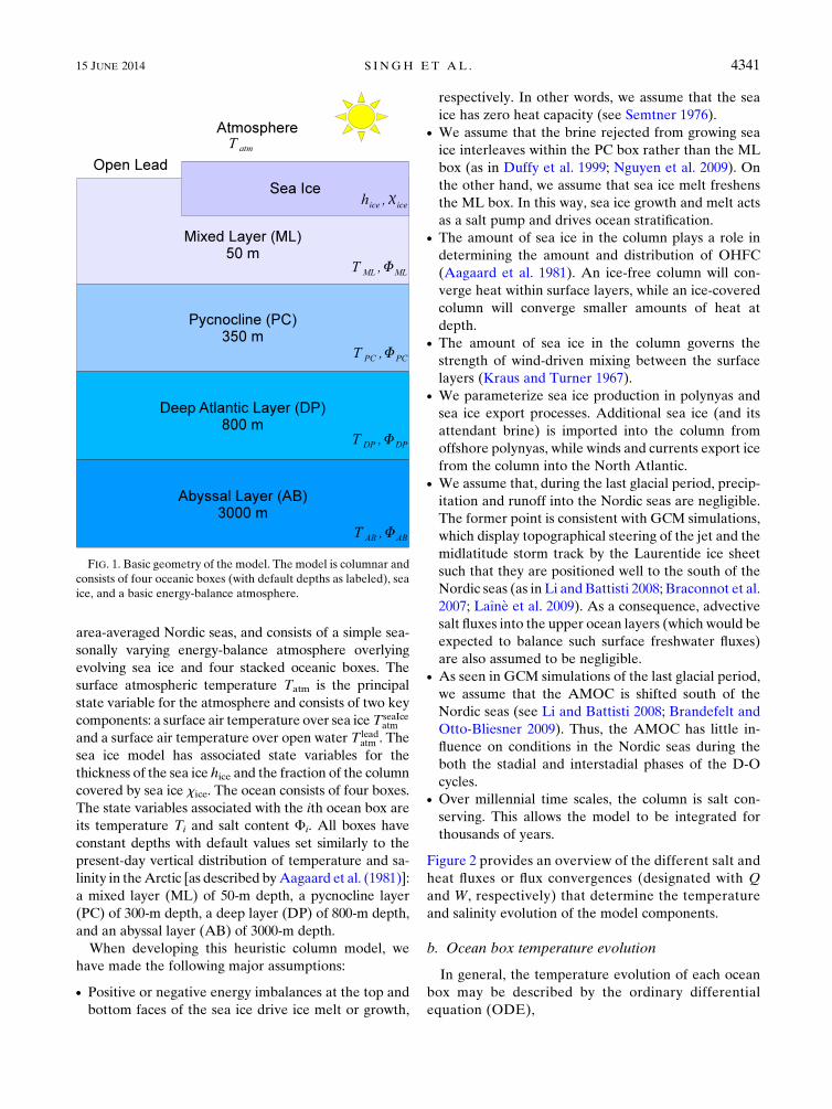
area-averaged Nordic seas, and consists of a simple sea-

sonally varying energy-balance atmosphere overlying

evolving sea ice and four stacked oceanic boxes. The

surface atmospheric temperature Tatm is the principal

state variable for the atmosphere and consists of two key

components: a surface air temperature over sea iceTseaIceatm

and a surface air temperature over open water T leadatm . The

sea ice model has associated state variables for the

thickness of the sea ice hice and the fraction of the column

covered by sea ice xice. The ocean consists of four boxes.

The state variables associated with the ith ocean box are

its temperature Ti and salt content Fi. All boxes have

constant depths with default values set similarly to the

present-day vertical distribution of temperature and sa-

linity in theArctic [as described byAagaard et al. (1981)]:

a mixed layer (ML) of 50-m depth, a pycnocline layer

(PC) of 300-m depth, a deep layer (DP) of 800-m depth,

and an abyssal layer (AB) of 3000-m depth.

When developing this heuristic column model, we

have made the following major assumptions:

d Positive or negative energy imbalances at the top and

bottom faces of the sea ice drive ice melt or growth,

respectively. In other words, we assume that the sea

ice has zero heat capacity (see Semtner 1976).d We assume that the brine rejected from growing sea

ice interleaves within the PC box rather than the ML

box (as in Duffy et al. 1999; Nguyen et al. 2009). On

the other hand, we assume that sea ice melt freshens

the ML box. In this way, sea ice growth and melt acts

as a salt pump and drives ocean stratification.d The amount of sea ice in the column plays a role in

determining the amount and distribution of OHFC

(Aagaard et al. 1981). An ice-free column will con-

verge heat within surface layers, while an ice-covered

column will converge smaller amounts of heat at

depth.d The amount of sea ice in the column governs the

strength of wind-driven mixing between the surface

layers (Kraus and Turner 1967).d We parameterize sea ice production in polynyas and

sea ice export processes. Additional sea ice (and its

attendant brine) is imported into the column from

offshore polynyas, while winds and currents export ice

from the column into the North Atlantic.d We assume that, during the last glacial period, precip-

itation and runoff into the Nordic seas are negligible.

The former point is consistent with GCM simulations,

which display topographical steering of the jet and the

midlatitude storm track by the Laurentide ice sheet

such that they are positioned well to the south of the

Nordic seas (as in Li andBattisti 2008; Braconnot et al.

2007; Laın�e et al. 2009). As a consequence, advective

salt fluxes into the upper ocean layers (which would be

expected to balance such surface freshwater fluxes)

are also assumed to be negligible.d As seen in GCM simulations of the last glacial period,

we assume that the AMOC is shifted south of the

Nordic seas (see Li and Battisti 2008; Brandefelt and

Otto-Bliesner 2009). Thus, the AMOC has little in-

fluence on conditions in the Nordic seas during the

both the stadial and interstadial phases of the D-O

cycles.d Over millennial time scales, the column is salt con-

serving. This allows the model to be integrated for

thousands of years.

Figure 2 provides an overview of the different salt and

heat fluxes or flux convergences (designated with Q

and W, respectively) that determine the temperature

and salinity evolution of the model components.

b. Ocean box temperature evolution

In general, the temperature evolution of each ocean

box may be described by the ordinary differential

equation (ODE),

FIG. 1. Basic geometry of the model. The model is columnar and

consists of four oceanic boxes (with default depths as labeled), sea

ice, and a basic energy-balance atmosphere.

15 JUNE 2014 S I NGH ET AL . 4341

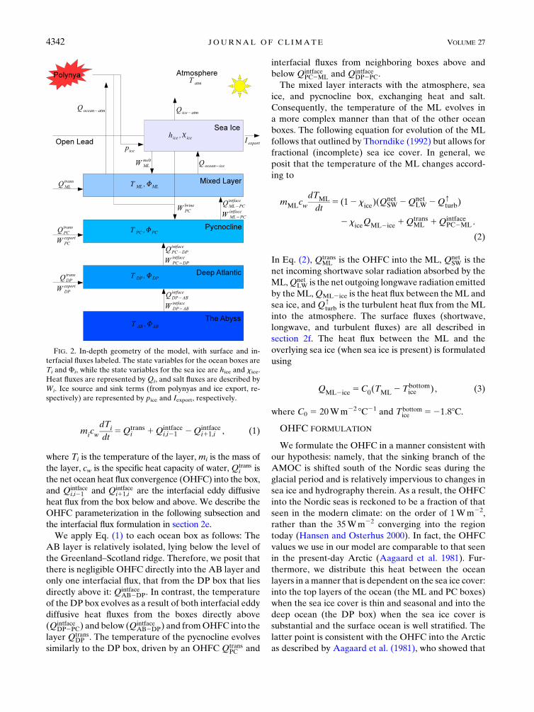
micwdTi

dt5Qtrans

i 1Qintfacei,i21 2Qintface

i11,i , (1)

where Ti is the temperature of the layer,mi is the mass of

the layer, cw is the specific heat capacity of water,Qtransi is

the net ocean heat flux convergence (OHFC) into the box,

and Qintfacei,i21 and Qintface

i11,i are the interfacial eddy diffusive

heat flux from the box below and above. We describe the

OHFC parameterization in the following subsection and

the interfacial flux formulation in section 2e.

We apply Eq. (1) to each ocean box as follows: The

AB layer is relatively isolated, lying below the level of

the Greenland–Scotland ridge. Therefore, we posit that

there is negligible OHFC directly into the AB layer and

only one interfacial flux, that from the DP box that lies

directly above it: QintfaceAB2DP. In contrast, the temperature

of the DP box evolves as a result of both interfacial eddy

diffusive heat fluxes from the boxes directly above

(QintfaceDP2PC) and below (Qintface

AB2DP) and fromOHFC into the

layer QtransDP . The temperature of the pycnocline evolves

similarly to the DP box, driven by an OHFC QtransPC and

interfacial fluxes from neighboring boxes above and

below QintfacePC2ML and Qintface

DP2PC.

The mixed layer interacts with the atmosphere, sea

ice, and pycnocline box, exchanging heat and salt.

Consequently, the temperature of the ML evolves in

a more complex manner than that of the other ocean

boxes. The following equation for evolution of the ML

follows that outlined by Thorndike (1992) but allows for

fractional (incomplete) sea ice cover. In general, we

posit that the temperature of the ML changes accord-

ing to

mMLcwdTML

dt5 (12 xice)(Q

netSW 2Qnet

LW 2Q[turb)

2 xiceQML2ice1QtransML 1Qintface

PC2ML .

(2)

In Eq. (2), QtransML is the OHFC into the ML, Qnet

SW is the

net incoming shortwave solar radiation absorbed by the

ML,QnetLW is the net outgoing longwave radiation emitted

by theML,QML2ice is the heat flux between theML and

sea ice, andQ[turb is the turbulent heat flux from the ML

into the atmosphere. The surface fluxes (shortwave,

longwave, and turbulent fluxes) are all described in

section 2f. The heat flux between the ML and the

overlying sea ice (when sea ice is present) is formulated

using

QML2ice 5C0(TML 2Tbottomice ) , (3)

where C0 5 20Wm22 8C21 and Tbottomice 521:88C.

OHFC FORMULATION

We formulate the OHFC in a manner consistent with

our hypothesis: namely, that the sinking branch of the

AMOC is shifted south of the Nordic seas during the

glacial period and is relatively impervious to changes in

sea ice and hydrography therein. As a result, the OHFC

into the Nordic seas is reckoned to be a fraction of that

seen in the modern climate: on the order of 1Wm22,

rather than the 35Wm22 converging into the region

today (Hansen and Osterhus 2000). In fact, the OHFC

values we use in our model are comparable to that seen

in the present-day Arctic (Aagaard et al. 1981). Fur-

thermore, we distribute this heat between the ocean

layers in amanner that is dependent on the sea ice cover:

into the top layers of the ocean (the ML and PC boxes)

when the sea ice cover is thin and seasonal and into the

deep ocean (the DP box) when the sea ice cover is

substantial and the surface ocean is well stratified. The

latter point is consistent with the OHFC into the Arctic

as described by Aagaard et al. (1981), who showed that

FIG. 2. In-depth geometry of the model, with surface and in-

terfacial fluxes labeled. The state variables for the ocean boxes are

Ti and Fi, while the state variables for the sea ice are hice and xice.

Heat fluxes are represented by Qi, and salt fluxes are described by

Wi. Ice source and sink terms (from polynyas and ice export, re-

spectively) are represented by pice and Iexport, respectively.


warm, salty water transported from the Atlantic into the

Arctic will subduct beneath a cold halocline (as posited

to exist in the Nordic seas during stadial conditions,

when sea ice cover is perpetual) and enter the water

column at great depth (.500m).

Table 1 describes the notation for and typical values of

the OHFC into the model ocean boxes. The vertical

distribution of OHFC depends strongly on xice, the sea

ice fraction in the column, while the magnitude of the

OHFC depends only mildly on this quantity. In partic-

ular, we parameterize the OHFC into the DP layer as

QtransDP 5 xiceQ

Icetot , whereQIce

tot 5 0.5Wm22 and xice is the

sea ice fraction. For the PC layer,

QtransPC 5 (12 xice)

1

3QNoIce

tot , (4)

whereQNoIcetot is the total OHFC when the system is in an

ice-free state, reckoned to be 3Wm22 in the control

simulation. Analogous to the PC, the OHFC into the

ML is nil when the column is ice covered but is nonzero

when the column is ice free,

QtransML 5 (12 xice)

2

3QNoIce

tot . (5)

In Eqs. (4) and (5), the factors of 1/3 and 2/3 permit us to

partition the OHFC between the PC and ML boxes,

respectively, allowing for the heating to be surface

weighted such that a greater fraction converges in the

ML box than in the PC box.

c. Sea ice evolution

Wemodel the seasonal growth and melt of the sea ice

after Thorndike (1992). When sea ice cover is complete

(there is no open water), the sea ice evolves according to

riceLf

dVice

dt52QML2ice 1Qnet

LW 2QnetSW

1 riceLf

dpicedt

2 Iexport , (6)

where rice is the density of sea ice, Lf is the heat of fusion

for seawater,Vice is the volume of the ice,QML2ice is the

heat flux into the ice from theML [formulated according

to Eq. (3)], QnetSW is the net shortwave radiation incident

on the ice, QnetLW is the net longwave radiation at the top

surface of the ice, dpice/dt is a sea ice source term to

model distally formed sea ice advected into the column

from polynyas, and Iexport is a sea ice sink term to model

ice export from the Nordic seas. The formulation of the

shortwave, longwave, and atmospheric heat transport

fluxes in Eq. (6) will be described in section 2f. We de-

scribe the polynya source and ice export sink terms in

the following two paragraphs.

As described in Martin et al. (1998) and Cavalieri and

Martin (1994), we posit that latent heat polynyas driven

by katabatic winds blowing off the Fennoscandian ice

sheet (FSIS) were responsible for the production of sea

ice along the FSIS during the last glacial. This ice is then

swept into the wider Nordic seas by winds and currents,

accelerating ice growth beyond that expected from local

conditions. In ourmodel, we setÐ(dpice/dt) dt5 1:0mper

cold season, provided that the sea ice thickness within the

column is greater than or equal to 1.0m. When hice is less

than 1.0m, there is no extra polynya ice added to the

column. Note that brine rejected from polynya ice is also

assumed to interleave into the PC layer, just like brine

rejected from sea ice formed in situ.

We hypothesize that some of the sea ice formedwithin

the Nordic seas during the last glacial cycle was exported

from theNordic seas into theNorthAtlantic. To account

for the export of sea ice from the column, we formulate

a yearly cumulative export term Iexport as the integrated

sum of the ice grown within the column per year, mul-

tiplied by an ice export factor Cr,

Iexport 5Cr

ð1yr

dV

growthice

dt

!dt . (7)

Each year, we remove a quantity of ice from the column

Iexport, which corresponds to the yearly export of

(100Cr)% of the ice formed within the column per

annum. We use Cr 5 0.05, corresponding to the export

of 5.0% of the ice formed within the Nordic seas per

year.

TABLE 1. Values ofQtransX , the OHFC, into the model ocean boxes. Both the general formulation and the specific formulation (during

ice-covered and ice-free conditions) are shown.

Ocean box General xice 5 1 (ice present) xice 5 0 (ice free)

ML: QtransML

2/3QNoIcetot (12 xice) 0 2.0Wm22

PC: QtransPC

1/3QNoIcetot (12 xice) 0 1.0Wm22

DP: QtransDP QIce

totxice 0.5Wm22 0

AB 0 0 0

Total Sum of above QIcetot 5 0:5Wm22 QNoIce

tot 5 3:0Wm22

15 JUNE 2014 S I NGH ET AL . 4343

When sea ice cover is incomplete and open water is

present, energy conservation requires that the sea ice

evolve according to

riceLf

dVice

dt5 xice(Q

netLW2Qnet

SW 2QML2ice)

1 riceLf

dpicedt

2 Iexport , (8)

where xice is the fraction of the column covered by sea

ice. In general, the volume of sea ice present is related to

the ice thickness hice and ice area by Vice 5 hicexice. The

ice fraction xice may be diagnosed for a given hice using

the following formulation:

xice 5

0 for hice 5 0m

2hice for hice 2 (0, 0:5]m

1 for hice . 0:5m

.

8><>: (9)

Equation (8) reduces to Eq. (6) when hice . 0.5m,

meaning that xice 5 1.

d. Ocean salinity

We formulate the salinity evolution of the different

components of the system using an equation for salt

content (in units of grams salt) within the ith layer,

dFi

dt5Wintface

i,i21 2W intfacei11,i 1Wx

i , (10)

where W intfacei,i21 and W intface

i11,i refer to the interfacial salt

fluxes with layers below and above and Wxi is a term

representing horizontal or vertical advective fluxes of

salt due to sea ice growth and melt, as well as transport

processes (which we will detail further below). The sa-

linity may be derived from the salt content using

Si 5Fi/(rihi), where hi is the depth of the ith layer and

ri is its density.We compute the density of the box in this

and all subsequent calculations using the full equation of

state for seawater (from Gill 1982).

The salt content of the ML evolves due an interfacial

salt flux from the PC W intfaceML2PC and a negative salt flux

from sea icemeltWmeltML . Given a particular rate of sea ice

melt dVice/dt and assuming (for simplicity) that sea ice

has no salt content, the meltwater flux may be formu-

lated as

WmeltML 5 rice

S0ML�12

S0ML

1000

� dVmeltice

dt, (11)

where S0ML is a reference salinity (taken to be the initial

salinity of the mixed layer). We derive Eq. (11) from the

assumption that the mass of ice melted per unit time

results in amass flux of salt-free water (equal to themass

flux of the melted ice) added to the mixed layer, thereby

lowering its total salt content. Note that we use the

reference salinity S0ML to estimate the negative mass flux

of salt associated with this sea ice melt rate. This allows

the column to be salt conserving over time scales ex-

ceeding 1 yr, since the negative salt flux associated with

sea ice melt is balanced by a positive salt flux into the

pycnocline because of brine rejected when the sea ice

was formed.

The salt content of the PC evolves because of brine

rejected as a result of sea ice formation WbrinePC ; a fresh-

water recirculation flux resulting from ice exportWexportPC,DP

(see the following paragraph for a description of this

term); and interfacial fluxes from the neighboring ML

and DP boxes W intfaceML2PC and W intface

PC2DP, respectively. As

described in coupled modeling studies by Duffy et al.

(1999) andNguyen et al. (2009), we formulate ourmodel

so that all the brine rejected from sea ice formation

(both within the column and in polynyas) is assumed to

sink to the depth of the pycnocline and interleave

therein, thereby enhancing the cold halocline. We for-

mulate this salt flux into the pycnocline analogously to

the negative salt flux into the ML resulting from sea ice

melt, Eq. (11),

WbrinePC 5 rice

S0ML�12

S0ML

1000

� dVgrowice

dt. (12)

The salt content of the DP box evolves via interfacial

fluxes from the neighboring boxes PC and AB boxes

(W intfacePC2DP and W intface

DP2AB, respectively), as well as a nega-

tive salt flux arising from ice export from the column

WexportPC,DP. We model this ice export term as follows:

ð1yr

WexportPC,DP dt5 rice

S0ML�12

S0ML

1000

� Iexport . (13)

The rationale behind this term is that ice exported from

the Nordic seas into the North Atlantic, where it melts

and is entrained into the sinking branch of the AMOC

south of the Nordic seas, creating fresher water below

that subsequently recirculates back into the Nordic seas

at the level of the PC and DP layers. The ice export sink

term causes the column to salinize over long time scales;

including this freshening term allows the column to be

salt conserving. The fraction of the negative salt flux

added to the PC andDP is FPC and 12 FPC, respectively,

where the default value of FPC is taken to be 0.8. Finally,


the AB box evolves solely through an interfacial diffu-

sive salt flux with the DP box W intfaceDP2AB.

e. Formulation of interfacial fluxes and convectivemixing

We parameterize vertical mixing processes between

ocean boxes as follows: When the system is stably

stratified, the density of the underlying box j is greater

than that of the overlying box i: rj . ri. In this case,

mixing between boxes will be either eddy driven or

diffusive, depending on the depth of the boxes involved.

In general, interfacial mixing between the ith and jth box

results in the following heat and salt fluxes:

Qintfacei,j 5

2KTi,jcw(riTi 2 rjTj)

hi 1 hjand (14)

Wintfacei,j 5

2KSi,j(riSi2 rjSj)

hi 1 hj, (15)

where hi is the depth of the ith box andKXi,j is the mixing

coefficient for property X across the interface between

boxes i and j. The assumption behind this formulation is

that mixing across interfaces results in the exchange of

equal volumes of seawater between boxes: water that

carries the temperature and salinity properties of its

parent box into its new residence, thereby changing the

state variables of both boxes.

We have assigned the coefficients of vertical mixing

KTi,j and KS

i,j between each set of boxes based on the

depth of the layers in question. As described in Wunsch

and Ferrari (2004) and Gargett (1984), turbulent eddies

are the dominant mode of vertical mixing within the top

200m of the ocean. Such eddies mix heat and salt in the

upper ocean, with the magnitude of the mixing co-

efficient on the order of 1 3 1024m2 s21 (as in Gargett

1984). In such a case, we expect thatKT5KS, since both

properties will be transported equally by eddy-driven

mixing processes. We posit mixing at the interface be-

tween the ML and PC boxes is eddy driven, so

KTML2PC 5KS

ML2PC 5O(1024)m2 s21.

As described in Kraus and Turner (1967), the extent

of mixing in the upper layer of the ocean is wind driven

and therefore moderated by the fraction of ocean sur-

face covered with sea ice. Therefore, we assign specific

values toKT,SML2PC based on the extent of sea ice cover, as

follows:

KT,SML2PC 5 xiceK

T,S2IceML2PC1 (12 xice)K

T,S2NoIceML2PC . (16)

In Eq. (16), we have assignedKT,S2IceML2PC 5 13 1024 m2 s21

and KT ,S2NoIceML2PC 5 63 1024 m2 s21. Equation (16) posits

a larger amount of upper-ocean mixing when xice , 1

and a smaller amount of upper-ocean mixing when

xice ’ 1.

On the other hand, vertical mixing at depths greater

than 400m is dominated by diffusive processes, as de-

scribed by Huppert and Turner (1981). In this realm,

heat and salt diffuse at separate rates, based on their

molecular diffusivity. At a given depth, the molecular

diffusivity of heat exceeds the molecular diffusivity of

salt by a factor of at least 10, giving KT 5 10KS. Fur-

thermore, we expect that the magnitude of mixing be-

tween the PC and DP boxes is larger than that between

the DP and AB boxes, because of the greater depth of

the latter. Therefore, we have set the remainder of the

vertical eddy diffusive coefficients as follows: KTPC2DP 5

1025 m2 s21,KSPC2DP 5 1026 m2 s21,KT

DP2AB 5 1027 m2 s21,

and KSDP2AB5 1028 m2 s21.

When the density of an overlying box exceeds that of

an underlying box, we assume mixing is done by con-

vection. In this case, we completely mix the temperature

and salinity in the two layers.

f. Formulation of surface conditions, processes, andfluxes

We diagnose the surface air temperature as an aver-

age of the surface temperature over open waterTML and

the surface air temperature over sea iceTtopice weighted by

the fraction of sea ice cover in the column,

Tatm5 xiceTtopice 1 (12xice)TML . (17)

We describe the calculation of Ttopice , the temperature at

the top of the ice, in Eq. (22).

We formulate the surface processes included inEq. (2),

the equation governing the evolution of the ML box,

and Eq. (6), the equation governing the evolution of the

sea ice, as follows: First, following Thorndike (1992) we

assign the mean shortwave flux reaching the surface

during the warm half of the year as FSW ’ 200Wm22

and as 0Wm22 during the cold half. Taking into account

the albedo ai of the surface receiving the radiation, we

obtain the following formulation for the net shortwave

fluxes:

QnetSW 5

8<:

(12aice)FSW over sea ice in summer

(12aocn)FSW over open ocean in summer

0 over sea ice or open ocean in winter

. (18)

15 JUNE 2014 S I NGH ET AL . 4345

Since aice ’ 0.6 and aocn ’ 0.1, the net shortwave flux

absorbed during the warm half of the year by the ML

and sea ice are 180 and 80Wm22, respectively.

Next, the net longwave flux in Eqs. (2) and (6) can be

approximated as per Thorndike (1992) as follows:

QnetLW’

A1BTsurf

n2D/2 , (19)

assuming the surface temperature (ocean mixed layer,

sea ice, or both) is in equilibrium with the overlying

atmosphere, where Tsurf is the temperature of the

surface; the constants A and B are equal to 320Wm22

and 4.6Wm22 8C21, respectively; and D, the atmo-

spheric heat transport flux convergence, is taken to be

90Wm22. The quantity n refers to the optical depth of

the atmosphere and may be used to approximate the

effects of reabsorption and reemission between the

surface and atmosphere. As in Thorndike (1992), n

depends on season and sea ice cover. Thus, Eq. (19)

becomes

QnetLW5

8>>>><>>>>:

(A1BTML)/ns 2D/2 over open ocean, summer

(A1BTML)/nw 2D/2 over open ocean, winter

A/ns 2D/2 over sea ice, summer

(A1BTtopice )/nw 2D/2 over sea ice, winter

, (20)

where nw 5 2.5 during the cold half of the year for both

ice-covered and ice-free periods, ns5 2.8 during the warm

half of the year during ice-covered periods, and ns 5 2.9

during the warm half of the year during ice-free periods.

During the warm half of the year, we assume Ttopice 5 08C.

The temperature at the top of the ice during the cold

half of the year is found from equating the energy fluxes

at the top surface of the ice QnetLW 5Q[

cond, where Q[cond

is the conductive heat flux through the ice. From

Thorndike (1992),

Q[cond 5

k(Ttopice 2Tbot

ice )

hice. (21)

Substituting Eqs. (21) and (20) into QnetLW 5Q[

cond and

solving for Ttopice during the cold half of the year gives

Ttopice 5

1

B/nwinter1 k/hice

kTbot

ice

hice2

A

nwinter1

D

2

!. (22)

Finally, we approximate the atmosphere to ocean tur-

bulent heat flux Q[turb using a bulk formulation (as in

Peixoto and Oort 1992),Q[turb 5BT(TML 2Tref), where

BT ’ 5.0Wm22 8C21 and Tref is the minimum temper-

ature the ML box may attain (21.88C).

g. Numerical methods

We used the forward Euler method to discretize the

time derivatives found in the model equations. We in-

tegrated the model asynchronously in order to accom-

modate the very different time scales involved in the

components. Surface processes, including those involv-

ing the atmosphere, mixed layer, and sea ice, evolve

rapidly on scales shorter than a season (as described in

Thorndike 1992). For these components, we used a time

step of Dt 5 1/200 yr. Middle and deep oceanic pro-

cesses, however, have much slower time scales (Wunsch

and Ferrari 2004), allowing integration of these com-

ponents with a time step of Dt 5 1/20 yr.

3. Model results

The model, as detailed in previous sections, replicates

many of the essential features of the D-O cycles (see

Fig. 3 for a 6000-yr integration of the standard model).

We begin by considering the stadial phase in the standard

model output, which is approximately 1100 yr long with

perennial sea ice cover in the Nordic seas. Seasonally, the

sea ice has a maximal thickness of approximately 3.0m at

the end of winter and a minimum thickness of 2.3m at the

end of summer (Fig. 4).With this perennial sea ice, surface

air temperature is approximately 2228C during the cold

season, for an average annual temperature of 2118C(Fig. 5). The temperatures in the upper-ocean boxes are

also close to the freezing point, TML ’ 228C and TPC ’218C. The temperature in the PC box, however, increases

slightly over the course of the stadial period because of

diffusive heat fluxes between the PC and DP boxes (not

shown). The temperature in the DP box rises substan-

tially, increasing from approximately 4.48 to 4.98Cover the

1100 yr of the stadial period (Fig. 6). Though the tem-

peratures of the ML and PC are close throughout the

stadial phase, their salinities are very different (Fig. 7).

During the stadial, SPC increases from 34.2 to 34.9psu,

while SML increases from 33.5 to 34.0 psu (Fig. 7), resulting

in extremely strong density stratification in the upper

ocean throughout this period (Fig. 8). Such a stable cold

halocline is similar to that seen today in the Arctic Ocean

under its perennial sea ice cover (Aagaard et al. 1981).


Finally, the salinity of the DP decreases slowly, from 32.8

to 32.2 psu, over the course of the stadial period (Fig. 7)

because of sea ice exported into the Atlantic: sea ice ex-

port causes freshening of theAtlantic water that circulates

in this layer (as diffusive exchange with the PC box would

increase salinity and exchange with the AB box is negli-

gible). Indeed, making the export coefficient Cr zero re-

sults in little net freshening of the DP layer (not shown).

The transition from the stadial to interstadial period is

extremely rapid (as seen in Figs. 6 and 7), occurring over

a brief 3-yr span (not shown). Convective overturning of

the PC and DP boxes initiates the transition to the in-

terstadial period. This overturning event is caused by

a combination of factors, which all conspire to decrease

rDP and increase rPC, thereby equalizing their densities

and initiating convection (Figs. 8 and 9): the increase in

the temperature of the DP layer (due to weak OHFC

into the DP box), the decrease in the salinity of the DP

layer, and the increase in the salinity of the PC layer

(due to brine rejection from sea ice formation and sub-

sequent export). The overturning of the PC and DP

boxes quickly raises the temperature of the PC box to

about 38C at the start of the interstadial (Fig. 5). Next,

the large temperature gradient between the ML and PC

drives an upward flux of heat into the ML box through

eddy-driven vertical mixing, thereby increasing the

temperature of the mixed layer, increasing the ice–

ocean conductive heat flux by several orders of magni-

tude, and allowing the perennial sea ice cover to melt

rapidly, giving way to seasonal sea ice (Figs. 4 and 5).

The overturning event also causes the salinities of the

PC and DP boxes to equalize. The salinity of the mixed

layer decreases rapidly because of abrupt sea ice melt

during the stadial to interstadial transition, hitting a low

point of SML ’ 31.8 psu (Fig. 4).

The interstadial phase is approximately 150 yr in

length. The model output, particularly from Figs. 4 and

5, suggests that the interstadial period has several dif-

ferent phases. The first phase corresponds to the rapid

decay of the PC box temperature from its maximum

value of 38C to about 28C, a process that takes approx-

imately 20 yr. After an initial adjustment process (,5 yr)

in which the temperature of the ML box increases from

21.88 to 38C (annually averaged), the ML box evolves

similarly to the PC box, though it experiences sub-

stantial seasonal cycling because of its interaction with

FIG. 3. Results for (top) atmosphere and ocean temperature, (middle) sea ice thickness,

and (bottom) ocean salinity from 6000 yr of output from the model with default parameter

values. Except for the atmospheric temperature, the model output, which reports all state

variables biannually (once at the end of the warm season and again at the end of the cold

season), has been smoothed with a 5-yr running-mean filter; the atmospheric temperature

has been smoothed with a 25-yr running-mean filter to mirror the resolution of the d18O ice

core proxy used to infer Greenland surface temperature. In (top), the temperature of the

PC box is not shown; at the scale of this figure, the temperatures of the ML and PC are

indistinguishable.

15 JUNE 2014 S I NGH ET AL . 4347

the atmosphere and sea ice (see Figs. 5 and 6). Following

this initial rapid decay, we also discern that there is

a phase of slow decay (with a long time scale of several

hundred years), in which the maximum thickness of the

sea ice increases gradually (from 2.2 to 2.5m; Fig. 4) and

the temperatures of the ML and PC boxes decay slowly

(from 1.58 to 1.28C in both theML and PC boxes; Fig. 6).

The salinities of the PC and ML boxes, which briefly

equalized at the beginning of the interstadial period

because of rapid sea ice melt and eddy-driven vertical

exchange, diverge during the interstadial, and the ML

and PC layers begin to restratify: as themaximumwinter

thickness of the sea ice increases throughout this period,

this results in a net flux of brine into the PC box, thereby

increasing its salinity and density (Figs. 7–9).

The transition back to the stadial phase, in which the

system has year-round sea ice cover, is slower than the

abrupt transition to the interstadial phase. There ap-

pear to be two time scales associated with this transition.

There is a short time scale of approximately 10–20yr as-

sociated with the summer temperature of the ML

box returning to below 21.08C, the sea ice thickness

returning to its stadial range, and the end-of-winter at-

mospheric temperature returning to 2228C (Figs. 4 and

6). There is also a longer time scale of approximately

50 yr associated with the time required for the pycno-

cline temperature and the end-of-summer ice thickness

to relax to their averaged stadial values, 21.08C and

2.3m, respectively.

Figure 10 provides a pictorial summary of the major

processes that characterize the stadial and interstadial

phases in the model. The difference between the fluxes

in the two phases results from major differences in the

sea ice cover: a substantial, perennial sea ice cover

during the stadial period and a thinner, seasonal sea ice

cover during the interstadial. During the stadial phase,

a robust perennial ice cover allows for vigorous ice ex-

port and accompanying freshwater recirculation into the

DP layer; during the interstadial, both export and re-

circulation are comparatively weaker as there is less ice

to export. During the interstadial phase, the column

spends a significant amount of time in an ice-free state,

FIG. 4. Unsmoothedmodel output showing the seasonal evolution of (top) sea ice thickness and (bottom) salinities

of the ML and PC ocean boxes during a typical interstadial event. This model output is biannual, with all state

variables reported at the end of the winter (cold) season and at the end of the summer (warm) season.


and the resulting wind-driven mixing between the ML

and PC boxes is strong compared to that during the

stadial phase. The perennial sea ice cover during the

stadial is augmented by polynya ice, which is imported

into the column (with its accompanying brine), while the

interstadial column, which only possesses a seasonal sea

ice cover, does not receive extra ice and brine input from

polynyas. During the interstadial phase, large amounts

of sea ice grow and melt annually with the seasonal cy-

cle, whereas during the stadial phase this seasonal cycle

in sea ice cover is much smaller. As a consequence, the

input of freshwater into the ML box from melt and the

PC box from brine rejection is much larger during the in-

terstadial than the stadial. Finally, as we have summarized

in Table 1, the OHFC during the stadial period is into

the DP box, while the OHFC during the interstadial is

shared by the ML and PC boxes.

4. Sensitivity studies

a. OHFC parameters

Figure 11 provides an overview of the sensitivity of the

stadial and interstadial time scales to changes in the

OHFC parameters,QNoIcetot andQIce

tot . First and foremost,

we see that for the model to support D-O-like oscilla-

tions, the net heat transport into the Nordic seas must be

small throughout the cycle, comparable to that seen

today in the Arctic, and a small fraction of that into the

Nordic seas today. This finding is consistent with our

supposition that the sinking branch of the AMOC ter-

minates south of the Nordic seas throughout the glacial

period and that the position of this sinking branch is

relatively insensitive to the state of the Nordic seas.

In general, we see that the model produces robust

oscillations over a reasonable range of values of these

OHFC parameters and that this range is between one to

two orders of magnitude less than the OHFC into the

Nordic seas today. In particular, we see that oscillations

reminiscent of D-O events (with interstadial phases

greater than 75 yr in length andwith total cycles between

1000 and 1500 yr in length) occur over a 50% change in

QNoIcetot and a 40% change in QIce

tot .

The ranges ofQNoIcetot andQIce

tot in Fig. 11 were chosen to

highlight the central region about which physically rel-

evant oscillations exist, given the default parameter

values listed in Table 2. We note that oscillations still

occur for QIcetot , 0:4Wm22 and QNoIce

tot , 0:75Wm22

(even though the length of the interstadial phase is less

than 75 yr), suggesting that the oscillations themselves

are robust to changes in OHFC values; the length of the

interstadial phase, however, is more sensitive to such

changes.

To produce Fig. 11, we have defined the onset of the

interstadial phase as when the PC andDP boxes become

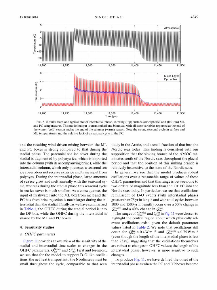
FIG. 5. Results from one typical model interstadial phase, showing (top) surface atmospheric, and (bottom) ML

and PC temperatures. This model output is unsmoothed and biannual, with all state variables reported at the end of

the winter (cold) season and at the end of the summer (warm) season. Note the strong seasonal cycle in surface and

ML temperatures and the relative lack of a seasonal cycle in the PC.

15 JUNE 2014 S I NGH ET AL . 4349

buoyantly unstable and overturn (as described in section

3); the end of the interstadial phase (and beginning of

the stadial phase) is defined to be when the temperature

of the PC box has relaxed to 0.18C of its stadial value;

and the time required for a single cycle (stadial plus

interstadial phases) is taken to be the time between

overturning events. It is possible for the interstadial

phase to go on forever (hatched regions of Fig. 11) when

the ML and PC boxes cannot rid themselves of excess

heat, a requirement if perennial sea ice is to reform.

Whether the model reforms perennial sea ice depends

on several bifurcation parameters. We will carefully

consider these parameters and their implications in

a forthcoming paper.

From examining Fig. 11, we see that the total OHFC

when ice is present (QIcetot ) affects the length of the sta-

dial, and hence how long it takes for the ocean column

to become convectively unstable and overturn. Such

a process brings deep ocean heat up to the surface and

melts the ice, initiating the interstadial phase. On the

other hand, we see that the total OHFC when ice is

absent (QNoIcetot ) affects the interstadial time scale, the

time required for the column to cool and support the

regrowth of perennial sea ice. We will further describe

the relationship of these and other parameters to the

lengths of the interstadial and stadial phases in section 4e.

b. Vertical distribution of OHFC during ice-freeconditions

In our control simulation, we have apportioned QNoIcetot ,

the total (vertically integrated) OHFC during ice-free

conditions, as follows: two-thirds of the total heat flux

enters the ML box and one-third of the total heat flux

enters the PC box. The sensitivity to the choice of how

we distribute the OHFC vertically is tested in two al-

ternate model configurations: one with a larger pro-

portion of the ice-free OHFC concentrated in the ML

box and less in the PC box and one with a smaller pro-

portion of ice-free OHFC concentrated in the ML box

and more in the PC.

Table 3 shows the sensitivity of the model to such

changes in the distribution of QNoIcetot . Here, we present

the time scales produced by the model in the case where

we have modified the value of BT to 5.5Wm22 8C21

(from 5.0Wm22 8C21) and have left the values of other

control parameters unchanged. We record the length of

the interstadial phase and cycle duration when the ratio

of OHFC into theML and PC boxes are shifted from 2:1

(as in the control) to 1:1 (more of total OHFC into the

PC box) and 3:1 (more of total OHFC into theML box).

We find that, while the lengths of the stadial and inter-

stadial phases aremodified by this choice, the fundamental

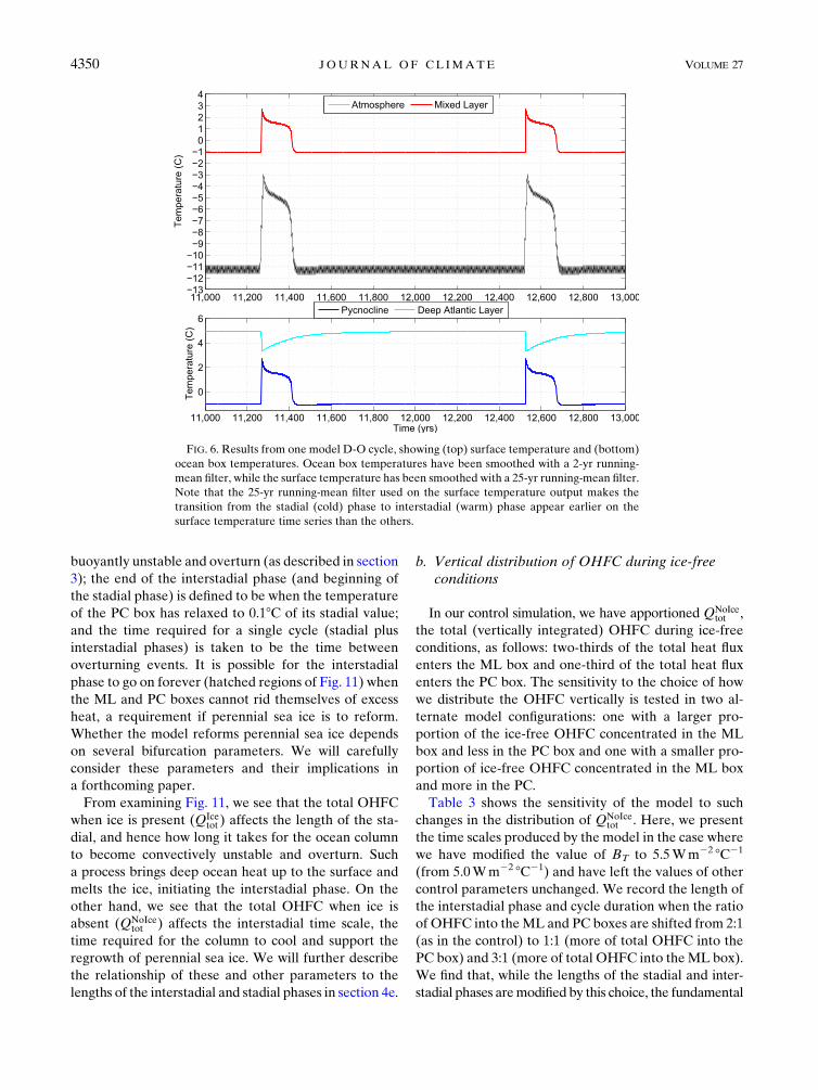
FIG. 6. Results from one model D-O cycle, showing (top) surface temperature and (bottom)

ocean box temperatures. Ocean box temperatures have been smoothed with a 2-yr running-

mean filter, while the surface temperature has been smoothed with a 25-yr running-mean filter.

Note that the 25-yr running-mean filter used on the surface temperature output makes the

transition from the stadial (cold) phase to interstadial (warm) phase appear earlier on the

surface temperature time series than the others.


behavior of the model (oscillations between stadial and

interstadial phases on a millennial time scale) does not

change appreciably (the changes in the length of the

stadial and interstadial phases in the 3:1 and 1:1 cases are

within 5% and 60%, respectively, of those in the 2:1

control case). Therefore, we conclude that the model is

robust to changes in the vertical distribution of OHFC

during ice-free conditions.

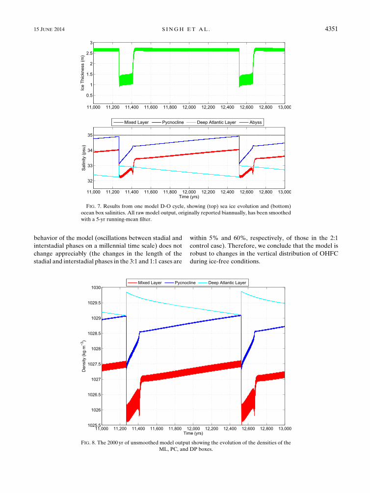
FIG. 7. Results from one model D-O cycle, showing (top) sea ice evolution and (bottom)

ocean box salinities. All raw model output, originally reported biannually, has been smoothed

with a 5-yr running-mean filter.

FIG. 8. The 2000 yr of unsmoothed model output showing the evolution of the densities of the

ML, PC, and DP boxes.

15 JUNE 2014 S I NGH ET AL . 4351

c. Temporal variability in ocean and atmosphericheat flux convergence

1) OHFC

Observational studies show that the OHFC into the

Nordic seas today is variable on interannual time scales

on the order of 5–10 yr (see Hatun et al. 2005). Although

the North Atlantic gyre is displaced southward in the

glacial climate due to changes in the wind stress curl

(see, e.g., Li and Battisti 2008; Braconnot et al. 2007;

Laın�e et al. 2009), we explore the impact of general

stochastic variability in the OHFC on the modeled D-O

cycles by adding a red noise component to QNoIcetot ,

(QNoIcetot )i 5 l(QNoIce

tot )0 1 (12 l)(QNoIcetot )i211 � , (23)

where l is Dt over the time scale over which OHFC is

said to be variable (for Dt 5 1 yr, realistic modern vari-

ability in the OHFC is simulated when l 5 1/5–1/10)

and � is the appropriately scaled white noise process.

Substituting such a process for our static QNoIcetot with

other parameters held at their control values results in

an increase in the length of the interstadial phase, from

150 yr to nearly 180 yr. Furthermore, we find the phase

space that supports physically relevant oscillations (as

defined in section 4a above) is widened in the QNoIcetot

dimension by approximately 10% with such a modifica-

tion (not shown). Thus, simulating the interstadial heat

flux convergence as a red noise process tends to increase

the robustness of the model.

2) ATMOSPHERIC HEAT FLUX CONVERGENCE

It is known that the atmospheric heat transport into

the polar regions is also variable (see Overland and

Turet 1994). This variability is well approximated as

white noise and may be added to D as a good repre-

sentation of this real physical phenomenon. When white

noise with a standard deviation of 5Wm22 is added to

D with all model parameters maintained as in Table 2

(the ‘‘default’’ parameter regime), the average length

of the interstadials increases from 180 to 210 yr (with

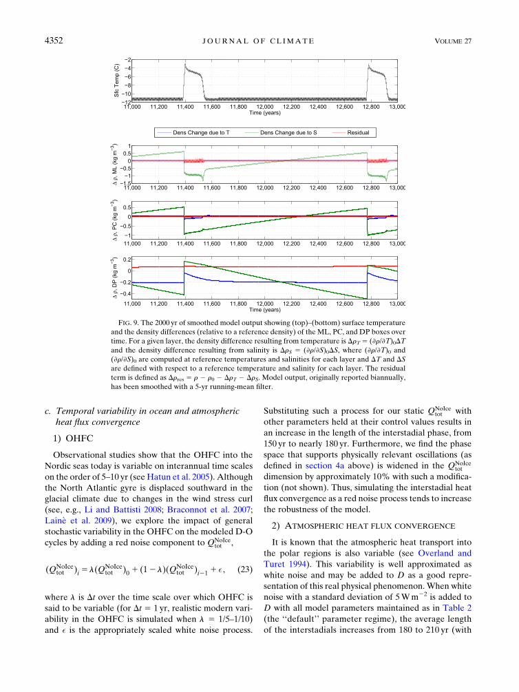
FIG. 9. The 2000 yr of smoothed model output showing (top)–(bottom) surface temperature

and the density differences (relative to a reference density) of the ML, PC, and DP boxes over

time. For a given layer, the density difference resulting from temperature is DrT 5 (›r/›T)0DTand the density difference resulting from salinity is DrS 5 (›r/›S)0DS, where (›r/›T)0 and

(›r/›S)0 are computed at reference temperatures and salinities for each layer and DT and DSare defined with respect to a reference temperature and salinity for each layer. The residual

term is defined as Drres 5 r 2 r0 2 DrT 2 DrS. Model output, originally reported biannually,

has been smoothed with a 5-yr running-mean filter.


a standard deviation of 100 yr), while the average length

of a cycle remains approximately unchanged.

d. Polynya activity

Removing the polynya parameterization in the model

[settingÐ1yr(dpice/dt) dt5 0], while leaving all other pa-

rameters at their default values prevents cycling be-

tween stadial and interstadial states. Rather than

oscillating, the model remains in an interstadial state

perpetually. Retuning other model parameters does not

prevent this. Thus, one robust result from our model is

that ice production in latent heat polynyas are a pre-

requisite for D-O cycles: removing this term precludes

the system from oscillating between stadial and in-

terstadial states.

e. General sensitivity to parameter choices

Table 4 displays the general sensitivity of the model to

key parameter values. From examining the table, we see

that the parameters broadly fall into two categories:

those that tend to change the length of the stadial phase

and those that tend to change the length of the in-

terstadial phase. In a subsequent paper, we will provide

a detailed analysis of how changes in these parameters

affect the lengths of the stadial and interstadial phases

and the time scales therein. Here, we provide a brief

overview of these parameter dependencies, and at-

tempt to obtain an intuitive sense of how the behavior

of the model is affected by these different classes of

parameters.

The parameters that change the length of the stadial

phase are those that affect the rate the column becomes

buoyantly unstable and overturns. Overturning is initi-

ated by buoyant instability between the PC and DP

boxes (see section 3). Thus, parameters that affect rPCand rDP, the densities of the pycnocline and deep layers,

will tend to affect the length of the stadial phase of the

oscillation; these include Cr, the ice export factor, and

QIcetot , the OHFC. If Cr is increased, the salinity of the PC

box increases and the salinity of the DP box decreases at

a faster pace, shortening the time it takes for rPC to

equal rDP and shortening the stadial phase. Similarly, if

QIcetot is increased, the temperature of the DP box in-

creases at a faster pace, again shortening the time re-

quired for rPC to equal rDP and thus shortening the

length of the stadial phase.

The length of the interstadial phase is determined by

the longest interstadial time scale, which depends on

a combination of parameters related to the delivery of

heat into the mixed layer. During the interstadial phase,

there is a delicate balance between the rate at which heat

is delivered into the mixed layer and the rate at which it

is fluxed from the mixed layer to the atmosphere; shift-

ing this balance toward the former lengthens the in-

terstadial, while shifting it toward the latter tends to

shorten it. In general,QNoIcetot (the OHFC during ice-free

conditions) andKNoIceML2PC (the mixing coefficient between

the ML and PC boxes during ice-free conditions) are

both related to the rate at which heat is delivered into

the ML, while BT is related to the rate at which heat is

fluxed out of the ML. Increasing QNoIcetot and KNoIce

ML2PC

tends to lengthen the interstadial time scale up to a cer-

tain point beyond which further increases in these pa-

rameters prevent the system from returning to a stadial

phase. Similarly, decreasing BT tends to lengthen the

interstadial phase up to a certain point, when any further

FIG. 10. Schematic figure depicting the key processes charac-

terizing the stadial and interstadial periods, which all result from

differences in the sea ice cover in the two states. During the in-

terstadial period, the substantial seasonal cycle of sea ice results in

large freshwater and brine fluxes into the ML and PC. Further-

more, the seasonal ice cover of the interstadial fosters more wind-

driven mixing between the ML and PC boxes, less ice export and

accompanying freshwater recirculation, and OHFC into the sur-

face layers. In contrast, the muted seasonal cycle of sea ice during

the stadial phase results in smaller melt and brine rejection fluxes.

The thicker, year-round sea ice cover of the stadial, which is aug-

mented by polynya ice import, inhibits wind-driven mixing between

the ML and PC boxes, enhances ice export and accompanying

freshwater circulation, and diverts OHFC from the surface layers

into the DP box.

15 JUNE 2014 S I NGH ET AL . 4353

decreases tend to prevent the system from returning to

the stadial.

5. Discussion and implications

a. Discussion

As with any idealized model, the purpose of our

model is to illuminate the essential ingredients re-

sponsible for the gross characteristics of D-O cycles,

particularly the time scales of the stadial and interstadial

phases, the abrupt transition from stadial to interstadial

phase, and the gentler transition back from the in-

terstadial to the stadial phase. Our results show that

a model of the area-averaged conditions in the Nordic

seas that combines an energy-balance atmosphere,

a one-layer sea ice model (which includes parameteri-

zations of polynyas, ice export, and fractional ice cover),

and four stacked ocean boxes (representing the gross

hydrographic structure of the Nordic seas) can exhibit

the gross characteristics of the D-O cycles, including

the observed hydrographic structure (Rasmussen and

Thomsen 2004; Dokken et al. 2013), the time scales as-

sociated with the stadial and interstadial phases, and the

time scales associated with the transitions between

phases.

Proxy data from the GRIP and GISP ice cores show

that the D-O oscillations occur with a periodicity of

approximately 1500 yr, with the length of the interstadial

phase persisting anywhere between 100 and 1000 yr and

the stadial phase occupying the remainder of the period

(Rahmstorf 2002). Ourmodel compares reasonably with

these observations: within the explored parameter space

where physically relevant oscillations exist, the total

length of a modeled D-O cycle is anywhere from 1000 to

1500 yr and the length of the interstadial phase is any-

where from 75 to 500 yr. While the total length of the

modeled cycle and the length of the stadial phase agree

well with observational data, the length of the modeled

interstadial phase is significantly shorter than that seen

in the proxy record.

According to the ice core record, the transitions from

the stadial to interstadial phase appear to be nearly in-

stantaneous in the Greenland record, suggesting a time

scale of less than 20yr for this transition (i.e., the temporal

resolution of the Greenland ice cores record). Our model

results show transitions from the stadial to the interstadial

FIG. 11. Model sensitivity to OHFC parametersQNoIcetot (ice free) andQIce

tot (ice covered). The

contours represent the average length of the interstadial phase (in years), while the color shades

represent the average length of the entire cycle (in years). Areas that do not support D-O-type

oscillations have been shaded in gray.


phase occur in less than 5yr, consistent with the observa-

tions. In contrast, the transition from the interstadial to the

stadial phase in the ice core records appears to take over

100 yr and possibly longer. Our model results, however,

show this transition occurs within 20–40 yr, which rep-

resents a significant disagreement with observations.

In summary, we find that there are two major dis-

crepancies between our modeled oscillations and those

seen in the proxy record: in our model the length of in-

terstadial phase is too short compared to observations

and the length of the transition from the interstadial to

stadial phase is too abrupt. These differences may be

a result of missing physics in our model, or they may be

a result of the coarse layering of the ocean column, the

lack of horizontal resolution within the Nordic seas, or

the absence of stochastic processes. We have gauged the

sensitivity of our model to stochastic variations in the

OHFC and atmospheric heat transport (see section 4a)

and found that adding this variability increased the

length of the interstadial phase, though not enough to

account for the discrepancy from observations. We be-

lieve that future work on this hypothesis could focus on

accurate modeling of horizontal transport and mixing

processes within the Nordic seas as well as on increasing

the vertical resolution of the ocean column.

We also note that our model results are consistent

with observational inferences (see section 1a) that in-

dicate a stadial increase in deep temperature of 28Cprior to overturning (Rasmussen and Thomsen 2004;

Dokken et al. 2013). Additionally, our results corrobo-

rate other observational inferences suggesting rigorous

sea ice production and accompanying brine rejection

along the FSIS is essential for D-O cycles (Dokken et al.

2013).

The model results of Winton and Sarachik (1993),

Loving and Vallis (2005), and de Verdi�ere and Raa

(2010) feature oscillations in the AMOC that are remi-

niscent of the observed D-O cycles. By contrast, our

TABLE 2. Values of constants and default parameter values used to

generate model results.

Depth of ocean boxes (m)

Depth of ML hML 50

Depth of PC hPC 300

Depth of DP hDP 800

Depth of AB hAB 3000

Mixing coefficients (m2 s21)

KT2IceML2PC 1.0 3 1024

KS2IceML2PC 1.0 3 1024

KT2NoIceML2PC 6.0 3 1024

KS2NoIceML2PC 6.0 3 1024

KTPC2DP 1.0 3 1025

KSPC2DP 1.0 3 1026

KTDP2AB 1.0 3 1027

KSDP2AB 1.0 3 1028

Optical depths

ns, ice covered 2.8

ns, ice free 2.9

nw, ice covered 2.5

nw, ice free 2.5

Other ice and ML parameters

aice 0.65

aocn 0.1

Ice–ocean conductive flux constant

C0 (Wm22 8C21)

20

Atmospheric heat transport D (Wm22) 90

OLR constant A (Wm22) 320

Temperature-dependent OLR constant

B (Wm22 8C21)

4.6

Summer shortwave radiation FSW (Wm22) 200

ML turbulent heat flux parameter

BT (Wm22 8C21)

5.0

Thermal conductivity of sea ice

k (Wm21 8C21)

2.0

Brine and polynya parameters

Range of hice in which polynyas add ice to

the column (m)

[1.0, ‘)

Ice added by polynyas each year hpolynasice (m) 1.0

Sea ice export residual brine Cr 0.05

Fraction of freshwater recirculation flux

into PC FPC

0.80

OHFC parameters (Wm22)

Ice-free OHFC QNoIcetot 3.0

Ice-covered OHFC QIcetot 0.5

TABLE 3. Sensitivity of the model to changes in the relative

distribution of the ocean heat flux distribution in the mixed layer

and pycnocline boxes during ice-free conditions. All parameters

are as in the control case but with BT 5 5.5Wm22 8C21.

Heat flux convergence distribution,

QtransML,NoIce:Q

transPC,NoIce

Interstadial length,

cycle duration

1:1 180,

1170

2:1 110,

1210

3:1 85,

1245

TABLE 4. General sensitivity of the model time scales (length of

stadial phase and length of interstadial phase) to changes in model

parameters.

Parameter change Effect on stadial Effect on interstadial

Increase BT Little effect Shorten

Increase Cr Shorten Little effect

Increase QIcetot Shorten Little effect

Increase QNoIcetot Little effect Lengthen

Increase dpice/dt More ice Shorten

Increase ice threshold

for polynyas

Little effect Lengthen

Increase KNoIceML2PC Little effect Lengthen

15 JUNE 2014 S I NGH ET AL . 4355

model features D-O cycles resulting from interactions

within an atmosphere–sea ice–ocean column, rather

than within an Atlantic Ocean scale model: changes in

the ocean stratification and sea ice cover within the

Nordic seas that are the hallmark of our model D-O

cycles are independent of any changes in the heat and

salt transport associated with the AMOC. In fact, our

model suggests that D-O cycles will only exist if the

sinking branch of the AMOC does not extend into the

Nordic seas (as it does in the present climate): the system

will only support a stadial state when ocean heat trans-

port into the Nordic seas is less than 0.005 PW (3Wm22

averaged over the area of the Nordic seas), which is

a small fraction of what is delivered into the Nordic seas

today.

In general, we hypothesize that ocean heat transport

incident on an ice-covered regionwill tend to subduct and

circulate under a cold halocline, while ocean heat trans-

port incident on a region that is ice free will tend to

concentrate in the upper ocean and converge there while

it fluxes into the atmosphere. In the former case, very

little heat will converge into the region, while in the latter

case, a slightly larger amount of heat will converge.

Hence, the sea ice cover causes changes in the distribu-

tion of OHFC that feed back on the sea ice cover itself.

Work by Bitz et al. (2006) usedGCMresults to argue that

transitioning from perennial to seasonal sea ice in the

Arctic enhanced brine rejection along the Siberian shelf,

resulting in an increase in theOHFC into the region. Such

changes occurred despite a weakening in the strength of

the AMOC south of the subpolar seas (Bitz et al. 2006).

Thus, the OHFC changes we prescribe account for dif-

ferences in the vertical distribution of how heat converges

locally in the presence or absence of sea ice and a cold

halocline and are independent of the AMOC.

Consistent with the small value of OHFC, the only

advective salt flux convergence (ASFC) in our model is

into the DP box, and it is used to balance the freshwater

flux out of the Nordic seas associated with sea ice export.

Physically, we envision that exported sea ice melts in

the North Atlantic, entrains into the sinking branch of

the AMOC, and returns at depth to the Nordic seas. The

lack of ASFC into the top two boxes is supported by

GCM simulations run with Last Glacial Maximum

(LGM) boundary conditions, which show that theASFC

into the Nordic seas is very small [see Braconnot et al.

2007; see also the Paleoclimate Modelling Intercom-

parison Project 2 (PMIP2) archive].

In our model, the slight difference in the magnitudes

of the ice-covered and ice-free OHFC only affects the

details of the modeled oscillations, not the oscillations

themselves or the hydrographic structures of the stadial

and interstadial phases. Imposing an ice-covered and

ice-free OHFC that are both equal to 1Wm22, for ex-

ample, results in modeled D-O oscillations with an in-

terstadial phase of 150 yr and a full cycle period of

850 yr.

Modeling results (Brandefelt and Otto-Bliesner 2009)

support our assumption that the Nordic seas were rela-

tively disconnected from theAMOC throughout the last

glacial period. In the modern climate, the wind-driven

subpolar gyre efficiently delivers heat and salt into the

Nordic seas; as a result, the sinking branch of theAMOC

resides in the Nordic seas. In the glacial climate, how-

ever, GCM simulations suggest that the Laurentide ice

sheet deflected the atmospheric jet southward and re-

duced the storminess over the NorthAtlantic (Braconnot

et al. 2007; Laın�e et al. 2009). Consistent with the south-

ward deflection of the jet, long-equilibration coupled

climatemodel simulations (Brandefelt andOtto-Bliesner

2009) suggest the AMOC was weaker and shallower

during the glacial period and the sinking branch was

shifted southward from today’s position in the Nordic

seas.

b. Implications

Our model helps explain why D-O cycles are not

present in theHolocene. As discussed in section 4e, D-O

cycles are only possible when the ocean heat imported to

the Nordic seas is small, less than 0.005 PW (3Wm22

multiplied by the area of the Nordic seas). The OHFC

into theNordic seas today is about 0.05 PW (Hansen and

Osterhus 2000), which is an order of magnitude higher.

Further reasons why the Nordic seas do not experi-

ence stadial conditions and D-O-type oscillations during

the Holocene may also include the current position of

the midlatitude storm track and the lack of substantial

polynya activity, both of which make it difficult to form

a strong halocline in the region today. Today, the mid-

latitude storm track traverses the Nordic seas; during

glacial times, on the other hand, proxy evidence (see

Pailler and Bard 2002) and modeling results (see, e.g.,

Li and Battisti 2008; Braconnot et al. 2007; Laın�e et al.

2009) suggest that the midlatitude storm track was

shifted equatorward from its current position. While

conditions within the Nordic seas during the last glacial

period may have been quiescent enough to support the

formation of a strong halocline, the current position of

the storm track may preclude the existence of a halo-

cline because of significant wind-driven mixing of the

upper ocean in the region. Without a halocline, sea ice

formed in the region (if any) would be unable to persist

because of heat fluxes from warmer waters below. In the

Arctic basin today, the presence of a strong halocline

is crucial for preventing warmer circulating Atlantic

waters below from melting the sea ice (Aagaard et al.


1981). In addition to the current position of the storm

track, the lack of polynya activity in theHolocene would

also make it more difficult to form a strong halocline.

The proxy record of the last glacial period presents

another interesting conundrum regarding millennial-

scale variability: D-O oscillations, which were robust

and plentiful during the glacial period prior to 24 kyr

before present, were absent during the LGM itself. The

results of our model suggest that latent heat polynyas,

which formed off the edge of the Fennoscandian ice

sheet (FSIS) during the last glacial period, were essential

for the D-O oscillations: polynyas are required for re-

turning the Nordic seas to the stadial phase of the D-O

cycle and for maintaining the stratification between the

ML and PC throughout the stadial phase. During the

LGM, the FSIS was believed to extend to the conti-

nental shelf. While katabatic winds would have still

emanated from the FSIS in this case and latent heat

polynyas would still result, conditions would have been

much colder with more brine rejected. The continental

slope bathymetry over which the brine rejected from

such polynyas would traverse would be much different

from the extensive continental shelf over which it flowed

and entrained during the glacial. In the former case, it is

possible that the resulting large volume of cold brine

flowing down the continental slope could not entrain

enough ambient water to interleave into the halocline.

Consequently, the brine would sink to the bottom of the

water column, in a manner analogous to deep-water

formation in coastal polynyas in the present-dayWeddell

Sea. Thus, it is possible that the region only supported

a weak halocline, and incoming heat from the North

Atlantic converged into the deep would not be trapped

and decoupled from the surface (as we hypothesize is

characteristic of the stadial phases of the D-O cycles) but

rather gradually vented, reducing the thickness of the sea

ice in the Nordic seas. In such a case, there would be in-

sufficient buildup of deep ocean heat and pycnocline salt

to initiate a convective overturning event, and the Nordic

seas would remain in a perpetual stadial phase.

Acknowledgments. We wish to acknowledge grants

from the Comer Foundation and the U.S. Department

of Energy Computational Science Graduate Fellowship

(DOECSGF); Aaron Barker for composing Fig. 10; and

the helpful comments, suggestions, and critiques of three

anonymous reviewers, whose thoughtful input improved

the quality of the work substantially.

REFERENCES

Aagaard, K., L. K. Coachman, and E. Carmack, 1981: On the

halocline of the Arctic Ocean. Deep-Sea Res., 28A, 529–545,

doi:10.1016/0198-0149(81)90115-1.

Alley, R., 2007: Wally was right: Predictive ability of the North

Atlantic conveyer belt hypothesis for abrupt climate change.

Annu. Rev. Earth Planet. Sci., 35, 241–272, doi:10.1146/

annurev.earth.35.081006.131524.

Bitz, C. M., P. R. Gent, R. A. Woodgate, M. M. Holland, and

R. Lindsay, 2006: The influence of sea ice on ocean heat up-

take in response to increasing CO2. J. Climate, 19, 2437–2450,

doi:10.1175/JCLI3756.1.

——, J. C. H. Chiang, W. Cheng, and J. J. Barsugli, 2007: Rates

of thermohaline recovery from freshwater pulses in modern,

Last Glacial Maximum and greenhouse warming climates.

Geophys. Res. Lett., 34, L07708, doi:10.1029/2006GL029237.

Bond, G. C., and R. Lotti, 1995: Iceberg discharges into

the North Atlantic on millennial time scales during the

last glaciation. Science, 267, 1005–1010, doi:10.1126/

science.267.5200.1005.

Braconnot, P., and Coauthors, 2007: Results of PMIP2 coupled

simulations of Mid-Holocene and Last Glacial Maximum—

Part 1: Experiments and large-scale features. Climate Past, 3,

261–277, doi:10.5194/cp-3-261-2007.

Brandefelt, J., and B. Otto-Bliesner, 2009: Equilibration and

variability in a Last Glacial Maximum climate simulation

with CCSM3. Geophys. Res. Lett., 36, L19712, doi:10.1029/

2009GL040364.

Cavalieri, D., and S. Martin, 1994: The contribution of Alaskan,

Siberian, and Canadian coastal polynyas to the cold halocline

layer of the Arctic Ocean. J. Geophys. Res., 99 (C9), 18 343–

18 362, doi:10.1029/94JC01169.

Chiang, J. C. H., and C. M. Bitz, 2005: Influence of high latitude ice

cover on the marine intertropical convergence zone. Climate

Dyn., 25, 477–496, doi:10.1007/s00382-005-0040-5.

——,M. Biasutti, andD. S. Battisti, 2003: Sensitivity of theAtlantic

intertropical convergence zone to Last Glacial Maximum

boundary conditions. Paleoceanography, 18, 1094, doi:10.1029/

2003PA000916.

Clement, A., and L. Peterson, 2008: Mechanisms of abrupt climate

change of the last glacial period. Rev. Geophys., 46, RG4002,

doi:10.1029/2006RG000204.

Dansgaard, W., S. Johnsen, H. Clausen, D. Dahl-Jensen,

N. Gundestrup, C. Hammer, and H. Oeschger, 1984: North

Atlantic climatic oscillations revealed by deep Greenland ice

cores. Climate Processes and Climate Sensitivity, Geophys.

Monogr., Vol. 29, Amer. Geophys. Union, 288–298.

——, and Coauthors, 1993: Evidence of general instability of past

climate from a 250-kyr ice core record. Nature, 364, 218–220,

doi:10.1038/364218a0.

de Verdi�ere, A., and L. Raa, 2010: Weak oceanic heat transport as

a cause of the instability of glacial climates. Climate Dyn., 35,

1237–1256, doi:10.1007/s00382-009-0675-8.

Dokken, T. M., and E. Jansen, 1999: Rapid changes in the mode of

deep and intermediate water formation linked with atmo-

spheric and ice sheet variations during the last glacial.Nature,

401, 458–461, doi:10.1038/46753.

——, K. H. Nisancioglu, C. Li, D. S. Battisti, and C. Kissel, 2013:

Dansgaard-Oeschger cycles: Interactions between ocean and

sea ice intrinsic to theNordic seas.Paleoceanography, 28, 491–

502, doi:10.1002/palo.20042.

Duffy, P. B., M. Eby, and A. J. Weaver, 1999: Effects of sinking of

salt rejected during formation of sea ice on results of an ocean-

atmosphere-sea ice climate model. Geophys. Res. Lett., 26,

1739–1742, doi:10.1029/1999GL900286.

Elliot, M., L. Labeyrie, T. Dokken, and S. Manth�e, 2001: Coherent

patterns of ice rafted debris deposits in the Nordic regions

15 JUNE 2014 S I NGH ET AL . 4357

during the last glacial (10–60 ka). Earth Planet. Sci. Lett., 194,

151–163, doi:10.1016/S0012-821X(01)00561-1.

——, ——, and J.-C. Duplessy, 2002: Changes in North Atlantic

deep-water formation associated with the Dansgaard–Oeschger

temperature oscillations (60–10ka). Quat. Sci. Rev., 21, 1153–

1165, doi:10.1016/S0277-3791(01)00137-8.

Ganopolski, A., and S. Rahmstorf, 2001: Rapid changes of glacial

climate simulated in a coupled climate model. Nature, 409,153–158, doi:10.1038/35051500.

Gargett, A., 1984: Vertical eddy diffusivity in the ocean interior.

J. Mar. Res., 42, 359–393, doi:10.1357/002224084788502756.

Gill, A. E., 1982: Atmosphere-Ocean Dynamics. Academic Press,

662 pp.

Hansen, B., and S. Osterhus, 2000: North Atlantic-Nordic

seas exchanges. Prog. Oceanogr., 45, 109–208, doi:10.1016/S0079-6611(99)00052-X.

Hatun, H., A. Sando, H. Drange, B. Hansen, and H. Valdimarsson,

2005: Influence of the Atlantic subpolar gyre on the ther-

mohaline circulation. Science, 309, 1841–1844, doi:10.1126/science.1114777.

Huppert, H., and J. Turner, 1981: Double-diffusive convection.

J. Fluid Mech., 106, 299–329, doi:10.1017/S0022112081001614.

Keigwin, L., and E. Boyle, 1999: Surface and deep ocean variability

in the northern Sargasso Sea during marine isotope stage 3.

Paleoceanography, 14, 164–170, doi:10.1029/1998PA900026.

Kraus, E., and J. Turner, 1967: A one-dimensional model of the sea-

sonal thermocline II. The general theory and its consequences.

Tellus, 19, 98–106, doi:10.1111/j.2153-3490.1967.tb01462.x.

Laın�e, A., and Coauthors, 2009: Northern Hemisphere storm

tracks during the last glacial maximum in the PMIP2 ocean-

atmosphere coupled models: Energetic study, seasonal cy-

cle, precipitation. Climate Dyn., 32, 593–614, doi:10.1007/

s00382-008-0391-9.

Li, C., and D. Battisti, 2008: Reduced Atlantic storminess during

the Last Glacial Maximum: Evidence from a coupled climate

model. J. Climate, 21, 3561–3579, doi:10.1175/2007JCLI2166.1.

——, ——, D. Schrag, and E. Tziperman, 2005: Abrupt climate

shifts in Greenland due to displacements in the sea ice edge.

Geophys. Res. Lett., 32, L19702, doi:10.1029/2005GL023492.

Loving, J. L., and G. K. Vallis, 2005: Mechanism for climate vari-

ability during glacial and interglacial periods. Paleoceanog-

raphy, 20, PA4024, doi:10.1029/2004PA001113.

MacAyeal, D., 1993: Binge/purge oscillations of the Laurentide ice

sheet as a cause of the North Atlantic’s Heinrich events. Pa-

leoceanography, 8, 775–784, doi:10.1029/93PA02200.

Martin, S., R. Drucker, and K. Yamashita, 1998: The production of

ice and dense shelf water in the Okhotsk Sea polynyas. J. Geo-

phys. Res., 103 (C12), 27771–27782, doi:10.1029/98JC02242.

Nguyen, A., D. Menemenlis, and R. Kwok, 2009: Improved mod-

eling of the Arctic halocline with a subgrid-scale brine re-

jection parameterization. J. Geophys. Res., 114, C11014,

doi:10.1029/2008JC005121.

Okumura, Y., C. Deser, A. Hu, A. Timmermann, and S. Xie, 2009:

North Pacific climate response to freshwater forcing in the

subarctic North Atlantic: Oceanic and atmospheric pathways.

J. Climate, 22, 1424–1445, doi:10.1175/2008JCLI2511.1.Otto-Bliesner, B., andE. Brady, 2010: The sensitivity of the climate

response to the magnitude and location of freshwater forcing:

Last Glacial Maximum experiments. Quat. Sci. Rev., 29, 56–

73, doi:10.1016/j.quascirev.2009.07.004.

Overland, J., and P. Turet, 1994: Variability of the atmospheric

energy flux across 708N computed from the GFDL data set.

The Polar Oceans and Their Role in Shaping the Global En-

vironment, Geophys. Monogr., Vol. 85, Amer. Geophys. Un-

ion, 313–325.

Pailler, D., and E. Bard, 2002: High frequency palaeoceano-

graphic changes during the past 140,000 year recorded by the

organic matter in sediments of the Iberian Margin. Palae-

ogeogr. Palaeoclimatol. Palaeoecol., 181, 431–452, doi:10.1016/

S0031-0182(01)00444-8.

Pausata, F., D. Battisti, K. Nisancioglu, and C. Bitz, 2011: Chinese

stalagmites: Proxies for the Indian monsoon response to an

archetypal Heinrich event.Nat. Geosci., 4, 474–480, doi:10.1038/

ngeo1169.

Peixoto, J. P., and A. H. Oort, 1992: Physics of Climate. American

Institute of Physics, 520 pp.

Rahmstorf, S., 2002: Ocean circulation and climate during the past

120,000 years. Nature, 419, 207–214, doi:10.1038/nature01090.

Rasmussen, T., and E. Thomsen, 2004: The role of the North At-

lantic drift in the millennial timescale glacial climate fluctua-

tions. Palaeogeogr. Palaeoclimatol. Palaeoecol., 210, 101–116,

doi:10.1016/j.palaeo.2004.04.005.

Schmittner, A., and T. Stocker, 2001: A seasonally forced ocean–

atmosphere model for paleoclimate studies. J. Climate, 14, 1055–

1068, doi:10.1175/1520-0442(2001)014,1055:ASFOAM.2.0.CO;2.

Semtner, A., 1976: A model for the thermodynamic growth of

sea ice in numerical investigations of climate. J. Phys.

Oceanogr., 6, 379–389, doi:10.1175/1520-0485(1976)006,0379:

AMFTTG.2.0.CO;2.

Stouffer, R. J., and Coauthors, 2006: Investigating the causes of

the response of the thermohaline circulation to past and fu-

ture climate changes. J. Climate, 19, 1365–1387, doi:10.1175/

JCLI3689.1.

Swingedouw,D., J.Mignot, P. Braconnot, E.Mosquet,M.Kageyama,

and R. Alkama, 2009: Impact of freshwater release in the North

Atlantic under different climate conditions in an OAGCM.

J. Climate, 22, 6377–6403, doi:10.1175/2009JCLI3028.1.Thorndike, A., 1992: A toy model linking atmospheric thermal

radiation to sea ice growth. J. Geophys. Res., 97 (C6), 9401–

9410, doi:10.1029/92JC00695.

Vellinga, M., and R. Wood, 2002: Global climatic impacts of

a collapse of the Atlantic thermohaline circulation. Climatic

Change, 54, 251–267, doi:10.1023/A:1016168827653.

Weaver, A., E. Sarachik, and J. Marotze, 1991: Freshwater flux

forcing of decadal and interdecadal ocean variability. Nature,

353, 836–838, doi:10.1038/353836a0.

Welander, P., 1977: Thermal oscillations in a fluid heated from

below and cooled to freezing from above. Dyn. Atmos.

Oceans, 1, 215–223, doi:10.1016/0377-0265(77)90007-0.——, 1982: A simple heat-salt oscillator. Dyn. Atmos. Oceans, 6,

233–242, doi:10.1016/0377-0265(82)90030-6.

——, and J. Bauer, 1977: On a differentially heated saltwater-ice sys-

tem. Tellus, 29, 462–469, doi:10.1111/j.2153-3490.1977.tb00757.x.

Winton, M., and E. Sarachik, 1993: Thermohaline oscillations

induced by strong steady salinity forcing of ocean general

circulation models. J. Phys. Oceanogr., 23, 1389–1410,

doi:10.1175/1520-0485(1993)023,1389:TOIBSS.2.0.CO;2.

Wunsch, C., and R. Ferrari, 2004: Vertical mixing, energy, and the

general circulation of the oceans. Annu. Rev. Fluid Mech., 36,

281–314, doi:10.1146/annurev.fluid.36.050802.122121.


Documents

A Heuristic Model of Dansgaard–Oeschger Cycles. Part I