Embed Size (px)
Citation preview

A GUIDEBOOK ON THE USE OF SATELLITE
GREENHOUSE GASES OBSERVATION DATA
TO EVALUATE AND IMPROVE GREENHOUSE GAS
EMISSION INVENTORIES
1st EDITION
MARCH 2018
NATIONAL INSTITUTE FOR ENVIRONMENTAL STUDIES,
JAPAN

Revision History
March 31, 2018: Revision 12a
April 5, 2018: Revision 12b
Map in the cover page : GOSAT observed XCO2 anomalies averaged over 2° × 2° grid over anthropogenic sources regions over the globe for 2009–2012. See Section 4.4 for more details.
This document may be cited as:
Matsunaga T. and Maksyutov S (eds) (2018) A Guidebook on the Use of Satellite Greenhouse
Gases Observation Data to Evaluate and Improve Greenhouse Gas Emission Inventories, Satellite
Observation Center, National Institute for Environmental Studies, Japan, 129 pp.
Contact : Dr. Tsuneo Matsunaga ([email protected]), Satellite Observation Center, National
Institute for Environmental Studies, 16-2 Onogawa Tsukuba Ibaraki 305-8506 Japan.

Preface
Preface
The Paris Agreement, which entered into force on November 4, 2016, is the world’s first
framework to deal with climate change through both “mitigation” measures to reduce greenhouse
gas (GHG) emissions and “adaptation” to the impacts of climate change. All nations started to take
action to comply with the Paris Agreement, which has been ratified by 159 countries including
developed and developing countries and the European Union as of September 2017.
The Paris Agreement defines a mechanism of “global stocktake” that all nations set the GHG
reduction targets, report each progress, and assess the collective progress towards achieving the
goals every five years after 2020.
Each country is required to report its national GHG emissions inventory under a highly
transparent framework. To secure the transparency of the inventory, a system is necessary to
compare and evaluate the inventories by some independent ways. One of the ways is a GHG
observation method using satellite remote sensing techniques that Japan and other countries are
working on.
In Japan, under a joint project by the Ministry of the Environment (MOE), the National
Institute for Environmental Studies (NIES), and the Japan Aerospace Exploration Agency (JAXA),
the Greenhouse gases Observing SATellite (GOSAT) “IBUKI” was launched as the world’s first
satellite dedicated to monitoring greenhouse gases in January 2009. The satellite has been observing
global GHGs such as carbon dioxide (CO2) and methane (CH4) and monitoring their fluctuations
for nine years since its launch.
With the “IBUKI” observations and the full use of ground-based and aircraft observations and
modeling techniques, we have recently found the following trends for the first time in the world:
whole-atmosphere monthly mean CO2 concentrations reaching 406 ppm and CH4 recording 1824
ppb in January 2018 with an annual increase with seasonal variations. In addition, we released the
estimates of anthropogenic CO2 and CH4 emissions, which marked the first step towards utilizing
the “IBUKI” series for environmental policy.
These observation outcomes leveraging the advantages of the satellite are contributing to the
precise predictions of climate change. In addition, they become basic information for monitoring
domestic and international efforts to reduce GHG emissions. We have been developing a successor
“IBUKI-2” (GOSAT-2) to be launched in FY2018 and striving to advance techniques to assess and
validate GHG emissions in large cities and large-scale emission sources using the IBUKI-2
observations.
On the other hand, in the United States, NASA launched the Orbiting Carbon Observatory 2
(OCO-2) in July 2014 and has been in operation. This satellite aims to characterize CO2 sources and
sinks on regional scales and quantify CO2 variability over the seasonal cycles. The project teams of

Preface
OCO-2, GOSAT, and GOSAT-2 have been enforcing cooperative relationships from an early stage
and making an effort to improve the accuracy of the data products by cross-calibration and
validation under the Memorandum of Understanding among MOE, JAXA, NIES, and NASA,
which was signed in March 2015.
In December 2017, JAXA and NIES made collaboration agreements with the European Space
Agency (ESA), with the Centre National D’Etudes Spatiales (CNES), and with the German
Aerospace Center (DLR). These agreements aim to increase the reliability of satellite GHG data and
achieve its uniformity by cross-calibration and validation among the data from GOSAT, GOSAT-2,
and GHG observing satellites operated or to be launched by European agencies.
To utilize these space-based GHG measurements for the system of estimating and evaluating
each nation’s GHG emissions, there are many possible challenges because innovative techniques
are necessary. For example, one of the issues is technical assistance for inventory compilers in areas
not having inventory data with high quality to compile and evaluate the GHG emissions inventories.
It is necessary that Japan will cooperate internationally not only in a technical aspect such as
analyzing satellite remote sensing data, but also in capacity building activities including training
courses for inventory compilers through association with international organizations and
development agencies.
We hope that this guidebook will be a good opportunity to introduce remote sensing techniques
by GHG observation satellites as one of the methods for estimating and evaluating each nation’s
GHG emissions. As a result, we also hope that this guidebook will lead to taking further measures
against global warming.
Masanobu Kimura
Director
Research and Information Office
Global Environment Bureau
Ministry of the Environment Japan

Contents
i
CONTENTS Preface
Contents
Acknowledgements
About This Guidebook
Chapter 1 OVERVIEW -1-1-
1.1 Background -1-1-
1.2 Objective of this guidebook -1-3-
1.3 Structure of this guidebook -1-3-
Chapter 2 SATELLITE OBSERVATIONS AND DATA APPLICATIONS, PART 1:
SATELLITE OBSERVATIONS, GHG CONCENTRATION RETRIEVALS AND
VALIDATION -2-1-
2.1 Introduction -2-1-
2.2 Brief history of satellite remote sensing of greenhouse gases -2-4-
2.3 Products of satellite remote sensing of greenhouse gases -2-8-
2.4 Retrieval algorithms to derive greenhouse gas concentrations from SWIR spectral
data -2-9-
2.5 Validation of column concentrations derived from satellite SWIR data -2-11-
Chapter 3 SATELLITE OBSERVATIONS AND DATA APPLICATIONS, PART. 2: USING
SATELLITE OBSERVATIONS FOR EMISSION ESTIMATES AND
COMPARISON TO EMISSION INVENTORIES -3-1-
3.1 Emission estimates based on analysis of concentration anomalies around emission
sources -3-1-
3.2 Anthropogenic GHG emission estimates based on inverse modeling -3-5-
Chapter 4 CASE STUDIES -4.0-1-
4.1 Anthropogenic CO2 emission trends from SCIAMACHY/ENVISAT and
comparison with EDGAR -4.1-1-
4.2 Direct space-based Observations of Anthropogenic CO2 Emission Areas: Global
Contents
ii
XCO2 Anomalies -4.2-1-
4.3 Using space-based observations to study urban CO2 emissions and CH4 emissions
from fossil fuel harvesting -4.3-1-
4.4 Monitoring anthropogenic CO2 and CH4 emission by GOSAT observations -4.4-1-
4.5 Anthropogenic methane emissions from SCIAMACHY and GOSAT -4.5-1-
4.6 A case study estimating global and regional methane emissions using GOSAT-4.6-1-
4.7 Joint analysis of CO2 and CH4 inversion fluxes to refine anthropogenic CO2
emissions: A case study of East Asia -4.7-1-
4.8 Inversion modeling of global CH4 emissions: results for sub-continental regions of
Asia and outlook for satellite data utilization -4.8-1-
4.9 Quantifying CO2 Emissions from Individual Power Plants from Space -4.9-1-
Appendix-1 REFERENCES -Appendix 1-1-
Appendix-2 ACRONYMS AND ABBREVIATIONS -Appendix 2-1-
Appendix-3 LIST OF GREENHOUSE GAS MEASURING SATELLITES -Appendix 3-1-

Acknowledgements
ACKNOWLEDGEMENTS
The preparation and review of this guidebook has been supported by many individuals. We
would like to thank the authors and co-authors of Chapter 4 for descriptions of their studies. In
addition, the participants in the first and second expert meetings on the guidebook held in Tokyo in
2017 and 2018 are acknowledged for providing presentations and useful advice to prepare and
improve the guidebook. Finally, appreciation is extended to many scientists and other contributors
for providing helpful comments and suggestions on the draft edition of the guidebook. Especially,
support for the revision of Section 1.1 and 2.1, provided by David Crisp, Eric Kort, Ray Nassar, and
Alexander Turner, is sincerely appreciated. All the contributors are listed in the table below. We are
most grateful for their valuable contributions.
The production of this guidebook has been financially supported by the Ministry of the
Environment, Japan (MOE).
Tsuneo Matsunaga, Shamil Maksyutov, and Tomoko Kanno
National Institute for Environmental Studies (NIES), Japan
Name Affiliation Contribution
1 Aoki, Shuji Tohoku University, Japan Chapter 4 Co-author
2 Bito, Chika NIES Participant in the 1st expert meeting
3 Boer, Rizaldi Bogor Agricultural
University, Indonesia
Participant in the 1st and 2nd expert
meetings
4 Bovensmann, H. University of Bremen,
Germany
Chapter 4 Co-author
5 Briggs, Stephen European Space Agency,
Italy
Providing comments on the draft
edition
6 Buchwitz, Michael University of Bremen,
Germany
Chapter 4 Lead author and Participant
in the 1st and 2nd expert meetings via
Skype
7 Burrows, J. P. University of Bremen,
Germany
Chapter 4 Co-author
8 Butz, Andre German Aerospace Center
(DLR), Germany
Chapter 4 Co-author
9 Chijimatsu, Satoshi MOE Participant in the 1st expert meeting
10 Counet, Paul EUMETSAT, Germany Providing comments on the draft
edition

Acknowledgements
11 Crisp, David California Institute of
Technology, USA
Chapter 4 Co-author and Participant in
the 2nd expert meeting
12 Dlugokencky,
Edward J.
National Oceanic and
Atmospheric
Administration, USA
Chapter 4 Co-author
13 Endo, Takahiro Remote Sensing
Technology Center of
Japan (RESTEC), Japan
Participant in the 1st and 2nd expert
meetings
14 Ganesan, Anita University of Bristol, UK Participant in the 2nd expert meeting
via Skype
15 Hakkarainen, Janne Finnish Meteorological
Institute (FMI), Finland
Chapter 4 Lead author and Participant
in the 1st and 2nd expert meetings
16 Hatanaka, Elsa NIES Participant in the 1st and 2nd expert
meetings
17 Hill, Timothy G. University of Waterloo,
Canada
Chapter 4 Co-author
18 Ialongo, Iolanda FMI Chapter 4 Co-author
19 Imasu, Ryoichi University of Tokyo,
Canada
Participant in the 1st and 2nd expert
meetings
20 Inanaga, Asako RESTEC Participant in the 1st expert meeting
21 Isono, Kazuo MOE Participant in the 1st expert meeting
22 Ito, Akihiko NIES Chapter 4 Co-author
23 Ito, Hiroshi NIES Participant in the 2nd expert meeting
24 Janardanan, Rajesh NIES Chapter 4 Lead author and Participant
in the 1st and 2nd expert meetings
25 Janssens-Maenhout,
Greet
Joint Research Center,
Italy
Participant in the 1st expert meeting via
Skype
26 Jones, Dylan B.A. University of Toronto,
Canada
Chapter 4 Co-author
27 Kaewcharoen, Sivach Office of Natural
Resources and
Environmental Policy and
Planning, Thailand
Participant in the 1st and 2nd expert
meetings
28 Kimura, Masanobu MOE Participant in the 2nd expert meeting
29 Kobayashi, Kazufumi MOE Participant in the 2nd expert meeting

Acknowledgements
30 Kort, Eric University of Michigan,
USA
Chapter 4 Lead author and Participant
in the 1st and 2nd expert meetings via
Skype
31 Kosaka, Naohumi NIES Participant in the 1st expert meeting
32 Kuze, Akihide Japan Aerospace
Exploration Agency
(JAXA), Japan
Participant in the 1st expert meeting
33 Lauvaux, Thomas Pennsylvania State
University, USA
Participant in the 1st expert meeting via
Skype
34 McLinden, Chris A. Environment and Climate
Change Canada, Canada
Chapter 4 Co-author
35 Miyauchi, Seiji Japan Meteorological
Agency, Japan
Participant in the 2nd expert meeting
36 Morimoto, Shinji Tohoku University, Japan Chapter 4 Co-author
37 Nakajima, Masakatsu JAXA Participant in the 1st expert meeting
38 Nakamura, Yuko JAXA Participant in the 1st expert meeting
39 Nakazawa, Takakiyo Tohoku University, Japan Chapter 4 Co-author
40 Nassar, Ray Environment and Climate
Change Canada, Canada
Chapter 4 Lead author and Participant
in the 2nd expert meeting via Skype
41 Ninomiya, Keiichiro NIES Participant in the 1st and 2nd expert
meetings
42 Niwa, Yosuke Meteorological Research
Institute, Japan
Participant in the 1st and 2nd expert
meetings
43 Oda, Tomohiro USRA/NASA Goddard
Space Flight Center, USA
Chapter 4 Co-author and Participant in
the 1st and 2nd expert meetings
44 Prabir, Patra Japan Agency for
Marine-Earth Science and
Technology (JAMSTEC),
Japan
Chapter 4 Lead author and Participant
in the 1st and 2nd expert meetings
45 Prinn, Ronald G. Massachusetts Institute of
Technology, USA
Chapter 4 Co-author
46 Reuter, M. University of Bremen,
Germany
Chapter 4 Co-author
47 Saeki, Tazu NIES Chapter 4 Lead author and Participant
in the 2nd expert meeting

Acknowledgements
48 Saigusa, Nobuko NIES Participant in the 2nd expert meeting
49 Saito, Makoto NIES Chapter 4 Co-author and Participant in
the 1st an 2nd expert meetings
50 Schneising-Weigel, O. University of Bremen,
Germany
Chapter 4 Co-author
51 Shiomi, Kei JAXA Participant in the 1st expert meeting
52 Takemoto, Akio MOE Participant in the 1st expert meeting
53 Tamminen, Johanna FMI Chapter 4 Co-author and Participant in
the 1st expert meeting via Skype
54 Tanabe, Kiyoto Institute for Global
Environmental Strategies,
Japan
Participant in the 1st and 2nd expert
meetings
55 Tanaka, Tetsuhiro MOE Participant in the 2nd expert meeting
56 Turner, Alexander University of California at
Berkeley, USA
Chapter 4 Lead author and Participant
in the 1st and 2nd expert meetings via
Skype
57 Uchida, Miyuki NIES Participant in the 1st expert meeting
58 Ueno, Mikio Japan Meteorological
Agency, Japan
Participant in the 1st and 2nd expert
meetings
59 Urita, Shinji MOE Participant in the 1st expert meeting
60 Wunch, Debra University of Toronto,
Canada
Chapter 4 Co-author
61 Yoshida, Yukio NIES Chapter 4 Co-author

About this guidebook
This guidebook, “A Guidebook on the Use of Satellite Greenhouse Gases Observation Data to
Evaluate and Improve Greenhouse Gas Emission Inventories” (hereinafter referred to as “this
guidebook”), has been produced by the National Institute for Environmental Studies, as part of
outsourced contracts with the Ministry of the Environment, Japan in FY 2016 and 2017.
The Paris Agreement, which entered into force in 2016, is the world’s first framework to deal
with climate change through both “mitigation” measures to reduce greenhouse gas (GHG)
emissions and “adaptation” to the impacts of climate change. The Paris Agreement defines a
mechanism of “global stocktake” that all nations set the GHG reduction targets, report each
progress, and assess the collective progress towards achieving the goals every five years after 2020.
There are several ways to compile a national GHG emission inventory (hereinafter referred to
as “inventory”). The Paris Agreement requires each country to report its inventory under a highly
transparent framework. To secure the transparency of the inventory, a system is necessary to
compare and evaluate the inventories by some independent ways. One of the ways is a GHG
observation method using satellite remote sensing techniques that Japan and other countries are
working on. Especially in the field of satellite remote sensing of GHGs, research and development
has been actively promoted. Several satellites to monitor GHGs have been in operation. The
examples of such satellites include the Greenhouse gases Observing SATellite (GOSAT) launched
by Japan in 2009, the Orbiting Carbon Observatory 2 (OCO-2) by the US in 2014, and Sentinel-5p
by the European Space Agency in 2016. In addition, future plans for satellites are currently underway.
This guidebook targets each nation’s inventory compilers and researchers in the related fields.
The objective of this guidebook is to explain methodology to compare and evaluate inventories,
which all nations report under the Paris Agreement, by using satellite remote sensing techniques
(Chapter 2 and 3), and to introduce their practical case studies (Chapter 4). The case studies include
the latest research at various spatial scales from global and sub-continental level to individual
large-sized coal power plants.
All satellite GHG data introduced in this guidebook can be downloaded for free from each
satellite website.
Furthermore, capacity building activities for the inventory compilers are being considered. We
have been examining the feasibility of the activities such as conducting lectures and training
courses using this guidebook as one learning tool, and providing various data, software, and work
environment.
We hope that this guidebook and the future capacity building activities will help the inventory
compilers to widely use the methodology to compare and evaluate the inventories using satellite
remote sensing techniques towards the first global stocktake.

Chapter 1 Overview
1-1
1. OVERVIEW
1.1 Background The Earth's environment is changing rapidly and these changes are affecting natural terrestrial
and marine ecosystems, agriculture, human health, economic activity, and even national security.
Recognizing the impact of these changes, the Sustainable Development Goals (SDGs) defined by
the United Nations (UN) in 2015 include "Goal 13: Take urgent action to combat climate change
and its impacts". The rising concentrations of atmospheric greenhouse gases (GHGs) such as
carbon dioxide (CO2) and methane (CH4) are key drivers of climate change (IPCC, 2013). Since the
dawn of the industrial age, fossil fuel combustion and other human activities have increased the
atmospheric CO2 concentration by more than 40%, from less than 280 parts per million (ppm) in
1750 to more than 400 ppm today. Over that period, a diverse range of human activities increased
the atmospheric CH4 concentrations by more than 2.5 times, from 750 parts per billion (ppb) to
more than 1.85 ppm. These rapid increases are raising concerns because CO2 and CH4 are efficient
atmospheric GHGs and the primary drivers of climate change. Social, national, and international
cooperation and collaboration are needed to reduce CO2 and CH4 emissions to acceptable levels.
The United Nations Framework Convention on Climate Change (UNFCCC) was established in
1994 to stabilize “greenhouse gas concentrations in the atmosphere at a level that would prevent
dangerous anthropogenic interference in the climate system.” The Paris Agreement from the 21st
session of the Conference of the Parties (COP21) of the UNFCCC, which entered into force in 2016,
reinforced the urgent need for dramatic reductions in GHG emissions to keep the global
temperature rise this century well below 2 degrees Celsius above pre-industrial levels. Parties to the
Agreement defined “nationally determined contributions” (NDCs) to a global GHG reduction effort.
These NDCs are expected to evolve in time, based a Global Stocktake conducted at 5 year intervals.
To track their progress toward their NDCs and the global GHG emission reduction targets,
each Party agreed to provide “A national inventory report of anthropogenic emissions by sources
and removals by sinks of greenhouse gases, prepared using good practice methodologies accepted
by the Intergovernmental Panel on Climate Change and agreed upon by the Conference of the
Parties serving as the meeting of the Parties to this Agreement.” To promote transparency, accuracy,
completeness, consistency, comparability, and environmental integrity of the Stocktake, the
Agreement defines an enhanced “Transparency Framework”.
Direct atmospheric measurements of CO2 and CH4 are highly complementary to conventional
GHG inventories and could provide an independent Measurement, Reporting and Verification
(MRV) approach for NDCs in addition to providing useful information for improving inventories.
The “2006 IPCC Guidelines for National Greenhouse Gas Inventories” (IPCC 2006 Guidelines)

Chapter 1 Overview
1-2
mandates reports on GHG emissions and removals at national scales using a bottom-up approach
that includes specific gases (CO2, CH4, N2O, and others), and Sectors (Energy, Industrial Processes,
and Products, Agriculture, Forestry, Land Use, Waste, and Other), each of which is divided into
Categories (e.g. transport) which are subdivided into sub-categories (e.g., cars). When
implemented fully, the methods specified in these Guidelines can accurately identify and
characterize emissions sources and natural sinks at national scales. However, many developing
nations do not have the resources needed to compile comprehensive bottoms-up inventories in the
presence of rapid economic, social, or environmental change. Other natural and anthropogenic
emission sources or natural sinks of GHGs are poorly constrained due to uncertainties in the
“activity data” or “emission factors” used in their derivation.
In contrast, direct atmospheric measurements of CO2, CH4, and other GHGs can provide an
integrated constraint on their atmospheric concentrations and its trends over time. The most
accurate measurements are collected by a network of ~125 surface stations that are coordinated by
World Meteorological Organization Global Atmospheric Watch (WMO GAW) program. In situ
measurements from surface flasks, towers, and aircraft in this network provide the best available
constraints on the atmospheric concentrations of CO2, CH4 and other GHGs and their trends at
continental to global scales. While this network has grown steadily since 1958, and now spans the
globe, it is still too sparse to provide insight into national scale source and sinks. Space based
remote sensing measurements of these gases provide much greater spatial resolution and coverage,
but have lower precision and accuracy. As these space based measurement capabilities improve
and the space based GHG measurements are validated against the more accurate ground-based in
situ standards by well-documented, scientifically sound methodologies, they could play a much
larger role in the evaluation and improvement of national inventories.
The Intergovernmental Panel on Climate Change (IPCC), through its Task Force on National
Greenhouse Gas Inventories (TFI), has published a series of documents starting from "2006 IPCC
Guidelines for National Greenhouse Gas Inventories" together with their supplemental documents
such as "2013 Supplement to the 2006 IPCC Guidelines for National Greenhouse Gas Inventories:
Wetlands" and "2013 Revised Supplementary Methods and Good Practice Guidance Arising from
the Kyoto Protocol". As part of the ongoing "2019 Refinement to the 2006 IPCC Guidelines for
National Greenhouse Gas Inventories", a request for “updating verification guidance …, especially
guidance on comparisons with atmospheric measurements …” was approved by IPCC and included
in the “2019 Refinement” plan. To implement this strategy, here we review recent progress in the
use of atmospheric GHG observations for emission estimates suitable for comparison to the
national GHG emission inventories. The Refinement will be authorized at IPCC General Assembly
to be held in May 2019.

Chapter 1 Overview
1-3
1.2 Objective of This Guidebook The objective of this guidebook is to provide a general and up-to-date overview on satellite
remote sensing of GHGs and their applications to GHG emission inventories to inventory compilers
and researchers who are interested in using satellite GHG data to evaluate and improve national
greenhouse gas emission inventories.
The aim of the draft edition of this guidebook is to foster discussions on the use of satellite
greenhouse gas data between remote sensing scientists and inventory compilers, and to obtain
valuable comments towards the first edition. The first edition of this guidebook will be used as one
of reference books used in future capacity building activities for inventory compilers and users.
1.3 Structure of This Guidebook
The structure of this guidebook is as follows:
• Chapters 2 and 3 provide an overview satellite remote sensing of greenhouse gases and how
to retrieve fluxes from these measurements that can be compared GHG inventories.
• Chapter 4 provides the latest case studies regarding satellite remote sensing of GHGs and
emission inventories. Note that the essential parts of these case studies have been published
in peer-reviewed journals.
• List of references, acronyms, abbreviations, and greenhouse gas-observing satellites are provided in Appendices.
Box 1 in the next page provides a brief overview of the process to estimate surface fluxes of
carbon dioxide and methane from satellite remote sensing data. Box 2 provides explanations of
"verification" in IPCC and UNFCCC documents.

Chapter 1 Overview
1-4
Box 1. A 6-step process to estimate surface fluxes of carbon dioxide and methane from space-based remote sensing measurements collected by
satellites.
1 Acquire precise, high resolution spectra within CO2 and CH4 absorption bands at infrared wavelengths at high spatial resolution over the globe. Co-bore-sighted spectra of the molecular oxygen (O2) A-band are also useful for estimating the total dry air column abundance, the surface pressure, and the presence, distribution, and total optical depths of clouds and aerosols.
2 Calibrate these space based spectroscopic measurements to convert them from instrument units (i.e. time tagged data numbers) to geophysical units (i.e. photons/second/steradian/micron) and to relate them to internationally-recognized radiometric, spectroscopic, and geometric standards, so that they can be cross-validated and combined with other types of measurements and model results.
3 Use a remote sensing retrieval algorithm to estimate the column-averaged dry air mole fractions of CO2 and CH4, (XCO2, XCH4) and other relevant atmospheric and surface state properties (i.e. surface pressure and reflectance, profiles of atmospheric temperature, water vapor, clouds and aerosols) from each sounding.
4 Validate the XCO2 and XCH4 measurements against available standards, including ground-based up-looking remote sensing observations and vertical profiles of CO2 and CH4 obtained by aircraft.
5 Perform a flux inversion experiment to estimate the surface GHG fluxes needed to maintain the observed XCO2 and XCH4 distribution in the presences of the prevailing winds.
6 Validate the retrieved flux distribution against available standards, including direct GHG flux measurement from networks of flux towers, and/or comparisons of the CO2 and CH4 profiles returned by the flux inversion models against available vertical profiles of these gases measured from aircraft.
Note: Experience from the first generation of space-based GHG satellites confirms that this application requires space-based sensors with an unprecedented combination of precision, accuracy, spectral and spatial resolution, and coverage. These factors also impose stringent requirements on calibration and calibration stability and the validation of the XCO2 and XCH4 products retrieved from their measurements. Chapter 2 summarizes the progress to date and near term plans for instrument development, calibration, validation, and the methods needed to retrieve estimates of XCO2 and XCH4 from space based observations. Approaches for performing flux inversion are described in Chapter 3.

Chapter 1 Overview
1-5
Box 2. About "Verification"
In the title of the draft edition of this guidebook, a technical term, "verification", was used. As we received several suggestions to use words other than "verification", we changed the title of the 1st edition from the draft edition. Here, the explanations of "verification" in IPCC and UNFCCC documents are excerpted to avoid any confusion. Chapter 6, Volume 1, 2006 IPCC Guidelines for National Greenhouse Gas Inventories: In Page 6.5: "Verification refers to the collection of activities and procedures conducted during the planning and development, or after completion of an inventory that can help to establish its reliability for the intended applications of the inventory. For the purposes of this guidance, verification refers specifically to those methods that are external to the inventory and apply independent data, including comparisons with inventory estimates made by other bodies or through alternative methods. Verification activities may be constituents of both QA and QC, depending on the methods used and the stage at which independent information is used." In Page 6.19: "For the purposes of this guidance, verification activities include comparisons with emission or removal estimates prepared by other bodies and comparisons with estimates derived from fully independent assessments, e.g., atmospheric concentration measurements. Verification activities provide information for countries to improve their inventories and are part of the overall QA/QC and verification system. Correspondence between the national inventory and independent estimates increases the confidence and reliability of the inventory estimates by confirming the results. Significant differences may indicate weaknesses in either or both of the datasets. Without knowing which dataset is better, it may be worthwhile to re-evaluate the inventory." https://www.ipcc-nggip.iges.or.jp/public/2006gl/pdf/1_Volume1/V1_6_Ch6_QA_QC.pdf Handbook on Measurement, Reporting, and Verification for Developing Country Parties: In Page 16: "Verification is addressed at the international level through ICA of BURs, which is a process to increase the transparency of mitigation actions and their effects, and support needed and received.17 National communications are not subject to ICA. At the national level, verification is implemented through domestic MRV mechanisms to be established by non-Annex I Parties, general guidelines for which were adopted at COP 19 in 2013. Provisions for verification at the domestic level that are part of the domestic MRV framework are to be reported in the BURs. Special provisions have been adopted for verification of REDDplus activities, as discussed in chapter 3.7." https://unfccc.int/files/national_reports/annex_i_natcom_/application/pdf/non-annex_i_mrv_handbook.pdf

Chapter 2 Satellite observations, GHG concentration retrievals and validation
2-1
2. SATELLITE OBSERVATIONS AND DATA APPLICATIONS, PART 1: SATELLITE OBSERVATIONS, GHG CONCENTRATION RETRIEVALS AND VALIDATION
This chapter introduces the basics of space-based remote sensing of GHGs, summarizes the
progress made by past and present GHG missions, and the prospects for future missions. Section
2.1 describes the background physics and Section 2.2 provides a brief history of this type of remote
sensing. In Section 2.3, the definitions of satellite data products are summarized. Section 2.4
describes the methodology to derive greenhouse gas concentrations from satellite observation. The
validation of derived greenhouse gas concentrations is discussed in Section 2.5.
2.1 INTRODUCTION
High resolution spectra of sunlight that is reflected or thermal radiation that is emitted by the
Earth’s surface and atmosphere carry information about the thermal structure and composition of
the surfaced and atmosphere. Spectra of reflected solar and emitted thermal radiation collected by
remote sensing instruments on orbiting spacecraft can therefore be analyzed to yield information
about the surface and atmospheric state.
Solar radiation reflected by the Earth and its absorption by atmosphere is typically divided into
ultraviolet (UV, 10-400 nm), visible (VIS, 400-700 nm), near infrared (NIR, 700-1400 nm), and
short wavelength infrared (SWIR, 1400-3000 nm) wavelengths. Thermal infrared radiation (TIR)
emitted by the Earth and its atmosphere is typically divided into mid-wavelength infrared (MWIR,
3-8 µm), long-wavelength infrared (LWIR, 8-15 µm) and far infrared (15-1000 µm). Molecular
gases such as CO2 and CH4 interact with this solar and thermal radiation by absorbing and emitting
only specific wavelengths (or colors) of light. These wavelengths are determined by the electronic,
vibrational and rotational energy transitions of the molecules, which, in turn, are dictated by
quantum mechanics. These transitions introduce narrow, dark, “absorption lines” or bright
“emission lines” in spectra recorded by orbiting spacecraft (Fig. 2.1-1).
The intensity (darkness) of an absorption line produced by a given gas at a specific wavelength
in a reflected solar spectrum depends the optical cross section of each molecule of that gas at that
wavelength, the number density of that type of molecule along the atmospheric optical path and the
length of the optical path that traverses the atmosphere. For a spectrum of thermal radiation, the
darkness of an absorption line or brightness of the emission line associated with a given molecular
transition depends on these factors as well as the temperature variations along the optical path.
Given information about the vertical structure, composition and optical properties of the
atmosphere and the observing geometry, the spectrum of reflected sunlight or emitted thermal
radiation can be simulated using an atmospheric radiative transfer model. For these applications, the
wavelength-, pressure-, and temperature-dependent optical cross sections of CO2, CH4 and other
atmospheric gases are determined from increasingly accurate measurements performed by

Chapter 2 Satellite observations, GHG concentration retrievals and validation
2-2
laboratory spectroscopists. The distribution of atmospheric pressure, temperature, and the
concentration of absorbing gases and other properties of the surface and atmosphere that can affect
the spectrum, such as the absorption and scattering by the surface or by cloud or aerosol particles,
can be assumed, based on an environmental model, or derived directly from the measurements,
using a remote sensing retrieval algorithm.
To retrieve estimates of greenhouse gas concentrations from space based observations, a remote
sensing retrieval algorithm typically incorporates three components:
- A surface-atmosphere radiative transfer model, like that describe above;
- An “instrument model” that simulates the spectrally-dependent response of the satellite
instrument; and
- An “inverse model” to optimize the atmospheric trace gas abundance and distribution and
other surface or atmospheric properties to yield a good fit between the simulated and
observed spectra.
In a typical satellite remote sensing retrieval experiment, an initial surface and atmospheric
state is assumed, based on prior knowledge. This “state vector” is used along with information
about the illumination and viewing geometry to generate a spectrally-dependent radiance spectrum
at the top of the atmosphere. In addition to a high resolution radiance spectrum, the radiative
transfer model generates “Jacobians,” which specify the rate of change of the radiances at each
output wavelength with respect to changes in the abundance or optical properties of the absorbing
gas or other atmospheric properties at any level of the atmosphere.
Each synthetic spectrum is processed with the instrument model and compared to the spectrum
observed by the satellite. The spectrally-dependent differences between the observed and synthetic
spectrum are then used along with the Jacobians in the spectral inverse model to update the trace
gas concentrations or other aspects of the assumed surface-atmosphere state to improve the fit. This
update state is then used to re-compute the synthetic spectrum, and the process is repeated until the
difference between the observed and simulated spectra agree to within a specified tolerance. The
final surface-atmosphere state, including the updated GHG concentrations is then saved.
The approach described above can be used to retrieve estimates of CO2 and CH4 from either
reflected solar radiation or from emitted thermal radiation, but these two types of measurements
provide different types of information. Thermal infrared spectra can yield information about the
CO2 and CH4 concentrations at altitudes between 5 and 10 km at all times of day. However these
measurements have very little sensitivity to GHG gas concentrations near the surface, where most
sources and sinks are located. They therefore only provide insight into GHG distributions on
continental to global scales.

Chapter 2 Satellite observations, GHG concentration retrievals and validation
2-3
Measurements of reflected sunlight collected with SWIR CO2 and CH4 bands can be combined
with O2 observations collected within the O2 A-band to yield estimates of the column-averaged dry
air mole fractions of CO2 and CH4 called XCO2 and XCH4, which are most sensitive to the
near-surface concentrations of these gases. This approach has therefore been widely adopted for
space based GHG flux inversion experiments, and is the primary focus of this guidebook.
A critical limitation of this approach is that it can only be used during the day. In addition,
while space based measurements of reflected sunlight can yield very precise measurements, the
accuracy of the retrieved XCO2 and XCH4 estimates can be compromised by spatially coherent
biases, that can be misinterpreted as evidence for sources and sinks. These biases originate from a
variety of sources including instrument calibration errors and optical path length uncertainties
introduced by optically-thin clouds and aerosols, pointing errors.
To address these concerns, a comprehensive validation approach has been implemented to
identify, characterized and mitigate the impact of these biases. Uplooking spectroscopic
measurements of the gases collected by the Total Carbon Column Observing Network (TCCON,
Wunch et al., 2011) serve as a transfer standard for validating satellite XCO2 and XCH4
measurements against the in situ standards maintained by the WMO network. This approach has
allowed rapid improvements in the products returned by the first generation of space based GHG
sensors, but additional improvements are needed to provide timely, quantified guidance on progress
towards emission reduction targets (NDCs) at national scales. These improvements continue to be a
major focus of the satellite GHG program.

Chapter 2 Satellite observations, GHG concentration retrievals and validation
2-4
Fig. 2.1-1. The spectrum of the sunlight and thermal emission from the Earth
showing the absorption bands of several gas species.
http://www.gosat.nies.go.jp/eng/GOSAT_pamphlet_en.pdf
2.2 BRIEF HISTORY OF SATELLITE REMOTE SENSING OF GREENHOUSE GASES
The first satellite instrument to exploit the SWIR spectral region for observing CO2 and CH4
was the Scanning Imaging Absorption Spectrometer for Atmospheric CHartographY
(SCIAMACHY). SCIAMACHY was designed for general atmospheric chemistry observations and
was the first space based instrument designed to observe the greenhouse gases CO2 and CH2 at near
infrared wavelengths. This pioneering experiment was a German led national contribution to the
European Space Agency Envisat mission, which operated from 2002–2012. SCIAMACHY
observed the solar radiance upwelling at the top of the atmosphere from the UV to SWIR regions in
nadir and limb viewing geometries. It also made measurements of the extraterrestrial solar
irradiance. It had 8 moderate resolution spectral channels: 6 measuring contiguously from 0.21 to
1.75 μm and two additional SWIR channels spanning 1.94-2.04 μm and 2.26-2.38 μm. Its spectral
bands were chosen to measure column abundances and concentrations of a broad range of key trace
gases, aerosol and cloud particles in addition to the first space based measurements of the total
column amounts and their dry column mole fractions of CO2 and CH4.

Chapter 2 Satellite observations, GHG concentration retrievals and validation
2-5
Some specifications of SCIAMACHY related to greenhouse gases observation are summarized
in Table 2.2-1. SCIAMACHY data are used in the case studies described in Section 4-1, 4-3, and
4-5.
Figure 2.2-1. ENVISAT (http://earth.esa.int/image/image_gallery?img_id=391530).
Table 2.2-1. Some specifications of SCIAMACHY, GOSAT, and OCO-2. Note that the values
shown here are not test results nor actual performances of the instruments. Mission Target greenhouse
gases Spectral bands* Spectral resolution Nadir footprint
size SCIAMACHY CO2 and CH4 0.60 - 0.81 µm
0.97 - 1.77 µm 1.93 - 2.04 nm 2.26 - 2.39 nm
0.48 nm 1.48 nm 0.22 nm 0.26 nm
32 x 60 km2
GOSAT CO2 and CH4 0.76 - 0.78 µm 1.56 - 1.72 µm 1.92 - 2.08 µm 5.5 - 14.3 µm
0.2 cm-1 (0.012 nm) 0.2 cm-1 (0.054 nm) 0.2 cm-1 (0.080 nm) 0.2 cm-1 (0.6 - 4 nm)
10.5 km
OCO-2 CO2 0.757 - 0.772 µm 1.59 - 1.63 µm 2.04 - 2.08 µm
0.042 nm 0.082 nm 0.104 nm
1.3 x 2.3 km2
*: Used for greenhouse gases measurements.
The next generation of greenhouse gases remote sensing missions after SCIAMACHY included
the Japanese Greenhouse Gases Observing SATellite (GOSAT) and US Orbiting Carbon
Observatory (OCO). GOSAT was successfully launched in 2009 and continues to operate well
beyond its design lifetime (5 years). The launch of OCO also in 2009 failed due to a malfunction of
the launch vehicle. The replacement satellite, OCO-2, was successfully launched in 2014 and has
been operating since then.
OCO and OCO-2 were specifically designed for the measurement of CO2. GOSAT also
measures methane (CH4) as well. Their spectrometers observe relatively narrow spectral bands in
the NIR and SWIR regions with the spectral resolution and the signal to noise ratio high enough to

Chapter 2 Satellite observations, GHG concentration retrievals and validation
2-6
obtain accurate and precise greenhouse gases concentrations. GOSAT also collects measurements of
temperature and trace gases in the TIR part of the spectrum.
These two satellites have different strategies to record spectral measurements necessary for
CO2 and methane. GOSAT uses a Fourier Transform Spectrometer (FTS) to cover a wide spectral
range from the NIR to TIR regions with a very high spectral resolution. Due to engineering
constraints, the FTS instantaneous field of view (IFOV) is relatively large (nadir footprint size is
10.5 km in diameter) and data acquisition intervals are relatively long (4–5 seconds / measurement).
However, GOSAT has the advantage of a very versatile (agile) pointing system which can rapidly
change the line of sight of the instrument within ±20° of nadir in the along-track direction and ±35°
of nadir in the cross-track direction (Kuze et al. (2009)). Note that GOSAT Research Announcement
Principal Investigators can submit specific observation requests for GOSAT FTS within engineering
and resource limitations.
OCO-2 uses an imaging grating spectrometer to measure CO2. OCO-2 observes 8
parallelogram-shaped footprints across its swath every 0.333 seconds. Each parallelogram is ~2.25
km in the along-track direction due to the motion of the spacecraft and up to 1.3 km wide in the
cross track direction, but often much narrower due to the orientation of the OCO-2 entrance slit as it
rotates 360° every orbit. This small IFOV or nadir footprint size yields more cloud-free data than
GOSAT. OCO-2 uses satellite attitude changes to aim at specific targets rather than a dedicated
small pointing system like GOSAT.
Some key specifications of GOSAT and OCO-2 are also summarized in Table 2.2-1. GOSAT
data are used in the case studies described in Section 4-3, 4-4, 4-5, 4-6, and 4-8. OCO-2 data are
used in Section 4-2 and 4-9.
Figure 2.2-2. (Left) GOSAT
(http://jda-strm.tksc.jaxa.jp/archive/photo/P-029-11965/c42b80d2a4d3461d9b2e8275d1136bfa.jpg)
and (right) OCO-2 (https://www.jpl.nasa.gov/spaceimages/images/mediumsize/PIA18374_ip.jpg).
The third generation of greenhouse gases remote sensing missions launched quite recently or
to be launched by the early 2020's includes:
GHGSat (a Canadian private company): Claire (launched in 2016) - CH4

Chapter 2 Satellite observations, GHG concentration retrievals and validation
2-7
China: TanSat (launched in 2016) - CO2
EU: TROPOMI (onboard Sentinel-5p launched in 2017) - CH4,
Sentinel-4 (to be launched in 2019),
Sentinel-5 (to be launched in 2020)
China: GMI (onboard Gaofen-5 to be launched in 2018) - CO2 and CH4
Japan: GOSAT-2 (to be launched in FY2018) - CO2 and CH4
US: OCO-3 (to be deployed on the International Space Station no earlier than 2018) - CO2
France: MicroCarb (to be launched in 2021) - CO2
France and Germany: MERLIN (to be launched in 2021) - CH4,
US: GeoCARB (to be launched in 2022) - CO2 and CH4
EC/ESA: Copernicus Sentinel 7 - CO2 and CH4
Appendix-3 is a list of satellite missions for greenhouse gases remote sensing and related
resources.
Figure 2.2-3. (Upper left) TanSat
(http://english.cas.cn/head/201612/W020161222496366546461.jpg), (Upper right) Sentinel-5p
(http://www.esa.int/var/esa/storage/images/esa_multimedia/images/2017/10/sentinel-5p_hl_pr/1720
3927-2-eng-GB/Sentinel-5P_HL_PR_highlight_std.jpg),
(Lower left)
GOSAT-2(http://jda-strm.tksc.jaxa.jp/archive/photo/P100010579/1c1679dfd228732ea7e8f5062ff3b
ce7.jpg), and (Lower right) MicroCarb
(https://microcarb.cnes.fr/sites/default/files/styles/large/public/drupal/201512/image/bpc_microcarb
-satellite.png?itok=39m6wHbr).

Chapter 2 Satellite observations, GHG concentration retrievals and validation
2-8
2.3 PRODUCTS OF SATELLITE REMOTE SENSING OF GREENHOUSE GASES Satellite data are generally distributed as "Products" which contain satellite measurements and
other related data with their prescribed formats. Products are often categorized into several levels.
Below are general descriptions of each level. Note that detailed definitions of products may differ
according to missions.
• Level 1 products contain physical parameters directly measured by space-borne instruments such
as spectral radiances.
• Level 2 products contain physical parameters retrieved from parameters in Level 1 products such
as concentrations of greenhouse gases.
• Level 3 products contain gridded maps at some given spatial and temporal resolution. They are
primarily based on Level 2 products and may include some gap filling.
• For GOSAT and OCO-2, Level 4A products are defined as the regional flux estimated based on
the inversion analysis of observed greenhouse gas concentrations (Level 2 products) with a help
of atmospheric transport models.
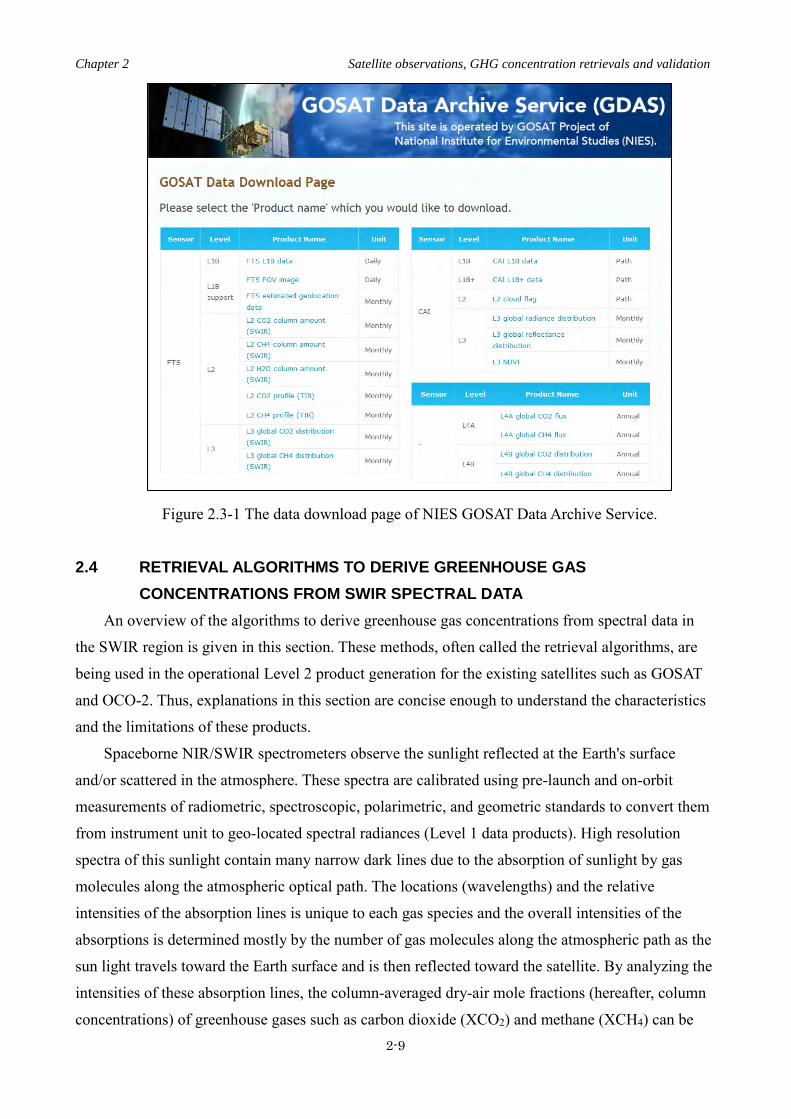
GOSAT standard products from Level 1 to 4 can be freely downloaded from NIES GOSAT
Data Archive Service (GDAS, https://data2.gosat.nies.go.jp/index_en.html, Figure 2.3-1). OCO-2
Level 1 and 2 products can be downloaded from NASA Goddard Earth Science Data & Information
Services Center (GES DISC, https://disc.gsfc.nasa.gov/datasets?page=1&keywords=OCO-2).
Additionally, GOSAT Level 2 data processed by different retrieval algorithms can be downloaded
from several sites such as European Space Agency's GHG-CCI
(http://www.esa-ghg-cci.org/sites/default/files/documents/public/documents/GHG-CCI_DATA.html
) and NASA's CO2 Virtual Science Data Environment (https://co2.jpl.nasa.gov).
Chapter 2 Satellite observations, GHG concentration retrievals and validation
2-9
Figure 2.3-1 The data download page of NIES GOSAT Data Archive Service.
2.4 RETRIEVAL ALGORITHMS TO DERIVE GREENHOUSE GAS CONCENTRATIONS FROM SWIR SPECTRAL DATA
An overview of the algorithms to derive greenhouse gas concentrations from spectral data in
the SWIR region is given in this section. These methods, often called the retrieval algorithms, are
being used in the operational Level 2 product generation for the existing satellites such as GOSAT
and OCO-2. Thus, explanations in this section are concise enough to understand the characteristics
and the limitations of these products.
Spaceborne NIR/SWIR spectrometers observe the sunlight reflected at the Earth's surface
and/or scattered in the atmosphere. These spectra are calibrated using pre-launch and on-orbit
measurements of radiometric, spectroscopic, polarimetric, and geometric standards to convert them
from instrument unit to geo-located spectral radiances (Level 1 data products). High resolution
spectra of this sunlight contain many narrow dark lines due to the absorption of sunlight by gas
molecules along the atmospheric optical path. The locations (wavelengths) and the relative
intensities of the absorption lines is unique to each gas species and the overall intensities of the
absorptions is determined mostly by the number of gas molecules along the atmospheric path as the
sun light travels toward the Earth surface and is then reflected toward the satellite. By analyzing the
intensities of these absorption lines, the column-averaged dry-air mole fractions (hereafter, column
concentrations) of greenhouse gases such as carbon dioxide (XCO2) and methane (XCH4) can be

Chapter 2 Satellite observations, GHG concentration retrievals and validation
2-10
derived. In case of GOSAT and OCO-2, absorption lines around 1.6 µm and 2.0 µm are used for
CO2 and CH4 measurements. Molecular oxygen (O2) absorption lines around 0.76 µm are also used
to estimate the surface air pressure and the column concentration of dry air along the same optical
path used to observe CO2 and CH4.
The observed NIR/SWIR spectra, however, are affected by not only the column concentrations
of greenhouse gases, but also other atmospheric constituents, land / ocean surface reflectance, and
instrumental parameters. Some of these properties are stable, but some are spatially and temporally
variable. To derive XCO2 and XCH4 from satellite data with the accuracy of about 0.25%, it is
necessary to estimate the environmental parameters simultaneously with XCO2 and XCH4. The
impact of the instrumental parameters is established through the calibration process.
To retrieve XCO2 or XCH4 from GOSAT and OCO-2 spectra, the observed spectrum is
simulated with a surface/atmospheric radiative transfer model using an assumed (a priori)
atmospheric and surface state. An inverse model based on optimal estimation (Rodgers, 2000) is
then used to update gas concentrations and other properties of the surface and atmospheric state to
minimize the difference between the observed and simulated spectra, and this process is repeated
until a good fit is achieved. Mathematical details of these algorithm can be found in O'Dell et al.
(2012), Yoshida et al. (2013), and the literature cited therein.
Scattering by clouds and aerosols (dust, haze, smog) can introduce uncertainties in the
atmospheric path length that can introduce errors in the XCO2 and XCH4 retrievals. To minimize
these errors, the optical properties and vertical distribution of atmospheric aerosols and clouds must
be retrieved simultaneously with the gas concentrations. Measurements acquired in the O2 A-band
at 0.76 µm provide insight into the cloud and aerosol scattering at that wavelength. However, an
accurate description of the wavelength dependent optical properties of clouds and aerosols is
needed to estimate their impact on the CO2 and CH4 bands at wavelengths near 1.61, 1.67, and 2.06
µm in the SWIR. Estimating these properties has been a major focus of the current researches, and
some users have adopted a "Proxy Method" that assumes that the scattering is the same in the
nearby CO2 and CH4 bands, so that if the concentration of one of these two gases is assumed to be
known, the other can be retrieved. For methane, see Schepers et al. (2012), Parker et al. (2015), and
the literature cited therein.
As most retrieval algorithms can successfully process only soundings with little or no cloud
contaminations within IFOV of their spectrometers, it is important to implement reliable cloud
detection and screening algorithms in the operational data processing system. Cloud information
can be derived from the SWIR reflectance spectra themselves. In the case of GOSAT, cloud maps
derived from a multispectral imager (Cloud and Aerosol Imager, CAI) are also used to detect cloud
fragments in the FTS IFOV. For OCO-2, clouds are screened using spectroscopic observations in
the O2 A-band and CO2 bands at 1.61 and 2.06 µm (see Taylor et al. 2011; 2016) or inferred from

Chapter 2 Satellite observations, GHG concentration retrievals and validation
2-11
co-located images.
Figure 2.4-1 shows the processing flow for GOSAT FTS SWIR Level 2 CO2 and CH4 data
products at NIES. GOSAT CAI Level 1B and Level 2 cloud flag processing is incorporated in this
figure as they provide cloud maps used in FTS Level 2 processing.
Figure 2.4-1 Processing Flow for FTS SWIR Level 2 CO2 and CH4 data products (Ver.02.2*) https://data2.gosat.nies.go.jp/doc/documents/DataProcessingFlow_FTSSWIRL2_V02.2x_en.pdf
2.5 VALIDATION OF COLUMN CONCENTRATIONS DERIVED FROM SATELLITE SWIR DATA
To ensure the accuracy of the XCO2 and XCH4 products derived from satellite data, the satellite
measurements must be accurately calibrated and the retrieved XCO2 and XCH4 estimates must be
validated against internationally-recognized standards. The instruments are calibrated both prior to
launch and then while in orbit to quantify the spectral, radiometric, and geometric performance.
Calibration is instrument specific and is not discussed further in this guidebook. To validate XCO2
and XCH4 estimates retrieved from satellite data (Level 2 or higher level products), these products
are quantitatively evaluated using the data with higher quality and independently measured by other
instruments. Here, the satellite data are often validated with ground-based and airborne in situ and
remote sensing measurements of these gases.

Chapter 2 Satellite observations, GHG concentration retrievals and validation
2-12
The validation approach for column concentrations derived from satellite SWIR spectral data
adopted by SCIAMACHY, GOSAT, and OCO-2 is to compare the XCO2 and XCH4 estimates
retrieved from the satellite data with the column concentrations derived from ground-based SWIR
spectral data collected by Total Carbon Column Observing Network (TCCON; Wunch et al. (2011)).
TCCON is a network of ground-based high resolution solar-viewing Fourier transform
spectrometers (FTS) deployed over a range of latitudes and longitudes (Figure 2.5-1).
Figure 2.5-1. Locations of TCCON sites.
(http://tccondata.org/img/tccon_map.jpg)

Chapter 2 Satellite observations, GHG concentration retrievals and validation
2-13
Figure 2.5-2. GOSAT FTS Level 2 products (Version 2) validation results with TCCON data:
(left) XCO2 and (right) XCH4
(http://www.gosat.nies.go.jp/eng/gosat_leaflet_en.pdf)
For detailed results of GOSAT and OCO-2 validation activities, see Morino et al. (2011) and
Yoshida et al. (2013) for GOSAT and Wunch et al. (2017) for OCO-2. According to Yoshida et al.
(2013), the biases and the standard deviations of the GOSAT Level 2 products V02.00 are -1.48 and
2.09 ppm for XCO2 and -5.9 and 12.6 ppb for XCH4, respectively (Figure 2.5-2). According to
Wunch et al. (2017), the absolute median differences and the RMS differences of OCO-2 XCO2 are
less than 0.4 ppm and less than 1.5 ppm, respectively. These values are interpreted as the accuracy
and precision of the XCO2 and XCH4 satellite data. Biases in the retrieved concentration data can be
reduced by empirical methods (e. g. Inoue et al., 2016) or through comparisons with outputs from
atmospheric transfer models which calculate global gas concentration distribution.

Chapter 3 Using satellite observations for emission estimates and comparison to inventories
3-1
3. SATELLITE OBSERVATIONS AND DATA APPLICATIONS, PART 2: USING SATELLITE OBSERVATIONS FOR EMISSION ESTIMATES AND COMPARISON TO EMISSION INVENTORIES Introduction
Atmospheric measurements of GHGs can provide a useful additional constraint on emissions
where bottom-up inventories are incomplete or inaccurate (Henne et al., 2016; Saunois et al., 2016).
A number of techniques are employed for estimating fluxes from GHG concentration measurements.
On the smallest scales, a mass balance approach can be used to estimate fluxes from concentration
measurements collected upwind and downwind of a known emission source, with surface and
airborne measurement campaigns (Karion et al., 2011; McKain et al., 2015; Zavala-Araiza at al.,
2015). On larger scales, ranging from city to national and continental scale, inverse models of
atmospheric transport and other methods, including inter-tracer correlation, are used to estimate the
surface fluxes. Inverse models use an atmospheric tracer transport model to simulate GHG
concentration at observation locations given some assumed surface fluxes. Surface flux
optimization techniques are applied to provide the best fit between observed concentrations and
simulations with an atmospheric transport model (Enting, 2002).
Similarly to ground based measurements, use of the satellite observations for anthropogenic
GHG emission estimates can be divided into two approaches. Mass balance approaches are
described in section 3.1, and inverse models are described in section 3.2.
3.1 Emission estimates based on analysis of concentration anomalies around emission sources
While ground-based in situ measurements can provide estimates of GHG concentrations at the
surface that are both precise and accurate, these measurements are spatially sparse and often
provide no information about atmospheric profile of these gases. In contrast, space based remote
sensing observations provide estimates of the column-averaged GHG concentration with much
greater spatial resolution and coverage, but these estimates are often less precise and accurate as the
ground-based in situ measurements.
Accordingly, some emission estimate methods, that can be used successfully with ground based
observations, are not directly applicable to satellite observations due to lower precision of the
satellite retrievals and due to observing vertically integrated concentration, which dilutes sensitivity
to GHG concentrations in the planetary boundary layer. In the cases where the GHG concentration
gradients are small, the lower precision of the space based measurements can be compensated to
some extent by accumulating a large number of lower precision measurements. This approach can
be applied over an extended period of time to recover information about the long-term mean
Chapter 3 Using satellite observations for emission estimates and comparison to inventories
3-2
concentration differences between clean regional background and observations made directly over
the emission point and its plume (Schneising et al., 2008, 2011; Kort et al., 2012; Janardanan et al.,
2016, 2017; Hakkarainen et al., 2016; Turner et al., 2016; Buchwitz et al., 2017 and others).
Notably, some OCO-2 observations of power plant plumes (Nassar et al., 2017) can be analyzed to
yield flux estimates without long-term averaging on an event basis, due to lower single sounding
random errors and its smaller surface footprint allowing observations of narrow plumes of high CO2
concentration.
A number of emission estimation methods relying on observations of the concentration
enhancements around emission sources and their temporal trends have been developed over the past
decade. Anthropogenic emissions of CO2, CH4, as well as NOx, CO and other pollutants lead to
buildup of the emitted tracers above the emission area and the transport of a high concentration
plume downstream of the emission source (city, powerplant, etc.) by wind. Satellites observe
increased column GHG concentration when the plume is in their observation footprint. The
emission plumes or enhancements can be identified either by:
(1) long term averaging of the observed concentration (Schneising et al., 2008, 2011, 2014a;
Buchwitz, et al., 2017),
(2) comparing with model simulations (Janardanan et al., 2016, 2017; Nassar et al., 2017), or
(3) by collocated observation of another pollution tracer such as NO2 by OMI (Hakkarainen et
al., 2016) and NH3 by GOSAT TIR (Ross et al., 2013), or transport model simulation of pollution
tracer CO (Parker et al., 2016).
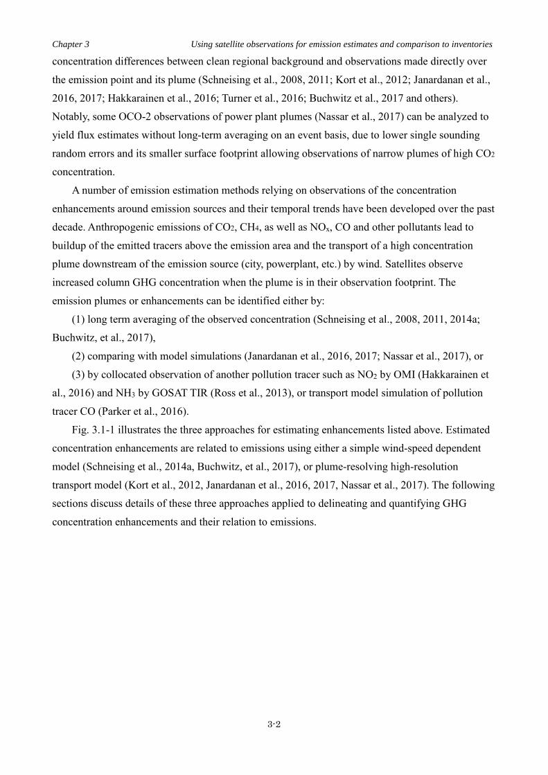
Fig. 3.1-1 illustrates the three approaches for estimating enhancements listed above. Estimated
concentration enhancements are related to emissions using either a simple wind-speed dependent
model (Schneising et al., 2014a, Buchwitz, et al., 2017), or plume-resolving high-resolution
transport model (Kort et al., 2012, Janardanan et al., 2016, 2017, Nassar et al., 2017). The following
sections discuss details of these three approaches applied to delineating and quantifying GHG
concentration enhancements and their relation to emissions.

Chapter 3 Using satellite observations for emission estimates and comparison to inventories
3-3
Fig. 3.1-1 Diagram showing three approaches to extracting XCO2 anomalies from multiyear
time series of satellite observations: (a) long term averaging of SCIAMACHY data over Western
Europe, from (Scheising et al., 2008); (b) GOSAT observation locations (in red) used to simulate
XCO2 using high resolution transport model and CO2 emissions (in grey), as in Janardanan et al.,
(2016); (c) OMI observations of NO2, that provide information on “polluted” vs “clean” air for
filtering OCO-2 observations (Hakkarainen et al., 2016).
3.1.1 Long-term averaging As found by Schneising et al., (2008) when analyzing SCIAMACHY XCO2 retrievals for a
period of 3 years (2003-2005), both the measurement noise and the noise introduced as the CO2
from other sources is transported over the source of interest by the winds is suppressed by
averaging, and local concentration anomalies become visible, coinciding geographically with areas
of strong surface emissions. Long term averages of SCIAMACHY measurements of methane were
even able to detect trends in local concentration anomalies over emitting areas (Schneising et al.,
2014a).
Applying long-term averaging is a convenient way to extract emission-related concentration
anomalies, as it doesn’t require transport modeling or a proxy tracer observation. However, the
quantitative value of the derived anomalies for the emission estimates is limited, as averaging sums
up the enhancements due to emission contributions from different wind directions and at different
wind speeds. Long-term averaging was shown to work for sensors like SCIAMACHY or OMI,
which provide coarse wide swath observations, resulting in almost continuous observation coverage.
In the case of narrow swath instruments, like OCO-2, or coarse footprint sampling observations, as
in the case of GOSAT, a modified approach to long-term averaging will be needed.
3.1.2 High resolution transport modeling
Janardanan et al., (2016, 2017), and Heymann et al., (2017) used high resolution transport
models to simulate each GHG plume transported by wind from strong emission sources, while
Nassar et al., (2017) used simple Gaussian plume model for this purpose. In addition to filtering the
observations by threshold value of simulated enhancements, Janardanan et al. (2016, 2017) applied
binned averaging of the observed enhancements that resulted in a large reduction in observation

Chapter 3 Using satellite observations for emission estimates and comparison to inventories
3-4
noise, making the relationship between modeled and observed enhancements visibly close to linear.
In this approach, a simple ratio of the mean observed to simulated enhancements or a regression
slope value is used as a correction factor for adjusting the emission intensities provided by an
emission inventory to match the observed concentrations.
Using transport modeling has the merit of allowing both extraction of the concentration
anomalies and taking wind speed into account when relating the concentration anomalies to surface
emissions. However, there are also multiple difficulties of applying the local scale transport
modeling, including:
(1) uncertainties related to defining a clean background;
(2) a need for accurate high resolution wind data, resolving coastal air circulations and
topographic effects;
(3) correlated errors due to aerosol loading leading to retrieval biases.
3.1.3 Use of the collocated observations of another tracer of atmospheric pollution Use of high resolution transport modeling in backward transport mode (Janardanan et al., 2016,
2017) requires a large volume of computations in cases of satellite instruments that produce a large
amount of data (like OCO-2). In that case, collocated observations of another tracer can be applied
to detect the observations influenced by GHG emissions and separate them from observations made
in the clean air.
In Nassar et al. (2017), OCO-2 observations from direct overpasses or close flybys of
individual coal-burning power plants were fit to simulations using a vertically-integrated Gaussian
plume model. This required conversion of the OCO-2 observations to XCO2 enhancements relative
to the background and converting plume model enhancements from gC/m2 to ppm. Although the
approach avoids simple averaging of the data so that it can utilize gradients within the emission
plume, each emission estimate was based on from 17 to 167 (mean of 66) OCO-2 footprints from
the plume and larger numbers for the background (126-489, mean of 310). An associated method
for quantifying emission estimate uncertainties accounts for the impact of wind speed uncertainty,
background uncertainties, observation enhancement uncertainties and potential interfering emission
sources. More details on this study are given in the case study section of the Guidebook.
Hakkarainen et al. (2016) constructed CO2 anomaly maps from OCO-2 data, and then used
NO2 observations from OMI to determine whether these anomalies were correlated with fossil fuel
or biomass burning sources. Ross et al. (2013) used GOSAT TIR NH3 observations to identify
surface GOSAT footprints influenced by biomass burning, and proceeded with using the data for
deriving the ratio of CH4 to CO2 emissions by biomass burning. Parker et al. (2016) used
simulations of CO transport driven by biomass burning emissions to detect influences of biomass
burning in GOSAT footprints, also for deriving ratio of CH4 to CO2 emissions.

Chapter 3 Using satellite observations for emission estimates and comparison to inventories
3-5
Using a reference tracer of atmospheric pollution was shown to be sometimes more accurate
than high resolution transport modeling for discriminating between polluted versus clean
background air (Oney et al., 2017). Limitations are also present: (1) although the method is good for
extracting anomalies related to combustion, other processes (fugitive emissions of methane)
correlate to combustion intensity (NO2, CO) only at much larger scales; (2) the emission estimates
depend on uncertainty of the reference tracer emissions, and accounting for chemical transformation
of the reference tracer.
3.2 Anthropogenic GHG emission estimates based on inverse modeling Inverse models combine information about the atmospheric transport with observations of
GHG concentrations, and adjust the surface fluxes to produce a good fit of the transport model
simulation to the observations. Inverse models have been used along with ground based GHG
observations to regional and national scale anthropogenic non-CO2 GHG emission estimates (Stohl
et al., 2009; Manning et al., 2011; Miller et al., 2013; Henne et al., 2016 and others) and city-scale
CO2 emissions (Brioude et al., 2013; Breon et al., 2015; Lauvaux, et al., 2016). In flux inversion
experiments that use sparse, but accurate surface GHG measurements, the number of observations
is critical as the strength of the observational constraint for estimated fluxes is proportional to the
number of available observations and inversely proportional to the uncertainty of a single
observation (Enting, 2002). Thus, as pointed out by Rayner and O’Brien, (2001), satellite
observations available in large volume over regions underrepresented by the surface network are
useful for surface flux estimates, even when taken with a precision lower than that of the ground
based observations. Inverse modeling techniques that were developed for estimating surface fluxes
with ground-based observations (Rayner et al., 1999; Rodenbeck et al., 2003) are being applied to
satellite observations as well (Meirink et al., 2008; Maksyutov et al., 2013; Houweling et al., 2015;
Turner et al., 2015 and others). There are also several reviews of methods which have been tested
and applied to use of the GHG concentration observations for emission estimates at local and
regional scale (Jacob et al., 2016, Streets et al., 2013).
An inverse model relies on an atmospheric transport model to simulate the concentrations of
emitted tracers at the observation locations with emission intensity fields, and tries to find a surface
emission field that provides a best match between simulated and observed data. Due to the limited
spatial and temporal resolution of the winds and other limitations of the atmospheric transport
models, the mismatch between observed and optimized data can be larger than the GHG
measurement errors.
A brief outline of the inverse modeling approach as mathematical formulation of the flux
optimization problem is given in Section 4.6.2 of this Guidebook, while more detailed description
that can be found in (Enting, 2002) and other introductory texts on inverse modeling.

Chapter 3 Using satellite observations for emission estimates and comparison to inventories
3-6
Depending on observation data available for constraining the target flux category, the
uncertainties of the inverse model estimates can be larger than those of inventory, as it is often the
case for anthropogenic CO2 emissions, thus application of the inverse modeling is only justified
when the uncertainty of the inventory is larger or comparable to the uncertainty of the inverse
model estimates. The uncertainties of anthropogenic emission inventories vary widely depending on
target tracer, region, country and source category. There are also difficulties in estimating the
uncertainty of the bottom-up inventory. One example of significant discrepancies between emission
inventories and inverse model estimates is related to recent US emissions in the oil and gas category
(Miller and Michalak, 2017). The main difficulty leading to uncertainty of the emission inventory
for some species is large variability of the emission factors. As Beusse et al., (2014) mentioned, the
uncertainty of methane emissions factors for US gas pipelines estimated by US Environment
Protection Agency (EPA) study was 65%. For CO2, the uncertainty of anthropogenic annual CO2
emission inventories is rather low at the country scale in most cases (Rypdal et al., 2005), however,
it can still be high for emerging economies which now represent some of the highest emitting
nations and a larger share of global CO2 emissions. Furthermore, CO2 emission uncertainties are
larger for smaller space and time scales, which makes top-down estimates less relevant for national
reporting, but more relevant for the implementation of NDCs and for countries to understand the
effectiveness of their efforts to achieve their NDCs and track their own progress.
3.2.1 Application of the inverse model emission estimates for comparison with national
inventories Use of satellite observations in inversion is in the experimental stage, due to multiple technical
challenges of producing the high-quality concentration retrievals from the satellite-observed spectra.
However, there are several promising results. A number of methane inverse modeling studies were
conducted using (mostly) GOSAT and SCIAMACHY satellite data (Fraser et al., 2013; Alexe et al.,
2015; Pandey et al., 2017; Turner et al., 2015; Cressot et al., 2014) and several of those have been
intercompared in a Global Carbon Project CH4 (GCP-CH4) study by Saunois et al., (2016). A
valuable outcome of the comparisons performed by Saunois et al., (2016), Bruhwiler et al., (2017)
and Cressot et al. (2014) is that they have shown a general consistency between ground-based data
inversions and satellite-based data inversions in terms of the estimated emissions for important
emission regions such as East Asia and North America. The GCP-CH4 study results for 2012 show
that the spread (standard deviation) of anthropogenic methane emissions estimates between
different inverse models for large regions (temperate North America, boreal North America, Europe,
Central Asia and Japan, China, Russia) is between 11 to 25 % of the multi-model average for each
region, and GOSAT-based estimates are within the range of the estimates. Accordingly, the inverse
model estimates based on space-based observations can be considered as an additional source of
Chapter 3 Using satellite observations for emission estimates and comparison to inventories
3-7
data for national inventory comparisons alongside with estimates based on surface observation data.
It should be noted that inverse models have biases dependent on design of the transport model,
and the emission estimates are sensitive to underlying transport model biases. The differences are
apparent when estimates for the same region and time period are compared (Houweling et al., 2015;
Saunois et al., 2016). On the other hand, the differences become smaller when interannual flux
variability and temporal trends are concerned, as shown recently by analysing the trends in methane
emission estimates by several inverse models included in the GCP-CH4 study for North America
(Bruhwiler et al., 2017). Patra et al., (2016) and Saeki and Patra, (2017) applied inverse modeling of
CH4 and CO2 fluxes over East Asia for checking the inventory time series consistency. Patra et al.,
(2016) concluded that the growth rate in East Asian emissions of CH4 was likely to be
overestimated by bottom-up inventories.
Publicly available inverse model estimates for CH4 emissions based on satellite and
ground-based measurements are provided by inverse model products, including the global inversion
product from the Copernicus Atmospheric Monitoring Service1 (CAMS), (Bergamaschi et al., 2013),
NASA CMS-flux product for North America, (Turner and Jacob, 2016) and GOSAT Level 4A
product (CH4) (Saito et al., 2016). Several institutions, such as Laboratoire des Sciences du Climat
et de l'Environnement (LSCE), Max Planck Institute for Biogeochemistry (MPI BGC), Harvard
University and others also make their emission estimates at the global scale based on satellite data
and make their gridded flux data available upon request.
Although the satellite-based global products are currently provided at coarse resolution (2-3
degrees), an upgrade to higher resolution is foreseen, based on recently developed regional zoom
approaches, like those based on the NAME model (Ganesan et al., 2017; Manning et al., 2011),
CHIMERE (Broquet et al., 2011) or Carbontracker-Lagrange (He et al, 2017).
To compare national inventory to publicly available inverse modeling products introduced
above, one should implement following steps:
1. Check if the inverse modeling product confirms to at least 3 criteria:
(1) the product is checked for probable errors and inconsistencies via comparison to other
inverse modeling estimates (see Saunois et al., 2016, Bruhwiler et al., 2017);
(2) observations impose strong enough constraint on estimated fluxes, the inverse model uses
several observation sites over the country and, possibly, good satellite data coverage,
sufficient to reduce flux uncertainty by 30-50%;
(3) the estimated inverse model flux uncertainty is less than uncertainty of the national
inventory.
2. Based on the inverse modelling data available at the time of inventory report preparation,
select available time periods overlapping between inventory data and inverse model results.
Download gridded emission data files, file format descriptions and release notes.

Chapter 3 Using satellite observations for emission estimates and comparison to inventories
3-8
3. Remapping from gridded data to country boundaries. Calculate area fraction of the national
land area in each grid cell of the emission data grid (fractional overlap between data grid cell
boundaries and nation borders). Use area fraction to calculate national total emission for
each time period (usually available at monthly time step), by summing grid emissions
multiplied by fraction of national land area. Derive national total for each year by summing
the monthly total emissions.
4. Remap emission uncertainty, in the case all the data required for regional emission
uncertainty estimates is provided together with inverse modelling results.
5. When the number of available inverse modelling products is greater than one, remap to
national total for each year for all the available products. It is useful to include in the
comparison national total estimates with each available inverse modelling product, as in
(Bergamaschi et al., 2018).
The above step-by-step guidance is illustrated in the following diagram (Fig. 3.2-1)
Fig. 3.2-1 Step by step procedure for extracting the national (reginal) total emissions from inverse
modeling products.
Ready-made estimates for several countries, such as US (conterminous), Russia and China for
year 2012 are prepared based on Global Carbon Project CH4 inverse model estimates (Saunois et al.
2016) using a procedure that is described above and are published on the Environmental System
Science Data Infrastructure for a Virtual Ecosystem (ESS-DIVE) web site (Global Methane Budget
2000-2012, 2016).
Useful examples of comparison between national emissions estimated by inventory and inverse

Chapter 3 Using satellite observations for emission estimates and comparison to inventories
3-9
model are given by Bruhwiler et al. (2017) and Turner et al. (2015), both made for USA. Separate
estimates of the sector-specific anthropogenic (oil and gas, agriculture and waste) and natural
(wetlands) emissions is still a problem even for recent high resolution regional inverse modeling
studies (Bergamaschi et al., 2018). Nevertheless, Turner et al. (2015) used GOSAT observations and
a transport model with high resolution zooming over North America to project likely
underestimation of the anthropogenic emissions in US methane emission inventory. In their case,
distinguishing between natural and anthropogenic sources is assisted by geographical separation
between natural sources (wetlands in the North) and growing oil and gas emissions in the South.
More details on the study by Turner et al. (2015) are also given in the case study section 4.6 of this
Guidebook. An estimate of the Indian national total emissions of methane was made by Ganesan et
al., (2017) using high resolution regional inverse model and combination of the ground based
observations and GOSAT data. They have concluded that atmospheric observation data support the
nationally reported emissions in terms of both trend and amount.
1 http://atmosphere.copernicus.eu/documentation-supplementary-products#greengas-fluxes

Chapter 4 Case Studies
4.0-1
4. CASE STUDIES In this chapter, several case studies in which greenhouse gas inventories are compared with the
estimates from satellite-based or ground-based concentration measurements are described. Target
gases, gas concentration data sources, and methods in each section are summarized in Table 4.0-1.
Table 4.0-1. Summary of case studies in Chapter 4.
Section Target gas Gas concentration data source Method
4-1 CO2 SCIAMACHY Concentration enhancement
4-2 CO2 OCO-2 Concentration enhancement
4-3 CO2 and CH4 GOSAT and SCIAMACHY Concentration enhancement
4-4 CO2 and CH4 GOSAT Concentration enhancement
4-5 CH4 GOSAT and SCIAMACHY Concentration enhancement
4-6 CH4 GOSAT Inverse modeling
4-7 CO2 GLOVALVIEW (flask) Inverse modeling
4-8 CH4 WDCGG and GOSAT Inverse modeling
4-9 CO2 OCO-2 Concentration enhancement

Chapter 4 Case Studies
4.1-1
4.1 Anthropogenic CO2 emission trends from SCIAMACHY/ENVISAT and comparison with EDGAR M. Buchwitz1, M. Reuter1, O. Schneising-Weigel1, H. Bovensmann1, and J. P. Burrows1
1) Institute of Environmental Physics (IUP), University of Bremen, Germany
4.1.1 Introduction
SCanning Imaging Absorption spectroMeter for Atmospheric CHartographY (SCIAMACHY)
(Burrows et al., 1995; Bovensmann et al., 1999) onboard of the European environmental satellite
ENVISAT was operational from March 2002 to April 2012. SCIAMACHY was a passive remote
sensing spectrometer observing backscattered, reflected, transmitted or emitted radiation from the
atmosphere and Earth's surface, in the wavelength range between 240 and 2380 nm. The spatial
resolution depends on spectral region but was typically 30 km along track and 60 km across track.
Global coverage at the equator was achieved after six days (swath width 960 km; nominal
measurement sequence: 50% nadir (downlooking) and 50% limb (scanning the atmosphere while
looking to the Earth’s horizon and above)).
For the retrieval of column-averaged dry-air mole fractions of carbon dioxide (CO2), i.e., XCO2,
two spectral regions have been used: the 1.6 μm region containing CO2 absorption lines and the
0.76 μm spectral region covering the oxygen (O2) A-band.
The retrieved XCO2 (e.g., Buchwitz et al., 2000, 2015, 2016; Schneising et al., 2008, 2011;
Reuter et al., 2010, 2011; Heymann et al, 2015) has been used to address important scientific issues
related to the natural sources and sinks of atmospheric CO2 (e.g., Reuter et al., 2014a, 2017;
Schneising et al., 2014b).
In the following results from studies related to anthropogenic CO2 emissions, which have been
published in the peer-reviewed scientific literature (Schneising et al., 2008, 2013; Reuter et al.,
2014b), are summarized.
4.1.2 Data 4.1.2.1 GHG Concentration Data
Schneising et al., 2008, analyzed SCIAMACHY year 2003-2005 XCO2 retrievals. For
validation the XCO2 product of the Total Carbon Column Observing Network (TCCON) (Wunch et
al., 2011) has been used. Furthermore, they used atmospheric CO2 fields from NOAA’s
CO2-assimilation system CarbonTracker (Peters et al., 2007).
Schneising et al., 2013, used SCIAMACHY XCO2 retrievals covering the time period
2003-2009 and CarbonTracker CO2 fields (Peters et al., 2007).
Reuter et al., 2014b, used SCIAMACHY XCO2 retrievals from the time period 2003-2011.

Chapter 4 Case Studies
4.1-2
4.1.2.2 Other Data
Schneising et al., 2008, used for comparison with the satellite XCO2 retrievals population
density (CIESIN/CIAT, 2005) and EDGAR anthropogenic CO2 emissions (EDGAR 3.2 Fast Track
2000 dataset (32FT2000), Olivier et al., 2005). Furthermore, MODIS/Terra aerosol optical depth
has been used (Level 3 collection 5 product obtained from http://modis-atmos.gsfc.nasa.gov/) and
subvisual cirrus cloud retrievals from E. Martins, LMD/IPSL, Palaiseau, France.
Schneising et al., 2013, used for comparison EDGAR anthropogenic CO2 emissions (version
4.2, Olivier et al., 2012). In addition, an aerosol optical depth data set based on MODIS from the
European GEMS (Global and regional Earth-system Monitoring using Satellite and in-situ data)
project has been used (obtained from http://data-portal.ecmwf.int/data/d/gems reanalysis/).
EDGAR version 4.2 has also been used by Reuter et al., 2014b. In addition, SCIAMACHY
NO2 vertical column retrievals have been used.
4.1.3 Methods 4.1.3.1 Outline
Different methods have been used in each of the three publications. These methods are shortly
described in the following sub-sections.
4.1.3.2 Methodology used by Schneising et al., 2008
The main goal of Schneising et al., 2008, was to demonstrate that regionally elevated CO2 over
major anthropogenic source regions can be detected from space. Focus was on the Rhine-Ruhr area
in western central Europe but other regions have also been studied, e.g., the US East Coast and the
region around Tokyo in Japan. To eliminate XCO2 variations not originating from anthropogenic
CO2 emissions, in particular variations due to uptake and release of CO2 by the terrestrial biosphere,
and to reduce noise, the satellite XCO2 retrievals have been averaged over all three years
(2003-2005) using a spatial grid of 0.5ox0.5o. The resulting XCO2 maps have been compared with
population density and EDGAR anthropogenic CO2 emissions. In order to make sure that the
observed elevated satellite-derived XCO2 is not significantly affect by aerosols or thin clouds,
satellite aerosol optical depth and information on subvisual cirrus clouds have been used. In
addition, also simulated retrievals have been carried out as part of the error analysis. For details
please see Schneising et al., 2008.
4.1.3.3 Methodology used by Schneising et al, 2013 The method used by Schneising et al., 2013, is similar as the method used by Schneising et al.,
2008. The main differences are (i) the use of a longer time period, (ii) the aim to obtain information
on emission trends, and (iii) to achieve a more quantitative comparison with EDGAR anthropogenic

Chapter 4 Case Studies
4.1-3
CO2 emissions assuming that a regional relative CO2 emission enhancement corresponds to the
same relative regional XCO2 enhancement over the source region of interest. For details please see
Schneising et al., 2013.
4.1.3.4 Methodology used by Reuter et al, 2014b The method of Reuter et al., 2014b, differs significantly from the methods of Schneising et al.,
2008 and 2013. Reuter et al., 2014b, took advantage of the fact that SCIAMACHY provides
retrievals of NO2 vertical columns in addition to XCO2. They used satellite-derived NO2 as a tracer
for anthropogenic emissions and calculated regional anomalies ΔXCO2 and ΔNO2 from collocated
SCIAMACHY XCO2 and NO2 retrievals. They found an approximately linear relationship between
satellite-derived ΔXCO2 and ΔNO2 and interpreted the slope as a (regionally dependent) conversion
factor allowing the use of NO2 as a proxy for expected regional XCO2 enhancements from nearby
anthropogenic emissions (“XCO2e”). XCO2
e is an estimate of the expectation value of the XCO2
enhancement resulting from the source (or sources) causing a measured NO2 level. Using this
method, they obtained emission trends and CO2-to-NOx emission ratios, which were compared with
EDGAR. A very detailed error analysis is also presented in Reuter et al., 2014b, which had been
carried out in order to obtain reliable uncertainty estimates. For details please see Reuter et al.,
2014b.
4.1.4 Case Study Results In the following three sub-sections the main results from the three case studies are shortly
presented and summarized.
4.1.4.1 Results obtained by Schneising et al., 2008
The main goal of the study of Schneising et al., 2008, was to find out if regionally elevated CO2
over major anthropogenic source regions can be detected from space. Their results can be
summarized follows: When averaging the SCIAMACHY XCO2 retrievals over the time period
2003-2005 the resulting map for western central Europe (Fig. 4.1-1) shows elevated CO2 over the
highly populated region of western central Germany and parts of the Netherlands and Belgium
(“Rhine-Ruhr area”). They found that the spatial pattern is reasonably well correlated with
population density and EDGAR anthropogenic CO2 emissions (see Fig. 4.1-2). Note that a perfect
correlation cannot be expected due to atmospheric transport and sparse sampling of the satellite data.
On average they found a regional enhancement of 2.7 ppm over this region (XCO2 average in red
rectangle minus green rectangle in Fig. 4.1-2). The potential contribution to this enhancement from
regionally elevated aerosols and sparse sampling of the satellite data was conservatively estimated
to 1-1.5 ppm. They found similar results also for other major anthropogenic source regions such as

Chapter 4 Case Studies
4.1-4
the US East Coast and the region around Tokyo in Japan. Overall, they concluded that their findings
indicate that regionally elevated CO2 arising from regional anthropogenic CO2 emissions can
potentially be detected from space.
Figure 4.1-1. Elevated CO2 over western central Europe’s major anthropogenic source region, the
Rhine-Ruhr area, covering parts of Germany, the Netherlands and Belgium. Adapted from
Schneising et al., 2008 (see Fig. 4.1-2 for their original figure).
4.1.4.2 Results obtained by Schneising et al., 2013 The main goal of the study of Schneising et al., 2013, was to obtain more quantitative results
compared to the predecessor study presented in Schneising et al., 2008. A summary of their main
results is shown in Fig. 4.1-3. By subtracting satellite retrieved XCO2 background values from those
retrieved over urban areas significant CO2 enhancements for several anthropogenic source regions
have been found, namely 1.3±0.7 ppm for the Rhine-Ruhr metropolitan region and the Benelux,
1.1±0.5 ppm for the East Coast of the United States, and 2.4±0.9 ppm for the Yangtze River Delta
area in China. The order of magnitude of the enhancements is in agreement with what is expected
for anthropogenic CO2 signals. The larger standard deviation of the retrieved Yangtze River Delta
enhancement is due to a distinct positive trend of 0.3±0.2 ppm/yr, which is quantitatively consistent
with anthropogenic emissions from the Emission Database for Global Atmospheric Research
(EDGAR) in terms of percentage increase per year (see Fig. 4.1-3 bottom right). The obtained
trends over Central Europe and the US East Coast also agree with EDGAR within the (quite large)
uncertainty of the satellite-derived trends.

Chapter 4 Case Studies
4.1-5
Figure 4.1-2. Top: SCIAMACHY XCO2 during 2003-2005 over western Central Europe. Middle:
Population density. Bottom: EDGAR anthropogenic CO2 emissions. From Schneising et al., 2008
(their Fig. 17).
4.1.4.3 Results obtained by Reuter et al., 2014b
Reuter et al., 2014b, analyzed simultaneous and co-located satellite retrievals from
SCIAMACHY of the column-average dry-air mole fraction of CO2, i.e., XCO2, and NO2 vertical
columns for the years 2003–2011 to provide top-down estimates of emission trends and CO2 to
NOx emission ratios. Their analysis (Figs. 4.1-3 and 4.1-4) showed that the CO2-to-NOx emission
ratio has increased by 4.2+/-1.7%/yr in East Asia. In this region, they found a large positive trend of
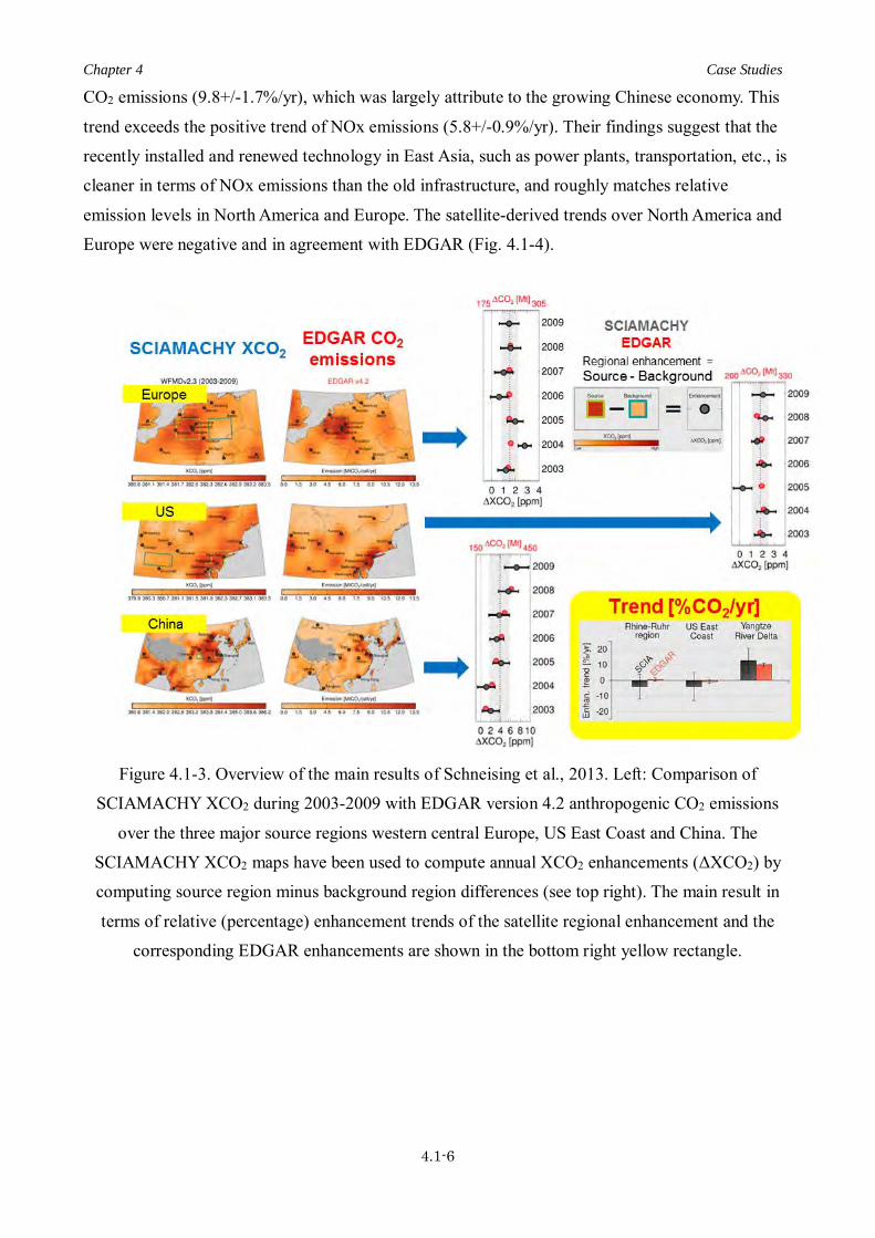
Chapter 4 Case Studies
4.1-6
CO2 emissions (9.8+/-1.7%/yr), which was largely attribute to the growing Chinese economy. This
trend exceeds the positive trend of NOx emissions (5.8+/-0.9%/yr). Their findings suggest that the
recently installed and renewed technology in East Asia, such as power plants, transportation, etc., is
cleaner in terms of NOx emissions than the old infrastructure, and roughly matches relative
emission levels in North America and Europe. The satellite-derived trends over North America and
Europe were negative and in agreement with EDGAR (Fig. 4.1-4).
Figure 4.1-3. Overview of the main results of Schneising et al., 2013. Left: Comparison of
SCIAMACHY XCO2 during 2003-2009 with EDGAR version 4.2 anthropogenic CO2 emissions
over the three major source regions western central Europe, US East Coast and China. The
SCIAMACHY XCO2 maps have been used to compute annual XCO2 enhancements (ΔXCO2) by
computing source region minus background region differences (see top right). The main result in
terms of relative (percentage) enhancement trends of the satellite regional enhancement and the
corresponding EDGAR enhancements are shown in the bottom right yellow rectangle.

Chapter 4 Case Studies
4.1-7
Figure 4.1-4. Overview of the main results of Reuter et al., 2014b. The maps show SCIAMACHY
NO2 converted to XCO2 using regionally dependent conversion factors obtained from co-located
SCIAMACHY XCO2 and NO2 column correlations and a filtering method to select ground pixels
affected by near-by anthropogenic sources. The histograms show derived emission trends for NOx
(red) and CO2 (green) over the source regions North America / Europe (left) and East Asia (right).
Adapted from Reuter et al., 2014b (see Fig. 4.1-5 for the original figure).
Figure 4.1-5. Trends of CO2-to-NOx emission ratios (grey), tropospheric NO2 emissions (red),
XCO2 enhancements (green) and corresponding emission trends from EDGAR (green-white
striped). From Reuter et al., 2014b (their Fig. 3). For details see Reuter et al., 2014b.

Chapter 4 Case Studies
4.2-1
4.2 Direct space-based Observations of Anthropogenic CO2 Emission Areas: Global XCO2 Anomalies Janne Hakkarainen1, Iolanda Ialongo1, and Johanna Tamminen1
1) Finnish Meteorological Institute, Earth Observation, Helsinki, Finland
4.2.1 Introduction
Over the past two decades, spaceborne measurements of short-lived air pollutants (such as
nitrogen dioxide NO2 and sulfur dioxide SO2) have revolutionized the way we monitor atmospheric
composition, providing more and more accurate information on the pollution levels on the global
scale. In comparison to these short-lived air pollutants that are detected close to the emission
sources, the growing trend, strong seasonality, long lifetime, and large atmospheric background,
significantly complicate the analysis of the anthropogenic CO2 emissions from space. This is why
most studies employ auxiliary data from models, emission inventories, or other proxies in order to
identify anthropogenic CO2 emission areas from satellite-based CO2 columns.
Direct methods, i.e. methods that are based on direct usage of space-based observations and not
on atmospheric modeling, have proven to have several desirable properties for example in air
quality applications. For example direct methods can reveal discrepancies between emission
inventories and identify missing sources, as seen e.g. for NO2 and SO2 [McLinden et al., 2016] and
for methane [Kort et al., 2014]. Superior spatial detail can also be reached from space-based
observations, as many inversion methods are based on scaling pre-described a priori fields. A great
challenge in direct methods, however, is to translate concentration information to emissions.
This section summarizes a recent study [Hakkarainen et al., 2016] that presents a direct
observation of anthropogenic CO2 from Orbiting Carbon Observatory-2 (OCO-2). The study
proposes a novel methodology to detect anthropogenic CO2 emission areas, solely based on
spaceborne CO2 measurements. The fundamental idea is to average-out the CO2 transport and
calculate long-term averages of CO2 anomalies. These anomalies are obtained by deseasonalizing
and detrending the data. The key is to use the observations themselves by removing the regional
daily median values. For comparison, OMI (Ozone Monitoring Instrument) NO2 tropospheric
columns are used as an independent tracer of atmospheric pollution and CO2 and NO2 information
are combined via cluster analysis. The results are also compared with existing anthropogenic CO2
emission inventories.
4.2.2 Data The column-averaged dry air mole fraction of CO2 (XCO2) data from Orbiting Carbon
Observatory-2 (OCO-2) are used in the analysis. The methodology is also applicable to the
Greenhouse gases Observing SATellite (GOSAT) data, and this option will be exploited in more

Chapter 4 Case Studies
4.2-2
detail in future studies.
4.2.2.1 OCO-2 Data Recently, measurements of column-averaged dry air mole fraction of CO2 (XCO2) have
become available from the Orbiting Carbon Observatory-2 (OCO-2) [Crisp et al., 2004]. The
instrument provides measurements with eight 2.25 km long footprints along a narrow (0.4 to 1.29
km) swath [Crisp et al., 2008]. The ACOS (Atmospheric CO2 Observations from Space) retrieval
algorithm is used to derive XCO2 [O'Dell et al., 2012]. The study uses the version 7 reprocessed lite
files including bias corrected XCO2 data available from September 2014 to April 2016. The data
have been screened using quality flags set to zero and warning levels smaller than 15.
4.2.2.2 Auxiliary Data The NO2 tropospheric column measurements from the Ozone Monitoring Instrument (OMI) are
used in the analysis [Levelt et al., 2006]. OMI is a Dutch-Finnish instrument operating on board
NASA's Aura satellite since 2004. OMI measures solar backscattered light in the UV-visible
spectral region with spatial resolution at nadir of 13 × 24 km2 and almost daily global coverage.
The XCO2 anomalies are compared to the ODIAC (Open-source Data Inventory for
Anthropogenic CO2) emission estimates. ODIAC is a global high-resolution emission data set for
fossil fuel CO2 emissions [Oda and Maksyutov, 2011]. It was originally developed for the GOSAT
project and is available at http://www.odiac.org/.
4.2.3 Methods 4.2.3.1 XCO2 Anomalies
In order to detect the pollution areas, one first subtracts the daily median, calculated from the
selected study region, from the individual observations. Hence, the XCO2 anomalies are derived as
XCO2(anomaly) = XCO2(individual) – XCO2(daily median).
This step simultaneously deseasonalizes and detrends the data. The approach also reduces the effect
of the changing spatial distribution of the data points and the impact of potential regional-scale
biases in the OCO-2 data set. Based on the sensitivity analysis, the selection of the background
region is not significant. The methodology is further illustrated in Figure 4.2-1.
In the second step, one calculates the mean from all the XCO2 anomalies within a defined grid
box (e.g., 1 × 1° latitude-longitude) for a selected time period (e.g., one year).

Chapter 4 Case Studies
4.2-3
Figure 4.2-1. Map of OCO-2 XCO2 observations during 30 August 2015 (left). Pixels are enlarged.
OCO-2 daily median (red) values (right). Grey points indicate all the valid values observed during
30 August 2015. XCO2 anomalies are obtained when the daily median is subtracted from these
values. Figure adapted from [Hakkarainen et al., 2016].
4.2.3.2 Clustering methods In order to combine the information from XCO2 anomalies and NO2 mean fields, and to
discriminate different emission areas, the clustering methods [e.g., Aggarwal, 2015] are used. In
particular, the study uses Expectation-Maximization (EM) clustering with mixture of Gaussian
distributions. The results are also illustrated on maps in order to better understand the correlation
between XCO2 anomalies and NO2 tropospheric columns.
4.2.4 Case Studies 4.2.4.1 Global XCO2 Anomalies
The top row of Figure 4.2-2 displays the mean XCO2 anomalies calculated for three different
regions. One observes elevated values over the main polluted areas worldwide: eastern USA,
central Europe, Middle East, China, India, and Japan. As expected from the emission inventories,
the XCO2 anomalies show the highest values over eastern China. Also, the areas in Africa where
biomass burning occurs are characterized by elevated anomaly values.
The findings match the spatial distribution of the mean NO2 tropospheric columns observed by
OMI (middle row) and the ODIAC anthropogenic CO2 emission inventory map (bottom row). The
XCO2 anomaly map shows, for example, the steep gradients in India, Japan, and north of Tibetan
Plateau similar to those observed by OMI and emission inventories. Furthermore, it is possible to
detect other enhancements over large cities on the U.S. West Coast and in Saudi Arabia.
As an example, Figure 4.2-3 shows a zoomed XCO2 anomaly map over the Middle East with
finer gridding (0.5 × 0.5°). In addition to the large polluted area in Iraq and Persian Gulf, several
cities are detectable from the map, e.g., Cairo, Riyadh, and Tehran. In particular, we note that the
XCO2 anomaly values observed over Iraq are comparable to those in central Europe, suggesting

Chapter 4 Case Studies
4.2-4
possible missing emission information in the inventories.
Figure 4.2-2. Mean OCO-2 XCO2 anomalies (top row). Mean tropospheric OMI NO2 columns
(middle row). ODIAC emission inventory map (bottom row). The spatial resolution is 1 × 1°.
Figure from [Hakkarainen et al., 2016].

Chapter 4 Case Studies
4.2-5
Figure 4.2-3. Mean OCO-2 XCO2 anomalies over Middle East. Orange-yellow color tones highlight
the most polluted areas. The spatial resolution is 0.5 × 0.5°. Figure from [Hakkarainen et al., 2016].
4.2.4.2 Cluster Analysis and Validation The top row of Figure 4.2-4 shows the direct comparison between the NO2 and XCO2 anomaly
data. In order to analyze the correlation between the two data sets cluster analysis is employed. In
bottom row, the results of the cluster analysis are illustrated on a map. This allows the separation of
different populations in the scatter plot (top row) and to identify their corresponding geographical
location. As an example, in middle column, central Europe is selected together with Cairo, Istanbul,
Moscow, and several Middle Eastern cities and oil extraction sites as the high-polluted cluster
(yellow pixels). The rest of Europe and Middle East is selected as the next cluster (green). Another
cluster (light blue) includes mainly the area in Africa affected by the emissions from biomass
burning. Finally, the last cluster (dark blue) identifies the background.
The middle row of Figure 4.2-4 shows the direct comparison between XCO2 anomalies and
ODIAC CO2 emissions, grouped according to the same clusters obtained from XCO2 anomalies and
NO2 observations. The correlation between the mean XCO2 anomalies and the emission inventories
is further illustrated in Figure 4.2-5. The data are binned according to the emission values every 0.5
gC/m2/d, after removing the data with low emissions (below 0.5 gC/m2/d). A part of two outliers
(related to number of data points) corresponding to Beijing and Moscow, one can observe a positive
correlation between the anthropogenic CO2 emissions and the XCO2 anomalies.

Chapter 4 Case Studies
4.2-6
Figure 4.2-4. Scatterplot between mean OCO-2 XCO2 anomalies and mean tropospheric OMI NO2
columns (top row). The points are color-coded based on the results of the cluster analysis.
Scatterplot between mean OCO-2 XCO2 anomalies and ODIAC emission with same color-coding
(middle row). Maps of the different clusters (bottom row). Figure from [Hakkarainen et al., 2016].

Chapter 4 Case Studies
4.2-7
Figure 4.2-5. Scatterplot between mean OCO-2 XCO2 anomalies and emission estimates for each
region. The data are binned according to the emission values every 0.5 gC/m2/d. Figure adapted
from [Hakkarainen et al., 2016].
4.2.4.3 Future Outlook The recent study [Hakkarainen et al., 2016] summarized here showed the first results on global
XCO2 anomalies using OCO-2 data. The study also combined the CO2 and NO2 information via
cluster analysis. More work is needed to translate these anomalies into emissions using, e.g.,
statistical model as in many air quality studies. In addition to space-based NO2 observations, more
information can be obtained, e.g., from CO observations related to biomass burning. One can also
use the same technique for other satellite instruments and species. As an example, Figure 4.2-6
shows the preliminary analysis of mean GOSAT XCO2 and XCH4 anomalies from the years 2009–
2014. The long GOSAT data set provides a good opportunity to study trends in XCO2 and XCH4
anomalies.

Chapter 4 Case Studies
4.2-8
Figure 4.2-6. Mean GOSAT XCO2 (top row) and XCH4 (bottom row) anomalies for the years 2009–
2014. The spatial resolution is 2 × 2°.

Chapter 4 Case Studies
4.3-1
4.3 Using space-based observations to study urban CO2 emissions and CH4 emissions from fossil fuel harvesting Eric A. Kort1
1) University of Michigan, Ann Arbor, Michigan, USA
4.3.1 Introduction
Since the pre-industrial era human activities have directly resulted in increased carbon dioxide
(CO2) and methane (CH4) levels in the atmosphere, and this trend continues today. With better
quantification of emissions of these gases, we can both better understand current and future climate
trajectories as well as inform mitigation efforts. In some cases, human emissions are spatially
localized. For CO2, cities present large, concentrated sources, whereas for CH4, regions of
fossil-fuel harvesting often present intense, localized sources. These intensely emitting regions
provide an opportunity for space-based observation and attribution that can be more challenging
when sources are weaker and more distributed. In the following section, we illustrate the capability
of space-based CO2 and CH4 measurement platforms to directly observe enhancements attributable
to cities and fossil-fuel production, respectively [Kort et al., 2012; 2014]. These two cases illustrate
that it is possible to observe and quantify elevated CO2 and CH4 levels from space, and that
emission trends are also detectable. These cases also highlight challenges in expanding the use of
these techniques, most notably the limitations of current data coverage from existing space-based
sensors and the challenge of attributing signals to specific sources/source processes.
4.3.2 Data
Two different space-based platforms have been used in these case studies.
4.3.2.1 GOSAT For the urban CO2 example we analyzed column averaged dry air mole fraction of CO2 (XCO2)
derived from measurements made by the Greenhouse gases Observing Satellite (GOSAT) [Morino
et al., 2011]. GOSAT spectra were fit using the ACOS v2.9 level 2 algorithm [Wunch et al., 2011;
O’Dell et al., 2012; Crisp et al., 2012]. Measurements for the urban study were collected between
June 2009 and 2011. GOSAT footprints have approximated 10km diameter, and the urban analysis
focused on measurements made in and around Los Angeles and Mumbai.
4.3.2.2 SCIAMACHY For fossil-fuel harvesting CH4 emissions we analyzed column averaged dry air mole fraction of
CH4 (XCH4) retrieved from spectra collected by the SCanning Imaging Absorption SpectroMeter
for Atmospheric CHartographY (SCIAMACHY) instrument from 2003-2009 [Frankenberg et al.,
2011]. The United States was analyzed in detail, and in order to remove topographic effects on the

Chapter 4 Case Studies
4.3-2
retrieval and to create methane anomaly figures we subtract a topographic dependent value [Kort et
al., 2014].
4.3.3 Method 4.3.3.1 Urban CO2 approach
To isolate CO2 emissions from a concentrated urban source, we leverage GOSAT observations
made directly over or downwind of the urban region, compared to observations in the vicinity of the
city but not impacted by urban emissions. This complementary data is necessary to establish an
enhancement attributable to urban emissions. By subtracting background values from the
urban-influenced values, an enhancement attributable to emissions from a particular urban area can
be isolated. One additional benefit of this difference method is the cancellation of bias errors shared
between these two close observations (for example, a solar zenith angle dependence would be
eliminated). In Figure 4.3-1, we show GOSAT data selected for Los Angeles [Kort et al., 2012]. In
this case, the urban observations (“basin”) were systematically elevated compared to the
background value (“desert”).
Figure 4.3-1. From Kort et al., 2012. a) Nightlights map of LA, with selected GOSAT observations
within the basin (pink) and in the background desert (red triangles). b) Time-series for basin and
desert observations averaged in 10-day bins. c) The different between basin and desert, showing an
average enhancement of 3.2 ppm.
4.3.3.2 Fossil-fuel production region approach To investigate methane emissions from the Four Corners region, we combined SCIAMACHY
observations with an atmospheric transport model to directly link atmospheric concentrations to
underlying fluxes. We used the Weather Research and Forecasting Chemical transport model

Chapter 4 Case Studies
4.3-3
(WRF-Chem) [Grell et al., 2005] to represent atmospheric dynamics. By simulating atmospheric
transport and advecting methane emissions from the EDGAR v4.2 inventory [EDGAR 2011], we
produce simulated model enhancements that can be compared directly with the satellite
observations. Figure 4.3-2 illustrates the observations, inventory, and simulation for the Four
Corners regions [Kort et al., 2014].
Figure 4.3-2. From Kort et al., 2014. a) Average SCIAMACHY anomaly from 2003-2009 gridded
at 1/3 degree resolution. b) Average SCIAMACHY anomaly over just the Four Corners region from
2003-2009. c) EDGAR v4.2 gridded methane emissions (smoothed with a Gaussian filter). d)
Gridded WRF-Chem simulated methane anomaly using 3.5 times EDGAR v4.2 emissions for the
Four Corners region.
4.3.4 Case Studies 4.3.4.1 Urban CO2: Los Angeles and Mumbai
Kort et al., 2012 found that robust urban enhancements were observable in both Los Angeles
and Mumbai. In Mumbai, observations were limited to single soundings, which were still sufficient
to detect elevated CO2 levels over the urban domain. In Los Angeles, more plentiful observations
were collected, which enabled authors to infer the average basin enhancement of 3.2 ppm in XCO2
relative to the desert background. Consistency with ground-based observations confirms this to be a
robust observation [Kort et al., 2012]. Assuming similar observations were made in a future year, a
change in the column of 0.7 ppm would be detectable at the 95% level. This would correspond with

Chapter 4 Case Studies
4.3-4
a 22% change in emissions if there is no change in the basin ventilation time or biospheric fluxes.
This calculation assumes that the average GOSAT observations of elevated levels in the basin are
representative of the entire basin, that sources are stationary in time and space, and meteorology
isn’t changing. A higher density of observations in space and time would greatly reduce the
assumptions necessary, and targeted, high-resolution transport modeling would enable the
determination of the relative impact of varying ventilation rates. Thus, this case study demonstrates
the capability of space-based observations to observed urban CO2 emissions, but that for
quantification, attribution of sources, and tracking trends in emissions, improved spatial-temporal
sampling would be invaluable. For tracking emission trends, it will also be important for long-term,
sustained, consistent observations to establish sufficient time series for trend detection.
4.3.4.2 CH4: Four Corners In addition to identifying the Four Corners region as an anomalous location of high methane
levels (Figure 4.3-2), a valuable demonstration of space-based capability, Kort et al., 2014 directly
quantified the methane emissions from this domain. By fitting a linear model between observations
and corresponding values simulated with WRF-Chem- EDGAR enables the derivation of a
multiplicative factor to apply to the EDGAR inventory to best match the observations (Figure 4.3-3).
For Four Corners, this results in an emissions estimate of 0.59 Tg CH4/yr – a number far exceeding
best inventory estimates at the time. Importantly, ground-based validation was applied in the Kort et
al., 2014 study. This was further verified with a later, independent set of aircraft measurements,
which found emissions consistent with the space-based estimate [Smith et al., 2017].

Chapter 4 Case Studies
4.3-5
Figure 4.3-3. From Kort et al., 2014. Observed (SCIAMACHY 2003-2009 average) and simulated
(WRF-Chem) methane over Four Corners, with slope (scaling factor) shown in solid line.
This case study illustrates that space-based methane observations can be used to identify regions
with anomalously high emissions, and combining these measurements with a transport model can
lead to direct quantification of emissions. Ground-based validation is essential to validate any
space-based sensor and method for this type of regional estimation. Further, with any space-based
approach measuring only methane, attribution to specific methane sources cannot be achieved
unless the spatial resolution is greatly increased. Higher spatial resolution would allow individual
plumes to be directly detected and attributed. In the absence of this resolution improvement overall
flux estimates must focus on total emissions only, as opposed to trying to infer specific processes or
leak rates.

Chapter 4 Case Studies
4.4-1
4.4 Monitoring anthropogenic CO2 and CH4 emission by GOSAT observations Rajesh Janardanan1, Shamil Maksyutov1, Tomohiro Oda2,3, Makoto Saito1, Akihiko Ito1, Yukio
Yoshida1, and Tsuneo Matsunaga1
1) National Institute for Environmental Studies (NIES), Japan
2) Global Modeling and Assimilation Office, NASA Goddard Space Flight Center, Greenbelt,
Maryland, USA
3) Goddard Earth Science Technologies and Research, Universities Space Research Association,
Columbia, Maryland, USA
4.4.1 Introduction
The Greenhouse gases Observing SATellite (GOSAT), developed jointly by the Ministry of the
Environment (MOE), the National Institute for Environmental Studies (NIES), and the Japan
Aerospace Exploration Agency (JAXA) is the world’s first satellite designed specifically to monitor
greenhouse gases from space. The satellite has continued to fulfill its main mission to monitor
atmospheric carbon dioxide (CO2) and methane (CH4) concentrations from space since its launch in
January 2009.
Here an overview of a study by Janardanan et al., 2016, and Janardanan et al., 2017,
demonstrating the capability of GOSAT to observe anthropogenic emission signature as abundance
in XCO2 and XCH4 respectively from surrounding cleaner background values and compare it with
emission inventory-based high-resolution simulation for regional emission monitoring technique, is
given.
4.4.2 Data 4.4.2.1 GHG Concentration Data
Janardanan et al., 2016 utilized the National Institute for Environmental Studies GOSAT Short
Wavelength InfraRed XCO2
Level 2 product (NIES SWIR L2 v02.21) during the period of June
2009 to December 2012.
Janardanan et al., 2017 utilized the National Institute for Environmental Studies GOSAT Short
Wavelength InfraRed XCH4 Level 2 product (NIES SWIR L2 v02.21) during June 2009 to
December 2012.
The data processing and related information can be found in GOSAT Data Archive Service
(GDAS) website, https://data2.gosat.nies.go.jp/.
4.4.2.2 CO2 emission inventory
Janardanan et al., 2016 used the Open-source Data Inventory for Anthropogenic Carbon
dioxide (ODIAC) (Oda and Maksyutov, 2011) as fossil fuel CO2 emission for the period 2009-2012

Chapter 4 Case Studies
4.4-2
at 0.1 degree resolution. To correct GOSAT XCO2 observations for the contribution of CO2
emission from biomass burning in the GOSAT XCO2 (ΔXCO2,fire), they performed Lagrangian
retroplume simulation with fire emissions prescribed by the Global Fire Assimilation System
(GFAS version 1.1, (Kaiser et al., 2012)). The influence of terrestrial biospheric CO2 fluxes on
XCO2 (ΔXCO2,bio) is estimated in a similar way using the Vegetation Integrative Simulator of Trace
gases (VISIT) (Ito, 2010; Saito et al., 2014). The meteorological reanalysis data used for transport
modeling were taken from the Japanese 25 year reanalysis (JRA-25)/Japan Meteorological Agency
(JMA) Climate Data Assimilation System (JCDAS, Onogi et al. (2007)).
4.4.2.3 CH4 emission inventory
Janardanan et al., 2017 used, used the anthropogenic methane emission inventory (Emission
Database for Global Atmospheric Research–EDGAR v4.2 FT2010 (Olivier and
Janssens-Maehnhout, 2012)), for the period 2009-2010 at 0.1 degree resolution for the
high-resolution transport modeling. For the years 2011 and 2012 the data are scaled using the global
total value of those years as reported by EDGAR. In order to account for the contribution from
wetland emission and soil sink of methane, model simulated values were adjusted in the
observations. For this, they used fluxes from Vegetation Integrative SImulator for Trace gases
model (VISIT; Ito and Inatomi, 2012).
4.4.3 Method 4.4.3.1 Outline
Janardanan et al., 2016 used a Lagrangian particle dispersion model, FLEXPART (Stohl et al.,
1998, 2005) to simulate XCO2 abundance (ΔXCO2,sim) caused by local emissions from fossil fuel
combustion at all satellite observation locations. Based on these model estimates, they select
satellite observations influenced substantially by fossil fuel emissions (ΔXCO2,sim > 0.1 ppm).
Observed enhancements (ΔXCO2,obs) were computed as deviations from the background defined as
a monthly mean of all “clean” (observations that are not influenced by emission from fossil fuel)
measurements in the area around the observation point (average of observations with low
contribution from fossil fuel sources in 10° × 10° boxes). These simulated and observed XCO2
abundance was binned for each 0.2 ppm to reduce the stochastic errors of the order of 2 ppm
(Yoshida et al., 2013) associated with each individual satellite observation, and subjected to
weighted linear regression analysis. The regression slope gives a scale factor which indicates the
agreement between observations and inventory based XCO2 abundance and thus any biases in the
inventory. The method is illustrated in Figure 4.4-1. Similarly in Janardanan et al., 2017, XCH4
abundance were estimated from GOSAT XCH4 data and the inventory based estimates.

Chapter 4 Case Studies
4.4-3
4.4.4 Case Study results
4.4.4.1 Results from Janardanan et al., 2016 The objective of this study was to develop a technique to find XCO2 abundance from GOSAT
observations and to relate it with XCO2 abundance simulated using a high resolution emission
inventory (as shown in Figure 4.4-2). They demonstrated that over sufficiently large regions, the
XCO2 abundance estimated from GOSAT observations can be represented as a function of
inventory based simulated XCO2 abundance and the regression coefficient (slope value) is
indicative of potential biases in the emission inventory. In this study, for the global case, observed
and simulated enhancements showed good agreement with a slope of 1.21 ± 0.21 (p < 0.05); Figure
4.4-3. The error in the slope accounts for combined effect of noisy observational data, errors in
background estimate, and dispersion model, and deviation of enhancements from regression line. In
the Northern Hemisphere, the slope value is 1.12 ± 0.22 (p < 0.05), and for Eurasia they got value of
1.24 ± 0.27 (p < 0.05). In the case of these three large domains, though the slope differ from unity
(within the uncertainty range), the observed and simulated enhancements are very close to the
“identity line” suggesting that the emissions from strong point sources are well captured in the
model. However, when this analysis is carried out for East Asia, the Sr value is similar (1.22 ± 0.32,
(p < 0.05); Figure 4.4-3d), but the regression line has a large offset from the identity line (identity
line outside observation uncertainty range)—indicating significant difference between the mean
simulated (ΔXCO2,sim) and observed XCO2 abundance (ΔXCO2,obs). For North America, they found
an Sr value of 1.05 ± 0.38 (p < 0.1), showing good match between model and observations though
the uncertainty is largest among the five regions due to the smaller number of observations
(Figure 4.4-3e).

Chapter 4 Case Studies
4.4-4
Figure 4.4-1. Schematic showing the procedure of data processing explained in section 4.4.3
Figure 4.4-2. a) Simulated fossil fuel enhancements in XCO2 and b) GOSAT observed XCO2
anomalies averaged over 2° × 2° grid over anthropogenic sources regions over the globe for
2009–2012. The macro regions—East Asia (10–60°N, 60–150°E), Eurasia (10–60°N, 0–150°E),
North America (10–50°N, 130–60°W), and the Northern Hemisphere (10–70°N, 130°W–150°E) are
shown by colored rectangles. Adapted from Janardanan et. al., 2016.

Chapter 4 Case Studies
4.4-5
Figure 4.4-3. The regression between observed and simulated XCO2 abundance averaged over
major anthropogenic source regions. Vertical thin lines show the standard error of the mean
observed enhancements. The grey dashed line is the identity line and the error-weighted regression
is shown as the green dashed line. The grey bars give the number of observations in thousands.
Adapted from Janardanan et al., 2016
The difference between the inventory and observations over East Asia suggested by regression
analysis imply that ODIAC inventory emissions are lower than needed to match the observations.
This region is known for significant differences between various fossil fuel CO2 emission inventories
(eg. Guan et al., 2012; Liu et al., 2015). For example, a recent study (Guan et al., 2012) estimated
Chinese provincial total CO2 emissions of 9.08 Gt yr−1 for 2010, which is 1.4 Gt yr−1 more than the
China’s national statistical report. Liu et al. (2015) reported that the Chinese energy consumption was
10% higher than the Chinese national statistics. Another study (Zhao et al., 2012) recompiling the
Chinese CO2 emissions using provincial level energy statistics revealed that CO2 emission from fossil
fuel and cement production showed notable differences with accepted estimates (e.g., 5–10% higher
than CDIAC (Boden et al., 2013) during 2005–2009). The discrepancy between simulated and
observed XCO2 abundance (22%) and its uncertainty (32%) over East Asia are comparable to the
uncertainties (~15%) associated with fossil fuel CO2 emission over this region.
Chapter 4 Case Studies
4.4-6
4.4.4.2 Results from Janardanan et al., 2017 Janardanan et al., 2017, conducted the study to utilize GOSAT satellite observations to
independently monitor methane emissions from anthropogenic sources. The regression is carried
out to a maximum XCH4 abundance of 20 ppb only for a 2 ppb bin averaged values, considering the
decreasing number of observations in each bin and the growing error in binned values. The large
continental regions having significant emission from anthropogenic sources are north America, East
Asia, Europe and the Middle East. In this analysis they selected North America and East Asia based
on their contribution to global emissions and availability of large number of useful satellite
observations. For the global case, the model-observation regression gives a regression coefficient
(slope) of 1.15±0.03 (Figure 4.4-5; R2 =0.97). For East Asia, the regression slope is 0.70±0.05 (R2
=0.96) and for North America it is 1.28±0.01 (R2=0.65). North American regions show the largest difference between the GOSAT observed and EDGAR based XCH4 anomaly, compared to other
regions. The regression slope shows around 28% deviation from unity. This shows a mismatch
between observations based and inventory based XCH4 anomalies over northern America and
thereby a potential underestimation in the emission inventory. Over the East Asian region, the
model-observation mismatch is approximately 30%, emission being higher than suggested by
observation derived enhancements.

Chapter 4 Case Studies
4.4-7
Figure 4.4-4. The simulated (a) and GOSAT observed (b) XCH4 anomaly (ppb) (∆XCH4,sim and
∆XCH4,obs respectively) aggregated at 2° grid for a period 2009-2012. The grids with simulated XCH4 abundance greater than 5 ppb in average are shown. The regions used in analysis are marked
as rectangles in upper panel. Adapted from Janardanan et al., 2017
Figure 4.4-5. The regression between modeled (EDGAR) and observed (GOSAT) XCH4 abundance
for a) the Globe, b) East Asia and c) North America. The inset values (m) are the regression
coefficient (unit less) with the associated estimation error. The light shading represents the standard
error in each bin. The colored lines show the regression model and the grey lines show the identity
line. Adapted from Janardanan et al., 2017

Chapter 4 Case Studies
4.5-1
4.5 Anthropogenic methane emissions from SCIAMACHY and GOSAT M. Buchwitz1, O. Schneising-Weigel1, M. Reuter1, H. Bovensmann1, and J. P. Burrows1
1) Institute of Environmental Physics (IUP), University of Bremen, Germany
4.5.1 Introduction
SCanning Imaging Absorption spectroMeter for Atmospheric CHartographY (SCIAMACHY)
(Burrows et al., 1995; Bovensmann et al., 1999) onboard of the European environmental satellite
ENVISAT was operational from March 2002 to April 2012. SCIAMACHY was a passive remote
sensing spectrometer observing backscattered, reflected, transmitted or emitted radiation from the
atmosphere and Earth's surface, in the wavelength range between 240 and 2380 nm. The spatial
resolution depends on spectral region but was typically 30 km along track and 60 km across track.
Global coverage at the equator was achieved after six days (swath width 960 km; nominal
measurement sequence: 50% nadir (downlooking) and 50% limb (scanning the atmosphere while
looking to the horizon and above)). For the retrieval of column-averaged dry-air mole fractions of
methane (CH4), i.e., XCH4, two spectral regions have been used: the 1.6 μm region containing CH4
(and CO2) absorption lines and the 0.76 μm spectral region covering the oxygen (O2) A-band.
Details on the retrieved XCH4 are given in a number of peer-reviewed publications (e.g., Buchwitz
et al., 2000, 2015, 2016; Schneising et al., 2009, 2011).
In addition, an ensemble of GOSAT (Kuze et al., 2009) XCH4 retrievals (see Buchwitz et al.,
2016, and references given therein) have been used.
In the following results from two studies related to anthropogenic CH4 emissions, which have
been published in the peer-reviewed scientific literature (Schneising et al., 2014a; Buchwitz et al.,
2017), are summarized.
4.5.2 Data 4.5.2.1 GHG Concentration Data
Schneising et al., 2014a, used SCIAMACHY XCH4 retrievals during the time period
2006-2011.
Buchwitz et al., 2017, used an ensemble of SCIAMACHY and GOSAT XCH4 retrievals
(described in Buchwitz et al., 2016), which has been generated within the framework of the
GHG-CCI project (http://www.esa-ghg-cci.org/) of ESA’s Climate Change Initiative (Hollmann et
al., 2013). Buchwitz et al., 2017, also used CAMS (Copernicus Atmosphere Monitoring Service;
http://atmosphere.copernicus.eu/) a posteriori methane emissions and corresponding atmospheric
methane version v10-S1NOAA as generated via the TM5-4DVAR assimilation system assimilating
National Oceanic and Atmospheric Administration (NOAA) CH4 surface observations (an earlier
version of this method and resulting data products is described in Bergamaschi et al., 2009). In

Chapter 4 Case Studies
4.5-2
addition, a high-resolution methane model data set over the USA has been used (Turner et al.,
2015).
4.5.2.2 Other Data
Schneising et al., 2014a, used meteorological information (primarily near surface winds) as
provided by the ERA-Interim reanalysis product (Dee et al., 2011) of the European Centre for
Medium-RangeWeather Forecasts (ECMWF). Furthermore, Schneising et al., 2014a, used well
positions taken from the Fracking Chemical Database (SkyTruth, 2013) complemented by data for
the Canadian part of the Bakken basin (U.S. Energy Information Administration, 2012).
Buchwitz et al., 2014, used EDGAR version 4.2 anthropogenic methane emissions (obtained
from http://edgar.jrc.ec.europa.eu/gallery.php?release=v42&substance=CH4§or=TOTALS).
4.5.3 Methods 4.5.3.1 Outline
Different methods have been used in each of the two publications. These methods are shortly
described in the following sub-sections.
4.5.3.2 Methodology used by Schneising et al., 2014a Schneising et al., 2014a, used a simple mass-balance approach to obtain estimates of methane
emission differences between two three-year time periods (2006-2008 and 2009-2011) from
SCIAMACHY XCH4 retrievals for three major North American oil and gas production regions.
For details please see Schneising et al., 2014a.
4.5.3.3 Methodology used by Buchwitz et al, 2017 Buchwitz et al., 2017, also used a simple data-driven mass-balance approach to obtain
estimates of annual methane emissions during 2003-2014 from annually averaged maps generated
from an ensemble of SCIAMACHY and GOSAT XCH4 retrievals. The method has been applied to
four methane “hot spot” regions, i.e., regions showing regionally elevated XCH4 in satellite-derived
XCH4 maps. The emission results have been compared with EDGAR and information available in
the peer-reviewed literature. For details please see Buchwitz et al., 2017.
4.5.4 Case Study Results In the following two sub-sections the results from these two case studies are shortly presented
and summarized.
4.5.4.1 Results obtained by Schneising et al., 2014a

Chapter 4 Case Studies
4.5-3
The main results obtained by Schneising et al., 2014a, are shown in Fig. 4.5-1. Shown on the
left hand side is the absolute methane emission increase for 2009–2011 relative to 2006–2008 along
with the 1-sigma uncertainty range for the two “fracking areas” Bakken and Eagle Ford in the USA
as obtained from the SCIAMACHY XCH4 retrievals. On the right relative methane leakage rates
are shown for Bakken and Eagle Ford in comparison to published values from other gas and/or oil
production regions in the USA and EPA estimates for natural gas and petroleum. Schneising et al.,
2014a, conclude that current inventories likely underestimate fugitive methane emissions.
Figure 4.5-1. Estimated methane emissions are shown for the targeted regions
Bakken in light brown, and Eagle Ford in dark brown. Shown is the absolute
emission increase (2009–2011 relative to 2006–2008) in the left panel, and the
leakage rate relative to production in the right panel, in each case together with
the 1𝜎𝜎-uncertainty ranges. For comparison, leakage estimates from previous studies in Marcellus (2012) (Caulton et al., 2014), Uintah (2012) (Karion et al.,
2013), and Denver-Julesburg (2008) (Pétron et al., 2012) (yellow, blue, and
magenta) are shown together with the EPA bottom-up inventory estimates for
natural gas and petroleum systems (2011) (U.S. Environmental Protection Agency,
2014) (grey) in the right panel. (from: Schneising et al., 2014a; their Fig. 7).

Chapter 4 Case Studies
4.5-4
4.5.4.2 Results obtained by Buchwitz et al., 2017 Buchwitz et al., 2017, obtained annual methane emissions during 2003-2014 from an ensemble
of SCIAMACHY and GOSAT XCH4 retrievals. Their main results are shown in Fig. 4.5-2 and
summarized in Tab. 4.5-1. They applied their method to four source areas: Four Corners in the
south-western USA, the southern part of the Central Valley in California, Azerbaijan, and
Turkmenistan. They found that their estimated emissions are in good agreement with independently
derived estimates for Four Corners and Azerbaijan. For the Central Valley and Turkmenistan their
estimated annual emissions are higher compared to the EDGAR v4.2 anthropogenic emission
inventory. For Turkmenistan they found on average about 50% higher emissions with their annual
emission uncertainty estimates overlapping with the EDGAR emissions. For the region around
Bakersfield located in the Central Valley of California, a region of significant oil and gas production
and large expected methane emissions from dairy and livestock operations, Buchwitz et al., 2017,
obtained mean emissions in the range 1.05–1.55 MtCH4/yr, depending on satellite data product.
This is about a factor of 5–8 higher than the total methane emissions as given in the EDGAR v4.2
inventory but of similar magnitude as reported in Jeong et al. (2013) (0.85–0.94 MtCH4/yr) based
on inverse modelling of tower measurements. The Buchwitz et al., 2017, findings also corroborate
published results from CalNex campaign aircraft observations during May to June 2010 (Wecht et
al., 2014b) showing high methane concentrations over the southern part of the Central Valley, in the
San Joaquin Valley, compared to other parts of California and concluding that EDGAR emissions in
this area need to be scaled with factors up to around 5. They conclude that livestock emissions in
EDGAR are significantly underestimated. Another more recent study (Jeong et al., 2014) presented
a new bottom-up methane inventory for the year 2010 for California, concluding that their
emissions are 3–7 times higher compared to official California bottom-up inventories for the
petroleum and natural gas production sectors. Also the new US Environmental Protection Agency
(EPA) methane emission inventory (Maasakkers et al., 2016) shows significantly larger emission in
the area around Bakersfield compared to EDGAR v4.2. Nevertheless, the Buchwitz et al., 2017,
results need to be interpreted with care as the uncertainty of their annual emission estimates is large
and it cannot be entirely ruled out that their estimates are somewhat overestimated e.g. due to
possible methane accumulation in the valley.

Chapter 4 Case Studies
4.5-5
(a)
(b)
(c)
Figure 4.5-2: Annual methane emissions as obtained from SCIAMACHY and GOSAT for the three
regions: (a) Four Corners in the USA, (b) Central Valley, California, USA, and (c) Turkmenistan
compared with EDGAR and literature values. The results are summarized in Tab. 4.5-1, where
additional details are given. Source: Buchwitz et al., 2017.

Chapter 4 Case Studies
4.5-6
Table 4.5-1. Summary of the main results of the study of Buchwitz et al., 2017, listing the estimated
methane emissions for four methane “hot spot” areas in terms of annual mean value and 1-sigma
range obtained from computing the standard deviation of the annual emissions. The satellite-derived
annual methane emissions are covering the time period 2003-2009 for SCIAMACHY and
2009-2014 for GOSAT. The results have been obtained using two data sets from SCIAMACHY
(obtained with the WFMD and IMAP retrieval algorithms) and two from GOSAT (obtained with the
algorithms OCPR and SRFP (also known as RemoTeC)); for details (and references) on the
algorithms and corresponding data products see Buchwitz et al., 2016. Source: Buchwitz et al.,
2017. Estimated methane emissions [MtCH4/year]
Comments / Other estimates
SCIAMACHY GOSAT Source region WFMD IMAP OCPR SRFP
(RemoTeC) Four Corners 0.50
[0.40, 0.59] 0.57
[0.34, 0.80] 0.45
[0.14, 0.76] 0.42
[0.20, 0.64] Kort et al., 2014 (*):
0.59 [0.54, 0.64] Turner et al., 2015:
[0.45, 1.39] EDGAR v4.2:
0.17 Central Valley (southern part)
1.05 [0.53, 1.57]
1.10 [0.92, 1.28]
1.35 [0.96, 1.75]
1.55 [1.15, 1.95]
EDGAR v4.2: 0.19
Jeong et al., 2013: 0.85 – 0.94 (for their
region R12) Azerbaijan 0.60
[-0.01, 1.21] 0.53
[0.23, 0.83] 0.51
[-0.16, 1.18] - EDGAR v4.2
(FT2012): 0.74
Turkmenistan 1.89 [1.22, 2.55]
1.93 [1.66, 2.19]
2.08 [1.67, 2.49]
1.85 [1.31, 2.39]
EDGAR v4.2 (FT2012):
1.33
(*) Kort et al., 2014, report the 2-sigma range [0.50, 0.67], not the (approximate) 1-sigma range listed here.

Chapter 4 Case Studies
4.6-1
4.6 A case study estimating global and regional methane emissions using GOSAT Alexander J. Turner1
1) Department of Earth and Planetary Sciences, University of California, Berkeley, CA, USA.
4.6.1 Introduction
Methane is a greenhouse gas emitted by a range of natural and anthropogenic sources
(Kirschke et al., 2013; Saunois et al., 2016). A difficulty in quantifying anthropogenic emissions is
that they tend to originate from a large number of relatively small and often transient point sources
such as livestock operations, oil/gas leaks, landfills, and coal mine ventilation. Atmospheric
methane observations from surface and aircraft have been used to detect and quantify emissions
(e.g., Houweling et al., 2016; Miller et al., 2013; Caulton et al., 2014; Karion et al., 2013, 2015;
Lavoie et al., 2015; Conley et al., 2016; Peischl et al., 2012, 2015, 2016) but are limited in spatial
and temporal coverage. Satellite measurements are attractive for the dense and continuous coverage
they provide.
Satellite-based observations by solar backscatter in the shortwave infrared (SWIR) from
low-Earth orbit have been available since 2003 from the SCIAMACHY instrument (2003–2012;
Frankenberg et al., 2005) and from the GOSAT instrument (2009–present; Kuze et al., 2009, 2016).
SWIR instruments measure the atmospheric column of methane with near-unit sensitivity down to
the surface. SCIAMACHY and GOSAT demonstrated the capability for high-precision (<1%)
measurements of methane from space (Buchwitz et al., 2015). GOSAT has higher precision and
pixel resolution than SCIAMACHY (0.6% and 10 km×10 km vs. 1.5% and 30 km×60 km), but the
observations are not as dense. The GOSAT retrievals are in good agreement with surface-based
column measurements (Parker et al., 2011; Butz et al., 2011; Schepers et al., 2012; Fraser et al.,
2013; Monteil et al., 2013; Cressot et al., 2014; Alexe et al., 2015). Here we discuss results using
GOSAT to estimate global and regional methane emissions sources as well as the mathematical
framework for estimating methane sources using satellite observations. Results presented here were
originally published in Turner et al. (2015) and Turner and Jacob (2015).
4.6.2 Inversion methodology 4.6.2.1 Background
Inverse models quantify the state variables driving the evolution of a physical system by using
observations of that system. This requires a physical model F , known as the forward model, that relates a set of input variables x (state vector) to a set of output variables y (observation vector),
.)(= εxFy + (1)

Chapter 4 Case Studies
4.6-2
The observational error ε includes contributions from both the forward model and the
measurements. Solution to the inverse problem involves statistical optimization to achieve a best error-weighted estimate of x given y .
A critical step in solving the inverse problem is determining the amount of information
contained in the observations and choosing the state vector accordingly. This is a non-trivial
problem when using large observational data sets with large errors, such as those from satellite
observations. Methane concentrations can be predicted on the basis of emissions by using a
chemical transport model (CTM) that solves the 3-D continuity equation for methane
concentrations. Here the CTM is the forward model F , the satellite provides a large observation vector y , and we need to choose the resolution at which to optimize the methane emission vector
x .
Reducing the dimensionality of the state vector in the inverse problem has two main
advantages. It improves the observational constraints on individual state vector elements and it
facilitates analytical solution. Reduction can be achieved by aggregating state vector elements. For
a state vector of gridded time-dependent emissions, the state vector can be reduced by aggregating
grid cells and time periods. However, this introduces error in the inversion as the underlying spatial
and temporal patterns of the aggregated emissions are now imposed from prior knowledge and not
allowed to be optimized as part of the inversion. The resulting error is called the aggregation error
(Kaminski and Heimann, 2001; Kaminski et al., 2001; Schuh et al., 2009).
4.6.2.2 Formulating the inverse problem
Inverse problems are commonly solved using Bayes’ theorem,
),()|()|( xxyyx PPP ∝ (2)
where )|( yxP is the posterior probability density function (pdf) of the state vector x ( 1×n )
given a vector of observations y ( 1×m ), )(xP is the prior pdf of x , and )|( xyP is the
conditional pdf of y given the true value of x . Assuming Gaussian distributions for )|( xyP and
)(xP allows us to write the posterior pdf as
( ) ( ) ( ) ( ) ,
21)()(
21exp)|( a
1aa
1O
−−−−−−∝ −− xxSxxxFySxFyyx TTP
(3)
where ax is the 1×n prior state vector, OS is the mm× observational error covariance matrix,
and aS is the nn× prior error covariance matrix. Here and elsewhere, our notation and

Chapter 4 Case Studies
4.6-3
terminology follow that of Rodgers (2000). The most probable solution x (called the maximum a posteriori or MAP) is defined by the maximum of )|( yxP , i.e., the minimum of the cost function
)(J x :
( ) ( ) ( ) ( ).
21)()(
21=)(J a
1aa
1O xxSxxxFySxFyx −−+−− −− TT
(4)
This involves solving
( ) ( ) .=)()(=J a1
a1
O 0xxSyxFSxFxx −+−∇∇ −−T (5)
Solution to Eq. (5) can be done analytically if F is linear; i.e., cKxxF +=)( where
xyFK x ∂∂∇≡ /= is the Jacobian of F and c is a constant that can be set to zero in the general
case by subtracting c from the observations. This yields
( ),=ˆ aa KxyGxx −+ (6)
where 1O
ˆ= −SKSG T is the gain matrix and S is the posterior error covariance matrix,
( ) 11a
1O=ˆ −−− +SKSKS T
(7)
The MAP solution can also be expressed in terms of the true value x as
( ) ,=ˆ aa GεxxAxx +−+ (8)
where A is the averaging kernel matrix that measures the error reduction resulting from the
observations
1a
ˆ== −− SSIGKA (9)
and Gε is the observation error in state space with error covariance matrix TGGSO . We have
assumed here that errors are unbiased, as is standard practice in the inverse modeling literature. An observational error bias Ob would propagate as a bias OGb in the solution x in Eq. (8).
The analytical solution to the inverse problem thus provides full error characterization as part
of the solution. It does require that the forward model be linear. The Jacobian matrix must generally
be constructed numerically, requiring n sensitivity simulations with the forward model.
Subsequent matrix operations are also of dimension n . This limits the practical size of the state
vector. The matrix operations also depend on the dimension m of the observation vector, but this
can be easily addressed by splitting that vector into uncorrelated packets, a method known as
sequential updating (Rodgers, 2000). Turner and Jacob (2015) provides a detailed description of the
aggregation and smoothing errors for reduced-dimension state vectors.

Chapter 4 Case Studies
4.6-4
4.6.2.3 Aggregation methods Aggregation of state vector elements to reduce the state vector dimension introduces
aggregation error, as described in Turner and Jacob (2015). The aggregation error can be reduced by
grouping elements with correlated errors. Analyzing the off-diagonal structure of a precisely
constructed prior error correlation matrix would provide the best objective way to carry out the
aggregation, as described by Bocquet (2009), Bocquet et al. (2011), and Wu et al. (2011). We
generally lack such information but do have some qualitative knowledge of prior error correlation
that can be used to optimize the aggregation. By aggregating regions that have correlated errors we
can exploit additional information that would otherwise be neglected in a native-resolution
inversion assuming (by default) uncorrelated errors. Here we discuss how one can use Gaussian
Mixture Models to reduce the dimension of the state vector.
This method enable consideration of similarity factors besides spatial proximity when
aggregating state vector elements. These similarity factors are expressed by vectors of dimension n
describing correlative properties of the original native-resolution state vector elements. In the case
of a methane source inversion, for example, we can choose as similarity vectors latitude and
longitude to account for spatial proximity, but also wetland fraction to account for error correlations
in the bottom-up wetland emission estimate used as prior.
Table 4.6-1 lists the similarity vectors chosen for our example problem of estimating methane
emissions (Turner et al., 2015). The first two vectors account for spatial proximity, the third
represents the scaling factors from the first iteration of an adjoint-based inversion at native
resolution (Wecht et al., 2014a), and the others are the source type patterns from the bottom-up
inventories used as prior. All similarity vectors are normalized and then weighted by judgment of
their importance. We choose here to include initial scaling factors from the adjoint-based inversion
because we have them available and they can serve to correct any prior patterns that are grossly
inconsistent with the observations, or to identify local emission hotspots missing from the prior.
One iteration of the adjoint-based inversion is computationally inexpensive and is sufficient to pick
up major departures from the prior.

Chapter 4 Case Studies
4.6-5
Table 4.6-1: Similarity vectors for inverting methane emissions in North America a .
Similarity Weighting
vector factor b 1. Latitude c 1.00
2. Longitude d 1.00
3. Initial scaling factors e 0.15
4. Wetland 0.31
5. Livestock 0.22
6. Oil/gas 0.16
7. Waste 0.15
8. Coal 0.06
9. Soil absorption 0.05
10. Termites 0.02
11. Biomass burning 0.02
12. Biofuel 0.01
13. Rice 0.01
14. Other 0.01 a The 14=K similarity vectors describe prior error correlation criteria for the native-resolution
state vector, representing here the methane emission in North America at the 1/2◦×2/3◦ resolution of the GEOS-Chem chemical transport model. The criteria are normalized and then weighted
(weighting factor). Criteria 4–14 are prior emission patterns used in the GEOS-Chem model (Wecht
et al., 2014a; Turner et al., 2015). b The weighting factors (dimensionless) measure the estimated relative importance of the different similarity criteria in determining prior error correlations in the state vector. For the prior emission
patterns these weighting factors are the fractional contributions to total prior emissions in North
America. c Distance in kilometers from the equator. d Distance in kilometers from the prime meridian. e Initial scaling factors from one iteration of an adjoint inversion at the native resolution.
Let { }Kcc ,,1 represent the K similarity vectors chosen for the problem ( 14=K in our
example of Table 4.6-1). We assemble them into a Kn× similarity matrix C . We will also make
use of the ensemble of similarity vector values for individual state vector elements, which we assemble into vectors },,{ 1
'n
' cc representing the rows of C . Thus:

Chapter 4 Case Studies
4.6-6
( )( )
( )
n
2
1
K21
'
''
==
c
cc
cccC (10)
In this work all of the aggregation methods except for grid coarsening will use the same similarity
matrix to construct the restriction operator. This approach of using a similarity matrix C to account for prior error covariances bears
some resemblance to the geostatistical approach for inverse modeling (e.g., Michalak et al., 2004,
2005; Gourdji et al., 2008; Miller et al., 2012). The geostatistical approach specifies the prior estimate as βCx =a , where β is a vector of unknown drift coefficients to be optimized as part of
the inversion. Here we use the similarity matrix to reduce the dimension of the state vector, rather
than just as a choice of prior constraints.
Here we use a Gaussian mixture model (GMM; Bishop 2007) to project the native-resolution state vector onto p Gaussian pdfs using radial basis functions (RBFs). Mixture models are
probabilistic models for representing a population comprised of p subpopulations. Each
subpopulation is assumed to follow a pdf, in this case Gaussian. The Gaussians are K -dimensional
where K is the number of similarity criteria. Each native-resolution state vector element is fit to
this ensemble of Gaussians using RBFs as weighting factors.
The first step in constructing the GMM is to define a np× weighting matrix
Tp ],,,[= 21 wwwW . Each element jiw , of this weighting matrix is the relative probability for
native-resolution state vector element j to be described by Gaussian subpopulation i ; i.e., “how
much does element j look like Gaussian i ?”. It is given by
.),|(
),|(=
1=
,
kk'jj
p
k
ii'ji
jiwΛc
Λc
µπ
µπ
N
N
∑ (11)
Here 'jc is the j th row of the similarity matrix C , iµ is a K×1 row vector of means for the
i th Gaussian, iΛ is a KK × covariance matrix for the i th Gaussian, and [ ]Tpππ ,,= 1 π is
the relative weight of the p Gaussians in the mixture. ( )ii'j Λc ,| µN denotes the probability
density of vector 'jc on the normal distribution of Gaussian i . We define a Kp× matrix M
with rows iµ and a pKK ×× third-order tensor ],,[= 1 pΛΛ L as the set of covariance
matrices.

Chapter 4 Case Studies
4.6-7
Projection of the native-resolution state vector onto the GMM involves four unknowns: W ,
π , M , and L . This is solved by constructing a cost function to estimate the parameters of the
Gaussians in the mixture model using maximum likelihood:
∑∑ ),|'(ln=),,|(J
1=1=GMM iiji
p
i
n
jΛcC µππ NLM (12)
Starting from an initial guess for π , M , and L we compute the weight matrix W using Eq. (11).
We then differentiate the cost function with respect to π , M , and L , and set the derivative to zero
to obtain (see Bishop, 2007)
jji
n
jii w '= ,
1=c∑Ψµ (13)
( ) ( )ijT
ijji
n
jii w µµ −−Ψ∑ ''= ,
1=ccΛ (14)
i
i nΨ1=π (15)
where:
ji
n
ji w ,1=
1=∑Ψ (16)
The weights are re-calculated from the updated guesses of W , π , M , and L from Eqs. (13) to (16), and so on until convergence. The final weights define the restriction operator as WΓ =ω .
The computational complexity for the expectation-maximization algorithm is )( 2pnnK +O (Chen
et al., 2007); however, the actual runtime will be largely dictated by the convergence criteria. Here
we use an absolute tolerance of 1010< −τ where
åMM jijiji
,,= −∑∑τ
åLL kjikjikji
,,,, −+ ∑∑∑
,åii
iππ −+∑ (17)
and the superscript star indicates the value from the previous iteration.

Chapter 4 Case Studies
4.6-8
Figure 4.6-1: Gaussian mixture model (GMM) representation of methane emissions in Southern
California with Gaussian pdfs as state vector elements. The Gaussians are constructed from a
similarity matrix for methane emissions on the 1/2◦×2/3◦ horizontal resolution of the GEOS-Chem CTM used as forward model for the inversion. The figure shows the dominant three Gaussians for
Southern California with contours delineating the 0.5, 1.0, 1.5, and 2.0σ spreads for the latitude–
longitude dimensions. The RBF weights w1, w2, and w3, and of the three Gaussians for each 1/2◦×
2/3◦ grid square are also shown along with their sum. (from: Turner and Jacob, 2015; their Fig. 2).
The GMM allows each native-resolution state vector element to be represented by a unique
linear combination of the Gaussians through the RBFs. For a state vector of a given dimension,
defined by the number of Gaussian pdfs, we can achieve high resolution for large localized sources
by sacrificing resolution for weak or uniform source regions where resolution is not needed. This is
illustrated in Fig. 4.6-1 with the resolution of Southern California in an inversion of methane
sources for North America. The figure shows the three dominant Gaussians describing emissions in
Southern California and the corresponding RBF weights for each native-resolution grid square.
Gaussian 1 is centered over Los Angeles and is highly localized, Gaussian 2 covers the Los Angeles
Basin, and Gaussian 3 is a Southern California background. The sum of these three Gaussians
accounts for most of the emissions in Southern California and Nevada (which is mostly
background). Additional Gaussians (not shown) resolve the southern San Joaquin Valley (large
livestock and oil/gas emissions) and Las Vegas (large emissions from waste).
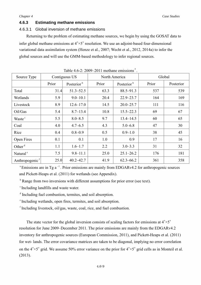
Chapter 4 Case Studies
4.6-9
4.6.3 Estimating methane emissions 4.6.3.1 Global inversion of methane emissions
Returning to the problem of estimating methane sources, we begin by using the GOSAT data to
infer global methane emissions at 4◦×5◦ resolution. We use an adjoint-based four-dimensional variational data assimilation system (Henze et al., 2007; Wecht et al., 2012, 2014a) to infer the
global sources and will use the GMM-based methodology to infer regional sources.
Table 4.6-2: 2009–2011 methane emissions a . Source Type Contiguous US North America Global
Prior Posterior b Prior Posterior b Prior Posterior
Total 31.4 51.3–52.5 63.3 88.5–91.3 537 539
Wetlands 5.9 9.0–10.1 20.4 22.9–23.7 164 169
Livestock 8.9 12.6–17.0 14.5 20.0–25.7 111 116
Oil/Gas 5.4 8.7–13.4 10.8 15.5–22.3 69 67
Waste c 5.5 8.0–8.5 9.7 13.4–14.5 60 65
Coal 4.0 4.7–6.5 4.3 5.0–6.8 47 30
Rice 0.4 0.8–0.9 0.5 0.9–1.0 38 45
Open Fires 0.1 0.1 1.0 0.9 17 16
Other d 1.1 1.6–1.7 2.2 3.0–3.3 31 32
Natural e 7.5 9.8–11.1 25.0 25.1–26.2 176 181
Anthropogenic f 25.0 40.2–42.7 41.9 62.3–66.2 361 358 a Emissions are in Tg a 1− . Prior emissions are mainly from EDGARv4.2 for anthropogenic sources and Pickett-Heaps et al. (2011) for wetlands (see Appendix). b Range from two inversions with different assumptions for prior error (see text). c Including landfills and waste water. d Including fuel combustion, termites, and soil absorption. e Including wetlands, open fires, termites, and soil absorption. f Including livestock, oil/gas, waste, coal, rice, and fuel combustion.
The state vector for the global inversion consists of scaling factors for emissions at 4◦×5◦ resolution for June 2009–December 2011. The prior emissions are mainly from the EDGARv4.2
inventory for anthropogenic sources (European Commission, 2011), and Pickett-Heaps et al. (2011)
for wet- lands. The error covariance matrices are taken to be diagonal, implying no error correlation
on the 4◦×5◦ grid. We assume 50% error variance on the prior for 4◦×5◦ grid cells as in Monteil et al. (2013).

Chapter 4 Case Studies
4.6-10
Observational error variances are estimated following Heald et al. (2004) by using residual
standard deviations of the differences between observations and the GEOS-Chem simulation with
prior emissions. As shown by Heald et al. (2004), this residual error provides an estimate of the
total observational error needed for the inversion, summing the contributions from instrument
retrieval, representation, and model transport errors. We find that the resulting observational error
variances are lower than the local retrieval error variances reported by Parker et al. (2011) for 58%
of the observations, and in those cases we use the latter instead. The implication is that the Parker et
al. (2011) error estimates may be too high but provide a conservative estimate of the observational
error.
The GEOS-Chem forward model and its adjoint are as described by Wecht et al. (2014a). We
optimize methane emissions from 1 June 2009 to 1 January 2012. The forward model is initialized
on 1 January 2009 with concentrations from Wecht et al. (2014a). The 5-month spin-up allows for
the establishment of gradients driven by synoptic motions and effectively removes the influence of
the initial conditions.

Chapter 4 Case Studies
4.6-11
Fig. 4.6-2. Optimization of methane emissions for 2009–2011 at 4◦×5◦ horizontal resolution using GOSAT observations. The panels show prior emissions, posterior emissions, and the ratio between
the two. (from: Turner et al., 2015; their Fig. 3).
Figure 4.6-2 shows the prior and posterior 2009–2011 emissions. The total posterior methane emission is 539 Tg a 1− , unchanged from the prior (537 Tg a 1− ). This source is within the 548 21
22+−
Tg a 1− range of current estimates reported by Kirschke et al. (2013) and IPCC (2013). However, we find large regional differences compared to the prior. Emissions from China are revised
downward by 50% from 29.2 to 14.7 Tg a 1− , consistent with Bergamaschi et al. (2013), who find that EDGARv4.2 Chinese coal emissions are too large. This overestimate in Chinese methane
emissions is also seen by Bruhwiler et al. (2014), who assimilated the 2000–2010 NOAA surface
observations into CarbonTracker using an ensemble Kalman filter. Emissions in India are also too
high, while emissions in Southeast Asia are too low. Emissions from wetlands in central Africa are

Chapter 4 Case Studies
4.6-12
too high. Emissions in northern South America are too low. Corrections in North America are
discussed in the next section.
We inferred the contributions from different source types to our posterior emissions by
assuming that the prior inventory correctly partitions the methane by source type in each 4◦×5◦ grid cell. This does not assume that the global distribution of source types is correct in the prior,
only that the local identification of dominant sources is. We find only modest changes to the global
partitioning by source types, with the exception of coal and rice, partly reflecting regional offsets.
For example, wetland emissions increase globally by only 5 Tg a 1− but decrease by 24 Tg a 1− in
the African wetlands, while increasing by 10 Tg a 1− in northern South America.
4.6.3.2 North American inversion of methane emissions We then optimize methane emissions over North America by using the nested GEOS-Chem
simulation at 1/2◦×2/3◦ horizontal resolution (∼50 km × 50 km) over North America.
Time-dependent boundary conditions for this nested simulation are from the global model at 4◦×5◦ horizontal resolution using the posterior emissions derived above. We only solve for the spatial
distribution of emissions, assuming that the prior temporal distribution is correct.
Fig. 4.6-3. Methane emissions in North America in 2009–2011. The left panels show the prior and
posterior emissions and the bottom right panel shows the scaling factors. The top right panel shows
the diagonal elements of the averaging kernel matrix for the methane emission inversion. The
degrees of freedom for signal (DOFS) is the trace of the averaging kernel matrix. (from: Turner et
al., 2015; their Fig. 4).

Chapter 4 Case Studies
4.6-13
As discussed in Section 4.6.2.3, the dimension of the emissions state vector for the nested
North American inversion is optimally reduced from the native 1/2◦×2/3◦ resolution (n = 7366) in order to (1) improve the observational constraints on individual state vector elements and (2) enable
an analytical inversion with full error characterization. This is done by aggregating similar state
vector elements with a Gaussian mixture model (Bishop, 2007). We find that an optimal reduction
with negligibly small aggregation error can be achieved using 369 radial basis functions (RBFs)
with Gaussian kernels. The RBFs are constructed from estimation of the factors driving error
correlations between the native-resolution state vector elements including spatial proximity,
correction from one iteration of an adjoint-based inversion at 1/2◦×2/3◦ resolution, and prior source type distributions. Including the correction from the adjoint-based inversion allows us to account
for sources not included in the prior. Each 1/2◦×2/3◦ native-resolution grid square is projected onto an aggregated state vector using the RBFs. This preserves native resolution where needed (in
particular for large point sources) and aggregates large regions where emissions are uniformly
small.
Our optimal estimate of North American emissions was obtained by analytical solution to Eq.
(5) using the methodology described in Section 4.6.2.1. This analytical approach provides the
posterior covariance matrix S and averaging kernel matrix A as part of the solution and thus fully characterizes the errors and information content of the inversion results.
The observational error covariance matrix is assumed diagonal with terms specified as the
larger of the residual error variance and the retrieval error variance, same as for the global inversion.
The prior error covariance matrix is assumed diagonal because the radial basis functions are
designed to capture spatial correlations in the emissions. We assume 100% error on emissions at the
native 1/2◦×2/3◦ resolution. For RBFs encompassing larger spatial regions, we assume that the error is reduced following the central limit theorem:
,=,
a},{,a
jij
iiw
sS∑
(18)
where },{,a iiS is the i th diagonal of aS , as is the prior uncertainty at the native resolution
(100%), and the summation is for the weights of the i th RBF over all 1/2◦×2/3◦ grid squares (index j ). This error reduction assumes that the errors on the native-resolution grid cells are independent
and identically distributed, which may be overly optimistic. We examined the sensitivity to this
assumption by conducting an alternate inversion with a relative error of 30% for all state vector
elements, similar to the approach taken by Wecht et al. (2014a) using a hierarchial clustering
method for the state vector.
Figure 4.6-3 shows the prior and posterior 2009–2011 emissions. Total posterior emissions in
North America (Table 4.6-2) are 44% higher than the prior, with large increases in the southern–

Chapter 4 Case Studies
4.6-14
central US and weak decreases for the Canadian wetlands. Contiguous US emissions are 52 Tg a 1− , 70% higher than the prior. The broad correction patterns are consistent with the coarse global
results in Fig. 4.6-2 that used a completely different inversion method. Our sensitivity inversion
assuming 30% prior error on all state vector elements yields the same North American and
contiguous US totals to within 3%.
We evaluated the posterior emissions in a GEOS-Chem simulation over North America by
comparison to the independent observations from the NOAA network. We find great improvement
in the ability of the model to reproduce these observations, as illustrated by the scatterplots of Fig.
4.6-4. The reduced-major-axis (RMA) regression slopes improve from 0.72 to 1.03 for the
NOAA/ESRL tall tower network, from 0.75 to 0.94 for the NOAA/ESRL aircraft profiles, and from
0.67 to 1.01 for the NOAA surface flasks.

Chapter 4 Case Studies
4.6-15
Fig. 4.6-4. Evaluation of the GOSAT inversion of methane emissions for North America with
independent data sets. The scatterplots show comparisons of GEOS-Chem (1/2◦×2/3◦ resolution) methane concentrations with observations from the NOAA/ESRL tall tower network (red),
NOAA/ESRL aircraft program (blue), and the NOAA/ESRL surface flask network (orange), using
prior emissions (top) and posterior emissions (bottom). The 1 : 1 lines (dashed) and
reduced-major-axis (RMA, solid) linear regressions are also shown. (from: Turner et al., 2015; their
Fig. 5).
Another independent evaluation of our posterior emissions is the estimate for California.
California’s methane emissions have been extensively studied with aircraft and ground-based
observations over the past few years in order to address statewide greenhouse gas regulation targets
(Zhao et al., 2009; Wunch et al., 2009; Hsu et al., 2010; Peischl et al., 2012; Wennberg et al., 2012;

Chapter 4 Case Studies
4.6-16
Jeong et al., 2012, 2013; Peischl et al., 2013; Santoni et al., 2014; Wecht et al., 2014b). Figure 4.6-5
shows that our posterior emissions are 20% higher than the EDGARv4.2 prior inventory for the
state of California and 50% lower for the Southern California Air Basin (SoCAB). Other studies
constrained with dense aircraft and ground-based observations are consistent with ours. Wecht et al.
(2014b) previously found that GOSAT observations were not sufficiently dense to constrain
methane emissions in California. However, they only used a 2-month record and tried to constrain
emissions at 1/2◦×2/3◦ resolution, incurring large smoothing error. By using a longer time record and an optimally defined state vector, we achieve much better success.
Fig. 4.6-5. Methane emissions for the state of California (top) and for the Southern California Air
Basin (SoCAB; bottom). Our posterior emissions (this work) are compared to prior emissions
(EDGARv4.2) and to previous inverse estimates constrained by surface and aircraft observations.
SoCAB is defined following Wennberg et al. (2012) as the domain 33.5–34.5◦ N, 117–119◦ W. (from: Turner et al., 2015; their Fig. 6).
Figure 4.6-3 (top right panel) shows the averaging kernel sensitivities for the North American
methane emission inversion, defined as the diagonals of the averaging kernel matrix. The inversion
has 39 degrees of freedom for signal (DOFs), meaning that we can exactly constrain 39 pieces of
information in the distribution of methane emissions. This information is spread over the continent
and mixed with prior constraints as described by the averaging kernel matrix. We can use the
averaging kernel sensitivities in Fig. 4.6-3 to determine which regions are most responsive to the
inversion. These include California, the Canadian wetlands, and the southeastern and central US.

Chapter 4 Case Studies
4.6-17
Large isolated point sources such as the US Four Corners (a large source of coalbed methane at the
corner of Arizona, New Mexico, Colorado, and Utah) are also strongly sensitive to the inversion.
We see from Fig. 4.6-3 that the prior underestimate of North American methane emissions is
largely due to the central US, the Canadian Oil Sands, central Mexico, California, and Florida.
Various large point sources such as the US Four Corners also contribute. We also find regions where
the prior is too high, including the Hudson Bay Lowlands, SoCAB, and parts of Appalachia. This
suggests that oil/gas and livestock emissions are higher than given in EDGARv4.2, while coal
emissions are lower. The overestimate in SoCAB is likely because EDGARv4.2 uses urban and
rural population as a spatial proxy for landfills and waste water (Wunch et al., 2009). The
underestimate in Florida is most likely due to wetland sources.
As with the global inversion, we infer the contributions from different methane source types by
assuming that the prior inventory correctly attributes the source types in a given 1/2◦×2/3◦ grid cell. Again, this does not assume that the prior distribution is correct, only that the identification of
locally dominant sources is correct. Results are shown in Fig. 4.6-6. We see that the increase
relative to the prior is mainly driven by anthropogenic sources. This can be compared to the US
EPA anthropogenic inventory (EPA, 2014), which is based on more detailed bottom-up information
than EDGARv4.2 but is only available as a national total. We find an anthropogenic source for the
contiguous US of 40.2–42.7 Tg a 1− , as compared to 27.0 Tg a 1− in the US EPA inventory. The largest differences are for the oil/gas and livestock sectors. Depending on the assumptions made
regarding the prior error, oil/gas emissions from our inversion are 13–74% higher than the EPA
estimate and contribute 17–26% of contiguous US methane emissions. Livestock emissions are 36–
85% higher than the EPA estimate and contribute 24–33% of contiguous US methane emissions.
Waste and coal emissions are also higher in our posterior estimate than in the EPA inventory.

Chapter 4 Case Studies
4.6-18
Fig. 4.6-6. Methane emissions in the contiguous US. The left panel shows our best estimates of total
and anthropogenic emissions (this work) compared to the prior (EDGARv4.2 for anthropogenic
sources, Pickett-Heaps et al. (2011) for wetlands) and the previous inverse studies of Wecht et al.
(2014a) and Miller et al. (2013). The right panel partitions US anthropogenic emissions by source
types and compares our results (this work) to EDGARv4.2 and to the 2012 EPA inventory (EPA,
2014). Error bars on sectoral emissions for our results are defined by the sensitivity inversion with
30% prior uncertainty for all state vector elements. (from: Turner et al., 2015; their Fig. 7).
4.6.4 Conclusions The sources and sinks of atmospheric methane have proved difficult to constrain (Turner et al.,
2017). Here we presented results from a case study examining global and regional methane
emissions sources. 31 months of observations from GOSAT were used to quantify the methane
sources and were found to be in good agreement with regional estimates obtained from focused
field campaigns. The observations were used in both an adjoint-based and analytical inversion
methodology. The analytical inversion used a reduced-dimension state vector with the state vector
defined by radial basis functions using a Gaussian mixture model. The case study presented here
demonstrates the potential for further monitoring of methane emissions using satellite observations.

Chapter 4 Case Studies
4.7-1
4.7 Joint analysis of CO2 and CH4 inversion fluxes to refine anthropogenic CO2 emissions: A case study of East Asia
Tazu Saeki1 and Prabir K. Patra2
1) National Institute for Environmental Studies (NIES), Japan
2) Japan Agency for Marine-Earth Science and Technology (JAMSTEC), Japan
4.7.1 Introduction
An atmospheric inverse modeling, so called a top-down approach, is an effective way to
estimate global and regional greenhouse gas (GHG) emissions by an atmospheric transport model
and precise measurements of GHG concentrations. The inverse modeling assumes anthropogenic
emissions due to fossil fuel consumption and cement production (FFC) are a known quantity,
because the emissions are calculated from better known industrial indicators, e.g. the gross
domestic product (GDP), import/mining of energy resources, and energy intensity (energy
consumed per unit of GDP). Thus, any bias (uncertainty is assumed 0 in inverse models) in the FFC
emissions would introduce systematic bias in estimation of the terrestrial (residual) fluxes by
inverse modelling.
Recent bottom-up studies have pointed out that the maximum uncertainty in FFC CO2
emissions is clearly found for China (Guan et al. 2012; Liu et al. 2015; Korsbakken et al. 2016). A
top-down model assessment from seven inverse models found that an annual CO2 sink in East Asia
(China, Japan, Korea and Mongolia) increased between 1996–2001 and 2008–2012 by 0.56 PgC on
an average (Thompson et al., 2016). The effort to validate the inverted CO2 fluxes using
independent aircraft CO2 observations did not provide conclusive results as the modeled
concentrations fairly matched the observed vertical gradients between the surface and middle
troposphere as well as the concentrations near the surface layer for a large range (~1 PgC/yr) of
residual CO2 sinks over East Asia alone.
On the other hand, we found the inversion results of CH4 emissions could be successfully
validated using independent aircraft observations over Japan, which suggested an overestimation of
East Asian CH4 emission increase by bottom-up inventories (Patra et al., 2016; Section 4.8 in this
issue). Here we introduce a new approach to use the CH4 inversion results to refine the increase rate
of bottom-up FFC CO2 emissions for East Asia, and show that no systematic increase in land
CO2 uptake over East Asia may be required (as in Saeki and Patra, 2017). The current study used
only surface data for GHG concentrations in inversion analysis, but the results have equal
implications for the use of satellite measurements in an inverse modelling system.
4.7.2 Data We use CO2 observations from 66 sites from GLOBALVIEW-CO2 (2013) data products for

Chapter 4 Case Studies
4.7-2
CO2 inversion analysis to derive CO2 fluxes as described in 4.7.3.2. The GLOBALVIEW dataset
consists of interpolated and smoothed data created from weekly or biweekly flask measurements at
each site. The data uncertainties are assigned to monthly-mean CO2 to account for the ability of
transport models to simulate atmospheric data and the observational accuracy. 4.7.3 Method 4.7.3.1 Outline
First, we conduct CO2 inversions with 3-sets of a priori FFC emissions. We then derive a
scaling factor from CH4 inversion results to correct an increase rate of FFC CO2 emissions. The
CH4 inversion has been validated by independent atmospheric measurements. Because CO2 and
CH4 emissions have strong correlations for some of the emission categories, we took liberty to
apply the CH4-derived scaling factor to refine the a priori FFC CO2 emissions. The CH4-based FFC
emission corrections to inverted CO2 fluxes are applied a posteriori.
4.7.3.2 CO2 inversion CO2 inversions are performed for 2001–2012 to optimize fluxes from 84 regions of the globe
using the JAMSTEC’s atmospheric chemistry-transport model (ACTM) and CO2 observations from
66 sites taken from GLOBALVIEW-CO2 (2013) data products (Saeki and Patra, 2017; Thompson
et al. 2016). We have used three a priori FFC CO2 emission maps from (1) CDIAC: emissions of
top-20 countries from CDIAC (Boden et al. 2016) distributed using EDGAR4 emission maps
(Olivier et al. 2014; 2010 emission maps repeated for the latter years), (2) CARBONES: a project
of the European Union (I. van der Laan-Luijkx, personal communication, 2015; as in Thompson et
al. 2016), and (3) the IEA (International Energy Agency) emissions for South Asia, East Asia,
Southeast Asia and rest of the world distributed using CARBONES emission maps (as in Thompson
et al. 2016; referred to as IEA) (Fig. 4.7-1).

Chapter 4 Case Studies
4.7-3
Figure 4.7-1. FFC CO2 emission map of the CDIAC inventory in 2011 (a), and the differences
between CDIAC emissions for 2011 and 2002 (b), GEOCARBON and CDIAC emissions in 2011
(c), and IEA and CDIAC emissions in 2011 (d).
4.7.3.3 FFC CO2 emission scaling factor from CH4 inversion
CH4 inversions are performed for 53-land regions only, using ACTM forward simulations and
atmospheric data from 39 sites (Patra et al. 2016; Section 4.8. in this issue;). The CH4 inversions
suggested that increase rate of estimated CH4 emissions are 39% (9 Tg) lower than that of a
EDGAR42FT inventory during 2002-2012 (Fig. 4.7-2a). The EDGAR42FT inventory, used as a
priori, suggested an increase of 23 Tg-CH4 emissions from East Asia, which is contributed entirely
by the anthropogenic emission increase rate in China. The validation using independent aircraft
measurement over Sendai by Tohoku University (Umezawa et al. 2014) showed clearly that forward
simulations with the a priori fluxes overestimated the observed CH4 increase but that with the
inverted flux showed good agreement for the net concentration increase during 2002-2012 (see
Section 4.8. for details). We derive a scaling factor of 0.59 (=1.53/2.61, a ratio of slopes of the
linear fits for a posteriori and a priori emissions in Fig. 4.7-2a) to correct an increase rate of a priori
CH4 emissions in East Asia during 2002-2012. The slope of the fitted line to a posteriori CH4
emissions agrees well with a recent inventory emission estimate by Peng et al. (2016). They find
smaller number of deep mining fields in China, which have high CH4 emission factors, compared
that previously assumed.

Chapter 4 Case Studies
4.7-4
Figure 4.7-2. (a) Comparisons of CH4 inversion results (black: a priori; blue: a posteriori) for the
East Asia (EA) region with the EDGAR estimated anthropogenic emissions for China. The linear
fits to the annual mean values are shown as lines, with slopes being marked along the fitted lines.
Recent inventory based CH4 emissions are plotted for a comparison (magenta line; source: Peng et
al., 2016). (b) The linear relationship of anthropogenic CO2 and CH4 emissions for China over the
period of 1970-2012 is evident in the emission inventories, e.g., EDGAR42FT. The inter-decadal
values are marked by text and red circles.
4.7.3.4 Refinement of inverted CO2 fluxes by revised FFC CO2 emissions Since the anthropogenic emissions of both CO2 and CH4 increase linearly in the emission
inventory, we apply a scaling factor of 0.59 derived from the validated CH4 inversion results, to
FFC CO2 emission “increase rate” for the period 2003–2014, relative to the emissions for 2002
from CDIAC inventory. The application of this CH4-inversion-derived scaling factor to the CO2 emission increase rate assumes constant CH4/CO2 emission ratio over the periods of our analyses
and is deemed valid as per the linearity maintained in anthropogenic emission inventories of CO2 and CH4 over the period of 1970–2012 (EDGAR4; Fig. 4.7-2b). The increase in emissions of both
CO2 and CH4 in East Asia is linked to the Chinese coal industry (Fig. 4.7-3); CH4 is emitted during
the coal mining, while emissions of CO2 occur during the consumption of coal primarily in power
plants and industrial combustions (EDGAR42FT2010). About 75% of FFC CO2 emissions and up
to 40% of anthropogenic CH4 emissions are caused due to the coal/oil industry (mining and
burning), which have produced 82% and 72% of the increase in their emissions, respectively, in the
period 2002–2010 (EDGAR42FT).
The inverse model land (residual) fluxes are corrected for the FFC CO2 emission bias
(following Peylin et al. 2013; Thompson et al. 2016). Note that the method is a good approximation
when biases in assumed FFC CO2 emission only in influence land CO2 flux of the same region, but
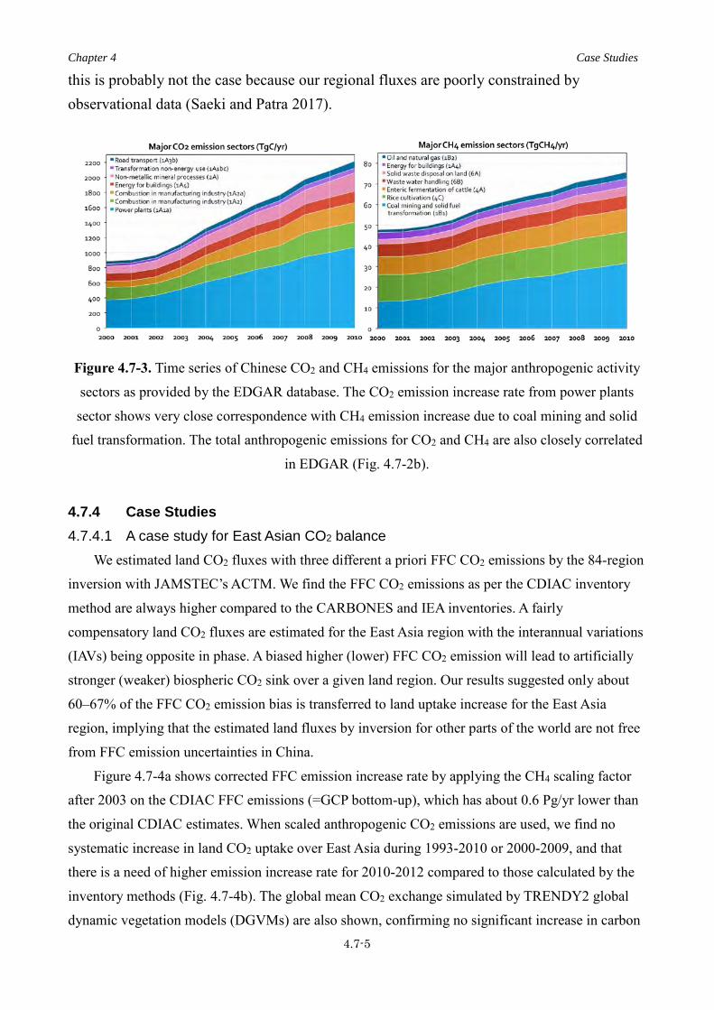
Chapter 4 Case Studies
4.7-5
this is probably not the case because our regional fluxes are poorly constrained by observational data (Saeki and Patra 2017).
Figure 4.7-3. Time series of Chinese CO2 and CH4 emissions for the major anthropogenic activity
sectors as provided by the EDGAR database. The CO2 emission increase rate from power plants
sector shows very close correspondence with CH4 emission increase due to coal mining and solid
fuel transformation. The total anthropogenic emissions for CO2 and CH4 are also closely correlated
in EDGAR (Fig. 4.7-2b).
4.7.4 Case Studies 4.7.4.1 A case study for East Asian CO2 balance
We estimated land CO2 fluxes with three different a priori FFC CO2 emissions by the 84-region
inversion with JAMSTEC’s ACTM. We find the FFC CO2 emissions as per the CDIAC inventory
method are always higher compared to the CARBONES and IEA inventories. A fairly
compensatory land CO2 fluxes are estimated for the East Asia region with the interannual variations
(IAVs) being opposite in phase. A biased higher (lower) FFC CO2 emission will lead to artificially
stronger (weaker) biospheric CO2 sink over a given land region. Our results suggested only about
60–67% of the FFC CO2 emission bias is transferred to land uptake increase for the East Asia
region, implying that the estimated land fluxes by inversion for other parts of the world are not free
from FFC emission uncertainties in China.
Figure 4.7-4a shows corrected FFC emission increase rate by applying the CH4 scaling factor
after 2003 on the CDIAC FFC emissions (=GCP bottom-up), which has about 0.6 Pg/yr lower than
the original CDIAC estimates. When scaled anthropogenic CO2 emissions are used, we find no
systematic increase in land CO2 uptake over East Asia during 1993-2010 or 2000-2009, and that
there is a need of higher emission increase rate for 2010-2012 compared to those calculated by the
inventory methods (Fig. 4.7-4b). The global mean CO2 exchange simulated by TRENDY2 global
dynamic vegetation models (DGVMs) are also shown, confirming no significant increase in carbon
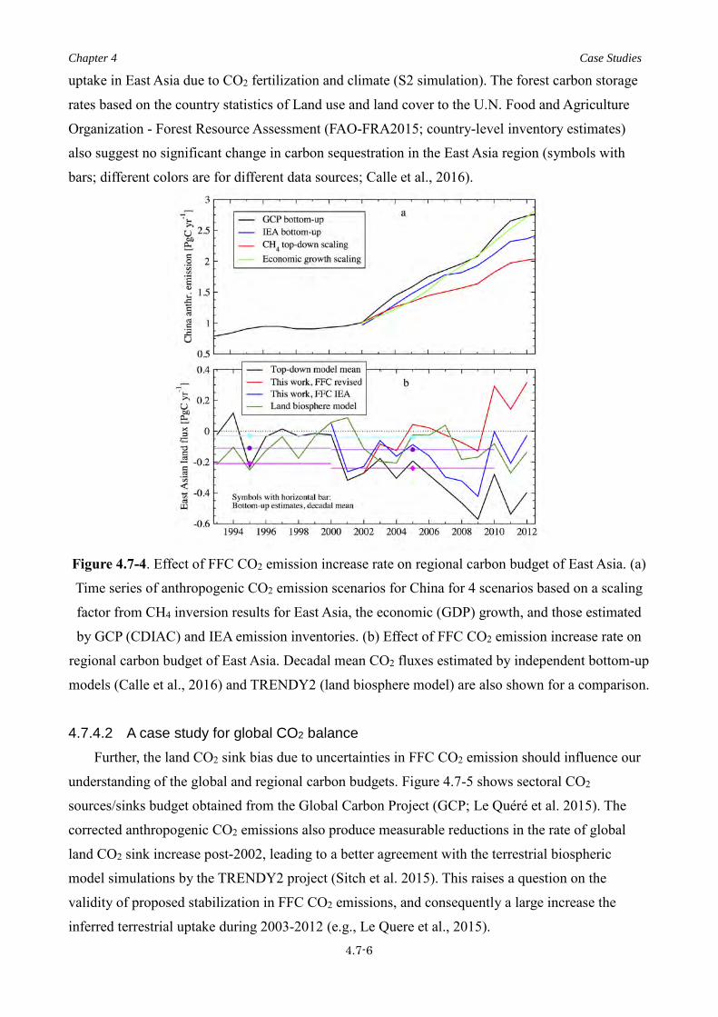
Chapter 4 Case Studies
4.7-6
uptake in East Asia due to CO2 fertilization and climate (S2 simulation). The forest carbon storage
rates based on the country statistics of Land use and land cover to the U.N. Food and Agriculture
Organization - Forest Resource Assessment (FAO-FRA2015; country-level inventory estimates)
also suggest no significant change in carbon sequestration in the East Asia region (symbols with
bars; different colors are for different data sources; Calle et al., 2016).
Figure 4.7-4. Effect of FFC CO2 emission increase rate on regional carbon budget of East Asia. (a)
Time series of anthropogenic CO2 emission scenarios for China for 4 scenarios based on a scaling
factor from CH4 inversion results for East Asia, the economic (GDP) growth, and those estimated
by GCP (CDIAC) and IEA emission inventories. (b) Effect of FFC CO2 emission increase rate on
regional carbon budget of East Asia. Decadal mean CO2 fluxes estimated by independent bottom-up
models (Calle et al., 2016) and TRENDY2 (land biosphere model) are also shown for a comparison.
4.7.4.2 A case study for global CO2 balance
Further, the land CO2 sink bias due to uncertainties in FFC CO2 emission should influence our
understanding of the global and regional carbon budgets. Figure 4.7-5 shows sectoral CO2
sources/sinks budget obtained from the Global Carbon Project (GCP; Le Quéré et al. 2015). The
corrected anthropogenic CO2 emissions also produce measurable reductions in the rate of global
land CO2 sink increase post-2002, leading to a better agreement with the terrestrial biospheric
model simulations by the TRENDY2 project (Sitch et al. 2015). This raises a question on the
validity of proposed stabilization in FFC CO2 emissions, and consequently a large increase the
inferred terrestrial uptake during 2003-2012 (e.g., Le Quere et al., 2015).

Chapter 4 Case Studies
4.7-7
Figure 4.7-5. Time series of CO2 fluxes as estimated by the Global Carbon Project for fossil fuel
and cement (FFC), land-use change (LUC), atmospheric burden increase (ABI), oceanic exchange
(OCN), residual land biosphere (LND = FFC + LUC – ABI − OCN), ensemble mean land fluxes simulated by the global dynamic vegetation models (DGVMs from TRENDY project) during the
period 1999–2014 (top). FFC corrected by CH4 inversion scaling (corFFC) are also shown.
Corrected land fluxes (corLND) is based on residuals calculated using corFFC emissions. Relative
values to the year 1999 are also shown in the lower panel for better clarity on the improved
agreement of corLND fluxes with those simulated by the state-of-the-art DGVMs (bottom).

Chapter 4 Case Studies
4.8-1
4.8 Inversion modeling of global CH4 emissions: results for sub-continental regions of Asia and outlook for satellite data utilization
Prabir K. Patra1, Tazu Saeki2, Shuji Aoki3, Shinji Morimoto3, Takakiyo Nakazawa3, Edward J.
Dlugokencky4, Andre Butz5, and Ronald G. Prinn6
1) Japan Agency for Marine-Earth Science and Technology (JAMSTEC), Yokohama, Japan
2) National Institute for Environmental Studies (NIES), Tsukuba, Japan
3) Graduate School of Science, Tohoku University, Sendai, Japan
4) ESRL, National Oceanic and Atmospheric Administration (NOAA), Boulder, USA
5) Institute of Atmospheric Physics, German Aerospace Center (DLR), Munich, Germany
6) Massachusetts Institute of Technology, Cambridge, USA
4.8.1 Introduction
Methane (CH4) is an important greenhouse gas, second only to carbon dioxide (CO2) for the net
increase in radiative forcing of the Earth’s atmosphere since the preindustrial time (circa. 1750).
The radiative forcing due to naturally occurring water vapour has not changed apparently in the era
of direct measurement [IPCC, 2013]. Methane also participate strongly in the chemistry of
tropospheric air pollution and in modulating stratospheric water vapour budget. Sources and sinks
budgeting of CH4 is thus seen as more challenging compare to CO2, because the latter has the
sources and sinks located on the Earth’s surface and no chemical production/loss is considered in
modelling atmospheric-CO2 [Heimann and Keeling, 1989], while about 90% of CH4 is lost by
reacting with hydroxyl radical (OH) in troposphere. The third most important GHG, nitrous oxide
(N2O) is emitted from the Earth’s surface and has no known loss processes within the troposphere
[Ishijima et al., 2010]; thus no direct link between the photo-chemical loss of N2O and surface
emissions. In contrast to CO2 and N2O, for deriving atmospheric observational constraint on
emission of CH4 on the Earth’s surface requires full knowledge of its chemical loss in the
troposphere. Thus, the distribution and trends in OH should be independently verified for
quantification of chemical sink of CH4, particularly in the troposphere, before performing inverse
modelling of atmospheric-CH4 for estimating surface emissions [Patra et al., 2014].
Inverse modeling, the so called a top-down approach, is commonly employed for estimation of
global and regional greenhouse gases (GHGs) emission by using an atmospheric
chemistry-transport model (CTM) and measurements of GHG concentrations. The accuracy of CH4
sources and sinks modelling depends on the uncertainties in representation of model transport, OH
concentration and size of observational network. For a very long time, small number of in situ
measurements from about 100 sites were the source of atmospheric data for inverse modelling of
CH4 emissions (Patra et al., 2016 and references therein). Only recently, dedicated satellites sensors
are launched for GHGs measurements, e.g., the Greenhouse gases Observation SATellite (GOSAT)

Chapter 4 Case Studies
4.8-2
by JAXA (Kuze et al., 2009). However, the both downward-looking satellites or upward-looking
Fourier-Transform Spectrometers (FTS) measure the total columnar in the atmosphere, which
significantly weakens the link between the variabilities in atmospheric measurements and surface
emissions, compared to the is situ measurements. Thus, a much greater dependence on CTM
simulation is envisaged for inferring surface sources from total column measurement.
4.8.2 Data and Method 4.8.2.1 Atmospheric chemistry-transport model (ACTM)
Methane in atmosphere is simulated using the Center for Climate System Research/National
Institute for Environmental Studies/Frontier Research Center for Global Change
(CCSR/NIES/FRCGC) atmospheric general circulation model (AGCM)-based CTM (i.e.,
JAMSTEC’s ACTM; Patra et al., 2009). The following continuity equation is solved for time (t)
evolution of CH4 at different latitude (y), longitude (x) and altitude (z) in the earth’s atmosphere.
(Eq. 1)
where, CH4 is methane mole fraction in the atmosphere, S is emissions/sinks of CH4 at the surface,
taken from bottom-up emission inventories and terrestrial ecosystem model simulations, L is
temperature (T) dependent loss rates of CH4 due to reaction with OH, O(1D) and Cl, and the last
term: defines transport of CH4 by advection, convection and diffusion. The loss and transport terms
in Equation 1 should be critically evaluated before optimizing bottom-up emissions of CH4. Details
of the ACTM setup are given in Patra et al. (2016).
4.8.2.2 CH4 observations We use atmospheric CH4 measurements in units of dry-air mole fraction (in ppb, parts per
billion) from 37 NOAA/ESRL cooperative global air sampling network sites and 2 Japan
Meteorological Agency sites for estimating monthly-mean emissions by inversion (Fig. 4.8-1). Both
measurement networks reported data on the WMO mole fraction scale (Dlugokencky et al., 2005).
These remote background measurement sites are chosen based on minimal data gap, typically less
than 2 months, for the period of inverse calculation, 2001–2013.
Fig. 4.8-1. Map of 53 land region divisions used
in CH4 inverse modelling by ACTM (Patra et al.,
2016). Locations of 39 measurement sites are
marked by numbers. Observational data are
available from the WMO World Data Center for
Greenhouse Gases (WDCGG).
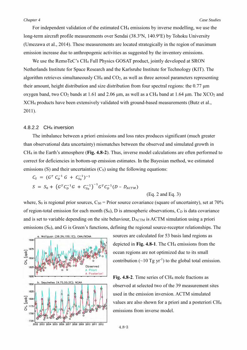
Chapter 4 Case Studies
4.8-3
For independent validation of the estimated CH4 emissions by inverse modelling, we use the
long-term aircraft profile measurements over Sendai (38.3oN, 140.9oE) by Tohoku University
(Umezawa et al., 2014). These measurements are located strategically in the region of maximum
emission increase due to anthropogenic activities as suggested by the inventory emissions.
We use the RemoTeC’s CH4 Full Physics GOSAT product, jointly developed at SRON
Netherlands Institute for Space Research and the Karlsruhe Institute for Technology (KIT). The
algorithm retrieves simultaneously CH4 and CO2, as well as three aerosol parameters representing
their amount, height distribution and size distribution from four spectral regions: the 0.77 μm
oxygen band, two CO2 bands at 1.61 and 2.06 μm, as well as a CH4 band at 1.64 μm. The XCO2 and
XCH4 products have been extensively validated with ground-based measurements (Butz et al.,
2011).
4.8.2.2 CH4 inversion The imbalance between a priori emissions and loss rates produces significant (much greater
than observational data uncertainty) mismatches between the observed and simulated growth in
CH4 in the Earth’s atmosphere (Fig. 4.8-2). Thus, inverse model calculations are often performed to
correct for deficiencies in bottom-up emission estimates. In the Bayesian method, we estimated
emissions (S) and their uncertainties (CS) using the following equations:
(Eq. 2 and Eq. 3) where, S0 is regional prior sources, CS0 = Prior source covariance (square of uncertainty), set at 70%
of region-total emission for each month (S0), D is atmospheric observations, CD is data covariance
and is set to variable depending on the site behaviour, DACTM is ACTM simulation using a priori
emissions (S0), and G is Green’s functions, defining the regional source-receptor relationships. The
sources are calculated for 53 basis land regions as
depicted in Fig. 4.8-1. The CH4 emissions from the
ocean regions are not optimized due to its small
contribution (~10 Tg yr-1) to the global total emission.
Fig. 4.8-2. Time series of CH4 mole fractions as
observed at selected two of the 39 measurement sites
used in the emission inversion. ACTM simulated
values are also shown for a priori and a posteriori CH4
emissions from inverse model.
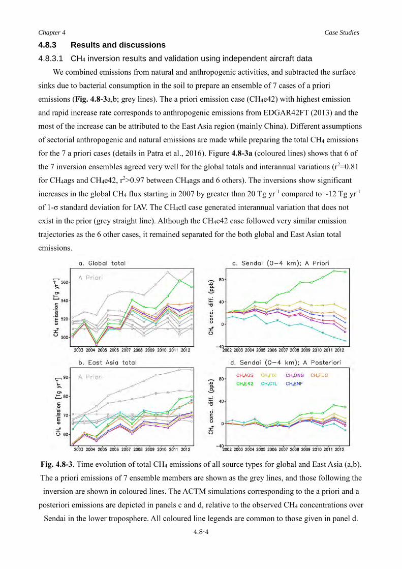
Chapter 4 Case Studies
4.8-4
4.8.3 Results and discussions 4.8.3.1 CH4 inversion results and validation using independent aircraft data
We combined emissions from natural and anthropogenic activities, and subtracted the surface
sinks due to bacterial consumption in the soil to prepare an ensemble of 7 cases of a priori
emissions (Fig. 4.8-3a,b; grey lines). The a priori emission case (CH4e42) with highest emission
and rapid increase rate corresponds to anthropogenic emissions from EDGAR42FT (2013) and the
most of the increase can be attributed to the East Asia region (mainly China). Different assumptions
of sectorial anthropogenic and natural emissions are made while preparing the total CH4 emissions
for the 7 a priori cases (details in Patra et al., 2016). Figure 4.8-3a (coloured lines) shows that 6 of
the 7 inversion ensembles agreed very well for the global totals and interannual variations (r2=0.81
for CH4ags and CH4e42, r2>0.97 between CH4ags and 6 others). The inversions show significant
increases in the global CH4 flux starting in 2007 by greater than 20 Tg yr-1 compared to ~12 Tg yr-1
of 1-σ standard deviation for IAV. The CH4ctl case generated interannual variation that does not
exist in the prior (grey straight line). Although the CH4e42 case followed very similar emission
trajectories as the 6 other cases, it remained separated for the both global and East Asian total
emissions.
Fig. 4.8-3. Time evolution of total CH4 emissions of all source types for global and East Asia (a,b).
The a priori emissions of 7 ensemble members are shown as the grey lines, and those following the
inversion are shown in coloured lines. The ACTM simulations corresponding to the a priori and a
posteriori emissions are depicted in panels c and d, relative to the observed CH4 concentrations over
Sendai in the lower troposphere. All coloured line legends are common to those given in panel d.

Chapter 4 Case Studies
4.8-5
For validating the CH4 emission increase rate, we show model – measurement differences of
CH4 over Sendai, Japan in Fig. 4.8-3c,d. The simulated mole fractions calculated with a posteriori
emissions agree with the measured values within 0.3% (5 ppb) for individual years, except for
CH4e42 case. The vertical gradients are also well simulated for 2002–2012 (not shown) with typical
model-observation differences lower than 20 ppb. These comparisons clearly indicate that the
CH4e42 inversion case still overestimates emissions of CH4 from the East Asia region. Our best
estimated emission increase is 7–8 Tg yr-1 over the periods of 2002–2006 and 2008–2012, by
excluding the CH4e42 case. It should be pointed out here that a posteriori uncertainty (CS) was
about 22 Tg yr-1 for the East Asia region, which does not truly reflect the quality of mean a
posteriori flux by the 6 inversion ensembles. The quality of the mean fluxes is better evaluated
(within 10 Tg yr-1) using independent aircraft measurements. The net increase in CH4 emissions by
inversion for East Asia has large implications for CO2 inversions (Saeki and Patra, 2017).
4.8.3.2 Linking inter-hemispheric CH4 balance with north-south hemispheric OH gradient As mentioned earlier, most of CH4 in atmosphere are lost due to reaction with OH. Because of
its very short lifetime (~1 sec) and very low abundance (~106 molecules cm-3) in the troposphere, an
accurate characterization of OH distributions and strength has remained elusive. Use of methyl
chloroform (CH3CCl3) is found to be ideal for characterizing OH, because emission of this
man-made species is regulated stringently by the Montreal Protocol in 1988 due its strong ozone
depletion potential, and the local lifetimes of CH3CCl3 is 1–3 years in the tropical troposphere,
which is of similar magnitude as the interhemispheric transport time of ~1.3 years. The latter
condition is important for evaluating northern-to-southern (NH/SH) ratio of hemispheric mean OH.
Using the time evolution of CH3CCl3 simulation, the balance between global total emissions and
global mean OH concentrations can be established (Fig. 4.8-4a). We use pre-defined tropospheric
OH concentrations from Spivakovsky et al. (2000) (referred to as ACTM_0.99 as the NH/SH OH
ratio is 0.99) and Sudo et al. (2002) (referred to as ACTM_1.26 as the NH/SH OH ratio is 1.26).
From the observed differences in CH3CCl3 between MHD and CGO from two ACTM simulations
(Fig. 4.8-4b), equal amount OH in both the hemispheres is suggested (Patra et al., 2014).
One of the important implications of correctly estimating the NH/SH OH ratio is for the
budgets of many important short-lived species that affect the Earth’s radiative budget and air
pollution chemistry. Impact of using ACTM_0.99 and ACTM_1.26 OH fields on CH4 emission
estimation is studied using our newly developed inverse modeling system [Patra et al., 2016]. The
inverse estimated CH4 emissions are clearly biased high in the NH mid-high latitude regions and
generally biased low (compensatory for global totals) in the tropical and SH land regions when
ACTM_1.26 is used in forward modelling of CH4, compared to the use of more accurate
representation of OH in ACTM_0.99 (Fig. 4.8-5). The NH total CH4 emission estimated to be 18 Tg

Chapter 4 Case Studies
4.8-6
yr-1 higher for ACTM_1.26 (and 15 Tg yr-1 lower in the SH), compared that for ACTM_0.99.
Fig. 4.8-4. Time series of CH3CCl3 concentrations (a) and inter-sites gradients (b) as observed by
AGAGE network (Prinn et al., 2000) at Mace Head (MHD) and Cape Grim (CGO) and simulated
by ACTM_0.99 and ACTM_1.26 simulations.
Fig. 4.8-5. Differences in inversion
estimated CH4 emissions due to the use of
two different OH distributions in ACTM
simulations. The 12 regions identified as
the x-tick labels are obtained by
aggregating 53 regions of the inverse
model as depicted in Fig. 4.8-1.
4.8.4 Outlook for GOSAT CH4 utility One of the major limitations for inverse modelling of GHG sources/sinks is the lack of
sufficient in situ measurement stations, say covering each of the 53-regions of the inverse model
(Fig. 4.8-1). However, this limitation should be relaxed provided high density and high-quality
measurements of CH4 are made from space. Although progress is being made in understanding the
information content in GOSAT XCH4 retrievals over the Asian regions (Ishizawa et al., 2016;
Chandra et al., 2017), various retrieval biases and uncertainties in forward model simulations still
keep the GOSAT data usage at minimal for CH4 inverse modelling (e.g., Pandey et al., 2016).
An overall agreement is found between the maps of CH4 emissions and GOSAT XCH4
distributions for the high emissions and CH4 over the Indo-Gangetic Plain (IGP) and most parts of
eastern China (Figure 4.8-6a,b,d). The east-west gradients in CH4 over IGP by model simulations
show different feature when simulated by ACTM_0.99, where simulation using CH4ags emission
case show much higher XCH4 over Bangladesh compared to the ACTM simulation using CH4ctl

Chapter 4 Case Studies
4.8-7
case and the retrievals by SRON/KIT. The XCH4 seasonality using CH4ags emission also peaks
earlier compared to the observations due to early peak in emissions (Figure 4.8-6c,g,h). This
suggests the GOSAT XCH4 values contains information for constraining regional CH4 emission
over the South Asia region. It may be noted here that the data density over the South Asia region is
sparse during the summer monsoon season (June-Sept.) due to dense cloud cover. Further analysis
is needed for understanding the causes for large differences found between the GOSAT XCH4 and
both the ACTM simulations over the northern Southeast Asia and southern China. These regions are
largely unconstrained by the in situ measurement sites used the inversion.
Fig. 4.8-6. Maps of CH4 emissions (a,b) and total column XCH4 concentrations (d,e,f) are
compared. Time series of CH4 fluxes and XCH4 time series are shown for seasonal cycle
comparisons (c,g,h). The simulations are conducted by ACTM_0.99 version of the model.

Chapter 4 Case Studies
4.9-1
4.9 Quantifying CO2 Emissions from Individual Power Plants from Space Ray Nassar1, Timothy G. Hill2, Chris A. McLinden1, Debra Wunch3, Dylan B.A. Jones3,
and David Crisp4
1) Environment and Climate Change Canada, Toronto, ON, Canada
2) University of Waterloo, Waterloo, ON, Canada
3) University of Toronto, Toronto, ON, Canada
4) Jet Propulsion Laboratory, California Institute of Technology, Pasadena, CA, USA
4.9.1 Introduction Although the Orbiting Carbon Observatory 2 (OCO-2) was not designed for quantifying
emissions at the scale of an individual power plant, its limited potential to do so was foreseen in
“Verifying Greenhouse Gas Emissions: Methods to Support International Climate Agreements”
[Pacala et al., 2010]. In selected clear-sky cases, where direct OCO-2 overpasses or close flybys of
individual mid- and large-sized coal power plants occur, OCO-2’s narrow swath can image a
segment of the CO2 emission plume, enabling quantification of the emissions with a method
adapted from studies for CarbonSat [Bovensmann et al., 2010]. This is first demonstrated by
quantifying daily CO2 emissions from US power plants by fitting the observed XCO2 enhancements
from OCO-2 to enhancements simulated by a Gaussian plume model, along with a system for
estimating uncertainties. These daily emission estimates and uncertainties are compared with
publicly-available CO2 emission data from the US Environmental Protection Agency (EPA). Next,
the approach is used to derive emissions from a large coal power plant in India that has less detailed
publicly available emission data and higher uncertainties. Although more complex modeling or data
analysis could improve emission estimates, Nassar et al. [2017] demonstrates for the first time, the
ability to quantify emissions from individual power plants with CO2 satellite data. The potential of
some upcoming and proposed CO2 satellites to provide improved capabilities is also discussed.
Overall, the Nassar et al. [2017] results affirm that a future constellation of CO2 imaging satellites,
optimized for point sources, could contribute to the monitoring, reporting and verification (MRV) of
CO2 emissions from individual power plants to support the transparency framework of climate
agreements and the implementation of emission reduction policies.
4.9.2 Data 4.9.2.1 GHG Concentration Data and Other Data
A list of coordinates for mid- to large-sized coal power plants (emitting > 10 MtCO2/yr) is
generated from EPA data (https://ghgdata.epa.gov/ghgp/main.do#/listFacility/) for the US and from
the Carbon Monitoring for Action (CARMA) (www.carma.org) [Wheeler & Ummel, 2008; Ummel,
2012] and the Global Energy Observatory (GEO) databases (www.globalenergyobservatory.org)

Chapter 4 Case Studies
4.9-2
elsewhere. CARMA has global power plant CO2 emission data for 2004, 2009 and ‘Future’, but its
power plant locations can be unreliable, while the GEO database has more accurate location
information (verified by inspection of sites in Google Earth) but little to no CO2 emission data. We
search OCO-2 L2 version 7r XCO2 standard files from Sep 2014 – Dec 2016 inclusive for
overpasses near sites of interest from the databases identified above. Aqua MODIS imagery of
clouds, smoke, and surface properties can be viewed together with OCO-2 data since the Aqua
satellite follows OCO-2 by 6 minutes in the A-Train. For each date and time of an OCO-2 overpass
of a power plant found, ERA-Interim (~0.75°, 60 vertical levels) [Dee et al., 2011] and MERRA2
(0.5°x0.625°, 72 levels) [Molod et al., 2015] meteorological reanalysis files are acquired.
4.9.3 Method 4.9.3.1 Meteorology and Data Visualization
CO2 transport from a power plant depends on the horizontal wind speed at the plume height. A
power plant can have multiple stacks, so we calculate the emission-weighted mean stack height
from available information or assume 250 m. We read the u and v winds for the levels above and
below the mean stack height from the two meteorological data sets and vertically linearly
interpolate to the mean stack height. ERA-Interim winds are reported as instantaneous values at
6-hour intervals, so we also linearly interpolate between the two nearest temporal points. For
MERRA2, which is provided as 3-hour average winds, we use the closest time directly. The
interpolated u and v wind vectors are converted to a scalar wind speed and direction/bearing
(0-360°) with 0° defined as due North. KML files are generated to visualize the
parallelogram-shaped OCO-2 soundings in Google Earth with a customized XCO2 color scale and
wind vector arrows centered on each source. The XCO2 value mapped with the KML file and used
in the emission estimate is a bias corrected value, but uncorrected XCO2 and two variations on the
bias correction are also included in the file. We view the KML files to look for overpasses or flybys
with an enhancement in the approximate wind direction. We reject overpasses where the wind
blows away from the swath, those in regions with complex terrain, or where the swath is broken up
due to cloud or aerosol, since neighbouring observations could be biased, but if nadir observations
are lost over a small body of water, we retain confidence in the remaining observations. KML files
for these case studies are available at ftp://ccrp.tor.ec.gc.ca/pub/RNassar/GRL_Power_Plants/.
4.9.3.2 Plume Model and Fitting For each good overpass or flyby, we take the magnitude of the vector mean of the ERA-Interim
and MERRA2 winds as the wind speed to model the plume. The plume model equations used are
slightly modified from those in Bovensmann et al. [2010]:

Chapter 4 Case Studies
4.9-3
𝑉𝑉(𝑥𝑥, 𝑦𝑦) = 𝐹𝐹√2𝜋𝜋𝜎𝜎𝑦𝑦(𝑥𝑥)𝑢𝑢
𝑒𝑒−12�
𝑦𝑦𝜎𝜎𝑦𝑦(𝑥𝑥)�
2
and 𝜎𝜎𝑦𝑦(𝑥𝑥) = 𝑎𝑎 ∙ � 𝑥𝑥𝑥𝑥𝑜𝑜�0.894
[Eq. 1 and 2]
where V is the CO2 vertical column in (g/m2) at and downwind of the point source. The x-direction
is parallel to the wind direction and the y-direction perpendicular to the wind direction. V depends
on the emission rate F (in g/s), the across wind distance y (in m), wind speed u (in m/s), and the
standard deviation in the y-direction, σy (in m). Here x is specified in m and xo=1000 m is a characteristic length so that the argument of the exponent is dimensionless. a is the atmospheric
stability parameter, which we determine by classifying a source environment by the
Pasquill-Gifford stability, which depends on the surface wind speed, cloud cover and time of day
[Pasquill, 1961]. The surface wind speed and cloud cover are taken from ERA-Interim.
We select a region of the OCO-2 swath (preferably upwind and thus not affected by the source)
as the background and average the XCO2 from these points. The model plume is then defined as the
area from the x-axis (wind vector) down to a threshold of 1% intensity in the positive/negative
y-directions. We then define the observed plume based on the points that correspond to the model
plume, accounting for the light path. We determine where the incoming and reflected solar radiation
would intersect the plume, assuming a 2-dimensional plume at the mean stack height and ignoring
plume rise. Once the observed plume is defined as the points geometrically corresponding to a 1%
cut-off of the model plume, the background XCO2 average in ppm is subtracted from it to get the
observed XCO2 enhancement in ppm. To convert the model enhancements from g/m2 to ppm, we
use the mean conversion factor k, which we calculate from the background values in g/m2 and ppm
given in the data files, where k = VCO2 / XCO2. This is reliable only if there are no large or abrupt
changes in topography for the background. If the wind is nearly parallel to the swath, we truncate
the plume at some distance from the source to avoid very small relative enhancements and plume
modeling over long space/time scales.
With the observed and model plume defined as XCO2 enhancements in ppm, we then calculate
the model versus observation correlation coefficient (R). This process is repeated testing
adjustments to the wind direction to maximize the correlation. We accept a rotation to the wind if it
improves R, passes visual inspection and is consistent with the level of disagreement between the
ERA-Interim and MERRA2 winds. Fitting for the wind direction reduces the impact of errors in the
wind direction from the meteorological fields. Using the optimized wind direction, we determine
the a posteriori emissions by carrying out a weighted linear least squares fit between the model and
observed enhancements calculated per unit emissions. The weights in the least squares fit are the
reciprocal of the XCO2 uncertainty values from the OCO-2 full files. We estimate emissions as
ktCO2/day (1 kt = 106 kg).
Chapter 4 Case Studies
4.9-4
4.9.3.2 Emission Uncertainties Bovensmann et al. [2010] state that since the emission estimate is linearly-dependent on wind
speed, an error in the wind speed contributes linearly to an error in the emission estimate (i.e. a 10%
error in the wind speed contributes a 10% error to the emission estimate). In actuality, the error
dependence is slightly more than linear because the wind speed indirectly affects σy via a. We
calculate the wind uncertainty contribution (εw) to the emission estimate as the percent difference of the two different wind fields from the mean and convert this to an emission rate uncertainty in
ktCO2/day. The background CO2 concentration is a source of uncertainty in this work and in any
work where an enhancement is defined with respect to the background, whether determining the
emissions from a power plant, megacity or volcano. We define the background in 4 different yet
plausible ways, calculating the spread in emission estimates from this small ensemble to get a
standard deviation (εb) in ktCO2/day. If the ensemble gives a large spread, then εb is large and
results in a large overall uncertainty for the emission estimate. If εb is too large, a good background cannot be established and we reject the overpass for quantifying emissions.
The emission uncertainty due to uncertainties in the OCO-2 observations (εe) is also considered using an ensemble. The enhancement relative to the background is calculated multiple times with an
ensemble of 4 bias correction approaches, as described in the supporting information. Our ensemble
approach effectively quantifies the sensitivity of the multi-step emission estimate to biases of the
sizes and patterns that could result by applying the different bias corrections, which provides a good
estimate of the potential uncertainty in the emission estimate arising from the OCO-2 data. Another
source of uncertainty is that due to secondary sources (εs), but as it is only non-zero for one example, it is explained later. The total error is then determined from the wind, background,
enhancement and secondary source terms: 𝜀𝜀 = �𝜀𝜀𝑤𝑤2 + 𝜀𝜀𝑏𝑏2 + 𝜀𝜀𝑒𝑒2 + 𝜀𝜀𝑠𝑠2 [Eq. 3]. Uncertainty related to neglecting plume rise due to thermal lifting in determining the altitude selected for the
wind speed is difficult to quantify and has not been included above, but is discussed in Nassar et al.
[2017] supporting information.
4.9.4 Case Studies 4.9.4.1 A Direct Overpass of a Power Plant in the U.S.
For a direct OCO-2 nadir overpass with the wind nearly aligned with the orbit track, both the
base and center of the plume are imaged, and the background is the portion of the swath upwind
from the source. This alignment is very rare for OCO-2 due to its narrow swath. One occurrence
was a flyover on 2015-12-04 of the Westar Jeffrey Energy Center (Fig. 4.9.1), a mid-sized
sub-bituminous coal-fired power plant in Kansas with three 175-m tall stacks and annual 2015
emissions of 12.5 MtCO2. The observed enhancement is small (~1 ppm) since the emissions were
dispersed quickly by strong winds (~11 m/s). The EPA provides hourly to annual CO2 emissions for

Chapter 4 Case Studies
4.9-5
individual facilities (https://ampd.epa.gov/ampd/) and on this date, reported 26.7 ktCO2/day. A
model fit to the observations gave a daily estimate of 31.2±3.7 kt, with uncertainty contributions
due to wind speed (0.85 kt), the background definition (1.8 kt) and the enhancement (3.1 kt).
Figure 4.9-1. Direct OCO-2 overpass in the U.S. (a) XCO2 from OCO-2 near the Westar Jeffrey
Energy Center shown in Google Earth with ERA-Interim (red) and MERRA2 (blue) wind vectors.
(b) Plume points (red), background points (blue), and the background mean (green line). (c)
Observed XCO2 relative to the background. (R is the correlation coefficient and a is the
atmospheric stability parameter). (d) Gaussian plume model XCO2 plume relative to the
background. (e) Gaussian plume model XCO2 relative to the background as would be viewed by
OCO-2. Solid lines in panels c–e show the model 1% plume density cutoff from the axial value.
4.9.4.2 A Close Flyby of a Power Plant in the U.S.
Figure 4.9-2. Same as Figure 1 for a flyby of the Ghent Generating Station. The dotted lines in
panels c–e show an offset for defining the background with respect to the plume edges.

Chapter 4 Case Studies
4.9-6
In a close flyby, OCO-2’s swath does not pass directly over the source. An example is a flyby
~8 km from the Ghent Generating Station (Fig. 4.9.2), a coal-fired generating station in Kentucky
that emitted 11.0 MtCO2 in 2015. OCO-2 observes a strong enhancement on 2015-08-13 since the
wind speed is very low, yet uncertain (0.50 m/s ERA-Interim, 1.54 m/s MERRA2). Reported CO2
emissions on this date were 29.2 kt and we estimate 29.5±15.6 kt. Uncertainties in wind speed
contribute the majority (15.0 kt) of the large emission uncertainty in this result.
4.9.4.3 Application of the Method to a Large Power Plant in India Our best example of quantifying emissions from a power plant using OCO-2 comes from a
flyover of the Singrauli region of India (Fig. 4.9.3) with multiple large coal plants in close
proximity. Our initial aim was to quantify emissions from the Vindhyachal and Singrauli power
plants, which emitted 32.4 and 14.8 MtCO2/yr respectively (CARMA future values). However, due
to the spatial gradients and the strength of the XCO2 enhancement (~10 ppm) in a 2014-10-23 flyby
of these power plants, we found another major source directly below the enhancement using Google
Earth. The new source detected was the Sasan Ultra Mega Power Plant (UMPP), which was
commissioned between 2013 and 2015. Sasan only appears in CARMA as a future emitter with an
estimate of 33.7 MtCO2/yr, but this estimate assumes a very high emission intensity (1.26
tCO2/MWh).
Figure 4.9-3. Same as Figure 1 for a direct overpass of a large power plant in India with multiple
other power plants nearby. Model simulations here include the primary source (Sasan) plume and
two secondary source (Vindhyachal and Singrauli) plumes superimposed.
Sasan’s Clean Development Mechanism (CDM) application to the UNFCCC (Greenhouse Gas
Reductions Through Super-Critical Technology - Sasan Power Ltd. Clean Development Mechanism

Chapter 4 Case Studies
4.9-7
Project Design Document Form (CDM-PDD), version 3, 2006-07-28) states that at full capacity it
was expected to emit 26.38 MtCO2/yr. It has since received credits for certified emission reductions
since its supercritical coal technology is claimed to emit ~9% less CO2 than standard coal
combustion. Vindhyachal and Singrauli are 14 and 16 km northeast and upwind of Sasan
respectively, so we account for their emissions in the OCO-2 swath (Fig 4.9.3d, e), but two other
large coal power plants, Rihand (20.3 MtCO2/yr) and Anpara (16.8 MtCO2/yr), are farther away and
due to the wind direction, we consider their impact to be negligible. Only 5 of 6 units at Sasan were
commissioned at the time of the flyover, so we assume 5/6 of the total output or a mean daily
emission rate of 60.2 kt. The OCO-2 data yield an estimate of 67.9±10.0 kt with uncertainty
contributions from wind (5.2 kt), the background (0.59 kt), the enhancement (3.2 kt) and an
additional error term for the presence of secondary sources (5.6 kt), determined by perturbing the
CARMA values by ±20%, which gave a perturbation to the estimated emissions of ±5.6 ktCO2/day
(εs in equation 3). We also tested the sensitivity of the result to the along-wind length of plume used ranging from 20-50 km, but it had a smaller impact than any of the error terms included. With this
large XCO2 enhancement, a well-defined background and good consistency in winds, our
uncertainty is 14.7% of the estimated emission value, but would be only 9.1% if not for the
secondary sources.
4.9.4.4 Discussion and Conclusions from Case Studies Gaussian plume models are attractive for their simplicity, but like all models, have limitations,
so we applied the model only to flat regions and to moderate distances and times (up to ~50 km, ~3
h) since our implementation assumes constant emissions and wind speed and direction, assumptions
that degrade over longer distances and times. Table 1 in Nassar et al. [2017] shows emission
estimates for 3 US power plants, 1 in India and 1 in South Africa, including the case studies above.
US emission estimates are within 1%, 4% and 17% of the EPA daily values. Internationally, only
annual values (from another year) are available, so we calculated mean daily values. Typically,
uncertainties related to wind speed were the largest contributor to total uncertainty, which could
potentially be reduced with higher space-time resolution wind fields. The background CO2
concentration was another source of uncertainty, which we dealt with by avoiding overpasses with
ambiguous backgrounds or using an ensemble of background definitions. OCO-2 bias and precision
both contribute to the enhancement uncertainty term, which was usually lower than the uncertainty
due to wind. The low uncertainty contribution from the observations means that the accuracy and
precision of OCO-2 are adequate for quantifying emissions from large and mid-sized coal power
plants and its real limitation is coverage. OCO-2 is a global sampling mission with a narrow swath,
not a mapping mission, so there are wide gaps between successive orbit tracks. Since so much of
the Earth is covered by clouds at any given moment and XCO2 retrievals are very sensitive to cloud
Chapter 4 Case Studies
4.9-8
contamination, ~90% of XCO2 observations from OCO-2 and other CO2 missions are rejected, with
some variation based on observing geometry, field-of-view size and cloud detection methods. As a
result, in ~2 years of OCO-2 data there is rarely more than 1-2 overpasses that are sufficiently
uninterrupted by cloud and have an appropriate wind direction for any given power plant.
To quantify CO2 emissions from individual power plants from space, precise CO2 imaging with
good spatial resolution and coverage is essential. China’s TanSat adds to the coverage currently
obtained from OCO-2 and the upcoming OCO-3 will have an emphasis on targeting cities and power
plants, but these LEO imaging missions will still only enable point source quantification in select
cases. Wider-swath LEO missions would be a benefit; however, estimating annual emissions,
arguably the most policy-relevant time scale for MRV, requires multiple clear-sky revisits in a given
year, which is likely not possible to obtain from a single LEO mission. The number of revisits
required (considering seasonal and diurnal variations) must be established in future work, but with
enough overpasses, annual emission estimates should have lower relative uncertainties than
single-overpass daily values. The Sentinel-7 candidate constellation of 3-4 CO2 monitoring LEO
satellites could potentially provide the required sampling frequency. Imaging from geostationary
orbit (GEO) like NASA’s future GeoCarb mission or other GEO concepts is another approach that
would offer diurnal sampling over land with the flexibility for very frequent observations by targeting
priority locations or cloud-free areas. GEO satellites positioned to observe the Americas,
Europe/Africa and East Asia could provide a system for monitoring low to mid latitude sources,
while highly elliptical orbit (HEO) satellites [Nassar et al., 2014] could view higher latitudes.
Nassar et al. [2017] presents the first detection and quantification of CO2 emissions from
individual facilities using space-based observations, and has yielded daily emission estimates for coal
power plants with reasonable accuracy and precision. The results were obtained with observations
from OCO-2, a mission not designed for this purpose, and suggest that a constellation of multiple
CO2 imaging satellites optimized for point sources could provide data for regular policy-relevant CO2
emission quantification for mid- and large-sized fossil fuel burning power plants across the world.

Appendix-1 References
Appendix 1-1
APPENDIX-1 REFERENCES Aggarwal, C. C. (2015), Data Mining: The Textbook, Springer, New York.
Alexe, M., et al. (2015), Inverse modelling of CH4 emissions for 2010–2011 using different satellite
retrieval products from GOSAT and SCIAMACHY, Atmospheric Chemistry and Physics, 15,
113–133, doi:10.5194/acp-15-113-2015.
Bergamaschi, P., et al. (2009), Inverse modeling of global and regional CH4 emissions using
SCIAMACHY satellite retrievals, J. Geophys. Res., 114, D22301, doi:10.1029/2009JD01228.
Bergamaschi, P., et al. (2013), Atmospheric CH4 in the first decade of the 21st century: Inverse
modeling analysis using SCIAMACHY satellite retrievals and NOAA surface measurements,
Journal of Geophysical Research: Atmospheres, 118, 7350–7369, doi:10.1002/jgrd.50480.
Bergamaschi, P., et al. (2018), Inverse modelling of European CH4 emissions during 2006-2012
using different inverse models and reassessed atmospheric observations, Atmos. Chem. Phys., 18,
901-920, doi: 10.5194/acp-18-901-2018.
Beusse, R., et al. (2014), Improvements needed in EPA efforts to address methane emissions from
natural gas distribution pipelines, 14-P-0324, US EPA Office of Inspector General, available at:
https://www.epa.gov/sites/production/files/2015-09/documents/20140725-14-p-0324_0.pdf (last
access: 28 Sep 2017).
Bishop, C. M. (2007), Pattern Recognition and Machine Learning, Springer, 1 edn.
Bocquet, M. (2009), Toward Optimal Choices of Control Space Representation for Geophysical
Data Assimilation, Monthly Weather Review, 137, 2331–2348, doi:10.1175/2009mwr2789.1.
Bocquet, M., et al. (2011), Bayesian design of control space for optimal assimilation of observa-
tions. Part I: Consistent multiscale formalism, Quarterly Journal of the Royal Meteorological
Society, 137, 1340–1356, doi:10.1002/qj.837.
Boden, T. A., et al. (2016), Global, Regional, and National Fossil-Fuel CO2 Emissions. In: Carbon
Dioxide Information Analysis Center, Oak Ridge National Laboratory, U.S. Department of
Energy, Oak Ridge, Tenn., U.S.A., doi:10.3334/CDIAC/00001_V2016.
Bovensmann, H., et al. (1999), SCIAMACHY - Mission objectives and measurement modes, J.
Atmos. Sci., 56, (2), 127-150.
Bovensmann, H., et al. (2010), A remote sensing technique for global monitoring of power plant
CO2 emissions from space and related applications, Atmos. Meas. Tech. 3, 781–811.
Bréon, F. M., et al. (2015), An attempt at estimating Paris area CO2 emissions from atmospheric
concentration measurements, Atmos. Chem. Phys., 15, 1707-1724,
https://doi.org/10.5194/acp-15-1707-2015.
Brioude, J., et al. (2013), Top-down estimate of surface flux in the Los Angeles Basin using a
mesoscale inverse modeling technique: assessing anthropogenic emissions of CO, NOx and CO2
Appendix-1 References
Appendix 1-2
and their impacts, Atmos. Chem. Phys., 13(7), 3661-3677, doi:10.5194/acp-13-3661-2013.
Broquet, G., et al. (2011), A European summertime CO2 biogenic flux inversion at mesoscale from
continuous in situ mixing ratio measurements, J. Geophys. Res., 116, D23303,
doi:10.1029/2011JD016202.
Bruhwiler, L., et al. (2014), CarbonTracker-CH4: an assimilation system for estimating emissions of
atmospheric methane, Atmospheric Chemistry and Physics, 14, 8269–8293,
doi:10.5194/acp-14-8269-2014.
Bruhwiler, L., et al. (2017), US CH4 emissions from oil and gas production: Have recent large
increases been detected?, J. Geophys. Res., 122(7), 4070-4083, doi:10.1002/2016JD026157.
Buchwitz, M., et al. (2000), A near-infrared optimized DOAS method for the fast global retrieval of
atmospheric CH4, CO, CO2, H2O, and N2O total column amounts from SCIAMACHY Envisat-1
nadir radiances, J. Geophys. Res. 105, 15,231-15,245.
Buchwitz, M., et al. (2015), The Greenhouse Gas Climate Change Initiative (GHG-CCI):
comparison and quality assessment of near-surface-sensitive satellite-derived CO2 and CH4
global data sets, Remote Sensing of Environment, 162, 344-362, doi:10.1016/j.rse.2013.04.024.
Buchwitz, M., et al. (2016), Global satellite observations of column-averaged carbon dioxide and
methane: The GHG-CCI XCO2 and XCH4 CRDP3 data set, Remote Sensing of Environment (in
press), DOI: 10.1016/j.rse.2016.12.027, pp. 20.
Buchwitz, M., et al. (2017), Satellite-derived methane hotspot emission estimates using a fast
data-driven method, Atmos. Chem. Phys., 17(9), 5751-5774, doi:10.5194/acp-17-5751-2017.
Burrows, J., et al. (1995), SCIAMACHY – Scanning Imaging Absorption Spectrometer for
Atmospheric Chartography, Acta Astronaut., 35, 445–451.
Butz, A., et al. (2011), Toward accurate CO2 and CH4 observations from GOSAT, Geophysical
Research Letters, 38, doi:10.1029/2011gl047888, 2011.
Calle, L., et al. (2016), Regional Carbon Fluxes from Land Use and Land Cover Change in Asia,
1980-2009, Env. Res. Lett., 11, 074011, doi:10.1088/1748-9326/11/7/074011.
Caulton, D. R., et al. (2014), Toward a better understanding and quantification of methane
emissions from shale gas development, Proc. Natl. Acad. Sci. U. S. A., 111(17), 6237–6242,
doi:10.1073/pnas.1316546111.
Chandra, N., et al. (2016), What controls the seasonal cycle of columnar methane observed by
GOSAT over different regions in India?, Atmos. Chem. Phys., in review.
Chen, Z., et al. (2007), Correlative Learning: A Basis for Brain and Adaptive Systems, John Wiley
& Sons, New York, 1st edn.
CIESIN/CIAT, CIESIN (Center for International Earth Science Information Network) (2005),
Columbia University/CIAT (Centro Internacional de Agricultura Tropical): Gridded Population
of the World Version 3 (GPWv3): Population Density Grids, Palisades, NY, Socioeconomic Data

Appendix-1 References
Appendix 1-3
and Applications Center (SEDAC), Columbia University, available at:
http://sedac.ciesin.columbia.edu/gpw.
Conley, S., et al. (2016), Methane emissions from the 2015 Aliso Canyon blowout in Los Angeles,
CA, Science, 351, 1317–20, doi:10.1126/science.aaf2348.
Cressot, C., et al. (2014), On the consistency between global and regional methane emissions
inferred from SCIAMACHY, TANSO-FTS, IASI and surface measurements, Atmospheric
Chemistry and Physics, 14, 577–592, doi:10. 5194/acp-14-577-2014.
Crisp, D., et al. (2004), The Orbiting Carbon Observatory (OCO) mission, Adv. Space Res., 34(4),
0273–1177, doi:10.1016/j.asr.2003.08.062.
Crisp, D., et al. (2008), NASA Orbiting Carbon Observatory: Measuring the column averaged
carbon dioxide mole fraction from space, J. Appl. Remote Sens., 2, 023508,
doi:10.1117/1.2898457.
Dee, D. P., et al. (2011), The ERA-Interim reanalysis: Configuration and performance of the data
assimilation system, Q. J. R. Meteorol. Soc., 137(656), 553–597, doi:10.1002/qj.828.
Dlugokencky E. J., et al. (2005), Conversion of NOAA atmospheric dry air CH4 mole fractions to a
gravimetrically prepared standard scale, J. Geophys. Res., 110, D18306.
EDGAR42FT (2013), Global Emissions EDGAR v4.2 FT2010, http://edgar.jrc.ec.europa.eu/
overview.php?v=42FT2010, last accessed: October 2015.
Enting, I. G. (2002), Inverse Problems in Atmospheric Constituent Transport, Cambridge University
Press, Cambridge, doi: 10.1017/CBO9780511535741.
EPA, U. (2014), Inventory of U.S. Greenhouse Gas Emissions and Sinks: 1990 – 2012, Tech. rep.,
U.S. Environmental Protection Agency.
European Commission, Joint Research Centre (JRC)/Netherlands Environmental Assessment
Agency (PBL) (2011), Emission Database for Global Atmospheric Research (EDGAR), release
version 4.2. Available at http://edgar.jrc.ec.europa.eu.
Frankenberg, C., et al. (2005), Assessing methane emissions from global space-borne observations,
Science, 308, 1010–4, doi:10.1126/science.1106644.
Frankenberg, C., et al. (2011), Global column-averaged methane mixing ratios from 2003 to 2009
as derived from SCIAMACHY: Trends and variability. Journal of Geophysical
Research-Atmospheres 116. doi: 10.1029/2010jd014849.
Fraser, A., et al. (2013), Estimating regional methane surface fluxes: the relative importance of
surface and GOSAT mole fraction measurements, Atmospheric Chemistry and Physics, 13,
5697–5713, doi:10.5194/acp-13-5697-2013.
Ganesan, A. L., et al. (2017), Atmospheric observations show accurate reporting and little growth in
India’s methane emissions, Nature Comm., 8(1), 836, doi:10.1038/s41467-017-00994-7.
Ganshin, A., et al. (2012), A global coupled Eulerian-Lagrangian model and 1 × 1 km CO2 surface

Appendix-1 References
Appendix 1-4
flux dataset for high-resolution atmospheric CO2 transport simulations, Geosci. Model Dev., 5,
231–243.
Global Methane Budget 2000-2012 (2016), Dataset
(http://cdiac.ess-dive.lbl.gov/GCP/methanebudget/2016/, Last access 09/28/2017),
doi:10.3334/CDIAC/Global_Methane_Budget_2016_v1.1
GLOBALVIEW-CO2 (2013), Cooperative Global Atmospheric Data Integration Project, updated
annually. Multi-laboratory compilation of atmospheric carbon dioxide data for the period 2000–
2012 (obspack_co2_1_PROTOTYPE_v1.0.4b_2014- 02-13), Compiled by NOAA Global
Monitoring Division: Boulder, Colorado, U.S.A., doi:10.3334/OBSPACK/1002.
Gourdji, S. M., et al. (2008), Global monthly averaged CO2 fluxes recovered using a geostatistical
inverse modeling approach: 2. Results including auxiliary environmental data, Journal of
Geophysical Research, 113, doi:10.1029/2007jd009733.
Grell, G. A., et al. (2005), Fully coupled "online" chemistry within the WRF model. Atmospheric
Environment 39 (37):6957-6975. doi: 10.1016/j.atmosenv.2005.04.027.
Guan, D., et al. (2012), The gigatonne gap in China’s carbon dioxide inventories. Nature Clim.
Change, 2, 672–675, doi:10.1038/nclimate1560.
Hakkarainen, J., et al. (2016), Direct space-based observations of anthropogenic CO2 emission areas
from OCO-2, Geophys. Res. Lett., 43, 11,400–11,406, doi:10.1002/2016GL070885.
He, W., et al. (2017) CTDAS-Lagrange v1.0: A high-resolution data assimilation system for
regional carbon dioxide observations, Geosci. Model Dev. Discuss.,
https://doi.org/10.5194/gmd-2017-222, in review.
Heald, C. L., et al. (2004), Comparative inverse analysis of satellite (MOPITT) and aircraft
(TRACE-P) observations to estimate Asian sources of carbon monoxide, Journal of Geophysical
Research- Atmospheres, 109, doi:10.1029/2004jd005185.
Heimann, M., and Keeling, C. D. (1989), In Aspects of Climate Variability in the Pacific and
Western Americas (ed. Peterson, D. H.), AGU Geophys. Monogr., 55, 237−275.
Henne, S., et al. (2016), Validation of the Swiss methane emission inventory by atmospheric
observations and inverse modelling, Atmos. Chem. Phys., 16(6), 3683-3710.
Henze, D. K., et al. (2007), Development of the adjoint of GEOS-Chem, Atmospheric Chemistry
and Physics, 7, 2413–2433, doi:10.5194/acp-7-2413-2007.
Heymann, J., et al. (2015), Consistent satellite XCO2 retrievals from SCIAMACHY and GOSAT
using the BESD algorithm, Atmos. Meas. Tech., 8, 2961-2980.
Heymann, J., et al. (2017), CO2 emission of Indonesian fires in 2015 estimated from
satellite-derived atmospheric CO2 concentrations, Geophys. Res. Lett., 44(3), 1537-1544,
doi:10.1002/2016GL072042.
Hollmann, R., et al. (2013), The ESA Climate Change Initiative: satellite data records for essential

Appendix-1 References
Appendix 1-5
climate variables, Bulletin of the American Meteorological Society (BAMS),
0.1175/BAMS-D-11-00254.1, pp. 12.
Houweling, S., et al. (2015), An intercomparison of inverse models for estimating sources and sinks
of CO2 using GOSAT measurements, J. Geophys. Res., 120(10), 5253-5266,
doi:10.1002/2014JD022962.
Houweling, S., et al. (2016), Global inverse modeling of CH4 sources and sinks: An overview of
methods, Atmospheric Chemistry and Physics Discussions, pp. 1–30, doi:10.5194/acp-2016-572.
Hsu, Y. K., et al. (2010), Methane emissions inventory verification in southern California,
Atmospheric Environment, 44, 1–7, doi: Doi10.1016/J.Atmosenv.2009.10.002.
Inoue, M., et al. (2016), Bias corrections of GOSAT SWIR XCO2 and XCH4 with TCCON data and
their evaluation using aircraft measurement data, Atmos. Meas. Tech., 9, 3491–3512.
IPCC (2013), Climate Change 2013: The Physical Science Basis, Contribution of Working Group I
to the Fifth Assessment Report of the Intergovernmental Panel on Climate Change [Stocker, T.F.,
et al. (eds.)], Cambridge University Press, 1535 pp.
Ishijima, K., et al. (2010), The stratospheric influence on seasonal cycle of nitrous oxide in the
troposphere as deduced from aircraft observation and model, J. Geophys. Res., 115, D20308.
Ishizawa, M., et al. (2016), Large XCH4 anomaly in summer 2013 over northeast Asia observed by
GOSAT, Atmos. Chem. Phys., 16, 9149–9161.
Ito, A. (2010), Changing ecophysiological processes and carbon budget in East Asian ecosystems
under near-future changes in climate: Implications for long-term monitoring from a
process-based model, J. Plant Res., 123, 577–588.
Ito, A., et al. (2012), Use of a process-based model for assessing the methane budgets of global
terrestrial ecosystems and evaluation of uncertainty. Biogeosciences 2012, 9, 759–773,
doi:10.5194/bg-9-759-2012.
Jacob, D. J., et al. (2016), Satellite observations of atmospheric methane and their value for
quantifying methane emissions, Atmos. Chem. Phys., 16(22), 14371-14396,
doi:10.5194/acp-16-14371-2016.
Janardanan, R., et al. (2016), Comparing GOSAT observations of localized CO2 enhancements by
large emitters with inventory-based estimates. Geophysical Research Letters 2016, 43, 3486–
3493, doi:10.1002/2016GL067843.
Janardanan, R., et al. (2017), Assessment of Anthropogenic Methane Emissions over Large Regions
Based on GOSAT Observations and High Resolution Transport Modeling, Remote Sensing, 9(9),
941, doi:10.3390/rs9090941.
Janssens-Maenhout, G., et al. (2017), EDGAR v4.3.2 Global Atlas of the three major Greenhouse
Gas Emissions for the period 1970-2012, Earth Syst. Sci. Data Discuss., 2017, 1-55,
doi:10.5194/essd-2017-79.

Appendix-1 References
Appendix 1-6
Jeong, S., et al. (2012), Seasonal variation of CH4 emissions from central California, Journal of
Geophysical Research, 117, doi:10.1029/2011jd016896.
Jeong, S., et al. (2013), A multi-tower measurement network estimate of California’s methane
emissions, Journal of Geophysical Research: Atmospheres, 118, 11,339–11,351,
doi:10.1002/jgrd.50854.
Jeong, S., et al. (2014), Spatially Explicit Methane Emissions from Petroleum Production and the
Natural Gas System in California, Environ. Sci. Technol.,48, 5982–5990,
doi:10.1021/es4046692.
Kaiser, J. W., et al. (2012), Biomass burning emissions estimated with a global fire assimilation
system based on observed fire radiative power, Biogeosciences, 9, 527–554.
Kaminski, T., et al. (2001), Inverse modeling of atmospheric carbon dioxide fluxes, Science, 294,
259, doi:10.1126/science.294.5541.259a.
Kaminski, T., et al. (2001), On aggregation errors in atmospheric transport inversions, Journal of
Geophysical Research, 106, 4703, doi:10.1029/2000jd900581.
Karion, A., et al. (2013), Methane emissions estimate from airborne measurements over a western
United States natural gas field, Geophysical Research Letters, 40, 4393–4397,
doi:10.1002/grl.50811.
Karion, A., et al. (2015), Aircraft-Based Estimate of Total Methane Emissions from the Barnett
Shale Region, Environ. Sci. Technol., 49(13), 8124-8131, doi:10.1021/acs.est.5b00217.
Kirschke, S., et al. (2013), Three decades of global methane sources and sinks, Nature Geoscience,
6, 813–823, doi:10.1038/ngeo1955.
Korsbakken, J. I., et al. (2016), Uncertainties around reductions in China’s coal use and CO2
emissions. Nature Clim. Change, 6, 687–690, doi:10.1038/nclimate2963.
Kort, E. A., et al. (2012), Space-based observations of megacity carbon dioxide, Geophys. Res.
Lett., 39, L17806, doi:10.1029/2012GL052738.
Kort, E. A., et al. (2014), Four corners: The largest US methane anomaly viewed from space,
Geophys. Res. Lett., 41, 6898-6903, doi:10.1002/ 2014GL061503.
Kuze, A., et al. (2009), Thermal and near infrared sensor for carbon observation Fourier-transform
spectrometer on the Greenhouse gases Observing Satellite for greenhouse gases monitoring,
Appl. Opt., 48, 6716–6733.
Kuze, A., et al. (2016), Update on GOSAT TANSO-FTS performance, operations, and data products
after more than 6 years in space, Atmospheric Measurement Techniques, 9, 2445–2461,
doi:10.5194/amt-9-2445-2016.
Lauvaux, T., et al. (2016), High-resolution atmospheric inversion of urban CO2 emissions during
the dormant season of the Indianapolis Flux Experiment (INFLUX), J. Geophys. Res., 121(10),
5213-5236, doi:10.1002/2015JD024473.

Appendix-1 References
Appendix 1-7
Lavoie, T. N., et al. (2015), Aircraft-Based Measurements of Point Source Methane Emissions in
the Barnett Shale Basin, Environ Sci Technol, 49, 7904–13, doi:10.1021/acs.est.5b00410.
Le Quéré, C., et al. (2015), Global carbon budget 2015. Earth Syst. Sci. Data, 7. 349–396,
doi:10.5194/essd-7-349-2015.
Levelt, P. F., et al. (2006), The ozone monitoring instrument, IEEE Trans. on Geosci. Rem. Sens.,
44(5), 1093–1101, doi:10.1109/TGRS.2006.872333.
Liu, Z., et al. (2015), Reduced carbon emission estimates from fossil fuel combustion and cement
production in China. Nature, 524, 335–338, doi:10.1038/nature14677.
Maksyutov, S., et al. (2013), Regional CO2 flux estimates for 2009-2010 based on GOSAT and
ground-based CO2 observations, Atmos. Chem. Phys., 13(18), 9351-9373,
doi:10.5194/acp-13-9351-2013.
Manning, A., et al. (2011), Estimating UK methane and nitrous oxide emissions from 1990 to 2007
using an inversion modeling approach, J. Geophys. Res., 116, doi:10.1029/2010JD014763.
Maasakkers, J. D., et al. (2016), Gridded National Inventory of US Methane Emissions, Environ.
Sci. Technol., 50, 13123–13133, doi:10.1021/acs.est.6b02878, 2016.
McKain, K., et al. (2015), Methane emissions from natural gas infrastructure and use in the urban
region of Boston, Massachusetts, P. Natl. Acad. Sci. USA, 112(7), 1941-1946,
doi:10.1073/pnas.1416261112.
McLinden, C. A., et al. (2016), Space-based detection of missing sulfur dioxide sources of global
air pollution, Nat. Geosci., 9, 496–500, doi:10.1038/ngeo2724.
Michalak, A. M., et al. (2004), A geostatistical approach to surface flux estimation of atmospheric
trace gases, Journal of Geophysical Research, 109, doi:10.1029/2003jd004422.
Michalak, A. M., et al. (2005), Maximum likelihood estimation of covariance parameters for
Bayesian atmospheric trace gas surface flux inversions, Journal of Geophysical Research, 110,
doi:10.1029/2005jd005970.
Miller, S. M., et al. (2012), Regional sources of nitrous oxide over the United States: Seasonal
variation and spatial distribution, Journal of Geophysical Research, 117, doi:
10.1029/2011jd016951.
Miller, S. M., et al. (2013), Anthropogenic emissions of methane in the United States, Proc Natl
Acad Sci U S A, 110, 20 018–22, doi:10.1073/pnas.1314392110.
Miller, S., and Michalak, A. (2017), Constraining sector-specific CO2 and CH4 emissions in the US,
Atmos. Chem. Phys., 17(6), 3963-3985, doi:10.5194/acp-17-3963-2017.
Miller, S., et al. (2013), Anthropogenic emissions of methane in the United States, P. Natl. Acad. Sci.
USA, 110(50), 20018-20022, doi:10.1073/pnas.1314392110.
Molod, A., et al. (2015), Development of the GEOS-5 atmospheric general circulation model from
MERRA to MERRA2, Geosci. Model Dev. 8, 1339–1356.

Appendix-1 References
Appendix 1-8
Monteil, G., et al. (2013), Comparison of CH4 inversions based on 15 months of GOSAT and
SCIAMACHY observations, Journal of Geophysical Research: Atmospheres, 118, 11,807–
11,823, doi: 10.1002/2013jd019760.
Morino, I., et al. (2011), Preliminary validation of column-averaged volume mixing ratios of carbon
dioxide and methane retrieved from GOSAT short-wavelength infrared spectra, Atmospheric
Measurement Techniques, 4(6), 1061–1076, doi:10.5194/amt-4-1061-2011.
Nassar, R., et al. (2014), Satellite observations of CO2 from a Highly Elliptical Orbit for studies of
the Arctic and boreal carbon cycle, J. Geophys. Res. Atm., 119, 2654-2673.
Nassar, R., et al. (2017), Quantifying CO2 emissions from individual power plants from space,
Geophys. Res. Lett., doi:10.1002/2017GL074702.
O'Brien., et al. (2016), Potential of a geostationary geoCARB mission to estimate surface emissions
of CO2, CH4 and CO in a polluted urban environment: case study Shanghai, Atmos. Meas. Tech.,
9(9), 4633-4654, doi:10.5194/amt-9-4633-2016.
Oda, T., and Maksyutov, S. (2011), A very high-resolution (1 km×1 km) global fossil fuel CO2
emission inventory derived using a point source database and satellite observations of nighttime
lights, Atmos. Chem. Phys., 11, 543–556, doi:10.5194/acp-11-543-2011.
O'Dell, C. W., et al. (2012), The ACOS CO2 retrieval algorithm—Part 1: Description and validation
against synthetic observations, Atmos. Meas. Tech., 5, 99–121, doi:10.5194/amt-5-99-2012.
Olivier J. G. J., et al. (2012 Edition), Part III: Greenhouse-Gas Emissions, IEA, Paris, France, 2012,
ISBN:978-92-64-17475-7.
Olivier, J. G. J., et al. (2005), Recent trends in global greenhouse gas emissions: regional trends and
spatial distribution of key sources, in: Non-CO2 Greenhouse Gases (NCGG-4), A. van Amstel
(Coord.), Millpress, Rotterdam, ISBN 90-5966-043-9, 325–330, 2005.
Olivier, J. G. J., et al. (2012), Trends in global CO2 emissions, 2012 Report, PBL Netherlands
Environmental Assessment Agency, The Hague, Joint Research Centre, Ispra, ISBN
978-92-79-25381-2, 2012.
Olivier, J. G. J., et al. (2014), Trends in global CO2 emissions: 2014 Report. PBL Netherlands
Environmental Assessment Agency, The Hague; European Commission, Joint Research Centre
(JRC), Institute for Environment and Sustainability (IES), JRC report 93171/PBL report 1490.
Oney, B., et al. (2017), A CO-based method to determine the regional biospheric signal in
atmospheric CO2, Tellus B, 69, doi:10.1080/16000889.2017.1353388.
Onogi, K., et al. (2007), The JRA-25 Reanalysis, J. Meteorol. Soc. Jpn., 85, 369–432.
Pacala, S., et al. (2010), Verifying greenhouse gas emissions: methods to support international
climate agreements. Committee on Methods for Estimating Greenhouse Gas Emissions, National
Research Council Report, National Academies Press, Washington, ISBN 978-0-309-15211-2.
Pandey, S., et al. (2016), Inverse modeling of GOSAT-retrieved ratios of total column CH4 and CO2

Appendix-1 References
Appendix 1-9
for 2009 and 2010, Atmos. Chem. Phys., 16, 5043–5062.
Pandey, S., et al. (2017), Enhanced methane emissions from tropical wetlands during the 2011 La
Nina, Scientific Reports, 7, doi:10.1038/srep45759.
Parker, R., et al. (2011), Methane observations from the Greenhouse Gases Observing SATellite:
Comparison to ground-based TCCON data and model calculations, Geophysical Research
Letters, 38, doi:10.1029/2011gl047871.
Parker, R. J., et al. (2015), Assessing 5 years of GOSAT Proxy XCH4 data and associated
uncertainties, Atmos. Meas. Tech., 8, 4785–4801, doi:10.5194/amt-8-4785-2015.
Parker, R., et al. (2016), Atmospheric CH4 and CO2 enhancements and biomass burning emission
ratios derived from satellite observations of the 2015 Indonesian fire plumes, Atmos. Chem.
Phys., 16(15), 10111-10131, doi:10.5194/acp-16-10111-2016.
Pasquill, F. (1961), The estimation of the dispersion of windborne material, The Meteorological
Magazine, 90, No. 1063, 33-49.
Patra, P. K., et al. (2009) Growth rate, seasonal, synoptic, diurnal variations and budget of methane
in lower atmosphere, J. Meteorol. Soc. Jpn., 87(4), 635–663.
Patra, P. K., et al. (2014), Observational evidence for interhemispheric hydroxyl parity, Nature, 513,
219–223.
Patra, P. K., et al. (2016), Regional methane emission estimation based on observed atmospheric
concentrations (2002–2012). J. Meteorol Soc. Jpn., 94, 91–113, doi:10.2151/jmsj.2016-006.
Peischl, J., et al. (2012), Airborne observations of methane emissions from rice cultivation in the
Sacramento Valley of California, Journal of Geophysical Research: Atmospheres, 117,
doi:10.1029/2012jd017994, 2012.
Peischl, J., et al. (2013), Quantifying sources of methane using light alkanes in the Los Angeles
basin, California, Journal of Geophysical Research: Atmospheres, 118, 4974–4990,
doi:10.1002/jgrd.50413.
Peischl, J., et al. (2015), Quantifying atmospheric methane emissions from the Haynesville,
Fayetteville, and northeastern Marcellus shale gas production regions, Journal of Geophysical
Research-Atmospheres, 120, 2119–2139, doi:10.1002/2014JD022697.
Peischl, J., et al. (2016), Quantifying atmospheric methane emissions from oil and natural gas
production in the Bakken shale region of North Dakota, Journal of Geophysical Research:
Atmospheres, 121, 6101–6111, doi:10.1002/2015jd024631.
Peng, S., et al. (2016), Inventory of anthropogenic methane emissions in mainland China from 1980
to2010. Atmos. Chem. Phys., 16, 14545–14562, doi:10.5194/acp-16-14545-2016.
Peters, W., et al. (2007), An atmospheric perspective on North American carbon dioxide exchange:
CarbonTracker, Proceedings of the National Academy of Sciences (PNAS) of the United States
of America, 27 November 2007, 104(48), 18 925–18 930.

Appendix-1 References
Appendix 1-10
Pétron, G., et al. (2012), Hydrocarbon emissions characterization in the Colorado Front Range: A
pilot study, J. Geophys. Res., 117(D4), D04304, doi:10.1029/2011JD016360.
Peylin, P., et al. (2013), Global atmospheric carbon budget: results from an ensemble of
atmospheric CO2 inversions. Biogeosciences, 10, 6699–6720, do:10.5194/bg-10-6699-2013.
Pickett-Heaps, C. A., et al. (2011), Magnitude and seasonality of wetland methane emissions from
the Hudson Bay Lowlands (Canada), Atmospheric Chemistry and Physics, 11, 3773–3779,
doi:10.5194/acp-11-3773-2011.
Prinn, R. G., et al. (2000), A history of chemically and radiatively important gases in air deduced
from ALE/GAGE/AGAGE, J. Geophys. Res., 105, 17751-17792.
Rayner, P., et al. (1999), Reconstructing the recent carbon cycle from atmospheric CO2, delta C-13
and O-2/N-2 observations, Tellus B, 51(2), 213-232,
doi:10.1034/j.1600-0889.1999.t01-1-00008.x.
Rayner, P. J., and O'Brien, D. M. (2001), The utility of remotely sensed CO2 concentration data in
surface source inversions, Geophys. Res. Lett., 28(1), 175-178, doi:10.1029/2000GL011912.
Reuter, M., et al. (2010), A method for improved SCIAMACHY CO2 retrieval in the presence of
optically thin clouds, Atmos. Meas. Tech., 3, 209-232.
Reuter, M., et al. (2011), Retrieval of atmospheric CO2 with enhanced accuracy and precision from
SCIAMACHY: Validation with FTS measurements and comparison with model results, J.
Geophys. Res., 116, D04301, doi:10.1029/2010JD015047.
Reuter, M., et al. (2014a), Satellite-inferred European carbon sink larger than expected, Atmos.
Chem. Phys., 14, 13739-13753.
Reuter, M., et al. (2014b), Decreasing emissions of NOx relative to CO2 in East Asia inferred from
satellite observations, Nature Geoscience, 28 Sept. 2014, doi:10.1038/ngeo2257, pp.4.
Reuter, M., et al. (2017), How much CO2 is taken up by the European terrestrial biosphere? Bull.
Amer. Meteor. Soc. doi:10.1175/BAMS-D-15-00310.1, 24 April 2017, 665-671.
Rodenbeck, C., et al. (2003), Time-dependent atmospheric CO2 inversions based on interannually
varying tracer transport, Tellus B, 55(2), 488-497, doi:10.1034/j.1600-0889.2003.00033.x.
Rodgers, C. D. (2000), Inverse Methods for Atmospheric Sounding: Theory and Practice, World
Sci., Singapore.
Ross, A., et al. (2013), First satellite measurements of carbon dioxide and methane emission ratios
in wildfire plumes, Geophys. Res. Lett., 40(15), 4098-4102, doi:10.1002/grl.50733.
Rypdal, K., et al. (2005), Introducing top-down methods in assessing compliance with the Kyoto
Protocol, Climate Policy, 5(4), 393-405, doi:10.1080/14693062.2005.9685565.
Saeki, T., and Patra, P. K. (2017), Implications of overestimated anthropogenic CO2 emissions on
East Asian and global land CO2 flux inversion, Geoscience Letters, 4, 9,
doi:10.1186/s40562-017-0074-7.

Appendix-1 References
Appendix 1-11
Saito, M., et al. (2014), Optimization of a prognostic biosphere model for terrestrial biomass and
atmospheric CO2 variability, Geosci. Model Dev., 7, 1829–1840.
Saito, M., et al. (2016), Enhanced Methane Emissions during Amazonian Drought by Biomass
Burning, Plos One, 11(11), doi:10.1371/journal.pone.0166039.
Santoni, G. W., et al. (2014), California’s methane budget derived from CalNex P-3 Aircraft
Observations and a Lagrangian transport model, Journal of Geophysical Research.
Saunois, M., et al. (2016), The global methane budget 2000-2012, Earth System Science Data, 8(2),
697-751, doi:10.5194/essd-8-697-2016.
Schepers, D., et al. (2012), Methane retrievals from Greenhouse Gases Observing Satellite
(GOSAT) shortwave infrared measurements: Performance comparison of proxy and physics
retrieval algorithms, Journal of Geophysical Research, 117, doi: 10.1029/2012jd017549.
Schneising, O., et al. (2008), Three years of greenhouse gas column-averaged dry air mole fractions
retrieved from satellite - Part 1: Carbon dioxide, Atmos. Chem. Phys., 8(14), 3827-3853,
doi:10.5194/acp-8-3827-2008.
Schneising, O., et al. (2009), Three years of greenhouse gas column-averaged dry air mole fractions
retrieved from satellite - Part 2: Methane, Atmos. Chem. Phys., 9, 443-465.
Schneising, O., et al. (2011), Long-term analysis of carbon dioxide and methane column-averaged
mole fractions retrieved from SCIAMACHY, Atmos. Chem. Phys., 11(6), 2863-2880,
doi:10.5194/acp-11-2863-2011.
Schneising, O., et al. (2013), Anthropogenic carbon dioxide source areas observed from space:
assessment of regional enhancements and trends, Atmos. Chem. Phys., 13, 2445-2454,
doi:10.5194/acp-13-2445-2013.
Schneising, O., et al. (2014a), Remote sensing of fugitive methane emissions from oil and gas
production in North American tight geologic formations, Earths Future, 2(10), 548-558,
doi:10.1002/2014EF000265.
Schneising, O., et al. (2014b), Terrestrial carbon sink observed from space: variation of growth rates
and seasonal cycle amplitudes in response to interannual surface temperature variability, Atmos.
Chem. Phys., 14, 133-141.
Schuh, A. E., et al. (2009), Seeing the forest through the trees: Recovering large-scale carbon flux
biases in the midst of small-scale variability, Journal of Geophysical Research, 114,
doi:10.1029/2008jg000842.
Sitch, S., et al. (2015), Recent trends and drivers of regional sources and sinks of carbon dioxide.
Biogeosciences, 12, 653–679, doi:10.5194/bg-12-653-2015.
SkyTruth (2013), SkyTruth fracking chemical database. Available at
http://frack.skytruth.org/fracking-chemical-database/frackchemical-data-download
Smith, M. L., et al. (2017), Airborne Quantification of Methane Emissions over the Four Corners

Appendix-1 References
Appendix 1-12
Region, Environ. Sci. Technol., 51 (10), 5832-5837, doi: 10.1021/acs.est.6b06107.
Spivakovsky, C., et al. (2000), Three-dimensional climatological distribution of tropospheric OH:
update and evaluation, J. Geophys. Res. 105, 8931–8980.
Stohl, A., et al. (1998), Validation of the Lagrangian particle dispersion model FLEXPART against
large-scale tracer experiment data, Atmos. Environ., 32, 4245–4264.
Stohl, A., et al. (2009), An analytical inversion method for determining regional and global
emissions of greenhouse gases: Sensitivity studies and application to halocarbons, Atmos. Chem.
Phys., 9(5), 1597-1620, doi:10.5194/acp-9-1597-2009.
Streets, D., et al. (2013), Emissions estimation from satellite retrievals: A review of current
capability, Atmospheric Environment, 77, 1011-1042, doi:10.1016/j.atmosenv.2013.05.051.
Sudo, K., et al. (2002), CHASER: A global chemical model of the troposphere 1. Model description,
J. Geophys. Res., 107, 4339.
Taylor, T. E., et al. (2011), Comparison of Cloud-Screening Methods Applied to GOSAT
Near-Infrared Spectra, IEEE Trans. Geosci. Remote Sens., 50, 295-309,
doi:10.1109/TGRS.2011.2160270
Taylor, T. E., et al. (2016), Orbiting Carbon Observatory-2 (OCO-2) cloud screening algorithms:
validation against collocated MODIS and CALIOP data, Atmos. Meas. Tech., 9, 973–989,
doi:10.5194/amt-9-973-2016.
Thompson, R. L., et al. (2016), Top–down assessment of the Asian carbon budget since the mid
1990s, Nature Comm., 7, 10724, doi:10.1038/ncomms10724.
Turner, A. J., and Jacob, D. (2015), Balancing aggregation and smoothing errors in inverse models,
Atmospheric Chemistry and Physics, 15, 7039–7048, doi:10.5194/acp-15-7039-2015.
Turner, A., and Jacob, D. (2016), CMS (Carbon Monitoring System) Methane (CH4) Flux for North
America 0.5 degree x 0.667 degree V1, Greenbelt, MD, USA, Goddard Earth Sciences Data and
Information Services Center (GES DISC), Accessed 09/08/2017, doi:10.5067/RF3R3G9I3UVX.
Turner, A. J., et al. (2015), Estimating global and North American methane emissions with high
spatial resolution using GOSAT satellite data, Atmospheric Chemistry and Physics, 15, 7049–
7069, doi: 10.5194/acp-15-7049-2015.
Turner, A. J., et al. (2016), A large increase in U.S. methane emissions over the past decade inferred
from satellite data and surface observations, Geophys. Res. Lett., 43(5), 2218-2224,
doi:10.1002/2016GL067987.
Turner, A. J., et al. (2017), Ambiguity in the causes for decadal trends in atmospheric methane and
hydroxyl, Proc Natl Acad Sci U S A, 114, 5367–5372, doi:10.1073/pnas. 1616020114.
U.S. Energy Information Administration (2012), Shale oil maps. Bakken Shale Play, Williston
Basin, North Dakota, Montana, Saskatchewan and Manitoba. Available at
http://www.eia.gov/oil_gas/rpd/shaleoil1.pdf

Appendix-1 References
Appendix 1-13
U.S. Environmental Protection Agency (2014), Inventory of U.S. greenhouse gas emissions and
sinks: 1990–2012. Available at
http://www.epa.gov/climatechange/Downloads/ghgemissions/US-GHG-Inventory-2014-Main-Te
xt.pdf and
http://www.epa.gov/climatechange/Downloads/ghgemissions/US-GHG-Inventory-2014-Annexes
Umezawa, T., et al. (2014), Variations of tropospheric methane over Japan during 1988–2010.
Tellus B, 66, 23837, doi:10.3402/tellusb.v66.23837.
Ummel, K. (2012), CARMA revisited: an updated database of carbon dioxide emissions from
power plants worldwide. Center for Global Development, Working Paper 304.
Wecht, K. J., et al. (2012), Validation of TES methane with HIPPO aircraft observations:
implications for inverse modeling of methane sources, Atmospheric Chemistry and Physics, 12,
1823–1832, doi: 10.5194/acp-12-1823-2012.
Wecht, K. J., et al. (2014a), Mapping of North American methane emissions with high spatial
resolution by inversion of SCIAMACHY satellite data, Journal of Geophysical Research:
Atmospheres, 119, 7741–7756, doi:10.1002/2014jd021551.
Wecht, K. J., et al. (2014b), Spatially resolving methane emissions in California: constraints from
the CalNex aircraft campaign and from present (GOSAT, TES) and future (TROPOMI,
geostationary) satellite observations, Atmospheric Chemistry and Physics, 14, 8173–8184,
doi:10.5194/acp-14-8173-2014.
Wennberg, P. O., et al. (2012), On the sources of methane to the Los Angeles atmosphere, Environ
Sci Technol, 46, 9282–9, doi:10.1021/es301138y.
Wheeler, D., and Ummel, K. (2008), Calculating CARMA: global estimation of CO2 emissions
from the power sector. Center for Global Development, Working Paper 145.
Wu, L., et al. (2011), Optimal representation of source-sink fluxes for mesoscale carbon dioxide
inversion with synthetic data, Journal of Geophysical Research, 116, doi:10.1029/2011jd016198.
Wunch, D., et al. (2009), Emissions of greenhouse gases from a North American megacity,
Geophysical Research Letters, 36, doi:10.1029/2009gl039825.
Wunch, D., et al. (2011), The Total Carbon Column Observing Network, Phil. Trans. R. Soc. A, 369,
2087–2112, doi:10.1098/rsta.2010.0240.
Wunch, D., et al. (2017), Comparisons of the Orbiting Carbon Observatory-2 (OCO-2) XCO2
measurements with TCCON, Atmos. Meas. Tech., 10, 2209–2238.
Yokota, T., et al. (2009), Global concentrations of CO2 and CH4 retrieved from GOSAT: First
preliminary results, SOLA, 5, 160–163.
Yoshida, Y., et al. (2013), Improvement of the retrieval algorithm for GOSAT SWIR XCO2 and
XCH4 and their validation using TCCON data, Atmos. Meas. Tech., 6, 1533–1547.

Appendix-1 References
Appendix 1-14
Zavala-Araiza, D., et al. (2015), Reconciling divergent estimates of oil and gas methane emissions,
P. Natl. Acad. Sci. USA, 112(51), 15597-15602, doi:10.1073/pnas.1522126112.
Zhao, C. F., et al. (2009), Atmospheric inverse estimates of methane emissions from Central
California, Journal of Geophysical Research-Atmospheres, 114, doi:10.1029/2008jd011671.

Appendix-2 Acronyms and Abbreviations
Appendix 2-1
APPENDIX-2 ACRONYMS AND ABBREVIATIONS
ACOS Atmospheric CO2 Observations from Space
ACTM Atmosphere Chemistry-Transport Model
AGCM Atmospheric General Circulation Model
CAI Cloud and Aerosol Imager
CAMS Copernicus Atmosphere Monitoring Service
CARBONES CARBON Environmental Service
CARMA Carbon Monitoring for Action
CCI Climate Change Initiative
CCSR Center for Climate System Research
CDIAC Carbon Dioxide Information Analysis Center
COP Conference of the Parties
CTM Chemistry-Transport Model
DGVM Dynamic Global Vegetation Model
ECMWF European Centre for Medium-range Weather Forecasts
EDGAR Emission Database for Global Atmospheric Research
ENVISAT ENVIronmental SATellite
EPA Environmental Protection Agency
ESA European Space Agency
ESRL Earth System Research Laboratory
ESS-DIVE Environmental System Science Data Infrastructure for a Virtual Ecosystem
FAO Food and Agriculture Organization
FFC Fossil Fuel consumption and Cement production
FLEXPART FLEXible PARTicle dispersion model
FRA Forest Resource Assessment
FRCGC Frontier Research Center for Global Change
FTS Fourier Transform Spectrometer
GCP Global Carbon Project
GDAS GOSAT Data Archive Service
GDP Gross Domestic Product
GEO Geostationary Orbit
GEOS Goddard Earth Observing System
GFAS Global Fire Assimilation System
GHG GreenHouse Gas
GMM Gaussian Mixture Model
Appendix-2 Acronyms and Abbreviations
Appendix 2-2
GOSAT Greenhouse gases Observing SATellite
IAV InterAnnual Variation
IEA International Energy Agency
IFOV Instantaneous Field of View
IPCC Intergovernmental Panel on Climate Change
JAMSTEC Japan Agency for Marine-Earth Science and Technology
JAXA Japan Aerospace Exploration Agency
JCDAS JMA Climate Dara Assimilation System
JMA Japan Meteorological Agency
KIT Karlsruhe Institute for Technology
LEO Low Earth Orbit
LSCE Laboratoire des Sciences du Climat et de l'Environnement
LWIR Long-Wavelength InfraRed
MERLIN Methane Remote Sensing Lidar Mission
MERRA Modern-Era Retrospective analysis for Research and Applications
MODIS MODerate resolution Imaging Spectroradiometer
MOE Ministry of the Environment
MPI BGC Max Planck Institute for Biogeochemistry
MRV Measurement, Reporting and Verification
MWIR Mid-Wavelength InfraRed
NASA National Aeronautics and Space Administration
NDCs Nationally Determined Contributions
NIES National Institute for Environmental Studies
NIR Near InfraRed
NOAA National Oceanic and Atmospheric Administration
OCO Orbiting Carbon Observatory
ODIAC Open-source Data Inventory for Anthropogenic CO2
OMI Ozone Monitoring Instrument
RBF Radial Basis Function
SCIAMACHY SCanning Imaging Absorption spectroMeter for Atmospheric CHartographY
SDGs Sustainable Development Goals
SWIR Short Wavelength InfraRed
TCCON Total Carbon Column Observing Network
TFI Task Force on National Greenhouse Gas Inventories
TIR Thermal InfraRed
TROPOMI TROPOspheric Monitoring Instrument

Appendix-2 Acronyms and Abbreviations
Appendix 2-3
UN United Nations
UNFCCC United Nations Framework Convention on Climate Change
UV Ultra Violet
VISIT Vegetation Integrative SImulator for Trace gases
WDCGG World Data Center for Greenhouse Gases
WMO World Meteorological Organization
WMO GAW World Meteorological Organization Global Atmospheric Watch
WRF Weather Research and Forecasting

Appendix-3 List of greenhouse gas measuring satellites
Appendix 3-1
APPENDIX-3 LIST OF GREENHOUSE GAS MEASURING SATELLITES
Table. List of Past and Existing Satellites for Remote Sensing of Greenhouse Gases Using the SWIR Region. Satellite Envisat Instrument SCIAMACHY Country / Organization (Satellite) ESA
(Instrument) Germany, Netherlands, and Belgium
Period 2002 - 2012
Orbit Type / Altitude Sun synchronous / 782 km Orbit Recurrent Period 35 days Type of Instrument Nadir and limb viewing grating imaging spectrometer Spectral Range UV to SWIR Target Gases O3, NO2, BrO, SO2,
HCHO, OClO, H2O/D2O, CH4, CO, CO2
Swath 1000 km Nadir Footprint Size 32 x 60 km Project Website http://www.sciamachy.org
http://www.esa-ghg-cci.org/ Data Website http://www.sciamachy.org/products/
http://www.esa-ghg-cci.org/sites/default/files/documents/public/documents/GHG-CCI_DATA.html
Level 1B ATBD https://earth.esa.int/documents/700255/708683/ENV-ATB-DLR-SCIA-0041-6-SCIA-L1B-ATBD.pdf
Leve 2 Algorithm Documentation
See links to ATBDs on http://www.esa-ghg-cci.org/sites/default/files/documents/public/documents/GHG-CCI_DATA.html
Validation Report http://www.esa-ghg-cci.org/?q=webfm_send/352
Detailed Product Information
http://www.esa-ghg-cci.org/index.php?q=webfm_send/160
Satellite GOSAT Instrument TANSO-FTS Country / Organization Japan Period 2009 - present Orbit Type / Altitude Sun synchronous / 666 km Orbit Recurrent Period 3 days Type of Instrument Nadir viewing Fourier transform spectrometer Spectral Range SWIR and TIR Target Gases CO2, CH4, and H2O Cross Track Pointing ±35 ° Nadir Footprint Size 10.5 km (diameter) Project website http://www.gosat.nies.go.jp/en/index.html
http://www.jaxa.jp/projects/sat/gosat/ Data Website https://data2.gosat.nies.go.jp Level 1 ATBD - Level 2 ATBD (SWIR) https://data2.gosat.nies.go.jp/doc/documents/ATBD_FTSSWIRL2_V2.0_en.pdf
(TIR) - Validation Report (SWIR)
https://data2.gosat.nies.go.jp/doc/documents/ValidationResult_FTSSWIRL2_V02.xx_GU_en.pdf

Appendix-3 List of greenhouse gas measuring satellites
Appendix 3-2
Satellite OCO-2 Instrument - Country / Organization US Period 2014 - present Orbit Type / Altitude Sun synchronous / 705 km Orbit Recurrent Period 16 days Type of Instrument Grating imaging spectrometer Spectral Range SWIR Target Gases CO2 Swath 10.3 km Nadir Footprint Size 1.3 x 2.3 km Project website https://oco.jpl.nasa.gov Data Website https://daac.gsfc.nasa.gov Level 1 ATBD https://docserver.gesdisc.eosdis.nasa.gov/public/project/OCO/OCO2_L1B_ATBD.V7.pd
f Level 2 ATBD https://docserver.gesdisc.eosdis.nasa.gov/public/project/OCO/OCO2_L2_ATBD.V6.pdf Validation Plan https://oco.jpl.nasa.gov/files/ocov2/OCO-2_SciValPlan_111005_ver1_0_revA_final_sig
ned1.pdf
Satellite TanSat Instrument ACGS (Former CDS) Country / Organization China Period 2016 - present Orbit Type / Altitude Sun synchronous / ≈700km Orbit Recurrent Period 16 days Type of Instrument Grating imaging spectrometer Spectral Range SWIR Target Gases CO2 Swath - IFOV - Project website - Data Website http://chinageoss.org/tansat/index.html
http://data.nsmc.org.cn/portalsite/default.aspx Level 1 ATBD - Level 2 ATBD - Validation Plan - Satellite Sentinel 5p Instrument TROPOMI Country / Organization EC Period 2017 - present Orbit Type / Altitude Sun synchronous / 824 km Orbit Recurrent Period 17 days Type of Instrument Grating imaging spectrometer Spectral Range UV and SWIR Target Gases CO, HCHO, CH4, NO2,
SO2, and O3 Swath 2600 km Nadir Footprint Size 7 x 7 km Project website http://www.tropomi.eu, http://www.tropomi.nl Data Website - Level 1 ATBD http://www.tropomi.eu/sites/default/files/files/S5P-KNMI-L01B-0009-SD-algorithm_the
oretical_basis_document-8.0.0-20170601_0.pdf Level 2 ATBD (CH4)http://www.tropomi.eu/sites/default/files/files/SRON-S5P-LEV2-RP-001_TROPO
MI_ATBD_CH4_v1p0p0_20160205.pdf Note : The SWIR region includes O2A band around 760 nm.