Embed Size (px)
Citation preview
1
A GUIDE TO ENERGY HEDGING
2 1
Other Considerations . . . . . . . . . . . . . . . . . . . . . . . . . . . . . . . . . . . . . . . . . . . . . . . . . . .38Basis . . . . . . . . . . . . . . . . . . . . . . . . . . . . . . . . . . . . . . . . . . . . . . . . . . . . . . . . . . . . . .38
Example 12 – Effect of Basis on a Fuel Dealer’s Hedge . . . . . . . . . . . . . . . . . . . .41
Exchange of Futures for Physicals . . . . . . . . . . . . . . . . . . . . . . . . . . . . . . . . . . . . . . . .42
Mechanics of an EFP . . . . . . . . . . . . . . . . . . . . . . . . . . . . . . . . . . . . . . . . . . . . . . . . .43
Example 13 – Use of an EFP to Initiate a Position . . . . . . . . . . . . . . . . . . . . . . . .44
Example 14 – Use of an EFP to Liquidate a Position . . . . . . . . . . . . . . . . . . . . . .44
Blind vs. Selective Hedge . . . . . . . . . . . . . . . . . . . . . . . . . . . . . . . . . . . . . . . . . . . . . .46
Technical Analysis . . . . . . . . . . . . . . . . . . . . . . . . . . . . . . . . . . . . . . . . . . . . . . . . . . . .46
Charting Price Trend Lines . . . . . . . . . . . . . . . . . . . . . . . . . . . . . . . . . . . . . . . . . . . . .47
Volume and Open Interest . . . . . . . . . . . . . . . . . . . . . . . . . . . . . . . . . . . . . . . . . . . . .48
Options . . . . . . . . . . . . . . . . . . . . . . . . . . . . . . . . . . . . . . . . . . . . . . . . . . . . . . . . . . . . . . .50Determinants of an Options Premium . . . . . . . . . . . . . . . . . . . . . . . . . . . . . . . . . . . . .51
Strike Price vs. Futures Price . . . . . . . . . . . . . . . . . . . . . . . . . . . . . . . . . . . . . . . . . . . .51
Time Value . . . . . . . . . . . . . . . . . . . . . . . . . . . . . . . . . . . . . . . . . . . . . . . . . . . . . . . . .52
Call/Put Parity . . . . . . . . . . . . . . . . . . . . . . . . . . . . . . . . . . . . . . . . . . . . . . . . . . . . . .52
Volatility . . . . . . . . . . . . . . . . . . . . . . . . . . . . . . . . . . . . . . . . . . . . . . . . . . . . . . . . . .53
Interest Rates . . . . . . . . . . . . . . . . . . . . . . . . . . . . . . . . . . . . . . . . . . . . . . . . . . . . . . .54
Example 15 – Setting a “Cap” on Gasoline Prices by Buying Calls . . . . . . . . . . . .54
Example 16 – Setting a “Floor” Against a Gasoline Price Decline
by Buying Puts . . . . . . . . . . . . . . . . . . . . . . . . . . . . . . . . . . . . . . . . . . . . . . .55
Example 17 – Purchasing an Out-of-the-Money Call to Cap
Natural Gas Prices in a Potential High-Volatility Market . . . . . . . . . . . . . . . .56
Example 18 – Hedging Against a Natural Gas Price Decline in
a Potential High-Volatility Market with Out-of-the-Money Puts . . . . . . . . . .57
Collars . . . . . . . . . . . . . . . . . . . . . . . . . . . . . . . . . . . . . . . . . . . . . . . . . . . . . . . . . . . .58
Example 19 – An Industrial Gas Consumer Uses a Collar to Hedge
Gas Prices at an Affordable Cost . . . . . . . . . . . . . . . . . . . . . . . . . . . . . . . . . . . . .58
Example 20 – Setting a Floor With Crack Spread Options . . . . . . . . . . . . . . . . . .59
Example 21 – Writing a Call Option . . . . . . . . . . . . . . . . . . . . . . . . . . . . . . . . . .60
Example 22 – Creating a Fence With Crack Spread Options . . . . . . . . . . . . . . . .61
Conclusion . . . . . . . . . . . . . . . . . . . . . . . . . . . . . . . . . . . . . . . . . . . . . . . . . . . . . . . . .62
Exchange Information . . . . . . . . . . . . . . . . . . . . . . . . . . . . . . . . . . . . . . . . . . . . . . . . . . .63
33
Significant, sometimes abrupt, changes in supply, demand, and pricing have touched
many of the world’s commodity markets during the past 25 years, especially those for
energy. International politics, war, changing economic patterns, and structural changes
within the energy industry have created considerable uncertainty as to the future direction
of market conditions. Uncertainty, in turn, leads to market volatility, and the need for an
effective means to hedge the risk of adverse price exposure.
The principal risk management instruments available to participants in the energy mar-
kets today are the versatile futures and options contracts listed on the New York Mercantile
Exchange. The contracts are designed to meet the needs of the modern energy industry by
encompassing the standards and practices of a broad cross-section of the trade.
The Exchange is the world’s largest physical commodity futures exchange. Trading is
conducted through two divisions: the NYMEX Division offers futures and options contracts
for light, sweet crude oil; heating oil; New York Harbor gasoline; natural gas; electricity; and
platinum; futures for propane, palladium, sour crude oil, Gulf Coast unleaded gasoline; and
and options contracts on the price differentials between heating oil and crude oil, and New
York Harbor gasoline and crude oil, which are known as crack spread options.
The COMEX Division lists futures and options on gold, silver, copper, aluminum, and
the FTSE Eurotop 100® European stock index; and futures for the FTSE Eurotop 300®
stock index.
The NYMEX Division heating oil futures contract, the world’s first successful energy
futures contact, was introduced in 1978. The light, sweet crude oil contact, launched in
1983, is the most actively traded futures contract based on a physical commodity in the
world. These contracts, and the others that make up the Exchange’s energy complex have
been adopted as pricing benchmarks in energy markets worldwide.
NYMEX ACCESS ®
The Exchange’s electronic trading system, NYMEX ACCESS®, allows trading in
energy futures and options, platinum futures and options, and other metals futures after the
trading floor has closed for the day. The NYMEX ACCESS® trading session for light, sweet
crude oil; heating oil; New York Harbor unleaded gasoline; and the metals contracts begins
at 4 P.M. and concludes at 8 A.M. the following morning, Mondays through Thursdays. A
Sunday evening session commences at 7 P.M. When combined with the daily open outcry
session, NYMEX ACCESS® extends the trading day to approximately 22 hours.
INTRODUCTION TO THE NEW YORK
MERCANTILE EXCHANGE
4 3
Natural gas and propane are offered in abbreviated evening sessions. Electricity con-
tracts trade exclusively on NYMEX ACCESS® for approximately 23 hours a day.
Terminals are in use in major cities in the United States and in London, Sydney, Hong
Kong, and Singapore.
Efficient Markets Require Diverse Participants
To be efficient and effective risk management instruments, futures markets require a
mix of commercial hedgers and private speculators. The New York Mercantile Exchange’s
energy markets have attracted private and institutional investors who seek to profit by
assuming the risks that the underlying industries seek to avoid, in exchange for the possibil-
ity of rewards.
These investors, in combination with hedgers, have brought a diversified balance of
participants to the Exchange’s markets.
How a Transaction Works
The execution of a transaction on the trading floor is a finely honed process that can be
completed in seconds. The open outcry auction process on the floor assures that transac-
tions are completed at the best bid or offer.
The process starts when a customer calls a licensed commodities broker with an order
to buy or sell futures or options contracts. The broker sends the order to his firm’s repre-
sentative on the trading floor via telephone or computer link. An order slip is immediately
prepared, time stamped, and given to a floor broker who is an exchange member standing
in the appropriate trading ring.
All buy and sell transactions are executed by open outcry between floor brokers in the
same trading ring. Buyers compete with each other by bidding prices up. Sellers compete
with each other by offering prices down. The difference between the two is known as the
bid-ask spread. The trade is executed when the highest bid and lowest offer meet. When
this trade is executed, each broker must record each transaction on a card about the size of
an index card which shows the commodity, quantity, delivery month, price, broker’s badge
name, and that of the buyer. The seller must toss the card into the center of the trading ring
within one minute of the completion of a transaction. If the last line on the card is a “buy,”

55
the buyer also submits the card to the center of the ring; the card is retained by the
Exchange as part of the audit trail process. The cards are time-stamped and rushed to the
data entry room where operators key the data into the Exchange central computer.
Meanwhile, ring reporters listen to the brokers for changes in prices and enter the changes
via hand-held computers, immediately disseminating prices to the commercial price report-
ing services as they simultaneously appear on the trading floor wallboards.
Confirmation of each completed trade is immediately made by the floor broker’s clerk
to the originating broker who then notifies his customer.
6
What are Futures?
Futures contracts are firm commitments to make or accept delivery of a specified
quantity and quality of a commodity during a specific month in the future at a price agreed
upon at the time the commitment is made. The buyer, known as the long, agrees to take
delivery of the underlying commodity. The seller, known as the short, agrees to make deliv-
ery. Only a small number of contracts traded each year result in delivery of the underlying
commodity. Instead, traders generally offset (a buyer will liquidate by selling the contract,
the seller will liquidate by buying back the contract) their futures positions before their con-
tracts mature. The difference between the initial purchase or sale price and the price of the
offsetting transaction represents the realized profit or loss.
Futures contracts trade in standardized units in a highly visible, extremely competitive,
continuous open auction. In this way, futures lend themselves to widely diverse participation
and efficient price discovery, giving an accurate picture of the market.
To do this effectively, the underlying market must meet three broad criteria: The prices
of the underlying commodities must be volatile, there must be a diverse, large number of
buyers and sellers, and the underlying physical products must be fungible, that is, products
are interchangeable for purposes of shipment or storage. All market participants must work
with a common denominator. Each understands that futures prices are quoted for products
with precise specifications delivered to a specified point during a specified period of time.
Actually, deliveries of most futures contracts represent only a minuscule share of the
trading volume; less than 1% in the case of energy. Precisely because the Exchange’s
physical commodity contracts allow actual delivery, they ensure that any market participant
who desires will be able to transfer physical supply, and that the futures prices will be truly
representative of cash market values.
Most market participants choose to buy or sell their physical supplies through existing
channels, using futures or options to manage price risk and liquidating their positions before
delivery.
Why Use New York Mercantile Exchange Contracts?
■ The contracts are standardized, accepted, and therefore liquid
financial instruments.
■ The Exchange offers cost-efficient trading and risk management opportunities.
FUTURES

77
■ Futures and options contracts are traded competitively on the Exchange in
an anonymous auction, representing a confluence of opinions on their values.
■ Exchange futures and options prices are widely and instantaneously
disseminated. Futures prices serve as world reference prices of actual transactions
between market participants.
■ The Exchange’s markets allow hedgers and investors to trade anonymously
through futures brokers, who act as independent agents for traders.
■ The liquidity of the market allows futures contracts to be easily liquidated prior
to required receipt or delivery of the underlying commodity.
■ While futures contracts are seldom used for delivery, if delivery is required,
financial performance is guaranteed, as it is for options that are exercised. Unlike principal-
to-principal transactions which must be continually examined for unexpected financial per-
formance, counterparty credit risk is absent from transactions executed on the Exchange.
■ Futures and options contract performance is supported by a strong financial
system, backed by the Exchange’s clearing members, including some of the strongest
names in the brokerage and banking industries.
■ The Exchange offers safe, fair, and orderly markets protected by its rigorous
financial standards and surveillance procedures.
Commercial Applications of the Exchange’s
Energy Futures and Options Contracts
The Exchange provides buyers and sellers with price insurance and arbitrage opportu-
nities that can be integrated into cash market operations.
Trading Exchange contracts can improve the credit worthiness and add to the borrow-
ing capacity of natural resource companies, thus augmenting the companies’ financial
management and performance capabilities.
Cash vs. Futures Price Relationships
Cash prices are the prices for which the commodity is sold at the various market loca-
tions. The futures price represents the current market opinion of what the commodity will

8
be worth at some time in the future. Under normal circumstances of adequate supply, the
price of the physical commodity for future delivery will be approximately equal to the pre-
sent cash price, plus the amount it costs to carry or store the commodity from the present
to the month of delivery. These costs, known as carrying charges, determine the normal
premium of futures over cash.
As a result, one would ordinarily expect to see an upward trend to the prices of distant
contract months. Such a market condition is known as contango and is typical of many
futures markets. In most physical markets, the crucial determinant of the price differential
between two contract months is the cost of storing the commodity over that particular
length of time. As a result, markets which compensate an individual fully for carry charges –
interest rates, insurance, and storage – are known as full contango markets, or full carrying
charge markets.
Under normal market conditions, when supplies are adequate, the price of a commod-
ity for future delivery should be equal to the present spot price plus carrying charges. The
contango structure of the futures market is kept intact by the ability of dealers and financial
institutions to bring carrying charges back into line through arbitrage.
Futures markets are typically contango markets, although seasonal factors in energy
markets play an important role in market relationships. For example, during the summer,
heating oil futures are often in contango as the industry begins to build inventory for the
approaching cold weather. On any given day, prices in the forward contract months are
progressively higher through the fall, reflecting the costs of storage, interest rates, and the
assumption of increased demand.
The opposite of contango is backwardation, a market condition where the nearby
month trades at a higher price relative to the outer months. Such a price relationship usually
indicates a tightness of supply; a market can also be in backwardation when seasonal fac-
tors predominate.
Convergence
As a futures contract approaches its last day of trading, there is little difference
between it and the cash price. The futures and cash prices will get closer and closer, a
process known as convergence, as any premium the futures have had disappears over
time. A futures contract nearing expiration becomes, in effect, a spot contract.

9
PRINCIPLES OF HEDGING
AND PRICE DISCOVERY
Futures contracts have been used to manage cash market price risk for more than a
century in the United States. Hedging allows a market participant to lock in prices and mar-
gins in advance and reduces the potential for unanticipated loss.
Hedging reduces exposure to price risk by shifting that risk to those with opposite risk
profiles or to investors who are willing to accept the risk in exchange for profit opportunity.
Hedging with futures eliminates the risk of fluctuating prices, but also means limiting the
opportunity for future profits should prices move favorably.
A hedge involves establishing a position in the futures or options market that is equal
and opposite to a position at risk in the physical market. For instance, a crude oil producer
who holds (is “long”) 1,000 barrels of crude can hedge by selling (going “short”) one crude
oil futures contract. The principle behind establishing equal and opposite positions in the
cash and futures or options markets is that a loss in one market should be offset by a gain
in the other market.
Hedges work because cash prices and futures prices tend to move in tandem, converg-
ing as each delivery month contract reaches expiration. Even though the difference between
the cash and futures prices may widen or narrow as cash and futures prices fluctuate inde-
pendently, the risk of an adverse change in this relationship (known as basis risk) is gener-
ally much less than the risk of going unhedged, and the larger a group of participants in the
market, the greater the likelihood that the futures price will reflect widely held industry con-
sensus on the value of the commodity.
Because futures are traded on exchanges that are anonymous public auctions with
prices displayed for all to see, the markets perform the important function of price discov-
ery. The prices displayed on the trading floor of the Exchange, and disseminated to informa-
tion vendors and news services worldwide, reflect the marketplace’s collective valuation of
what buyers are willing to pay and what sellers are willing to accept.
The purpose of a hedge is to avoid the risk of adverse market moves resulting in major
losses. Because the cash and futures markets do not have a perfect relationship, there is no
such thing as a perfect hedge, so there will almost always be some profit or loss. However,
an imperfect hedge can be a much better alternative than no hedge at all in a potentially
volatile market.
10
Short Hedges
One of the most common commercial applications of futures is the short hedge, or
seller’s hedge, which is used for the protection of inventory value. Once title to a shipment
of a commodity is taken anywhere along the supply chain, from wellhead, barge, or refinery
to consumer, its value is subject to price risk until it is sold or used. Because the value of a
commodity in storage or transit is known, a short hedge can be used to essentially lock in
the inventory value.
A general decline in prices generates profits in the futures market, which are offset by a
decline in the value of the physical inventory. The opposite applies when prices rise.
Example 1 – Crude Oil Producer’s Short Hedge
A crude oil producer agrees to sell 30,000 barrels a month for each of six months at the
posted prices prevailing at delivery. When he agrees to the deal, posted prices are $20.50 a
barrel, but as market conditions appear to be weakening, he wants to protect his revenues
against a decline, and executes a short hedge. The example shows how the producer’s rev-
enue is protected from the full brunt of a declining market.
In this example, the oil producer establishes hedges for the second, third, fourth, fifth,
sixth, and seventh contract months against his production during the first, second, third,
fourth, fifth, and sixth months ahead. Near-month futures positions are liquidated after a
price posting is established (normally on the first day of the calendar month).
In a surplus crude market, spot prices generally fall faster than postings, regardless of
whether prices decline more slowly, as in Case 1, or more rapidly, as in Case 2.

11
Futures Net PriceDate Cash Futures Results Received,
Market Market $/bbl. $/bbl.
Dec. 1 Commits to sell 30,000 Sells 30 crude contractsbarrels in each month in each month for:for January, February, February, $20.00; March, $19.75;March, April, May, June April, $19.50; May, $19.50;crude at the posted price June $19.25; July, $19.00
Case 1: Slowly Declining Prices
Jan. 1 Posted price for January Buys back February contracts ($0.50) $20.50crude: $21.00/bbl. at $20.50
Feb. 1 Posted price for February Buys back March contracts 0 $20.50crude: $20.50/bbl. at $19.75
Mar. 1 Posted price for March Buys back April contracts $0.50 $20.50crude: $20.00/bbl. at $19.00
Apr. 1 Posted price for April Buys back May contracts $1.00 $20.50crude: $19.50/bbl. at $18.50
May 1 Posted price for May Buys back June contracts $0.50 $20.00crude: $19.50/bbl. at $18.75
Jun. 1 Posted price for June Buys back July contracts ($0.50) $19.50crude: $20.00/bbl. at $19.50
Case 2: Rapidly Declining Prices
Jan. 1 Posted price for January Buys back February contracts $0.50 $20.50crude: $20.00/bbl. at $19.50
Feb. 1 Posted price for February Buys back March contracts $1.00 $20.50crude: $19.50/bbl. at $18.75
Mar. 1 Posted price for March Buys back April contracts $1.50 $20.50crude: $19.00/bbl. at $18.00
Apr. 1 Posted price for April Buys back May contracts $2.00 $20.50crude: $18.50/bbl. at $17.50
May 1 Posted price for May Buys back June contracts $1.50 $20.00crude: $18.50/bbl. at $17.75
Jun. 1 Posted price for June Buys back July contracts $0.50 $19.50crude: $19.00/bbl. at $18.50

12
Selling Prices ($/bbl.)
UnhedgedMonth Hedged Case 1 Case 2
January $20.50 $21.00 $20.00
February $20.50 $20.50 $19.50
March $20.50 $20.00 $19.00
April $20.50 $19.50 $18.50
May $20.00 $19.50 $18.50
June $19.50 $20.00 $19.00
Average $20.25 $20.08 $19.08
Increased cash flow
Case 1 $20.25 - $20.08 = $0.17 x 180,000 barrels = $30,600
Case 2 $20.25 - $19.08 = $1.17 x 180,000 barrels = $210,600
If the producer could not lock in revenue, he could be faced with shutting in all or part
of the production.
The example shows two possible outcomes. Case 1, with relatively high posted and
futures prices, and Case 2, with relatively low posted and futures prices. Short hedges for
February, March, April, May, June, and July (against January, February, March, April, May,
and June production) are initially established on December 1.
Assuming the futures hedge is placed on December 1, the near-month contract is
January and the second month out is February. Because the January crude futures contract
expires three business days prior to December 24, and the posted prices for January are
not finally established until January 2, the example attempts to have the liquidation of the
futures coincide with the setting of the posted price.
In summary, the nearby contract is used to hedge current production. For example,
the February futures contract is utilized to hedge January production because the timing is
better matched.
13
Example 2 – Electricity Producer Fears a Price Decline
In this example, an independent power production company is at risk that falling prices
will reduce profitability. It stabilizes cash flow by instituting a managed short hedging strat-
egy on the electricity futures market.
On February 1, the bulk power sales manager at a southeastern utility projects that he
will have excess generation for the second quarter and notices attractive prices in the
futures market for the April, May, and June contracts. The manager arranges to deliver this
excess power at the prevailing market price in April, May, and June. However, he wants to
capture the market prices now, rather than be exposed to the risk of lower prices in the spot
markets. The action the utility takes to protect the company from this risk is to sell Entergy
electricity futures contracts for those months.
In the futures market, the producer sells 10 futures contracts for each of three months,
April, May, and June at $23 per megawatthour (Mwh), $23.50, and $24, respectively.
Assuming a perfect hedge, the futures sales realize $169,280 for the April contracts (10 con-
tracts x 736 Mwh per contract x $23 per Mwh = $169,280), $172,960 for May contracts (10
x 736 x $23.50); and $176,640 for June contracts (10 x 736 x $24), for a total of $518,880.
On March 29, the utility arranges to deliver 7,360 Mwh of April pre-scheduled power in
the cash market, the equivalent of 10 contracts, at the current price which has fallen to $22
per Mwh, and receives $161,920. That is $7,360 less than budgeted when prices were
anticipated at $23 per Mwh.
Simultaneously, the producer buys back the April futures contracts to offset the obliga-
tions in the futures market. This also relieves it of the delivery obligation through the
Exchange. The April contracts, originally sold for $23 ($169,280), are now valued at $22 per
Mwh, or $161,920. This yields a gain in the futures market of $7,360. Therefore:
The cash market sale of: $161,920 (7,360 x $22/Mwh) plus
A futures gain of: $ 7,360 equals
A net amount of: $169,280, or $23 per Mwh, the budgeted sum for April.

14
As cash prices continue to be soft for the second quarter, the hedge looks like this:
Cash Market Futures Market
Feb. 1 Sells 10 Entergy electricity contracts in each of April, May, June for $23, $23.50, $24, respectively
Mar. 27 Sells 7,360 Mwh at $22 Buys back 10 April contracts, $22
Apr. 26 Sells 7,360 Mwh at $23 Buys back 10 May contracts, $23
May 26 Sells 7,360 Mwh at $23.25 Buys back 10 June at $23
Financial Result April May June Quarter
Expected Revenue $169,280 $172,960 $176,640 $518,880
Cash Market Sales Rev $161,920 $169,280 $171,120 $502,320
Futures Mkt Gain (Loss) $7,360 $3,680 $5,520 $16,560
Actual Revenue $169,280 $172,960 $176,640 $518,880
$23.50 per Mwh
What happens to the power production company’s hedge if prices rise instead of fall?
In that case, assume the cash market rises to $24, $24.50, and $25. The power pro-
ducer realizes $176,640 on the cash sale of 7,360 Mwh for April, but sold futures at $23 in
February, and now must buy them back at the higher price, $24, if it does not want to stand
for delivery through the Exchange.
The 10 contracts are valued at $176,640 which is what the company must pay to buy
them back, incurring a $7,360 loss on the futures transaction. Therefore:
The cash market sale of: $176,640 (7,360 x 24/Mwh) minus
A futures loss of: $7,360 equals
A net amount of: $169,280, or $23 per Mwh, the budgeted sum for April.
15
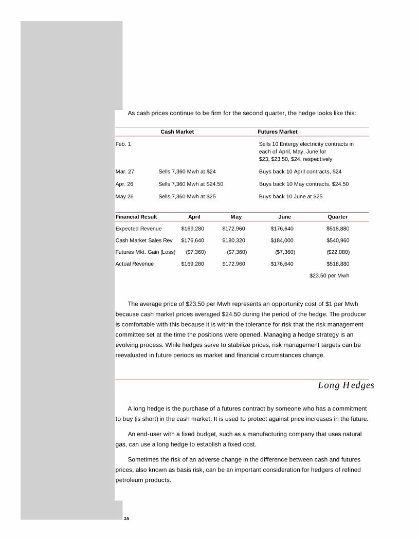
As cash prices continue to be firm for the second quarter, the hedge looks like this:
Cash Market Futures Market
Feb. 1 Sells 10 Entergy electricity contracts in each of April, May, June for $23, $23.50, $24, respectively
Mar. 27 Sells 7,360 Mwh at $24 Buys back 10 April contracts, $24
Apr. 26 Sells 7,360 Mwh at $24.50 Buys back 10 May contracts, $24.50
May 26 Sells 7,360 Mwh at $25 Buys back 10 June at $25
Financial Result April May June Quarter
Expected Revenue $169,280 $172,960 $176,640 $518,880
Cash Market Sales Rev $176,640 $180,320 $184,000 $540,960
Futures Mkt. Gain (Loss) ($7,360) ($7,360) ($7,360) ($22,080)
Actual Revenue $169,280 $172,960 $176,640 $518,880
$23.50 per Mwh
The average price of $23.50 per Mwh represents an opportunity cost of $1 per Mwh
because cash market prices averaged $24.50 during the period of the hedge. The producer
is comfortable with this because it is within the tolerance for risk that the risk management
committee set at the time the positions were opened. Managing a hedge strategy is an
evolving process. While hedges serve to stabilize prices, risk management targets can be
reevaluated in future periods as market and financial circumstances change.
Long Hedges
A long hedge is the purchase of a futures contract by someone who has a commitment
to buy (is short) in the cash market. It is used to protect against price increases in the future.
An end-user with a fixed budget, such as a manufacturing company that uses natural
gas, can use a long hedge to establish a fixed cost.
Sometimes the risk of an adverse change in the difference between cash and futures
prices, also known as basis risk, can be an important consideration for hedgers of refined
petroleum products.
16
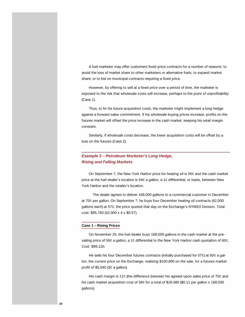
A fuel marketer may offer customers fixed-price contracts for a number of reasons: to
avoid the loss of market share to other marketers or alternative fuels, to expand market
share; or to bid on municipal contracts requiring a fixed price.
However, by offering to sell at a fixed price over a period of time, the marketer is
exposed to the risk that wholesale costs will increase, perhaps to the point of unprofitability
(Case 1).
Thus, to fix his future acquisition costs, the marketer might implement a long hedge
against a forward sales commitment. If his wholesale buying prices increase, profits on the
futures market will offset the price increase in the cash market, keeping his retail margin
constant.
Similarly, if wholesale costs decrease, the lower acquisition costs will be offset by a
loss on the futures (Case 2).
Example 3 – Petroleum Marketer’s Long Hedge,
Rising and Falling Markets
On September 7, the New York Harbor price for heating oil is 55¢ and the cash market
price at the fuel dealer’s location is 54¢ a gallon, a 1¢ differential, or basis, between New
York Harbor and the retailer’s location.
The dealer agrees to deliver 168,000 gallons to a commercial customer in December
at 70¢ per gallon. On September 7, he buys four December heating oil contracts (42,000
gallons each) at 57¢, the price quoted that day on the Exchange’s NYMEX Division. Total
cost: $95,760 (42,000 x 4 x $0.57).
Case 1 – Rising Prices
On November 25, the fuel dealer buys 168,000 gallons in the cash market at the pre-
vailing price of 59¢ a gallon, a 1¢ differential to the New York Harbor cash quotation of 60¢,
Cost: $99,120.
He sells his four December futures contracts (initially purchased for 57¢) at 60¢ a gal-
lon, the current price on the Exchange, realizing $100,800 on the sale, for a futures market
profit of $5,040 (3¢ a gallon).
His cash margin is 11¢ (the difference between his agreed-upon sales price of 70¢ and
his cash market acquisition cost of 59¢ for a total of $18,480 ($0.11 per gallon x 168,000
gallons).

17
Cash Market Futures Market
Sept. 7 Buys four December futures contracts for 57¢ per gallon
Nov. 25 Buys 168,000 gallons Sells four December heating oil futures at 59¢ per gallon for 60¢ per gallon
A cash margin of: $18,480 or 11¢/gallon plus
A futures profit of: $5,040 or 3¢/gallon equals
A total margin of: $23,520 or 14¢/gallon
Case 2 – Falling Prices
On November 25, the dealer buys 168,000 gallons at his local truck loading rack for
49¢ a gallon, the prevailing price on that day, based on the New York Harbor cash quota-
tion of 50¢ a gallon.
He sells his four December futures contracts for 50¢ a gallon, the futures price that
day, realizing $84,000 on the sale, and experiencing a futures loss of $11,760 (7¢ a gallon).
Cash Market Futures Market
Sept. 7 Buy four December heating oil futuresat 57¢ per gallon
Nov. 25 Buys 168,000 gallons Sells four December heating oil futuresfor 49¢ per gallon for 50¢ per gallon
Cash margin of: $35,280 minus
A futures loss of: ($11,760) (7¢/gallon) equals
A total margin of: $23,520 or 14¢/gallon
In summary, the fuel retailer guarantees himself a margin of 14¢ a gallon regardless of
price moves upwards or down in the market.
With the differential between cash and futures stable, as in Cases 1 and 2, spot-price
changes in either direction are the same for both New York and the marketer’s location. As
a result, a decline in the futures price, which causes a loss in the futures market, is offset
cent-for-cent by the increase in the cash margin.

18
Example 4 – Utility Protects Acquisition Costs of Future Wholesale
Purchases Without a Price Commitment From a Seller
On February 1, a utility in Ohio decides that the prices reflected in the futures market
for the second quarter are less expensive than the company’s marginal generating cost. The
utility does not want to wait until the second quarter to buy power because it fears that its
power acquisition costs may move significantly higher than its sales prices. The utility buys
futures contracts for April, May, and June.
Thus, to fix its acquisition costs, the utility might implement a long hedge against its
forward sales. If wholesale buying prices, or production costs, increase, profits on the
futures market will offset the rising costs in the cash market, keeping the retail margin
constant.
Similarly, if wholesale costs decrease, the lower acquisition costs will be offset by a
loss in the futures market.
Case 1 – Rising Prices
On February 1, the utility in Ohio buys 10 Cinergy electricity futures contracts in each of
three months, April, May, and June for $23, $23.50, and $24 per Mwh, respectively. The
cost of the futures purchases are $169,280 for the total April contracts, $172,960 for May,
and $176,640 for June, for a total cost of $518,880 to lock in an average cost of $23.50
per Mwh.
On March 27, the utility buys 7,360 Mwh of its April power requirements in the Cinergy
cash market (neutral basis) for the then prevailing price of $24 per Mwh, and pays $176,640.
That is $7,360 more than it budgeted when it anticipated a price of $23 per Mwh. The utility
also liquidates its futures positions by selling back its 10 April Cinergy futures contracts at
the then-current price of $24 so it doesn’t have to take delivery through the Exchange.
Because nearby futures prices reflect the prevailing cash price, the price of the futures con-
tracts it originally bought for $23 ($169,280), are now worth $24 ($176,640), yielding a gain
in the futures market of $7,360.
The cash market purchase of: $176,640 plus
A futures gain of: $7,360 equals
A net amount of $169,280, or $23 per Mwh, the budgeted sum for April.
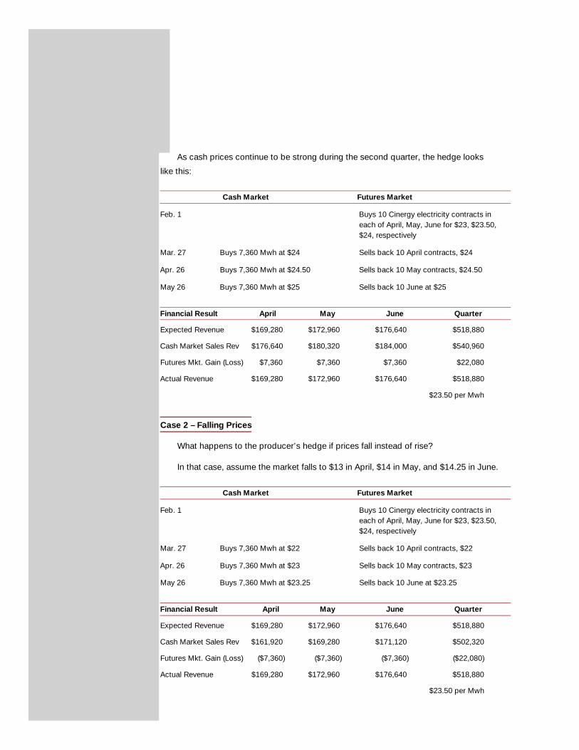
As cash prices continue to be strong during the second quarter, the hedge looks
like this:
Cash Market Futures Market
Feb. 1 Buys 10 Cinergy electricity contracts in each of April, May, June for $23, $23.50, $24, respectively
Mar. 27 Buys 7,360 Mwh at $24 Sells back 10 April contracts, $24
Apr. 26 Buys 7,360 Mwh at $24.50 Sells back 10 May contracts, $24.50
May 26 Buys 7,360 Mwh at $25 Sells back 10 June at $25
Financial Result April May June Quarter
Expected Revenue $169,280 $172,960 $176,640 $518,880
Cash Market Sales Rev $176,640 $180,320 $184,000 $540,960
Futures Mkt. Gain (Loss) $7,360 $7,360 $7,360 $22,080
Actual Revenue $169,280 $172,960 $176,640 $518,880
$23.50 per Mwh
Case 2 – Falling Prices
What happens to the producer’s hedge if prices fall instead of rise?
In that case, assume the market falls to $13 in April, $14 in May, and $14.25 in June.
Cash Market Futures Market
Feb. 1 Buys 10 Cinergy electricity contracts in each of April, May, June for $23, $23.50, $24, respectively
Mar. 27 Buys 7,360 Mwh at $22 Sells back 10 April contracts, $22
Apr. 26 Buys 7,360 Mwh at $23 Sells back 10 May contracts, $23
May 26 Buys 7,360 Mwh at $23.25 Sells back 10 June at $23.25
Financial Result April May June Quarter
Expected Revenue $169,280 $172,960 $176,640 $518,880
Cash Market Sales Rev $161,920 $169,280 $171,120 $502,320
Futures Mkt. Gain (Loss) ($7,360) ($7,360) ($7,360) ($22,080)
Actual Revenue $169,280 $172,960 $176,640 $518,880
$23.50 per Mwh
20
The average acquisition price of $23.50 per Mwh represents an opportunity cost of 75¢
per Mwh because cash market prices averaged $22.75 during the period of the hedge. The
producer is comfortable with this because it is within the tolerance for risk that his risk man-
agement committee set at the time the positions were opened. Managing a hedge strategy is
an ongoing process. While hedges serve to stabilize prices, risk management targets can be
reevaluated in future periods as market and financial circumstances change.
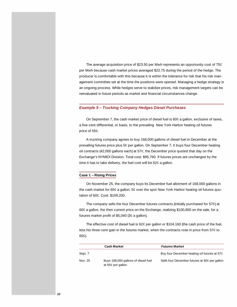
Example 5 – Trucking Company Hedges Diesel Purchases
On September 7, the cash market price of diesel fuel is 60¢ a gallon, exclusive of taxes,
a five-cent differential, or basis, to the prevailing New York Harbor heating oil futures
price of 55¢.
A trucking company agrees to buy 168,000 gallons of diesel fuel in December at the
prevailing futures price plus 5¢ per gallon. On September 7, it buys four December heating
oil contracts (42,000 gallons each) at 57¢, the December price quoted that day on the
Exchange’s NYMEX Division. Total cost: $95,760. If futures prices are unchanged by the
time it has to take delivery, the fuel cost will be 62¢ a gallon.
Case 1 – Rising Prices
On November 25, the company buys its December fuel allotment of 168,000 gallons in
the cash market for 65¢ a gallon, 5¢ over the spot New York Harbor heating oil futures quo-
tation of 60¢. Cost: $109,200.
The company sells the four December futures contracts (initially purchased for 57¢) at
60¢ a gallon, the then current price on the Exchange, realizing $100,800 on the sale, for a
futures market profit of $5,040 (3¢ a gallon).
The effective cost of diesel fuel is 62¢ per gallon or $104,160 (the cash price of the fuel,
less his three-cent gain in the futures market, when the contracts rose in price from 57¢ to
60¢).
Cash Market Futures Market
Sept. 7 Buy four December heating oil futures at 57¢
Nov. 25 Buys 168,000 gallons of diesel fuel Sells four December futures at 60¢ per gallonat 65¢ per gallon
21
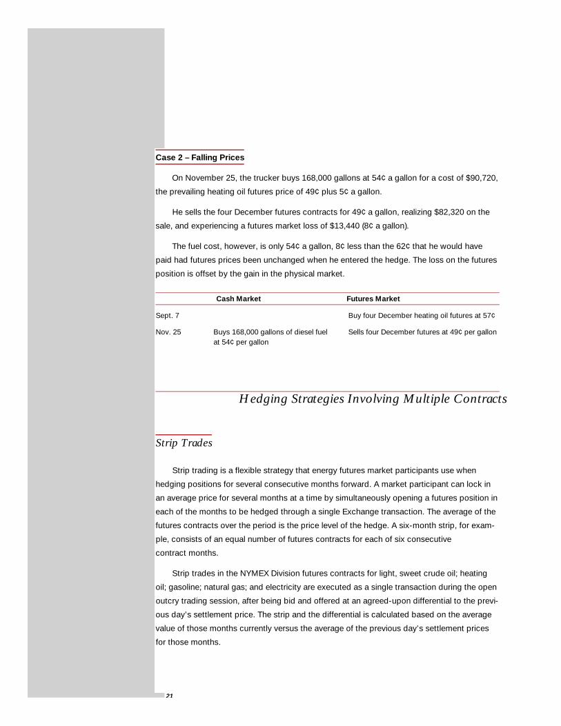
Case 2 – Falling Prices
On November 25, the trucker buys 168,000 gallons at 54¢ a gallon for a cost of $90,720,
the prevailing heating oil futures price of 49¢ plus 5¢ a gallon.
He sells the four December futures contracts for 49¢ a gallon, realizing $82,320 on the
sale, and experiencing a futures market loss of $13,440 (8¢ a gallon).
The fuel cost, however, is only 54¢ a gallon, 8¢ less than the 62¢ that he would have
paid had futures prices been unchanged when he entered the hedge. The loss on the futures
position is offset by the gain in the physical market.
Cash Market Futures Market
Sept. 7 Buy four December heating oil futures at 57¢
Nov. 25 Buys 168,000 gallons of diesel fuel Sells four December futures at 49¢ per gallonat 54¢ per gallon
Hedging Strategies Involving Multiple Contracts
Strip Trades
Strip trading is a flexible strategy that energy futures market participants use when
hedging positions for several consecutive months forward. A market participant can lock in
an average price for several months at a time by simultaneously opening a futures position in
each of the months to be hedged through a single Exchange transaction. The average of the
futures contracts over the period is the price level of the hedge. A six-month strip, for exam-
ple, consists of an equal number of futures contracts for each of six consecutive
contract months.
Strip trades in the NYMEX Division futures contracts for light, sweet crude oil; heating
oil; gasoline; natural gas; and electricity are executed as a single transaction during the open
outcry trading session, after being bid and offered at an agreed-upon differential to the previ-
ous day’s settlement price. The strip and the differential is calculated based on the average
value of those months currently versus the average of the previous day’s settlement prices
for those months.
22
The ability to obtain an average price for multiple months enables a hedger to average
his cash flow over a period of time. Positions can be hedged for as little as two consecutive
months, or can go forward for up to 12 months in unleaded gasoline; 18 months in heating
oil and electricity; 30 months in light, sweet crude oil; and 36 months in Henry Hub natural
gas.
The futures positions assumed in a strip trade are like any other futures position. Any
single month’s position can be liquidated by an offsetting futures trade, an exchange of
futures for physicals (EFP), or, if desired, physical delivery through the Exchange clearing-
house. Strips let a hedger retain the flexibility to change a strategy by buying or selling addi-
tional futures contracts in any month, or liquidating the position of any month of the strip,
something that cannot be done easily with over-the-counter instruments.
Regular margin requirements apply to strip trades. The participant will be required to
post and maintain margin levels for each month in the strip as if it were a separate position.
Example 6 – Petroleum Refiner’s Use Of A Strip Trade
A refiner anticipates the purchase of 60,000 barrels of crude oil, the volume distributed
evenly over a six-month period beginning in October. The use of the strip allows the com-
pany to hedge its expenditures for crude oil evenly throughout the period.
The refiner’s risk management committee is comfortable with locking in this strip’s
price level over the period of their purchases, and, considering their fundamental view of the
crude oil market, is even willing to pay a higher price, if necessary.
The risk manager determines that those months are currently trading at an average that
is 10¢ over the average of the previous day’s settlement price, or $22.35. Assuming he
wishes to hedge 100% of his physical requirements, he buys 10 contracts for each of the
six months, or 60 contracts, representing 60,000 barrels, since each futures contract is for
1,000 barrels.
The refiner’s hedge, which has locked in a price of $22.35 for a total of 60,000 barrels
over the period, looks like this:

23
Month Transaction Price Market Position
OCT $22.54 Long 10 contracts
NOV $22.42 Long 10 contracts
DEC $22.35 Long 10 contracts
JAN $22.29 Long 10 contracts
FEB $22.26 Long 10 contracts
MAR $22.24 Long 10 contracts
Average $22.35
Assuming the refiner takes delivery from its traditional suppliers, it will liquidate the
futures positions in the relevant months, offsetting its physical market transactions. If the
refiner chooses, however, it can take delivery through the Exchange for any, or all, of the
months involved in the strategy.
As with any other hedge, there may be a loss in the futures market for a particular
month that is compensated for by a gain in the cash market, conversely a gain in the
futures market will offset a loss in the cash market.
Regular margin requirements apply to strip trades. The participant will be required to
post and maintain margin levels for each month in the strip as if it were a separate position.
Example 7 – Petroleum Marketer’s Long Hedge; Guaranteeing
Retail Prices by Purchasing a “Strip” of Futures
By allowing market participants to lock in an average price over a period of time, strip
trading strategies can be used by vendors of refined products to offer their customers sea-
sonal price stability through fixed-price programs. These programs have become increas-
ingly popular with heating oil retailers who are faced with increasingly competitive market
conditions, and their customers, who desire stable pricing, thus avoiding the price spikes
that can wreak havoc with household budgets.
Retailers are able to offer seasonal fixed pricing with minimal risk to their operating
margins by locking-in ahead of time during the off-season the price required to service
customers during the winter. This can be accomplished with strips of NYMEX Division heat-
ing oil futures contracts.
A retailer who wants to offer a fixed price program would in the spring and summer
solicit as many customers as possible whose consumption averages 1,000 gallons each
24
over the period from October to the beginning of April, with the bulk of consumption occur-
ring during December, January, and February.
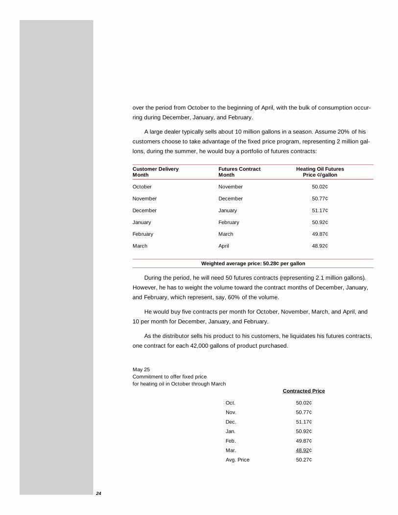
A large dealer typically sells about 10 million gallons in a season. Assume 20% of his
customers choose to take advantage of the fixed price program, representing 2 million gal-
lons, during the summer, he would buy a portfolio of futures contracts:
Customer Delivery Futures Contract Heating Oil FuturesMonth Month Price ¢/gallon
October November 50.02¢
November December 50.77¢
December January 51.17¢
January February 50.92¢
February March 49.87¢
March April 48.92¢
Weighted average price: 50.28¢ per gallon
During the period, he will need 50 futures contracts (representing 2.1 million gallons).
However, he has to weight the volume toward the contract months of December, January,
and February, which represent, say, 60% of the volume.
He would buy five contracts per month for October, November, March, and April, and
10 per month for December, January, and February.
As the distributor sells his product to his customers, he liquidates his futures contracts,
one contract for each 42,000 gallons of product purchased.
May 25 Commitment to offer fixed price for heating oil in October through March
Contracted Price
Oct. 50.02¢
Nov. 50.77¢
Dec. 51.17¢
Jan. 50.92¢
Feb. 49.87¢
Mar. 48.92¢
Avg. Price 50.27¢
25
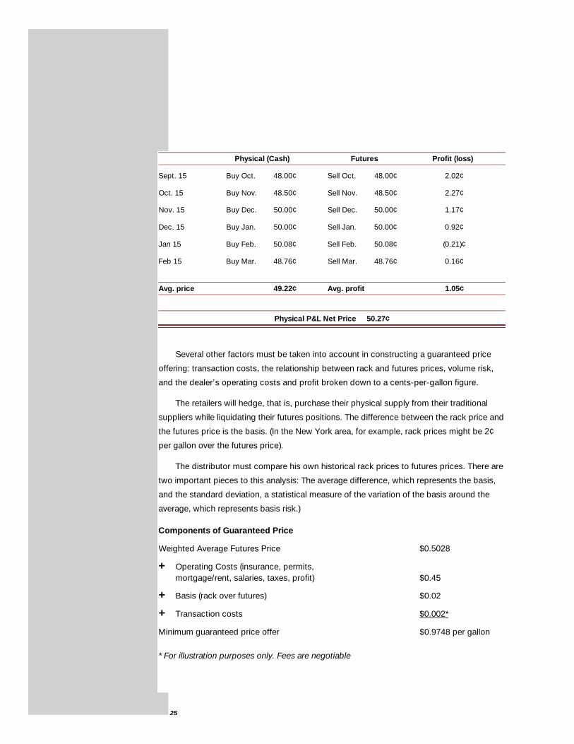
Physical (Cash) Futures Profit (loss)
Sept. 15 Buy Oct. 48.00¢ Sell Oct. 48.00¢ 2.02¢
Oct. 15 Buy Nov. 48.50¢ Sell Nov. 48.50¢ 2.27¢
Nov. 15 Buy Dec. 50.00¢ Sell Dec. 50.00¢ 1.17¢
Dec. 15 Buy Jan. 50.00¢ Sell Jan. 50.00¢ 0.92¢
Jan 15 Buy Feb. 50.08¢ Sell Feb. 50.08¢ (0.21)¢
Feb 15 Buy Mar. 48.76¢ Sell Mar. 48.76¢ 0.16¢
Avg. price 49.22¢ Avg. profit 1.05¢
Physical P&L Net Price 50.27¢
Several other factors must be taken into account in constructing a guaranteed price
offering: transaction costs, the relationship between rack and futures prices, volume risk,
and the dealer’s operating costs and profit broken down to a cents-per-gallon figure.
The retailers will hedge, that is, purchase their physical supply from their traditional
suppliers while liquidating their futures positions. The difference between the rack price and
the futures price is the basis. (In the New York area, for example, rack prices might be 2¢
per gallon over the futures price).
The distributor must compare his own historical rack prices to futures prices. There are
two important pieces to this analysis: The average difference, which represents the basis,
and the standard deviation, a statistical measure of the variation of the basis around the
average, which represents basis risk.)
Components of Guaranteed Price
Weighted Average Futures Price $0.5028
+ Operating Costs (insurance, permits, mortgage/rent, salaries, taxes, profit) $0.45
+ Basis (rack over futures) $0.02
+ Transaction costs $0.002*
Minimum guaranteed price offer $0.9748 per gallon
* For illustration purposes only. Fees are negotiable

26
Spread Trades
Spread positions offer another way of using futures. There are many types of spreads,
but they all have two things in common. First, a spread always involves at least two futures
positions, which are maintained simultaneously. For example, a trader may be long 10 June
electricity contracts and short 10 September electricity contracts. Second, the price
changes in the two or more legs of the position are expected to have a reasonably pre-
dictable relationship, and the potential profitability of the spread lies in that relationship or
expected changes to that relationship. For example, the trader who is long 10 June con-
tracts (the near-term contract) and short 10 September contracts (the distant contract) will
benefit if market forces cause the near-term contract to make a larger advance than the
more distant contract – or if market forces cause the distant contract to drop more sharply
than the near-term contract.
Crack Spreads
A petroleum refiner, like most manufacturers, is caught between two markets: the raw
materials he has to purchase and the finished products he offers for sale. It is the nature of
these markets for prices to be independently subject to variables of supply, demand, trans-
portation, and other factors. This can put refiners at enormous risk when crude oil prices
rise while refined product prices stay static or even decline, thus narrowing the spread.
The Exchange facilitates crack spread trading by treating them as a single transaction
for the purpose of determining a market participant’s margin requirement.
To calculate the theoretical refining margin, first calculate the combined value of gaso-
line and heating oil, then compare the combined value to the price of crude. Since crude oil
is quoted in dollars per barrel and the products are quoted in cents per gallon, heating oil
and gasoline prices must be converted to dollars per barrel by multiplying the cents per gal-
lon price by 42 (there are 42 gallons in a barrel). If the combined value of the products is
higher than the price of the crude, the gross cracking margin is positive. Conversely, if the
combined value of the products is less than that of crude, then the cracking margin is
negative.
Using a ratio of two crude oil contracts to one gasoline contract plus one heating oil
contract, the gross cracking margin is calculated as follows:
27
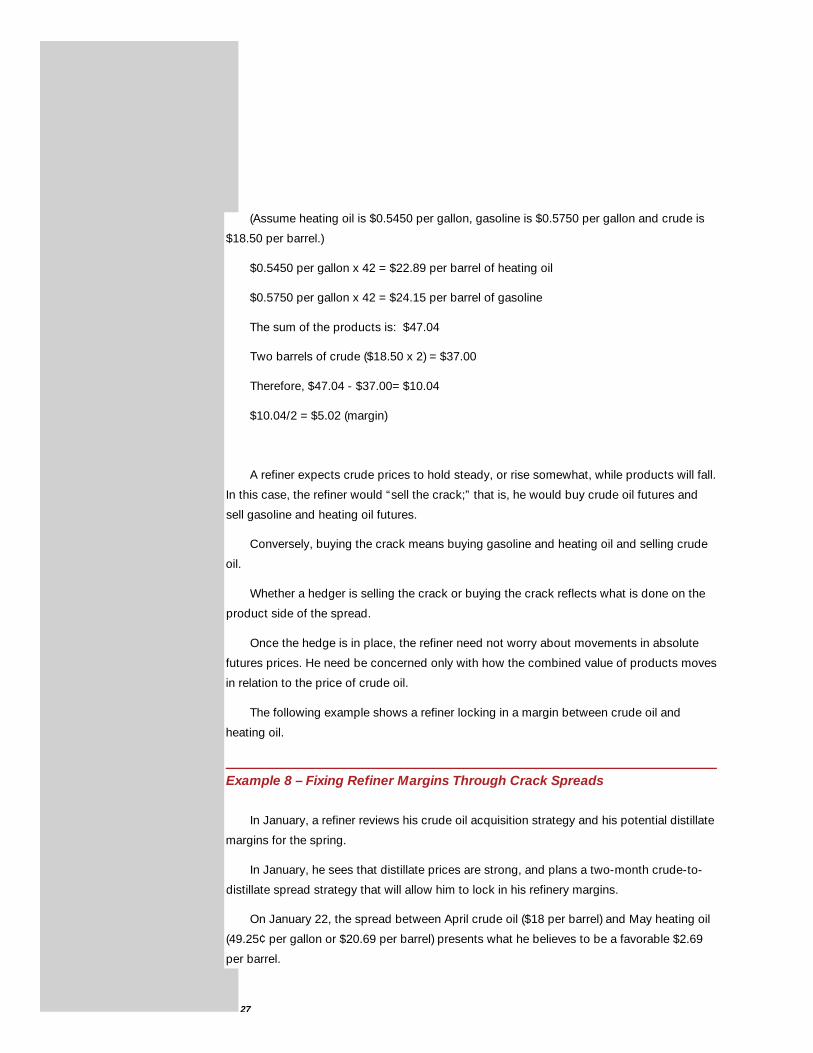
(Assume heating oil is $0.5450 per gallon, gasoline is $0.5750 per gallon and crude is
$18.50 per barrel.)
$0.5450 per gallon x 42 = $22.89 per barrel of heating oil
$0.5750 per gallon x 42 = $24.15 per barrel of gasoline
The sum of the products is: $47.04
Two barrels of crude ($18.50 x 2) = $37.00
Therefore, $47.04 - $37.00= $10.04
$10.04/2 = $5.02 (margin)
A refiner expects crude prices to hold steady, or rise somewhat, while products will fall.
In this case, the refiner would “sell the crack;” that is, he would buy crude oil futures and
sell gasoline and heating oil futures.
Conversely, buying the crack means buying gasoline and heating oil and selling crude
oil.
Whether a hedger is selling the crack or buying the crack reflects what is done on the
product side of the spread.
Once the hedge is in place, the refiner need not worry about movements in absolute
futures prices. He need be concerned only with how the combined value of products moves
in relation to the price of crude oil.
The following example shows a refiner locking in a margin between crude oil and
heating oil.
Example 8 – Fixing Refiner Margins Through Crack Spreads
In January, a refiner reviews his crude oil acquisition strategy and his potential distillate
margins for the spring.
In January, he sees that distillate prices are strong, and plans a two-month crude-to-
distillate spread strategy that will allow him to lock in his refinery margins.
On January 22, the spread between April crude oil ($18 per barrel) and May heating oil
(49.25¢ per gallon or $20.69 per barrel) presents what he believes to be a favorable $2.69
per barrel.
28
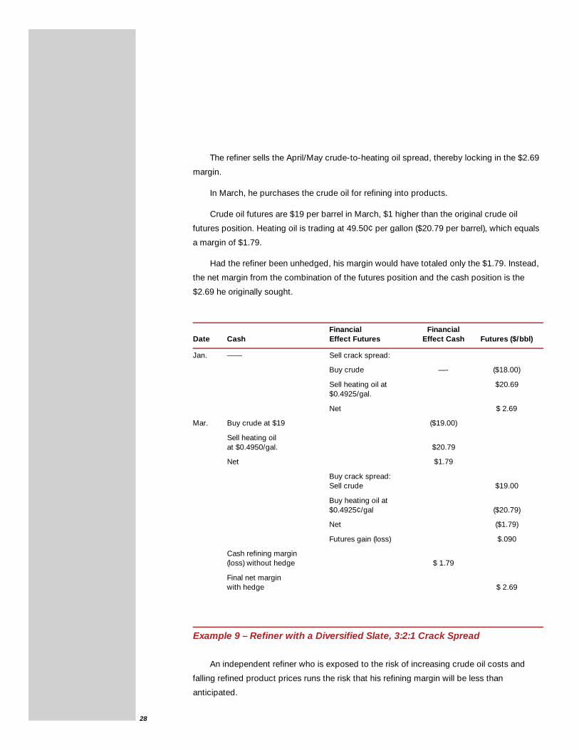
The refiner sells the April/May crude-to-heating oil spread, thereby locking in the $2.69
margin.
In March, he purchases the crude oil for refining into products.
Crude oil futures are $19 per barrel in March, $1 higher than the original crude oil
futures position. Heating oil is trading at 49.50¢ per gallon ($20.79 per barrel), which equals
a margin of $1.79.
Had the refiner been unhedged, his margin would have totaled only the $1.79. Instead,
the net margin from the combination of the futures position and the cash position is the
$2.69 he originally sought.
Financial FinancialDate Cash Effect Futures Effect Cash Futures ($/bbl)
Jan. —— Sell crack spread:
Buy crude —- ($18.00)
Sell heating oil at $20.69$0.4925/gal.
Net $ 2.69
Mar. Buy crude at $19 ($19.00)
Sell heating oil at $0.4950/gal. $20.79
Net $1.79
Buy crack spread:Sell crude $19.00
Buy heating oil at$0.4925¢/gal ($20.79)
Net ($1.79)
Futures gain (loss) $.090
Cash refining margin (loss) without hedge $ 1.79
Final net marginwith hedge $ 2.69
Example 9 – Refiner with a Diversified Slate, 3:2:1 Crack Spread
An independent refiner who is exposed to the risk of increasing crude oil costs and
falling refined product prices runs the risk that his refining margin will be less than
anticipated.

29
The refiner initiates a long hedge in crude oil and short hedges in heating oil and gaso-
line to fix a substantial portion of his refining margin.
On September 15, the refiner incurs an obligation to buy 6,000 barrels of crude oil on
May 16 at prevailing cash prices. He is also obliged to sell 84,000 gallons (2,000 barrels) of
heating oil and 168,000 gallons (4,000 barrels) of gasoline on November 28 at prevailing
spot prices.
The crack spread has ensured that refining crude oil will be at least as profitable in
November as it was in September, regardless of whether the actual cash margin narrows or
widens. A decline in the cash margin is offset by a gain in the futures market; conversely,
any gain in the cash market is offset by a loss in the futures market. The example assumes a
crack spread of three crude oil, two gasoline, one heating oil.
Date Prices Action Futures Market
Sept. 15 Sweet crude: Agrees to buy at prevailing Buys six Nov. sweet crudeCushing — $18.90 prices: 6,000 bbl. sweet contracts at $18.45/bbl.
crude on Oct. 16Heating Oil:
Gulf Coast, Commits to sell at $0.4875/gal, prevailing prices:$20.47/bbl 84,000 gal. heating oil on Sells two Dec. heating oil
Nov. 28 contracts, $.5255/gal,$22.07/bbl
N.Y. Harbor, $0.5125/gal, $21.52/bbl
Gasoline: Commits to sell at prevailing prices:168,000 gal. gasoline Sells four Dec. New Yorkon Nov. 28 Harbor gasoline contracts,
$0.5275/gal, $22.15/bbl
Gulf Coast, $0.5450/gal, $22.89/bbl
N.Y. Harbor, $0.5850/gal, $24.57/bbl
Gulf Coast cash margin: (6 x $18.90)-[(2 x $20.47)+(4 x $22.89)]/6 = $3.18/bbl.
Cushing/NY Harbor cash margin: [[(2 x $21.52)+(4 x $24.57)]-(6 x $18.90)]/6 = $4.65/bbl.
Crack spread: [[(2 x $22.07)+(4 x $22.15)]-(6 x $18.45)]/6 = $3.67
Cash basis - $1.47/bbl ($3.18-$4.65) Futures Crack Spread:
Expected margin $2.20/bbl ($3.67-$1.47) $3.67/bbl.
30
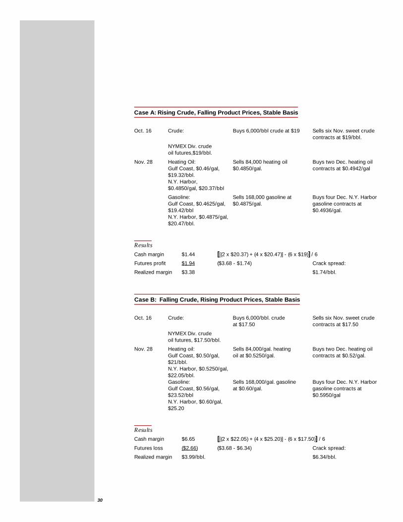
Case A: Rising Crude, Falling Product Prices, Stable Basis
Oct. 16 Crude: Buys 6,000/bbl crude at $19 Sells six Nov. sweet crudecontracts at $19/bbl.
NYMEX Div. crudeoil futures,$19/bbl.
Nov. 28 Heating Oil: Sells 84,000 heating oil Buys two Dec. heating oil Gulf Coast, $0.46/gal, $0.4850/gal. contracts at $0.4942/gal$19.32/bbl.N.Y. Harbor, $0.4850/gal, $20.37/bbl
Gasoline: Sells 168,000 gasoline at Buys four Dec. N.Y. HarborGulf Coast, $0.4625/gal, $0.4875/gal. gasoline contracts at $19.42/bbl $0.4936/gal.N.Y. Harbor, $0.4875/gal, $20.47/bbl.
Results
Cash margin $1.44 [[(2 x $20.37) + (4 x $20.47)] - (6 x $19)] / 6
Futures profit $1.94 ($3.68 - $1.74) Crack spread:
Realized margin $3.38 $1.74/bbl.
Case B: Falling Crude, Rising Product Prices, Stable Basis
Oct. 16 Crude: Buys 6,000/bbl. crude Sells six Nov. sweet crudeat $17.50 contracts at $17.50
NYMEX Div. crude oil futures, $17.50/bbl.
Nov. 28 Heating oil: Sells 84,000/gal. heating Buys two Dec. heating oilGulf Coast, $0.50/gal, oil at $0.5250/gal. contracts at $0.52/gal.$21/bbl.N.Y. Harbor, $0.5250/gal, $22.05/bbl.Gasoline: Sells 168,000/gal. gasoline Buys four Dec. N.Y. HarborGulf Coast, $0.56/gal, at $0.60/gal. gasoline contracts at$23.52/bbl $0.5950/galN.Y. Harbor, $0.60/gal, $25.20
Results
Cash margin $6.65 [[(2 x $22.05) + (4 x $25.20)] - (6 x $17.50)] / 6
Futures loss ($2.66) ($3.68 - $6.34) Crack spread:
Realized margin $3.99/bbl. $6.34/bbl.

31
Timing risk and basis risk can be quantified and are usually less than the absolute price
risk to which the refiner is subjected.
The example assumes fixed points in time of obligation to buy and sell in the cash mar-
ket. In practice, these may not be entirely known or fixed.
Purchasing a Crack Spread
The purchase of a crack spread is the opposite of the crack spread hedge. It entails a
short hedge in crude oil and long hedges in products. Refiners are naturally long the crack
spread as they buy crude and sell products. At times, however, refiners do the opposite,
they buy products and sell crude and thus find purchasing a crack spread a useful strategy.
When refiners are forced to shut down for repairs, they often have to enter the crude oil
and product markets to honor existing purchase and supply contracts. Unable to produce
enough products to meet term supply obligations, the refiner must buy products at spot
prices for resale to his term customers. Furthermore, lacking adequate storage space for
incoming supplies of crude oil, the refiner must sell the excess on the spot market.
If the refiner’s supply and sales commitments are substantial and if he is forced to
make an unplanned entry into the spot market, it is possible that prices might move against
him. To protect himself from increasing product prices and decreasing crude oil prices, the
refiner uses a short hedge against crude oil and a long hedge against products.
Spark Spreads
Similar to the crack spread, the “spark spread” has developed in the electricity markets
as an intermarket spread for electricity and natural gas. The spark spread involves the
simultaneous purchase and sale of electricity and natural gas futures contracts. This allows
traders to take advantage of the generic conversions of natural gas to power to help price
the forward electric power curve using natural gas-fired generation operating efficiencies
and prices.
The regions with the most transparent short-term natural gas to power price correlation
typically have been the northwestern and southwestern United States and Texas. These
areas coincide with the Palo Verde and COB electric power futures contracts trading on the
Exchange.
The gas to power correlation is not as good in other parts of the country where coal,
oil, or nuclear are predominantly used on the margin.
32
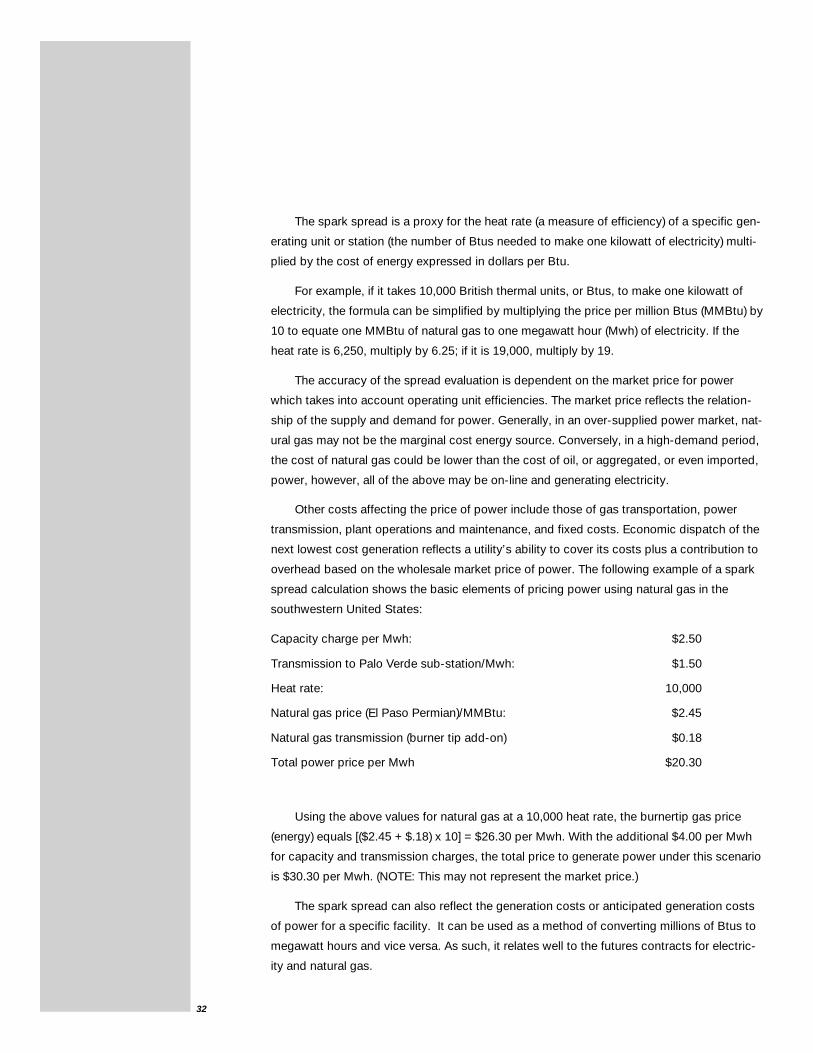
The spark spread is a proxy for the heat rate (a measure of efficiency) of a specific gen-
erating unit or station (the number of Btus needed to make one kilowatt of electricity) multi-
plied by the cost of energy expressed in dollars per Btu.
For example, if it takes 10,000 British thermal units, or Btus, to make one kilowatt of
electricity, the formula can be simplified by multiplying the price per million Btus (MMBtu) by
10 to equate one MMBtu of natural gas to one megawatt hour (Mwh) of electricity. If the
heat rate is 6,250, multiply by 6.25; if it is 19,000, multiply by 19.
The accuracy of the spread evaluation is dependent on the market price for power
which takes into account operating unit efficiencies. The market price reflects the relation-
ship of the supply and demand for power. Generally, in an over-supplied power market, nat-
ural gas may not be the marginal cost energy source. Conversely, in a high-demand period,
the cost of natural gas could be lower than the cost of oil, or aggregated, or even imported,
power, however, all of the above may be on-line and generating electricity.
Other costs affecting the price of power include those of gas transportation, power
transmission, plant operations and maintenance, and fixed costs. Economic dispatch of the
next lowest cost generation reflects a utility’s ability to cover its costs plus a contribution to
overhead based on the wholesale market price of power. The following example of a spark
spread calculation shows the basic elements of pricing power using natural gas in the
southwestern United States:
Capacity charge per Mwh: $2.50
Transmission to Palo Verde sub-station/Mwh: $1.50
Heat rate: 10,000
Natural gas price (El Paso Permian)/MMBtu: $2.45
Natural gas transmission (burner tip add-on) $0.18
Total power price per Mwh $20.30
Using the above values for natural gas at a 10,000 heat rate, the burnertip gas price
(energy) equals [($2.45 + $.18) x 10] = $26.30 per Mwh. With the additional $4.00 per Mwh
for capacity and transmission charges, the total price to generate power under this scenario
is $30.30 per Mwh. (NOTE: This may not represent the market price.)
The spark spread can also reflect the generation costs or anticipated generation costs
of power for a specific facility. It can be used as a method of converting millions of Btus to
megawatt hours and vice versa. As such, it relates well to the futures contracts for electric-
ity and natural gas.
33
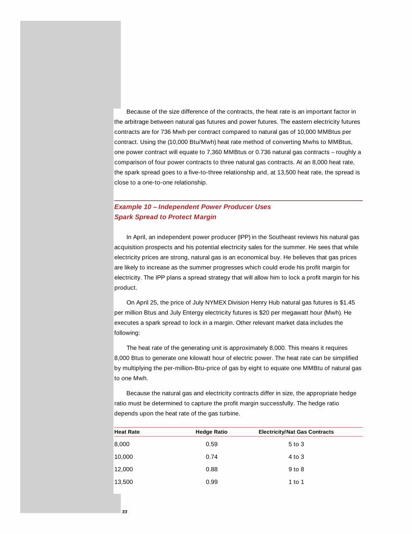
Because of the size difference of the contracts, the heat rate is an important factor in
the arbitrage between natural gas futures and power futures. The eastern electricity futures
contracts are for 736 Mwh per contract compared to natural gas of 10,000 MMBtus per
contract. Using the (10,000 Btu/Mwh) heat rate method of converting Mwhs to MMBtus,
one power contract will equate to 7,360 MMBtus or 0.736 natural gas contracts – roughly a
comparison of four power contracts to three natural gas contracts. At an 8,000 heat rate,
the spark spread goes to a five-to-three relationship and, at 13,500 heat rate, the spread is
close to a one-to-one relationship.
Example 10 – Independent Power Producer Uses
Spark Spread to Protect Margin
In April, an independent power producer (IPP) in the Southeast reviews his natural gas
acquisition prospects and his potential electricity sales for the summer. He sees that while
electricity prices are strong, natural gas is an economical buy. He believes that gas prices
are likely to increase as the summer progresses which could erode his profit margin for
electricity. The IPP plans a spread strategy that will allow him to lock a profit margin for his
product.
On April 25, the price of July NYMEX Division Henry Hub natural gas futures is $1.45
per million Btus and July Entergy electricity futures is $20 per megawatt hour (Mwh). He
executes a spark spread to lock in a margin. Other relevant market data includes the
following:
The heat rate of the generating unit is approximately 8,000. This means it requires
8,000 Btus to generate one kilowatt hour of electric power. The heat rate can be simplified
by multiplying the per-million-Btu-price of gas by eight to equate one MMBtu of natural gas
to one Mwh.
Because the natural gas and electricity contracts differ in size, the appropriate hedge
ratio must be determined to capture the profit margin successfully. The hedge ratio
depends upon the heat rate of the gas turbine.
Heat Rate Hedge Ratio Electricity/Nat Gas Contracts
8,000 0.59 5 to 3
10,000 0.74 4 to 3
12,000 0.88 9 to 8
13,500 0.99 1 to 1
34
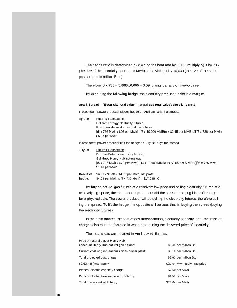
The hedge ratio is determined by dividing the heat rate by 1,000, multiplying it by 736
(the size of the electricity contract in Mwh) and dividing it by 10,000 (the size of the natural
gas contract in million Btus).
Therefore, 8 x 736 = 5,888/10,000 = 0.59, giving it a ratio of five-to-three.
By executing the following hedge, the electricity producer locks in a margin:
Spark Spread = [Electricity total value - natural gas total value]/electricity units
Independent power producer places hedge on April 25, sells the spread:
Apr. 25 Futures TransactionSell five Entergy electricity futuresBuy three Henry Hub natural gas futures[(5 x 736 Mwh x $26 per Mwh) - (3 x 10,000 MMBtu x $2.45 per MMBtu)]/(5 x 736 per Mwh)$6.03 per Mwh
Independent power producer lifts the hedge on July 28, buys the spread
July 28 Futures TransactionBuy five Entergy electricity futuresSell three Henry Hub natural gas[(5 x 736 Mwh x $23 per Mwh) - (3 x 10,000 MMBtu x $2.65 per MMBtu)]/(5 x 736 Mwh)$1.40 per Mwh
Result of $6.03 - $1.40 = $4.63 per Mwh, net profithedge: $4.63 per Mwh x (5 x 736 Mwh) = $17,038.40
By buying natural gas futures at a relatively low price and selling electricity futures at a
relatively high price, the independent producer sold the spread, hedging his profit margin
for a physical sale. The power producer will be selling the electricity futures, therefore sell-
ing the spread. To lift the hedge, the opposite will be true, that is, buying the spread (buying
the electricity futures).
In the cash market, the cost of gas transportation, electricity capacity, and transmission
charges also must be factored in when determining the delivered price of electricity.
The natural gas cash market in April looked like this:
Price of natural gas at Henry Hubbased on Henry Hub natural gas futures: $2.45 per million Btu
Current cost of gas transmission to power plant: $0.18 per million Btu
Total projected cost of gas $2.63 per million Btu
$2.63 x 8 (heat rate) = $21.04 Mwh equiv. gas price
Present electric capacity charge $2.50 per Mwh
Present electric transmission to Entergy $1.50 per Mwh
Total power cost at Entergy $25.04 per Mwh
35
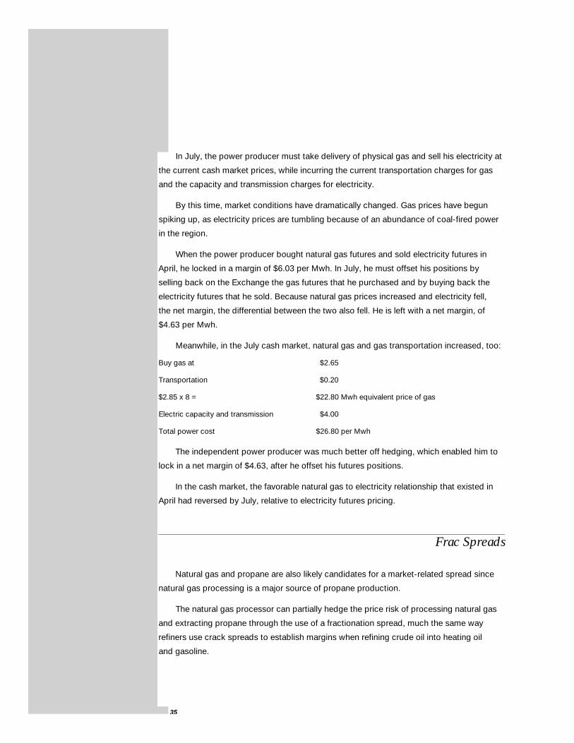
In July, the power producer must take delivery of physical gas and sell his electricity at
the current cash market prices, while incurring the current transportation charges for gas
and the capacity and transmission charges for electricity.
By this time, market conditions have dramatically changed. Gas prices have begun
spiking up, as electricity prices are tumbling because of an abundance of coal-fired power
in the region.
When the power producer bought natural gas futures and sold electricity futures in
April, he locked in a margin of $6.03 per Mwh. In July, he must offset his positions by
selling back on the Exchange the gas futures that he purchased and by buying back the
electricity futures that he sold. Because natural gas prices increased and electricity fell,
the net margin, the differential between the two also fell. He is left with a net margin, of
$4.63 per Mwh.
Meanwhile, in the July cash market, natural gas and gas transportation increased, too:
Buy gas at $2.65
Transportation $0.20
$2.85 x 8 = $22.80 Mwh equivalent price of gas
Electric capacity and transmission $4.00
Total power cost $26.80 per Mwh
The independent power producer was much better off hedging, which enabled him to
lock in a net margin of $4.63, after he offset his futures positions.
In the cash market, the favorable natural gas to electricity relationship that existed in
April had reversed by July, relative to electricity futures pricing.
Frac Spreads
Natural gas and propane are also likely candidates for a market-related spread since
natural gas processing is a major source of propane production.
The natural gas processor can partially hedge the price risk of processing natural gas
and extracting propane through the use of a fractionation spread, much the same way
refiners use crack spreads to establish margins when refining crude oil into heating oil
and gasoline.

36
Balancing the Frac Spread by Equating Heating Value
The frac spread is quoted in heating value terms, dollars per million British thermal units
(MMBtu), to equate propane to natural gas. The natural gas futures contract is composed of
10,000 MMBtu, and is quoted in dollars and cents per MMBtu.
Propane is quoted in cents per gallon. One gallon in gaseous form contains approxi-
mately 91,500 Btus. Dividing the price of propane by 0.0915 gives the equivalent price per
MMBtu. If propane were trading at 35¢ per gallon, the cost would be $3.825 per MMBtu.
One propane futures contract, 42,000 gallons, represents about 38% of the heating
value of one natural gas contract of 10,000 MMBtu. The two most popular ratios used to
create a balance heating value position are a 3:1 or 5:2 propane to natural gas spread.
Once the price of propane, quoted in dollars per gallon, has been converted into the
price per MMBtu, the frac spread can be calculated by subtracting the price of natural gas
from the calculated value of propane to yield the gross manufacturing margin. At this point,
the fractionator has only paid for the value of natural gas consumed, or reduced, in pro-
cessing. There are many additional costs including processing, transportation, fractionation,
and marketing that must be paid out of the gross manufacturing margin.
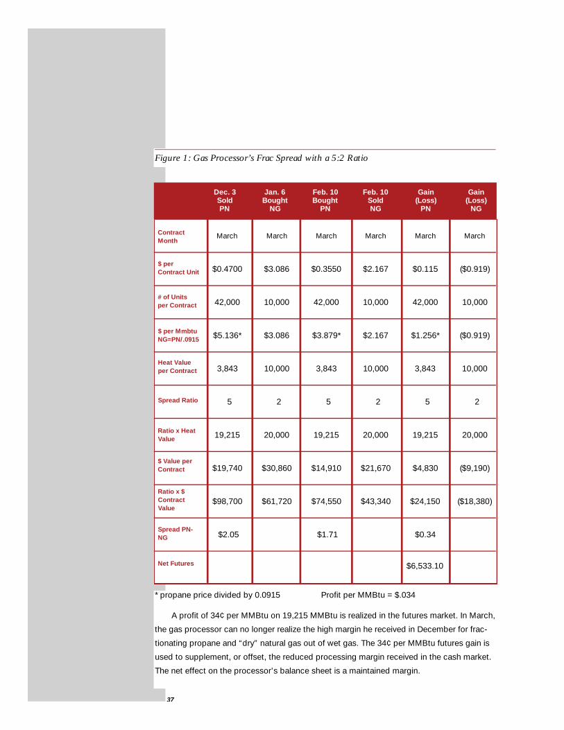
Example 11 – Gas Processors Frac Spread with a 5:2 Ratio
Assume propane futures are trading at 47¢ per gallon ($5.136 per MMBtu). If natural
gas futures were trading at $3.086 per MMBtu, then the frac spread would have a positive
margin of $2.05. From this margin, other operating costs could be covered.
The most frequent application of frac spreads is found among gas processors. In the
example below, a processor wishes to lock in the $2.05 per MMBtu spread between the
two products for the March contract. He enters into the market on December 3, and liqui-
dates his position on February 10, several days before the March contract ceases trading.
37
Figure 1: Gas Processor’s Frac Spread with a 5:2 Ratio
Dec. 3SoldPN
Jan. 6Bought
NG
Feb. 10Bought
PN
Feb. 10SoldNG
Gain(Loss)
PN
Gain(Loss)
NG
March March March March March March
$0.4700 $3.086 $0.3550 $2.167 $0.115 ($0.919)
42,000 10,000 42,000 10,000 42,000 10,000
$5.136* $3.086 $3.879* $2.167 $1.256* ($0.919)
3,843 10,000 3,843 10,000 3,843 10,000
5 2 5 2 5 2
19,215 20,000 19,215 20,000 19,215 20,000
$19,740 $30,860 $14,910 $21,670 $4,830 ($9,190)
$98,700 $61,720 $74,550 $43,340 $24,150 ($18,380)
$2.05 $1.71 $0.34
$6,533.10
ContractMonth
$ perContract Unit
# of Units per Contract
$ per Mmbtu NG=PN/.0915
Heat Valueper Contract
Spread Ratio
Ratio x HeatValue
$ Value perContract
Ratio x $ContractValue
Spread PN-NG
Net Futures
* propane price divided by 0.0915 Profit per MMBtu = $.034
A profit of 34¢ per MMBtu on 19,215 MMBtu is realized in the futures market. In March,
the gas processor can no longer realize the high margin he received in December for frac-
tionating propane and “dry” natural gas out of wet gas. The 34¢ per MMBtu futures gain is
used to supplement, or offset, the reduced processing margin received in the cash market.
The net effect on the processor’s balance sheet is a maintained margin.
38
If the frac spread had increased beyond $2.05 instead of decreasing, the processor
would have lost an opportunity for further gain but, as a hedger, he was content in locking
in the $2.05 per MMBtu margin. He was willing to forego a potentially higher margin in
exchange for eliminating the chance of a lower margin.
39
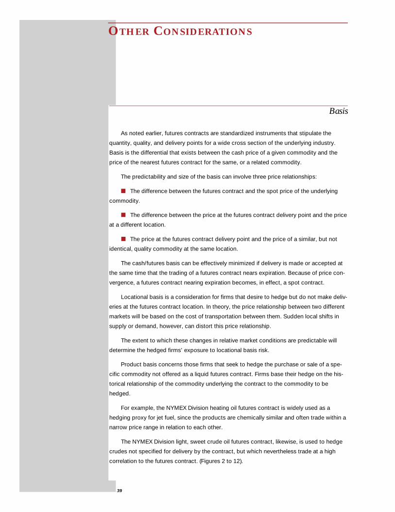
OTHER CONSIDERATIONS
Basis
As noted earlier, futures contracts are standardized instruments that stipulate the
quantity, quality, and delivery points for a wide cross section of the underlying industry.
Basis is the differential that exists between the cash price of a given commodity and the
price of the nearest futures contract for the same, or a related commodity.
The predictability and size of the basis can involve three price relationships:
■ The difference between the futures contract and the spot price of the underlying
commodity.
■ The difference between the price at the futures contract delivery point and the price
at a different location.
■ The price at the futures contract delivery point and the price of a similar, but not
identical, quality commodity at the same location.
The cash/futures basis can be effectively minimized if delivery is made or accepted at
the same time that the trading of a futures contract nears expiration. Because of price con-
vergence, a futures contract nearing expiration becomes, in effect, a spot contract.
Locational basis is a consideration for firms that desire to hedge but do not make deliv-
eries at the futures contract location. In theory, the price relationship between two different
markets will be based on the cost of transportation between them. Sudden local shifts in
supply or demand, however, can distort this price relationship.
The extent to which these changes in relative market conditions are predictable will
determine the hedged firms’ exposure to locational basis risk.
Product basis concerns those firms that seek to hedge the purchase or sale of a spe-
cific commodity not offered as a liquid futures contract. Firms base their hedge on the his-
torical relationship of the commodity underlying the contract to the commodity to be
hedged.
For example, the NYMEX Division heating oil futures contract is widely used as a
hedging proxy for jet fuel, since the products are chemically similar and often trade within a
narrow price range in relation to each other.
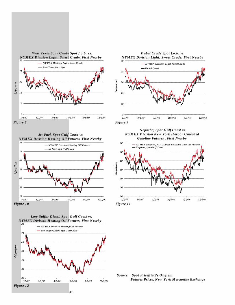
The NYMEX Division light, sweet crude oil futures contract, likewise, is used to hedge
crudes not specified for delivery by the contract, but which nevertheless trade at a high
correlation to the futures contract. (Figures 2 to 12).

West Texas Intermediate Spot Cushing vs.
NYMEX Division Light, Sweet Crude, First Nearby
Figure 2
Bonny Light Spot vs.
NYMEX Division Light, Sweet Crude, First Nearby
Unleaded Gasoline, Spot N.Y. Barge vs.
NYMEX Division NY Harbor Unleaded Gasoline
Futures, First Nearby
Figure 6
Light Louisiana Sweet, f.o.b. St. James, vs.
NYMEX Division Light, Sweet Crude, First Nearby
Figure 3
No. 2 Heating Oil, Spot N.Y. Barge vs.
NYMEX Division Heating Oil Futures, First Nearby
Figure 5
Northwest Europe Gasoil vs.
NYMEX Division Heating Oil Futures, First Nearby
Figure 7
Figure 4
41
West Texas Sour Crude Spot f.o.b. vs.
NYMEX Division Light, Sweet Crude, First Nearby
Figure 8
Jet Fuel, Spot Gulf Coast vs.
NYMEX Division Heating Oil Futures, First Nearby
Figure 10
Dubai Crude Spot f.o.b. vs.
NYMEX Division Light, Sweet Crude, First Nearby
Figure 9
Naphtha, Spot Gulf Coast vs.
NYMEX Division New York Harbor Unleaded
Gasoline Futures , First Nearby
Figure 11
Low Sulfur Diesel, Spot Gulf Coast vs.
NYMEX Division Heating Oil Futures, First Nearby
Figure 12
Source: Spot Prices, Platt’s Oilgram
Futures Prices, New York Mercantile Exchange
42
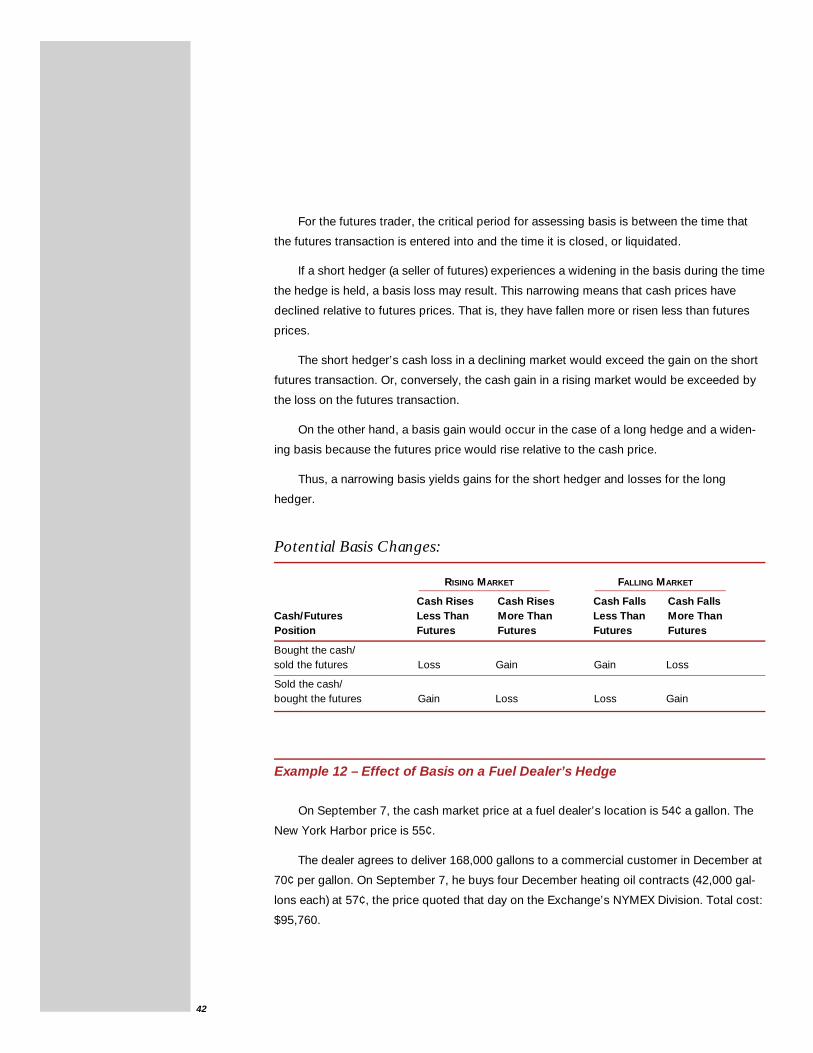
For the futures trader, the critical period for assessing basis is between the time that
the futures transaction is entered into and the time it is closed, or liquidated.
If a short hedger (a seller of futures) experiences a widening in the basis during the time
the hedge is held, a basis loss may result. This narrowing means that cash prices have
declined relative to futures prices. That is, they have fallen more or risen less than futures
prices.
The short hedger’s cash loss in a declining market would exceed the gain on the short
futures transaction. Or, conversely, the cash gain in a rising market would be exceeded by
the loss on the futures transaction.
On the other hand, a basis gain would occur in the case of a long hedge and a widen-
ing basis because the futures price would rise relative to the cash price.
Thus, a narrowing basis yields gains for the short hedger and losses for the long
hedger.
Potential Basis Changes:
RISING MARKET FALLING MARKET
Cash Rises Cash Rises Cash Falls Cash FallsCash/Futures Less Than More Than Less Than More ThanPosition Futures Futures Futures Futures
Bought the cash/sold the futures Loss Gain Gain Loss
Sold the cash/bought the futures Gain Loss Loss Gain
Example 12 – Effect of Basis on a Fuel Dealer’s Hedge
On September 7, the cash market price at a fuel dealer’s location is 54¢ a gallon. The
New York Harbor price is 55¢.
The dealer agrees to deliver 168,000 gallons to a commercial customer in December at
70¢ per gallon. On September 7, he buys four December heating oil contracts (42,000 gal-
lons each) at 57¢, the price quoted that day on the Exchange’s NYMEX Division. Total cost:
$95,760.

43
CASE 1: Rising Prices, Improving Basis
On November 25, the fuel dealer’s local wholesale market price is 59¢ a gallon (based
on a New York Harbor price of 65¢), yielding a cash margin of 11¢. Four December futures
contracts, representing 168,000 gallons (initially purchased in September for 57¢ a gallon),
are sold for 65¢, a total of $109,200. The futures profit is $13,440.
Cash margin is: $18,480 plus
Futures profit of: $13,440 equals
Total margin of: $31,920 or 19¢/gallon
Less operating expenses: ($16,800) (10¢/gallon)
Profit: $15,120
CASE 2: Falling Prices: Worsening Basis
(Futures decline faster than cash prices)
November 25: The dealer buys 168,000 gallons at 50¢ a gallon in the local cash mar-
ket, based on New York Harbor price of 49¢. The cash margin is 20¢ a gallon or $33,600.
He sells the December futures contracts for 49¢ a gallon, for a total of $82,320,
incurring a futures loss of $13,440 (8¢/gallon).
Cash margin is: $33,600 or 20¢/gallon minus
A futures loss of: ($13,440) (8¢/gallon)
Yielding a total margin of: $20,160 or 12¢/gallon
Less operating costs of: ($16,800) (10¢/gallon)
Profit of: $3,360 or 2¢/gallon
The perfect hedge is a rarity, and some basis risk will almost always be present. While
the worsening basis position (a widening differential) of the above example can cause
adverse results, usually it is far better to be hedged and to be at risk for the differential than
it is to be at risk for the entire barrel.
Exchange of Futures for Physicals (EFPs)
The Exchange estimates that more than 95% of all energy futures contracts do not
directly result in physical delivery. Companies who do choose to deliver, however, have
several options. They can choose standard delivery, attempt to arrange an Alternative
Delivery Procedure (ADP) or effect an Exchange of Futures for Physicals (EFPs). (Figure 13).
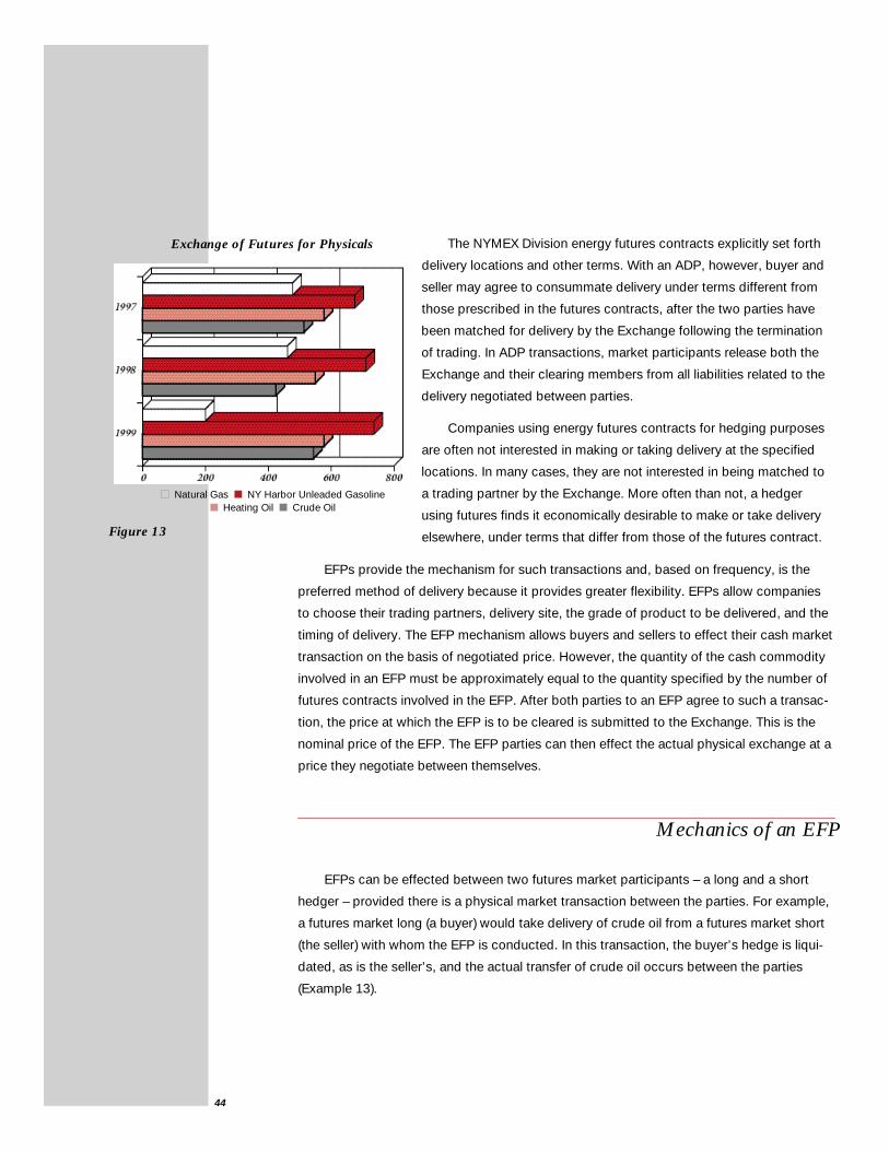
44
The NYMEX Division energy futures contracts explicitly set forth
delivery locations and other terms. With an ADP, however, buyer and
seller may agree to consummate delivery under terms different from
those prescribed in the futures contracts, after the two parties have
been matched for delivery by the Exchange following the termination
of trading. In ADP transactions, market participants release both the
Exchange and their clearing members from all liabilities related to the
delivery negotiated between parties.
Companies using energy futures contracts for hedging purposes
are often not interested in making or taking delivery at the specified
locations. In many cases, they are not interested in being matched to
a trading partner by the Exchange. More often than not, a hedger
using futures finds it economically desirable to make or take delivery
elsewhere, under terms that differ from those of the futures contract.
EFPs provide the mechanism for such transactions and, based on frequency, is the
preferred method of delivery because it provides greater flexibility. EFPs allow companies
to choose their trading partners, delivery site, the grade of product to be delivered, and the
timing of delivery. The EFP mechanism allows buyers and sellers to effect their cash market
transaction on the basis of negotiated price. However, the quantity of the cash commodity
involved in an EFP must be approximately equal to the quantity specified by the number of
futures contracts involved in the EFP. After both parties to an EFP agree to such a transac-
tion, the price at which the EFP is to be cleared is submitted to the Exchange. This is the
nominal price of the EFP. The EFP parties can then effect the actual physical exchange at a
price they negotiate between themselves.
Mechanics of an EFP
EFPs can be effected between two futures market participants – a long and a short
hedger – provided there is a physical market transaction between the parties. For example,
a futures market long (a buyer) would take delivery of crude oil from a futures market short
(the seller) with whom the EFP is conducted. In this transaction, the buyer’s hedge is liqui-
dated, as is the seller’s, and the actual transfer of crude oil occurs between the parties
(Example 13).
Exchange of Futures for Physicals
Figure 13
■ Natural Gas ■ NY Harbor Unleaded Gasoline■ Heating Oil ■ Crude Oil
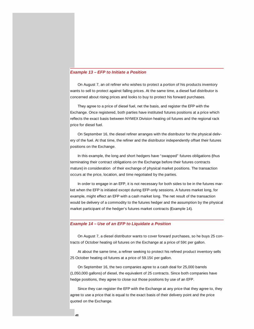
45
Example 13 – EFP to Initiate a Position
On August 7, an oil refiner who wishes to protect a portion of his products inventory
wants to sell to protect against falling prices. At the same time, a diesel fuel distributor is
concerned about rising prices and looks to buy to protect his forward purchases.
They agree to a price of diesel fuel, net the basis, and register the EFP with the
Exchange. Once registered, both parties have instituted futures positions at a price which
reflects the exact basis between NYMEX Division heating oil futures and the regional rack
price for diesel fuel.
On September 16, the diesel refiner arranges with the distributor for the physical deliv-
ery of the fuel. At that time, the refiner and the distributor independently offset their futures
positions on the Exchange.
In this example, the long and short hedgers have “swapped” futures obligations (thus
terminating their contract obligations on the Exchange before their futures contracts
mature) in consideration of their exchange of physical market positions. The transaction
occurs at the price, location, and time negotiated by the parties.
In order to engage in an EFP, it is not necessary for both sides to be in the futures mar-
ket when the EFP is initiated except during EFP-only sessions. A futures market long, for
example, might effect an EFP with a cash market long. The net result of the transaction
would be delivery of a commodity to the futures hedger and the assumption by the physical
market participant of the hedger’s futures market contracts (Example 14).
Example 14 – Use of an EFP to Liquidate a Position
On August 7, a diesel distributor wants to cover forward purchases, so he buys 25 con-
tracts of October heating oil futures on the Exchange at a price of 59¢ per gallon.
At about the same time, a refiner seeking to protect his refined product inventory sells
25 October heating oil futures at a price of 59.15¢ per gallon.
On September 16, the two companies agree to a cash deal for 25,000 barrels
(1,050,000 gallons) of diesel, the equivalent of 25 contracts. Since both companies have
hedge positions, they agree to close out those positions by use of an EFP.
Since they can register the EFP with the Exchange at any price that they agree to, they
agree to use a price that is equal to the exact basis of their delivery point and the price
quoted on the Exchange.
46
By using the EFP, the hedge was taken off using the exact basis. This avoided the pos-
sible market risk of covering the hedge in the open market at the Exchange where there is
no guarantee as to the price at which the hedge would be liquidated.
The above transaction is fairly straightforward. For example, a futures market long (a
cash market short) receives heating oil from a firm selling the commodity in the physical mar-
ket (a cash market long). The obligation of the futures market long to take delivery of heating
oil in New York Harbor is then ended. The firm selling the heating oil to the hedger would then
assume a new long futures position as of the date the EFP is posted at the Exchange.
The seller of heating oil then has three choices: (1) sell futures to liquidate its new
futures position; (2) let the contracts mature and take delivery of the heating oil in New York
Harbor; or (3) locate another firm willing to engage in an EFP.
Because EFPs might involve deliveries to points other than those specified in the con-
tracts, and/or different energy commodities, and/or different delivery periods, transaction
prices must be negotiated between parties to the EFPs. These negotiated prices could
reflect differentials based on quality, location, and timing, including transportation and qual-
ity differentials between the two products, and delivery points. In an EFP where gasoline is
delivered in Houston, negotiated prices might be a function of the location differential:
delivery in Houston instead of New York Harbor. Similarly, a delivery of jet fuel to Chicago
might be based on the product and location differentials: Chicago vs. New York Harbor and
jet fuel vs. heating oil.
The Exchange clearinghouse treats EFPs as trades for margining purposes. Once the
EFP is effected, margin funds can be released on the business day following the posting of
the EFP.
In EFPs involving a futures market hedger and a physical product market participant
that initially is not holding a futures position, the hedger’s margin funds are released on the
business day following the EFP posting. The physical market participant then becomes
responsible for maintaining the account established for margin funds until the hedge is liq-
uidated or delivery of the contracts is made.
EFPs can be negotiated at the time a particular energy futures contract trades or until
2 P.M. of the business day following the termination of trading in an expired contract for
crude oil, petroleum products, and electricity, and two hours after the termination of trading
in the natural gas contracts. After both parties to an EFP agree to such a transaction, the
Exchange must be notified of their intention to effect the EFP through the parties’ clearing
members.
The Exchange requires written documentation on EFPs and provides standardized
forms for this purpose. Information to be supplied includes:
47
■ The fact that an EFP transaction is being effected.
■ A statement that the EFP has resulted in a change in ownership of a
particular energy commodity.
■ The date the transaction occurred.
■ The type and quantity of the energy futures involved in the EFP transaction.
■ The price at which the futures transaction is to be cleared.
■ The names of the clearing members involved in the EFP.
The buyer’s and seller’s clearing members must satisfy the Exchange that the transac-
tion is a legitimate EFP. Evidence of a change in ownership of the cash commodity involved
in the EFP (or a commitment for such a change), as well as payment received by the firm
selling the product, must be made available to the Exchange and secured by the clearing
members representing the parties to the EFP upon specific request from the Exchange’s
compliance department.
Blind vs. Selective Hedge
The term “blind hedge” refers to the practice of not deviating from a fully planned
hedging strategy, with volumes, contracts, and entry and exit points established prior to the
execution of the hedge. In a selective hedge, the execution of the overall strategy can be
fine-tuned to better reflect ongoing cash market conditions. Thus, if a third case of continu-
ously increasing postings were assumed, it is unlikely that the producer would blindly stick
to his losing short hedges, rather than liquidate early to contain his future losses. A selec-
tive hedge, for example, might link the volume to be hedged to an ongoing assessment of
the cash-futures basis relationship and the perceived likelihood of a reduction in posted
prices.
Technical Analysis
The word “technical” is often used in connection with the action of prices in the futures
market. Often heard phrases are: the market declined because of a “technical reaction,” it
went up on a “technical rally,” the market is “technically weak” or “technically strong.”
Technical is used to mean a price movement based on a continuation of, or deviation from,
an observed price pattern.
48
The market price of a specific commodity is considered by technical traders to be the
most important determinant of the environment which will affect futures prices. Through the
use of the information revealed from charting daily futures prices, technicians attempt to
make accurate predictions regarding futures price behavior.
Charting Price Trend Lines
Charting is the practice of recording, in graph format, the market price movements of a
particular commodity over time with the objective of defining price levels at which com-
modities should be bought or sold. Daily price movements are plotted as high, low, and
closing prices to help the trader determine trends, resistance points at which prices should
not be easily exceeded, and support points below which prices should not easily fall. These
technical signals are used by traders to indicate when to buy or sell.
Trend lines are the simplest form of technical analysis. Connecting a series of high
points to draw a downtrend can give the trader his first set of clues to current market direc-
tion. Using lows and highs together, in either direction, will yield a price channel between
the two lines, indicating if and when a piece breakout beyond the channel may occur.
Moving averages represent a more complex way of identifying these underlying trends.
Technical traders always trade with the trend, never against it. While there will always
be moderate rallies in downtrends and moderate reactions in uptrends, countertrend move-
ment is seldom sustained.
A variety of patterns have been identified to help recognize changes in a trend. Chart
patterns have been variously described as “double tops,” (when the market rises but hits
resistance at a certain level, retreats, rises again, but still cannot breach the previous resis-
tance point, and falls back again); “double bottoms,” an inverse pattern that shows resis-
tance to a falling market; “head-and-shoulder formations,” again the same general pattern,
but with the resistance points being hit at succeedingly lower (or higher) levels; “triangular
flag patterns,” when the market consolidates sideways; and “price gaps,” when the low
price of one bar on a chart is higher than the high of the preceding bar (or inversely, the high
is lower than the low of the preceding bar, a price or price range where no trades take
place).
Other techniques and terms which are commonly used in technical analysis include:
■ Historical Volatility: Analysis of a commodity’s past price variability based on time
frame (for example, 20-day) and price interval.
49
■ Moving Average: Moving average (open, high, low, close, midpoint, average) to
follow the trend signal data fluctuations, and signal long and short positions.
■ Ratio: Despite large fluctuations in price, many commodities have price relation-
ships. By calculating and analyzing their ratio, overvalued and undervalued markets can be
found.
■ Rate of Change: Monitors and calculates the market’s rate of change relative to
previous trend intervals, as specified in the value input (also known as peaks and valleys).
■ Relative Strength Index (RSI): Study to measure the market’s strength and weak-
ness. A high RSI (>70) indicates an overbought or weakening market, and a low RSI (<30) an
oversold, bear market.
■ Stochastic Oscillator: A computer-generated overbought/oversold indicator
whose traditional interpretation is similar to that of the RSI. A high stochastic reading (>80)
indicates an overbought, or weakening, market and a low reading (<20) indicates an over-
sold market.
■ Support/Resistance/Reversal: Levels determined through technical analysis that
indicate trading support, resistance, or the reversal (inverse) of a market price in a specific
time frame.
Interested readers can familiarize themselves with the concepts of technical trading
through various books and periodicals on the subject.
Volume and Open Interest
Figures for volume and open interest are also important and widely used technical trad-
ing tools. Volume refers to the total number of trades in a particular commodity futures con-
tract on a given day. Increasing volume is generally considered an indication that the current
price trend is strong and likely to continue. Changes in average volume figures are seen as
indicating when major high or low points in a market are being approached. Technical
traders believe volume will increase rapidly as these points are approached.
Open interest refers to the number of long and short positions in a specific contract
which have not been liquidated or offset by an opposing purchase or sale by the same par-
ticipant. Increasing open interest figures are considered supportive of the underlying price
trend. That is, they may indicate market strength during periods of rising prices, or the sup-
port of a downward trend during periods of market weakness. Similarly, decreasing open

50
interest figures during rising price trends are seen to indicate a technical weakness in the
market – a possible dip or reversal based upon the liquidation of long open interest.
Open interest is also an indicator of commercial use of a futures contract.
The combination of volume and open interest figures, used in conjunction with a major
technical analysis system, can provide useful information that traders can factor into their
decision-making process. Parallel or inverse relationships between volume and open inter-
est can be analyzed to determine the degree of support which may exist for a specific
price trend.
51
OPTIONS
Options on futures offer additional flexibility in managing price risk. There are two
types of options, calls and puts. A call gives the holder, or buyer, of the option the right, but
not the obligation to buy the underlying futures contract at a specific price up to a certain
time. A put gives the holder the right, but not the obligation to sell the underlying futures
contract at a specific price up to a certain time. A call is purchased when the expectation is
for rising prices; a put is bought when the expectation is for neutral or falling prices.
The target price at which a buyer or seller purchases the right to buy or sell the options
contract is the exercise price or strike price. The buyer pays a premium, or the price of the
option, to the seller for the right to hold the option at that strike.
An options seller, or writer, incurs an obligation to perform should the option be exer-
cised by the purchaser. The writer of a call incurs an obligation to sell a futures contract and
the writer of a put has an obligation to buy a futures contract.
An option is a wasting asset. The premium declines as time passes. Depending upon
the movement of an option’s price, the buyer will choose one of three alternatives to termi-
nate an options position: Exercise the option; liquidate it by selling, or buying, it back on the
Exchange; or let it expire without value.
Options give hedgers the ability to protect themselves from adverse price moves while
participating in favorable price moves. If the options contract expires worthless, the only
cost is the premium. Many people think of buying options like buying insurance.
By using options alone, or in combination with futures contracts, strategies can be
devised to cover virtually any risk profile, time horizon, or cost consideration.
Options Rights and Obligations
Call
Buyer Has the right to buy a futures contract at a predetermined price on or
before a defined date.
Expectation: Rising prices
Seller Grants right to buyer, so has obligation to sell futures at predeter-
mined price at buyer’s discretion.
Expectation: Neutral or falling prices
Put
Buyer Has right to sell futures contract at a predetermined price on or before
a defined date.
Expectation: Falling prices
Seller Grants right to buyer, so has obligation to buy futures at a predeter-
mined price at buyer’s discretion.
Expectation: Neutral or rising prices

52
Determinants of an Options Premium
In return for the rights they are granted, options buyers pay options sellers a premium.
The four major factors affecting the price are:
■ Futures price relative to options strike price
■ Time remaining before options expiration
■ Volatility of underlying futures price
■ Interest rates
As in the futures market, options trading takes place in an open outcry auction market
on the floor of the Exchange or after-hours on NYMEX ACCESS®. While the value of futures
is tied to the underlying cash commodity through the delivery process, the value of an
option is related to the underlying futures contract through the ability to exercise the option.
Strike Price vs. Futures Price
Strike prices are listed in various increments, depending upon the contract.
The most important influence on an option’s price is the relationship between the
underlying futures price and the option’s strike price.
Depending upon futures prices relative to a given strike price, an option is said to be
at-the-money, in-the-money, or out-of-the-money. An option is at-the-money when the
strike price equals the price of the underlying futures contract.
An option is considered in-the-money when the price of the futures contract is above a
call’s strike price, or when the futures price is below a put’s strike price. An in-the-money
option has intrinsic value.
A call is out-of-the-money when the futures price is less than the options strike price.
For example, when the December electricity futures price is $18 per megawatt hour, the
December $19 call grants the holder of the options contract the right to buy a December
futures contract at $19 even though the market is at $18.
A put is out-of-the-money when the underlying futures price is higher than the put’s
strike price.
53
An option’s premium will usually equal or exceed whatever intrinsic value the option
has, if any. Intrinsic value is the amount by which an option is in-the-money.
Premium - Intrinsic Value = Time Value
Call Premium = Time Value + Intrinsic Value
Put Premium = Time Value + Intrinsic Value
Time Value
An options time value is the amount buyers are willing to pay for the option above its
intrinsic value. Out-of-the-money options carry all time premium since their intrinsic value is
zero, as do at-the-money options. As an option becomes deeply in- or out-of-the-money,
the time premium shrinks. As an options contract approaches expiration, or volatility
decreases, time value decreases. It is important to note that time value is equal for the
same strike and same expiration for both calls and puts.
The time value of an option shrinks as the expiration date approaches, all other factors
being equal. The reason is that there is less and less time for a major change in market
behavior, and a decreasing likelihood that the option will change in value.
Call/Put Parity
Options prices are linked to futures prices through the exercise feature. If at the call
option’s expiration, futures are trading at $17, a $16 call is worth $1, intrinsically the differ-
ence between the futures price and the strike price. This is because the holder of a $16 call
can exercise his option, receive a long futures position at $16, immediately turn around and
sell the futures contract for $17, and make $1. This is known as trading at parity. If the call
is only trading at, say, 30¢, then a trader can buy $16 calls, exercise them into long futures
at $16, sell them for $17 and make a risk-free 70¢, exclusive of transaction costs. Market
forces ensure that an opportunity like this cannot last long.
The option cannot have a negative value, so if the risk does not occur, that is, if futures
prices do not exceed the strike price, the option will be worth zero. There is no reason to
exercise an option to buy futures at $16 when the futures can be purchased at $13.
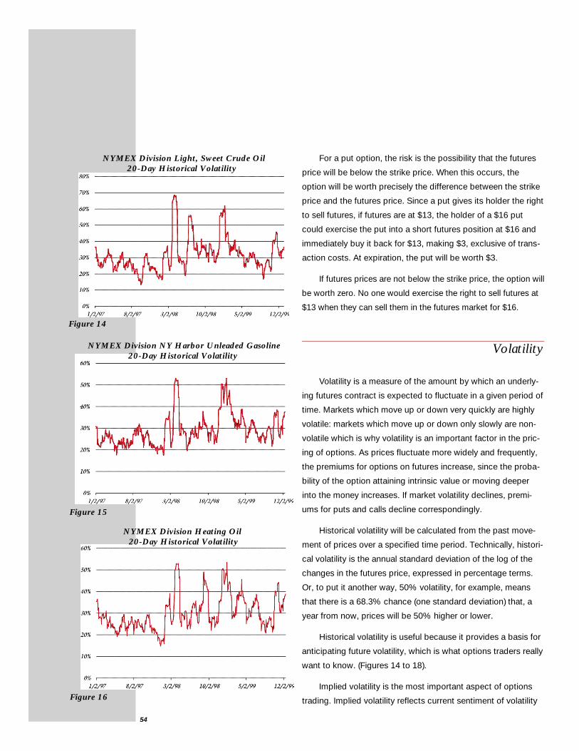
54
For a put option, the risk is the possibility that the futures
price will be below the strike price. When this occurs, the
option will be worth precisely the difference between the strike
price and the futures price. Since a put gives its holder the right
to sell futures, if futures are at $13, the holder of a $16 put
could exercise the put into a short futures position at $16 and
immediately buy it back for $13, making $3, exclusive of trans-
action costs. At expiration, the put will be worth $3.
If futures prices are not below the strike price, the option will
be worth zero. No one would exercise the right to sell futures at
$13 when they can sell them in the futures market for $16.
Volatility
Volatility is a measure of the amount by which an underly-
ing futures contract is expected to fluctuate in a given period of
time. Markets which move up or down very quickly are highly
volatile: markets which move up or down only slowly are non-
volatile which is why volatility is an important factor in the pric-
ing of options. As prices fluctuate more widely and frequently,
the premiums for options on futures increase, since the proba-
bility of the option attaining intrinsic value or moving deeper
into the money increases. If market volatility declines, premi-
ums for puts and calls decline correspondingly.
Historical volatility will be calculated from the past move-
ment of prices over a specified time period. Technically, histori-
cal volatility is the annual standard deviation of the log of the
changes in the futures price, expressed in percentage terms.
Or, to put it another way, 50% volatility, for example, means
that there is a 68.3% chance (one standard deviation) that, a
year from now, prices will be 50% higher or lower.
Historical volatility is useful because it provides a basis for
anticipating future volatility, which is what options traders really
want to know. (Figures 14 to 18).
Implied volatility is the most important aspect of options
trading. Implied volatility reflects current sentiment of volatility
NYMEX Division Light, Sweet Crude Oil
20-Day Historical Volatility
Figure 14
NYMEX Division NY Harbor Unleaded Gasoline
20-Day Historical Volatility
Figure 15
NYMEX Division Heating Oil
20-Day Historical Volatility
Figure 16
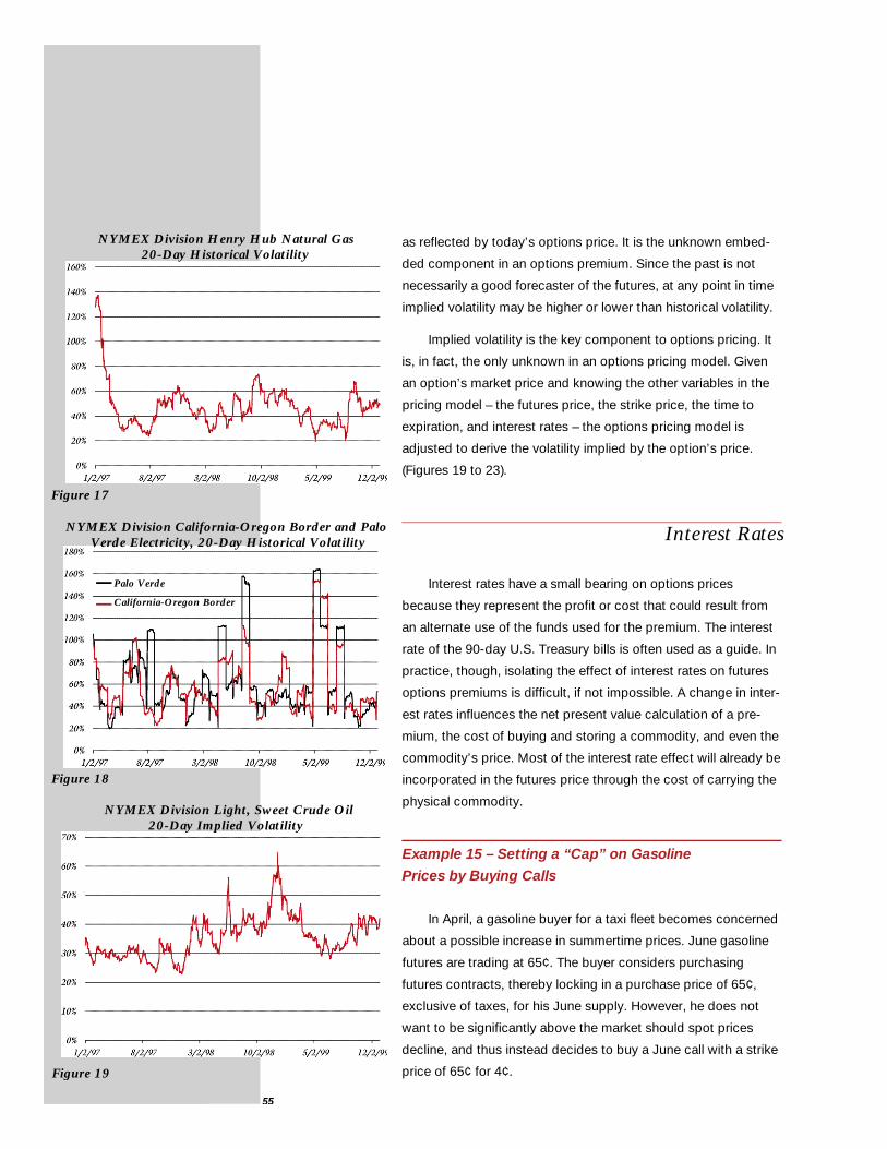
55
as reflected by today’s options price. It is the unknown embed-
ded component in an options premium. Since the past is not
necessarily a good forecaster of the futures, at any point in time
implied volatility may be higher or lower than historical volatility.
Implied volatility is the key component to options pricing. It
is, in fact, the only unknown in an options pricing model. Given
an option’s market price and knowing the other variables in the
pricing model – the futures price, the strike price, the time to
expiration, and interest rates – the options pricing model is
adjusted to derive the volatility implied by the option’s price.
(Figures 19 to 23).
Interest Rates
Interest rates have a small bearing on options prices
because they represent the profit or cost that could result from
an alternate use of the funds used for the premium. The interest
rate of the 90-day U.S. Treasury bills is often used as a guide. In
practice, though, isolating the effect of interest rates on futures
options premiums is difficult, if not impossible. A change in inter-
est rates influences the net present value calculation of a pre-
mium, the cost of buying and storing a commodity, and even the
commodity’s price. Most of the interest rate effect will already be
incorporated in the futures price through the cost of carrying the
physical commodity.
Example 15 – Setting a “Cap” on Gasoline
Prices by Buying Calls
In April, a gasoline buyer for a taxi fleet becomes concerned
about a possible increase in summertime prices. June gasoline
futures are trading at 65¢. The buyer considers purchasing
futures contracts, thereby locking in a purchase price of 65¢,
exclusive of taxes, for his June supply. However, he does not
want to be significantly above the market should spot prices
decline, and thus instead decides to buy a June call with a strike
price of 65¢ for 4¢.
NYMEX Division Henry Hub Natural Gas
20-Day Historical Volatility
Figure 17
NYMEX Division California-Oregon Border and Palo
Verde Electricity, 20-Day Historical Volatility
Figure 18
NYMEX Division Light, Sweet Crude Oil
20-Day Implied Volatility
Figure 19
Palo Verde
California-Oregon Border

56
On May 21, the gasoline buyer purchases spot fuel and liq-
uidates his options position. The chart below illustrates the
results if the price of gasoline has increased to 85¢ (Case A) or
if it has declined to 50¢ (Case B).
Case A Case B
Prices Increase Prices Decrease
May 21: Spot Price $0.85 $0.50
May 21: Futures Price $0.85 $0.50
Cash Market Cost of Gasoline $0.85 $0.50
Less: Gain/(Loss) on Options
Sales Price $0.20 $0
Purchase Price $0.04 $0.04
$0.16 ($0.04)
Effective Cost of Gasoline $0.69 $0.54
In Case A, the gasoline buyer pays 85¢ to his supplier for
fuel, but the financial offset provided by the 16¢ option profit
gives him an effective gasoline cost of 69¢.
The reason the buyer chose to pay this 4¢ becomes
apparent in Case B. The buyer pays his supplier 50¢. The 65¢
call – the right to buy futures at 65¢ – now has no market value
because futures are trading at 50¢. So there is a net loss of 4¢
– the options premium paid – on the options position, giving
the taxi fleet an effective gasoline cost of 54¢. This is 11¢ less
than if futures alone were used to obtain price protection.
Example 16 – Setting a “Floor” Against a
Gasoline Price Decline by Buying Puts
In April, a gasoline refiner is concerned that a cool rainy
summer will drive prices down. With June futures trading at 65¢
per gallon, the refiner considers selling futures to lock in that
price. He realizes, however, that if the weather is fair and con-
ducive to vacation traveling, prices could rise well above 65¢,
and he would like to be able to earn the higher revenue. He
decides, therefore, to use options instead of selling futures,
buying a June put with a strike price of 65¢ for 4¢.
NYMEX Division NY Harbor Unleaded Gasoline,
20-Day Implied Volatility
Figure 20
NYMEX Division Heating Oil,
20-Day Implied Volatility
Figure 21
NYMEX Division Henry Hub Natural Gas,
20-Day Implied Volatility
Figure 22
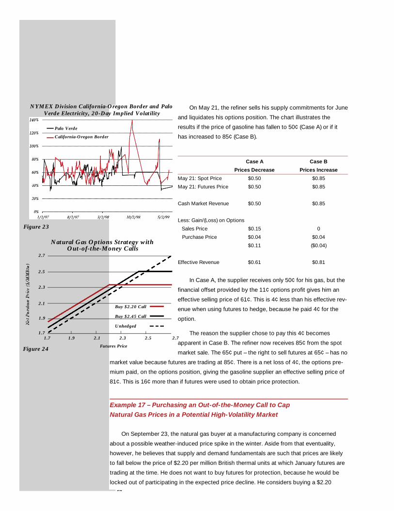
57
On May 21, the refiner sells his supply commitments for June
and liquidates his options position. The chart illustrates the
results if the price of gasoline has fallen to 50¢ (Case A) or if it
has increased to 85¢ (Case B).
Case A Case B
Prices Decrease Prices Increase
May 21: Spot Price $0.50 $0.85
May 21: Futures Price $0.50 $0.85
Cash Market Revenue $0.50 $0.85
Less: Gain/(Loss) on Options
Sales Price $0.15 0
Purchase Price $0.04 $0.04
$0.11 ($0.04)
Effective Revenue $0.61 $0.81
In Case A, the supplier receives only 50¢ for his gas, but the
financial offset provided by the 11¢ options profit gives him an
effective selling price of 61¢. This is 4¢ less than his effective rev-
enue when using futures to hedge, because he paid 4¢ for the
option.
The reason the supplier chose to pay this 4¢ becomes
apparent in Case B. The refiner now receives 85¢ from the spot
market sale. The 65¢ put – the right to sell futures at 65¢ – has no
market value because futures are trading at 85¢. There is a net loss of 4¢, the options pre-
mium paid, on the options position, giving the gasoline supplier an effective selling price of
81¢. This is 16¢ more than if futures were used to obtain price protection.
Example 17 – Purchasing an Out-of-the-Money Call to Cap
Natural Gas Prices in a Potential High-Volatility Market
On September 23, the natural gas buyer at a manufacturing company is concerned
about a possible weather-induced price spike in the winter. Aside from that eventuality,
however, he believes that supply and demand fundamentals are such that prices are likely
to fall below the price of $2.20 per million British thermal units at which January futures are
trading at the time. He does not want to buy futures for protection, because he would be
locked out of participating in the expected price decline. He considers buying a $2.20
NYMEX Division California-Oregon Border and Palo
Verde Electricity, 20-Day Implied Volatility
Figure 23
1.7 1.9 2.1 2.3 2.5 2.7
2.7
2.5
2.3
2.1
1.9
1.7
Futures Price
Natural Gas Options Strategy with Out-of-the-Money Calls
Figure 24
Buy $2.20 Call
Buy $2.45 Call
Unhedged
Palo Verde
California-Oregon Border
58
January at-the-money call for 15¢, but he knows that if prices do fall, his costs will be
higher by the 15¢ he pays for the call. After examining his budget, he decides he can afford
to pay approximately $2.50 for January gas. He then purchases a $2.45 call for 7¢.
The manufacturer has, in effect, decided to buy insurance against a severe price
increase. Believing the likelihood of a price increase is small, he is willing to absorb a signifi-
cant price move to reduce his insurance cost. The financial results of that decision are illus-
trated in Figure 24.
Had the gas buyer not hedged, his net purchase cost would be a 45-degree line. Had
he bought an at-the-money call, his purchase price would be higher by the amount of the
premium at prices up to the strike price. At a futures price of $2.35 (the strike plus the pre-
mium), he would break even. At higher futures prices, he would be cent-for-cent better off
having hedged.
By purchasing the out-of-the-money $2.45 call at prices up to $2.52 (the strike price
plus the seven-cent premium), the manufacturer will still pay more than if he had not
hedged. Compared to hedging with the at-the-money call, he is better off at futures prices
below $2.28. The breakeven point between two alternative strike calls is the lower strike
plus the difference in the premiums. In this example, $2.20 + ($0.15-$0.07)=$2.28. If he
believes prices are likely to be below $2.28 but he still wants protection against a dramatic
upward move, he is likely to choose to purchase the $2.45 call.
Example 18 – Hedging Against a Natural Gas Price Decline in a
Potential High-Volatility Market with Out-of-the-Money Puts
On September 23, a natural gas producer considers hedging against a warm winter. He
believes, however, that supply and demand fundamentals are such that even a normal win-
ter would not result in a sizable price increase. So he does not want to hedge with futures,
thereby locking in a January futures price of $2.20, nor does he want to spend 15¢ for an
at-the-money put. But knowing he will have cash flow problems if he has to sell January
gas for less than $1.85, he decides to buy a $1.95 put for 5¢.
The producer has decided to hedge against the markets becoming highly volatile by
purchasing an out-of-the-money put.
Had the producer purchased an at-the-money put, he would break even at $2.05 – the
$2.20 strike less the 15¢ premium. If futures prices are lower than that, he will be better off
having hedged with the $2.20 put.
With the $1.95 put, the producer’s breakeven price vis-a-vis being unhedged drops to
$1.90. But his breakeven level compared to the purchase of the $2.20 put is $2.10. The
59
breakeven point between the alternative strike puts is the higher strike less the difference in
the premiums. In this example, $2.20-($0.15-$0.05)=$2.10.
At higher futures prices, he will be better off with the out-of-the-money $1.95 put. If he
thinks prices are likely to go above $2.10, but he still wants downside protection, the $1.95
put is the logical choice.
Collars
Sometimes the cost of buying options can be more expensive than a company’s bal-
ance sheet allows. A collar strategy allows a hedger the opportunity to lower the cost of the
hedge, while creating a beneficial revenue stream.
A collar strategy involves the purchase (or sale) of a call, which is offset by the sale (or
purchase) of a put. The call and put both have out-of-the-money strike prices and expire in
the same month.
Example 19 – An Industrial Natural Gas Consumer Uses A Collar
To Hedge Prices At An Affordable Cost
With futures prices at $2.85, for example, an industrial natural gas consumer is
exposed to rising fuel costs and needs to set a cap. A cost of 19¢ for the $3.25 call is too
expensive for the company’s risk management committee. The company’s risk manager
decides to sell a $2.00 put for 19¢ and buy the call. A collar of $2.00 to $3.25 is now set.
The minimum he will pay for gas is $2.00, the maximum, $3.25.
CASE A CASE B CASE CFutures Futures Futures
Go to $1.50 Stay at $2.85 Rally to $4.00
Spot $1.50 $2.85 $4.00
Futures $1.50 $2.85 $4.00
Cash $1.50 $2.85 $4.00
Less Gain/(Loss) on Options
Offset of put ($0.50) 0 0(options expire without value)
Cost of call ($0.19) ($0.19) ($0.19)
Gain of premium on put $0.19 $0.19 $0.19
Offset of call 0 0 $0.75
Gain (loss) ($0.50) 0 $0.75
Effective cost of gas $2.00 $2.85 $3.25
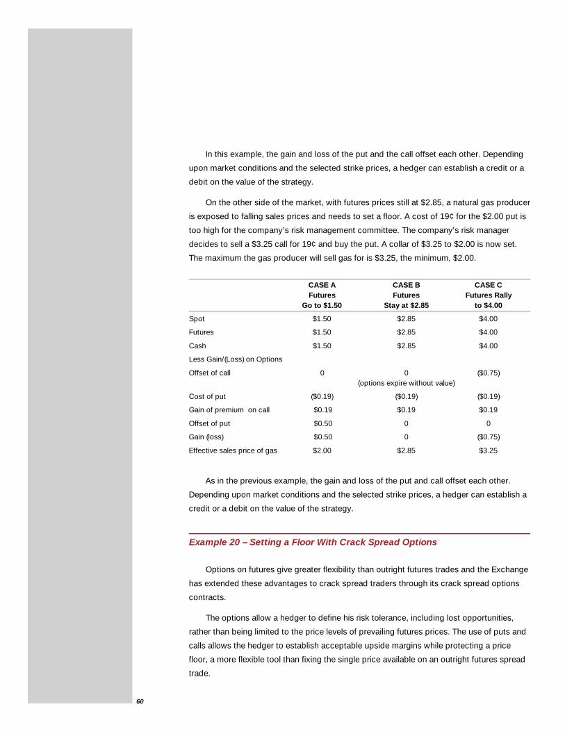
60
In this example, the gain and loss of the put and the call offset each other. Depending
upon market conditions and the selected strike prices, a hedger can establish a credit or a
debit on the value of the strategy.
On the other side of the market, with futures prices still at $2.85, a natural gas producer
is exposed to falling sales prices and needs to set a floor. A cost of 19¢ for the $2.00 put is
too high for the company’s risk management committee. The company’s risk manager
decides to sell a $3.25 call for 19¢ and buy the put. A collar of $3.25 to $2.00 is now set.
The maximum the gas producer will sell gas for is $3.25, the minimum, $2.00.
CASE A CASE B CASE CFutures Futures Futures Rally
Go to $1.50 Stay at $2.85 to $4.00
Spot $1.50 $2.85 $4.00
Futures $1.50 $2.85 $4.00
Cash $1.50 $2.85 $4.00
Less Gain/(Loss) on Options
Offset of call 0 0 ($0.75)(options expire without value)
Cost of put ($0.19) ($0.19) ($0.19)
Gain of premium on call $0.19 $0.19 $0.19
Offset of put $0.50 0 0
Gain (loss) $0.50 0 ($0.75)
Effective sales price of gas $2.00 $2.85 $3.25
As in the previous example, the gain and loss of the put and call offset each other.
Depending upon market conditions and the selected strike prices, a hedger can establish a
credit or a debit on the value of the strategy.
Example 20 – Setting a Floor With Crack Spread Options
Options on futures give greater flexibility than outright futures trades and the Exchange
has extended these advantages to crack spread traders through its crack spread options
contracts.
The options allow a hedger to define his risk tolerance, including lost opportunities,
rather than being limited to the price levels of prevailing futures prices. The use of puts and
calls allows the hedger to establish acceptable upside margins while protecting a price
floor, a more flexible tool than fixing the single price available on an outright futures spread
trade.
61
Assume the crack spread is trading at a reasonable $3 per barrel. A refiner may not be
ready to lock in that margin, hoping it will go higher, but he would want to protect against it
falling to less than $2.50. To accomplish this, the refiner would buy a $2.50 put while selling
a call at a strike price of $3.50. Such an arrangement allows the refiner to participate in a
favorable move to some extent above $3 while collecting premium income, and protects
him if the market falls below $2.50.
The refiner, however, gives up the opportunity to participate in a market rally above
$3.50 for the volume hedged. It is rare, though, that 100% of market exposure is hedged,
so the potential exists to benefit from the remaining unhedged position. In a case such as
the one presented here, the refiner would identify the percentage of the refinery margin he
wants to hedge at certain economics and will increase the percentage of hedged volume as
crack spread values increase.
A long crack spread put, such as the $2.50 put cited above, consists of being short the
product and long crude oil. Refiners as hedgers are natural crack spread longs as they are
continually buying crude and selling products. If crack spreads rise, or widen, only the pre-
mium is at risk. Meanwhile, the refiner is protected if refining margins should narrow.
Example 21 – Writing Call Options
Selling a crack spread options call is also a refiner’s strategy. It enhances returns on
refining margins as the premium income is used to offset the risk of declines in the product
market outpacing a decline in crude oil costs, and squeezing refining margins. A writer of
crack spread calls replicates a short product futures position and a long crude oil position.
Refiners are natural writers of calls. If the crack spread widens – that is, refining mar-
gins increase – a refiner could be at risk because the option could be exercised against
him. By selling a call, however, a refiner enhances his position by the amount of premium
he collects.
An integrated refiner with a substantial marketing network, however, is not as con-
cerned about finding a home for its products as in protecting its margin. Many refiners are
in a position where their marketing demand is greater than their refinery production. To
make up this deficit, they often must purchase products for resale. That places the com-
pany on both sides of the products market, as a buyer and a seller.
A company in that position also has to be concerned about the crack spread increas-
ing too rapidly for the volume of products that are purchased for resale from outside
sources.
62
In such a case, the refiner has to be careful not to sell the crack spread. Selling the
spread (buying the crude and selling the products) effectively locks in a margin, something
that is not desirable when depending on outside sources for supply, because if product
prices should suddenly strengthen, the purchaser-reseller would likely be at a great disad-
vantage. If he did sell the crack spread, however, he would have to liquidate his position
and buy it back when the products were transferred to the marketing group, an unneces-
sary step.
A company in that position would likely be better off buying a crack spread put, allow-
ing the hedger to protect his refining margin in the event prices fall.
That is a key advantage of the crack spread options. They allow a hedger to manage
both sides of the overall risk. A refiner in that position does not want the crack spread to go
down too far – he loses money on his production of refined products, nor does he want it to
go up too much – he loses on his purchase of products for resale.
Example 22: Creating a Fence with Crack Spread Options
The chart shows that the refiner’s purchase of a $2.50 crack spread put and his sale of
a $3.50 crack spread call assures the refiner that he will realize a margin of between $2.50
and $3.50 per barrel.
The strategy ensures that his margin will not fall below $2.50. If the crack spread drops
below $2.50, the long put position will make money, offsetting a loss in the physical market.
Should prices rally above $3.50, however, it is likely that the short call will be exercised.
Since the refiner also sells the physical product, however, the increased margin realized in
the cash market would offset his loss on the short options position.
In this example, the premium of both options is 20¢ per barrel, so the refiner’s cost of
the long put is $200 and his premium income on the short call is $200.
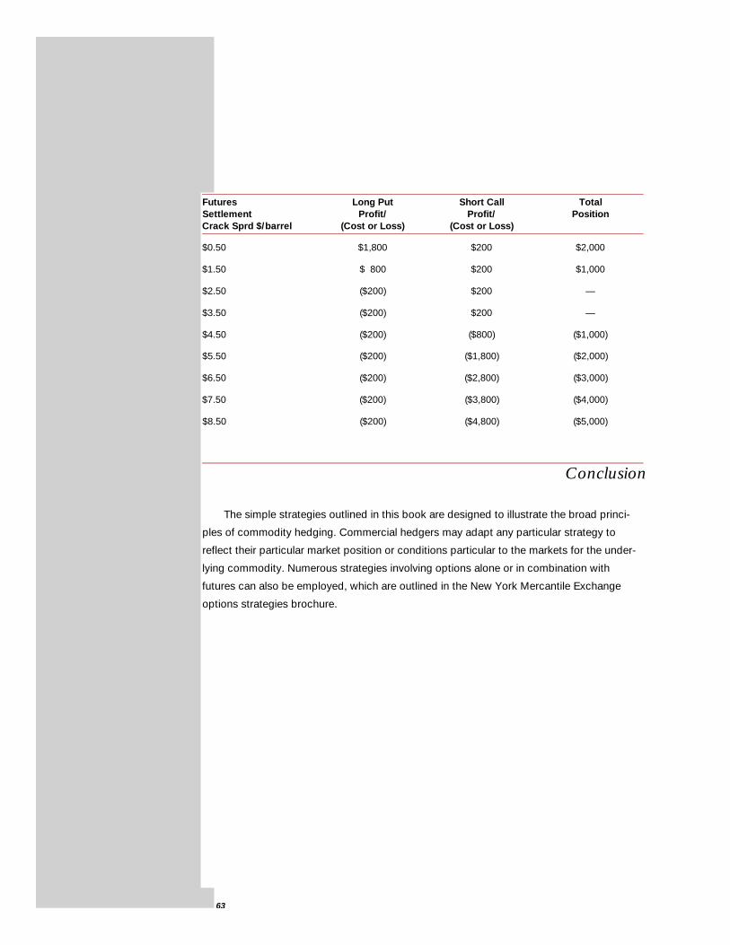
63
Futures Long Put Short Call TotalSettlement Profit/ Profit/ PositionCrack Sprd $/barrel (Cost or Loss) (Cost or Loss)
$0.50 $1,800 $200 $2,000
$1.50 $ 800 $200 $1,000
$2.50 ($200) $200 —
$3.50 ($200) $200 —
$4.50 ($200) ($800) ($1,000)
$5.50 ($200) ($1,800) ($2,000)
$6.50 ($200) ($2,800) ($3,000)
$7.50 ($200) ($3,800) ($4,000)
$8.50 ($200) ($4,800) ($5,000)
Conclusion
The simple strategies outlined in this book are designed to illustrate the broad princi-
ples of commodity hedging. Commercial hedgers may adapt any particular strategy to
reflect their particular market position or conditions particular to the markets for the under-
lying commodity. Numerous strategies involving options alone or in combination with
futures can also be employed, which are outlined in the New York Mercantile Exchange
options strategies brochure.
64
EXCHANGE INFORMATION
24-Hour Market Information Services
Telephone Access:
The Exchange’s public information office makes information available 24 hours a day
through Fastfacts, a state-of-the-art-phone system which puts you in touch with vital
Exchange information faster than ever.
NYMEX Division price and trading volume are available on Fastfacts with updates pro-
vided every five-minutes during the trading day by the Exchange’s mainframe computer.
New information is available within 30 minutes of real-time. Information pertaining to
Exchange holidays, delayed openings, and closings is also available.
NYMEX Division Fastfacts: (212) 301-4871
For a directory of access codes for all Exchange messages, contact the Exchange pub-
lications office at (212) 299-2777.
Internet Access:
The Exchange’s homepage, located at www.nymex.com, provides trading information,
including daily highs and lows, expiration dates, settlements, estimated volume, and
delayed prices for both futures and options; as well as contract specifications, Exchange
announcements, and holiday closings.
Price Histories
Price histories for all Exchange contracts are available on diskette, including light, sweet
crude oil; heating oil; unleaded gasoline; natural gas; electricity; propane; gold; silver; plat-
inum; palladium; copper; aluminum; options on the heating oil/crude oil and the New York
Harbor unleaded gasoline/ crude oil crack spread; and the FTSE Eurotop 100® and 300®
indexes. To order, contact the Exchange public information office at (212) 299-2318.
Quote Services
The Exchange’s daily futures and options price quotations are disseminated by a large
number of information service vendors. The Commodity Code Directory published by the
Exchange lists the principal information service vendors and the information retrieval codes

65
* FTSE®, FT-SE®, and Footsie® are trade and service marks of London Stock Exchange Ltd. and The Financial Times
Ltd. and are used by FTSE International Ltd. (“FTSE”) under license. “Eurotop” is a registered trademark of
Amsterdam Exchanges N.V. (“AEX”) or its subsidiaries and is used by FTSE under license. All copyright in the index val-
ues and constituent list vests in FTSE International Limited. The FTSE Eurotop 300® is calculated by FTSE
International Limited in conjunction with Amsterdam Exchanges and the Institute of Actuaries and the Faculty of
Actuaries in accordance with a standard set of ground rules. FTSE and AEX accept no liability in connection with the
trading of any contract on the Index.
for Exchange contracts. The Commodity Code Directory is also available on the
Exchange’s website.
Publications
The Exchange publishes magazines, a monthly newsletter, and brochures relating to the
energy and metals markets and the Exchange’s contracts. For a current list of publications,
to order publications, or for more information about the Exchange and its futures and
options contracts, write, call, or e-mail:
Publications Office
New York Mercantile Exchange
One North End Avenue, 15th Floor
World Financial Center
New York, NY 10282-1101
(212) 299-2777 Fax: (212) 301-4700
E-mail: [email protected]
The Exchange offers scheduled courses and on-site sessions about risk management.
For more information on educational programs, to learn more about using New York
Mercantile Exchange energy futures and options or other Exchange products, or to speak
to a marketing representative, please call (212) 299-2341, fax a request to (212) 301- 4570,
or e-mail at [email protected].
66
This brochure has been prepared for general information purposes only. Whilethe Exchange has made every effort to assure the accuracy of the information con-tained herein, any affirmation of fact in this brochure shall not create an express orimplied warranty that any example or description is correct. This brochure is madeavailable on the condition that errors or omissions shall not be made the basis forany claims, demands, or cause of action. 12/99