A Graphical Introduction to Special Relativity Based on a

Modern Approach to Minkowski Diagrams

B. Liu∗ and T. A. Perera†

Department of Physics, Illinois Wesleyan University,

P. O. Box 2900, Bloomington, IL 61702

(Dated: August 11, 2015)

Abstract

We present a comprehensive introduction to the kinematics of special relativity based on

Minkowski diagrams and provide a graphical alternative to each and every topic covered in a

standard introductory sequence. Compared to existing literature on the subject, our introduction

of Minkowski diagrams follows a more structured and contemporary approach. This work also

demonstrates new ways in which Minkowski diagrams can be used and draws several new insights

from the diagrams constructed. In this regard, the sections that stand out are: 1. the derivation

of Lorentz transformations (section III A through III D), 2. the discussion of spacetime (section

III F), 3. the derivation of velocity addition rules (section IV C), and 4. the discussion of relativis-

tic paradoxes (section V). Throughout the development, special attention has been placed on the

needs and strengths of current undergraduate audiences.

1

arX

iv:1

508.

0196

8v1

[ph

ysic

s.ed

-ph]

8 A

ug 2

015

I. Introduction

Most undergraduate physics students encounter Special Relativity and Quantum Me-

chanics in their second year through a course on Modern Physics. As these two topics do

not fit particularly well with the intuition and skills they develop in their first-year courses,

mathematical abstraction seems to be the path forward for many. If students are to gain

insights and develop intuition in these two subjects at an early stage, it is important to

make available to them several alternate routes of exploration. With regard to special rela-

tivity, students welcome the standard undergraduate introduction to Minkowski spacetime

diagrams, guessing that these diagrams will eventually be helpful for solving quantitative

problems. Unfortunately, this hope goes unrealized in most Modern Physics texts/courses

because the diagrammatic approach is not developed beyond the descriptive level. In our

experience, this does not stop students from attempting to adapt spacetime diagrams for

quantitative use, often unsuccessfully. What these students would truly appreciate is the

graphical construction introduced by Minkowski in his famous 1908 lecture on spacetime

diagrams,1 where the tilted and stretched x′-ct′ axes of a moving observer are overlaid on

the Cartesian x-ct grid of a stationary observer (for example, see Fig. 4). From now on,

we will use the term Minkowski diagram to refer to this quantitative graphical construction,

rather than the generic spacetime diagram (or x-ct plane) of a single observer.

The main purpose of this work is to showcase the multitude of ways in which Minkowski

diagrams can be used for instruction. In particular, we highlight several new ways of using

and interpreting Minkowski diagrams that we have developed. These together with well

established applications are presented here in one place, as a complete set of graphical

alternatives to all of the standard introductory lessons on the kinematics of special relativity.

Since standard pedagogy already makes use of spacetime diagrams in a qualitative sense,

extending their use for quantitative purposes is, we believe, a natural and expected step. It is

not our hope that the entire sequence laid out here will be adopted in full. However, continued

access to it will, we believe, benefit most students and instructors. We also hope that this

article will put Minkowski diagrams on the same footing as other (newer) diagrammatic

methods by presenting, in one place, a compilation of its uses, so that instructors may easily

gauge the relative strengths and weaknesses of different methods.

2

The Minkowski diagram has long been recognized as an effective quantitative tool in spe-

cial relativity.2–4 Then, why isn’t it used routinely in introductory treatments as a graphical

alternative or to reinforce standard algebraic methods? One reason implied in the literature,3

is the need for many geometrical constructs—triangles and invariant hyperbolae1,5—and

hence, “busy diagrams” in obtaining quantitative results. After a detailed survey of the

literature, another reason that stands out is the emergence of two other excellent graphical

techniques in the late 1950s to early 1960s, which was also the time when introductory treat-

ments of special relativity found their way into second-year undergraduate syllabuses. In

these two graphical constructions, named Loedel6,7 and Brehme8 diagrams, the two observers

are treated more symmetrically than in the Minkowski approach and, as a result, no stretch-

ing of x and ct axes are required for either observer. Hence, these diagrams were recognized

as superior, simpler, and more appropriate for introductory treatments. We contend that

the ultimate simplicity of Loedel and Brehme diagrams is achieved through a certain degree

of abstraction and cleverness, which may not be ideal for an intuition-building introduc-

tion to special relativity. For instance, identifying/drawing trajectories (worldlines) of the

two observers themselves on a Brehme diagram requires a few steps in reasoning,3,9 unlike

with Minkowski diagrams where these trajectories are obvious. Furthermore, Loedel and

Brehme diagrams cannot be used to derive special relativity from Einstein’s two postulates;

they are constructed by accepting the equality of the invariant interval between two inertial

observers.9 On the other hand, the Minkowski diagram can be constructed directly from the

postulates, and this is a valid method of deriving special relativity, as demonstrated in Max

Born’s text on relativity.10 In addition, the Loedel diagram and, therefore, the closely-related

Brehme diagram can be easily recognized as special applications of the Minkowski diagram.

Due to the above reasons or perhaps due to the perception that such an old technique

must have already reached its pedagogical potential, there does not exist a comprehensive

introductory treatment of special relativity, based on Minkowski diagrams, to the best of

our knowledge. Meanwhile detailed introductory sequences based on other graphical tech-

niques can easily be found in textbooks2,3 and pedagogy-oriented publications including this

journal.11 The closest parallels to these treatments, that utilize Minkowski diagrams, can be

found on the worldwide web,12 not in print journals. On the other hand, specific applica-

tions of Minkowski diagrams have appeared in the past literature13 as well as in more recent

3

journal articles.14 Unfortunately, authors of recent graphical treatments seem to be unaware

of the connection between their methods and the original work of Minkowski.

Over the past 2 years, we have assembled a complete and original lesson plan for intro-

ducing special relativity at the second-year level purely through Minkowski diagrams. The

complete cannon of introductory topics including the derivation of Lorentz transformations,

length contraction, time dilation, velocity addition, Doppler shift, and an exposition of well

know paradoxes are covered. In applying Minkowski diagrams to these topics, we have tried

to use modern arguments that would be most transparent to current second-year students,

given their usual preparation and experience at this stage. In particular, we have avoided

excessive use of geometrical constructs including invariant hyperbolae. Instead, we have pur-

sued a unique approach where where the x′-ct′ grid pattern of a moving observer is examined

using a mix of geometry and algebra. We have also tried to develop methods that are useful

for solving standard textbook problems in special relativity. These goals were achievable

mainly because the work was carried out as a student-faculty collaboration. The result of

this work, which we present here, is a streamlined introductory sequence made up of succinct

individual lessons that are often quite different from arguments/derivations we have seen in

the previous literature or on the web.

We start in section II with Galilean transformations and an introduction to the graphical

approach used here. In section III, using Einstein’s postulates and the previously developed

graphical ideas, work toward Lorentz transformations and the other kinematical results of

special relativity. In section IV, we demonstrate the usefulness of Minkowski diagrams in

deriving well know results and solving typical textbook problems. In section V, we demon-

strate the use of this method in unraveling several well known paradoxes of special relativity.

In this work, we will not cover the standard topics discussed in the context of generic space-

time diagrams, such as worldlines and light cones. Those topics can be introduced prior to

or in parallel with the development presented here.

II. Minkowski diagrams and Galilean transformations

We introduce Minkowski diagrams in the context of Galilean transformations so that

methods can be introduced independently from the surprises of relativity. Initially, spacetime

4

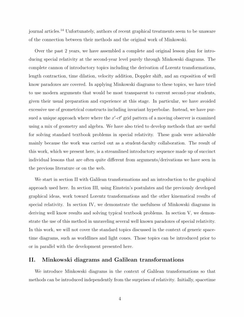
P

x x′

ct ct′

FIG. 1. The overlaid spacetime grids of observers A and B. The crosses represent clocks in B’s

frame separated by a unit length. The stars on the ct′ axis represent the ticks of the clock placed

at x′ = 0. The parallelogram in dark outline is the unit cell of B’s grid. The dashed lines indicate

how event P can be projected onto the x′-ct′ grid.

diagrams may be referred to as “time vs. position graphs,” as the unification of space and

time comes later. On these position-time graphs (e.g. Fig. 1), one spatial dimension (x) and

the ct axis will be displayed, following convention. Thus, the trajectories (worldlines) of light

pulses have slopes of ±1.

On Fig. 1, we first note the x-ct axes and square (dotted-line) grid of observer A, who is

stationary relative to the page. We regard A’s lines of constant x (vertical dotted lines) as

the worldlines of synchronized clocks spaced apart by unit length intervals along his x axis.

Along these worldlines, we mark a set of points corresponding to the ticks of each clock. The

lines of constant ct (horizontal dotted lines) are the lines connecting these clock ticks. Next,

we overlay on this graph the x′-ct′ grid of observer B, who is moving with speed v in the

+x direction of observer A. We do so by following the ticks and worldlines of equally-spaced

synchronized clocks in observer B’s reference frame. The positions of these clocks at t = 0

are marked by the crosses of Fig. 1. For convenience, the origins of the two grids intersect

5

at t = t′ = 0 and the spatial axes of the two coordinate systems are aligned with each other.

We can construct observer B’s position-time grid by adopting two “postulates” from day to

day experience: (1) the size of a unit ruler does not change due to one’s motion, and (2) all

the clocks of a moving observer remain synchronized with one another and with the clocks

of a stationary observer. It follows that the titled (light) solid lines of Fig. 1, with slope

c/v, are lines of constant x′ while the horizontal dotted lines serve as lines of constant ct′

as well. This type of diagram, where the position-time grids of both observers are overlaid,

is what we will refer to as a Minkowski diagram. In section III, we will replace the familiar

postulates (1) and (2) with Einstein’s postulates to arrive at the relativistically correct form

of the Minkowski diagram.

Now, given the x and ct coordinates of an event, such as event P of Fig. 1, one can project

it onto the x′-ct′ grid as indicated by the dashed lines. Using simple geometry and the fact

that there is no motion along the y and z axes, it is easy to show that

x′ = x− vt, y′ = y, z′ = z, t′ = t. (1)

Eqs. 1 are the Galilean transformations, which we have derived using postulates (1) and (2)

above. Before starting on relativity, it is important to point out some key results that follow

from Fig. 1. An object that moves with a constant velocity according to observer A would

be represented by a straight line in Fig. 1. This worldline would have a constant rise over

run (slope) on the x′-ct′ grid as well. Therefore, the object has a constant velocity according

to observer B as well. However, the x′ velocity will always differ from the x velocity by v,

the relative velocity between A and B.

III. Graphical derivation of the kinematics of special relativity

We begin with Einstein’s two postulates. A definition/explanation of inertial observers,

as those for whom the laws of physics assume their familiar and simple forms, should precede

this.

1. If an observer moves with constant velocity relative to an inertial observer, he/she is an

inertial observer as well.

2. All inertial observers will obtain/measure the same numerical value c for the speed of

6

light.

We note that under these two postulates, it is still possible for each inertial observer to

set up a system of synchronized clocks as before. Many introductory texts on relativity

describe in detail how a 3-d jungle gym of clocks can be synchronized, most often using light

signals, in a world where the above postulates are true.2 Thus, given that A is inertial, his

position-time grid can still be represented by the dotted lines of Fig. 1. Now, according

to postulate 1 above, B is also inertial, as he moves with constant velocity relative to A.

However, it is obvious that observer B’s coordinate grid can no longer be represented as in

Fig. 1 because, according to that representation, the speed of a light pulse moving in the

positive (negative) x direction of observer A would be c − v (c + v) for B. Our goal is to

find the correct representation of B’s grid. We will start by asking which aspects of Fig. 1

we should keep and which aspect we need to change.

A. Relaxation of Galilean assumptions

1. Observer B’s ct′ axis and other lines of constant x′ should continue to be straight lines

with slope c/v, because they are the worldlines of clocks that move along with observer B

at speed v relative to observer A.

2. Next, we ask if the stars along the ct′ axis of Fig. 1, which are the ticks of B’s clock

at unit time intervals, could be spaced differently than they are. It is easy to appreciate

that such a change would cause B’s speed of light measurements to yield values different

from c± v. Physically, we are asking whether we (and observer A) might observe B’s clocks

to be ticking at a different rate from A’s clocks due to B’s motion, even though all clocks

were manufactured identically. Although we will not answer this question definitively just

yet, let us keep the option to change the spacing between stars on the ct′ axis. We have

represented this freedom in Fig. 2. However, we require that the stars are equally spaced

along the (ct′) axis. Physically, this is equivalent to requiring that the relationship between

A’s clocks and B’s clocks depends solely on their relative motion and not on the specific

time on an observer’s clock or the absolute distance between observers.

3. Next, we turn our attention to the x′ axis. Our guiding principle here will be that all

observers identified as being inertial by A must also appear inertial to B. Thus, all straight

7

x

x′

ct ct′

FIG. 2. Here, we capture our present understanding of what B’s x′-ct′ coordinate system may

look like. The spacing between crosses (unit length markings), the spacing between stars (unit

time markings), and the angle of the x′ axis have been chosen arbitrarily here, as we have not

determined those parameters thus far. An important result is that B’s coordinate grid can be

completely characterized by the repeating unit-cell parallelogram highlighted here.

lines in A’s coordinate system should have a constant slope (rise over run) in B’s coordinates

as well. This constrains the x′ axis to be represented by a straight line and his unit length

markings along x′ (crosses) to be equally spaced. For the moment, we acknowledge the

possibility that the x′ axis may not be parallel to that of observer A and that the unit

length marks on it may be spaced differently from the unit length marks on A’s x axis. We

will elaborate on the physical significance of these potential differences later.

Fig. 2 encapsulates our present reasoning on what B’s position-time grid may look like.

An important result is that B’s position-time grid can be completely characterized by the

repeating parallelogram indicated in Fig. 2. Its sides represent B’s unit length and time

intervals. Therefore, we concentrate on this “unit cell” from now on.

8

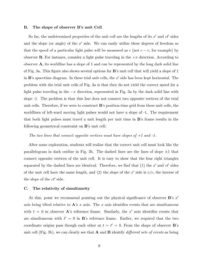
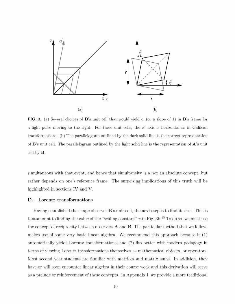
B. The shape of observer B’s unit Cell

So far, the undetermined properties of the unit cell are the lengths of its x′ and ct′ sides

and the slope (or angle) of the x′ side. We can easily utilize these degrees of freedom so

that the speed of a particular light pulse will be measured as c (not c − v, for example) by

observer B. For instance, consider a light pulse traveling in the +x direction. According to

observer A, its worldline has a slope of 1 and can be represented by the long dark solid line

of Fig. 3a. This figure also shows several options for B’s unit cell that will yield a slope of 1

in B’s spacetime diagram. In these trial unit cells, the x′ side has been kept horizontal. The

problem with the trial unit cells of Fig. 3a is that they do not yield the correct speed for a

light pulse traveling in the −x direction, represented in Fig. 3a by the dark solid line with

slope -1. The problem is that this line does not connect two opposite vertices of the trial

unit cells. Therefore, if we were to construct B’s position-time grid from these unit cells, the

worldlines of left-ward moving light pulses would not have a slope of -1. The requirement

that both light pulses must travel a unit length per unit time in B’s frame results in the

following geometrical constraint on B’s unit cell:

The two lines that connect opposite vertices must have slopes of +1 and -1.

After some exploration, students will realize that the correct unit cell must look like the

parallelogram in dark outline in Fig. 3b. The dashed lines are the lines of slope ±1 that

connect opposite vertices of the unit cell. It is easy to show that the four right triangles

separated by the dashed lines are identical. Therefore, we find that (1) the x′ and ct′ sides

of the unit cell have the same length, and (2) the slope of the x′ side is v/c, the inverse of

the slope of the ct′ side.

C. The relativity of simultaneity

At this, point we recommend pointing out the physical significance of observer B’s x′

axis being tilted relative to A’s x axis. The x axis identifies events that are simultaneous

with t = 0 in observer A’s reference frame. Similarly, the x′ axis identifies events that

are simultaneous with t′ = 0 in B’s reference frame. Earlier, we required that the two

coordinate origins pass though each other at t = t′ = 0. From the shape of observer B’s

unit cell (Fig. 3b), we can clearly see that A and B identify different sets of events as being

9

x x′

ct ct′

(a)

γ

γ

γ

v

cγ

v

cγ

(b)

FIG. 3. (a) Several choices of B’s unit cell that would yield c, (or a slope of 1) in B’s frame for

a light pulse moving to the right. For these unit cells, the x′ axis is horizontal as in Galilean

transformations. (b) The parallelogram outlined by the dark solid line is the correct representation

of B’s unit cell. The parallelogram outlined by the light solid line is the representation of A’s unit

cell by B.

simultaneous with that event, and hence that simultaneity is a not an absolute concept, but

rather depends on one’s reference frame. The surprising implications of this truth will be

highlighted in sections IV and V.

D. Lorentz transformations

Having established the shape observer B’s unit cell, the next step is to find its size. This is

tantamount to finding the value of the “scaling constant” γ in Fig. 3b.15 To do so, we must use

the concept of reciprocity between observers A and B. The particular method that we follow,

makes use of some very basic linear algebra. We recommend this approach because it (1)

automatically yields Lorentz transformations, and (2) fits better with modern pedagogy in

terms of viewing Lorentz transformations themselves as mathematical objects, or operators.

Most second year students are familiar with matrices and matrix sums. In addition, they

have or will soon encounter linear algebra in their course work and this derivation will serve

as a prelude or reinforcement of those concepts. In Appendix I, we provide a more traditional

10

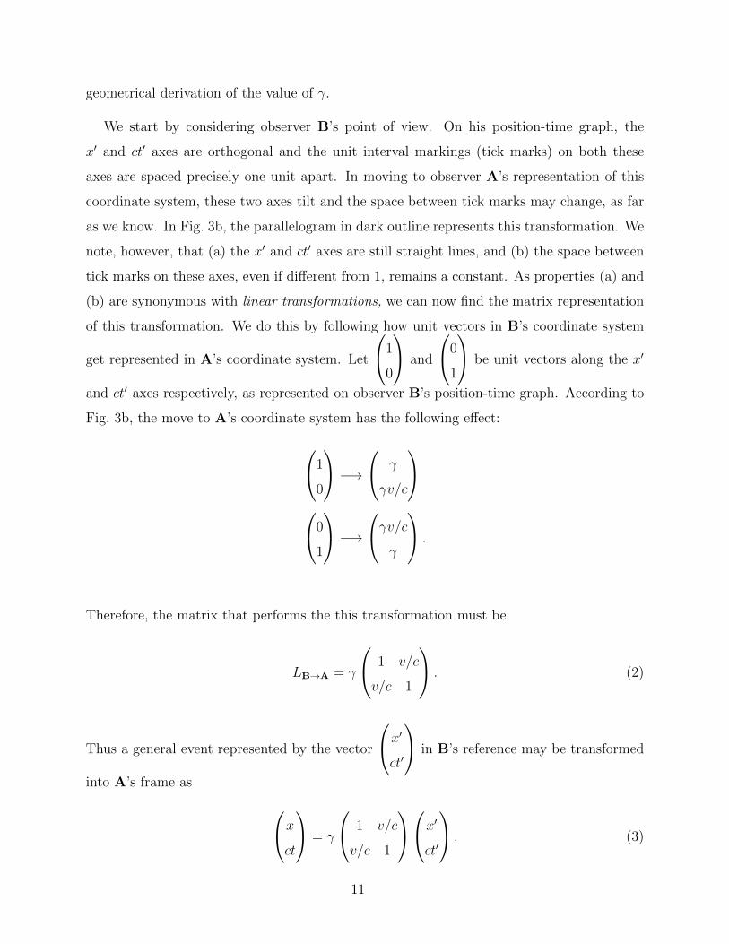
geometrical derivation of the value of γ.

We start by considering observer B’s point of view. On his position-time graph, the

x′ and ct′ axes are orthogonal and the unit interval markings (tick marks) on both these

axes are spaced precisely one unit apart. In moving to observer A’s representation of this

coordinate system, these two axes tilt and the space between tick marks may change, as far

as we know. In Fig. 3b, the parallelogram in dark outline represents this transformation. We

note, however, that (a) the x′ and ct′ axes are still straight lines, and (b) the space between

tick marks on these axes, even if different from 1, remains a constant. As properties (a) and

(b) are synonymous with linear transformations, we can now find the matrix representation

of this transformation. We do this by following how unit vectors in B’s coordinate system

get represented in A’s coordinate system. Let

1

0

and

0

1

be unit vectors along the x′

and ct′ axes respectively, as represented on observer B’s position-time graph. According to

Fig. 3b, the move to A’s coordinate system has the following effect:

1

0

−→ γ

γv/c

0

1

−→γv/c

γ

.

Therefore, the matrix that performs the this transformation must be

LB→A = γ

1 v/c

v/c 1

. (2)

Thus a general event represented by the vector

x′ct′

in B’s reference may be transformed

into A’s frame as xct

= γ

1 v/c

v/c 1

x′ct′

. (3)

11

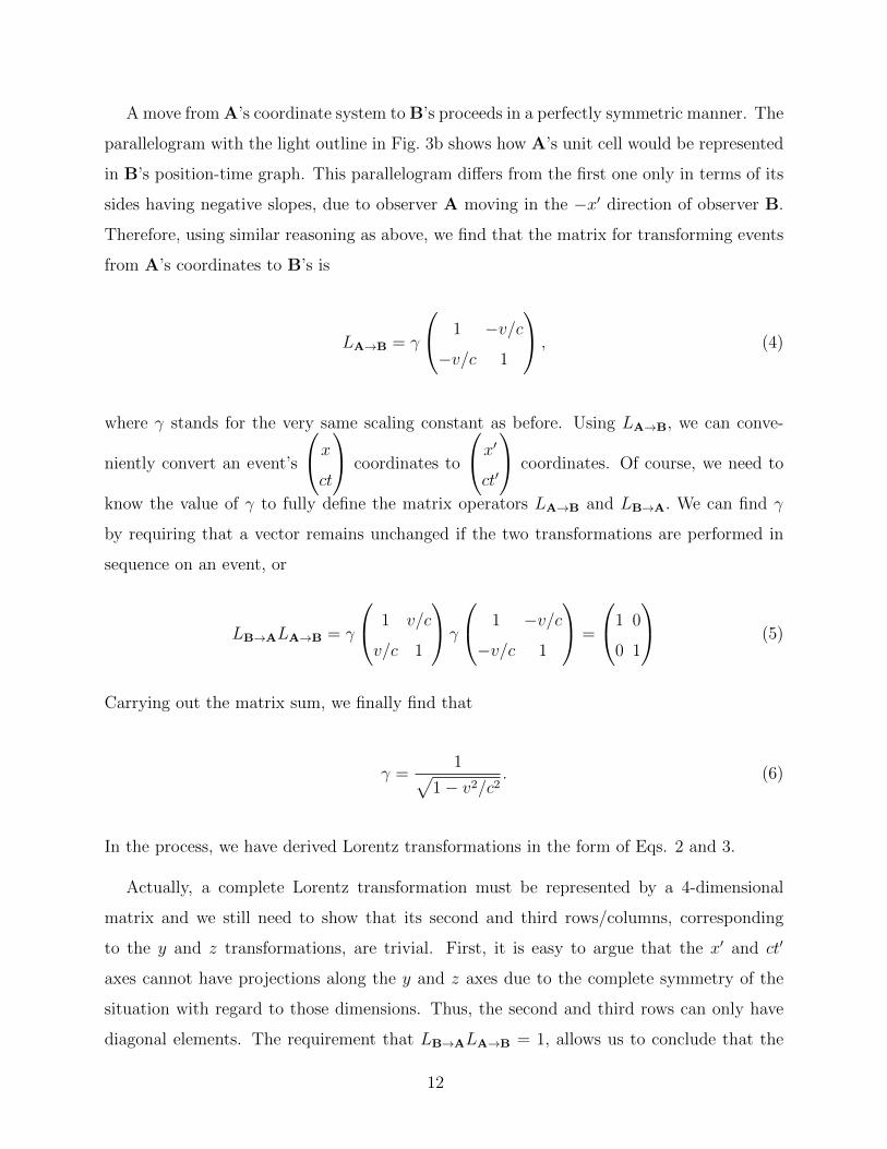
A move from A’s coordinate system to B’s proceeds in a perfectly symmetric manner. The

parallelogram with the light outline in Fig. 3b shows how A’s unit cell would be represented

in B’s position-time graph. This parallelogram differs from the first one only in terms of its

sides having negative slopes, due to observer A moving in the −x′ direction of observer B.

Therefore, using similar reasoning as above, we find that the matrix for transforming events

from A’s coordinates to B’s is

LA→B = γ

1 −v/c

−v/c 1

, (4)

where γ stands for the very same scaling constant as before. Using LA→B, we can conve-

niently convert an event’s

xct

coordinates to

x′ct′

coordinates. Of course, we need to

know the value of γ to fully define the matrix operators LA→B and LB→A. We can find γ

by requiring that a vector remains unchanged if the two transformations are performed in

sequence on an event, or

LB→ALA→B = γ

1 v/c

v/c 1

γ

1 −v/c

−v/c 1

=

1 0

0 1

(5)

Carrying out the matrix sum, we finally find that

γ =1√

1− v2/c2. (6)

In the process, we have derived Lorentz transformations in the form of Eqs. 2 and 3.

Actually, a complete Lorentz transformation must be represented by a 4-dimensional

matrix and we still need to show that its second and third rows/columns, corresponding

to the y and z transformations, are trivial. First, it is easy to argue that the x′ and ct′

axes cannot have projections along the y and z axes due to the complete symmetry of the

situation with regard to those dimensions. Thus, the second and third rows can only have

diagonal elements. The requirement that LB→ALA→B = 1, allows us to conclude that the

12

diagonal elements are 1. Thus, the complete Lorentz transformation will have the form

LA→B =

γ 0 0 −γv/c

0 1 0 0

0 0 1 0

−γv/c 0 0 γ

, (7)

Written out as individual equations, the final form of the Lorentz transformation is

x′ = γ(x− vt), y′ = y, z′ = z, t′ = γ(t− vx/c2). (8)

The opposite transformation (from B’s frame to A’s) looks identical except for a switch in

the signs preceding v.

E. Use and construction of relativistically correct Minkowski diagrams

Since the y and z transformations are trivial, the non-trivial content of Lorentz trans-

formations can be captured in the x-ct graph of Fig. 4. In it, we are now able to correctly

represent observer B’s spacetime diagram on top of observer A’s. In Fig. 4, the grid lines

parallel to the x and x′ axes should be viewed as lines of simultaneity for observers A and

B respectively. The lines parallel to the ct and ct′ axes represent fixed positions in their

respective reference frames.

In order to make quantitative use of diagrams such as Fig. 4, we need to know one more

geometric quantity: the size of unit intervals along the x′ and ct′ axes. These are the intervals

marked by stars and crosses on those axes. They obviously have unit length in observer B’s

own reference frame, but get stretched in the Lorentz transformation LB→A. In Fig. 3b, we

defined γ as the projection of the unit x′ interval onto the x axis and the unit ct′ interval

onto the ct axis. From this and the slopes of the x′ and ct′ axes in Fig. 4, we find that

length(x′ interval) = length(ct′ interval) = γ√

1 + v2/c2 (9)

Therefore, when converting a line-segment length along the x′ axis into and an actual

length that observer B would measure, we must divide by the factor γ√

1 + v2/c2. Similarly,

when converting a line-segment length along the ct′ axis into an actual time as judged by B,

13

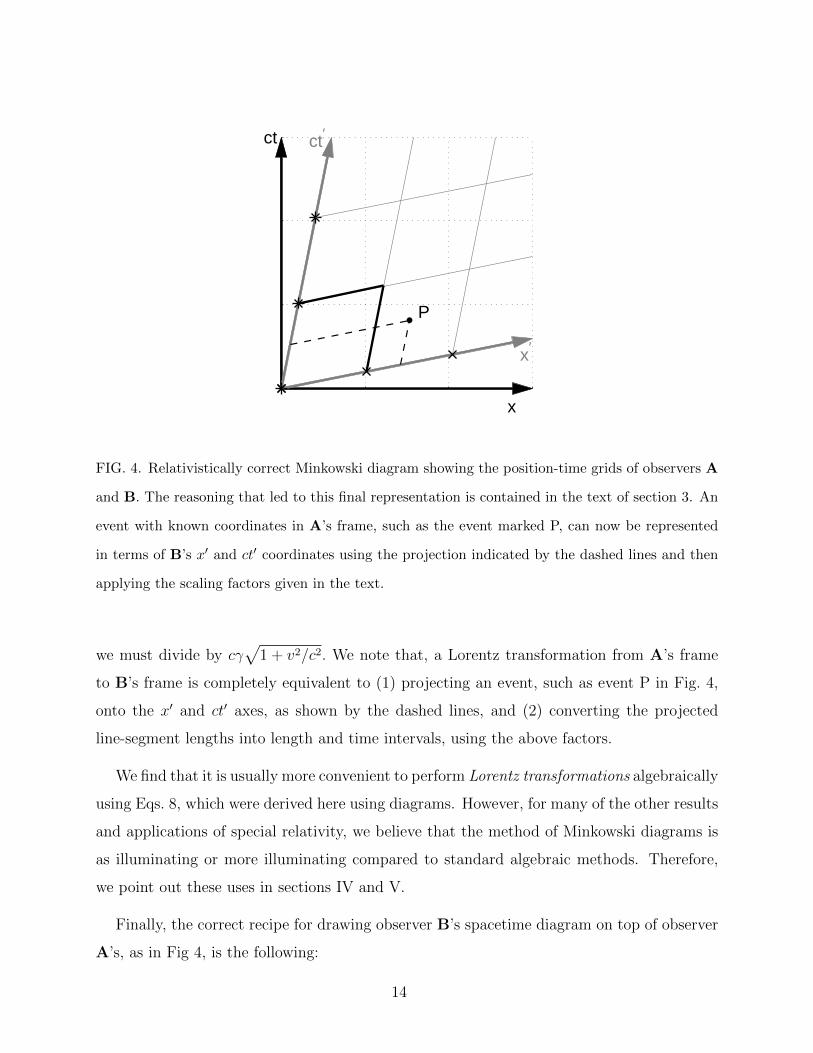
x

x′

ct ct′

P

FIG. 4. Relativistically correct Minkowski diagram showing the position-time grids of observers A

and B. The reasoning that led to this final representation is contained in the text of section 3. An

event with known coordinates in A’s frame, such as the event marked P, can now be represented

in terms of B’s x′ and ct′ coordinates using the projection indicated by the dashed lines and then

applying the scaling factors given in the text.

we must divide by cγ√

1 + v2/c2. We note that, a Lorentz transformation from A’s frame

to B’s frame is completely equivalent to (1) projecting an event, such as event P in Fig. 4,

onto the x′ and ct′ axes, as shown by the dashed lines, and (2) converting the projected

line-segment lengths into length and time intervals, using the above factors.

We find that it is usually more convenient to perform Lorentz transformations algebraically

using Eqs. 8, which were derived here using diagrams. However, for many of the other results

and applications of special relativity, we believe that the method of Minkowski diagrams is

as illuminating or more illuminating compared to standard algebraic methods. Therefore,

we point out these uses in sections IV and V.

Finally, the correct recipe for drawing observer B’s spacetime diagram on top of observer

A’s, as in Fig 4, is the following:

14

1. Draw the ct′ axis as a line of slope c/v that passes through the origin of the x-ct grid

of observer A.

2. Draw the x′ axis as a line of slope v/c that passes through the origin of the x-ct grid

of observer A. Thus, the angle between the x and x′ axes is the same as the angle

between the ct and ct′ axes.

3. Mark stars (clock ticks) along the ct′ axis and crosses (unit length intervals) on the x′

axis, separated by a distance γ√

1 + v2/c2.

In our case, the above steps are motivated by the entire development up to this point.

However, if one arrives at Lorentz transformations through a different route, these three

steps can be directly tied to the Lorentz transformation equations (Eqs. 8) as follows. Since

the ct′ axis is the x′ = 0 line, its equation on the x-ct plane can be found by setting to zero

the l.h.s. of the first equation in Eqs. 8. This motivates step 1 above. Similarly, step 2 can

be motivated by setting t′ = 0 in the last of Eqs. 8. Next, one can find the x′ = 1 line and

its intersection with the x′ axis, using Eqs. 8, to derive the size of unit length intervals on

the x′ axis (step 3). Unit ct′ intervals can be found in a similar way.

F. Spacetime and the invariant interval

In many introductory treatments, the idea of unifying space and time into one entity—

spacetime—is rationalized as follows: (1) unlike with Galilean transformations where time

is absolute, space and time are “mixed” thoroughly by Lorentz transformations; (2) there

exists a metric for spacetime that remains invariant between inertial observers. We believe

that, even at the introductory level, the concept of spacetime needs to be justified with more

quantitative substance than this. In particular, it should be pointed out that quantities of

spacetime are conserved by Lorentz transformations. What we mean here by a quantity or

amount of spacetime is the 4-dimensional hyper-volume occupied by a region of spacetime.

Algebraically, the above property is a consequence of proper Lorentz transformations

having unit determinant. However, at the introductory level this property can most easily

be demonstrated graphically. Because the y and z transformations are trivial, a 2-d diagram

such as Fig. 4 is sufficient for our purposes. In it, a 4-d hyper-volume of spacetime translates

to a 2-d area on the x-ct plane.

15

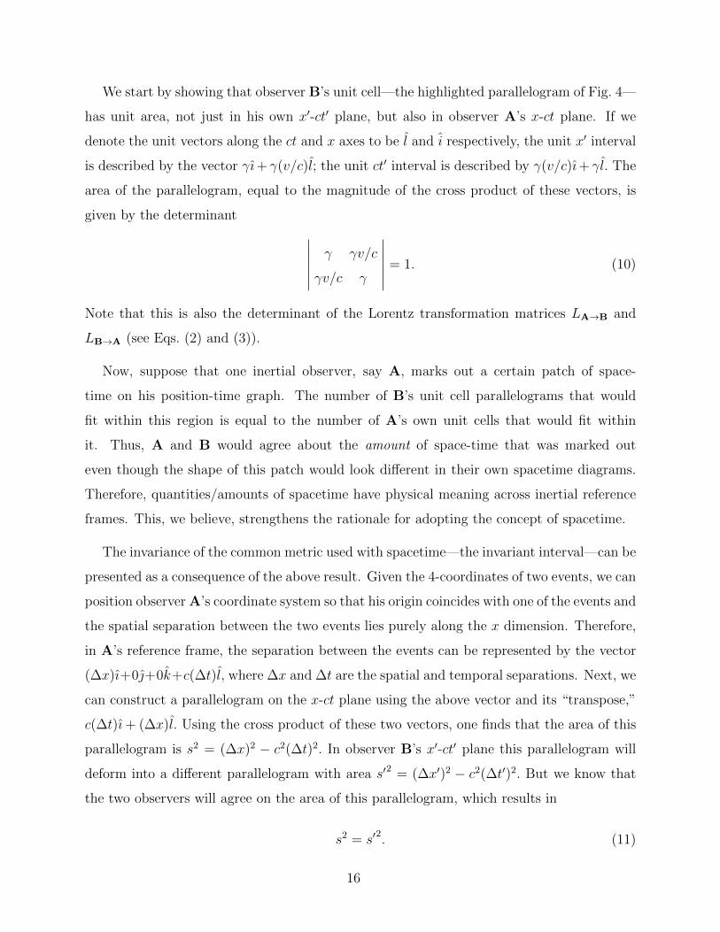
We start by showing that observer B’s unit cell—the highlighted parallelogram of Fig. 4—

has unit area, not just in his own x′-ct′ plane, but also in observer A’s x-ct plane. If we

denote the unit vectors along the ct and x axes to be l and i respectively, the unit x′ interval

is described by the vector γı+ γ(v/c)l; the unit ct′ interval is described by γ(v/c)ı+ γl. The

area of the parallelogram, equal to the magnitude of the cross product of these vectors, is

given by the determinant ∣∣∣∣∣∣ γ γv/c

γv/c γ

∣∣∣∣∣∣ = 1. (10)

Note that this is also the determinant of the Lorentz transformation matrices LA→B and

LB→A (see Eqs. (2) and (3)).

Now, suppose that one inertial observer, say A, marks out a certain patch of space-

time on his position-time graph. The number of B’s unit cell parallelograms that would

fit within this region is equal to the number of A’s own unit cells that would fit within

it. Thus, A and B would agree about the amount of space-time that was marked out

even though the shape of this patch would look different in their own spacetime diagrams.

Therefore, quantities/amounts of spacetime have physical meaning across inertial reference

frames. This, we believe, strengthens the rationale for adopting the concept of spacetime.

The invariance of the common metric used with spacetime—the invariant interval—can be

presented as a consequence of the above result. Given the 4-coordinates of two events, we can

position observer A’s coordinate system so that his origin coincides with one of the events and

the spatial separation between the two events lies purely along the x dimension. Therefore,

in A’s reference frame, the separation between the events can be represented by the vector

(∆x)ı+0+0k+c(∆t)l, where ∆x and ∆t are the spatial and temporal separations. Next, we

can construct a parallelogram on the x-ct plane using the above vector and its “transpose,”

c(∆t)ı+ (∆x)l. Using the cross product of these two vectors, one finds that the area of this

parallelogram is s2 = (∆x)2 − c2(∆t)2. In observer B’s x′-ct′ plane this parallelogram will

deform into a different parallelogram with area s′2 = (∆x′)2 − c2(∆t′)2. But we know that

the two observers will agree on the area of this parallelogram, which results in

s2 = s′2. (11)

16

x

x′

ct ct′

M

L

C

O

FIG. 5. The x-ct frame belongs to the ground observer while the x′-ct′ frame belongs to the pilot

(see text). OL represents the airstrip. The dashed line is the worldline of one end of the airstrip.

IV. Results and applications

The method of Minkowski diagrams is very useful for understanding the standard set of

“results” that arises from special relativity. These include time dilation, length contraction,

velocity addition, and the relativistic Doppler effect. Most textbook problems on special

relativity deal with these results. We stress that our methods are equally well suited for

introducing these topics as well as for working problems related to them.

A. Time dilation

With the above point in mind, we will discuss time dilation and length contraction in

terms of a problem that is typical of sophomore-level textbooks: An observer on the ground

sees an airplane traveling at speed v flying parallel to an airstrip of length l on the ground.

Therefore, she finds that the airplane traverses the length of the airstrip in time l/v. (a)

According to the pilot of the airplane, how much time does the airplane take to traverse the

length of the airstrip?

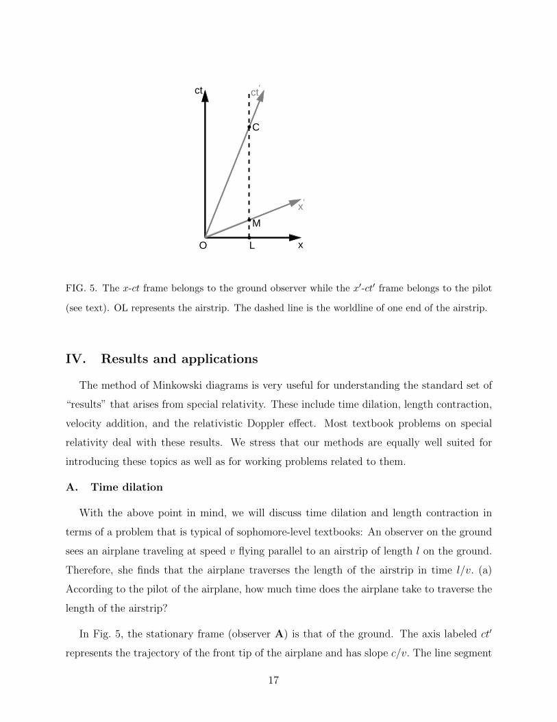
In Fig. 5, the stationary frame (observer A) is that of the ground. The axis labeled ct′

represents the trajectory of the front tip of the airplane and has slope c/v. The line segment

17

OL represents the airstrip and has length l. The worldline of the far end of the airstrip

(marked L) is represented by the vertical dashed line. The front tip of the airplane just

reaching the far end of the airstrip is represented by event C. The time interval of interest is

the time recorded for event C in the two reference frames. In the ground frame, c∆t is the

length of LC, which can be computed from the length of OL (l) and the slope of the ct′ axis

(c/v). We find that ∆t = l/v, as stated in the problem. The time of event C according to

the pilot (observer B) is directly related to the length of line segment OC, which is found to

be (cl/v)√

1 + v2/c2 from the Pythagorean theorem. As noted in section III E, this length

must be divided by cγ√

1 + v2/c2 in order to convert it to ∆t′. Thus, the time measured by

the pilot ∆t′ is different from ∆t = l/v; it is (l/v)/γ.

Students often have difficulty deciding if a given time interval is a proper time or not.

This is because they cannot visualize events such as O and C—the front tip of the airplane

intersecting the beginning and then the end of the airstrip—occuring at the same position

in one observer’s reference frame. Fig. 5 explicitly illustrates that OC is a proper time in

the pilot’s frame, as it lies on the ct′ axis (x′ = 0). Given the generality of the derivation, it

will also be clear that “improper” time intervals are always dilated by the factor γ relative

to proper time intervals.

B. Length contraction

The natural continuation of the above problem is: (b) Does the pilot of the airplane

measure a different length for the airstrip, and if so, what is that length?

Fig. 5 offers a good opportunity to stress what is meant by length. It is the instantaneous

distance between the end points of an object. In other words, it is the size of an object

measured along a line of simultaneity. For example, the unit length intervals along the x′

axis (marked with x’s in Fig. 4) are lengths for observer B, while OL in Fig. 5 represents a

length for observer A. Thus, the length of the airstrip as measured by the pilot is represented

by the line segment OM. From the slope of the x′ axis (v/c) and the Pythagorean theorem,

the length of OM is found to be l√

1 + v2/c2. As found in section III E, this must be divided

by γ√

1 + v2/c2 to yield a distance as measured by the pilot. Thus, the pilot measures the

airstrip to have length l/γ. Given the generality of this derivation, it is clear that the length

of an object is largest in its own rest frame; it is smaller by a factor of γ when measured

18

x

x′

ct ct′

projectileSP

T

FIG. 6. Event T represents observer B’s clock registering 1 unit of time. The tilted line (parallel to

the x′ axis) that goes through T is B’s unit-time line of simultaneity. It intersects the projectile’s

worldline at point P.

from a different frame.

C. Velocity addition

The question addressed here is: if a projectile moves with constant velocity U = Uxı +

Uy + Uzk in observer A’s reference frame, what is its velocity U′ = U ′xı+ U ′y + U ′zk in B’s

reference frame? A projection of this situation along the x direction is shown in Fig. 6. One

way for B to establish the projectile’s velocity is to measure the x′, y′, and z′ coordinates of

the projectile when exactly 1 time unit has elapsed on his own clock.

In Fig. 6, event T indicates B’s clock registering 1 unit of time. We know that events

simultaneous with this time are identified by the light solid line parallel to the x′ axis.

From the section on time dilation above (section IV A), we know that this line intersects

the ct axis at c(1/γ). Therefore, the expression for observer B’s unit-time simultaneity line

19

is ct = (v/c)x + c/γ. The projectile’s motion is described by the expression ct = (c/Ux)x.

Therefore, by setting these two equal, the coordinates of the event marked P are found to

be

xP =Ux

γ(1− Uxv/c2)(12)

tP =1

γ(1− Uxv/c2). (13)

Now, using Eq. 13, we can easily write down yP and zP, the y and z coordinates of the

projectile at time tP. Since the Lorentz transformation for y and z are trivial (see Eq. 8), we

find that

U ′y = y′P = yP = UytP =Uy

γ(1− Uxv/c2)(14)

U ′z = z′P = zP = UztP =Uz

γ(1− Uxv/c2). (15)

A common problem with relativistic velocity addition is the difficulty in intuiting why Ux

appears in the expressions for U ′y and U ′z, especially since the Lorentz transformations for

y and z and trivial. Fig. 6 is very useful in this regard. The critical step is to understand

the physical significance of event P. It represents the coordinates of the projectile, as judged

by observer B, exactly when his clock registers 1. Therefore, t′P = 1. However, tP clearly

depends on the slope of the projectile’s trajectory on the x-ct plane, and hence on Ux. It is

through tP that Ux finds its way into the expressions for U ′y and U ′z.

Next, we need to find U ′x. This is equal to x′P, which is represented by line segment TP in

Fig. 6. Knowing the equations for all the lines involved, it is possible to obtain the length of

TP algebraically. On the other hand, we can make quick progress by letting TP represent

a ruler in B’s reference frame. Note that the line segment SP then represents the length of

this ruler as determined by A.16 But

x′Pγ

= length(SP) = (Ux − v)tP, (16)

where the first equality follows from Lorentz-contraction and the second equality is simply

obtained from the relative speeds of the projectile and observer B. Substituting tP from

20

x

ct ct′

P1

P2

O

EtE

R

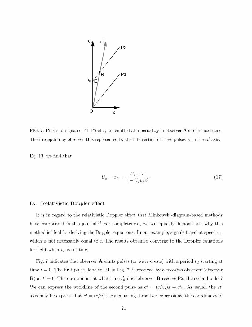
FIG. 7. Pulses, designated P1, P2 etc., are emitted at a period tE in observer A’s reference frame.

Their reception by observer B is represented by the intersection of these pulses with the ct′ axis.

Eq. 13, we find that

U ′x = x′P =Ux − v

1− Uxv/c2. (17)

D. Relativistic Doppler effect

It is in regard to the relativistic Doppler effect that Minkowski-diagram-based methods

have reappeared in this journal.14 For completeness, we will quickly demonstrate why this

method is ideal for deriving the Doppler equations. In our example, signals travel at speed vs,

which is not necessarily equal to c. The results obtained converge to the Doppler equations

for light when vs is set to c.

Fig. 7 indicates that observer A emits pulses (or wave crests) with a period tE starting at

time t = 0. The first pulse, labeled P1 in Fig. 7, is received by a receding observer (observer

B) at t′ = 0. The question is: at what time t′R does observer B receive P2, the second pulse?

We can express the worldline of the second pulse as ct = (c/vs)x + ctE. As usual, the ct′

axis may be expressed as ct = (c/v)x. By equating these two expressions, the coordinates of

21

event R (the reception of P2 by observer B) are found to be

xR =tE

1/v − 1/vs(18)

tR =tE

1− v/vs. (19)

Thus,

length(OR) =√c2t2R + x2R =

ctE1− v/vs

√1 + v2/c2. (20)

As discussed in section III E, length(OR) must be divided to cγ√

1 + v2/c2 to obtain t′R.

Thus, according to B, the time of reception of the second pulse

t′R =tE

γ(1− v/vs). (21)

So, the Doppler shift in frequency may be written as

f ′

f=tEt′R

= γ(1− v/vs). (22)

The case of approaching emitter and receiver may be treated in a very similar way after

extending Fig. 7 into the lower left quadrant where both x and ct are negative.

E. Other textbook problems

There is a class of textbook problems that calls for Lorentz transformations from one

reference frame to another. As mentioned in section III E, an event with known coordinates

in observer A’s reference frame can be projected onto observer B’s reference frame using

lines parallel to the x′ and ct′ axes. Thereafter, it is possible to find the x′ and ct′ values of

the event using purely geometry. However, we find that geometrical solutions turn out to be

as lengthy as the derivation of the Lorentz transformation. Therefore, we recommend using

Eqs. 8 for these problems, which were derived here using Minkowski diagrams.

In another class of problems, the 4-coordinates of two spatially and temporally separated

events are provided. Students are asked whether these two events can occur at the same

position in some observer’s reference frame and, if so, what the velocity of that observer

22

needs to be. Alternately, they are asked if the two events can be simultaneous for some

observer and, if so, what the velocity of the that observer needs to be. These problems

can be solved very easily using Minkowski diagrams and, in our experience, most relativity

instructors/texts do recommend spacetime diagrams for solving problems of this sort.

V. Paradoxes

The major theme that links the famous relativistic paradoxes is the relativity of simul-

taneity. The graphical methods developed here are especially helpful for visualizing the

latter and, therefore, for unraveling paradoxes. We will briefly describe how four well known

paradoxes can easily be visualized using the methods developed here.

A. The Andromeda paradox

In the following, we will refer to an observer’s lines of simultaneity as his/her “time-

frames.” From Minkowski diagrams, it is clear that even if observer B moves at a walking

pace relative to A, his time-frames are very slightly tilted relative to A’s time-frames. Ac-

cording to Fig. 4, events in the positive x direction, that are in B’s present time-frame are in

a future time-frame of observer A. Events in B’s present time-frame that are in the negative

x direction are in the past of observer A. Even when v (the relative velocity between A and

B) is very small, a difference in the time assigned to a remote event by A and B can be

quite large when the event is located very far away. For instance, suppose that intelligent

beings within the Andromeda galaxy have just now learned of the existence of humans on

earth. Now, by starting to walk in the direction of the Andromeda galaxy you will be able

to “dial in” to your time-frame a later date on the Andromedan’s calendar. Perhaps by that

date, after careful consideration, they have already launched a fleet of spaceships to conquer

the earth.

It is important to stress that this time-frame jump is a non-local (or remote) effect and

that, for instance, we cannot use it to influence the eventual actions of the Andromedan fleet.

However, as we will see in the context of the next paradox, the ability to dial in various dates

on a remote calendar into one’s time-frame can lead to interesting local effects as well.

23

B. The twin paradox

In this well known paradox, one twin stays on the earth while the other races to a distant

point in space at a significant fraction of c, quickly turns around, and returns to earth at

the same high speed. When they reunite, the earth-bound twin has aged more than the

astronaut twin. The apparent paradox is that the motion of the astronaut twin relative to

the earth-bound twin is exactly the same as the motion of the earth-bound twin relative to

the astronaut twin. Therefore, how can there be an asymmetry in their aging?

In most textbooks, it is explained that the simple time dilation calculation (dividing by

γ) is only applicable from an inertial, or non-accelerating, frame. Thus, we can employ the

simple calculation from the reference frame of the earth-bound twin but not the astronaut.

Therefore, the answer obtained this way by the earth-bound twin—that the astronaut twin

ages less—must be correct. To strengthen this argument, many authors use spacetime di-

agrams and follow the transmission and reception of light signals issued by the two twins.

These diagrams are very good at dispelling any doubts that the astronaut twin ages less.

However, these approaches fall short of pinpointing, as the explicit cause of unequal aging,

the intense acceleration of the astronaut twin during the turn-around. With Minkowski di-

agrams, we can directly visualize how one twin perceives the passage of time of the other

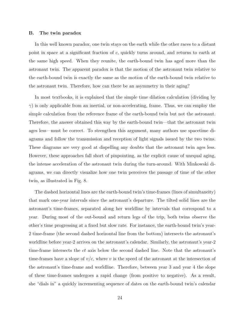
twin, as illustrated in Fig. 8.

The dashed horizontal lines are the earth-bound twin’s time-frames (lines of simultaneity)

that mark one-year intervals since the astronaut’s departure. The tilted solid lines are the

astronaut’s time-frames, separated along her worldline by intervals that correspond to a

year. During most of the out-bound and return legs of the trip, both twins observe the

other’s time progressing at a fixed but slow rate. For instance, the earth-bound twin’s year-

2 time-frame (the second dashed horizontal line from the bottom) intersects the astronaut’s

worldline before year-2 arrives on the astronaut’s calendar. Similarly, the astronaut’s year-2

time-frame intersects the ct axis below the second dashed line. Note that the astronaut’s

time-frames have a slope of v/c, where v is the speed of the astronaut at the intersection of

the astronaut’s time-frame and worldline. Therefore, between year 3 and year 4 the slope

of these time-frames undergoes a rapid change (from positive to negative). As a result,

she “dials in” a quickly incrementing sequence of dates on the earth-bound twin’s calendar

24

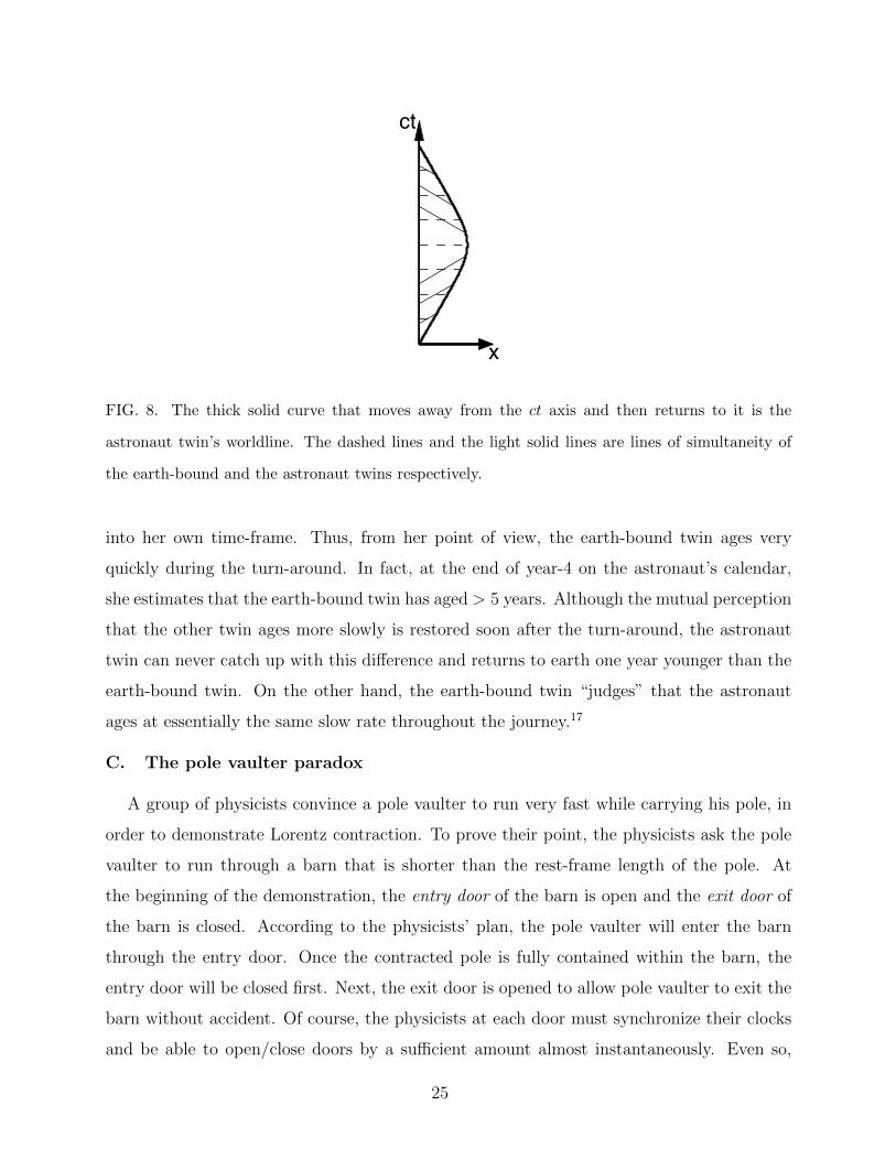
x

ct

FIG. 8. The thick solid curve that moves away from the ct axis and then returns to it is the

astronaut twin’s worldline. The dashed lines and the light solid lines are lines of simultaneity of

the earth-bound and the astronaut twins respectively.

into her own time-frame. Thus, from her point of view, the earth-bound twin ages very

quickly during the turn-around. In fact, at the end of year-4 on the astronaut’s calendar,

she estimates that the earth-bound twin has aged > 5 years. Although the mutual perception

that the other twin ages more slowly is restored soon after the turn-around, the astronaut

twin can never catch up with this difference and returns to earth one year younger than the

earth-bound twin. On the other hand, the earth-bound twin “judges” that the astronaut

ages at essentially the same slow rate throughout the journey.17

C. The pole vaulter paradox

A group of physicists convince a pole vaulter to run very fast while carrying his pole, in

order to demonstrate Lorentz contraction. To prove their point, the physicists ask the pole

vaulter to run through a barn that is shorter than the rest-frame length of the pole. At

the beginning of the demonstration, the entry door of the barn is open and the exit door of

the barn is closed. According to the physicists’ plan, the pole vaulter will enter the barn

through the entry door. Once the contracted pole is fully contained within the barn, the

entry door will be closed first. Next, the exit door is opened to allow pole vaulter to exit the

barn without accident. Of course, the physicists at each door must synchronize their clocks

and be able to open/close doors by a sufficient amount almost instantaneously. Even so,

25

x

xʹ′

ct ctʹ′

N P

BarnPole

FIG. 9. The region between the ct axis and the vertical dashed line is the spacetime traced out by

the barn. The tilted dark solid lines are snapshots of the pole in its rest frame at two points in

time. The tilted dashed line and the ct′ axis are the worldlines of the two ends of the pole. Event

N represents the closing of the entry door and event P represents the opening of the exit door.

if the pole vaulter knew about relativity, he would not have agreed to this exercise, would

he? For, in his frame, the barn would appear even shorter than normal compared to the

pole, due to Lorentz contraction. Thus, the pole would never fit within the barn and would

surely collide with at least one of the doors because there is never a time when both doors

are open. The physicists, on the other hand, believe that no collision will take place. In the

end, only one answer—collision or no collision—can be correct. But none of the viewpoints

expressed above seem to be wrong.

The key to this paradox is the difference between the pole vaulter’s and physicists’ time-

frames. Fig. 9 illustrates the resolution of this paradox quite simply. The physicists frame

is the stationary one (observer A). The barn and the pole are labeled along the t = 0 and

t′ = 0 time-frames respectively. The two critical events in this demonstration—the closing of

the entry door and the opening of the exit door—are events N and P respectively. The key

here is to realize that the pole vaulter’s lines of simultaneity are parallel to the pole in Fig. 9

and, therefore, events N and P occur in reverse order. Thus, in the pole vaulter’s reference

frame, the exit door opens before the entry door closes! Thus, the pole vaulter must agree

with the physicists that no collision will take place.

26

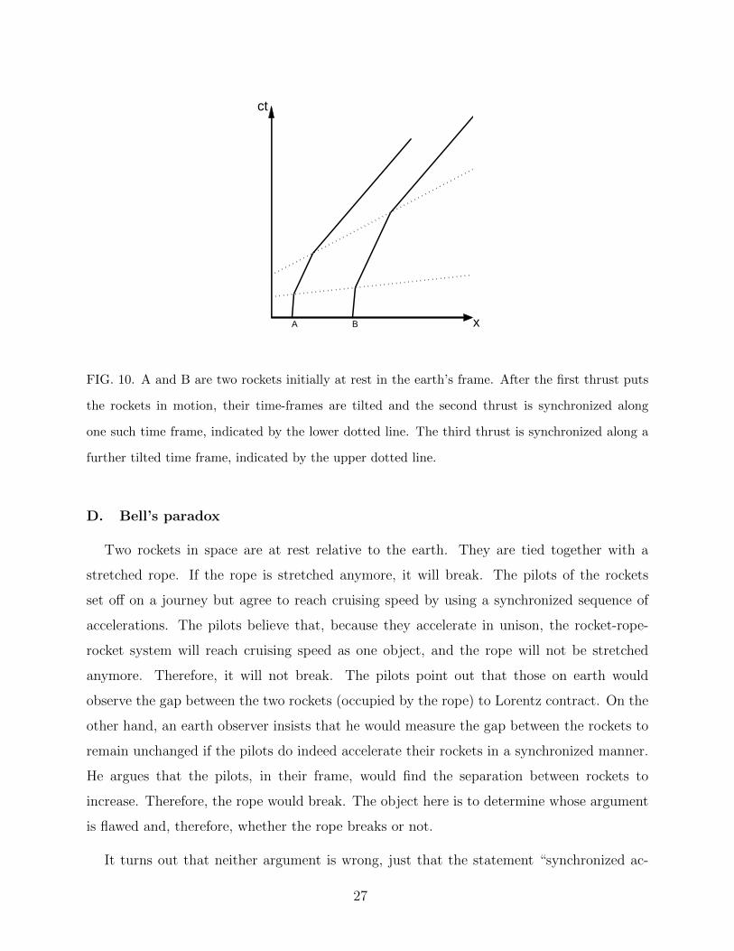
A B x

ct

FIG. 10. A and B are two rockets initially at rest in the earth’s frame. After the first thrust puts

the rockets in motion, their time-frames are tilted and the second thrust is synchronized along

one such time frame, indicated by the lower dotted line. The third thrust is synchronized along a

further tilted time frame, indicated by the upper dotted line.

D. Bell’s paradox

Two rockets in space are at rest relative to the earth. They are tied together with a

stretched rope. If the rope is stretched anymore, it will break. The pilots of the rockets

set off on a journey but agree to reach cruising speed by using a synchronized sequence of

accelerations. The pilots believe that, because they accelerate in unison, the rocket-rope-

rocket system will reach cruising speed as one object, and the rope will not be stretched

anymore. Therefore, it will not break. The pilots point out that those on earth would

observe the gap between the two rockets (occupied by the rope) to Lorentz contract. On the

other hand, an earth observer insists that he would measure the gap between the rockets to

remain unchanged if the pilots do indeed accelerate their rockets in a synchronized manner.

He argues that the pilots, in their frame, would find the separation between rockets to

increase. Therefore, the rope would break. The object here is to determine whose argument

is flawed and, therefore, whether the rope breaks or not.

It turns out that neither argument is wrong, just that the statement “synchronized ac-

27

celerations” cannot apply to both the pilots’ frame (once they start moving) and the earth

frame. If the rocket thrusts appear to be synchronized to the earth observer, the pilots’

would detect a delay between the thrusts of the two rockets. In that case, the assertion of

the earth observer, that the rope will break, will come true. In Fig. 10, we illustrate the

opposite case where the thrusts are synchronized in the pilots’ frame. The three thrusts lie

along the pilots’ lines of simultaneity at the time. In the earth frame (the stationary one),

rocket B always accelerates later, causing the gap between the two to contract. Therefore,

in this case, the rope does not break.

VI. Synopsis

Minkowski diagrams deserve a prominent place among the pedagogical tools used for

introducing special relativity to undergraduates. The graphical lessons presented here can

serve as the primary means of instruction or an alternate route available to students. The

major advantages of the methods presented here are:

1. The use of diagrams helps students visualize situations and facilitates qualitative rea-

soning. This is key to true learning and retention. The availability of graphical alter-

natives is important for enabling a more conceptual and intuitive grasp of relativity as

opposed to math-based proficiency.

2. Converting qualitative reasoning to quantitative answers requires just a few simple

steps, as outlined in section III E. The brevity of this section illustrates how easily

these diagrams can be adapted for quantitative use.

3. The usefulness of Minkowski diagrams is not limited to a subset of introductory topics.

Methods based on them are as effective and elegant as any other treatment of the

complete cannon of introductory topics, that range from Galilean transformations and

the notion of inertial observers, to deriving Lorentz transformations, time dilation,

length contraction, and other important results, to resolving difficult paradoxes in

relativity.

Our main goal has been to present, in one place, a complete set of introductory lesson plans

based on Minkowski diagrams. We have also pursued a modern and systematic approach

28

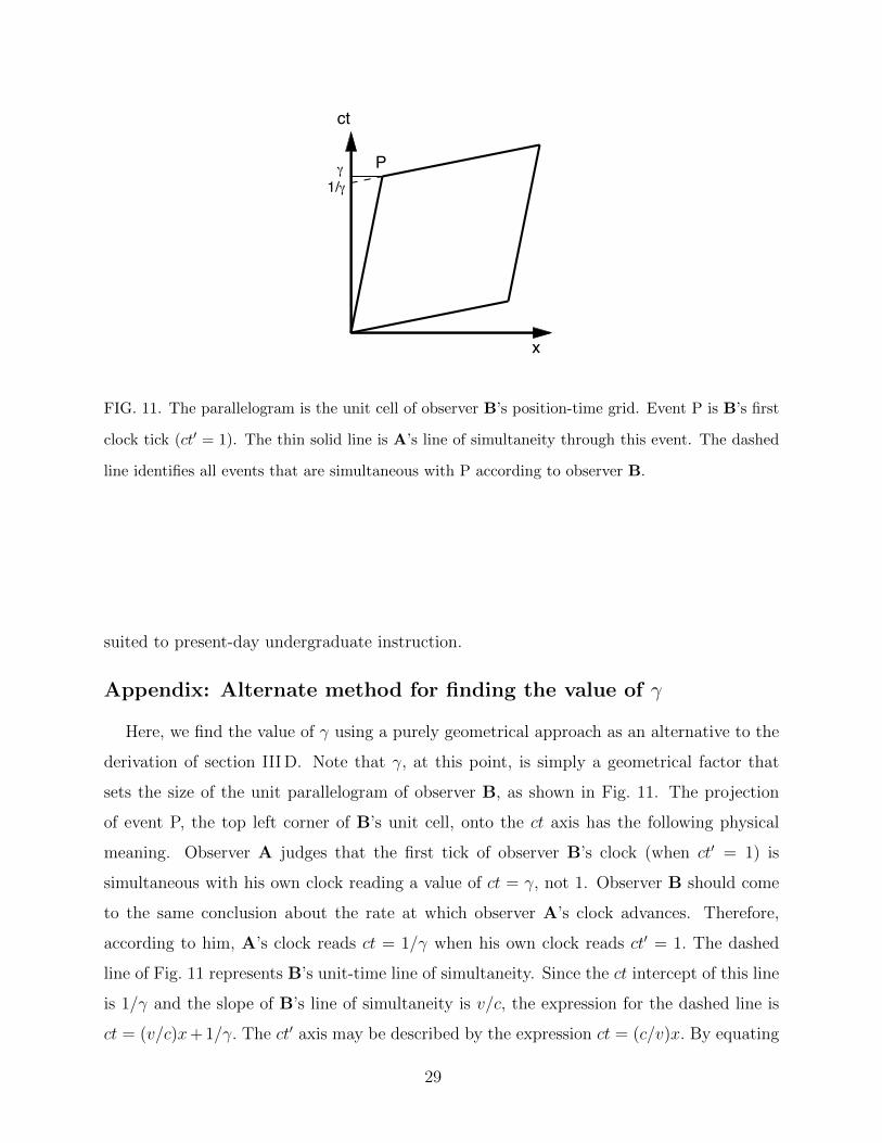
P

x

ct

γ1/γ

FIG. 11. The parallelogram is the unit cell of observer B’s position-time grid. Event P is B’s first

clock tick (ct′ = 1). The thin solid line is A’s line of simultaneity through this event. The dashed

line identifies all events that are simultaneous with P according to observer B.

suited to present-day undergraduate instruction.

Appendix: Alternate method for finding the value of γ

Here, we find the value of γ using a purely geometrical approach as an alternative to the

derivation of section III D. Note that γ, at this point, is simply a geometrical factor that

sets the size of the unit parallelogram of observer B, as shown in Fig. 11. The projection

of event P, the top left corner of B’s unit cell, onto the ct axis has the following physical

meaning. Observer A judges that the first tick of observer B’s clock (when ct′ = 1) is

simultaneous with his own clock reading a value of ct = γ, not 1. Observer B should come

to the same conclusion about the rate at which observer A’s clock advances. Therefore,

according to him, A’s clock reads ct = 1/γ when his own clock reads ct′ = 1. The dashed

line of Fig. 11 represents B’s unit-time line of simultaneity. Since the ct intercept of this line

is 1/γ and the slope of B’s line of simultaneity is v/c, the expression for the dashed line is

ct = (v/c)x+ 1/γ. The ct′ axis may be described by the expression ct = (c/v)x. By equating

29

these two expressions, we find the x-ct coordinates of event P to be

xP =v/c

γ(1− v2/c2)(A.23)

ctP =1

γ(1− v2/c2). (A.24)

But γ is defined as ctP in Fig. 11. Therefore, it follows from Eq. A.24 that γ2 = 1/(1−v2/c2).

Acknowledgments

We are indebted to Monica Moore (formerly the science division liaison of the Illinois

Wesleyan University Library and now at Notre Dame) for her untiring efforts in researching

the use of Minkowski diagrams in the literature. Her searches extended well beyond the the

period for which electronic abstracts are available.

∗ bliu2@stanford.edu

† tperera@iwu.edu

1 H. Minkowski, “Raum und Zeit,” Jahresberichte der Deutschen Mathematiker-Vereinigung,

75–88 (1909).

2 E. .F. Taylor and J. A. Wheeler, Spacetime Physics (Freeman, San Francisco 1966).

3 A. Shadowitz, Special Relativity (General Publishing, 1968).

4 Shadowitz also notes that, in comparison to other graphical approaches, this one is the most

convenient for extension to 4 dimensions and, therefore, for general relativistic applications.

5 L. Silberstein, The Theory of Relativity (MacMillan, 1914).

6 E. Loedel, “Aberracion y Relatividad,” Anales soc. cient. argentina 145, 3–13, (1948).

7 H. Amar, “New Geometric Representation of the Lorentz Transformation,” Am. J. Phys. 23,

487–489 (1955).

8 R. W. Brehme, “A Geometric Representation of Galilean and Lorentz Transformations,” Am.

J. Phys. 30, 489–496 (1962).

9 J. Rekveld, “New Aspects of the Teaching of Special Relativity,” Am. J. Phys. 37, 716–721

(1969).

30

10 M. Born, Einstein’s Theory of Relativity, revised edition (Dover, 1962). To our knowledge,

this is the text that comes closest to containing a complete graphical introduction to special

relativity through Minkowski diagrams. In it, Lorentz transformations, length contraction, and

time dilation are derived using Minkowski diagrams.

11 Some examples of excellent graphical approaches available to the community are (1) L. P.

Staunton and H. van Dam, “Graphical introduction to the special theory of relativity,” Am. J.

Phys. 48, 807–817 (1980). (2) S. C. Daubin, “A geometrical introduction to special relativity,”

Am. J. Phys. 30, 818-824 (1963). (3) R. de Abreu and V. Guerra, “Special relativity as a simple

geometry problem,” Eu. J. Phys. 30, 229-237 (2009).

12 Penha and Rothstein, <arXiv:physics/0703002>; Penha, Rothstein, and Paunescu, <arXiv:

0706.2123>; Herman, <http://people.uncw.edu/hermanr/GR/Minkowski/Minkowski.pdf>;

Turley, <http://www.physics.byu.edu/faculty/allred/222%2011/minkowski%2011.pdf>;

and a web tutorial at <http://lgsims96.hubpages.com/hub/Minkowski-Diagram>. There is

even a YouTube video at <http://www.youtube.com/watch?v=bPxvUW1S2k> and an interactive

tutorial at <www.trell.org/div/minkowski.html>.

13 For instance, in the textbooks by Born and by Taylor and Wheeler, cited above.

14 Particularly in connection with graphical derivations of the relativistic Doppler effect as in (1)

R. E. Reynolds, “Doppler effect for sound via classical and relativistic space-time diagrams,”

Am. J. Phys. 58, 390–394 (1990). and (2) G. Cook and T. Lesoing, “A simple derivation of the

Doppler effect for sound,” Am. J. Phys. 59, 218–220 (1991).

15 We want to emphasize here that γ at this point has no physical meaning. It is simply a geomet-

rical scaling factor.

16 This is true because the ct′ axis is also the worldline of the left end of the ruler TP.

17 Actually, according to the earth-bound twin, the astronaut twin ages slightly faster near the

turn-around, because the slope of her worldline is changing. For instance, when the astronaut’s

worldline is vertical, both twins age at the same rate.

31