A goal-seeking approach to capital budgeting

Socio-Economic Planning Sciences 39 (2005) 165–182

A goal-seeking approach to capital budgeting

Yupo Chana,*, Joseph P. DiSalvob, Michael W. Garrambonec

aDepartment of Systems Engineering, University of Arkansas, 2801 South University, Little Rock, AR 72204-1099, USAb2828 Scarborough Drive, Richmond, VA 23235, USA

cVeridian Engineering, 5200 Springfield Pike, Dayton, OH 45431-1255, USA

Available online 17 June 2004

Abstract

This paper articulates how a goal-seeking model addresses a variation of the capital-budgeting problem.Focused toward technology modernization in the public sector, this multi-criteria optimization modelexplicitly considers the diverse functions of the organization. In particular, the synergism amongst thefunctions is modeled as a multiplicative value function. The model is solved by the ‘‘constraint reducedfeasible-region method’’, resulting in a non-convex mathematical program that produces numericalintricacies. Linearization of the criterion (objective) functions reduces such intricacy. An Army-modernization acquisition-study was used to illustrate the proposed model, showing that its non-inferiorsolutions are remarkably stable. Comparison is also made with other approaches, typically formulated asgoal-setting programs. The model highlights how technology acquisitions are affected as the priorities ofeach organizational function changes.r 2004 Elsevier Ltd. All rights reserved.

Keywords: Project selection; Multicriteria optimization; Value functions; Technology modernization

1. Introduction

The capital-budgeting problem [1], also known as the project selection problem, specifies a subsetof programs, projects, investment packages, etc., within budgetary and other resource limitations.Going beyond a single budget cycle, budgeting and procurement decisions over time must beconsidered. A simple capital-budgeting problem can be formulated using linear integer-programming with binary variables. Each candidate project i has an associated value vi,representing the merit of the project. Estimating these values, however, is not simple, since it is a

ARTICLE IN PRESS

*Corresponding author. Tel.: +1-501-569-3100; fax: +1-501-569-8698.

E-mail address: [email protected] (Y. Chan).

0038-0121/$ - see front matter r 2004 Elsevier Ltd. All rights reserved.

doi:10.1016/j.seps.2004.04.002

composite of several criteria—the classic ‘‘apples’’ vs. ‘‘oranges’’ tradeoff problem. A technique toestimate such values involves using several criteria or objective functions, each modeling adifferent valuation of merit. Goal programming is commonly used, in which an aspiration level isspecified for each criterion.Challenging as it may be, this type of problem is common in the procurement scheduling of

many organizations, both public and private. Faced with multiple functional requirements, suchorganizations typically consider many of the following factors [2]:

* Procurement schedule,* Technology mix (old and new) by composition by year,* Technology composition by cohort time-periods,* Annual expenditure,* Retirement schedule by technology system,* Retirement schedule by cohort time-periods,* Mission requirements for systems,* Average age of a technology system,* Fraction of high-technology modernization, and* Production-line capacity utilization.

Brown et al. [2] used a mixed-integer linear-programming (MILP) model to plan for a 25-yearArmy procurement schedule. Several factors, including costs, force-structure requirements,resources available and vehicle life were incorporated into their MILP model. The model, in turn,produced procurement and retirement schedules, changes to force composition, and procurementexpenditures. The model minimized operating and maintenance costs subject to various goalconstraints. Each requirement in the constraint was stated as an aspiration or goal.Loerch et al. [3] used a value-added-analysis (VAA) model to bring new technology into the

Army inventory. VAA uses a family of simulation, statistical, and decision-analytic models toestimate the value added and costs of various procurement programs. Typically, optimizationtechniques are then applied to identify a theoretically desirable mix of systems and equipment.Parametric analysis was used in [3] to evaluate tradeoffs between systems. An alternate approachwould have been to rank alternative systems for each military functional area and then coordinateamongst them to arrive at a consensus. Since consensus building is often a difficult task, Loerchproposed VAA be used. The unique feature of VAA is that it defines the issues and criteria at theoutset of the analysis.Recognizing the challenges in estimating the value of a project, Jackson et al. [4] used decision

analysis to select a set of optimal projects. The measures supporting their objectives were clearlyidentified as risk, life-cycle cost, and time for implementation. Their model used exponential,univariate utility-functions vi(xi) to quantify these measures xi within an additive value-functionf(x):

f ðxÞ ¼ w1v1ðx1Þ þ w2v2ðxÞ þ?þ wmvmðxmÞ: ð1Þ

Here, wi are the weights placed on each measure or utility function, with Si wi = 1. They usedcumulative frequency distributions for risk, cost, and time to illustrate the dominance oftechnology choices. A portfolio of technologies was captured, allowing the decision makers to

ARTICLE IN PRESS

Y. Chan et al. / Socio-Economic Planning Sciences 39 (2005) 165–182166

consider the continual funding of several attractive, competing technologies while eliminatingthose that were clearly dominated.The above are only three of a myriad of studies in the area of project selection. They clearly

illustrate the complexity of valuating a project. For the curious reader, other discussions are foundin [5–11].

2. The multi-period technology modernization problem

A general technology-modernization model that explicitly evaluates mission effectivenessis desired. A public-sector focused model is characterized by the following attributes (amongothers) [1]:

(a) Mission statements are required to be explicit and subject to critical public scrutiny.(b) Significant pressures are exerted from technology suppliers and from pluralistic constituencies

during public debate.(c) Budgetary considerations are rigidly defined ahead of time.

A classic capital-budgeting formulation has binary (indicator) variables to decide if a project isfunded or not. The supplier’s production schedule will deliver the acquired units within a timewindow. This window is typically marked by another binary variable. Due to the productioncapacity of a supplier, there exists a limit on the production of the ith-type units. There is a specificsequence of production lines required for these units. A contingent relationship is often placedbetween selected production lines. For example, if production line l is closed in time t, thenproduction line l0 must open in time t +1, or not at all. These represent the logical conditionsplaced on interdependent projects in a capital-budgeting model.In our model, a continuous variable tracing an inventory was used. Thus, xic(t) denotes the

operational units of technology-type i of cohort-year c in time t. Here, a cohort year distinguishesbetween a ‘‘first generation’’ widget vis-a-vis a ‘‘second generation’’ widget. Rather than using adiscrete integer variable to account for the widgets, a continuous variable was employed.Discretization is sometimes required to distinguish between buying one vs. two widgets. However,when acquisitions are in large numbers, the difference between buying, say, 3871 vs. 3870.5widgets is probably insignificant.Cash flow can conveniently be used, should one decide to convert all inventory into dollars. In

our model, a modernization schedule had to be implemented either by explicitly defining the type-iunits retired at time t in a cohort-group c, or implicitly by tracing the value of xic(t) over time t.Thus, when xic(2) is half the value of xic(1), it means that half the type-i units in cohort-group c

would be retired between years 1 and 2.A constraint was used to suggest that sufficient ith type units be available at time t. An age

limitation is often placed on retiring units from the existing inventory. The available budget isspecified in this case. Sometimes, a minimal expenditure threshold is required, suggesting that theorganization be obligated to spend a certain amount of money on a technology. Standardproduction/inventory balance equations were thus modified to show the attrition from one timeperiod to the next. Some constraints can be elastic, suggesting that they can be violated. Thus,

ARTICLE IN PRESS

Y. Chan et al. / Socio-Economic Planning Sciences 39 (2005) 165–182 167

when production capacity was exceeded, a linear cost per extra unit produced was imposed as apenalty, suggesting overtime pay. These elastic constraints are typical in a goal programming (GP)model, where a goal can be under-achieved or exceeded, as indicated by the deviation variables di

�

and di+ respectively. In this context, a goal-setting MILP model was defined as

minXq

i¼1

ðd�i þ dþ

i Þp ¼

Xq

i¼1

jiðdiÞ ð2Þ

s.t.

y�i � fiðxÞ � d�i ¼ dþ

1 ði ¼ 1; y; qÞ; xAX :

Here, y�i represents the goal or functional requirement set for criterion i. fi(x) is the criterionfunction and xAX is the linear decision space. No weights are placed on the deviation functionsji (di) in this formulation. When p =1, it represents a regular linear goal-program [11,12]. It canbe shown that goal-setting programs are special cases of the goal-seeking program, when the valuefunction f(x) = V [ f1(x), f2(x),y, fq(x)] assumes an lp-metric form [13].

3. Portfolio valuation and selection

Using the language of multi-attribute decision analysis, each criterion or objective function in amathematical program is a form of value function. Often, technologies used for a commonmission will be more valuable when applied in tandem than apart. All possible interaction terms inthis value function are to be included. The assumptions of mutual-preferential-independence andmutual-utility-independence together imply that a joint utility function may be expressed as afunction of the marginal (univariate) utility functions. The form f(x1,y,xq) = V[v1(x1),y,vq(xq)]was thus adopted here. For current purposes, the f ( � ) is decomposable into function V( � ) asdefined by the following multiplicative expression [14]:

kf ðxÞ þ 1 ¼Ym

i¼1

½1þ kwiviðxiÞ: ð3Þ

A salient feature of this decomposition is that a minimal number of calibration parameters isrequired. For example, a two-attribute utility function can be calibrated with two parameters P1

and P2 as follows:

f ðx1;x2Þ ¼ w1v1ðx1Þ þ w2v2ðx2Þ þ kw1w2v1ðx1Þv2ðx2Þ

¼ P1v1ðx1Þ þ P2v2ðx2Þ þ ð1� P1 � P2Þv1ðx1Þv2ðx2Þ: ð4Þ

For three attributes, the multivariate function assumes the form

f ðx1;x2; x3Þ ¼w1v1ðx1Þ þ w2v2ðx2Þ þ w3v3ðx3Þ þ kw1w2v1ðx1Þv2ðx2Þ þ kw1w3v1ðx1Þv3ðx3Þ

þ kw2w3v2ðx2Þv3ðx3Þ þ k2w1w2w3v1ðx1Þv2ðx2Þv3ðx3Þ: ð5Þ

Expression (4) (and its higher-dimensional generalizations) exemplify the most generalrepresentation of a multi-attribute utility-function, considering the efficiency with which suchfunctions can be calibrated [14]. In fact, Eq. (1) is a special case of Eq. (3) when no interactionterm exists (i.e., k = 0).

ARTICLE IN PRESS


Having defined function (3) for the relevant criteria yi = fi (x), we formulate a nonlinear multi-criteria optimization problem as follows:

fmax f1ðxÞ; max f2ðxÞ;y; max fqðxÞjxAXg: ð6Þ

Notice that now we have a goal-seeking model rather than a goal-setting model. Each criterioncan thus be a mission of an organization. This approach differs from others such as [2] in that nowwe use a mission-oriented analysis (MOA). Such analysis is more objective in nature and lesscontroversial than subjective assessments such as specifying goal aspiration levels yi

�.MOA requires that we begin with a statement of goals and objectives. For example, assume we

wish to acquire brand-X and brand-Y widgets to provide the best public service at the lowest costto the tax payers. Contrast this with a direct tradeoff between technology systems, such asexplicitly maximizing the number of low-cost X widgets and minimizing the number of high-costY widgets. The former explicitly recognizes the mission of the organization while the latter doesnot.Now, recall that xic denote the number of units of technology-type i acquired in cohort-year

group c. Yearly budget constraints accounting for both production costs a (which includesresearch and development) and operating/maintenance costs b are written for all technology-type i

and cohort-year groups c. This first set of constraints appears as follows:XiAiðtÞ

XcAcðtÞ

aixic þX

iAiðt�1Þ

XcAcðt�1Þ

bixicrBt ðt ¼ 1; 2; 3;yÞ: ð7Þ

Here, the set of technologies i(t) and cohort-group c(t) are specified for each year t. Notice that thetechnologies acquired in a previous year, t�1, have to be maintained in current year t within thecurrent year budget Bt.Modernization-mission constraints specify the range between the minimum Lt and maximum

Ut size required among all technology-types i and cohort-groups c in each year t. This condition isgiven in

UtZ

XiAi0

XcAc0ðtÞ

xicZLt ðt ¼ 1; 2; 3;yÞ: ð8Þ

Again, the actively considered technologies i0(t) and cohorts c0(t) are specified for each year t.These technologies and cohorts need not be the same as those defined in the first constraint set (7).Production constraints limit the number of technology-i and cohort-group c units that can be

produced in year t, as modeled in

xi00ðtÞ;c00ðtÞrPi ðfor all technology-types i00ðtÞ and cohort-groups c00ðtÞ; t ¼ 1; 2; 3;yÞ: ð9Þ

Here, pertinent technology-types i00(t) and cohort-groups c00(t) are uniquely defined for each year t.Availability constraints (10) suggest the minimum production of each technology type for a

cohort-year group:

xi000ðtÞ;c000ðtÞZAt ðfor all technology-types i000ðtÞ and cohort-groups c000ðtÞ; t ¼ 1; 2; 3;yÞ:

ð10Þ

Notice that the technology-types and cohort-groups are again defined differently from theproduction limitation constraints.

ARTICLE IN PRESS


Technology needs specify the minimum production threshold of each technology i for thecohort years c, as given inX

cot

xi0000ðtÞ;cZTt ðfor all technology-type i0000ðtÞ; t ¼ 1; 2; 3;yÞ: ð11Þ

Notice that all cohort groups before year t are considered here.Finally, it is entirely possible that some of the above sets of constraints are redundant. Amongst

the redundant constraints, obviously the most binding would apply.

4. A goal-seeking additive value-function formulation

Having formulated the above portfolio-selection model, we quantify the missions in our MOA.Before delving into a case study, we also wish to point out some analytical features of such anMOA. Suppose the univariate value functions vi(xi) = xi, and f(x) assume the form of Eq. (1). Wethen have an additive linear value-function that may be an approximation of Eq. (4) and theirhigher-dimension generalizations. Here, we assume adaptivity and proportionality. Adaptivitymeans that the impact of technology systems is the sum of the performance of each componentsystem rather than the synergistic effects amongst them. By proportionality, we mean that twicethe number of systems would result in twice the effectiveness. In other words, we are operatingsolely in a linear domain.We emphasize here that the ranking among alternatives will be the same whether an additive or

multiplicative function is used, as long as they are strategically equivalent [14]. Any value functioncan be transformed by a monotonic function and the result will represent the same preferences asbefore. This applies to multi-criteria optimization as well, in which the set of non-dominatedsolutions remains the same for strategically equivalent criteria.We recall that when k=0 in Eq. (5), the multiplicative function reduces to the simple additive

form, with w1+ w2 +?+ wm=1. We say that the vi(xi) = yi exhibit additive independence in thiscase. What happens if two criteria fi(x) and fj(x) used in an analysis are correlated instead ofindependent? Obviously, the above two-step process of (a) measuring a univariate function, and(b) aggregating them into a multivariate one will no longer be valid. Additional analysis must beincorporated into forming a multi-attribute value-function.In multi-criteria optimization, not all fi(x) in the objective function V ( f1(x),y, fq(x)) can be

independent. Independence in this context means that the fi(x) are orthogonal. Consider twolinear criteria fi (x) = (ci )T x and fj (x)= (c j )T x. A measure for the correlation between the ithand jth criteria is similar to its statistical analogue. The angle between the two criterion vectors isdefined between the gradients c i and c

j:

cos�1ðciÞTcj

jjcijj2jjcj jj2

� �: ð12Þ

An ideal angle is 90 when the two criteria are totally independent. The more the criteria arecorrelated, the smaller the angle.In the Army case study immediately below (Section 5), for example, a check on the

interdependence of criteria 1 and 2 shows that the two criterion functions are independent of one

ARTICLE IN PRESS


another. The correlation angle is shown to be 84.5 , which puts them into an acceptable level ofindependence. In other words, they are orthogonal to one another to such an extent that theformulation cited above would be valid.The multi-parametric decomposition technique is employed in this case study to examine the

non-dominated set of solutions [15]. In this regard, the analysis identifies a portfolio ofalternatives for decision makers rather than selecting the ‘‘optimal’’ one. The multi-parametricdecomposition technique operates on three planes: the feasible region X, outcome space Y, and Zspace. The feasible region is the domain in which the decision variables, such as the units oftechnology type i, are found. The outcome space is the domain in which the criteria are defined.The Z space is where tradeoffs are made between the two criteria identified without the use ofweights. The idea is to identify some sets of non-dominated alternatives that would support bothcriteria without specifying weights for one vs. the other.

5. The case study

A review of the US Army vehicle-acquisition process has shown that the ideology before 1986was based upon single system impacts. In other words, analysis focused on the effect ofintroducing an additional system into the inventory within the acquisition plan. This type ofanalysis has been repeated for all candidate systems, resulting in a prioritization among proposedsystems. Since 1986, emphasis has been on combined systems impacts, as illustrated by the air-land-battle future concept, where several systems—both on ground and in the air—are configuredtogether to accomplish a specified mission. The Army aviation-modernization tradeoff-requirement study [2], as cited in the literature review, is an example of this focus. Othersuch studies have been described above, in Section 1, including VAA, and collaborative analyses[7,9].

5.1. Army acquisition goals

A major technological concern of the US Army is to plan for their fleet, ranging from heavy tolight armored vehicles. This represents a significant multi-year capital-budgeting problem. Wepresent a goal-seeking approach to model the injection of future vehicles to replace existing Armyinventory. Lethal weapons systems are getting smarter and lighter. To accommodate this trend,the Army launched the heavy force modernization (HFM) program. Here, we begin with goalsand objectives of the HFM program, and deduce the resulting combat-vehicle acquisition overtime [7]. By stating combat missions explicitly, the required weapon inventory to fight future warscan be specified. This way, one avoids patronizing debates amongst weapon systems such as:‘‘tanks are more important than howitzers,’’ or vice versa.A key concept in today’s battlefield is the coordination between air power and ground forces. In

1990, the Program Integration Office of the Training and Doctrine Command was interested intranslating such an ‘‘air–land battle future concept’’ into a program of combat-vehicle acquisitionover multiple years [6]. Integration of the assault and assault-fire support missions is a keydoctrine of the air–land battle future. Assault-fire support could include aircraft in addition tologistic vehicles such as fuel trucks.

ARTICLE IN PRESS


The HFM program, similar to other major acquisition programs, is concerned with a myriad offactors. Among softer issues are the economic and political pressures brought on bymanufacturers in different geographic locations of the country, and the expected debates thatgo on in a pluralistic democracy. For these reasons, we were not able to obtain the detailed data,as they were not releasable to the public at the time of the study. In our example, only arepresentative data set was thus used. A prototype model was created that required minimalessential data input. Rather than producing a detailed acquisition plan over time, we highlight thetradeoffs among missions. The purpose of the prototype was to expedite decision making and tostimulate further development of the model into a more detailed production version at a laterdate.

5.2. A mission-oriented model

As mentioned, our approach is goal-seeking rather than goal-setting. Unlike other operations,it is felt that the Army’s new integrated concept is too developmental to allow a well-establishedstandard to be applied. Simply put, no standards exist for missions such as combat and combat-fire support to allow goal-setting. The multi-parametric decomposition technique, as defined at theend of Section 4, is thus employed to examine the non-dominated set of solutions. The analysisidentifies a portfolio of non-inferior alternatives for decision makers rather than selecting an‘‘optimal’’ one. Again, the focus is to identify the comprehensive set of alternatives that wouldsupport both criteria, accounting for all weight distributions placing one criterion vis-a-visanother.Below are the specific data requirements for the general model, Eqs. (6)–(11) above. For the

budget constraint (7), we need:

* unit production cost per vehicle (including research, development, testing and evaluation) a;* current vehicle inventory, iA i(t) and cA c(t); and* operations and maintenance cost per vehicle, b.

For the mission constraint (8), we require:

* number of vehicles needed per technology type, iA i0(t); and* current vehicle inventory, iA i0(t) and cA c0(t).

For the production constraints (9) and (10), we assemble:

* total capacity of production facilities Pt;* production threshold At; and* production-facility operational time-line for technology-type i and cohort-group c, i00(t), c00(t),

i000(t), and c000(t).

And, finally, for the technology-needs constraint (11), we gather:

* number of ‘‘high-tech’’ vehicles types i000(t); and* the year a ‘‘high-tech’’ vehicle is considered, t>c.

Recall that xic denotes the vehicle type i acquired in cohort year c. Two sets of decisionvariables are defined—for the existing heavy-force vehicles and the HFM vehicles—consisting of

ARTICLE IN PRESS


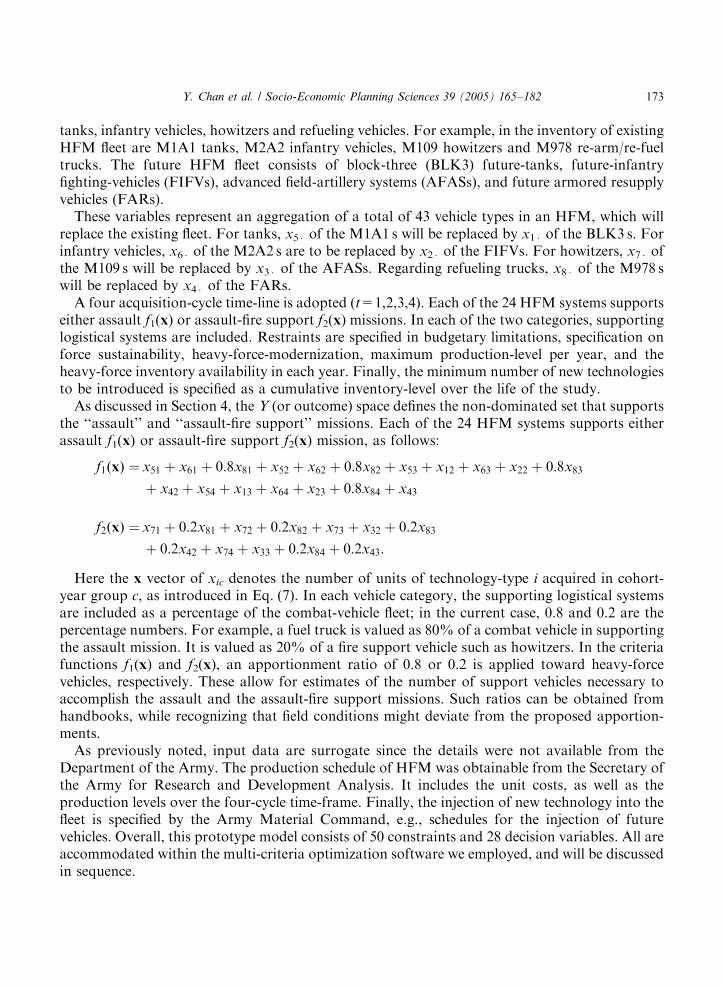
tanks, infantry vehicles, howitzers and refueling vehicles. For example, in the inventory of existingHFM fleet are M1A1 tanks, M2A2 infantry vehicles, M109 howitzers and M978 re-arm/re-fueltrucks. The future HFM fleet consists of block-three (BLK3) future-tanks, future-infantryfighting-vehicles (FIFVs), advanced field-artillery systems (AFASs), and future armored resupplyvehicles (FARs).These variables represent an aggregation of a total of 43 vehicle types in an HFM, which will

replace the existing fleet. For tanks, x5 � of the M1A1 s will be replaced by x1 � of the BLK3 s. Forinfantry vehicles, x6 � of the M2A2 s are to be replaced by x2 � of the FIFVs. For howitzers, x7 � ofthe M109 s will be replaced by x3 � of the AFASs. Regarding refueling trucks, x8 � of the M978 swill be replaced by x4 � of the FARs.A four acquisition-cycle time-line is adopted (t=1,2,3,4). Each of the 24 HFM systems supports

either assault f1(x) or assault-fire support f2(x) missions. In each of the two categories, supportinglogistical systems are included. Restraints are specified in budgetary limitations, specification onforce sustainability, heavy-force-modernization, maximum production-level per year, and theheavy-force inventory availability in each year. Finally, the minimum number of new technologiesto be introduced is specified as a cumulative inventory-level over the life of the study.As discussed in Section 4, the Y (or outcome) space defines the non-dominated set that supports

the ‘‘assault’’ and ‘‘assault-fire support’’ missions. Each of the 24 HFM systems supports eitherassault f1(x) or assault-fire support f2(x) mission, as follows:

f1ðxÞ ¼ x51 þ x61 þ 0:8x81 þ x52 þ x62 þ 0:8x82 þ x53 þ x12 þ x63 þ x22 þ 0:8x83

þ x42 þ x54 þ x13 þ x64 þ x23 þ 0:8x84 þ x43

f2ðxÞ ¼ x71 þ 0:2x81 þ x72 þ 0:2x82 þ x73 þ x32 þ 0:2x83

þ 0:2x42 þ x74 þ x33 þ 0:2x84 þ 0:2x43:

Here the x vector of xic denotes the number of units of technology-type i acquired in cohort-year group c, as introduced in Eq. (7). In each vehicle category, the supporting logistical systemsare included as a percentage of the combat-vehicle fleet; in the current case, 0.8 and 0.2 are thepercentage numbers. For example, a fuel truck is valued as 80% of a combat vehicle in supportingthe assault mission. It is valued as 20% of a fire support vehicle such as howitzers. In the criteriafunctions f1(x) and f2(x), an apportionment ratio of 0.8 or 0.2 is applied toward heavy-forcevehicles, respectively. These allow for estimates of the number of support vehicles necessary toaccomplish the assault and the assault-fire support missions. Such ratios can be obtained fromhandbooks, while recognizing that field conditions might deviate from the proposed apportion-ments.As previously noted, input data are surrogate since the details were not available from the

Department of the Army. The production schedule of HFM was obtainable from the Secretary ofthe Army for Research and Development Analysis. It includes the unit costs, as well as theproduction levels over the four-cycle time-frame. Finally, the injection of new technology into thefleet is specified by the Army Material Command, e.g., schedules for the injection of futurevehicles. Overall, this prototype model consists of 50 constraints and 28 decision variables. All areaccommodated within the multi-criteria optimization software we employed, and will be discussedin sequence.

ARTICLE IN PRESS


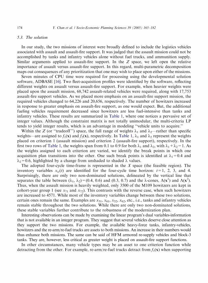
5.3. The solution

In our study, the two missions of interest were broadly defined to include the logistics vehiclesassociated with assault and assault-fire support. It was judged that the assault mission could not beaccomplished by tanks and infantry vehicles alone without fuel trucks, and ammunition supply.Similar arguments applied to assault-fire support. In the Z space, we left open the relativeimportance of assault versus assault-fire support. In this regard, multi-parametric decompositionmaps out consequences of any prioritization that one may wish to place upon either of the missions.Seven minutes of CPU time were required for processing using the developmental solution

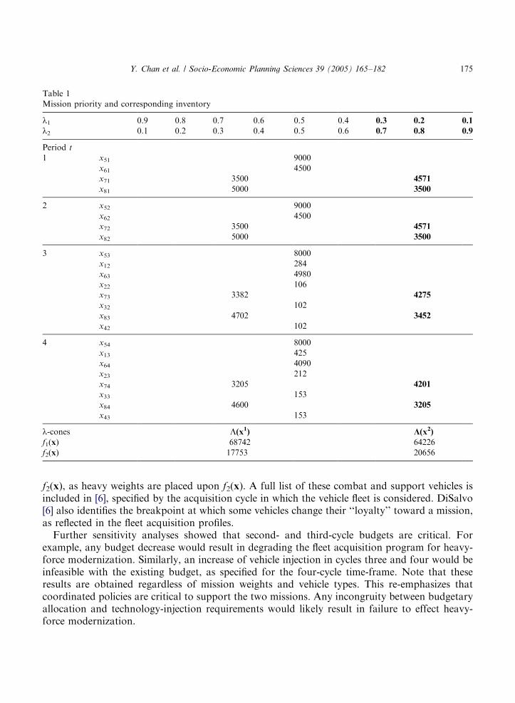
software, ADBASE [16]. Two fleet-acquisition profiles were identified by the software, reflectingdifferent weights on assault versus assault-fire support. For example, when heavier weights wereplaced upon the assault mission, 68,742 assault-related vehicles were required, along with 17,753assault-fire support vehicles. As we placed more emphasis on an assault-fire support mission, therequired vehicles changed to 64,226 and 20,656, respectively. The number of howitzers increasedin response to greater emphasis on assault-fire support, as one would expect. But, the additionalfueling vehicles requirement decreased since howitzers are less fuel-intensive than tanks andinfantry vehicles. These results are summarized in Table 1, where one notices a pervasive set ofinteger values. Although the constraint matrix is not totally unimodular, the multi-criteria LPtends to yield integer results, which is an advantage in modeling ‘‘vehicle units to acquire.’’Within the Z (or ‘‘tradeoff ’’) space, the full range of weights l1 and l2—rather than specific

weights—are assigned to f1(x) and f2(x), respectively. In Table 1, l1 and l2 represent the weightsplaced on criterion 1 (assault mission) and criterion 2 (assault-fire support), respectively. In thefirst two rows of Table 1, the weights span from 0.1 to 0.9 for both l1 and l2, with l1+l2=1. Asthe weights assigned to each criterion are varied, we identify the break points in which oneacquisition plan transitions into the other. One such break points is identified at l1=0.4 andl2=0.6, highlighted by a change from unshaded to shaded l values.The adopted four-cycle time-frame is represented in the X space (the feasible region). The

inventory variables xic(t) are identified for the four-cycle time horizon: t=1, 2, 3, and 4.Surprisingly, there are only two non-dominated solutions, delineated by the vertical line thatseparates the table between (l1, l2)=(0.4, 0.6) and (0.3, 0.7) and the l-cones, L(x1) and L(x2).Thus, when the assault mission is heavily weighted, only 3500 of the M109 howitzers are kept incohort-year group 1 (see x71 and x72). This contrasts with the reverse case, when such howitzersare increased to 4571. While most of the inventory variables change between these two solutions,certain ones remain the same. Examples are x51, x61, x52, x62, etc., i.e., tanks and infantry vehiclesremain stable throughout the two solutions. While there are only two non-dominated solutions,these stable variables further contribute to the robustness of the modernization plan.Interesting observations can be made by examining the linear program’s dual variables-information

that is not available in an integer program. They suggest that several vehicles deserve close attention asthey support the two missions. For example, the available heavy-force tanks, infantry-vehicles,howitzers and the re-arm/re-fuel trucks are assets to both missions. An increase in their numbers wouldthus enhance both missions. The same can be said of HFM armored re-supply vehicles and block-3tanks. They are, however, less critical as greater weight is placed on assault-fire support functions.In other circumstances, many vehicle types may be an asset to one criterion function while

detracting from the other. For example, re-arm/re-fuel trucks detract from f1(x) when supporting

ARTICLE IN PRESS


f2(x), as heavy weights are placed upon f2(x). A full list of these combat and support vehicles isincluded in [6], specified by the acquisition cycle in which the vehicle fleet is considered. DiSalvo[6] also identifies the breakpoint at which some vehicles change their ‘‘loyalty’’ toward a mission,as reflected in the fleet acquisition profiles.Further sensitivity analyses showed that second- and third-cycle budgets are critical. For

example, any budget decrease would result in degrading the fleet acquisition program for heavy-force modernization. Similarly, an increase of vehicle injection in cycles three and four would beinfeasible with the existing budget, as specified for the four-cycle time-frame. Note that theseresults are obtained regardless of mission weights and vehicle types. This re-emphasizes thatcoordinated policies are critical to support the two missions. Any incongruity between budgetaryallocation and technology-injection requirements would likely result in failure to effect heavy-force modernization.

ARTICLE IN PRESS

Table 1

Mission priority and corresponding inventory

l1 0.9 0.8 0.7 0.6 0.5 0.4 0.3 0.2 0.1

l2 0.1 0.2 0.3 0.4 0.5 0.6 0.7 0.8 0.9

Period t

1 x51 9000

x61 4500

x71 3500 4571

x81 5000 3500

2 x52 9000

x62 4500

x72 3500 4571

x82 5000 3500

3 x53 8000

x12 284

x63 4980

x22 106

x73 3382 4275

x32 102

x83 4702 3452

x42 102

4 x54 8000

x13 425

x64 4090

x23 212

x74 3205 4201

x33 153

x84 4600 3205

x43 153

l-cones L(x1) K(x2)

f1(x) 68742 64226

f2(x) 17753 20656


5.4. Remarks

In the authors’ view, the individual vehicle-type approach to analyzing HFM is not entirelysatisfactory. The reason is that it represents an outdated notion of having priorities being placedon individual vehicle fleets. It contradicts current war-fighting doctrine that coordinates force-structure to support stated missions. In this study we adopted a mission-oriented analysis, whichadequately portrayed the synergism required in air–land battle future concept. In this model, wesupported combined arms-operations with a multi-criteria rather than a single-criterion model.The model is aggregate in nature. It portrays fundamental missions and tradeoffs. Thisformulation could be extended by considering a comprehensive set of factors, albeit under theweight of computer run time and extensive data requirements. But, our analysis shows that multi-parametric decomposition incorporated mission prioritization and specified a HFM vehicle-acquisition schedule over a four-cycle time-horizon both effectively and efficiently.While our aggregate model serves its function rather well, future extensions as alluded to above

may be desirable to produce production (rather than prototype) runs. First, one may wish tobreak down the budget into more detailed levels; e.g., by considering operation and maintenancecosts in terms of more detailed factors such as fuel, repair, etc. More attention could also beplaced on logistical apportionment issues; e.g, by basing it on fuel and ammunition consumption.In tanks and infantry vehicles, the assault-mission vehicles consume more fuel than howitzers intheir assault-fire support mission. However, howitzers consume more ammunition than tanks andinfantry vehicles. A further complication could occur when one logistical vehicle is used for bothre-arming and re-fueling.

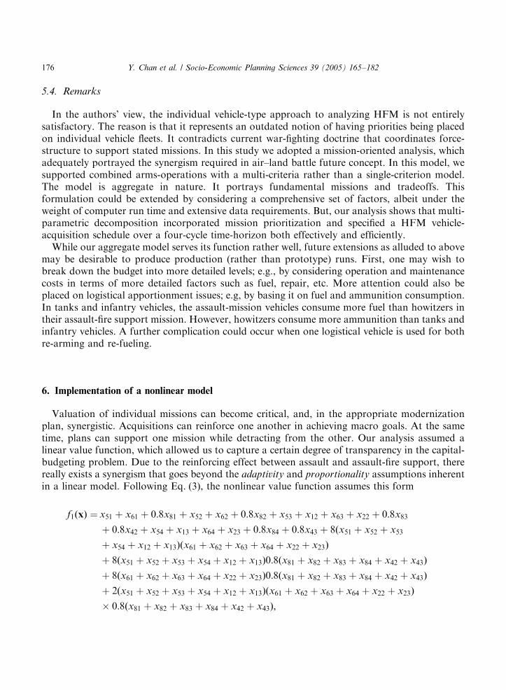
6. Implementation of a nonlinear model

Valuation of individual missions can become critical, and, in the appropriate modernizationplan, synergistic. Acquisitions can reinforce one another in achieving macro goals. At the sametime, plans can support one mission while detracting from the other. Our analysis assumed alinear value function, which allowed us to capture a certain degree of transparency in the capital-budgeting problem. Due to the reinforcing effect between assault and assault-fire support, therereally exists a synergism that goes beyond the adaptivity and proportionality assumptions inherentin a linear model. Following Eq. (3), the nonlinear value function assumes this form

f1ðxÞ ¼ x51 þ x61 þ 0:8x81 þ x52 þ x62 þ 0:8x82 þ x53 þ x12 þ x63 þ x22 þ 0:8x83

þ 0:8x42 þ x54 þ x13 þ x64 þ x23 þ 0:8x84 þ 0:8x43 þ 8ðx51 þ x52 þ x53

þ x54 þ x12 þ x13Þðx61 þ x62 þ x63 þ x64 þ x22 þ x23Þ

þ 8ðx51 þ x52 þ x53 þ x54 þ x12 þ x13Þ0:8ðx81 þ x82 þ x83 þ x84 þ x42 þ x43Þ


þ 2ðx51 þ x52 þ x53 þ x54 þ x12 þ x13Þðx61 þ x62 þ x63 þ x64 þ x22 þ x23Þ

� 0:8ðx81 þ x82 þ x83 þ x84 þ x42 þ x43Þ;

ARTICLE IN PRESS


f2ðxÞ ¼ x71 þ 0:2x81 þ x72 þ 0:2x82 þ x73 þ x32 þ 0:2x83 þ 0:2x42 þ x74 þ x33 þ 0:2x84 þ 0:2x43


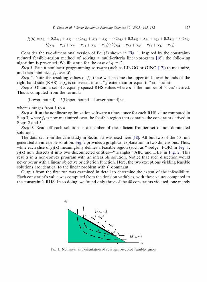
Consider the two-dimensional version of Eq. (3) shown in Fig. 1. Inspired by the constraint-reduced feasible-region method of solving a multi-criteria linear-program [16], the followingalgorithm is presented. We illustrate for the case of q = 2.

Step 1. Run a nonlinear-programming software (such as LINGO or GINO [17]) to maximize,and then minimize, f2 over X.

Step 2. Note the resulting values of f2; these will become the upper and lower bounds of theright-hand side (RHS) as f2 is converted into a ‘‘greater than or equal to’’ constraint.

Step 3. Obtain a set of n equally spaced RHS values where n is the number of ‘slices’ desired.This is computed from the formula

ðLower boundÞ þ i ðUpper bound� Lower boundÞ=n;

where i ranges from 1 to n.Step 4. Run the nonlinear optimization software n times, once for each RHS value computed in

Step 3, where f1 is now maximized over the feasible region that contains the constraint derived inSteps 2 and 3.

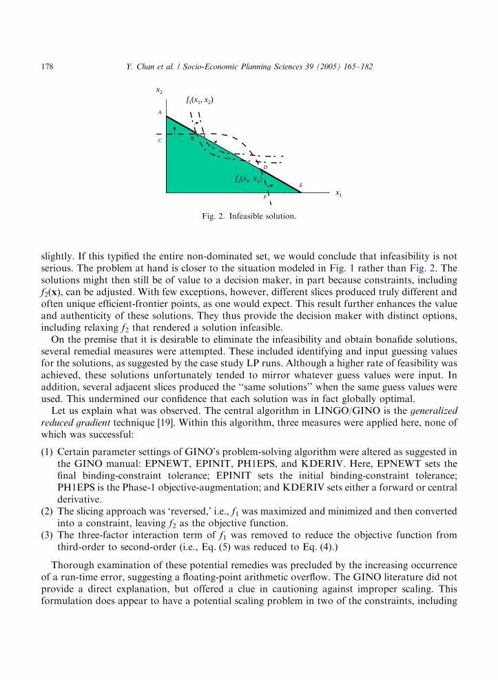
Step 5. Read off each solution as a member of the efficient-frontier set of non-dominatedsolutions.The data set from the case study in Section 5 was used here [18]. All but two of the 50 runs

generated an infeasible solution. Fig. 2 provides a graphical explanation in two dimensions. Thus,while each slice of f2(x) meaningfully defines a feasible region (such as ‘‘wedge’’ PQR) in Fig. 1,f2(x) now dissects it into two disconnected entities—‘‘triangles’’ ABC and DEF in Fig. 2. Thisresults in a non-convex program with an infeasible solution. Notice that such dissection wouldnever occur with a linear objective or criterion function. Here, the two exceptions yielding feasiblesolutions are identical to the linear problem with f1 dominant.Output from the first run was examined in detail to determine the extent of the infeasibility.

Each constraint’s value was computed from the decision variables, with these values compared tothe constraint’s RHS. In so doing, we found only three of the 48 constraints violated, one merely

ARTICLE IN PRESS

x1

x2

f2(x1, x2)

f1(x1, x2)P

Q

R

Fig. 1. Nonlinear implementation of constraint-reduced feasible-region.


slightly. If this typified the entire non-dominated set, we would conclude that infeasibility is notserious. The problem at hand is closer to the situation modeled in Fig. 1 rather than Fig. 2. Thesolutions might then still be of value to a decision maker, in part because constraints, includingf2(x), can be adjusted. With few exceptions, however, different slices produced truly different andoften unique efficient-frontier points, as one would expect. This result further enhances the valueand authenticity of these solutions. They thus provide the decision maker with distinct options,including relaxing f2 that rendered a solution infeasible.On the premise that it is desirable to eliminate the infeasibility and obtain bonafide solutions,

several remedial measures were attempted. These included identifying and input guessing valuesfor the solutions, as suggested by the case study LP runs. Although a higher rate of feasibility wasachieved, these solutions unfortunately tended to mirror whatever guess values were input. Inaddition, several adjacent slices produced the ‘‘same solutions’’ when the same guess values wereused. This undermined our confidence that each solution was in fact globally optimal.Let us explain what was observed. The central algorithm in LINGO/GINO is the generalized

reduced gradient technique [19]. Within this algorithm, three measures were applied here, none ofwhich was successful:

(1) Certain parameter settings of GINO’s problem-solving algorithm were altered as suggested inthe GINO manual: EPNEWT, EPINIT, PH1EPS, and KDERIV. Here, EPNEWT sets thefinal binding-constraint tolerance; EPINIT sets the initial binding-constraint tolerance;PH1EPS is the Phase-1 objective-augmentation; and KDERIV sets either a forward or centralderivative.

(2) The slicing approach was ‘reversed,’ i.e., f1 was maximized and minimized and then convertedinto a constraint, leaving f2 as the objective function.

(3) The three-factor interaction term of f1 was removed to reduce the objective function fromthird-order to second-order (i.e., Eq. (5) was reduced to Eq. (4).)

Thorough examination of these potential remedies was precluded by the increasing occurrenceof a run-time error, suggesting a floating-point arithmetic overflow. The GINO literature did notprovide a direct explanation, but offered a clue in cautioning against improper scaling. Thisformulation does appear to have a potential scaling problem in two of the constraints, including

ARTICLE IN PRESS

x1

x2

f2(x1, x2)

f1(x1, x2)

A

BC

D

E

F

Fig. 2. Infeasible solution.


possible incompatibility between regular constraints and the constraint derived from f1 or f2.Here, coefficient values differed by as much as 103, ranging from 0.005 to 6.29 in one instance, and0.005 to 4.75 in another.In short, our attempt to generalize the linear model failed. While plans were made to renew the

effort at a future date, existing results from the linear model do, indeed, provide meaningfulinsights into the goal-seeking approach to capital budgeting.

7. Conclusion

In this paper, we applied a capital-budgeting model to the problem of technologymodernization in a public organization. It shows how a goal-seeking model addresses a variationof the capital-budgeting problem. This multi-criteria optimization model explicitly considers thediverse functions of the organization. In particular, the synergism amongst the functions ismodeled as a multiplicative value function. The ‘‘constraint reduced feasible-region method’’ isincorporated, resulting in a non-convex mathematical program that produces numericalintricacies. We have seen that even in our relatively simple problem, many hours of effort couldnot produce a solution despite several remedial approaches. Indeed, the additional complexity ofsolving a nonlinear problem may not be worth the extra realism or fidelity in modeling thesituation.Although the goal of solving such a complicated model was not quite achieved in the current

study, we learned much about the process and its inherent challenges. Obviously, a great deal ofthought and careful analysis must precede the formulation of any problem and, in particular, itscriterion functions. Assuming strategic equivalence, we gained a fair amount of insight usinglinearized versions of these criterion functions. To be sure, we cannot always make the convenientassumption of an additive value function. However, linearization of the criterion (objective)functions reduces computational intricacies. An Army-modernization acquisition-study was usedto illustrate the proposed model, showing that its non-inferior solutions are remarkablystable across the different weights one places on diverse missions. This suggests that practicalsolutions can satisfy divergent goals of an organization. Comparison was also made with otherapproaches, typically formulated as goal-setting programs. Most importantly, the modelhighlighted how technology acquisitions are affected as the priorities of each organizationalfunction changes.This multicriteria linear-programming approach has the distinct advantage of employing a

tractable analytic structure, while retaining the essence of the capital-budgeting problem. Forexample, the dual variables here yielded important insights into the modernization plan thatsynergistically supported both missions of interest. Sensitivity analysis readily identifiedincongruity between budgets and requirements—a most useful feature in public organizationswhose budgets are typically subject to public scrutiny. The linear program tended to yield integersolutions, which, again, was advantageous since we were required to acquire integral units of newtechnology. While caution should be used in generalizing this result, the additive linear-programming formulation truly deserves further investigation.In an organization, missions can reinforce one another in achieving macro goals; but a plan can

contribute toward these missions independent of one another. Plans can also support one mission

ARTICLE IN PRESS


while detracting from another. Ideally, acquisition of new technology over time should support allmissions. This way, a modernization plan becomes a critical instrument for the organization toimprove. The study here illustrates how such an objective can be achieved. We showed why it isbetter than setting arbitrary goal-aspiration levels and directly trading off between alternatetechnologies.Admittedly the aggregate, policy-oriented analysis presented here must be ultimately translated

into a detailed acquisition plan. This requires a collateral detailed model similar to those usedelsewhere, including the models reviewed above in the ‘‘Introduction’’ section [2,5]. One couldalso consider maintenance more seriously, which extends service life of existing technologywithout new acquisition [8]. As a public-sector model, learning-curve effects might be modeled torepresent system cost as a function of quantity produced [20], assuming experience helps to refinethe acquisition process. This is particularly important in defense acquisitions, where new weaponsare typically expensive to develop. Uncertainty could also be considered [10]—a useful feature inresearch and development, which is fraught with risks. For the methodologically oriented, a wayto tackle a multiplicative criterion function more novel than what was described above is stillworthy of further investigation.

Acknowledgement and Disclaimer

The authors wish to acknowledge S. Inman and D. Skelton of the US Army Training andDoctrine Command for sponsoring this research. The authors are also grateful for thecontributions of T. Sterle, who performed computation on the nonlinear model. The Editor-in-Chief, Barnett R. Parker, and the two anonymous referees were instrumental in development ofthe manuscript as it went through numerous revisions. The views expressed in this article are thoseof the authors and do not reflect the official policy or position of the Department of Defense orUS Government.

References

[1] Weingartner HM. Mathematical programming and the analysis of capital budgeting problems, Englewood Cliffs,

NJ: Prentice-Hall: 1963.

[2] Brown GG, Clemence RD, Teufert WR, Wood RK. An optimization model for modernizing the Army’s

helicopter fleet. Interfaces 1991;21:39–52.

[3] Loerch A, Koury RR, Maxwell DT. Value added analysis for Army equipment modernization. Naval Research

Logistics 1999;46:233–53.

[4] Jackson J, Kloeber J, Ralston B, Deckro R. Selecting a portfolio of technologies: an application of decision

analysis. Decision Sciences 1999;30(1):217–38.

[5] Coyle RG. The optimization of defense expenditure. European Journal of Operational Research 1992;56:

304–18.

[6] DiSalvo JP. A goal seeking approach to model the injection of future vehicle into the US army inventory. Master’s

thesis, Department of Operational Sciences, Air Force Institute of Technology, Wright-Patterson AFB, Ohio,

1990.

[7] Donahue SF. An optimization model for army planning and programming. Master’s thesis, Department of

Operations Research, Naval Postgraduate School, Monterey, CA, 1992.

ARTICLE IN PRESS


[8] Goodhart CA. Depot-level maintenance planning for Marine Corps ground equipment. Military Operations

Research 1999;4(3):77–89.

[9] Johnson JP. Automatic sensitivity analysis for an army modernization optimization model. Master’s thesis,

Department of Operations Research, Naval Postgraduate School, Monterey, CA 1995.

[10] Meir, H, Christofides, N, Salkin G. Capital budgeting under uncertainty—an integrated approach using

contingent claims analysis and integer programming. Operations Research, 2001;49(2):196–206.

[11] Yoon K. Systems selection by multiple attribute decision making. Doctoral dissertation Department of Industrial

Engineering Kansas State University, Manhattan, Kansas, 1980.

[12] Lee JW, Kim SH. Using analytic network process and goal programming for interdependent information system

project selection. Computers and Operations Research, 2000;27:367–82.

[13] Chan Y. Location theory and decision analysis. Cincinnati, Ohio: Thomson South-Western; 2001.

[14] Keeney RL, Raiffa H. Decisions with multiple objectives: preferences and value tradeoffs. New York: Wiley; 1976.

[15] Zelany M. Multiple criteria decision making. New York: McGraw-Hill; 1982.

[16] Steuer R. Multiple criteria optimization: theory, computation, and application. New York: Wiley; 1986.

[17] Liebman J, Lasdon L, Schrage L, Waren A. Modeling and optimization with GINO. San Francisco, CA: Scientific

Press; 1986.

[18] Sterle T, Chan Y. A multiplicative value function in optimizing acquisition decisions. Working Paper, Department

of Operational Sciences, Air Force Institute of Technology, Wright-Patterson AFB, Ohio, 1994.

[19] Abadie J. The GRG method of nonlinear programming. In: Greenberg HJ, editor. Design and implementation of

optimization software. Alphen a/d Rijn: Sijthoff and Noordhoff; 1978. p. 335–63.

[20] Loerch A. Incorporating learning curve costs in acquisition strategy optimization. Naval Research Logistics

1999;46:255–71.

Yupo Chan is Professor and Founding Chair, Systems Engineering Department, University of Arkansas at Little Rock.

He received his B.S. in civil engineering, M.S. in transportation systems/economics, and Ph.D. in operations research,

all from The Massachusetts Institute of Technology, Cambridge. Professor Chan’s research interests include

telecomunications, transportation, networks and combinatorial optimization, multi-criteria decision-making, spatial–

temporal information, and technology assessment. He has authored or co-authored several books, including Location

Theory and Decision Analysis (ITP/South-Western, 2001) and Location, Transport and Land-use: Modeling Spatial-

Temporal Information (Springer-Verlag, forthcoming). Profesor Chan’s work has appeared in Transportation Planning

and Technology, European Journal of Operational Research, Environment and Planning A, Journal of Urban Planning and

Development, ITE Journal, Transportation Research Record, Military Operations Research, IEEE Transactions in

Reliability, Journal of Engineering Management, Computers & Operations Research, and Journal of Transport

Geography. Dr. Chan is a Fellow of the American Society of Civil Engineers and has won the Harland Bartholomew

Award of the American Society of Civil Engineers, the Koopman Prize of the Operations Research Society of America,

and a Congressional Fellowship with the office of Technology Assessment.

Joseph P. DiSalvo was commissioned in the Armor Corps after graduating from the United States Military Academy,

West Point, NY. He is a graduate of the Armor Officer Basic and Advanced Courses, and the US Army Command and

General Staff College. He earned an M.S. in Operations Research from the Air Force Institute of Technology.

Additionally, he is Airborne and Ranger qualified. His initial assignments were Platoon Leader, Executive Officer, and

Squadron Maintenance Officer in 2d Squadron, 3rd Armored Cavalry Regiment at Ft. Bliss, TX from 1982 to 1985. He

then served in 1st Armored Division in Germany as Battalion Motor Officer; and Commanded A Company and HHC,

2-37 Armor Battalion from 1985 to 1988. From 1990 to 1993, he was an officer systems analyst at US Army PERSCOM

and DA DCSPER. He returned to Germany and had assignments in G3 V Corps; Executive Officer 1-4 Cavalry

Squadron, 3ID; S3 1st Brigade, 3ID; S3 2nd Brigade, 1ID; and Aide-de-Camp to CG, USAREUR from 1994 to 1998.

He then commanded 1st Squadron, 3rd Armored Cavalry Regiment at Ft. Carson, CO from 1998 to 2000. As Colonel,

he is currently based in Carlisle Barracks, PA.

Michael W. Garrambone is Senior Analyst, Veridian Engineering Division, General Dyanmics Corporation, Dayton,

OH. He holds a B.S. in engineering science and mechanics from the University of Florida, Gainesville, an M.S. in

ARTICLE IN PRESS


operations research from the Florida Institute of Technology, Melbourne, and an MBA and M. Education, both from

Georgia State University, Atlanta. Mr. Garrambone has over 30 years of diverse supervisory and analytical experience

in engineering, military modeling and simulation, project management, and economic and decision risk analysis. He has

directed many high-visibility studies employing operations research to solve complex technical, tactical, operational,

and logistical problems.

ARTICLE IN PRESS


Documents

A goal-seeking approach to capital budgeting