1

A GLOBAL OPTIMIZATION ALGORITHM FOR SPACE TRAJECTORY DESIGN

Massimiliano Vasile

European Space & Technology Centre ESA/ESTEC, SERA-A, Keplerlaan 1 2201 AZ Noordwijk,

The Netherlands

Massimiliano.Vasile@esa.int

Abstract

In this paper a combination of Evolution Programming and Branching is used to solve a typical problem in

space trajectory design: finding all possible minimum cost transfers, including the global one, between

two celestial bodies. The idea is to use a limited population evolving for a small number of generations,

according to some specific evolution rules, in subregions of the solution space defined by a branching

procedure. On the other hand the branching rules are functions of the outcome from the local EP

optimization. The proposed combined systematic-heuristic global optimization performs quite well on the

analyzed cases suggesting the possibility of more complex application in space trajectory design.

Introduction A meaningful part of the mission design process consists of designing trajectories. Traditionally this task

has been accomplished using gradient methods, optimal control theory or mathematical tools specifically

dedicated to each particular problem. Anyway all this approaches can be generally classified as local

optimization methods. Since most typical problems are non-convex and may include integer variables or

functions non-differentiable in all the solution space, a significant part of the job is to formulate

appropriately the problem to make it amenable to a solution using local optimization tools and to produce

a reasonably good initial guess1,2. In fact it is likely that the analysts find a local minimum every time they

seek for a solution, eventually finding the global optimum. Furthermore it is often required to find not

simply one optimal solution but all potentially optimal solutions in a given domain.

In this paper a global optimization approach is proposed combining a deterministic method and a

stochastic approach, respectively branching3 and Evolution Programming4,5. This particular combination

2

presents some novel ideas: a migration operator that guides individuals toward promising area of the

solution space, a filter operator (in place of common selection operators) ranking families of potentially

interesting individuals and a particular tunneling technique used to find the global optimum. Moreover EP

is used to obtain lower bound information, to select promising branches and to prune non-promising ones.

Furthermore the algorithm treats both integer and real variables.

The effectiveness of the proposed algorithm is demonstrated on a typical problem in space mission design.

Trajectory Design Problem In an ecliptic reference frame centered into the Sun and considering the gravity action of the Sun only, the

dynamic of a spacecraft is governed by the following differential system:

rv

vr

3rµ−=

=

&

&

(1)

where µ is the gravity constant of the Sun, r is the position vector of the spacecraft and v is its velocity

vector. Now in the hypothesis of Keplerian motion taking two points in space and fixed a time of flight

(TOF) T, Lambert’s problem consists of finding the transfer arc from one point to the other in the given

time. If this is applied to the problem of finding the optimal transfer trajectory from Earth to Mars, an

infinite number of trajectories can be generated, each one characterized by a different departure date from

the Earth t0, a different time of flight T and a different departure velocity ∆vE from the Earth and arrival

velocity ∆vM at Mars. The arrival and departure velocities can be related to the cost in terms of propellant

to transfer a spacecraft from the Earth to Mars, therefore the following objective function can be defined:

ME vvJ 22 ∆+∆= (2)

which must be minimized with respect to the departure time and transfer time.

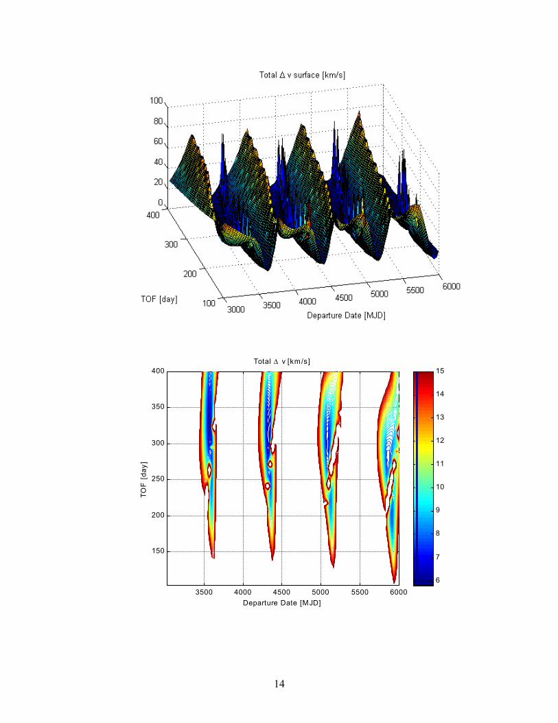
If J is plotted with respect to t0 and T the result can be seen in figures 3 and 4. If an upper limit is imposed

on the maximum total ∆v allowed for an interplanetary mission, the contour plot 4 shows only regions

characterized by a total ∆v lower than the require limit. These regions define what are generally called

launch windows, i.e. intervals of possible launch dates. For the problem under study t0 is defined in the

3

interval [3000, 6000] expressed in Modified Julian Day (i.e. number of days from 1st January 2000) while

the TOF is defined in the interval [100,400] expressed in days. In the given domain D of launch dates and

transfer times, there are at least 8 local minima but actually only one is global with a value of 5.667 km/s.

However a second minimum can be found with a value slightly different 5.699 km/s but for a completely

different launch date.

Optimization Approach The optimization problem can be written as:

Df

∈yy

with )( min

(3)

Proposed optimization approach is composed of an evolution step and a branching step. The evolution

step is meant to obtain information on the possible presence of optima in a subdomain Dl⊆ D. While the

branching step is used to partition the domain D into subdomains Dl.

Evolution Programming The present implementation of evolution programming is based on four fundamental operators: mutation,

migration, mating and filtering. It should be noticed that all of them operates both on real and integer

numbers therefore each individual, represented by a vector y, contains in the first m components integer

values and in the remaining s components real values.

Mutation. Mutation operates in three different ways: generates a random number, taken from a gaussian

distribution, within the domain D or within each subdomain Dl, for each component of y; generates a

symmetric perturbation of a selected component yi with respect to its original value within an interval in a

neighborhood of y; generates an asymmetric perturbation of a selected component yi with respect to its

original value with in an interval in a neighborhood of y.

Migration: migration is a particular mutation of an individual, which generates a micro population in a

neighborhood of y. The best child of the micro population, if better than the parent, is taken as new

principal individual and reproduced in the next generation instead of the parent. If the micro population is

4

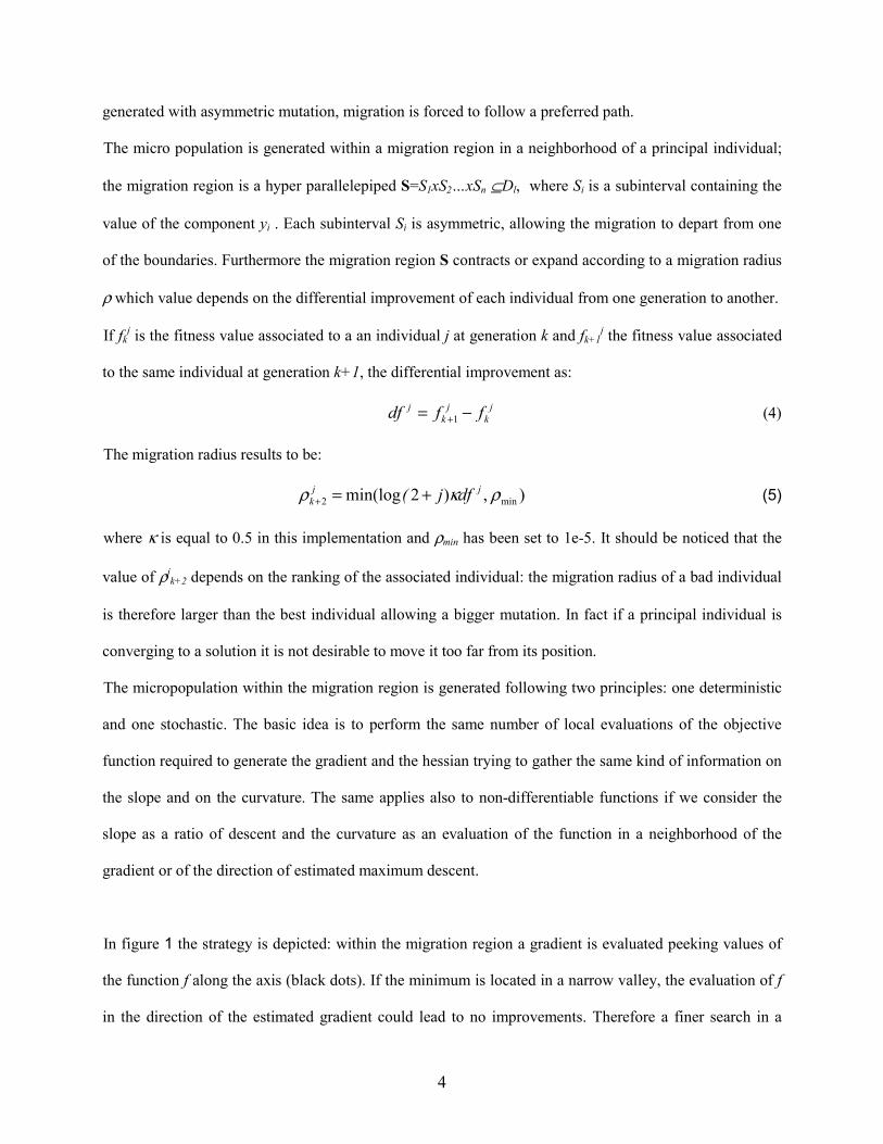
generated with asymmetric mutation, migration is forced to follow a preferred path.

The micro population is generated within a migration region in a neighborhood of a principal individual;

the migration region is a hyper parallelepiped S=S1xS2…xSn ⊆Dl, where Si is a subinterval containing the

value of the component yi . Each subinterval Si is asymmetric, allowing the migration to depart from one

of the boundaries. Furthermore the migration region S contracts or expand according to a migration radius

ρ which value depends on the differential improvement of each individual from one generation to another.

If fkj is the fitness value associated to a an individual j at generation k and fk+1

j the fitness value associated

to the same individual at generation k+1, the differential improvement as:

jk

jk

j ffdf −= +1 (4)

The migration radius results to be:

),)2min(log min2 ρκρ jjk dfj( +=+ (5)

where κ is equal to 0.5 in this implementation and ρmin has been set to 1e-5. It should be noticed that the

value of ρjk+2 depends on the ranking of the associated individual: the migration radius of a bad individual

is therefore larger than the best individual allowing a bigger mutation. In fact if a principal individual is

converging to a solution it is not desirable to move it too far from its position.

The micropopulation within the migration region is generated following two principles: one deterministic

and one stochastic. The basic idea is to perform the same number of local evaluations of the objective

function required to generate the gradient and the hessian trying to gather the same kind of information on

the slope and on the curvature. The same applies also to non-differentiable functions if we consider the

slope as a ratio of descent and the curvature as an evaluation of the function in a neighborhood of the

gradient or of the direction of estimated maximum descent.

In figure 1 the strategy is depicted: within the migration region a gradient is evaluated peeking values of

the function f along the axis (black dots). If the minimum is located in a narrow valley, the evaluation of f

in the direction of the estimated gradient could lead to no improvements. Therefore a finer search in a

5

neighborhood of the gradient and of the other points is performed. Notice that the sub regions overlap to

avoid gaps and systematically unexplored regions.

An evaluation of f is therefore performed along the axis the resulting values are used to compute a search

direction:

mig

mig

xf

p∆∆

= (6)

where ∆fmig is the difference between the individual of the micropopulation and the principal individual

and ∆xmig is the corresponding distance from the principal individual. The length of the deterministic step

is equal to the radius of the hypersphere inscribed into the migration region. After the n+1 deterministic

evaluations a stochastic step follows: a mutation of all n+1 sub individuals is performed in a

neighborhood of the sub individuals generating n individuals for each subindividual. This is equivalent to

evaluate the objective function to build the Hessian. This step is quite computing intensive but can be

reduced if the sparsity pattern of the objective function is available. In fact following the sparsity pattern

for each of the n+1 sub individual only a reduced subset of local evaluations can be done.

The results of a migration is expected to be and individual better than the parent principal individual, if

this is not the case the migration radius is contracted and a new population is generated. Contraction is

given by:

min* ~rρρ = (7)

Where min~r is the minimum distance of the individuals of the subpopulation, with respect to the principal

one, normalized with respect to the dimensions of the migration region.

For integer numbers migration operates in the same way but the migration regions and migration radius

are generated and treated differently. In particular ρimin is 1 and ρ is defined as:

]),)2logmin[int min2 ij

migj

k fj(( ρρ ∆+=+ (8)

The migration region is therefore contracted differently for real and for integer variables allowing a better

6

spatial exploration.

Mating. With a given frequency φ principal individuals are mated following two schemes: exchange of

one randomly chosen component; blending of two correspondent components. In this second case if the i-

th component of two individuals is chosen and a random number α is generated, the resulting child will

have a i-th component given by

123 )1( iii yyy αα −+= (9)

The mating operator is used also to prevent an undesirable effect of migrations: if more than one principal

individual is in the basin of attraction of the same solution it is likely that all of them will move toward the

same point with a resulting waste of resources. Therefore if two or more principal individuals are colliding

(intersecting their migration regions) a repelling mechanism is activated which mates the worse individual

(between two colliding) with the boundaries or the subdomain Dl: According to equation 9, each

component of the selected individual is blended with the value of the furthest bound projecting the

individual into a random point within Dl.

Filtering: instead of traditional selection mechanisms based on fitness here a permanent population of n

individuals is maintained from one generation to another. Each individual has a chance to survive

provided that it remains inside the filter. The filter ranks all the individuals on the base of their fitness

from the best to the worst. All the individuals with fitness lower than a given threshold are completely

mutated while migration is applied to all individuals within the filter. This allows each of the individuals

within the filter to evolve toward a different local optimum. The filter basically operates a simple sorting

procedure but, since individuals in the upper part of the filter are strongly mutated, it is likely that they are

replaced by quite different new individual coming from the associated subpopulation and migration.

In conclusion for the pure EP step two migration is used to explore locally the solution space and two

mechanisms are used for global exploration: mating and mutation of individuals outside the filter. It

7

should be noticed that if several minima are clustered the mixed systematic-stochastic generation of

subpopulation should guarantee anyway to find locally the best minimum of the cluster.

Branching The worst individual coming out from the filter is used to cut the subdomain Dl into q subdomains,

corresponding to q new branches (or nodes). Each node may or may not contain an individual coming

from the previous step of evolution. All empty nodes are rejected and the branching procedure carries on

along branches with a high probability to contain an optima. The probability depends on the fitness of the

individuals belonging to each node and on the ratio between the volume of the associated subdomain Dl

and the number of individuals. i.e. the density of evaluations of the objective function in a given region.

A node with a large number of individuals with high fitness (at the top of the ranking scale) has a high

probability to be explored in the future but the same happens to a node still unexplored. It should be

noticed however that, if the EP have converged in a given subdomain, nodes not containing any

individual, even though they have a large volume, are unlikely to contain the solution. For a fast search,

therefore, only nodes presenting high fitness and large volume are explored further.

In addition the cutting individuals sets an upper bound on the possible value of the objective function

therefore all future individuals with a higher value of the objective function are rejected. For all other

individuals the cutting one works as a repeller forcing a migration toward more promising areas of the

solution space.

Repulsion is performed through a tunneling operator.

Tunneling: In order to increase the chances to find a global optimum a tunneling technique has been

implemented. The basic idea is that all the regions of the solution space below certain fitness are flooded

and all the individuals that want to survive must migrate toward a dry land. The shape of the territory is

changed due to the flooding according to what we called hydrophobic tunneling and the individual, setting

the flooding level, works as a repeller.

8

( )[ ]011ffek −−−= γψ (10)

δβψ

02

rr −= (11)

The process is quite effective to explore the entire solution space in great detail but produces often,

unnecessary reevaluation of many regions where a local minimum has already been found. The result is a

rediscovery of local minima in subdomains getting progressively smaller and smaller with a waste of

computational resources. In order to avoid this phenomenon the original domain is partitioned using more

than one individual. If the worst individual is useful to determine an upper bound on the objective function

and therefore to cut the solution space, converged individuals suggest where a further exploration is

unnecessary.

All converged individuals are ranked depending on the value of their fitness function, the principal cut is

then, as stated above, performed using coordinates of the worst individual, the second cut takes the worst

converged individual and so on up to the best converged individual. A cartoon of the multi-partition

procedure is depicted in figure 2.

Stopping Criterion There are two combined stopping criterions: one for local convergence and one for global convergence.

Both are based on some heuristics and not on any rigorous prove of global converge. Local convergence

of each subpopulation is determined by the differential improvement of the principal individual and by the

migration radius. In a convex problem both should tend to zero in a neighborhood of the solution. Since

each principal individual is supposed either to converge to a different minimum or not to converge (letting

just the individual with highest rank in the filter to converge) a global stopping criterion for the EP is the

convergence of the filter.

The convergence of the filter is determined by the convergence of all the individuals if they are not

clustered, i.e. if their migration regions are not intersecting, and by the convergence of the best individual

9

otherwise. It must be noticed that when EP are used in conjunction with branching the convergence of the

filter is not usually necessary since the branching takes care of the global exploration of the solution

space.

The global convergence of the branching part is based on two ideas: the dimensions of each node and the

convergence of EP in each subdomain. If a node reduces below a given tolerance it is discarded and

considered converged, therefore if no nodes are left, the algorithm stops, on the other hand if EP have

converged in all subdomains and no improvement is reported after branching, i.e. no new local minima are

discovered, the algorithm stops since it is likely that all local minima have been already found and no

further exploration of the solution space is required.

Results Here an example of the results obtained with the combination of EP and branching is reported. At first

only the EP algorithm is tested to verify the effectiveness and efficiency of the new operators. The

problem is solved with no branching step running the EP several times and checking the obtained group of

minima. The stopping criterion in this case is not the complete convergence of the filter but just of the best

individual. A steady population of 10 individuals has been used with a filter containing a maximum of 7

individuals: the individuals outside the filter are therefore strongly mutated. A tolerance of 5e-3 on df and

a tolerance of 1e-3 on the migration radius have been used for the stopping criterion. Since the nature of

the method is stochastic, 20 runs have been performed and the resulting number of function evaluations is

the average of all 20 runs. It should be noticed that only three, out of 20, converged to the second better

minimum without being captured by the basin of attraction of the best minimum. All the others have the

global minimum in the first three positions of the filter and among them, ten have the global minimum as

first value.

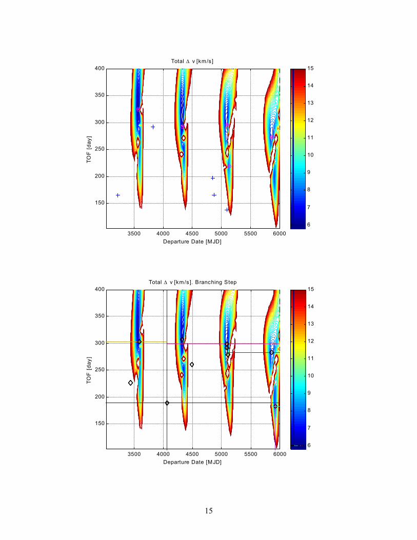
The accuracy of the outcome form the EP step has been verified with an SQP refinement of all the

solutions. An example of a typical run is plotted in Figure 5 and the result is reported in table 1. Notices

that the algorithm successfully found 5 minima (among them the global one in the upper left part of the

10

plot) signed with a fat dot, the other individuals, represented by crosses, are values rejected by the filter. It

is clear form this example that some minima could not be taken into account by the algorithm and among

them there could be the global one especially if, as in this case, more than one minima have similar values

with similar basins of attraction.

The second test includes branching and was used to verify the effectiveness of the branching criterion and

to improve the exploration of the solution space.

The first run of EP spans the entire domain finding a number of minima. Some regions of the solution

space result however unexplored since the choice of the initial population and of regenerated principal

individuals is basically a random process, furthermore it might happen that even though one individual is

initially in the attraction basin of a minimum the filter reject the individual, putting it at the bottom of the

list. This happens especially when some other individuals are close to convergence. Thus some regions

result to be poorly explored because all principal individuals generated do not survive enough to converge

toward a local minimum. Figure 6 reports the result of a branching step from a run of the combined

systematic-stochastic algorithm. The first cutting point is the worst of the individuals rejected by the filter,

this ensures that the resulting branches correspond to either unexplored regions or regions containing

some already found minima. Branches containing converged individuals are correctly partitioned using

these individuals, and the resulting nodes with a high volume and low density as well as branches with

high fitness are evaluated further. After this branching step, however the algorithm stopped declaring

convergence since no improvement was found. Using this technique over other 20 runs, the algorithm was

always able to find the global optimum plus all the other 7 optima. A summary of the obtained minima for

the case represented in Figure 6 is reported in Table 2 where the values found by the evolution branching

algorithm (EPIC) are compared to the values computed refining each solution with a SQP algorithm.

Conclusions In this paper a combined systematic-heuristic approach is proposed to solve trajectory design problems in

which more than one solution is expected and where not just the global optimum should be obtained. The

11

proposed combination of evolution programming and branching is suitable for problems characterized by

differentiable and non-differentiable functions combining integer and real variables. The algorithm is

based only on local information coming from the evolution of a limited number of individuals in

subregions defined by a branching procedure. The outcome of each EP step is used to define new branches

and to prune not promising ones. The particular implementation of evolution programming proposed here

presents some novel operators like migration and filtering that have given quite good results on the

continuous two-dimensional problem under study providing and independent local convergence toward

several local minima. Furthermore the particular mating procedure has demonstrated to be effective to

explore widely the solution space avoiding unnecessary clustering of individuals.

Even though the obtained results and present implementation have to be considered preliminary, the

proposed algorithm appears to be promising even for more complex space trajectory design problems.

References [1] Debban T.J.,McConaghy T.T., Longuski, J.M., Design and Optimization of Low-Thrust Gravity-Assist Trajetories to Selected Planets, AIAA 2002-4729, Astrodynamic Spacialist Conference and Exhibit, 5-8 August 2002, Monterey, California USA. [2]Vasile M. Campagnola S., Bernelli-Zazzera F. Electric Propulsion Options for a Probe to Europa. 2nd International Symposium on Low Thrust Trajectories (LOTUS2), Toulouse 18-20 June 2002. [3] C. Bliek, P.Spellucci, L.N.Vicente, A.Neumaier, L.Granvilliers, E.Huens, P. Van Hentenryck, D. Sam-Haroud, B. Faltings. COCONUT Deliverable D1. Algorithms for Solving Nonlinear Constrained and Optimization Problems: The State of the Art, June 8,2001.The Coconut Project. [4]Michaelewicz Z. Genetic Algorithms + Data Structures = Evolution Programs. Springer- Verlag, Telos, 1996, Third Edition. [5]Vasile M., Comoretto G., Finzi A.E. A Combination of Evolution Programming and SQP for WSB Transfer Optimisation. AIRO2000, September 18-21 2000 Milano, Italy. [6]Barhen J.,Protopopescu V.,Reister D., TRSUT: A Deterministic Algorithm for Global Optimization. Science, 276, 1094-1097 (1997).

12

Table 1. Pure Evolution step with convergence of the best individual

Value Exact Global Optimum Epic Error

J (km/s) 5.667 5.744 1.3%

Departure Date (MJD) 3573.7 3566.0 0.2%

TOF (day) 324.05 325.82 0.3%

Function Evaluations - 476(a) -

(a) Averaged value over 20 runs

Table 2. Summary of minima found by the evolution branching algorithm

Sol. 1 2(b) 3 4 5 6 7 8

SQP 3573.7

324.0

4330.3

306.63

4340.0

252.11

3598.8

276.6

5088.3

295.1

5860.1

277.06

5909.5

201.41

5123.1

221.28

Epic 3573.4

324.1

4332.4

308.85

4347.4

254.93

3599.5

277.58

5084.3

295.5

5864.9

292.58

5909.5

201.82

5125.9

223.5

(b) This solution is a minimum for the subdomain but it is actually in the basin of attraction of sol 1

Figure 1. Criterion for generation of the subpopulation used in migrations

Figure 2. Sketch of the branching procedure

Figure 3 Three-dimensional plot of the total ∆v problem: the objective function is the sum of the ∆v

required to leave the Earth and the ∆v required to insert a spacecraft into Mars orbit.

Figure 4 Contour plot of the total ∆v problem: blue region have low ∆v, red regions have high ∆v while

white areas between two launch windows have excessive cost higher than 15 km/s.

Figure 5 Result from a pure EP step: magenta fat dots are optimal solutions accepted by the filter while

blue crosses are individuals rejected by the filter.

Figure 6 Branching Step

13

Migration Region

Sub region for subindividual generation

Function Evaluation

Worst Individual Worst

converged individual

Best converged individual

14

3500 4000 4500 5000 5500 6000

150

200

250

300

350

400

Departure Date [MJD]

TOF

[da

y]

Total ∆ v [km/s]

6

7

8

9

10

11

12

13

14

15

15

3500 4000 4500 5000 5500 6000

150

200

250

300

350

400

Departure Date [MJD]

TOF

[da

y]

Total ∆ v [km/s]

6

7

8

9

10

11

12

13

14

15

3500 4000 4500 5000 5500 6000

150

200

250

300

350

400

Departure Date [MJD]

TOF

[da

y]

Total ∆ v [km/s]. Branching Step

6

7

8

9

10

11

12

13

14

15