A Geometrically Enhanced Conceptual Model and Query … · pictograms are added to the common ER model to highlight spatial objects and ... [Malinowski and Zim´anyi, ... A Geometrically

A Geometrically Enhanced Conceptual Model and Query

Language

Hui Ma(School of Engineering and Computer Science

Victoria University of Wellington, New [email protected])

Abstract: Motivated by our experiences with spatial modelling for the sustainableland use initiative we present a geometrically enhanced ER model (GERM), whichpreserves the key principles of entity-relationship modelling and at the same timeintroduces bulk constructors and geometric features. The model distinguishes betweena syntactic level of types and an explicit internal level, in which types give rise topolyhedra that are defined by algebraic varieties. It further emphasises the stability ofalgebraic operations by means of a natural modelling algebra that extends the usualBoolean operations on point sets.

Key Words: conceptual model, geometric model, spatial model, entity-relationshipmodel, natural modelling algebra, query language

Category: E.m[Data]:Miscellaneous, H.1.10[Information Systems]:Models and Prin-ciples

1 Introduction

The goal of our research is to provide a conceptual model supporting geometricmodelling. One motivation is the need for spatial data modelling in the contextof the sustainable land use initiative (SLUI) [Mackay, 2007], which addresseserosion problems in the New Zealand hill country. At the core of SLUI wholefarm plans (WFPs) are produced, which capture farm boundaries, paddocks,etc. and provide information about land use capability (LUC) such as rock, soil,slope, erosion, vegetation, plants, poles, etc. Such plans can then be used to getan overview of erosion and vegetation levels and water quality, and to exploitthis information for sustainable land use management.

A number of spatial data models have been proposed in the literature [Gutingand Schneider, 1995; Laurini and Thompson, 1992; Peano, 1890], for a briefsurvey see Section 2. The existing models focus on how to store data and how toefficiently realise storage and operations on such data. However, the purpose ofa conceptual model is to serve as communication tool between domain expertsand information analysts, that abstracts from implementation-level details ofdata storage and data access. Based on our experiences with the modelling ofWFPs we are convinced that more research has to be done to obtain adequateconceptual models supporting geometric modelling. Our objective is to go evenfurther than geographic information systems, and to support other kinds of

Journal of Universal Computer Science, vol. 16, no. 20 (2010), 2986-3015submitted: 7/1/10, accepted: 13/9/10, appeared: 1/11/10 © J.UCS

geometric modelling in the same manner. For instance, technical constructionssuch as rotary piston engines can be supported by trochoids, which are planealgebraic curves already known by the Greeks [Brieskorn and Knorrer, 1981].Bezier curves and patches [Salomon, 2005] are also commonly applied in theseapplications. Together with hull operators [Hartwig, 1996] they can also be usedfor 3-D models of hill shapes in WFPs.

In this paper we introduce the geometrically enhanced entity-relationshipmodel (called GERM for short) as our approach to deal with the problems dis-cussed. As the name suggests, our intent is to preserve the aggregation-basedapproach [Hull and King, 1987] of the original entity-relationship (ER) model bymeans of higher-level relationship types [Thalheim, 2000], but we enhance rolesin relationship types by supporting choice and bulk constructors (sets, lists, mul-tisets). However, different from [Hartmann and Link, 2007] the bulk constructorsare not used to create first-class objects, neither is the choice constructor (defin-ing so-called clusters in [Thalheim, 2000]).

Furthermore, we keep the fundamental distinction between data types suchas points, polygons, Bezier curves, etc. and concepts. The former ones are usedto define the domains of (nested) attributes, while the latter ones are repre-sented by entity and relationship types. That is, a concept such as a paddock isdistinguished from the curve defining its boundary. In this way we guarantee asmooth integration with non-geometric data such as farm ownership, processingand legal information that is also relevant for WFPs, but does not pose a novelmodelling challenge.

GERM has been developed to support modelling at multiple levels. On asyntactic (or surface) level we provide an extendible collection of data types suchas line sequences, polygons, sequences of Bezier curves, or Bezier patches, thathave efficient surface representations. For example, a polygon can be representedby a list of points, and a Bezier curve of order n can be represented by n + 1points – the case n = 2 captures the most commonly known quadratic Beziercurves that are also supported in LATEX.

On an explicit (or internal) level we use a representation by polyhedra[Hartwig, 1996] that are defined by algebraic varieties, i.e., sets of zeros of poly-nomials in n variables. All curves that have a rational parametric representationsuch as Bezier curves [Salomon, 2005], can be brought into such an “implicit”form, e.g. [Gao and Chou, 1992] describes a method for implicitisation based onGrobner bases, and many classical curves that have proven their values in land-care for centuries can be represented in this way [Brieskorn and Knorrer, 1981].This kind of explicit representation bears some similarities to the polynomialmodel of spatial data introduced in [Paredaens and Kuijpers, 1998].

Adequate support for operations on geometric data, such as interiors, unions,or intersections of point sets, defines a third, derived level. To guarantee the

2987Ma H.: A Geometrically Enhanced Conceptual Model ...

geometric stability of these operations we adopt the idea of natural modelling[Hartwig, 1996] and extend it to the data types provided in GERM.

This paper is organised as follows. In Section 2 we give a brief review ofrelated work in the literature. Section 3 assembles some relevant informationon WFPs to set up the context of the study. In Section 4 we introduce theconstituents of GERM emphasising the syntactic level. Section 5 outlines anSQL-based language for expressing queries against GERM conceptual schemas.In Section 6 we discuss the internal representation of geometric data by means ofalgebraic varieties. We illustrate our approach by examples from the modellingof WFPs. Finally, in Section 7 we introduce a natural modelling algebra, anddiscuss its merits with respect to expressiveness and accuracy.

2 Related Work

While there is a lot of sophisticated mathematics around to address geometricmodelling in landcare, and this has a very long tradition as shown in [Brieskornand Knorrer, 1981], spatial and geometric modelling within conceptual modellinghave mainly followed two lines of research – for an overview see [Shekhar andXiong, 2008]. The first one is based on modelling spatial relationships such asdisjointness, touching, overlap, inside, boundary overlap, etc. and functions suchas intersection, union, etc. that are used for spatial primitives such as points,lines, polygons, or regions. Extensions have been proposed to the ER model andto UML class diagrams to support spatial data modelling [Shekhar et al., 1997].However, spatial data types are not considered at the conceptual level. Thanasiset al. [Hadzilacos and Tryfona, 1997] propose the Geo-ER Model that intro-duces special entity sets, relationships, and new constructs to handle propertiesassociated to objects relating to the objects’ position. In [Shekhar et al., 1999]pictograms are added to the common ER model to highlight spatial objects andrelationships. Price et al. [Price et al., 2001] deal in particular with part-whole re-lationships, Ishikawa et al. [Ishikawa and Kitagawa, 2001] apply constraint logicprogramming to deal with these predicates, Gubiani et al. [Gubiani and Mon-tanari, 2008] propose an approach to support the management of consistencyconstraints on multiple representations of the same spatial entity, Malinowskiet al. [Malinowski and Zimanyi, 2007] use spatial integrity constraints to ensurethe semantic equivalence of the conceptual and logical schemas. McKenny etal. [McKenny and Schneider, 2007] handle problems with collections, and Chenet al. [Chen and Zaniolo, 2000] use the predicates in an extension of SQL. In[Shekhar et al., 1999], a set of rules are presented to generate spatial columnsand data types in SQL DDL from entity pictograms. However, the complexityof rules are not discussed and can be very high.

The work in [Behr and Schneider, 2001; Chen and Zaniolo, 2000] links to thesecond line of research expressing the spatial relationships by formulae defined on

2988 Ma H.: A Geometrically Enhanced Conceptual Model ...

point sets applying basic Euclidean geometry or standard linear algebra, respec-tively. Likewise, point sets are used in [Stoffel et al., 2007] to express predicateson mesh of polygons in order to capture motion, and Frank [Frank, 2005] classi-fies spatial algebra operation into local, focal and zonal ones based on whetheronly values of the same location, of a location and its immediate neighbourhood,or of all locations in a zone, respectively, are combined. Christian et al. [Jensenet al., 2004] extend existing algebraic query language to accommodate spatialvalues that exhibit partial containment relationships.

Paredaens and Kuijpers [Paredaens, 1995; Paredaens and Kuijpers, 1998]compare five spatial data models: the raster model [Guting and Schneider, 1995]and the Peano model [Peano, 1890], which represent spatial data by finite pointsets that are either uniformly or non-uniformly distributed over the plane, re-spectively, the Spaghetti model [Laurini and Thompson, 1992] based on contoursdefined as polylines, the polynomial model [Kanellakis et al., 1990; Paredaenset al., 1994] based on formulae that involve equality and inequality of polynomi-als, and the PLA model [Corbett, 1979], which only uses some kind of topologicalinformation without dealing with exact position and shape. While some modelslack theoretical foundations, those that are grounded in theory do not botherabout efficient implementations.

As we can see from above, spatial models discussed in the literature are notsuitable for conceptual modelling of geometric data to provide an abstract viewof the an application domain. Widely used conceptual models like the entity-relationship model and UML do not capture some important semantics inherentin spatial modelling [Shekhar et al., 1999]. Geometric data should be includedinto conceptual models so that it can be conveniently accessed through the sur-face level, while its internal structure is hidden from the user. In the mean time,the conceptual model for geometric data should be closed under geometric setoperations [Schneider, 2009]. Further, the spatial relationships and functions dis-cussed in the literature are in fact derived from underlying representations ofpoint sets, so we need representations on multiple levels as also proposed in [Bal-ley et al., 2004]. Furthermore, when dealing with point sets it is not sufficient todefine spatial relationships and functions in a logical way. We also have to ensure“good nature” in the numerical sense, i.e., the operations must be as accurate aspossible when realised using floating point arithmetics. For example, [Liu et al.,2005] emphasised several spatial conflicts such as determining the accurate spa-tial relationship for a winding road along a winding river as opposed to a roadcrossing a river several times, leading to a classification of line-line relationships.The accuracy problem has motivated a series of modifications to algebras onpoint sets that enhance the standard Boolean operators [Hartwig, 1996] to makethem fit for practical applications of geometric modelling.


3 Whole Farm Plans

As we mentioned this study is motivated by the need for spatial data modellingin the context of the sustainable land use initiative (SLUI). Now let us look inmore detail at the information that should be kept for the SLUI program. Tomanage land in the hill country sustainably, the aim of the SLUI and WholeFarm Plans (WFPs) is to propagate land use change. For the long term theSLUI program has an objective to have 75,000 ha of land improved in the next10 years. To demonstrate the considerable funds being spent are achieving worth-while outcomes, WFPs should be monitored to measure the progress towards theobjective. For example WFP data, including spatial and non-special data, needto be kept to create WFPs and to analyse the effectiveness of the programme,e.g., the upgraded land area.

During the environmental assessment of farms a series of artifacts is gen-erated, including legal titles and parcels maps, paddock maps, land resourceinventories, Land Use Capability (LUC) maps, soil fertility and nutrient maps,pasture production maps, summaries of resource issues, and recommendationsfor the sustainable management of land resources. We are not aiming to illumi-nate every detail of this process, but just want to exemplify the kinds of spatialand non-spatial data that need to be captured in Whole Farm Plans. In doingso we shed some light on the features a conceptual modelling language needs toobserve to be useful for WFP modelling, and for geometric modelling in general.

Paddock maps: Figure 1 contains an example of paddock maps which showsthe boundary of paddocks within a farm. To model the maps we need to considerspatial data as well as non-special data, e.g. an area with paddock code = ‘P01’is defined by its paddock boundary which is a polygon. That is, we need aconceptual model to include Polygon and STRING as abstract data types forpaddock boundaries and paddock codes.

LUC maps: Land resources can be described and evaluated according toLUC classification. The LUC classification has three basic components class,subclass and capability unit. The area under study is divided into landcare unitsby drawing boundaries around areas with similar soil characteristics. A landcareunit polygon represents an area of similar soil characteristics. LUC groups sim-ilar landcare units according to their capacity for sustainable production underarable, pastoral, forestry or conservation uses. The LUC unit (e.g. 3w2) indicatesgeneral capability (classes 1 to 8), the major limitations (4 subclass limitationsof wetness, erosion, soil and climate) and the capability unit (e.g. 2) to link withregional classifications and known best management practices. Figure 2 showsan example of LUC maps. Again to model the information on LUC maps, weneed to consider spatial data, e.g., landcare unit boundaries, and non-spatialdata, e.g. LUC units. For example, an area on the bottom of the map is definedby a polygon and has a value of 3w2 for the LUC unit. For the same value of


Figure 1: An Example of a Paddock Map [AgResearch, 2005]

LUC unit total area can be calculated, e.g. the total area of 3w2 is 20.4 hectares.To demonstrate the improvement of land use capability, LUC maps produced atdifferent years can be compared.

WFP maps: Based on the assessment of land strengths and weaknessesare given by LUC unit, a catalogue of environmental works is recommended.Recommendations for either land use change or management change are basedprimarily on the degree, severity, and location of the soil erosion and the resultanteffects. A set of maps are created to show the locations of planned work. Forexample, as shown in Figure 3, the location of tree planting or fence to be builtare shown on the maps. To model the data on WFP maps, we need to modelthe location information of the planned work, presented as polygons, points orarcs, as well as additional information of the planned work which includes thefinancial support information provided by the regional council.

As we can see from above, WFP data includes classic relational or non-spatialdata (attribute data) such as owner information, investment information, landusability data and spatial data (location data) such as paddock boundaries, LUClandcare unit boundaries, buildings, land and water resources, bridges, tracks,track crossings, enhancement plantings, fences, stone pickings. There is a need tointegrate the spatial and non-spatial data in the SLUI application so that users


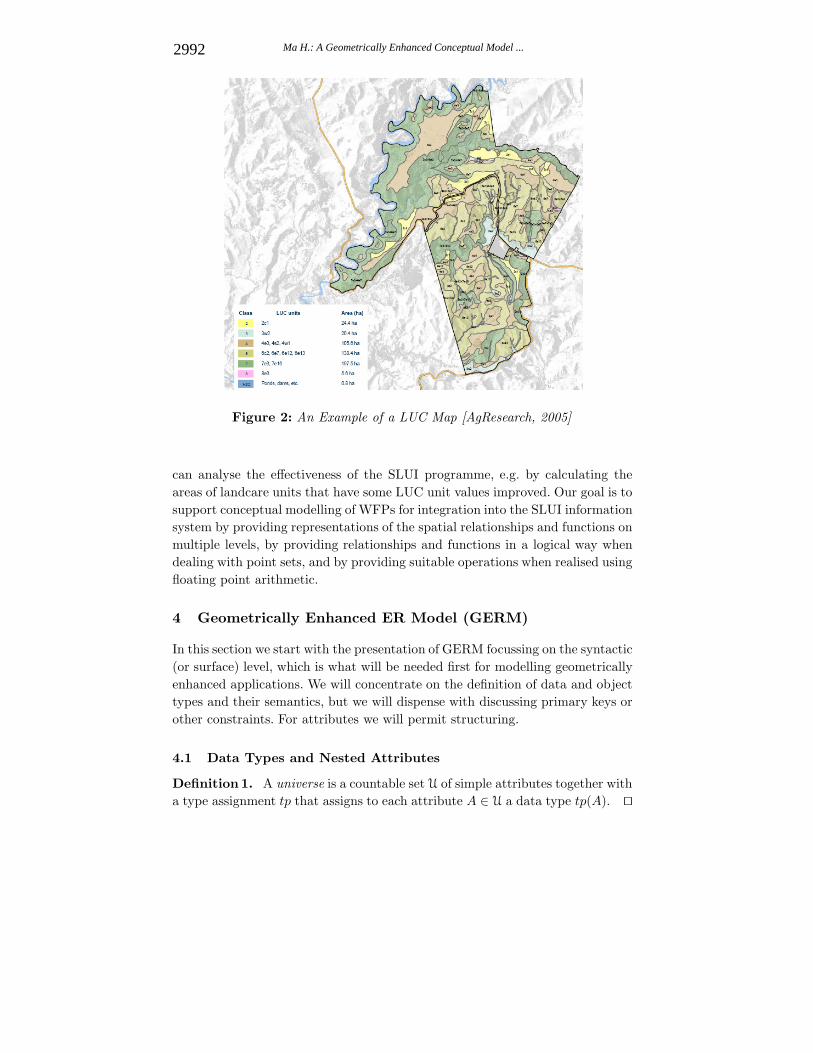
Figure 2: An Example of a LUC Map [AgResearch, 2005]

can analyse the effectiveness of the SLUI programme, e.g. by calculating theareas of landcare units that have some LUC unit values improved. Our goal is tosupport conceptual modelling of WFPs for integration into the SLUI informationsystem by providing representations of the spatial relationships and functions onmultiple levels, by providing relationships and functions in a logical way whendealing with point sets, and by providing suitable operations when realised usingfloating point arithmetic.

4 Geometrically Enhanced ER Model (GERM)

In this section we start with the presentation of GERM focussing on the syntactic(or surface) level, which is what will be needed first for modelling geometricallyenhanced applications. We will concentrate on the definition of data and objecttypes and their semantics, but we will dispense with discussing primary keys orother constraints. For attributes we will permit structuring.

4.1 Data Types and Nested Attributes

Definition 1. A universe is a countable set U of simple attributes together witha type assignment tp that assigns to each attribute A ∈ U a data type tp(A). ��


Figure 3: An Example of a WFP Map [AgResearch, 2005]

For most purposes, the data type tp(A) assigned to an attribute A ∈ U willbe a base type, but we do not enforce such a restriction. We do not further specifythe collection of base types. Common examples of base types are INT , FLOAT ,STRING, DATE , or TIME . Each base type t is associated with a countableset of values dom(t) called the domain of t. For the base types mentioned herethe domains are chosen as usual. For an attribute A ∈ U we let dom(A) =dom(tp(A)), and also call dom(A) the domain of A.

We use constructors to build complex data types from base types. In partic-ular, we use (·) for record types, {·}, [·] and 〈·〉 for finite set, list and multisettypes, respectively, ⊕ for (disjoint) union types, and → for map types. Further-more, we make use of a trivial type 1l with domain dom(1l) = {⊥}. We obtaincomplex data types t by the production rule

t = 1l | b | (a1 : t1, . . . , an : tn) | (a1 : t1) ⊕ · · · ⊕ (an : tn) | {t} | [t] | 〈t〉 | t1 → t2

where b stands for base types, and a1, . . . , an are pairwise distinct labels chosenfrom a suitable alphabet. Moreover, we allow complex data types to be namedand used in type definitions in the same way as base types with the restrictionthat cycles are forbidden. Domains associated with complex data types can beobtained in a similar way from the values of the respective base types and ⊥.

Example 1. We may define named complex data types that can be used forgeometric modelling, such as Point = (x : FLOAT , y : FLOAT) for points in


the two-dimensional plane, PolyLine = [Point ], Polygon = [Point ], Bezier =[Point ], or PolyBezier = [Bezier ]. Note, that the examples PolyLine, Polygon,and Bezier constitute types with identical surface representations, but differentgeometric semantics (details will be discussed in Section 6). A polyline is defineddefined piecewise linearly, while a polygon is a region with a polyline border. ABezier curve is determined by a finite sequence of points in the plane, too. Itpasses through the first and last control points and lies within the convex hull ofthe control points. A polyBezier curve is defined piecewise by Bezier curves. Wewill commonly refer to such data types as geometric data types, thus emphasisingthat they will serve as surface representations for particular geometric features.

The trivial type 1l can be used in combination with the union constructorto define enumerated types, i.e., types with finite domains, such as Bool = (T :1l)⊕ (F : 1l), Gender = (male : 1l)⊕ (female : 1l), or INTn = (1 : 1l)⊕· · ·⊕ (n : 1l)for any positive integer n, which gives a domain with values 1, . . . , n. The mapconstructor can be used to define array types, such as Patch = (i : INTn, j :INTm) → Point representing Bezier patches. Further examples used for spatialmodelling are vector field types of different dimensions, such as Vectorfield1 ={Point} → FLOAT , which is useful for capturing sensor data (e.g., water levels),and Vectorfield2 = {Point} → Point , which is useful for modelling other mea-surements (e.g., wind force and direction) by two-dimensional vectors. Finally,TimeSeries = (d : DATE , t : TIME ) → Vectorfield1 is useful for modelling aseries of observed data over time, thus capturing also temporal aspects of data.

Similar to base types, we may also consider attributes with complexdata types assigned to them. Such attributes are known as nested attributes,cf. [Thalheim, 2000]. We extend this notion as follows:

Definition 2. The set A of (nested) attributes (over universe U) is the smallestset with U ⊆ A satisfying X(A1, . . . , An), X{A}, X [A], X〈A〉, X1(A1) ⊕ · · · ⊕Xn(An), X(A1 → A2) ∈ A with labels X, X1, . . . , Xn and A, A1, . . . , An ∈ A.

��

The type assignment tp extends naturally from U to A as follows:

– tp(X(A1, . . . , An) = (a1 : tp(A1), . . . , an : tp(An)) with labels a1, . . . , an,

– tp(X1(A1) ⊕ · · · ⊕ Xn(An)) = (X1 : tp(A1)) ⊕ · · · ⊕ (Xn : tp(An)),

– tp(X{A}) = {tp(A)}, tp(X [A]) = [tp(A)], tp(X〈A〉) = 〈tp(A)〉, and

– tp(X(A1 → A2)) = tp(A1) → tp(A2).


4.2 Entity and Relationship Types

Following [Thalheim, 2000] the major difference between entity and relationshiptypes is the presence of components ρ : O (with a role name ρ and a name O

of an entity or relationship type) for the latter ones. We will therefore unify thedefinition, and simply talk of object types as opposed to the data types in theprevious subsection. We will, however, permit object types to possess structuredcomponents.

Definition 3. Let O be a countable set of object type names. The set C ofcomponent expressions (over O) is the smallest set containing all object typenames O ∈ O, all list expressions [C], all set expressions {C0}, all multisetexpressions 〈C0〉, and all union expressions C1 ⊕ · · · ⊕ Cn, with C, Ci ∈ C, butwhere the Ci are not union expressions. A structured component is a pair ρ : C

with a role name ρ and a component expression C ∈ C. ��

Note that this definition does neither permit record and map constructors incomponent expressions, nor full orthogonality for set, multiset and union con-structors. We excluded the record constructor as it corresponds to aggregation,i.e. whenever a component of a relationship type has the structure of a record,it can be regarded as a relationship type for its own sake. We decided to excludethe map constructor since functions on entities and relationships that dependon instances seemed to make very little sense to us. The reason the restrictedcombinations of the other constructors are the intrinsic equivalences observedin [Hartmann et al., 2004; Sali and Schewe, 2009]. If in {C} we had a unioncomponent expression C = C1 ⊕ · · · ⊕ Cn, this would be semantically equiva-lent to a record expression ({C1}, . . . , {Cn}), to which the argument regardingrecords can be applied. The same holds for multiset expressions, while nestedunion constructors can be flattened. In this way we guarantee to deal only withnormalised and thus simplified structured components that do not contain anyhidden aggregation.

Definition 4. An object type O of level k ≥ 0 consists of a finite set comp(O) ={ρ1 : C1, . . . , ρn : Cn} of structured components with pairwise different rolenames ρ1, . . . , ρn, and a finite set attr(O) = {A1, . . . , Am} ⊆ A of nested at-tributes. Each object type that occurs in any of the component expressions Ci

is of level at most k − 1, and unless comp(O) = ∅ at least one of these objecttypes must have exactly the level k − 1.

Note that this definition enforces comp(O) = ∅ if and only if O is an objecttype of level 0. Therefore, we call object types of level 0 entity types, and objecttypes of level k > 0 relationship types. For brevity, we use the notation O =(comp(O), attr(O)) to define an object type O. ��


Example 2. Recall that whole farm plans are developed on the basis of pad-dock maps. Each paddock belongs to some farm, is identified by its pad-dock code, is legally defined by a boundary, and has a particular usage.We can use an object type Paddock with structured component farm :Farm and with attributes paddock code, usage, and boundary to model pad-docks. That is, comp(Paddock) = {farm : Farm} and attr(Paddock) ={paddock code, usage, boundary}. Herein, Farm is an entity type and, thus, Pad-

dock is a relationship type of level 1. For simplicity, we agree to omit the rolename (e.g., farm) if it corresponds to the object type name (e.g., Farm) in thecomponent expression.

Note that while we discarded full orthogonality for component constructors,we did not do this for the nested attributes, leaving a lot of latitude to modelers.The rationale behind this flexibility is that the attributes should reflect piecesof information that are meaningful within the application context. For instance,using a simple attribute shape with tp(shape) = Polygon (thus, shape ∈ U)indicates that the structure of polygons as lists of pairs of floating point num-bers is not relevant for the conceptual model of the application, whereas thealternative of having a nested attribute shape([point(x-coord, y-coord)]) withtp(x-coord) = tp(y-coord) = FLOAT would indicate that points and their coor-dinates are conceptually relevant beyond representing a data type. Notice thatthe use of nested attributes in object types also gives rise to a generalised notionof primary keys, which however, is beyond the scope of this paper.

Furthermore, the way we define structured components opens the way forobject types with alternative or collection-type components. For example, onecan define an object type Land Parcel with a set of paddocks as component.However, we do not promote the use of disjoint unions nor sets, lists and multisetsfor first-class concepts. For example, a set of paddocks will not appear as astand-alone object type. This differs from [Thalheim, 2000], where disjoint unions(called clusters) are used independently from relationship types, and also from[Hartmann and Link, 2007], where this has been extended to sets, lists andmultisets. The reason is that such stand-alone constructors are hardly needed inthe model, unless they appear within a component of a object type.

4.3 Schemata and Instances

Finally, we put the definitions of the previous subsections together to defineschemata and their instances in the usual way.

Definition 5. A GERM schema S is a finite set of object types, such thatwhenever ρi : Ci ∈ comp(O) is a structured component of some object typeO ∈ S and the object type name Q appears in Oi, then also Q ∈ S holds. ��


The definition of a GERM schema covers the syntactic level of our conceptualmodel. For the semantics, we need to define instances of a GERM schema. Wewill start with the definition of objects. An interpretation I(O) of an objecttype O is just a finite set of objects of type O. Similar to the extension of dom

from base types to complex data types, we can also extend the interpretationto structured components. This determines a unique set I(Ci) of values for anycomponent expression Ci, which is built from interpretations I(Q) for all Q

appearing in Ci.

Definition 6. An object o of type O is a mapping defined on comp(O)∪attr(O)that assigns to each structured component ρi : Ci ∈ comp(O) a value ci ∈ I(Ci),and to each attribute Aj ∈ attr(O) a value vj ∈ dom(Aj). Objects of an entitytype (i.e., level k = 0) are called entities, while objects of a relationship type(i.e., level k > 0) are called relationships.

For brevity, we use the notation o = (ρ1 : c1, . . . , ρn : cn, A1 : v1, . . . , Am :vm) for an object o of type O = ({ρ1 : C1, . . . , ρn : Cn}, {A1, . . . , Am}). ��

Definition 7. An instance I of a GERM schema S is an S-indexed family{I(O)}O∈S , such that for each object type O ∈ S the set I(O) is an interpreta-tion of O, and only these sets are used to determine the value sets for structuredcomponents. ��

It is common practice to visualise entity-relationship schemas as diagrams.This approach has also been used in the presence of higher-level relationships,see [Thalheim, 2000]. We will adopt this approach to our purposes here, andextend it to include a notation for sets. The GERM diagram of a GERM schemaS is a directed graph with the object types of S as nodes, and with edgesfrom a node O to a node Q whenever Q appears in a structured componentρi : Ci ∈ comp(O). Disjoint unions are indicated by diamonds labelled with ⊕,while sets are indicated by diamonds labelled with ⊗.

Note that the GERM schema and its visualisation as a diagram are justtwo different ways of presenting essentially the same information. We can attachlabels for attributes to the entity or relationship types to increase the level ofdetail. For the sake of readability, however, we have omitted them in Figure 4.For the same reason we have omitted role name labels if they correspond to theobject type name in a structured component.

4.4 An Example: A GERM Schema for WFP Modelling

Example 3. Let us consider a GERM schema for a WFP as illustrated by itsdiagram in Figure 4. Among other it reflects geographic information related withthe farms that are managed with whole farm plans. The central entity type Farm

can have attributes farm name, owner, address, and boundary. The first three


Figure 4: Example of a GERM diagram for WFP modelling

have the base type STRING assigned to them, while tp(boundary) = PolyBezieris the data type assignment for the last one.

The object type Paddock is used to represent the arable land units of afarm (commonly called paddocks), with attributes paddock code, boundary, andusage. The data types assigned to them are STRING, PolyBezier , and (cattle :1l) ⊕ (dairy : 1l) ⊕ (hort : 1l) ⊕ (sheep : 1l) ⊕ · · · ⊕ (other : 1l), respectively.

The object type LUC is used to capture the properties of landcare units ofa farm, with attributes year, boundary, and unit(class, sub class, capability). Weassigned the data types YEAR and PolyBezier to the first two attributes, whilethe third one is a nested attribute formed using a record constructor from theattributes class of data type INT , sub class of data type (w : 1l) ⊕ (e : 1l) ⊕ (s :1l)⊕(c : 1l), and capability of data type INT. Note that the data type of sub classis an enumerated type whose available values indicate wetness, erosion, soil, andclimate (for details please see Section 3 again).

The object type Building is used to represent buildings located on a farm,with attributes base and kind. We assigned a further enumerated type to thenon-spatial attribute kind, and the data type Polygon to the spatial attributebase. The object type Fence has an attribute shape of data type PolyLine, andtwo components: a set of Paddock objects and a set of Path objects, referringto the paddocks and paths it is adjacent to. The object type Path has attributes


width, location, and shape. The latter is of data type PolyBezier , indicating thecourse of the path by a polyBezier curve.

The object types River, Pond and Well are used to model water resourceson a farm. River has attributes river name, location, left and right. The lattertwo are of data type PolyBezier, to capture the course of the left and rightbank of a river. The object type Well possesses attributes well number, depth,and boundary of data types types STRING, FLOAT , and Circle, respectively.The object type Pond has attributes pond name, and boundary of data typesSTRING and PolyBezier , respectively. As usual we may assign different datatypes to attributes (here boundary) if they appear in multiple object types.

The relationship type Inside is used to model part-of relationships that arecommon on a farm. For example, an island may lie in a river, and a well, pondor building may be located in a paddock. Inside has two components, one is adisjoint union of the object types representing parts, while the other is a disjointunion of the object types representing wholes.

A water consent for a farm refers to set of water extraction points, eachof them linked to a water resource (called source) such as a river, a well, ora pond. The object type WaterExtractionPoint has attributes location,capacity, and minimum. The data types assigned to them are Point , FLOAT , andMonth → FLOAT , respectively. capacity specifies the amount of water that maybe taken out of the source, while minimum defines a minimum season-dependentstandard that may not be fallen below. The object type WaterConsent has anattribute allowance of data type Month → FLOAT defining the total amountof water the farm is permitted to use. The object type WaterQuality is usedto model the water quality measured for a water resource (called source) suchas a river or a pond over time. It has a nested attribute measurement{date →reading(agent, unit, value)} to capture measured levels of oxygen, nitrate, orother agents. The object type WasteWaterAgreement is used to model thecontracted minimum and maximum values governing the water quality for afarm.

5 GERM-SQL

Conceptual models are widely used during the analysis and design of data-intensive applications. They provide a high-level documentation of user require-ments, thus facilitate the communication between data architects and domainexperts during requirements capture. As design artifacts they often define a basisfor further development efforts and can be subject to contracts. It is good prac-tice to equip a conceptual modelling language with suitable means for queryingconceptual models. For the entity-relationship model, such as query languageis SQL/ER [Gogolla, 1994] which was created in the spirit of SQL, but omits


some ingredients of classical SQL such as the Group-By-clause. [Abiteboul et al.,1995] introduced O2SQL that extends SQL to cope with complex data. [Thal-heim, 2000] built on the experiences with SQL/ER and O2SQL when suggestingHERM/SQL for the higher-order entity-relationship model. Note, however, thatgeometric data types were not present in HERM, so that HERM/SQL does notprovide adequate support for querying geometric data on the conceptual level.

On the other hand, there is evidence that the use of SQL for certain spa-tial queries is inconvenient and error-prone due to the high syntactic complexity[Lorie and Meier, 1984; Westlake and Kleinschmidt, 1990]. There have been con-siderable efforts to make SQL fit for querying spatial databases, for a summarysee [Schneider, 2009]. Examples include Pictorial SQL [Roussopoulos et al., 1988]and Spatial SQL [Egenhofer, 1994] that extends SQL to cope with spatial dataon the logical level.

In this section we are concerned with the question of how to extendHERM/SQL to cope with geometric data types. The challenge is to equip thequery language with means for describing and composing geometric data thatare compatible with the dual representation of geometric data on the surfaceand the internal level that we use for GERM. Following the extensions of SQLmentioned before, we aim to preserve the Select-From-Where structure of SQLqueries. However, additions are necessary to allow the user to pose queries in-volving geometric features.

Every query Q has GERM schemas Sin and Sout as input and output schema,respectively, and a mapping q that maps instances of Sin to instances of Sout.Unless explicitly specified otherwise, the output schema consists of a single objecttype Ans. Its attributes are given in the Select-clause.

Example 4. The following query asks for the names and boundaries of GoldenKiwi’s farms. Its input schema is the illustrated in Figure 4, its output schemacontains the object type Ans = (∅, {farm name, boundary}).

SELECT farm name, boundaryFROM Farm

WHERE owner = ‘Golden Kiwi’;

The attributes in the Select-clause may be simple or nested attributes. Theymay be already existing attributes of the object types in the input schema,projections thereof to subattributes, or completely new attributes.

Example 5. To analyse the relationship between water quality and land quality,one often want to find out all the farms that have a particular river going through.To following query asks for all those Golden Kiwi farms that have the Manawaturiver going through. Herein, r.vicinity:Farm.farm name denotes the projectionof objects of type River to an attribute of its structured component Farm. In


[Thalheim, 2000] such projections are also denoted using navigation paths in theentity-relationship diagram. For the formal definition of projections on complexdata types using bulk and choice operators, we refer to [Hartmann et al., 2006;Sali and Schewe, 2009].

SELECT r.vicinity:Farm.farm nameFROM River r

WHERE r.river name = ‘Manawatu’ and r.vicinity:Farm.owner =‘Golden Kiwi’;

To provide adequate support for geometric data types, we need to includeoperators acting on the respective domains. Examples are arithmetic operators,such as area for the data types Polygon and Circle, length for the data typesPolyLine, Bezier and PolyBezier, or distance between pairs of points, curves orregions. We further need unary geometric operators, such as closure, interior,and border, and binary geometric operators, such as union, intersection, and dif-ference. A particular challenge that arises here is that the result of applying suchoperators does not necessarily belong to the same domain anymore. We discussthis issue in more detail in Section 7. Moreover, we may also use aggregationfunctions, such as average, minimum, and sum.

Example 6. The following query asks for the overall size of Golden Kiwi’s farms.

SELECT sum(area(boundary)) as total landFROM Farm

WHERE owner = ‘Golden Kiwi’;

In the Where-clause we may also use Boolean operators, in particular thosereflecting topological relationships between points, curves and regions, such ascontains, covers, meets, or disjoint. Finally, the structure of queries may beextended by further clauses as known from classical SQL, e.g., the Group-By-clause.

Example 7. As part of the Sustainable Land Use Initiative (SLUI), the landquality of participating farms is inspected on an annual basis. The outcomesof this inspection are modelled by the object type LUC. A summary of theoutcomes for a particular year according to the LUC classification can beretrieved using the following query.

SELECT �.unit(class, sub class, capability), sum(area(�.boundary))FROM LUC �

WHERE �.in:Farm.farm name = ‘Rainbow Farm’ and �.in:Farm.year = 2009GROUP BY �.unit(class, sub class, capability);


The previous query can easily be extended to retrieve the improvement in landquality over a certain period:


WHERE �.in:Farm.farm name = ‘Rainbow Farm’ and �.in:Farm.year = 2009GROUP BY �.unit(class, sub class, capability);MINUS


WHERE �.in:Farm.farm name = ‘Rainbow Farm’ and �.in:Farm.year = 2005GROUP BY �.unit(class, sub class, capability);

6 Geometric Types and Algebraic Varieties

Usually, the domain dom(t) associated with a data type t defines a set of valuesand a set operations acting on these values. For geometric data, however, thisapproach needs to be questioned. For example, a value of data type Bezier asdefined in the previous section is simply a list of n + 1 points p0, . . . ,pn ∈ R

2.However, it defines a Bezier curve of order n in the two-dimensional plane.This calls for an additional geometric domain gdom(t), which associates with ageometric data type t a suitable set of point sets in the n-dimensional Euclideanspace R

n, together with a mapping dom(t) → gdom(t). In the following we willconcentrate on the case n = 2, i.e., we focus on points, curves and regions inthe plane, but most definitions are not bound to this restriction. We will usealgebraic varieties and polyhedra to define the point sets of interest.

Definition 8. An (algebraic) variety V of dimension n is the set of zeroes of apolynomial P in n variables, i.e., V = {(x1, . . . , xn) ∈ R

n | P (x1, . . . , xn) = 0}.A base polyhedron H is the intersection of half planes, i.e.,

H = {(x1, . . . , xn) ∈ Rn | Pi(x1, . . . , xn) ≥ 0 for i = 1, . . . , k}

where P1, . . . , Pk are polynomials in n variables. A polyhedron H is the union ofa finite set of base polyhedra H1, . . . , H�. ��

It is well-known that algebraic varieties in the plane include all classical two-dimensional curves [Brieskorn and Knorrer, 1981]. Note that P (x1, . . . , xn) = 0holds if and only if both P (x1, . . . , xn) ≥ 0 and −P (x1, . . . , xn) ≥ 0 hold true,so base polyhedra are straightforward generalisations of algebraic varieties.

If a point set is defined by polynomials as in Definition 8, this is calledan implicit representation of the point set. Alternatively, point sets are oftengiven by a function γ(u) : R → R

n which is called an explicit or parametric


representation of the point set [Gao and Chou, 1992]. Note that an parametricrepresentation can always be turned into an implicit one, while the converse isnot always possible. For most two-dimensional point sets of interest, however, itis possible to find rational parametric representations [Gao and Chou, 1992].

Example 8. Take the simple example of the unit circle. It has the implicit repre-sentation P (x, y) = x2 + y2 = 0, but also the rational parametric representation

γ(u) = (x, y) with x =2u

u2 + 1and y =

1 − u2

1 + u2.

Example 9. A Bezier curve of degree n is defined by n + 1 control points

p0, . . . ,pn. A parametric representation is B(u) =n∑

i=0

Bin(u) · pi (0 ≤ u ≤ 1).

Herein Bin denotes the ith Bernstein polynomial of degree n, which is defined as

Bin(u) =(

n

i

)ui(1 − u)n−i.

A Bezier curve of degree 1 is simply a straight line between its two controlpoints p0 and p1. A Bezier curve of degree 2 is a parabolic curve connectingp0 with p2 such that its tangents in both points pass through p1. To obtainan implicit representation for it, we can start with the two quadratic equationsx = au2 + bu + c and y = du2 + eu + f that define B(u) = (x, y). Dividingthese equations by a and d, respectively, and subtracting them from each othereliminates the quadratic term u2. This can then be solved to give u, pluggedback in to give x and y leading to a polynomial in x and y of degree 2 thatdefines the implicitisation of the Bezier curve.

Example 10. A Bezier patch is defined by an (n×m) array of control points pij .

A parametric representation is P (u, v) =n∑

i=0

m∑j=0

Bin(u) · Bjm(v) · pij . If we fix

u = 0 or v = 0, we obtain Bezier curves P (0, v) and P (u, 0), respectively.

Definition 9. The geometric domain gdom(t) associated with a geometric datatype t is a set of point sets. Each element of gdom(t) has an implicit represen-tation by a polyhedron H = H1 ∪ · · · ∪H� with base polyhedra Hi (i = 1, . . . , �)defined by polynomials Pi1, . . . , Pini . For each of the polynomials Pij , the al-gebraic variety defined by Pij has an explicit parametric representation γij(u),unless this is impossible. ��

To obtain suitable polyhedra for two-dimensional regions surrounded by poly-gons or polyBezier curves one often triangulates the region first. Triangulationsare a popular topic in computational geometry, and a number of algorithms havebeen proposed in the literature to find triangulations efficiently.

Note that the union and the intersection of two polyhedra are polyhedraagain, but this is not generally true for their difference. Polyhedra are always


closed sets with respect to the standard topology on the Euclidean space Rn, but

the difference of closed sets is not necessarily closed. We may, however, regaina polyhedron by building its closure. For a geometric domain, it desirable to

have operators available to obtain the closure X , interior◦X, and the boundary

∂X of a point set X in the geometric domain. The semantics of these operators

can be defined in the usual way by◦X = {p ∈ X | ∃r > 0.Ur(p) ⊆ X},

∂X = {p | ∀r > 0.Ur(p) ∩ X �= ∅ �= Ur(p) − X}, and X = X ∪ ∂X . Herein,Ur(p) denotes the open set of radius r > 0 with centre p in the Euclidean spaceR

n.

7 Mathematical Challenges in 2D Geometric Modelling

Let us concentrate on geometric data types whose associated geometric domainsconsist of two-dimensional polyhedra. The polynomials P needed to define two-dimensional polyhedron give rise to plane algebraic curves. The association ofgeometric domains to geometric data types in GERM unlocks the wealth of awide range of (partly very old) mathematical results that are ready for exploita-tion in conceptual modelling of geometric data.

7.1 Logical Properties

Paredaens and Kuijpers [Paredaens and Kuijpers, 1998] studied semi-algebraicsets from the point of view of generic database queries. Typical geometric querieswould involve semi-algebraic sets A, their interior A, boundary ∂A, closure A

and complement R−A, distances, angles, and also spatial relations as mentionedin the introduction.

The key question addressed in [Paredaens and Kuijpers, 1998] is complete-ness. In the context of relational databases, a query language is complete if itcan express all computable queries, i.e., all queries that can be expressed by apartial recursive function that is generic in the sense that it commutes with allisomorphisms. Isomorphisms for relational databases are defined by permuta-tions acting on the domain of values, which are then extended to tuples andrelations in a canonical way.

This approach, however, cannot be transferred to geometrical queries withoutmaking changes to the notion of isomorphism, as arbitrary permutation of pointsin Euclidean space would destroy all geometric properties. Therefore, genericityhas been defined with respect to various groups that operate on Euclidean spacesuch as the group T of translations and the group I of isometries, i.e. transfor-mations that preserve distances. Unfortunately, for many relevant groups G theproperty of G-genericity is undecidable [Paredaens et al., 1994]. Still, Gyssens etal. [Gyssens et al., 1997] were able to define languages that capture exactly theG-generic queries for some relevant groups such as T and I.


Each such transformation group G expresses the geometric properties wewould like to preserve in queries, so the completeness results in [Gyssens et al.,1997] show that for the most relevant cases we can adequately query databasesinvolving geometric objects that are defined by semi-algebraic sets, i.e. we obtainagain semi-algebraic sets as the result of such queries. Furthermore, the executionplans of such queries prescribe the level of accuracy that will be required forelementary operations on point sets such as union and intersection.

7.2 Classification of Plane Algebraic Curves

While querying can be effectively expressed, we want to go further and demandthat one must also be able to retrieve a surface representation by means ofgeometric data types in GERM. For that, we require translations from polyhedrato the domain values of a geometric data type t, that is, a mapping from gdom(t)back to dom(t).

For this let us take a closer look at plane algebraic curves, that is, algebraicvarieties defined by polynomials with two variables. In order to understand howto approach operations on these objects (and thus the polyhedra defined bythem), we may exploit the classification of such curves, for which we considerthe degree of the defining polynomial P . If the degree of P is 1, we have P (x, y) =ax+by+c with coefficients a, b, c ∈ R. Obviously, polynomials of degree 1 defineall straight lines in the plane, including the degenerated case of a single point.If the degree of P is 2, we have P (x, y) = ax2 + by2 + cxy + dx + ey + f

with coefficients a, b, c, d, e, f ∈ R. It is known that polynomials of degree 2define all cone sections [Brieskorn and Knorrer, 1981], that is, all circles, ellipses,parabolas, and hyperbolas, including the degenerated cases of straight lines, twostraight lines and a single point.

For a semi-algebraic set A defined by formula ϕ we can then apply de Mor-gan’s laws to obtain a form, in which negation only appears in front of atomicformulae. From the fact that ¬P (x, y) ≥ 0 is equivalent to P (x, y) < 0 andfurther to −P (x, y) > 0 we can further eliminate negation completely for theprice of permitting > in our formulae. Using laws of distributivity we can furtherarrange A as a union of intersections of elementary semi-algebraic sets that aredefined by P (x, y) ≥ 0 or P (x, y) > 0. As emphasised in [Ma et al., 2009] mostapplications of geometric modelling deal with compact sets, i.e., we are mainlyinterested in elementary sets defined by P (x, y) ≥ 0. The intersection of suchsets will then be defined by sections of plane algebraic curves.

Thus returning to the cases of degree 1 and 2, the result of the most relevantoperations union, intersection and difference (modulo boundaries) gives rise toregions with boundaries defined piecewise by straight lines and cone sections.This is in accordance with the geometric data types provided by GERM. Inparticular, Bezier curves are sections of parabolas.


Furthermore, as non-degenerated cone sections are smooth, we always ob-tain an explicit parametric representation as discussed in Examples 8 and 9 forcircles and parabolas, respectively, and this enables us to easily obtain the pa-rameterisation of sections. If C(u) is a parameterisation of a subsection of a conesection with parameter u ∈ [0, 1], and C(u0) and C(u1) (for u0 < u1) defines asubsection of this curve, then this subsection can be obtained by a simple linearparameter transformation, i.e., C′(u) = C((u1 − u0) · u + u0) for 0 ≤ u ≤ 1defines the parameterisation of the subsection.

Similarly, the case of degree 3 requires the discussion of the following fourcases [Brieskorn and Knorrer, 1981]:

xy2 + ey = ax3 + bx2 + cx + d (1)

xy = ax3 + bx2 + cx + d (2)

y2 = ax3 + bx2 + cx + d (3)

y = ax3 + bx2 + cx + d (4)

These equations have already been carefully analysed by Newton using adetailed investigation of 78 cases. Some of these curves were already knownby the ancient Greeks, e.g., the kissoid of Diocles, the folium Cartesii and theNeilean parabola defined by the polynomials y2(2r − x)− x3, x3 + y3 + axy, andx3 − y2, respectively.

Note that in the case of degree 3, curves can observe singularities, but nev-ertheless can be composed piecewise by smooth sections. For these sections weobtain parametric representations, which give rise to explicit parameterisationsof their subsections.

7.3 Natural Modelling Algebra

The two layers of GERM support the storage and retrieval of geometric objectswithin a conceptual model. The challenge is, however, the manipulation of suchobjects by queries and transactions. For this we now present an algebra ongeometric objects. As we always have an internal representation by point sets,we first focus on these.

Standard operations on point sets are of course the Boolean ones, i.e. union,intersection, difference, and complement. In combination with interior, closureand boundary these operations are in principle sufficient to express a lot ofrelationships between the geometric objects as discussed widely in the conceptualGIS literature (see e.g. [Behr and Schneider, 2001; Shekhar and Xiong, 2008]).For instance, A − B = ∅ is equivalent to A ⊆ B, so we only need difference and

an emptiness test. Similarly,◦A ∩ B = ∅ ∧ ∂A ∩ ∂B �= ∅ express that A and B

touch each other, but do not intersect.


However, relying on the Boolean set operations is insufficient. We have toaddress two concerns: 1) The closure problem: The set of point sets of interestmust be closed under the operations. For example applying the operations onpolyhedra should also return a polyhedra. We already remarked at the end ofthe previous section that this is not true for the set difference and complementoperation. 2) The stability problem: The operations must be numerically stableso that unavoidable numerical error, which are due to the rounding that is nec-essary when dealing with floating-point representations of real numbers, remainsbounded and very small and that no large errors occur.

We can circumvent the closure problem as we are merely interested in pointsets “up to their boundary”. That is, we will apply an equivalence relation ∼where A ∼ B holds for two geometric if and only if A = B. Then each equivalenceclass has exactly one closed representative: a polyhedron. The problem then isthat the Boolean operations do not preserve this equivalence, and we lose someof the properties of a Boolean algebra. However, these properties are volatileanyway due to the necessary modifications that we propose to deal with thestability problem.

For the stability problem, some conceptual modelling experts might arguethat this concerns only an implementation. We do not share this opinion as anyresult obtained by operations of point sets (i.e. the polyhedra on the internallevel) must be re-interpreted by a value of the respective geometric data typeon the surface level. For instance, the union and intersection of polygons mustagain be represented as a polygon, having a finite sequence of points as its surfacerepresentation. Furthermore, we must be aware that the intersection of two two-dimensional curves may be more than just a discrete set of points when thestability problem is addressed adequately. Thus, stability considerations have annon-negligible impact on the surface level of GERM.

7.4 Modification of Boolean Operations

It is known that Boolean operations on point sets may be instable. For instance,for two straight lines their intersection point may be only obtainable with anintolerable error. This problem occurs, when the angle between the two lines isvery small. Our solution will replace the intersection operation by a modifiedoperation, which in this case will enlarge the result. Thus, we actually obtain apoint set instead of a single point. The enlargement will depend on the operands,so that for the uncritical cases we almost preserve the Boolean operations.

In general, we use the following new operations on point sets: A � B =A∪B∪q(A, B) and A ∩+ B = (A∩B)∪q(A, B) with a natural modelling functionq that assigns a point set to a pair of point sets. The name “natural modelling”is adopted from [Hartwig, 1996], as it should reflect properties associated withstability and the original union and intersections operations in a natural way.


We do not modify the complement X ′ of a set X . With A ∪- B = (A′ ∩+ B′)′ andA ∩- B = (A′ � B′)′ we obtain two more modified operations. The simple ideabehind these operations is to slightly enlarge (or reduce) unions and intersectionsin order to cope with the stability problem. The enlargement (or reduction)depends on the arguments; critical operands require larger modifications thanuncritical ones.

Definition 10. A function q from pairs of point sets to point sets is called anatural modelling function iff it satisfies the following properties for all A, B:

q(A, B) = q(B, A) q(A′, B) = q(A, B) q(A, ∅) = ∅

��

We require q to be symmetric, as the stability problem for building inter-sections and unions does not depend on the order. Analogously, the potentialinstability caused by A and B is the same as the one caused by A′ and B.

The simple idea behind these operations is to slightly enlarge unions andintersections in order to cope with the accuracy problem. The enlargement de-pends on the arguments – critical operands require larger modifications thanuncritical ones.

Definition 11. The natural modelling algebra consists of the set of equivalenceclasses of polyhedra with respect to ∼ and the operations �, ∩+ , ∩- and ∪- witha natural modelling function q. ��

Hartwig [Hartwig, 1996] studied the algebraic properties of the direct mod-elling algebra (P(E),�, ∩+ ) and the small modelling algebra (P(E),�, ∩- ). Inboth cases we obtain a weak Boolean algebra, i.e., the existence of neutral andinverse elements is preserved, and the de Morgan laws still hold, but other prop-erties of Boolean algebras have been abandoned.

Using the idea of a “natural modelling algebra” an intersection point of twocurves may be replaced by several points. In doing so, the desirable property ofhaving the exact intersection is given up in favour to a “global” minimisationof error. For instance, if the union of two regions requires the computation ofan intersection point pi of two curves γ1 and γ2, then the approach may resultin two points q and r instead, and instead of building subsections of γ1 andγ2 involving the point pi we may get subsections involving the point q or r,respectively, and the straight line between q and r will be added to the solution.

7.5 Computing with Polyhedra and Surface Representations

The key question is of course how to choose a good natural modelling func-tion q. Before addressing this let us first look at the modified operations on


polyhedra. As these are defined by algebraic varieties, it will be decisive (andsufficient) to understand the operations on two half-planes A = {(x1, . . . , xn) |P (x1, . . . , xn) ≥ 0} and B = {(x1, . . . , xn) | Q(x1, . . . , xn) ≥ 0}. If A and B areplane curves, we have to compute their intersection point(s) in order to deter-mine a surface representation of their union and intersection, respectively. Letus discuss this further for polygons and regions defined by a sequence of Beziercurves.

��

��

��

��•D

•E

•F��

��

•A

•B

•C•H•K

��

��

��

•A•B

•C

•E

•G •F

•D •H

•K

Figure 5: On the left the intersection of two polygons, on the right the intersectionof two regions with a boundary defined by Bezier curves

Example 11. Let us look at the union / intersection of two polygons depicted onthe left in Figure 5, one defined by the points A, B, C, the other one by D, E, F .With A = (1, 1), B = (3, 4), C = (7, 2), D = (3, 0), E = (7, 4), and F = (9, 1)the line through D and E is defined by P (x, y) = x − y − 3 = 0, and the linethrough B and C is defined by Q(x, y) = x + 2y − 11 = 0. They intersect inthe point H = (5.66, 2.66). This intersection divides the plane into four partsdepending on whether P (x, y) and Q(x, y) take positive or negative values.

If we can compute the intersection points H and K, then A, B, H, E, F, D, K

defines the surface representation of the union, while K, H, C defines the one ofthe intersection.

However, the angle between the lines DE and AC at the intersection pointK is rather small, which may cause a different result defined by the operations �and ∩- instead of ∪ and ∩, respectively. The resulting polygon for the modifiedunion may become A, B, H, E, F, D, K1, K2, while the resulting polygon for themodified intersection may become K ′

1, H, C, K ′2 with points K1, K2, K

′1, K

′2 in a

small neighbourhood of K.At H the angle between the two intersecting lines is nearly a right angle, so

the modified intersection may coincide with the normal one.

Example 12. Look at the two regions defined on the right in Figure 5,both defined by values of the data type PolyBezier , the first one by[(A, B), (B, E, C), (C, A)], the second one by [(D, B, F ), (F, G), (G, D)]. As inthe previous example the two intersection points H and K of the line (A, C)


with the Bezier curve (D, E, F ) are decisive for the computation of the unionand intersection.

With A = (16, 5), B = (22, 4), E = (20, 3), C = (21, 0), D = (13, 4),F = (19, 0), and G = (13, 0) the parametric representation of the Beziercurve can be easily obtained as B(u) = (−12u2 + 18u + 13,−4u2 + 4),and the straight line gives rise to x + y − 21 = 0. SubstitutingB(u) = (x, y) in this gives rise to a quadratic equation with the

roots u1/2 =9 ±√

1716

, i.e. u1 = 0.304 and u2 = 0.82, which define

H = (17.32, 3.64) and K = (19.69, 1.31). Then the union can be representedby [(A, B), (B, E, C), (C, K), (K, F ′, F ), (F, G), (G, D), (D, D′, H), (H, A)]of the data type PolyBezier , while the intersection is represented by[(H, H ′, K), (K, H)]. Once H and K are known, it is no problem to ob-tain the necessary points D′ and H ′, as sections of Bezier curves are againBezier curves.

As in Example 11 the computation of the point K canbe expected to be relatively stable, whereas H is not. Us-ing � instead of the usual union, we end up with a modifiedunion represented by [(A, B), (B, E, C), (C, K), (K, F ′, F ), (F, G),(G, D), (D, D′, H1), (H1, H2), (H2, A)] of the data type PolyBezier , whereH1 and H2 are points in the vicinity of H on the Bezier curve and the straightline (H, A), respectively. Analogously, using ∩- instead of ∩, we obtain arepresentation [(H ′

2, H′1)(H

′1, H

′, K), (K, H ′2)] with points H ′

1, H′2 in the vicinity

of H on the Bezier curve and the straight line (H, K), respectively.

7.6 The Choice of the Natural Modelling Function

In view of the discussion in the previous subsection it is sufficient to considerbase polyhedra, i.e. if H = H1 ∪ · · · ∪ Hn and H ′ are polyhedra, we define

q(H, H ′) =n⋃

i=1

q(Hi, H′). Furthermore, for base polyhedra it is sufficient to

consider the boundary, i.e. if H and H ′ are base polyhedra, we define q(H, H ′) =q(∂H, ∂H ′). In the two-dimensional plane E = R

2 we can therefore concentrateon plane curves. If such a curve γ is defined by a union of (sections of) algebraic

varieties, say V1 ∪ · · · ∪ Vn, then we define again q(γ, γ′) =n⋃

i=1

q(Vi, γ′). If q is

symmetric, the naturalness conditions in Definition 10 are obviously satisfied.In order to obtain a good choice for the natural modelling function q it

is therefore sufficient to look at two curves γ1 and γ2 defined by polynomialsP (x, y) = 0 and Q(x, y) = 0, respectively. Let p1, . . . ,pn be the intersectionpoints of these curves – unless γ1 = γ2 we can assume that there are only finitelymany. Then we define q(γ1, γ2) =

⋃ni=1 Ui with neighbourhood Ui = Uγ1,γ2(pi)

as defined next.


Definition 12. For ε > 0 the ε-band of a variety V = {(x, y) | P (x, y) = 0} isthe point set Bε(V ) = {(x′, y′) | ∃(x, y) ∈ V.|x − x′| < ε ∧ |y − y′| < ε}. ��

8 Conclusion

In this paper we presented the geometrically enhanced ER model (GERM) as ourapproach to conceptual geometric modelling. GERM preserves aggregation asthe primary abstraction mechanism of the entity-relationship model, but loosensthe definition of relationship types permitting bulk and choice constructors to beused for components without first-class status of bulk objects. Geometric featuresin the application domain can be modelled by attributes that have geometricdata types assigned to them. This defines a syntactic level of GERM that largelyremains within the popular ER framework and thus enables a smooth integrationwith non-geometric modelling. It also allows users to cope with modelling tasksthat involve geometry in a familiar, non-challenging way thereby preserving allthe positive experience made with entity-relationship modelling.

The syntactic level is complemented by an internal level that employs alge-braic varieties, i.e., sets of zeros of polynomials, to represent geometric featuresas point sets. The use of such varieties leads to a significant increase in expres-siveness way beyond standard approaches that mostly support points, lines andpolygons. In particular, common shapes such as circles, ellipses, or Bezier curvesand patches are captured in a natural way. However, for polynomials of highdegrees we have to face computational problems.

The highly expressive internal level of GERM makes geometric modelling notonly very flexible, it is only the basis for an extended algebra that generalisesand extends the standard Boolean operators on point sets. By using this algebra,GERM enables a higher degree of accuracy for derived geometric relationships.

Our next short-term goal is to apply GERM to WFP modelling for theSustainable Land Use Initiative (SLUI). In order to support the wider objectivesof this programme, GERM is general enough to capture spatio-temporal data aswell. We are also looking for applications beyond GIS. On the theoretical side weplan to investigate further back and forth translations between the syntactic andthe internal level of GERM, and special cases of the natural modelling algebrafor specific applications. In this sense this paper is only the start of a largerresearch programme devoted to geometric conceptual modelling.

Achnowledgement

I am grateful to my former colleagues at the Horizons Council for discussions.


References

[Abiteboul et al., 1995] Abiteboul, S., Hull, R., and Vianu, V. (1995). Founda-tions of Databases. Addison-Wesley.

[AgResearch, 2005] AgResearch (2005). Farm plan prototype for SLUI. re-trieved online from the New Zealand Association of Resource Managementhttp://www.nzarm.org.nz/KinrossWholeFarmPlan A4 200dpi secure.pdf.

[Balley et al., 2004] Balley, S., Parent, C., and Spaccapietra, S. (2004). Mod-elling geographic data with multiple representations. International Journal ofGeographical Information Science, 18(4):327–352.

[Behr and Schneider, 2001] Behr, T. and Schneider, M. (2001). Topological re-lationships of complex points and complex regions. In Conceptual Modeling –ER, volume 2224 of LNCS, pages 56–69. Springer.

[Brieskorn and Knorrer, 1981] Brieskorn, E. and Knorrer, H. (1981). Plane Al-gebraic Curves. Birkhauser.

[Chen and Zaniolo, 2000] Chen, C. X. and Zaniolo, C. (2000). SQLST : A spatio-temporal data model and query language. In Conceptual Modeling – ER 2000,volume 1920 of LNCS, pages 96–111. Springer.

[Corbett, 1979] Corbett, J. P. (1979). Topological principles in cartography.Technical paper 48, US Bureau of the Census.

[Egenhofer, 1994] Egenhofer, M. J. (1994). Spatial sql: A query and presentationlanguage. IEEE Transactions on Knowledge and Data Engineering, 6:86–95.

[Frank, 2005] Frank, A. U. (2005). Map algebra extended with functors for tem-poral data. In Perspectives in Conceptual Modeling – ER Workshops, volume3770 of LNCS, pages 194–207. Springer.

[Gao and Chou, 1992] Gao, X. S. and Chou, S. C. (1992). Implicitization ofrational parametric equations. Journal of Symbolic Computation, 14:459–470.

[Gogolla, 1994] Gogolla, M. (1994). Extended Entity-Relationship Model: Fun-damentals and Pragmatics. Springer.

[Gubiani and Montanari, 2008] Gubiani, D. and Montanari, A. (2008). A con-ceptual spatial model supporting topologically-consistent multiple representa-tions. In International Conference on Advances in Geographic Information Sys-tems – GIS, pages 1–10. ACM.

[Guting and Schneider, 1995] Guting, R. H. and Schneider, M. (1995). Realm-based spatial data types: The ROSE algebra. VLDB J., 4:243–286.


[Gyssens et al., 1997] Gyssens, M., Van den Bussche, J., and Van Gucht, D.(1997). Complete geometrical query languages. In PoDS, pages 62–67. ACM.

[Hadzilacos and Tryfona, 1997] Hadzilacos, T. and Tryfona, N. (1997). An ex-tended entity-relationship model for geographic applications. SIGMOD Record,26(3):24–29.

[Hartmann and Link, 2007] Hartmann, S. and Link, S. (2007). Collection typeconstructors in entity-relationship modeling. In Parent, C. et al., editors, Con-ceptual Modeling – ER, volume 4801 of LNCS, pages 307–322. Springer.

[Hartmann et al., 2004] Hartmann, S., Link, S., and Schewe, K.-D. (2004).Weak functional dependencies in higher-order datamodels. In FoIKS, volume2942 of LNCS, pages 116–133. Springer.

[Hartmann et al., 2006] Hartmann, S., Link, S., and Schewe, K.-D. (2006). Ax-iomatisations of functional dependencies in the presence of records, lists, setsand multisets. Theor. Comput. Sci., 355(2):167–196.

[Hartwig, 1996] Hartwig, A. (1996). Algebraic 3-D Modeling. A. K. Peters.

[Hull and King, 1987] Hull, R. and King, R. (1987). Semantic database mod-eling: Survey, applications, and research issues. ACM Computing Surveys,19(3):201–260.

[Ishikawa and Kitagawa, 2001] Ishikawa, Y. and Kitagawa, H. (2001). Sourcedescription-based approach for the modeling of spatial information integration.In Conceptual Modeling – ER, volume 2224 of LNCS, pages 41–55. Springer.

[Jensen et al., 2004] Jensen, C. S., Kligys, A., Pedersen, T. B., and Timko, I.(2004). Multidimensional data modeling for location-based services. VLDB J.,13(1):1–21.

[Kanellakis et al., 1990] Kanellakis, P., Kuper, G., and Revesz, P. (1990). Con-straint query languages. In PoDS, pages 299–313. ACM.

[Laurini and Thompson, 1992] Laurini, R. and Thompson, D. (1992). Funda-mentals of Spatial Information Systems. Academic Press.

[Liu et al., 2005] Liu, W., Chen, J., Zhao, R., and Cheng, T. (2005). A refinedline-line spatial relationship model for spatial conflict detection. In Perspectivesin Conceptual Modeling – ER Workshops, volume 3770 of LNCS, pages 239–248.Springer.

[Lorie and Meier, 1984] Lorie, R. and Meier, A. (1984). Using relational DBMSfor geographical databases. GeoProcess., 2:243–257.


[Ma et al., 2009] Ma, H., Schewe, K.-D., and Thalheim, B. (2009). Geometri-cally enhanced conceptual modelling. In Conceptual Modeling – ER, volume5829 of LNCS, pages 219–233. Springer.

[Mackay, 2007] Mackay, A. (2007). Specifications of whole farm plans as a toolfor affecting land use change to reduce risk to extreme climatic events. AgRe-search.

[Malinowski and Zimanyi, 2007] Malinowski, E. and Zimanyi, E. (2007). Logicalrepresentation of a conceptual model for spatial data warehouses. Geoinformat-ica, 11(4):431–457.

[McKenny and Schneider, 2007] McKenny, M. and Schneider, M. (2007). PLRpartitions: A conceptual model of maps. In Advances in Conceptual Modeling–ER Workshops, volume 4802 of LNCS, pages 368–377. Springer.

[Paredaens, 1995] Paredaens, J. (1995). Spatial databases, the final frontier. InGottlob, G. and Vardi, M. Y., editors, ICDT, volume 893 of LNCS, pages 14–32.Springer.

[Paredaens and Kuijpers, 1998] Paredaens, J. and Kuijpers, B. (1998). Datamodels and query languages for spatial databases. Data and Knowledge Engi-neering, 25(1-2):29–53.

[Paredaens et al., 1994] Paredaens, J., Van den Bussche, J., and Van Gucht, D.(1994). Towards a theory of spatial database queries. In PoDS, pages 279–288.ACM.

[Peano, 1890] Peano, G. (1890). Sur une courbe qui remplit toute une aire plane.Mathematishe Annalen, 36:157–160.

[Price et al., 2001] Price, R., Tryfona, N., and Jensen, C. S. (2001). Modelingtopological constraints in spatial part-whole relationships. In Conceptual Mod-eling – ER, volume 2224 of LNCS, pages 27–40. Springer.

[Roussopoulos et al., 1988] Roussopoulos, N., Faloutsos, C., and Sellis, T. K.(1988). An efficient pictorial database system for PSQL. IEEE Trans. Soft-ware Eng., 14(5):639–650.

[Sali and Schewe, 2009] Sali, A. and Schewe, K.-D. (2009). A characterisation ofcoincidence ideals for complex values. Journal of Universal Computer Science,15(1):304–354.

[Salomon, 2005] Salomon, D. (2005). Curves and Surfaces for Computer Graph-ics. Springer.


[Schneider, 2009] Schneider, M. (2009). Spatial and spatio-temporal data mod-els and languages. In Encyclopedia of Database Systems, pages 2681–2685.Springer.

[Shekhar et al., 1997] Shekhar, S., Coyle, M., D.-R. Liu, B. G., and Sarkar, S.(1997). Data models in geographic information systems. Communications of theACM, 40(4):103–111.

[Shekhar et al., 1999] Shekhar, S., Vatsavai, R. R., Chawla, S., and Burk, T. E.(1999). Spatial pictogram enhanced conceptual data models and their transla-tion to logical data models. In Agouris, P. and Stefanidis, A., editors, IntegratedSpatial Databases, Digital Images and GIS, volume 1737 of LNCS, pages 77–104.Springer.

[Shekhar and Xiong, 2008] Shekhar, S. and Xiong, H., editors (2008). Encyclo-pedia of GIS. Springer.

[Stoffel et al., 2007] Stoffel, E.-P., Lorenz, B., and Ohlbach, H.-J. (2007). To-wards a semantic spatial model for pedestrian indoor navigation. In Advancesin Conceptual Modeling – ER Workshops, volume 4802 of LNCS, pages 328–337.Springer.

[Thalheim, 2000] Thalheim, B. (2000). Entity Relationship Modeling – Founda-tions of Database Technology. Springer.

[Westlake and Kleinschmidt, 1990] Westlake, A. and Kleinschmidt, I. (1990).The implementation of area and membership retrievals in point geography usingsql. IEEE Data Eng. Bull., 13(3):4–11.


Documents

A Geometrically Enhanced Conceptual Model and Query … · pictograms are added to the common ER model to highlight spatial objects and ... [Malinowski and Zim´anyi, ... A Geometrically