Embed Size (px)
Citation preview
Machine LearningA Geometric Approach
Professor Liang Huang
Linear Classification:Support Vector Machines (SVM)
some slides from Alex Smola (CMU)
CIML book Chap 7.7
Linear Separator
SpamHam
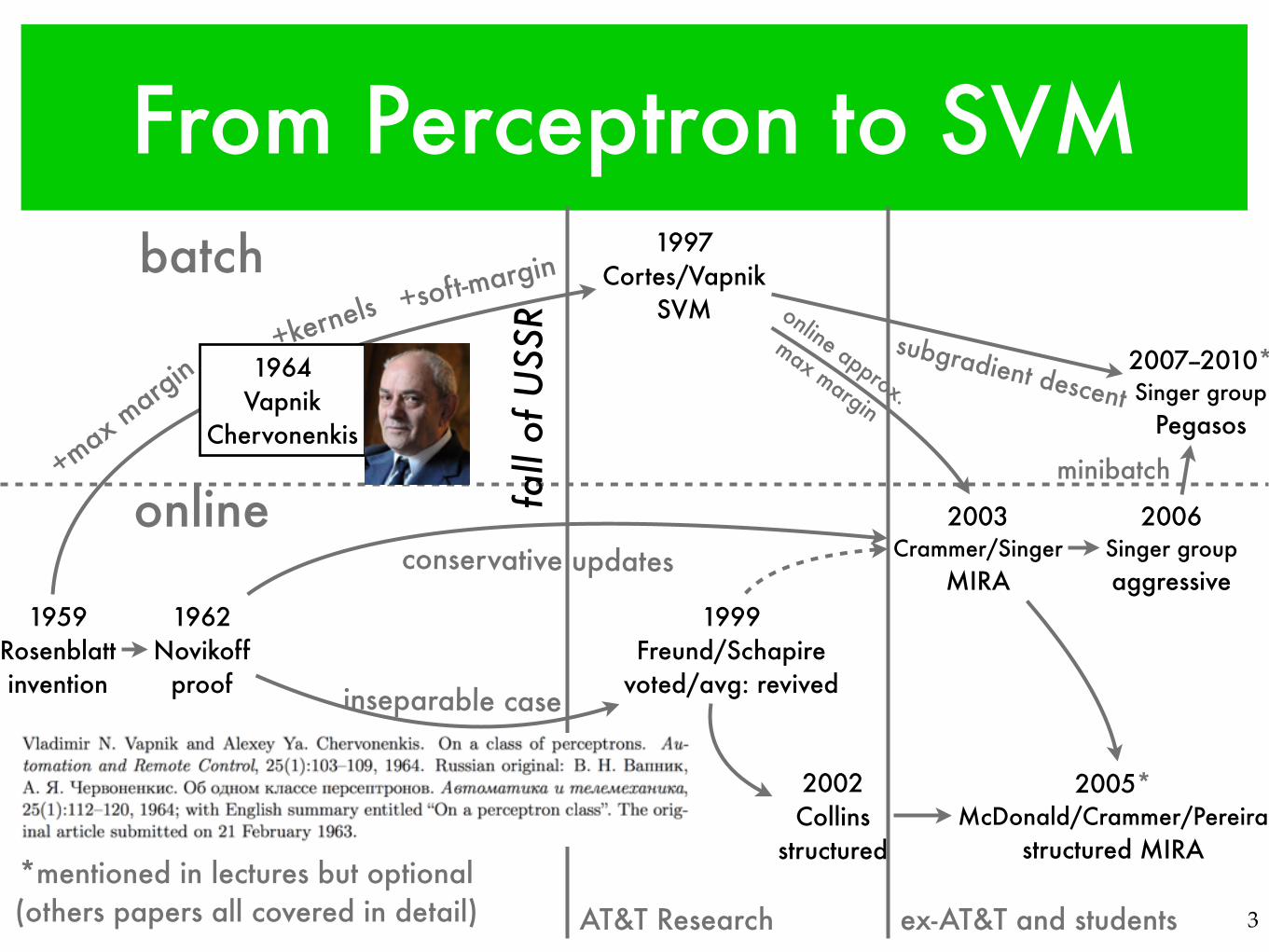
From Perceptron to SVM
1959Rosenblattinvention
1962Novikoff
proof
1999Freund/Schapire
voted/avg: revived
2002Collins
structured
2003Crammer/Singer
MIRA
1997Cortes/Vapnik
SVM
2006Singer groupaggressive
2005*McDonald/Crammer/Pereira
structured MIRA*mentioned in lectures but optional(others papers all covered in detail)
online approx.
max margin
+max margin
+kernels +soft-margin
conservative updates
inseparable case
2007--2010*Singer group
Pegasos
subgradient descent
minibatch
batch
online
AT&T Research ex-AT&T and students
1964Vapnik
Chervonenkis
fall
of U
SSR
3

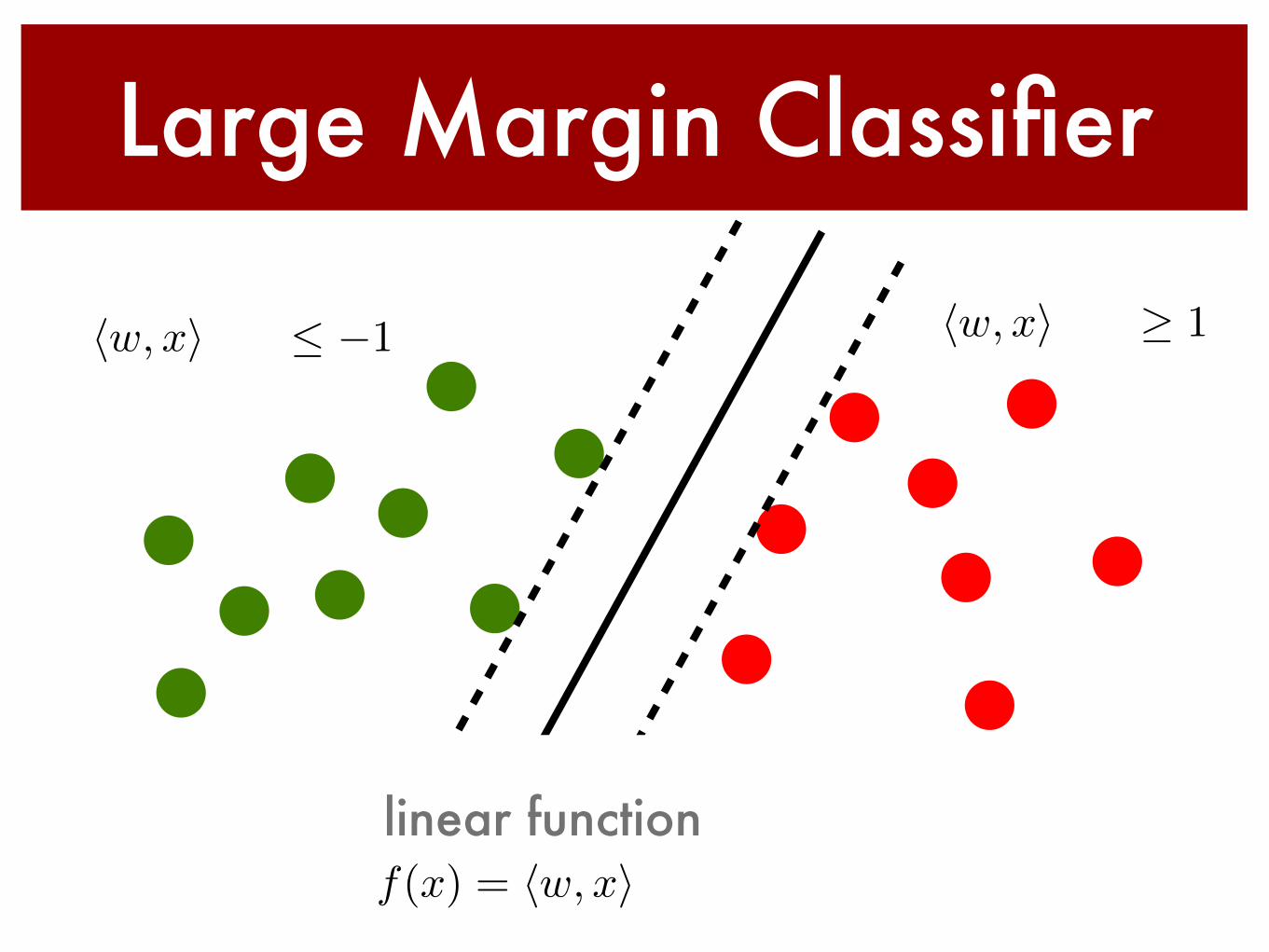
Large Margin Classifier
hw, xi+ b �1 hw, xi+ b � 1
f(x) = hw, xi+ b
linear function
Large Margin Classifier
f(x) = hw, xi+ b
linear function
hw, xi+ b � 1hw, xi+ b �1
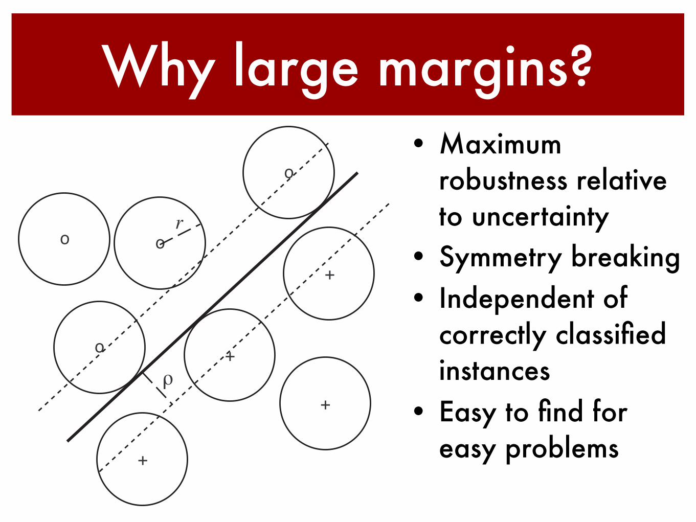
Why large margins?• Maximum
robustness relative to uncertainty
• Symmetry breaking• Independent of
correctly classified instances
• Easy to find for easy problems
Scholkopf and Smola: Learning with Kernels — Confidential draft, please do not circulate — 2012/01/14 15:35
7.2 The Role of the Margin 201
∆x ∈ H is bounded in norm by some r > 0. Clearly, if we manage to separate thetraining set with a margin ρ > r, we will correctly classify all test points: Since alltraining points have a distance of at least ρ to the hyperplane, the test patternswill still be on the correct side (Figure 7.3, cf. also [146]).
o
o
o
+
+
+
o+
r
ρ
Figure 7.3 Two-dimensional toy example of a classification problem: Separate ‘o’ from‘+’ using a hyperplane. Suppose that we add bounded noise to each pattern. If the optimalmargin hyperplane has margin ρ, and the noise is bounded by r < ρ, then the hyperplanewill correctly separate even the noisy patterns. Conversely, if we ran the perceptronalgorithm (which finds some separating hyperplane, but not necessarily the optimal one)on the noisy data, then we would recover the optimal hyperplane in the limit r → ρ.
If we knew ρ beforehand, then this could actually be turned into an optimalmargin classifier training algorithm, as follows. If we use an r which is slightlysmaller than ρ, then even the patterns with added noise will be separable with anonzero margin. In this case, the standard perceptron algorithm can be shown toconverge.1
1. Rosenblatt’s perceptron algorithm [423] is one of the simplest conceivable iterativeprocedures for computing a separating hyperplane. In its simplest form, it proceeds asfollows. We start with an arbitrary weight vector w0. At step n ∈ N, we consider thetraining example (xn, yn). If it is classified correctly using the current weight vector (i.e.,if sgn ⟨xn,wn−1⟩ = yn), we set wn := wn−1; otherwise, we set wn := wn−1+ηyixi (here,η > 0 is a learning rate). We thus loop over all patterns repeatedly, until we can completeone full pass through the training set without a single error. The resulting weight vectorwill thus classify all points correctly. Novikoff [369] proved that this procedure terminates,provided that the training set is separable with a nonzero margin.
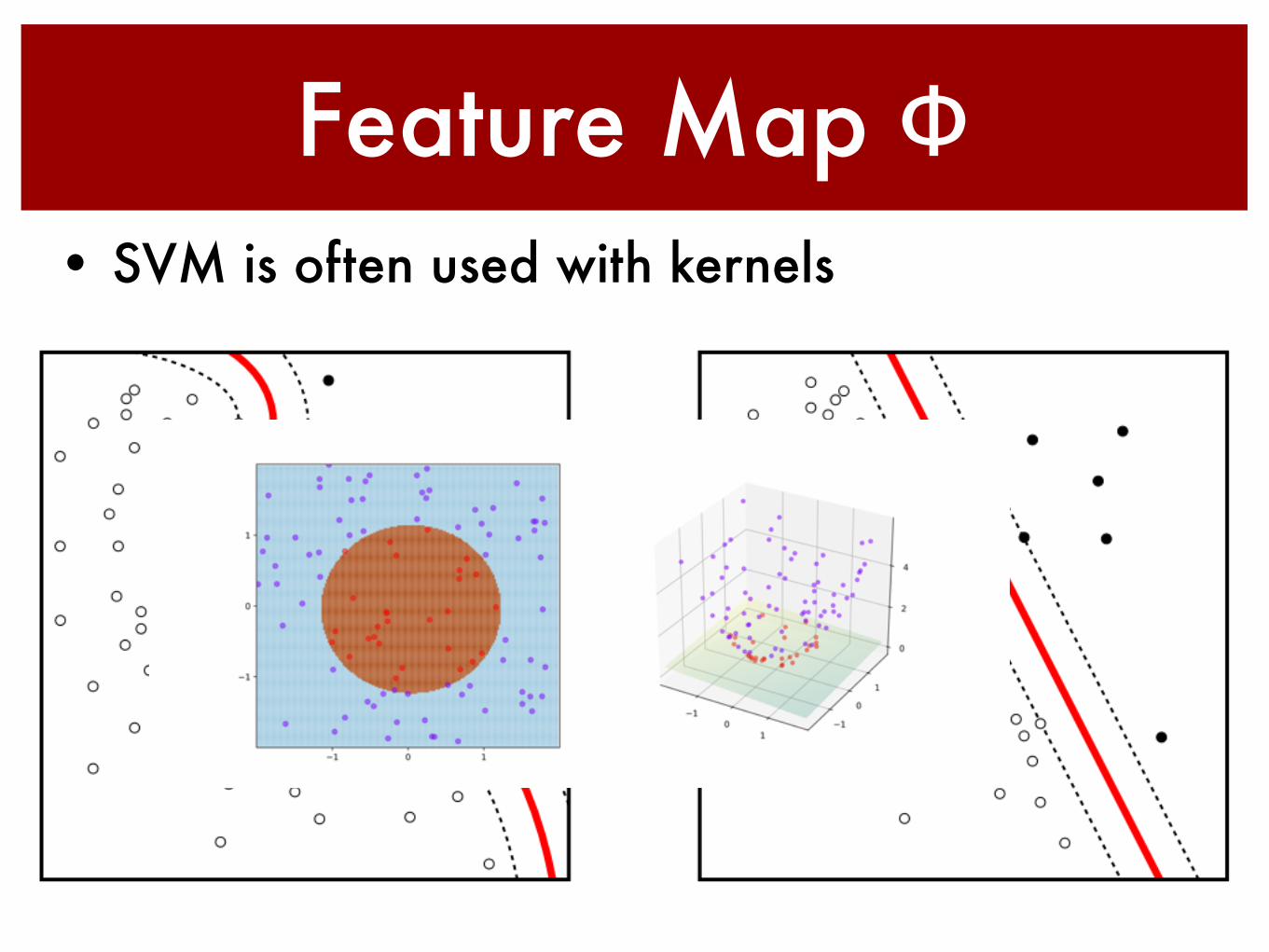
Feature Map Φ• SVM is often used with kernels
hw,
x
i+b
=�1
hw,
x
i+b
=1
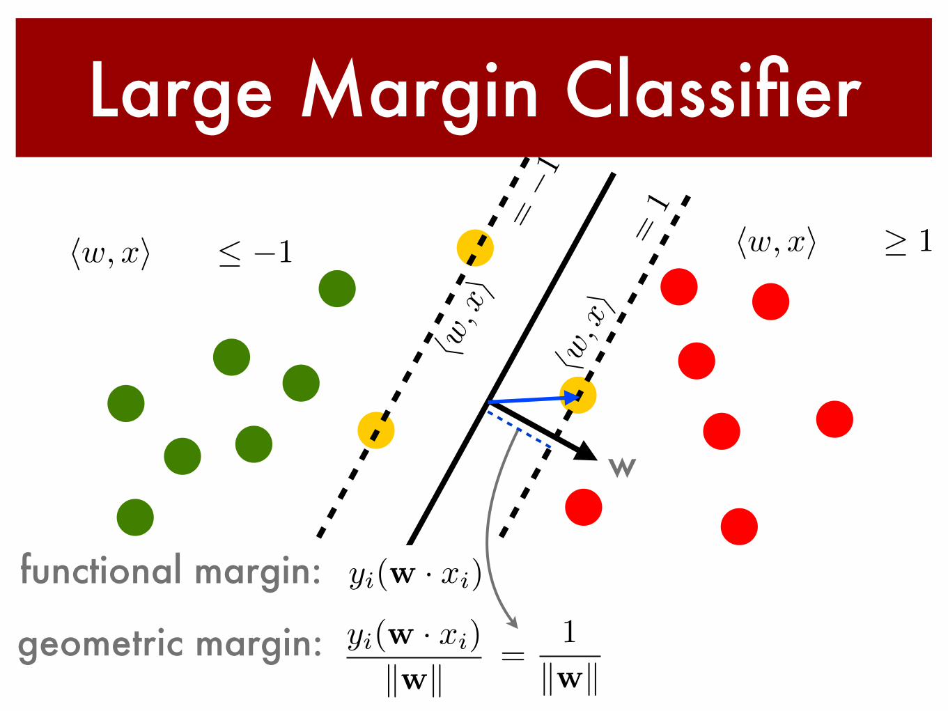
Large Margin Classifier
geometric margin:
w
hw, xi+ b � 1hw, xi+ b �1
functional margin: yi(w · xi)
yi(w · xi)
kwk=
1
kwk
hw,
x
i+b
=�1
hw,
x
i+b
=1
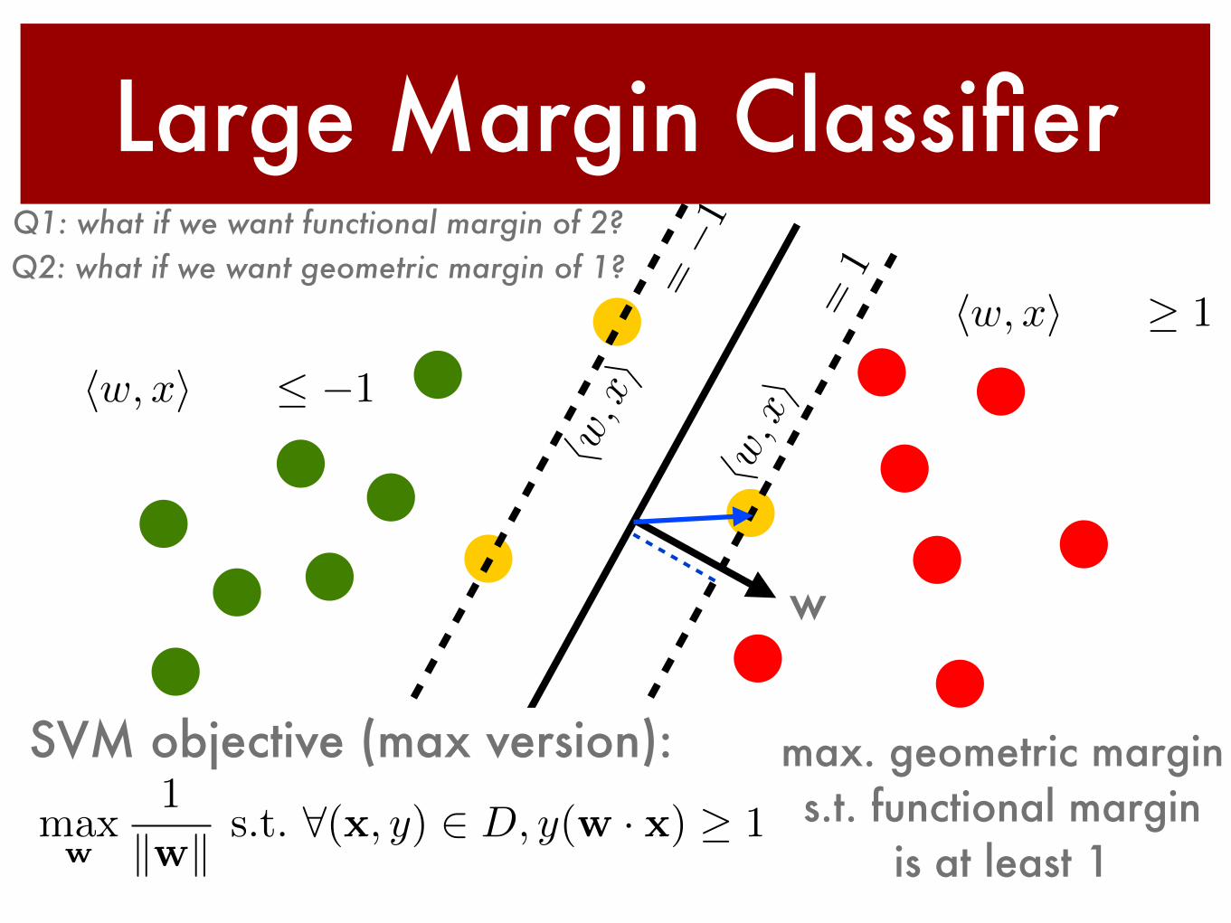
Large Margin Classifier
max. geometric margin s.t. functional margin
is at least 1
w
hw, xi+ b � 1
hw, xi+ b �1
SVM objective (max version):max
w
1
kwk s.t. 8(x, y) 2 D, y(w · x) � 1
Q1: what if we want functional margin of 2?Q2: what if we want geometric margin of 1?
hw,
x
i+b
=�1
hw,
x
i+b
=1
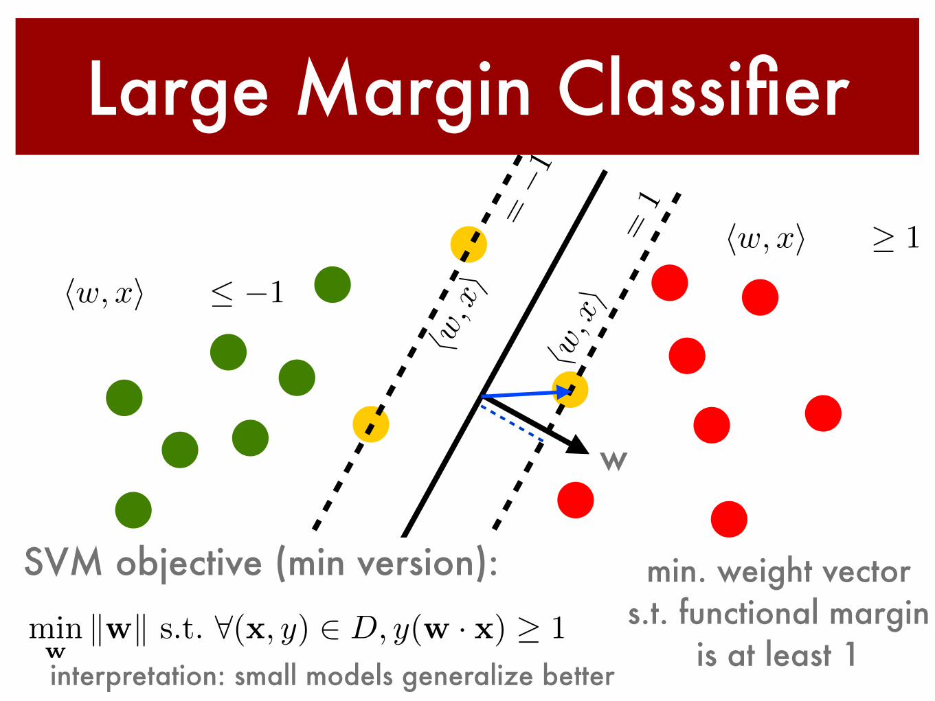
Large Margin Classifier
w
hw, xi+ b � 1
hw, xi+ b �1
SVM objective (min version):
minw
kwk s.t. 8(x, y) 2 D, y(w · x) � 1
interpretation: small models generalize better
min. weight vector s.t. functional margin
is at least 1
hw,
x
i+b
=�1
hw,
x
i+b
=1
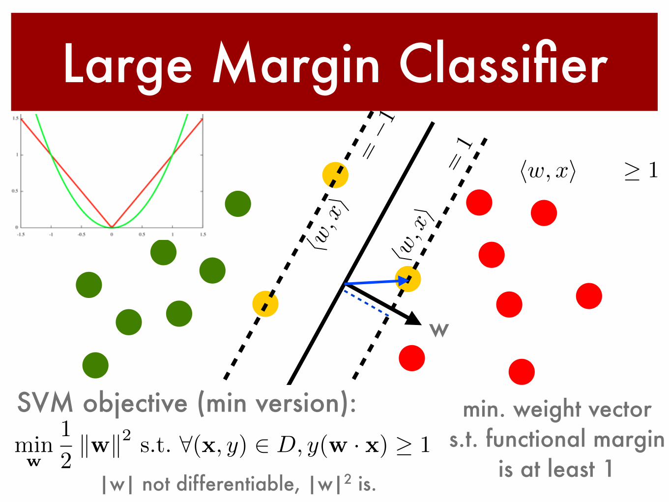
Large Margin Classifier
min. weight vector s.t. functional margin
is at least 1
w
hw, xi+ b � 1hw, xi+ b �1
SVM objective (min version):minw
1
2kwk2 s.t. 8(x, y) 2 D, y(w · x) � 1
|w| not differentiable, |w|2 is.
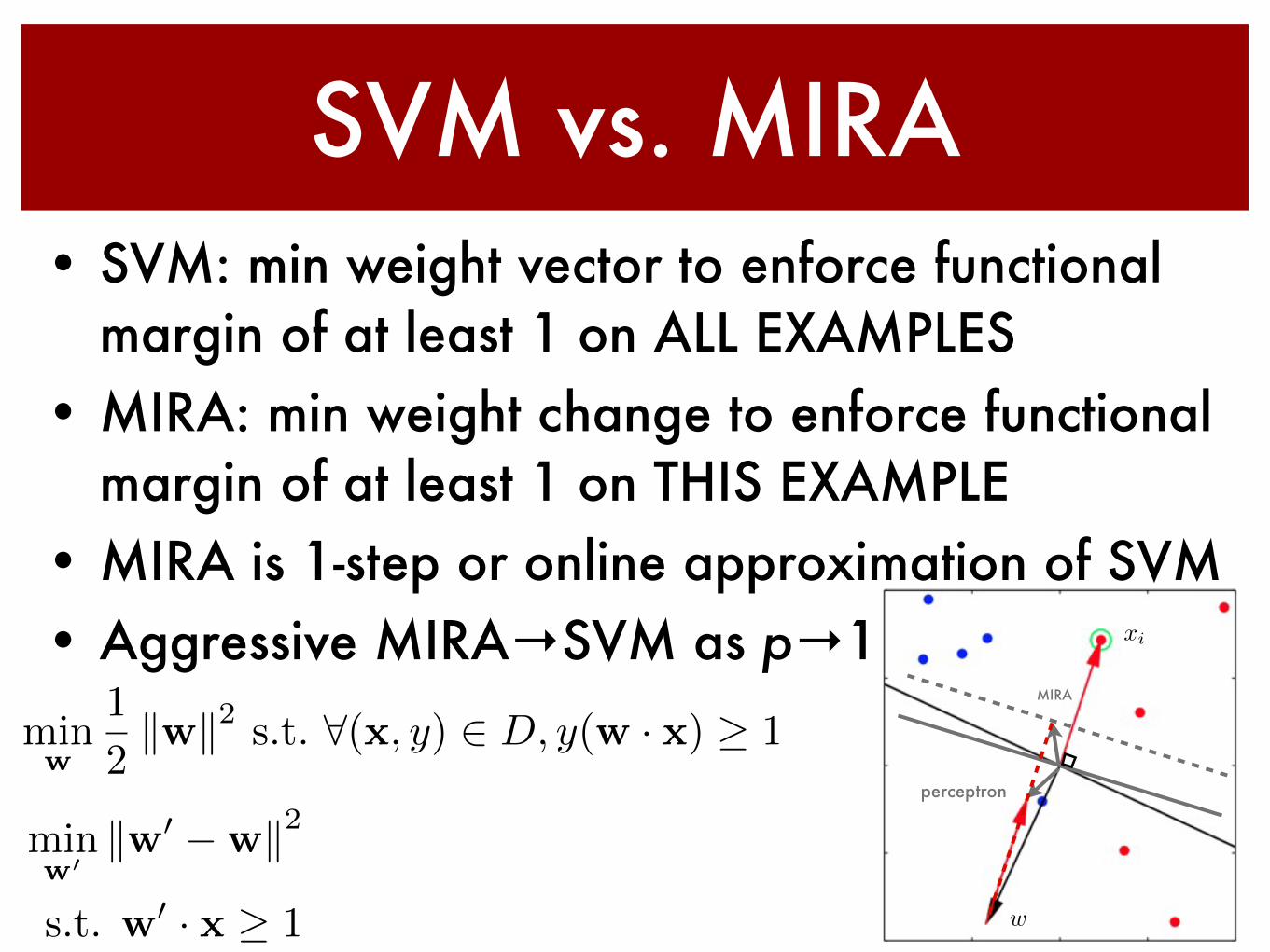
SVM vs. MIRA• SVM: min weight vector to enforce functional
margin of at least 1 on ALL EXAMPLES• MIRA: min weight change to enforce functional
margin of at least 1 on THIS EXAMPLE• MIRA is 1-step or online approximation of SVM• Aggressive MIRA→SVM as p→1minw
1
2kwk2 s.t. 8(x, y) 2 D, y(w · x) � 1
minw0
kw0 �wk2
s.t. w0 · x � 1
xi
w
MIRA
perceptron
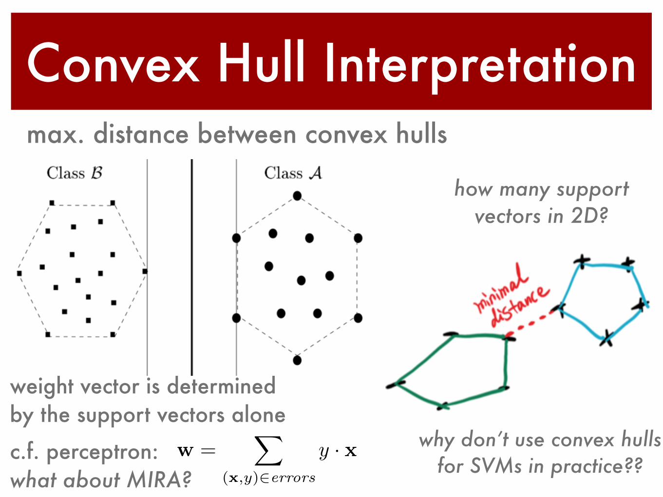
Convex Hull Interpretationmax. distance between convex hulls
why don’t use convex hulls for SVMs in practice??
how many support vectors in 2D?
weight vector is determined by the support vectors alone
c.f. perceptron:what about MIRA?
w =X
(x,y)2errors
y · x
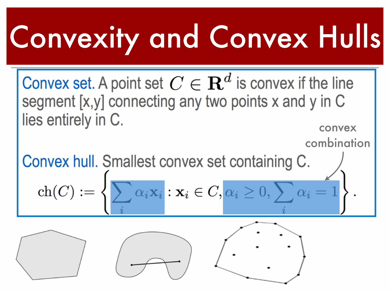
Convexity and Convex Hulls
convex combination
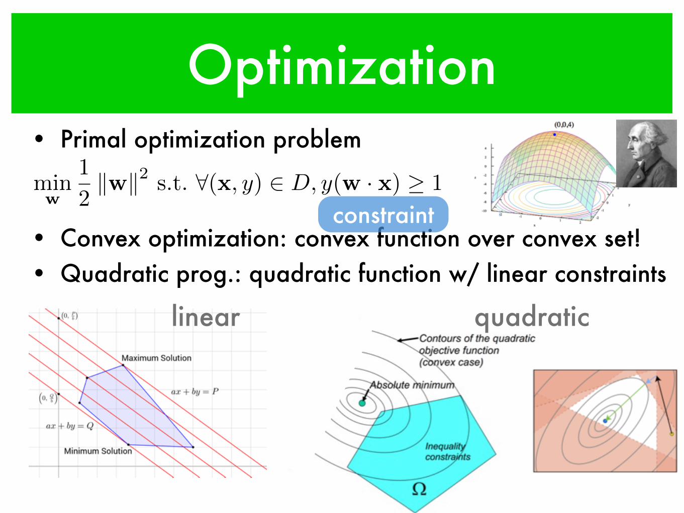
Optimization• Primal optimization problem
• Convex optimization: convex function over convex set!• Quadratic prog.: quadratic function w/ linear constraints
constraintminw
1
2kwk2 s.t. 8(x, y) 2 D, y(w · x) � 1
linear quadratic
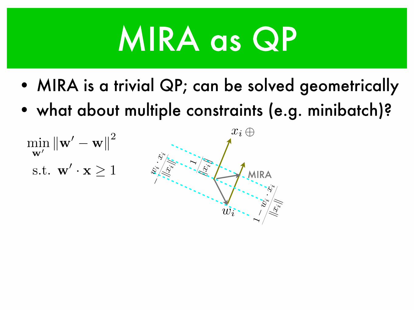
MIRA as QP• MIRA is a trivial QP; can be solved geometrically• what about multiple constraints (e.g. minibatch)?
wi
xi�
MIRA
1kx
ik
�w
i· x
ikx
ik
1�w
i· x
ikx
ik
minw0
kw0 �wk2
s.t. w0 · x � 1
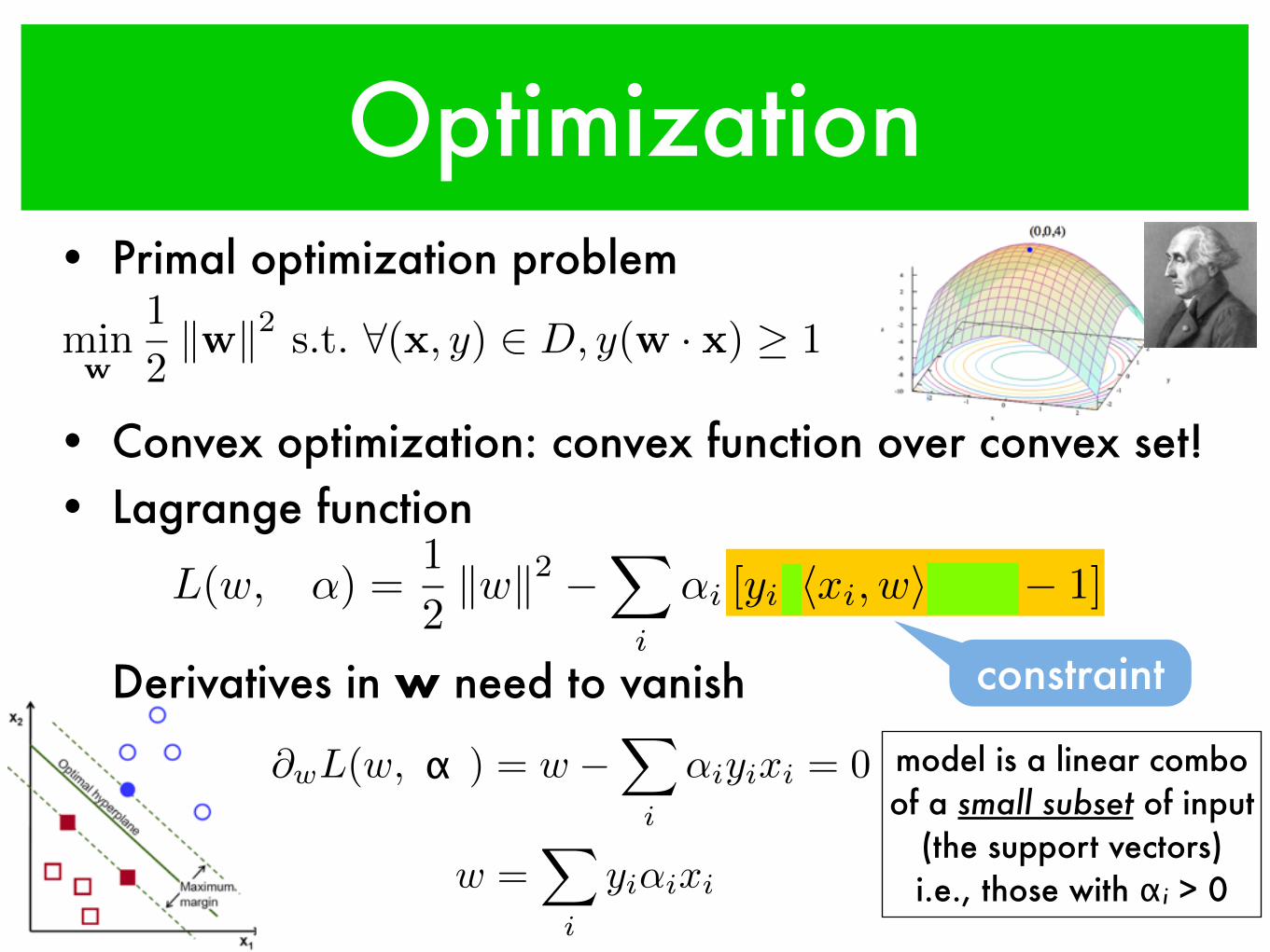
Optimization• Primal optimization problem
• Convex optimization: convex function over convex set!• Lagrange function
Derivatives in w need to vanish constraint
L(w, b,↵) =1
2kwk2 �
X
i
↵i [yi [hxi, wi+ b]� 1]
model is a linear combo of a small subset of input
(the support vectors)i.e., those with αi > 0
minw
1
2kwk2 s.t. 8(x, y) 2 D, y(w · x) � 1
@wL(w, b, a) = w �X
i
↵iyixi = 0
@bL(w, b, a) =X
i
↵iyi = 0w =X
i
yi↵ixi
α
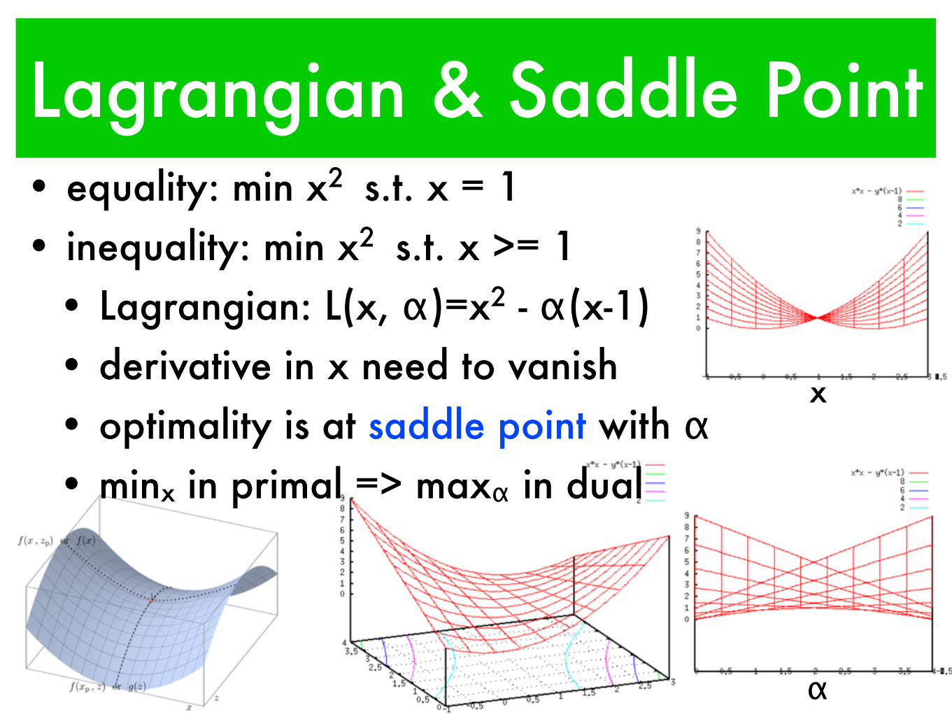
Lagrangian & Saddle Point• equality: min x2 s.t. x = 1• inequality: min x2 s.t. x >= 1
• Lagrangian: L(x, α)=x2 - α(x-1)• derivative in x need to vanish• optimality is at saddle point with α• minx in primal => maxα in dual
α
x

Constrained Optimization
• Quadratic Programming• Quadratic Objective• Linear Constraints
KKT condition (complementary slackness)optimal point is achieved at active constraints
where αi > 0 (αi=0 => inactive)
↵i [yi [hw, xii+ b]� 1] = 0
minimize
w,b
1
2
kwk2 subject to yi [hxi, wi+ b] � 1
w =X
i
yi↵ixi
constraint
Karush–Kuhn–Tucker
w
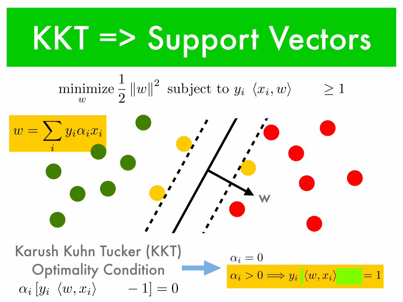
KKT => Support Vectorsminimize
w,b
1
2
kwk2 subject to yi [hxi, wi+ b] � 1
w =X
i
yi↵ixi
Karush Kuhn Tucker (KKT) Optimality Condition
↵i = 0
↵i > 0 =) yi [hw, xii+ b] = 1↵i [yi [hw, xii+ b]� 1] = 0
w
w =X
i
yi↵ixi
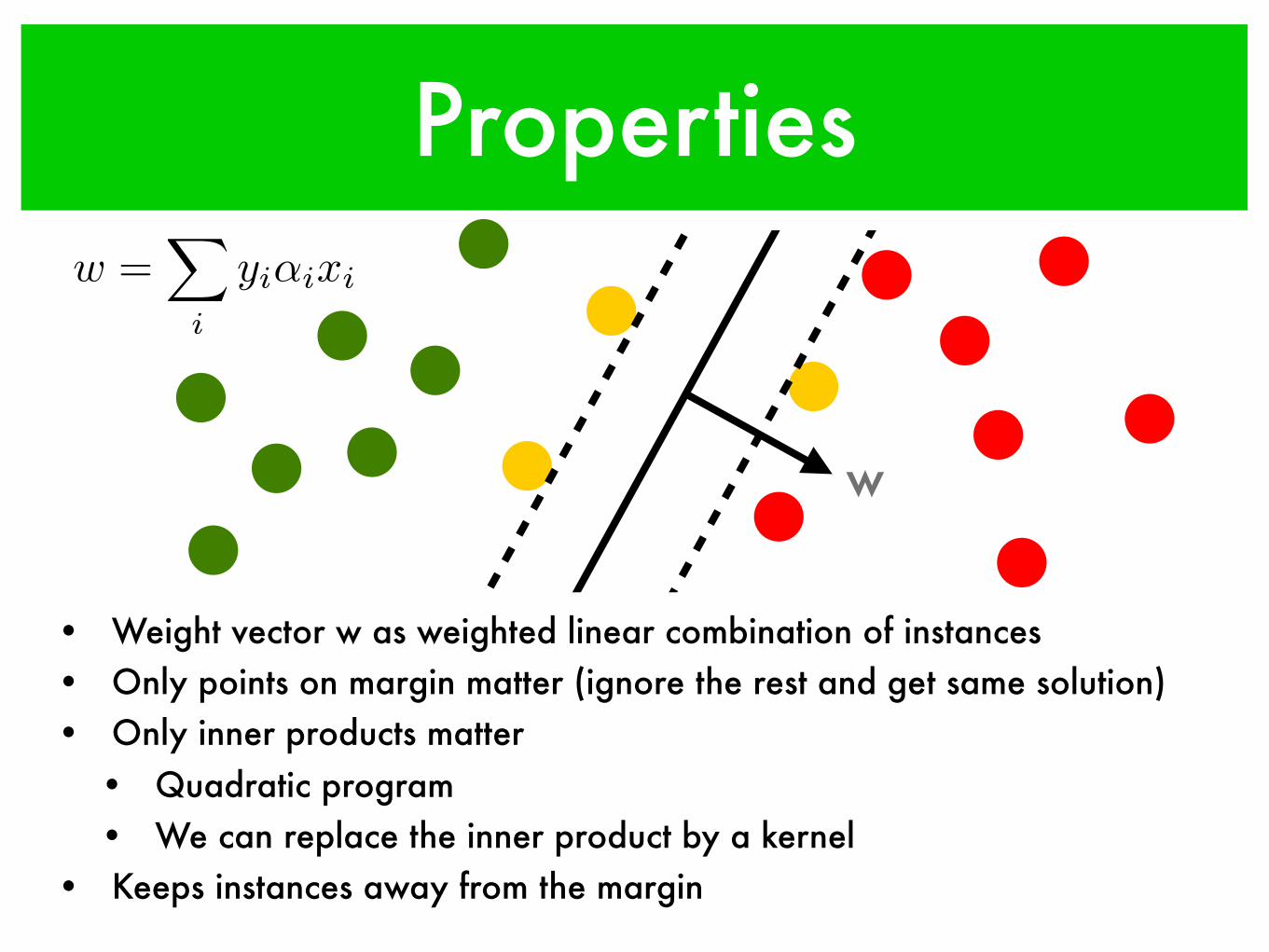
Properties
• Weight vector w as weighted linear combination of instances• Only points on margin matter (ignore the rest and get same solution)• Only inner products matter
• Quadratic program• We can replace the inner product by a kernel
• Keeps instances away from the margin
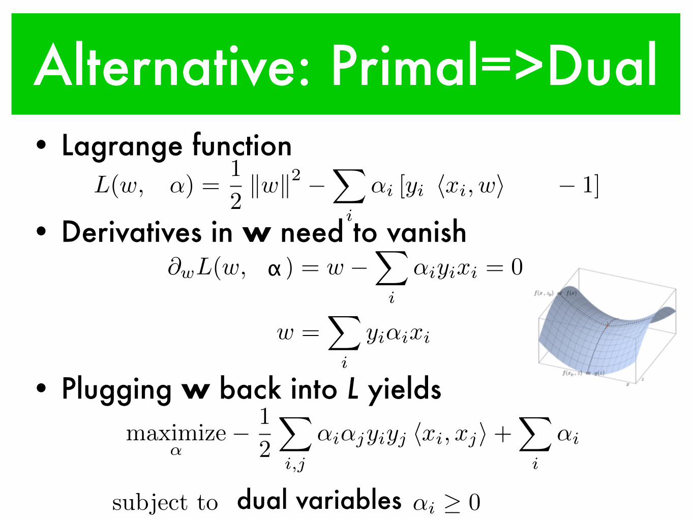
Alternative: Primal=>Dual• Lagrange function
• Derivatives in w need to vanish
• Plugging w back into L yields
L(w, b,↵) =1
2kwk2 �
X
i
↵i [yi [hxi, wi+ b]� 1]
maximize
↵� 1
2
X
i,j
↵i↵jyiyj hxi, xji+X
i
↵i
subject to
X
i
↵iyi = 0 and ↵i � 0
@wL(w, b, a) = w �X
i
↵iyixi = 0
@bL(w, b, a) =X
i
↵iyi = 0w =X
i
yi↵ixi
dual variables
α
w
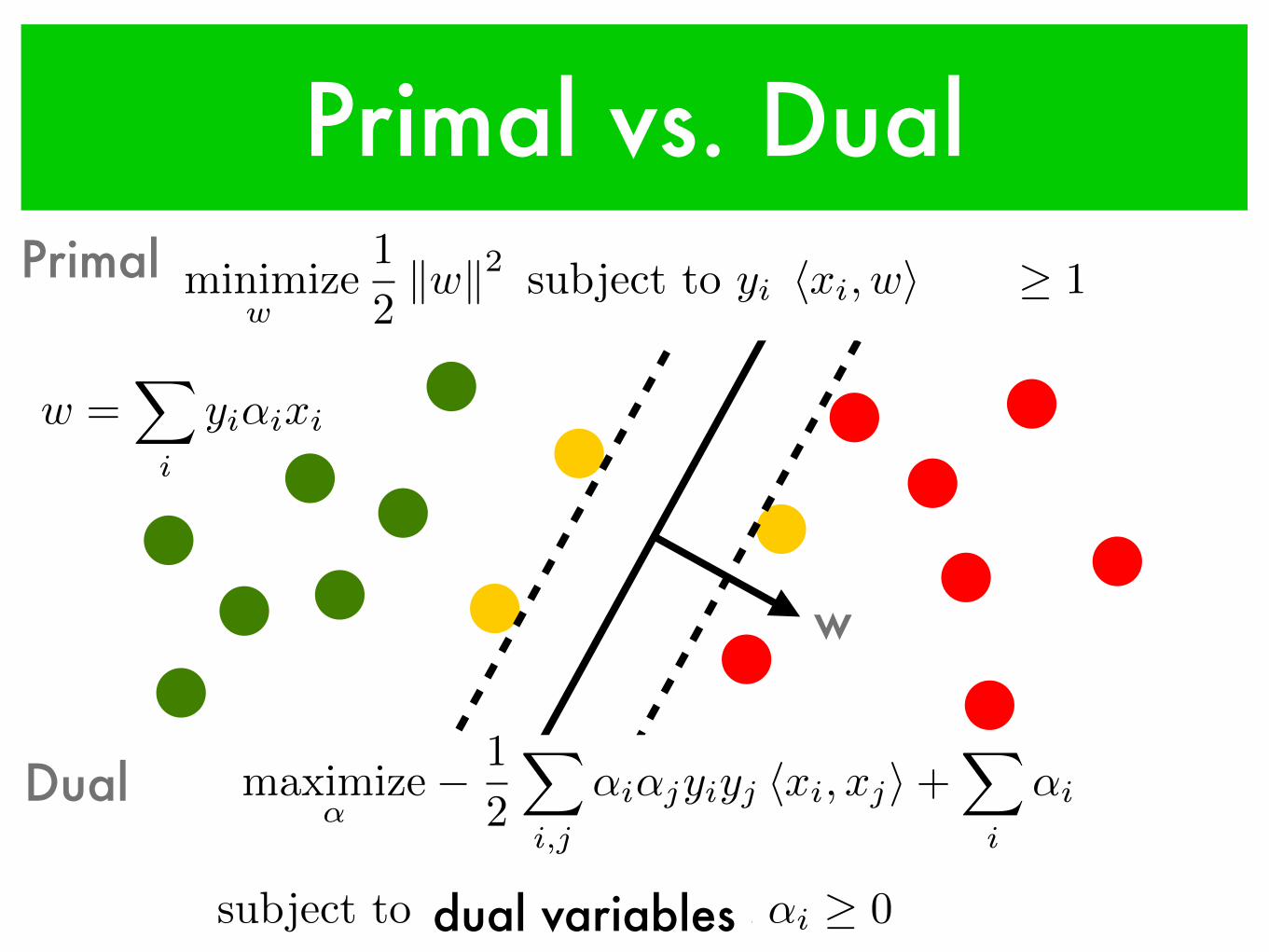
Primal vs. Dual
w =X
i
yi↵ixi
maximize
↵� 1
2
X
i,j
↵i↵jyiyj hxi, xji+X
i
↵i
subject to
X
i
↵iyi = 0 and ↵i � 0dual variables
minimize
w,b
1
2
kwk2 subject to yi [hxi, wi+ b] � 1
Primal
Dual
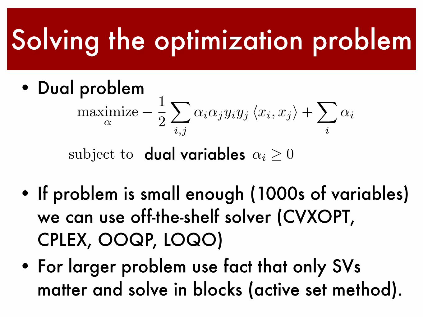
Solving the optimization problem• Dual problem
• If problem is small enough (1000s of variables) we can use off-the-shelf solver (CVXOPT, CPLEX, OOQP, LOQO)
• For larger problem use fact that only SVs matter and solve in blocks (active set method).
maximize
↵� 1
2
X
i,j
↵i↵jyiyj hxi, xji+X
i
↵i
subject to
X
i
↵iyi = 0 and ↵i � 0dual variables
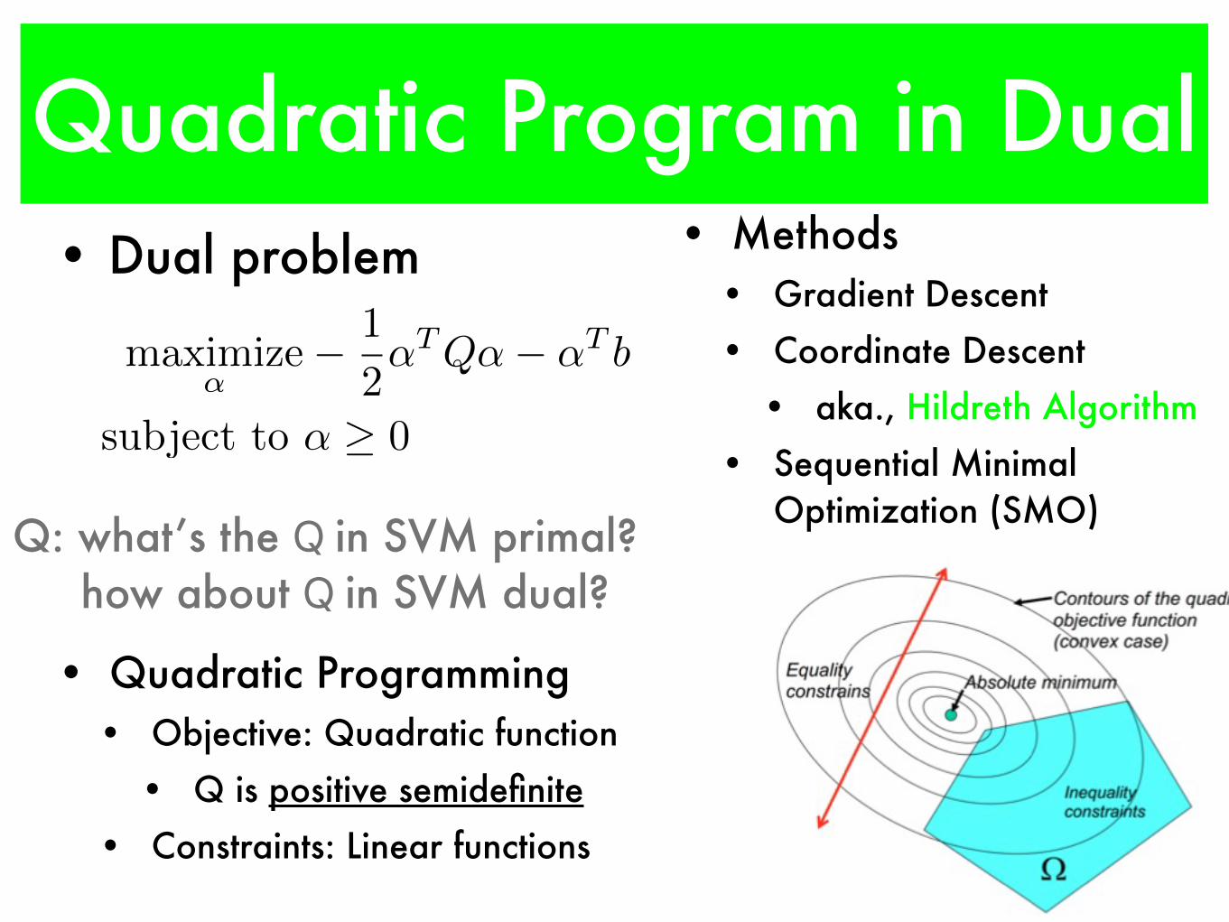
Quadratic Program in Dual• Dual problem
maximize
↵� 1
2
↵TQ↵� ↵T b
subject to ↵ � 0
• Quadratic Programming• Objective: Quadratic function
• Q is positive semidefinite• Constraints: Linear functions
• Methods• Gradient Descent• Coordinate Descent
• aka., Hildreth Algorithm• Sequential Minimal
Optimization (SMO)Q: what’s the Q in SVM primal? how about Q in SVM dual?
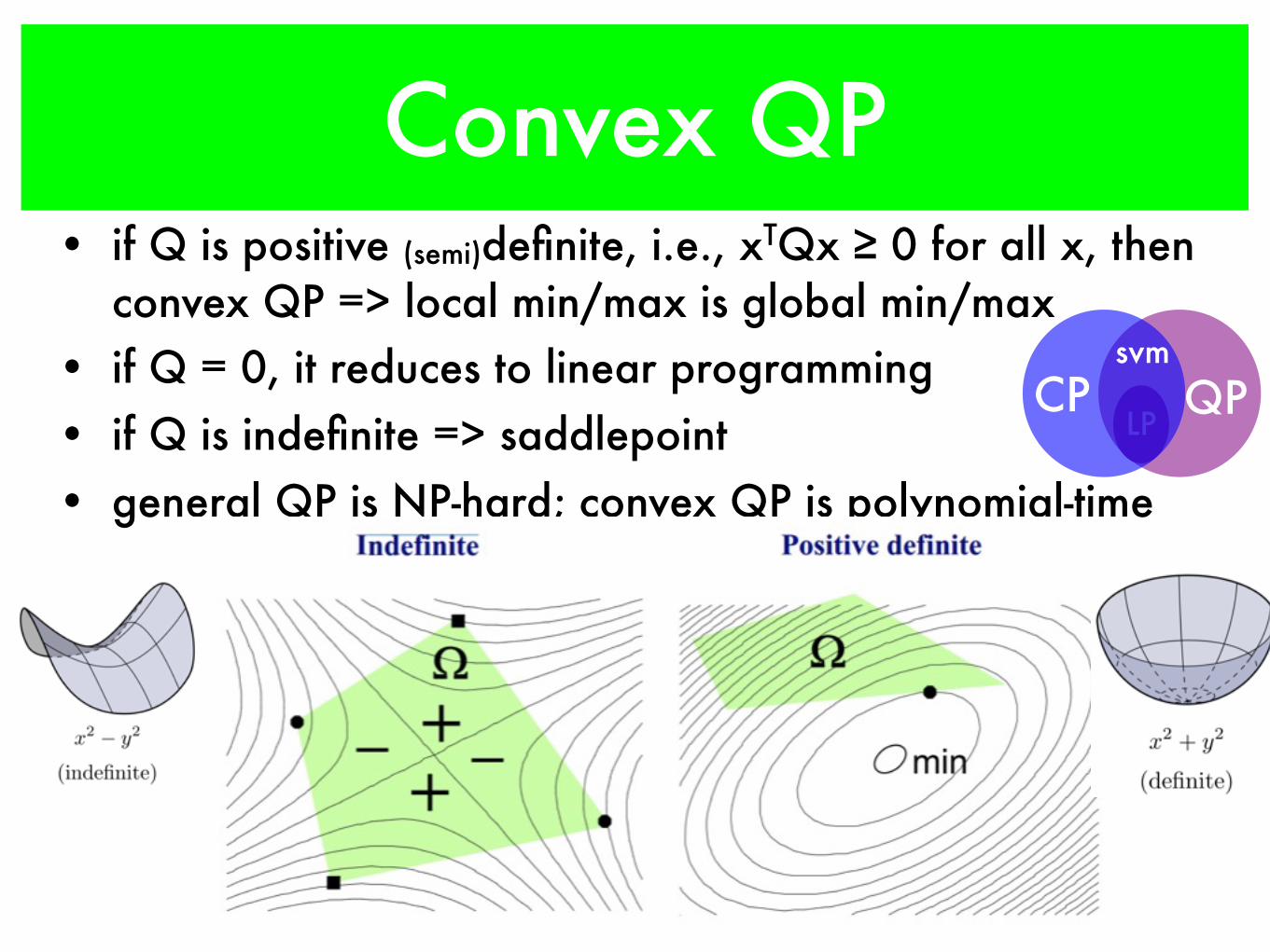
Convex QP• if Q is positive (semi)definite, i.e., xTQx ≥ 0 for all x, then
convex QP => local min/max is global min/max• if Q = 0, it reduces to linear programming• if Q is indefinite => saddlepoint• general QP is NP-hard; convex QP is polynomial-time
LP QPCP
svm
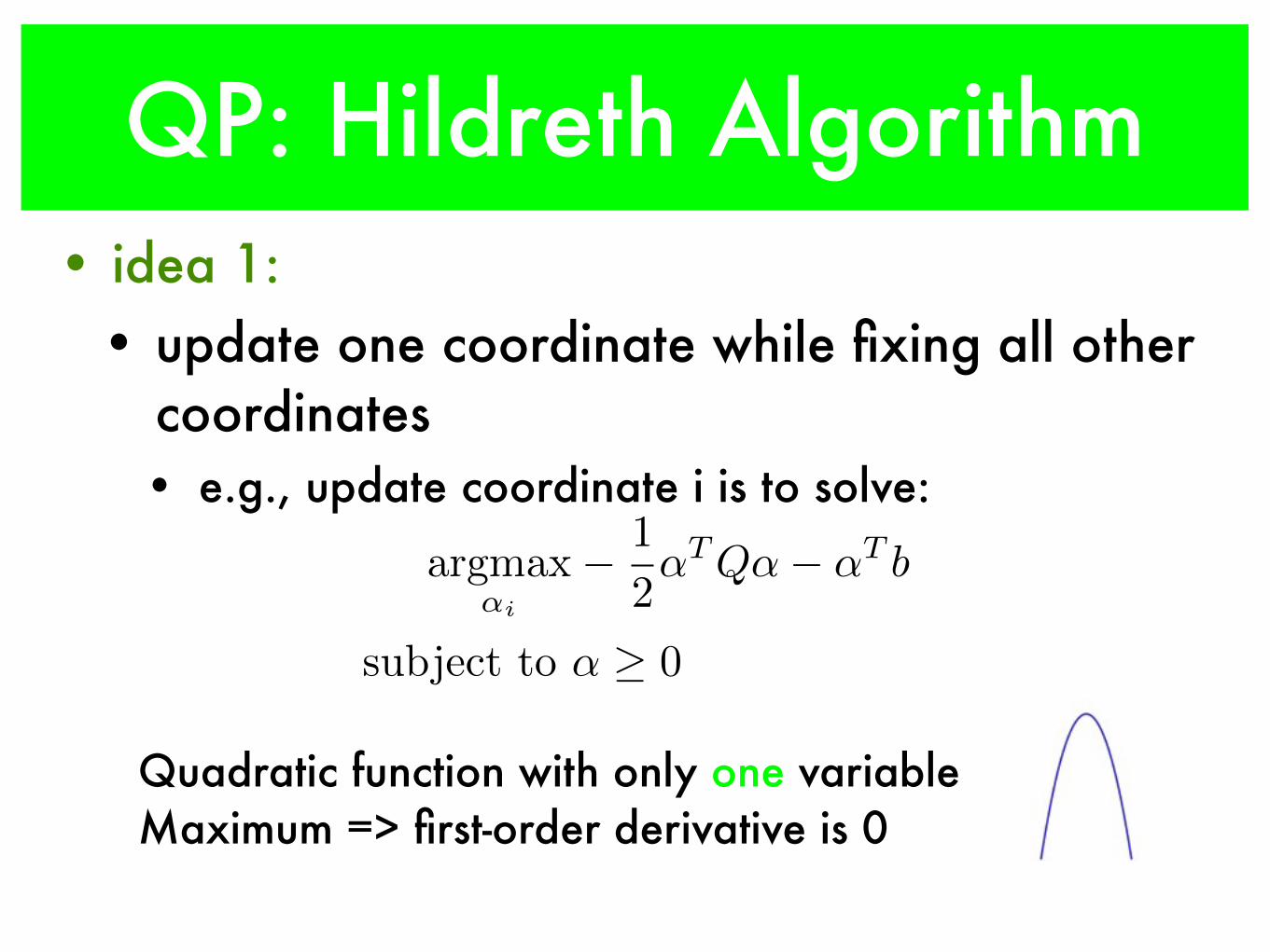
QP: Hildreth Algorithm• idea 1:
• update one coordinate while fixing all other coordinates• e.g., update coordinate i is to solve:
argmax
↵i
� 1
2
↵TQ↵� ↵T b
subject to ↵ � 0
Quadratic function with only one variableMaximum => first-order derivative is 0
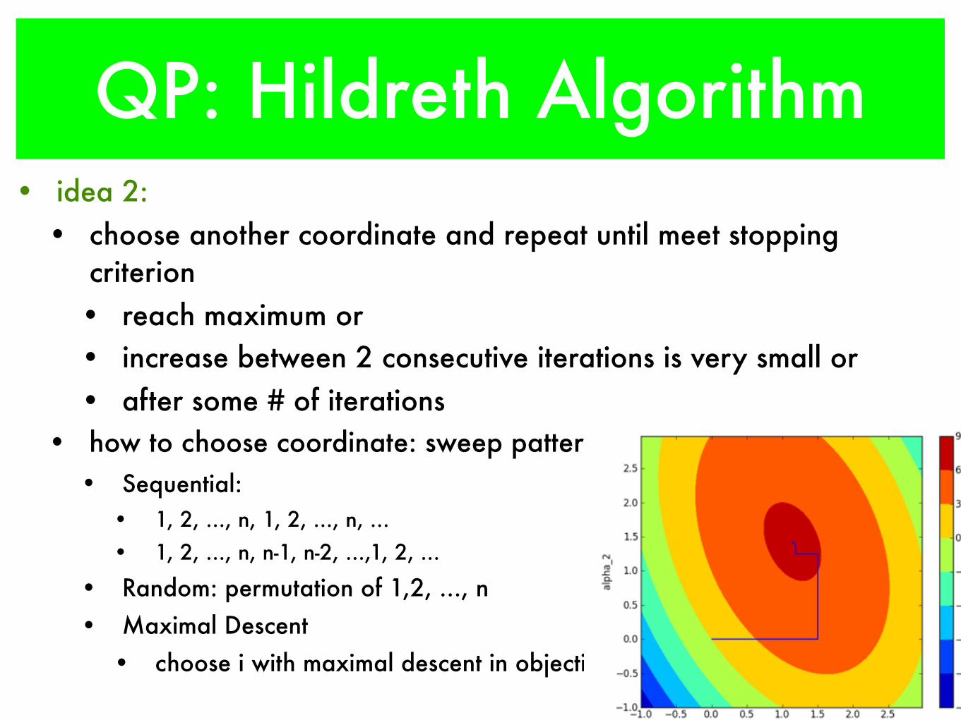
QP: Hildreth Algorithm• idea 2:
• choose another coordinate and repeat until meet stopping criterion
• reach maximum or • increase between 2 consecutive iterations is very small or • after some # of iterations
• how to choose coordinate: sweep pattern• Sequential:
• 1, 2, ..., n, 1, 2, ..., n, ...• 1, 2, ..., n, n-1, n-2, ...,1, 2, ...
• Random: permutation of 1,2, ..., n• Maximal Descent
• choose i with maximal descent in objective
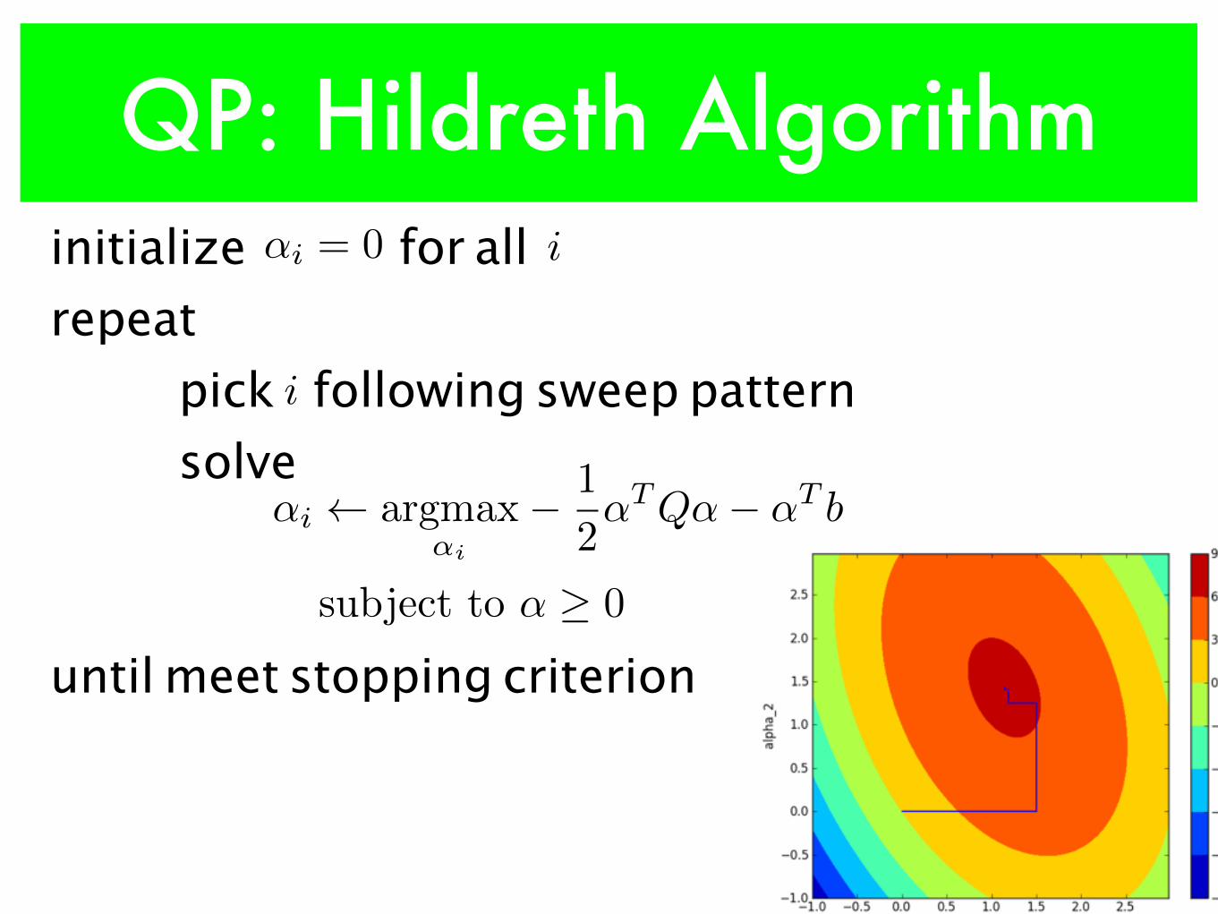
QP: Hildreth Algorithm
i
initialize for all repeat
pick following sweep patternsolve
until meet stopping criterion
↵i argmax
↵i
� 1
2
↵TQ↵� ↵T b
subject to ↵ � 0
↵i = 0 i
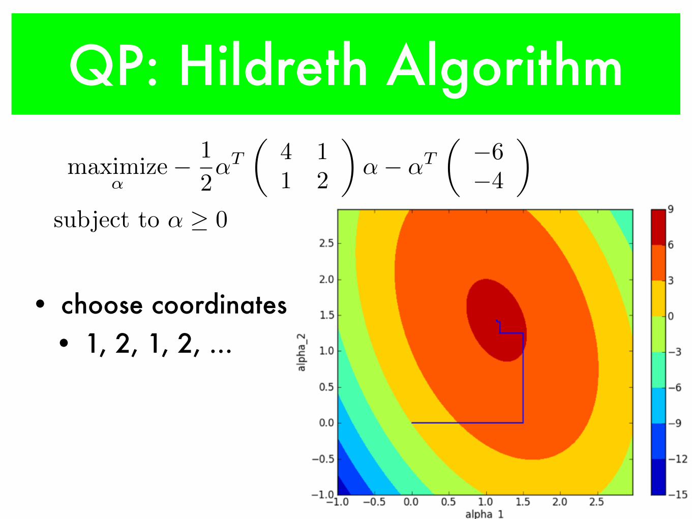
QP: Hildreth Algorithm
• choose coordinates • 1, 2, 1, 2, ...
maximize
↵� 1
2
↵T
✓4 1
1 2
◆↵� ↵T
✓�6
�4
◆
subject to ↵ � 0
QP: Hildreth Algorithm• pros:
• extremely simple• no gradient calculation• easy to implement
• cons:• converges slow, compared to other methods• can’t deal with too many constraints
• works for minibatch MIRA but not SVM
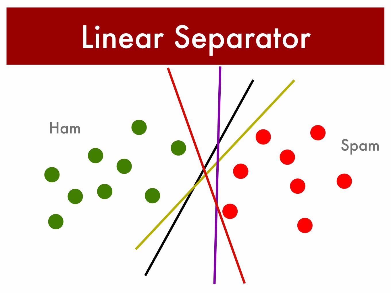
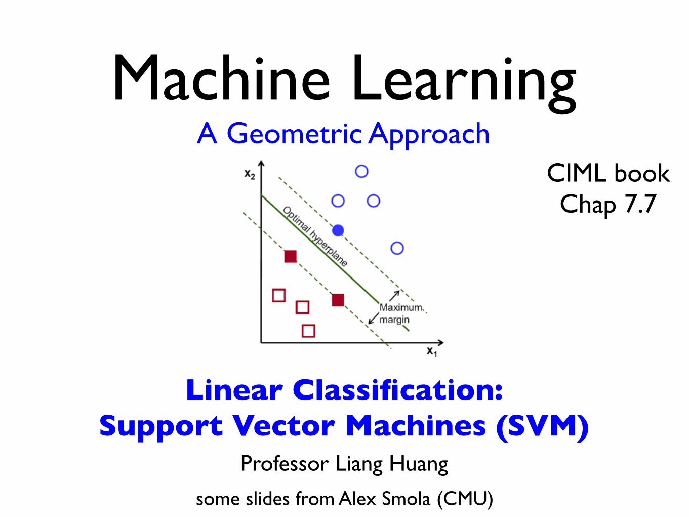
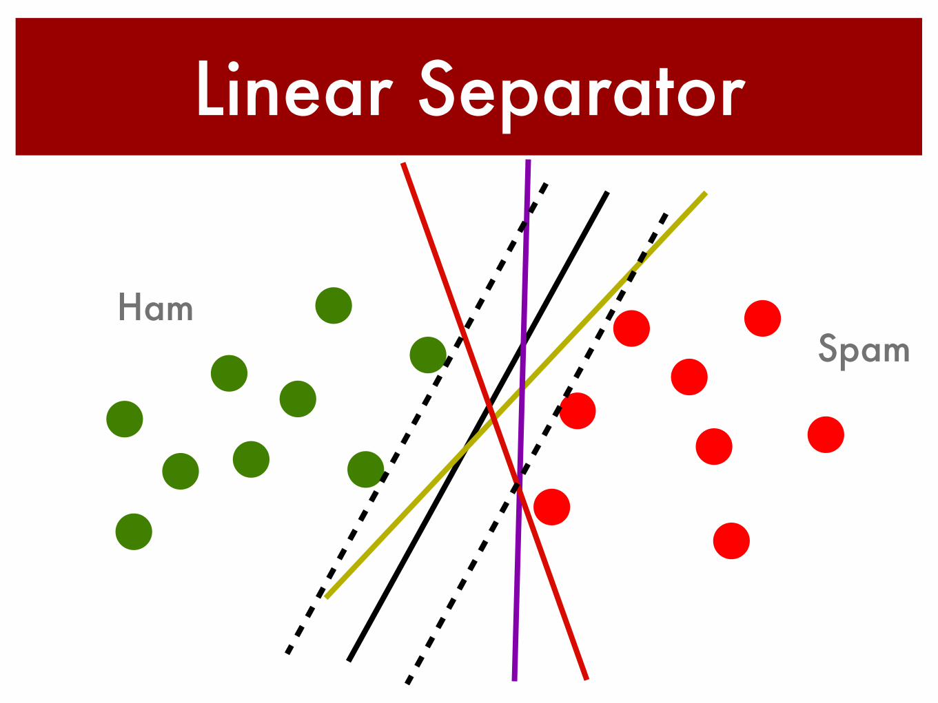
Linear Separator
SpamHam

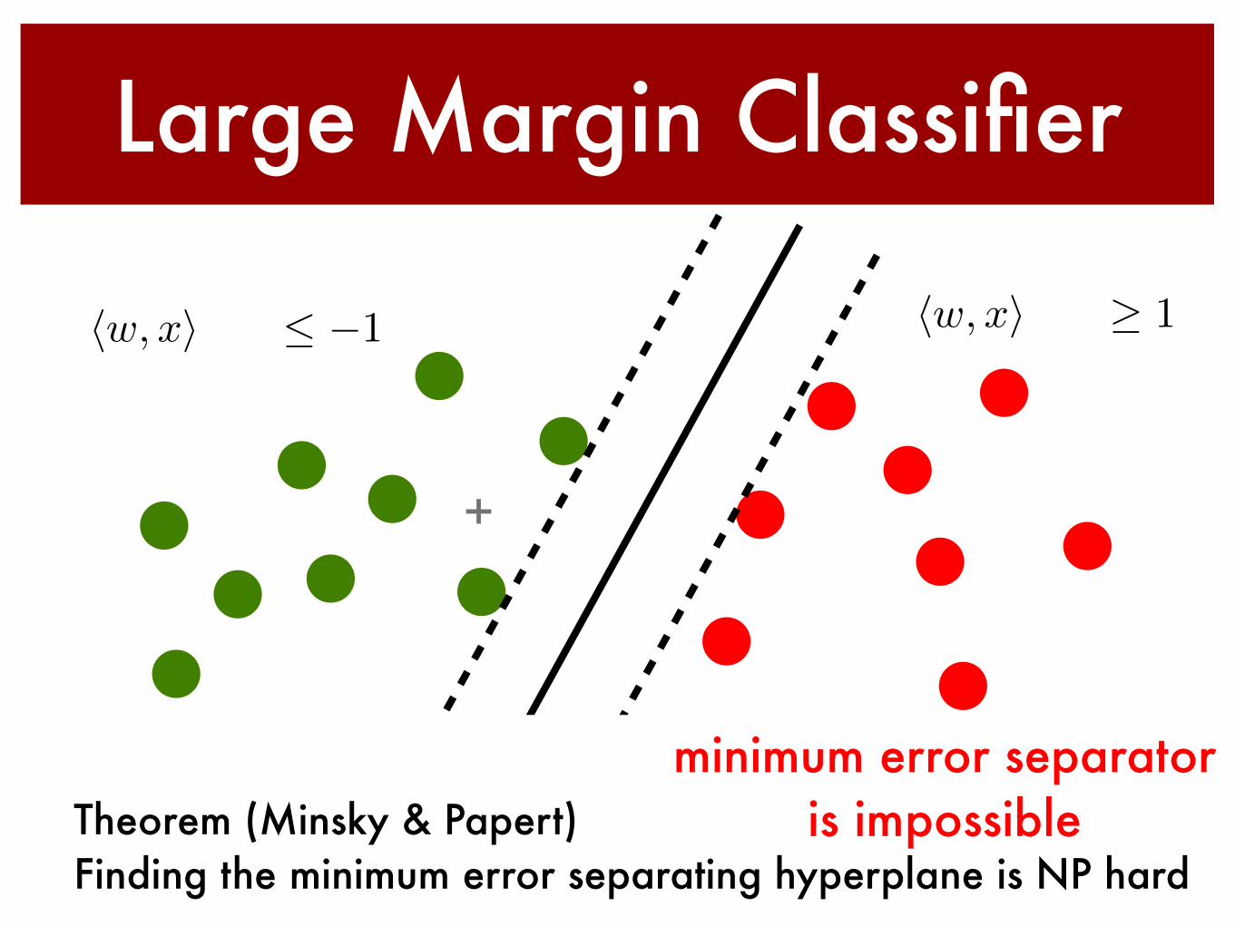
Large Margin Classifier
hw, xi+ b �1 hw, xi+ b � 1
f(x) = hw, xi+ b
linear functionlinear separator
is impossible
++
Large Margin Classifier
hw, xi+ b �1 hw, xi+ b � 1
Theorem (Minsky & Papert)Finding the minimum error separating hyperplane is NP hard
minimum error separatoris impossible
+
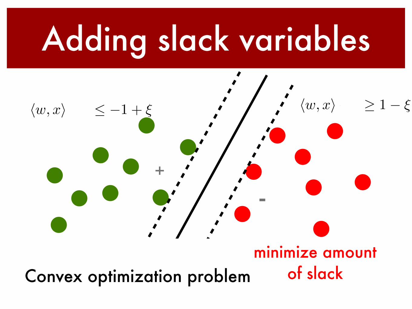
hw, xi+ b �1 + ⇠
Adding slack variables
Convex optimization problemminimize amount
of slack
hw, xi+ b � 1� ⇠
+
-
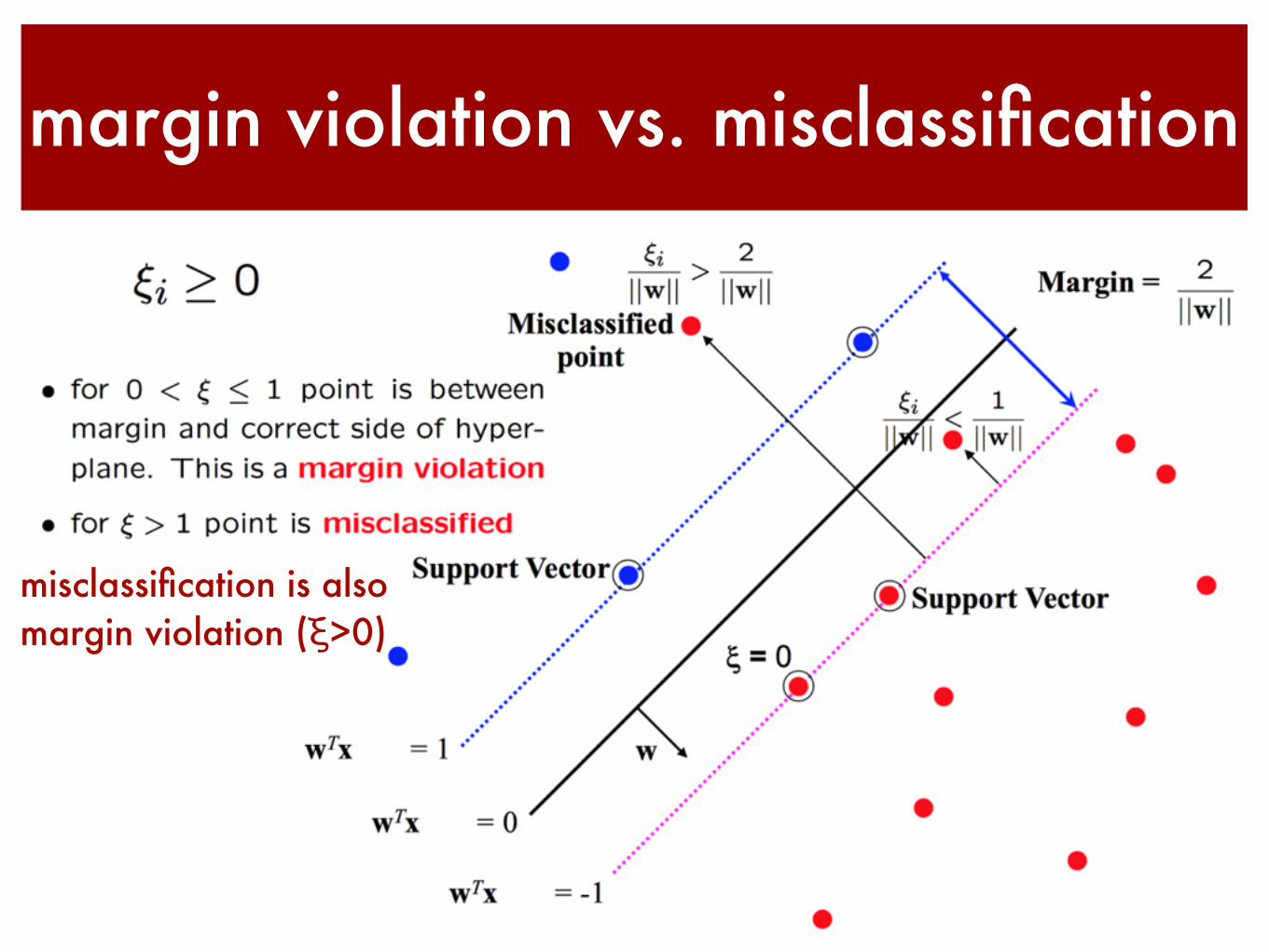
margin violation vs. misclassification
misclassification is also margin violation (ξ>0)
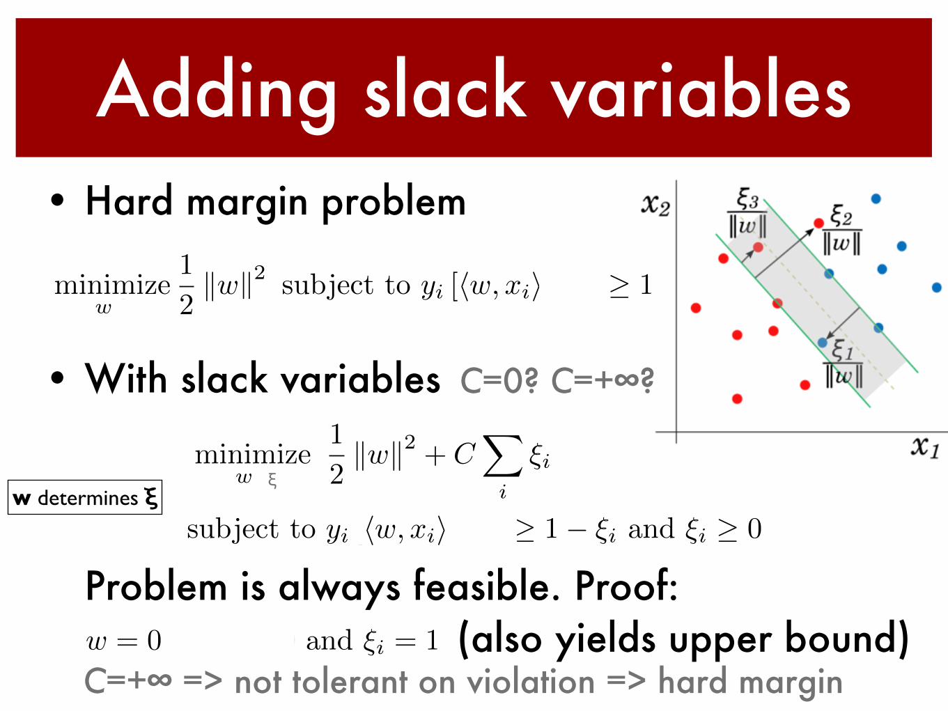
Adding slack variables• Hard margin problem
• With slack variables
Problem is always feasible. Proof: (also yields upper bound)
minimize
w,b
1
2
kwk2 + C
X
i
⇠i
subject to yi [hw, xii+ b] � 1� ⇠i and ⇠i � 0
w = 0 and b = 0 and ⇠i = 1
minimize
w,b
1
2
kwk2 subject to yi [hw, xii+ b] � 1
C=0? C=+∞?
C=+∞ => not tolerant on violation => hard margin
ξw determines ξ
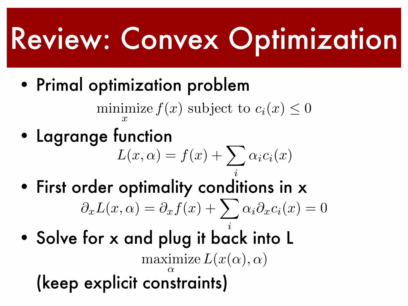
Review: Convex Optimization• Primal optimization problem
• Lagrange function
• First order optimality conditions in x
• Solve for x and plug it back into L
(keep explicit constraints)
minimize
x
f(x) subject to c
i
(x) 0
L(x,↵) = f(x) +X
i
↵ici(x)
@
x
L(x,↵) = @
x
f(x) +X
i
↵
i
@
x
c
i
(x) = 0
maximize
↵L(x(↵),↵)
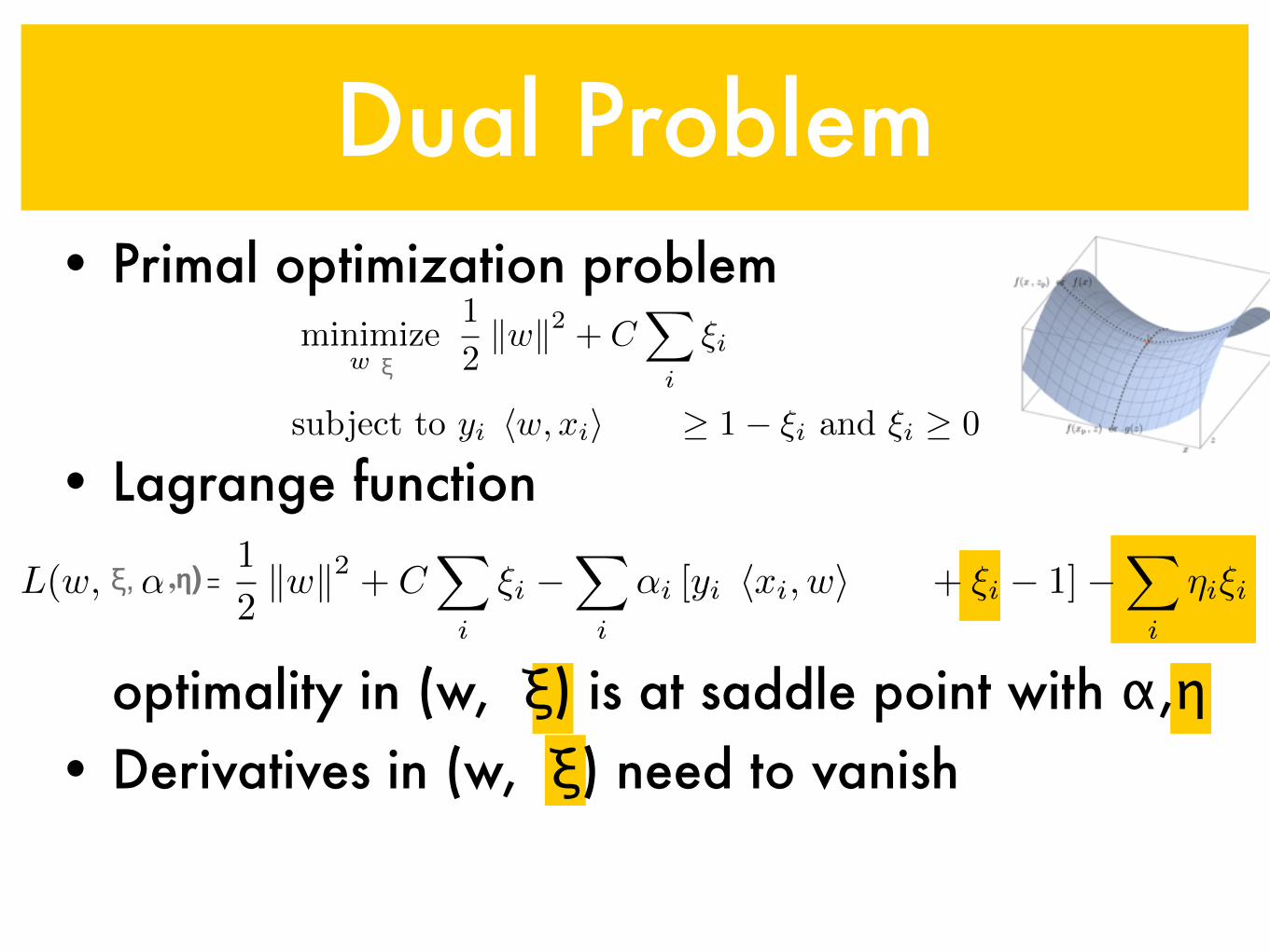
• Primal optimization problem
• Lagrange function
optimality in (w, ξ) is at saddle point with α,η• Derivatives in (w, ξ) need to vanish
L(w, b,↵) =1
2kwk2 + C
X
i
⇠i �X
i
↵i [yi [hxi, wi+ b] + ⇠i � 1]�X
i
⌘i⇠i
Dual Problem
minimize
w,b
1
2
kwk2 + C
X
i
⇠i
subject to yi [hw, xii+ b] � 1� ⇠i and ⇠i � 0
ξ
ξ, ,𝝶)
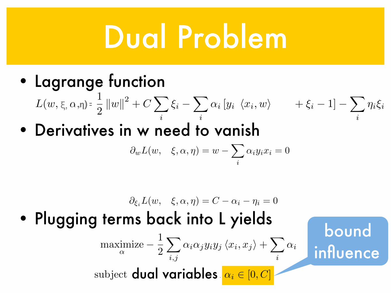
Dual Problem• Lagrange function
• Derivatives in w need to vanish
• Plugging terms back into L yields
@wL(w, b, ⇠,↵, ⌘) = w �X
i
↵iyixi = 0
@bL(w, b, ⇠,↵, ⌘) =X
i
↵iyi = 0
@⇠iL(w, b, ⇠,↵, ⌘) = C � ↵i � ⌘i = 0
maximize
↵� 1
2
X
i,j
↵i↵jyiyj hxi, xji+X
i
↵i
subject to
X
i
↵iyi = 0 and ↵i 2 [0, C]
boundinfluence
dual variables
L(w, b,↵) =1
2kwk2 + C
X
i
⇠i �X
i
↵i [yi [hxi, wi+ b] + ⇠i � 1]�X
i
⌘i⇠iξ, ,𝝶)
w
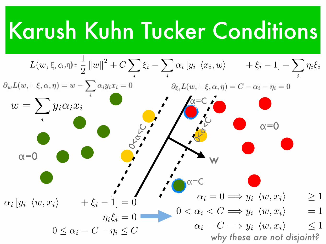
Karush Kuhn Tucker Conditions
w =X
i
yi↵ixi
↵i [yi [hw, xii+ b] + ⇠i � 1] = 0
⌘i⇠i = 0
0 ↵i = C � ⌘i C
L(w, b,↵) =1
2kwk2 + C
X
i
⇠i �X
i
↵i [yi [hxi, wi+ b] + ⇠i � 1]�X
i
⌘i⇠i
↵i = 0 =) yi [hw, xii+ b] � 1
0 < ↵i < C =) yi [hw, xii+ b] = 1
↵i = C =) yi [hw, xii+ b] 1
ξ,
why these are not disjoint?
α=0
α=00<α<
C
0<α<
C
α=C
α=C
,𝝶)
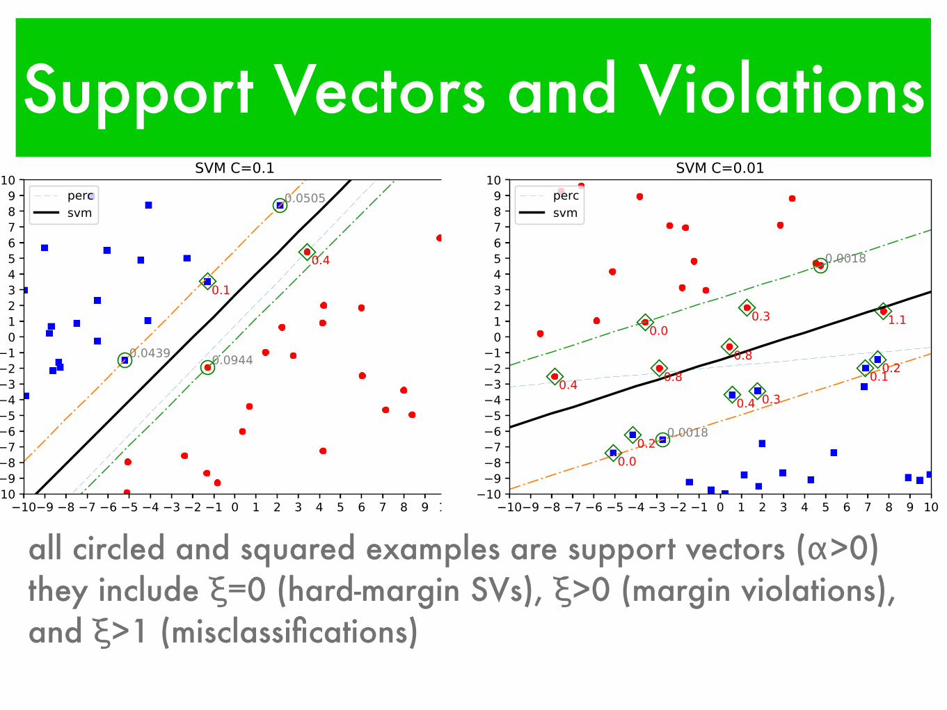
Support Vectors and Violations
all circled and squared examples are support vectors (α>0)they include ξ=0 (hard-margin SVs), ξ>0 (margin violations), and ξ>1 (misclassifications)
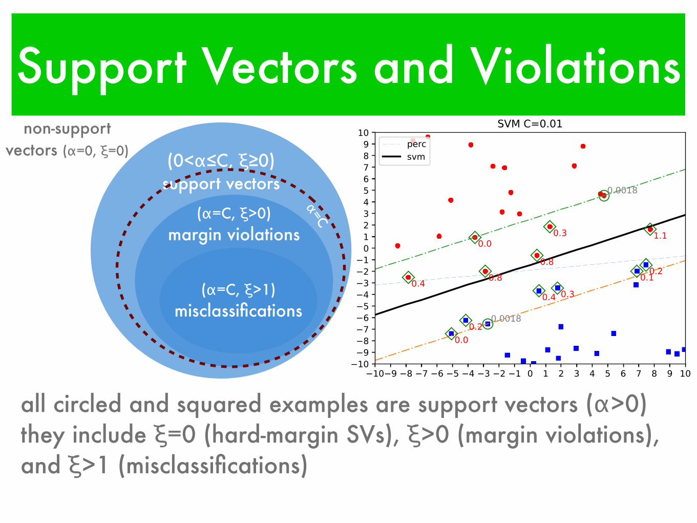
Support Vectors and Violations
all circled and squared examples are support vectors (α>0)they include ξ=0 (hard-margin SVs), ξ>0 (margin violations), and ξ>1 (misclassifications)
(0<α≤C, ξ≥0) support vectors
(α=C, ξ>0)
margin violations
non-support vectors (α=0, ξ=0)
(α=C, ξ>1) misclassifications
α=C
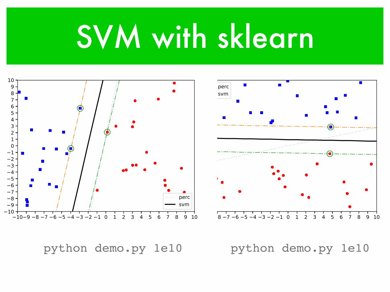
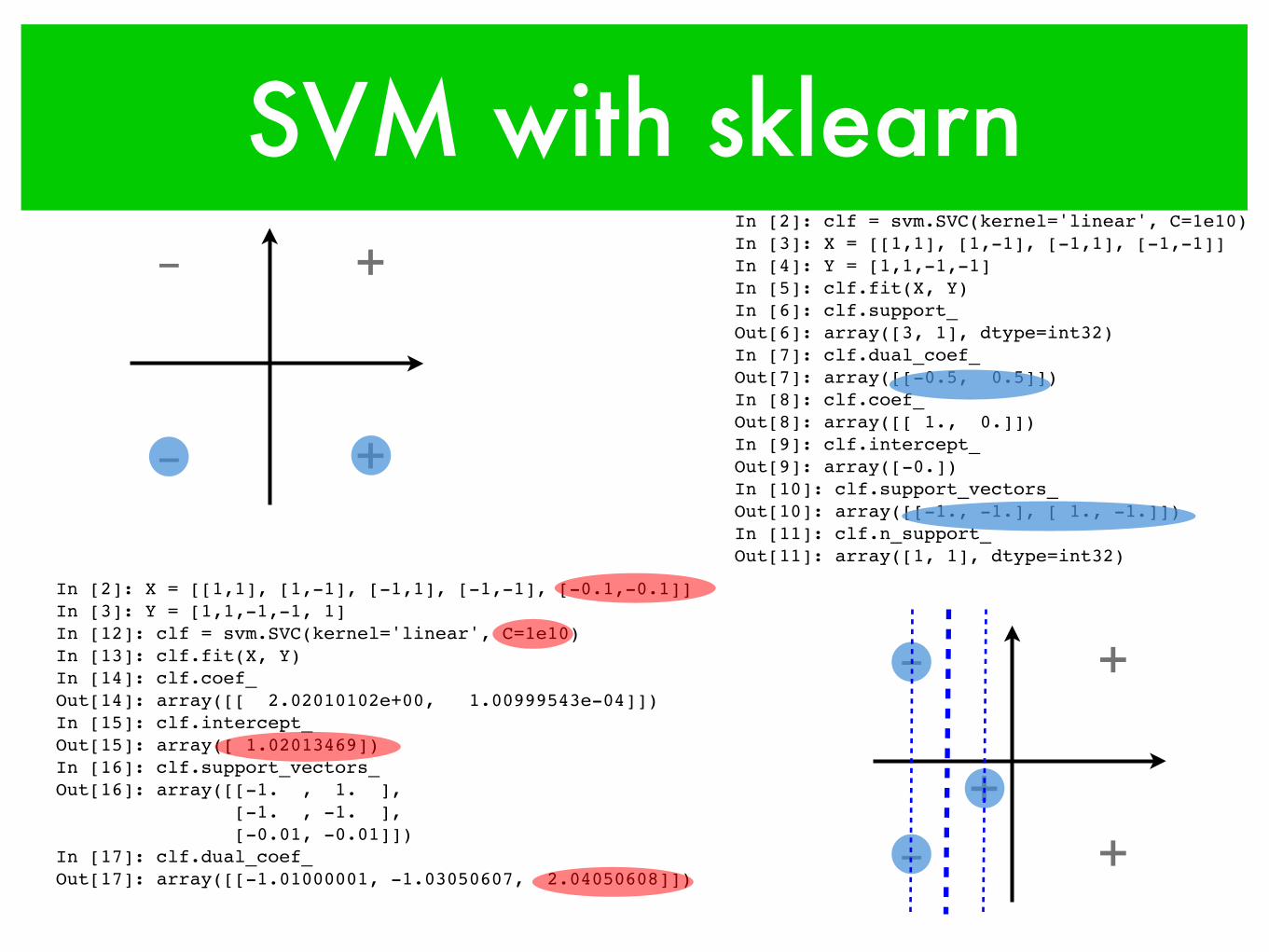
SVM with sklearn
python demo.py 1e10 python demo.py 1e10

SVM with sklearnpython demo.py 0.01python demo.py 0.1
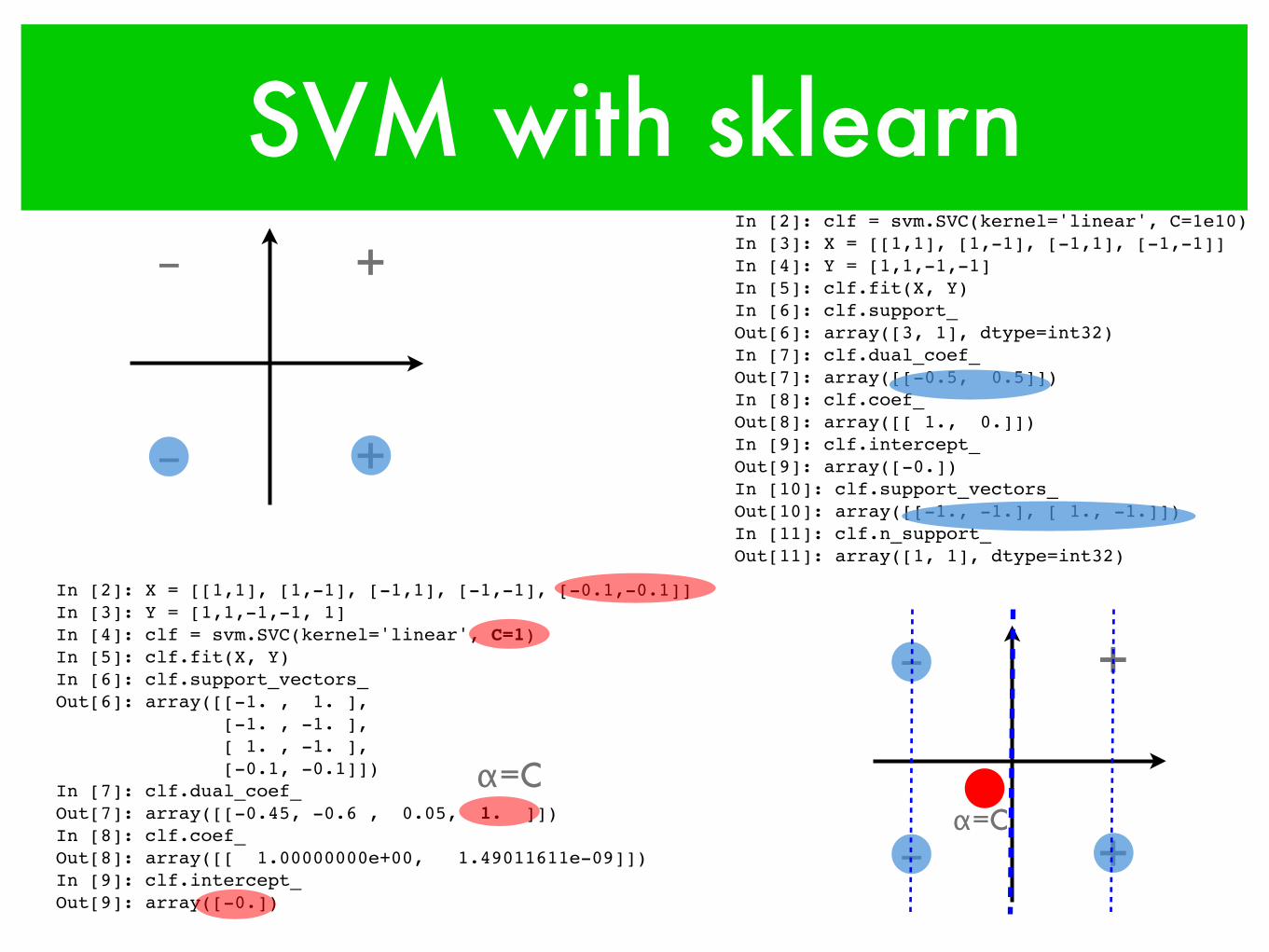
SVM with sklearn
+
+‒
‒
+
+‒
‒In [2]: clf = svm.SVC(kernel='linear', C=1e10)In [3]: X = [[1,1], [1,-1], [-1,1], [-1,-1]]In [4]: Y = [1,1,-1,-1]In [5]: clf.fit(X, Y)In [6]: clf.support_Out[6]: array([3, 1], dtype=int32)In [7]: clf.dual_coef_Out[7]: array([[-0.5, 0.5]])In [8]: clf.coef_Out[8]: array([[ 1., 0.]])In [9]: clf.intercept_Out[9]: array([-0.])In [10]: clf.support_vectors_Out[10]: array([[-1., -1.], [ 1., -1.]])In [11]: clf.n_support_Out[11]: array([1, 1], dtype=int32)
+
In [2]: X = [[1,1], [1,-1], [-1,1], [-1,-1], [-0.1,-0.1]]In [3]: Y = [1,1,-1,-1, 1]In [4]: clf = svm.SVC(kernel='linear', C=1)In [5]: clf.fit(X, Y)In [6]: clf.support_vectors_Out[6]: array([[-1. , 1. ], [-1. , -1. ], [ 1. , -1. ], [-0.1, -0.1]])In [7]: clf.dual_coef_Out[7]: array([[-0.45, -0.6 , 0.05, 1. ]])In [8]: clf.coef_Out[8]: array([[ 1.00000000e+00, 1.49011611e-09]])In [9]: clf.intercept_Out[9]: array([-0.])
α=Cα=C
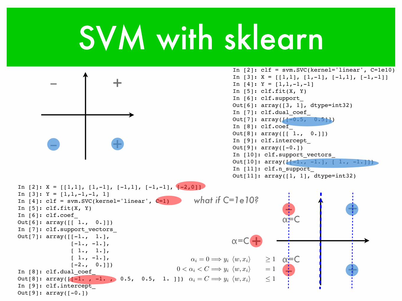
SVM with sklearn
+
+‒
‒
+
+‒
‒In [2]: clf = svm.SVC(kernel='linear', C=1e10)In [3]: X = [[1,1], [1,-1], [-1,1], [-1,-1]]In [4]: Y = [1,1,-1,-1]In [5]: clf.fit(X, Y)In [6]: clf.support_Out[6]: array([3, 1], dtype=int32)In [7]: clf.dual_coef_Out[7]: array([[-0.5, 0.5]])In [8]: clf.coef_Out[8]: array([[ 1., 0.]])In [9]: clf.intercept_Out[9]: array([-0.])In [10]: clf.support_vectors_Out[10]: array([[-1., -1.], [ 1., -1.]])In [11]: clf.n_support_Out[11]: array([1, 1], dtype=int32)
+
In [2]: X = [[1,1], [1,-1], [-1,1], [-1,-1], [-0.1,-0.1]]In [3]: Y = [1,1,-1,-1, 1]In [12]: clf = svm.SVC(kernel='linear', C=1e10)In [13]: clf.fit(X, Y)In [14]: clf.coef_Out[14]: array([[ 2.02010102e+00, 1.00999543e-04]])In [15]: clf.intercept_Out[15]: array([ 1.02013469])In [16]: clf.support_vectors_Out[16]: array([[-1. , 1. ], [-1. , -1. ], [-0.01, -0.01]])In [17]: clf.dual_coef_Out[17]: array([[-1.01000001, -1.03050607, 2.04050608]])
SVM with sklearn
+
+‒
‒
+
+‒
‒In [2]: clf = svm.SVC(kernel='linear', C=1e10)In [3]: X = [[1,1], [1,-1], [-1,1], [-1,-1]]In [4]: Y = [1,1,-1,-1]In [5]: clf.fit(X, Y)In [6]: clf.support_Out[6]: array([3, 1], dtype=int32)In [7]: clf.dual_coef_Out[7]: array([[-0.5, 0.5]])In [8]: clf.coef_Out[8]: array([[ 1., 0.]])In [9]: clf.intercept_Out[9]: array([-0.])In [10]: clf.support_vectors_Out[10]: array([[-1., -1.], [ 1., -1.]])In [11]: clf.n_support_Out[11]: array([1, 1], dtype=int32)
+
In [2]: X = [[1,1], [1,-1], [-1,1], [-1,-1], [-2,0]]In [3]: Y = [1,1,-1,-1, 1]In [4]: clf = svm.SVC(kernel='linear', C=1)In [5]: clf.fit(X, Y)In [6]: clf.coef_Out[6]: array([[ 1., 0.]])In [7]: clf.support_vectors_Out[7]: array([[-1., 1.], [-1., -1.], [ 1., 1.], [ 1., -1.], [-2., 0.]])In [8]: clf.dual_coef_Out[8]: array([[-1. , -1. , 0.5, 0.5, 1. ]])In [9]: clf.intercept_Out[9]: array([-0.])
α=C
α=C
α=C
↵i = 0 =) yi [hw, xii+ b] � 1
0 < ↵i < C =) yi [hw, xii+ b] = 1
↵i = C =) yi [hw, xii+ b] 1
what if C=1e10?
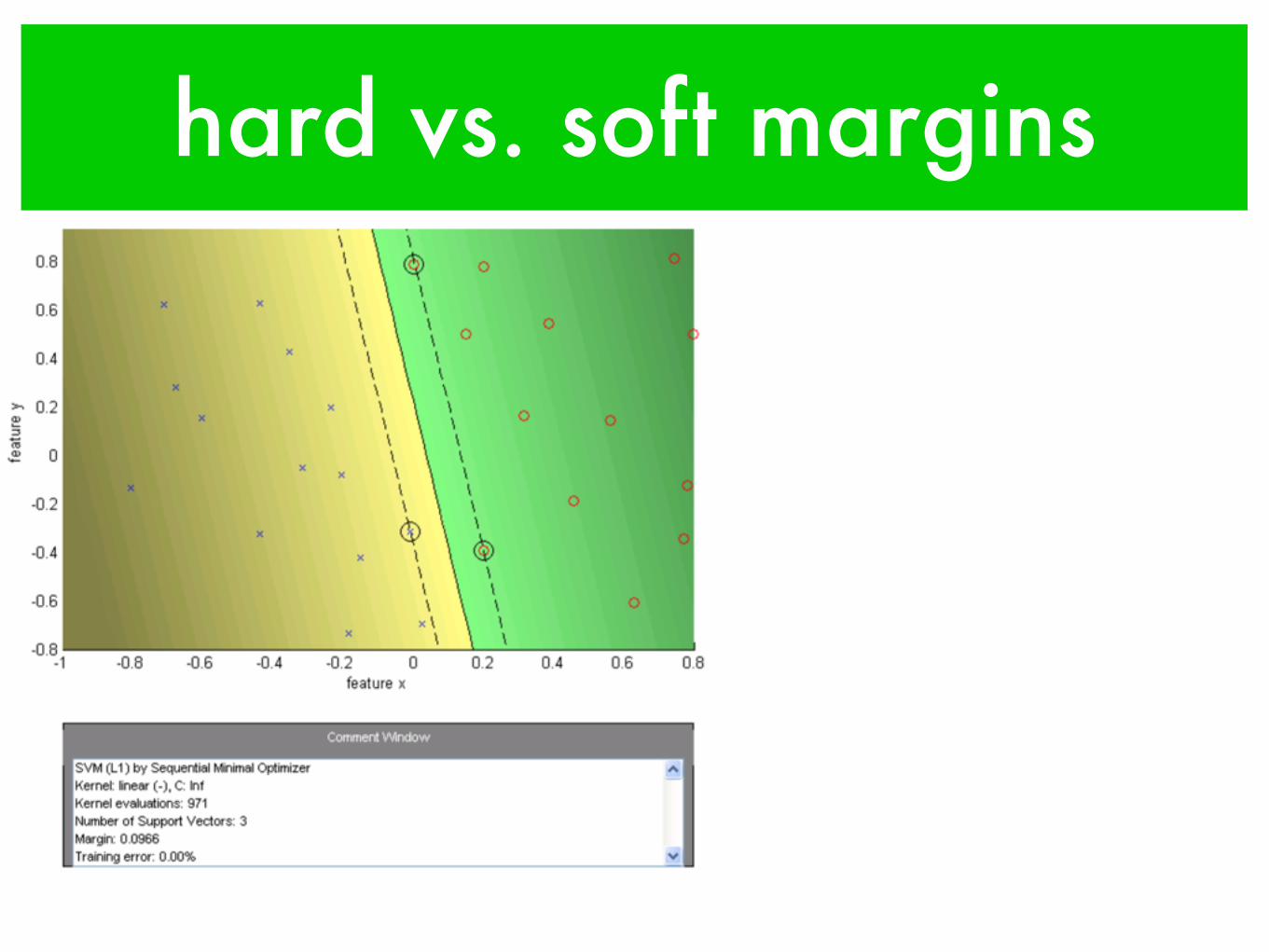
hard vs. soft margins
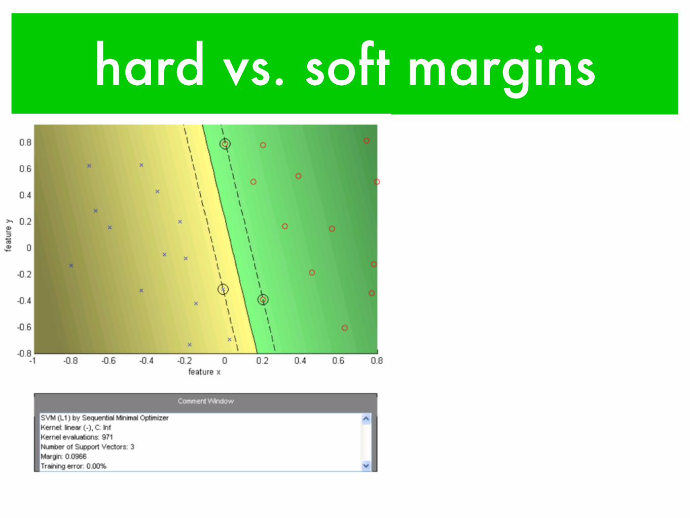
hard vs. soft margins
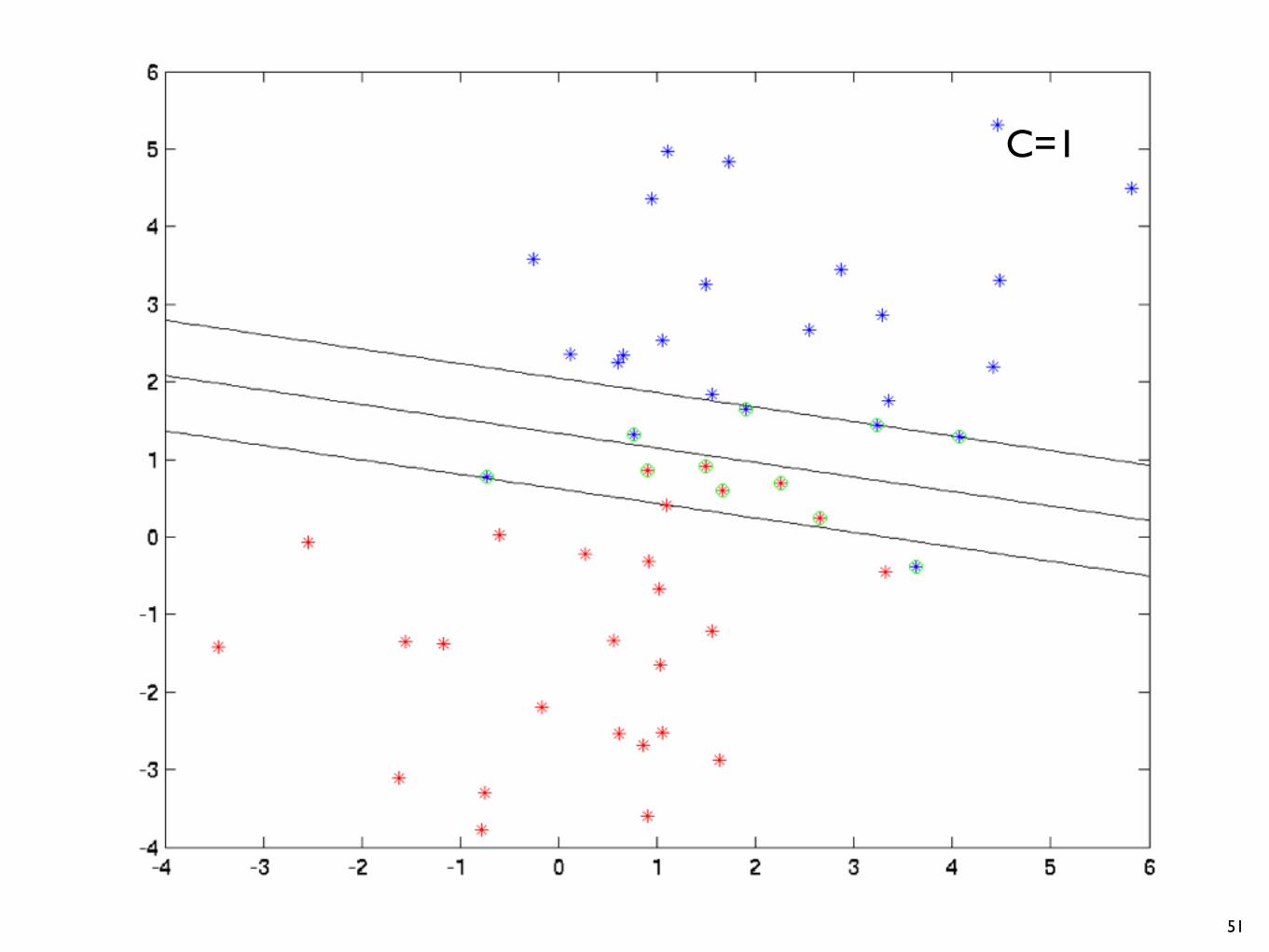
C=1
51

C=20
52
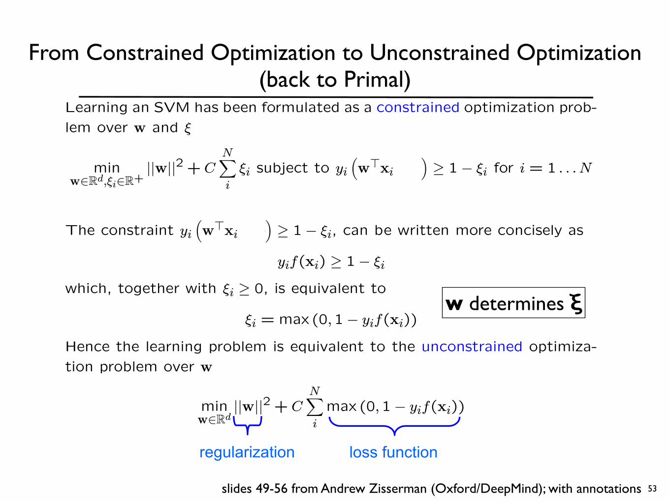
OptimizationLearning an SVM has been formulated as a constrained optimization prob-
lem over w and ξ
minw∈Rd,ξi∈R+
||w||2 + CNX
i
ξi subject to yi³w>xi+ b
´≥ 1− ξi for i = 1 . . . N
The constraint yi³w>xi+ b
´≥ 1− ξi, can be written more concisely as
yif(xi) ≥ 1− ξi
which, together with ξi ≥ 0, is equivalent to
ξi = max (0,1− yif(xi))
Hence the learning problem is equivalent to the unconstrained optimiza-
tion problem over w
minw∈Rd
||w||2 + CNX
i
max (0,1− yif(xi))
loss functionregularization
From Constrained Optimization to Unconstrained Optimization(back to Primal)
53slides 49-56 from Andrew Zisserman (Oxford/DeepMind); with annotations
w determines ξ
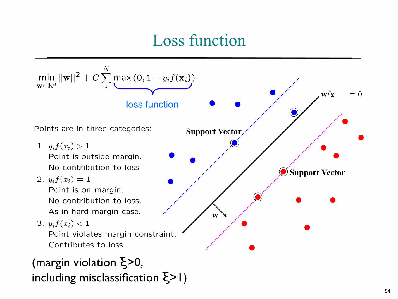
Loss function
w
Support Vector
Support Vector
wTx + b = 0
minw∈Rd
||w||2 + CNX
i
max (0,1− yif(xi))
Points are in three categories:
1. yif(xi) > 1
Point is outside margin.
No contribution to loss
2. yif(xi) = 1
Point is on margin.
No contribution to loss.
As in hard margin case.
3. yif(xi) < 1
Point violates margin constraint.
Contributes to loss
loss function
54
(margin violation ξ>0, including misclassification ξ>1)
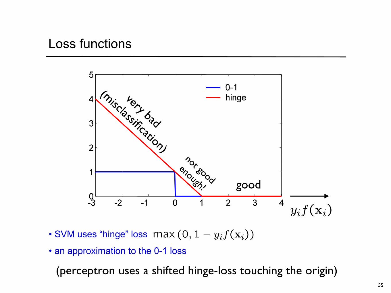
Loss functions
• SVM uses “hinge” loss
• an approximation to the 0-1 loss
max (0,1− yif(xi))
yif(xi)
55
good
very bad
(misclassification)not good
enough!
(perceptron uses a shifted hinge-loss touching the origin)
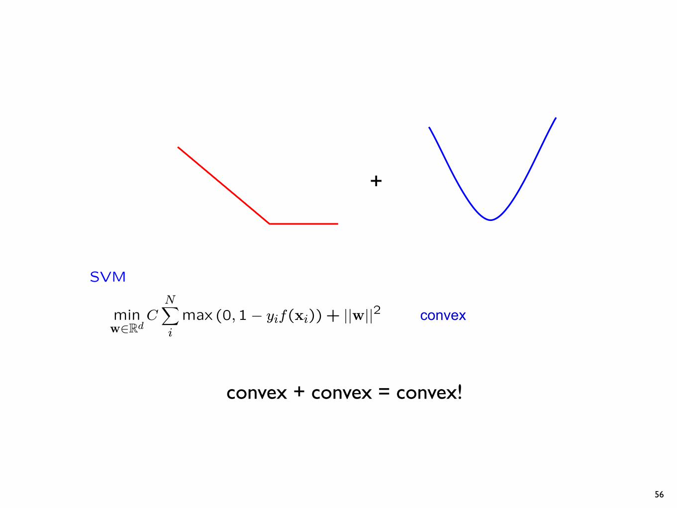
SVM
minw∈Rd
CNX
i
max (0,1− yif(xi)) + ||w||2
+
convex
56
convex + convex = convex!
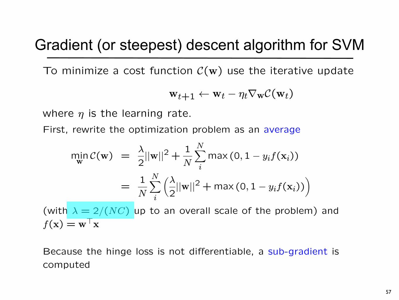
Gradient (or steepest) descent algorithm for SVM
First, rewrite the optimization problem as an average
minwC(w) =
λ
2||w||2 + 1
N
NX
i
max (0,1− yif(xi))
=1
N
NX
i
µλ
2||w||2 +max (0,1− yif(xi))
(with λ = 2/(NC) up to an overall scale of the problem) and
f(x) = w>x+ b
Because the hinge loss is not differentiable, a sub-gradient is
computed
To minimize a cost function C(w) use the iterative update
wt+1 ← wt − ηt∇wC(wt)
where η is the learning rate.
57
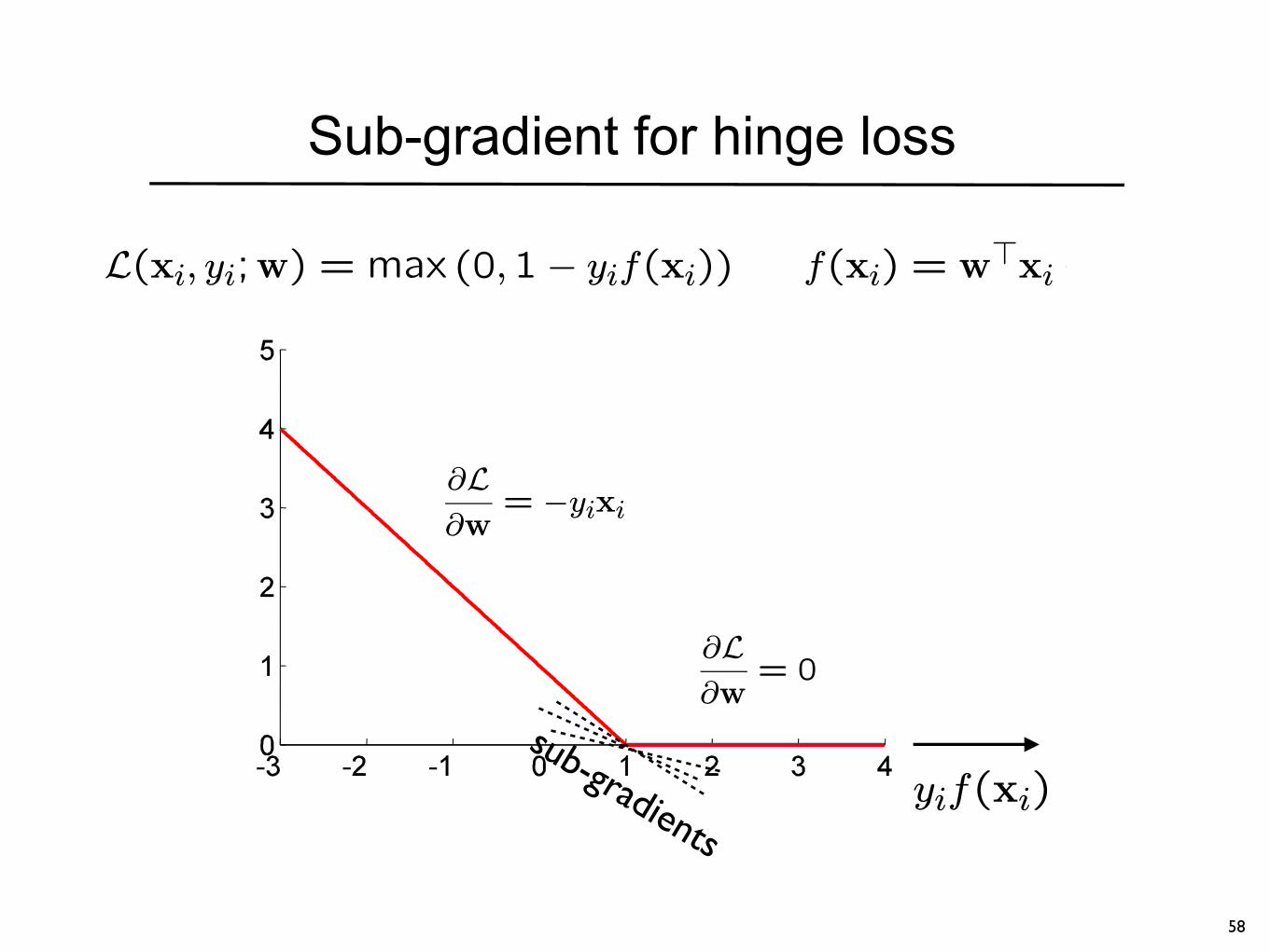
Sub-gradient for hinge loss
L(xi, yi;w) = max (0,1− yif(xi)) f(xi) = w>xi+ b
yif(xi)
∂L∂w
= −yixi
∂L∂w
= 0
58
sub-gradients
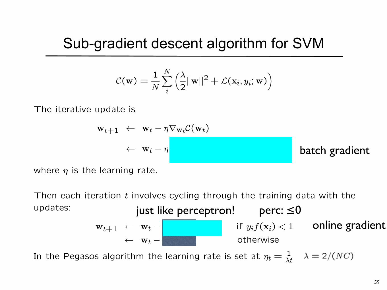
Sub-gradient descent algorithm for SVM
C(w) = 1
N
NX
i
µλ
2||w||2 + L(xi, yi;w)
The iterative update is
wt+1 ← wt − η∇wtC(wt)
← wt − η1
N
NX
i
(λwt+∇wL(xi, yi;wt))
where η is the learning rate.
Then each iteration t involves cycling through the training data with the
updates:
wt+1 ← wt − η(λwt − yixi) if yif(xi) < 1
← wt − ηλwt otherwise
In the Pegasos algorithm the learning rate is set at ηt =1λt
just like perceptron!
batch gradient
online gradient
59
perc: ≤0
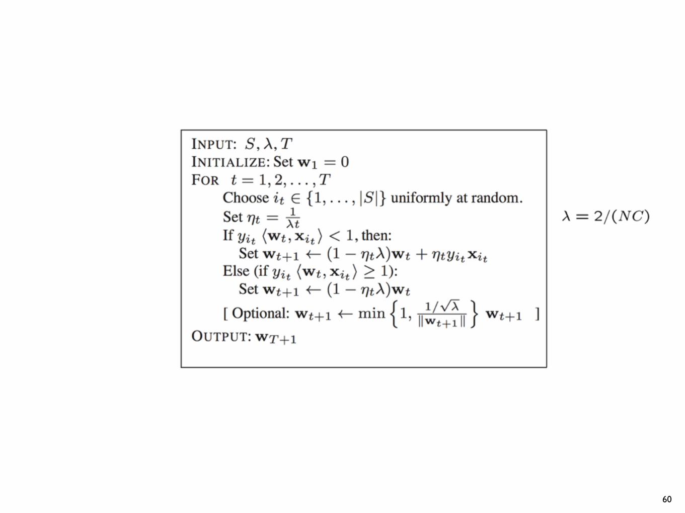
60
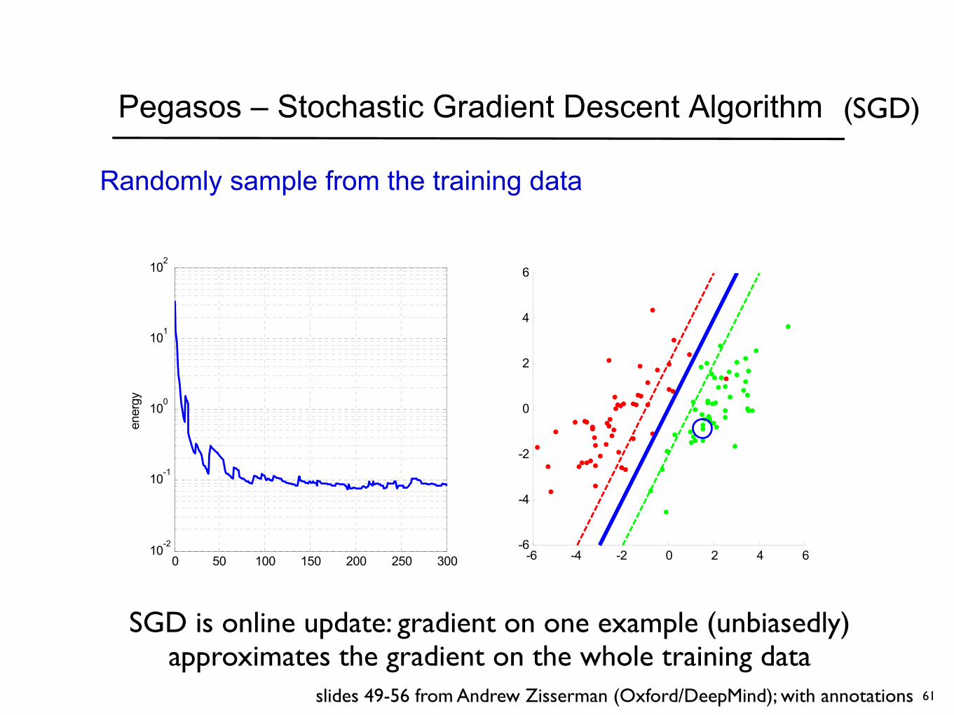
Pegasos – Stochastic Gradient Descent Algorithm
Randomly sample from the training data
0 50 100 150 200 250 30010
-2
10-1
100
101
102
ener
gy
-6 -4 -2 0 2 4 6-6
-4
-2
0
2
4
6
SGD is online update: gradient on one example (unbiasedly) approximates the gradient on the whole training data
(SGD)
61slides 49-56 from Andrew Zisserman (Oxford/DeepMind); with annotations