NASA TECHNICAL NOTE

A GEOGRAPHICAL GRID FOR NIMBUS CLOUD PICTURES

by Eqene M. Dmling, Jr.

Goddard Space Flight Center

Green belt, Maryland

SA TN D-2136

./

NATIONAL AERONAUTICS AND SPACE ADMINISTRATION l WASHINGTON, D. C. l FEBRUARY 1964 f i k I\ /

https://ntrs.nasa.gov/search.jsp?R=19640005932 2018-06-06T12:51:38+00:00Z

A GEOGRAPHICAL GRID FOR NIMBUS CLOUD PICTURES

By Eugene M. Darling, Jr.

Goddard Space Flight Center Greenbelt, Maryland

NATIONAL AERONAUTICS AND SPACE ADMINISTRATION

For sale by the Office of Technical Services, Department of Commerce, Washington, D.C. 20230 -- Price $0.50

TECH LIBRARY KAFB, NM

11#111$1!11111111ll~m~lillllll 0154392

AGEOGRAPHICALGRID FORNIMBUSCLOUD PICTURES

Eugene M. Darling, Jr.

Goddard Space Flight Center

SUMMARY

This paper defines the geometrical, -aesthetic and utilitarian factors which must be considered in selecting a geographical reference grid for use with Nimbus cloud pictures. A particular grid is proposed and critically examined with respect to these factors. This grid is found to be acceptable once minor changes are made to compensate for image foreshortening.

i

CONTENTS

Summary ................................. i

INTRODUCTION ............................ 1

GEOGRAPHIC REFERENCING ON A SPHERICAL EARTH ........................ 2

PROPERTIES OF THE NIMBUS GRID ............. 2

Constancy of Scale ........................ 2 Image Foreshortening ..................... 4 Satellite Attitude ......................... 7 Obscuration of Data ....................... 8 Aesthetics ............................. 9 Data Utilization .......................... 11 Summary and Conclusions ................... 12

References. . . . . . . . . . . . . . . . . . . . . . . . . . . . . . . . 13

. . . 111

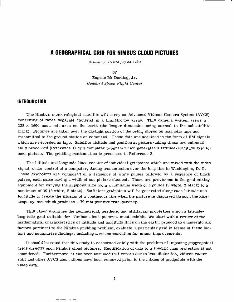
AGEOGRAPHICALGRID FORNIMBUSCLOUDPICTURES (Manuscript received July 2 2, 1963)

by Eugene M: Darling, Jr.

Goddard Space Flight Center

INTRODUCTION

The Nimbus meteorological satellite will carry an Advanced Vidicon Camera System (AVCS) consisting of three separate cameras in a trimetrogon array. This camera system views a 338 X 1600 naut. mi. area on the earth (the longer dimension being normal to the subsatellite track). Pictures are taken over the daylight portion of the orbit, stored on magnetic tape and transmitted to the ground station on command. These data are acquired in the form of FM signals which are recorded on tape. Satellite attitude and position at picture-taking times are automati- cally processed (Reference 1) by a computer program which generates a latitude-longitude grid for each picture. The gridding mathematics is presented in Reference 2.

The latitude and longitude lines consist of individual gridpoints which are mixed with the video signal, under control of a computer, during transmission over the long line to Washington, D. C. These gridpoints are composed of a sequence of white pulses followed by a sequence of black pulses, each pulse having a width of one picture element. There are provisions in the grid mixing equipment for varying the gridpoint size from a minimum width of 5 pulses (3 white, 2 black) to a maximum of 10 (5 white, 5 black). Sufficient gridpoints will be generated along each latitude and longitude to create the illusion of a continuous line when the picture is displayed through the kine- scope system which produces a ‘70 mm positive transparency.

This paper examines the geometrical, aesthetic and utilitarian properties which a latitude- longitude grid suitable for Nimbus cloud pictures must exhibit. We start with a review of the mathematical characteristics of latitude and longitude lines on the earth, proceed to enumerate six factors pertinent to the Nimbus gridding problem; evaluate a particular grid in terms of these fac- tors and summarize findings, including a recommendation for minor improvements.

It should be noted that this study is concerned solely with the problem of imposing geographical grids directly upon Nimbus cloud pictures. Rectification of data to a specific map projection is not considered. Furthermore, it has been assumed that errors due to lens distortion, vidicon raster shift and other AVCS aberrations have been removed prior to the mixing of gridpoints with the video data.

1

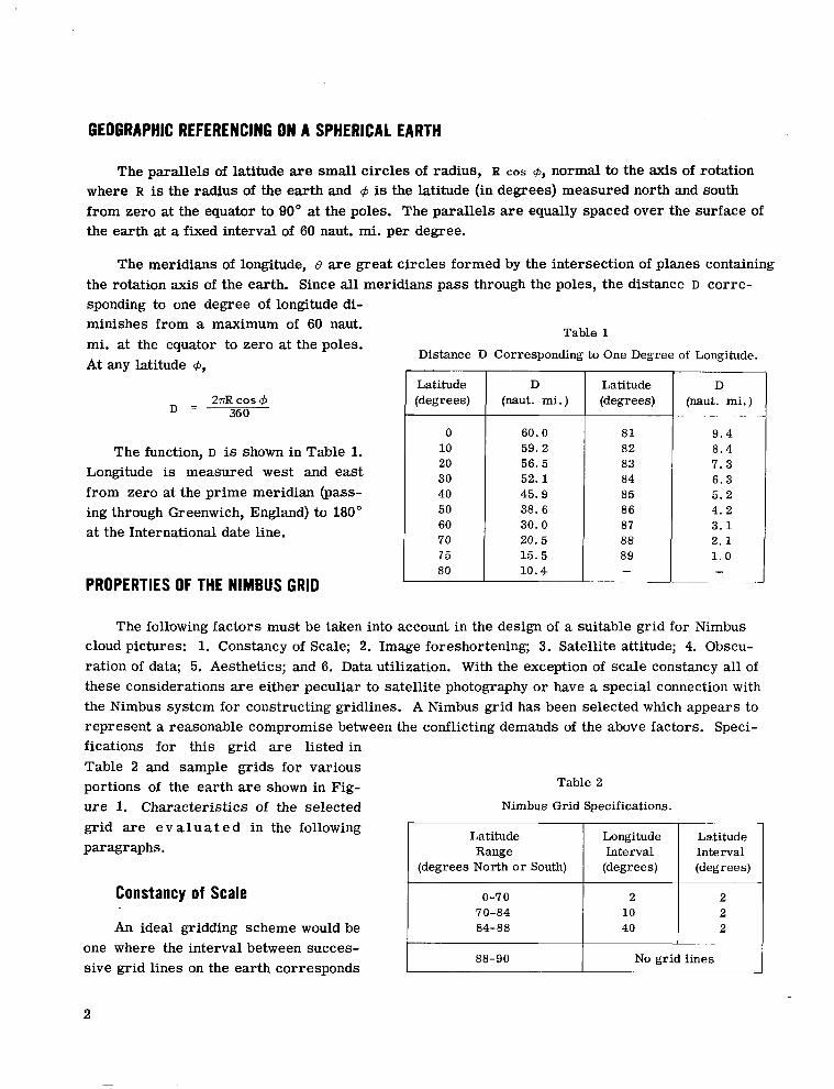
GEOGRAPHIC REFERENClNG ON A SPHERICAL EARTH

The parallels of latitude are small circles of radius, R cos 4, normal to the axis of rotation where R is the radius of the earth and 4 is the latitude (in degrees) measured north and south from zero at the equator to 90’ at the poles. The parallels are equally spaced over the surface of the earth at a fixed interval of 60 naut. mi. per degree.

The meridians of longitude, e are great circles formed by the intersection of planes containing the rotation axis of the earth. Since all meridians pass through the poles, the distance D corre- sponding to one degree of longitude di- minishes from a maximum of 60 naut. mi. at the equator to zero at the poles. At any latitude 6,

D = 2nR cos 4

360

The function, D is shown in Table 1. Longitude is measured west and east from zero at the prime meridian (pass- ing through Greenwich, England) to 180” at the International date line.

PROPERTIESOFTHE NIMBUS GRID

Table 1

Distance D Corresponding to One Degree of Longitude.

Latitude (degrees)

0 10 20 30 40 50 60 70 75 80 :

D (naut. mi.)

60.0 59.2 56.5 52.1 45.9 38.6 30.0 20.5 15.5 10.4

Latitude (degrees)

81 82 83 84 85 86 87 88 89 -

1

:

D (naut. mi.)

9.4 8.4 7.3 6.3 5.2 4.2 3.1 2.1 1.0

The following factors must be taken into account in the design of a suitable grid for Nimbus cloud pictures: 1. Constancy of Scale; 2. Image foreshortening; 3. Satellite attitude; 4. Obscu- ration of data; 5. Aesthetics; and 6. Data utilization. With the exception of scale constancy all of these considerations are either peculiar to satellite photography or have a special connection with the Nimbus system for constructing gridlines. A Nimbus grid has been selected which appears to represent a reasonable compromise between the conflicting demands of the above factors. Speci- fications for this grid are listed in Table 2 and sample grids for various portions of the earth are shown in Fig- Table 2

ure 1. Characteristics of the selected Nimbus Grid Specifications.

grid are evaluated in the following Latitude

paragraphs. Range (degrees North or South)

Constancy of Scale 70-84

An ideal gridding scheme would be one where the interval between succes- sive grid lines on the earth corresponds

Longitude Interval

(degrees)

2 10 40

Latitude Interval (degrees)

2 2 2

No grid lines

1

2

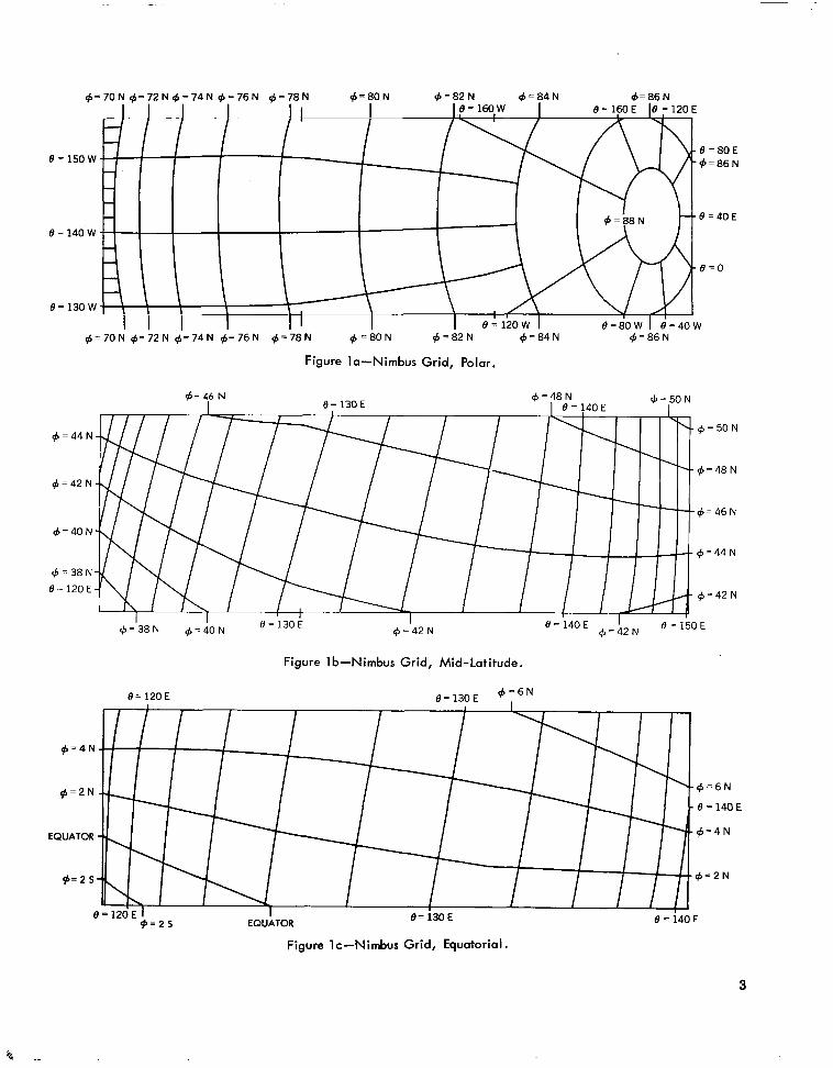
$=7ON +=72N .$=74N +=76N $=78N

Figure la-Nimbus Grid, Polar.

d=415N _ _-_- +=48N d~=!iflN I tl=1mt 1 ~9=140E

, --.. I

I

+=44N- L-+=50N

\

‘\-+=48N

~=40N~~~~+~+=46N

+=42N

+ =‘38 N t#,=dON O= 130E 4 =‘42 N 0=140E 0=150E

Figure 1 b-Nimbus Grid, Mid-Latitude.

O= 120E O= 130E $fB=bN

-B=140E

EQUATOR O= 130 E 8=14OF

Figure lc-Nimbus Grid, Equatorial.

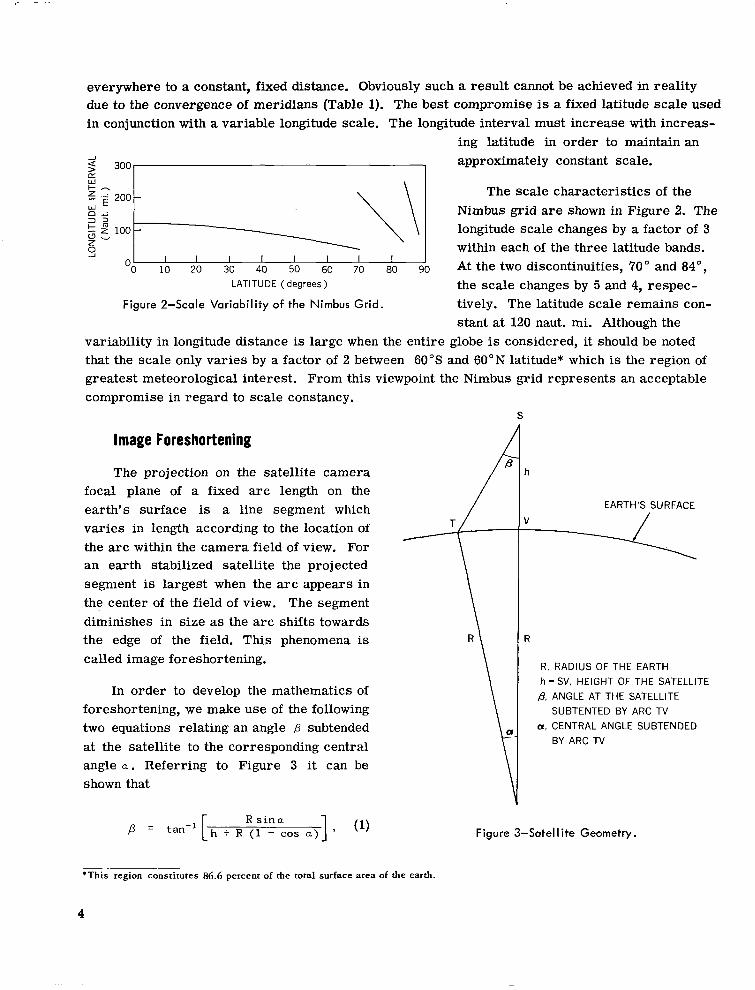
everywhere to a constant, fixed distance. Obviously such a result cannot be achieved in reality due to the convergence of meridians (Table 1). The best compromise is a fixed latitude scale used in conjunction with a variable longitude scale. The longitude interval must increase with increas-

ing latitude in order to maintain an

2 2

300 approximately constant scale.

z ; 200 - The scale characteristics of the

0”; 2 5 loo-

\\\

Nimbus grid are shown in Figure 2. The

is- longitude scale changes by a factor of 3

9 within each of the three latitude bands. I I I I I I

‘0 10 20 30 40 50 60 70 80 90 At the two discontinuities, 70” and 84”, LATITUDE ( degrees ) the scale changes by 5 and 4, respec-

Figure 2-Scale Variability of the Nimbus Grid. tively. The latitude scale remains con- stant at 120 naut. mi. Although the

variability in longitude distance is large when the entire globe is considered, it should be noted that the scale only varies by a factor of 2 between 60”s and 60”N latitude* which is the region of greatest meteorological interest. From this viewpoint the Nimbus grid represents an acceptable compromise in regard to scale constancy.

S

Image Foreshortening

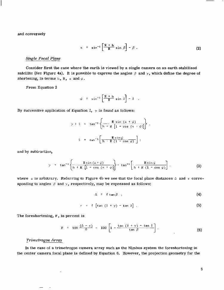
The projection on the satellite camera focal plane of a fixed arc length on the earth’s surface is a line segment which varies in length according to the location of the arc within the camera field of view. For an earth stabilized satellite the projected segment is largest when the arc appears in th” center of the field of view. The segment diminishes in size as the arc shifts towards the edge of the field. This phenomena is called image foreshortening.

In order to develop the mathematics of foreshortening, we make use of the following two equations relating an angle p subtended at the satellite to the corresponding central angle a. Referring to Figure 3 it can be shown that

p = tan-l R sina 1 h+R(l-cosa) ’ (1)

h

EARTH’S SURFACE

R

R, RADIUS OF THE EARTH

h = SV, HEIGHT OF THE SATELLITE

,8, ANGLE AT THE SATELLITE

SUBTENTED BY ARC TV

a, CENTRAL ANGLE SUBTENDED

BY ARC TV

Figure 3-Sate1 I ite Geometry,

*This region constitutes 866 percent of the total surface area of the earth.

4

and conversely

R+h a = sin-’ R sinp -p. 1 (2)

Single Focal Plane

Consider first the case where the earth is viewed by a single camera on an earth stabilized satellite (See Figure 4a). It is possible to express the angles p and y, which define the degree of shortening, in terms h, R, CL and #.

From Equation 2

4 = si”-l !p [

sin 6 1 -6 . By successive application of Equation 1, y is found as follows:

yts = R sin (a f $J)

h + R [l - cos (a + #)] ’

s = tan -1 h+R(l-cos$) ; 1

and by subtraction,

Y = tan-l Rsin$

h + R [l - cos (a + 1 h+R(l-costi) ’ (3)

where a is arbitrary. Referring to Figure 4b we see that the focal plane distances A and E corre- sponding to angles p and y, respectively, may be expressed as follows:

A q f tan,B ; (4)

E = f [tan(S+y)-tan&]. (5)

The foreshortening, F, in percent is

F = (A-E) =

100 7 I. (6)

Trim e trogon Array

In the case of a trimetrogon camera array such as the Nimbus system the foreshortening in the center camera focal plane is defined by Equation 6. However, the projection geometry for the

5

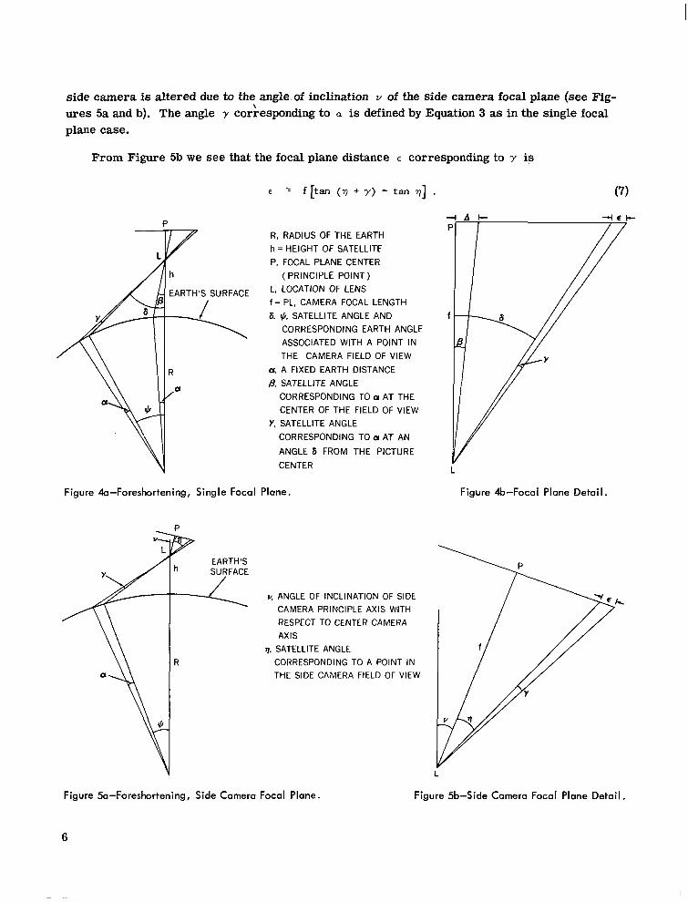
side camera is altered due to the angle of inclination v of the side camera focal plane (see Fig- ures 5a and b). The angle y corkesponding to a is defined by Equation 3 as in the single focal plane case.

From Figure 5b we see that the focal plane distance c corresponding to y is

E : f [tan (7 + y) - tan 7)]

R, RADIUS OF THE EARTH

h = HEIGHT OF SATELLITE

P. FOCAL PLANE CENTER

(PRINCIPLE POINT)

L. LOCATION OF LENS

f = PL. CAMERA FOCAL LENGTH

8, +b, SATELLITE ANGLE AND

CORRESPONDING EARTH ANGLE

ASSOCIATED WITH A POINT IN

THE CAMERA FIELD OF VIEW

u, A FIXED EARTH DISTANCE

/j SATELLITE ANGLE

CORRESPONDING TO u AT THE

CENTER OF THE FIELD OF VIEW

Y, SATELLITE ANGLE

CORRESPONDING TO a AT AN

ANGLE 6 FROM THE PICTURE

CENTER

Figure 4a-Foreshortening, Single Focal Plane. Figure 4b-Focal Plane Detail.

EARTH’S SURFACE

2 v, ANGLE OF INCLINATION OF SIDE

CAMERA PRINCIPLE AXIS WITH

RESPECT TO CENTER CAMERA

AXIS

q, SATELLITE ANGLE

R CORRESPONDING TO A POINT IN

THE SIDE CAMERA FIELD OF VIEW

Figure 5b-Side Camera Focal Plane Detail. Figure 5a-Foreshortening, Side Camera Focal Plane.

6

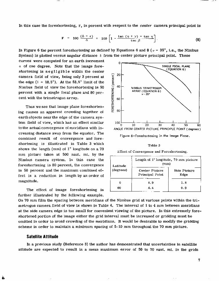
In this case the foreshortening, F, in percent with respect to the center camera principal point is

F = 1oo CA ; ‘) = tan (7) + r> - tan “1. 100 1 - [ tan /3 03)

In Figure 6 the percent foreshortening as defined by Equations 6 and 8 (V = 35”, i.e., the Nimbus System) is plotted versus angular distance 6 from the center picture principal point. These curves were computed for an earth increment a of one degree. Note that the image fore- shortening is ne gli gib 1 e within the center camera field of view, being only 3 percent at the edge (6 = 18.5”). At the 53.5” limit of the Nimbus field of view the foreshortening is 50 percent with a single focal plane and 80 per- cent with the trimetrogon array.

Thus we see that image plane foreshorten- ing causes an apparent crowding together of earthobjects near the edge of the camera sys- tem field of view, which has an effect similar to the actual convergence of meridians with in- creasing distance away from the equator. The combined result of convergence and fore- shortening is illustrated in Table 3 which shows the length (mm) of 1” longitude on a ‘70 mm picture taken at 500 naut. mi. by the Nimbus camera system. In this case the foreshortening is 80 percent, the convergence is 50 percent and the maximum combined ef- fect is a reduction in length by an order of magnitude.

The effect of image foreshortening is further illustrated by the following example.

o- SINGLE FOCAL PLANE

z 20- : 2 8 - 40- P z

ARRAY ( EQUATION 8)

e lJ=35"

g 60-

5 E 2 80-

1ool I I I I I _- 0 10 20 30 40 50 60

ANGLE FROM CENTER PICTURE PRINCIPLE POINT (degrees)

Figure 6-Foreshortening in the Image Plane.

Table 3

Effect of Convergence and Foreshortening.

I Length of 1” longitude, 7 0 mm picture

Latitude _ (mm)

(degrees) Center Picture Side Picture Principal Point Edge

0 8.9 1.8

60 4.4 0.9

On 70 mm film the spacing between meridians of the Nimbus grid at various points within the tri- metrogon camera field of view is shown in Table 4. The interval of 1 to 4 mm between meridians at the side camera edge is too small for convenient viewing of the picture. In this extremely fore- shortened portion of the image either the grid interval must be increased or gridding must be omitted in order to avoid crowding of the meridians. It would be desirable to modify the gridding scheme in order to maintain a minimum spacing of 5-10 mm throughout the 70 mm picture.

Satellite Attitude

In a previous study (Reference 3) the author has demonstrated that uncertainties in satellite attitude are expected to result in a mean maximum error of 50 to 70 naut. mi. in the grids

7

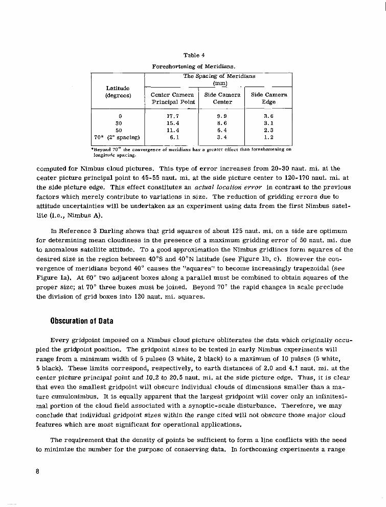
Table 4

1

Foreshortening of Meridians. ___-~

The Spacing of Meridians

I Latitude m-4

I I

I (degrees) Center Camera Side Camera Side Camera Principal Point Center Edge

0 17.7 9.9 3.6 30 15.4 6.6 3.1 50 11.4 6.4 2.3

70* (2’ spacing) 6.1 3.4 1.2

‘Beyond 70” the coovergence of meridians has a greater effect than foreshortening on longitude spacing.

computed for Nimbus cloud pictures. This type of error increases from 20-30 naut. mi. at the center picture principal point to 45-55 naut. mi. at the side picture center to 120-170 naut. mi. at the side picture edge. This effect constitutes an actual location. eyyoy in contrast to the previous factors which merely contribute to variations in size. The reduction of gridding errors due to attitude uncertainties will be undertaken as an experiment using data from the first Nimbus satel- lite (i.e., Nimbus A).

In Reference 3 Darling shows that grid squares of about 125 naut. mi. on a side are optimum for determining mean cloudiness in the presence of a maximum gridding error of 50 naut. mi. due to anomalous satellite attitude. To a good approximation the Nimbus gridlines form squares of the desired size in the region between 40”s and 40”N latitude (see Figure lb, c). However the con- vergence of meridians beyond 40” causes the “squares” to become increasingly trapezoidal (see Figure la). At 60” two adjacent boxes along a parallel must be combined to obtain squares of the proper size; at 70” three boxes must be joined. Beyond 70” the rapid changes in scale preclude the division of grid boxes into 120 naut. mi. squares.

Obscuration of Data

Every gridpoint imposed on a Nimbus cloud picture obliterates the data which originally occu- pied the gridpoint position. The gridpoint sizes to be tested in early Nimbus experiments will range from a minimum width of 5 pulses (3 white, 2 black) to a maximum of 10 pulses (5 white, 5 black). These limits correspond, respectively, to earth distances of 2.0 and 4.1 naut. mi. at the center picture principal point and 10.2 to 20.5 naut. mi. at the side picture edge. Thus, it is clear that even the smallest gridpoint will obscure individual clouds of dimensions smaller than a ma- ture cumulonimbus. It is equally apparent that the largest gridpoint will cover only an infinitesi- mal portion of the cloud field associated with a synoptic-scale disturbance. Therefore, we may conclude that individual gridpoint sizes within the range cited will not obscure those major cloud features which are most significant for operational applications.

The requirement that the density of points be sufficient to form a line conflicts with the need to minimize the number for the purpose of conserving data. In forthcoming experiments a range

8

of gridpoint sizes and point densities along grid lines will be examined for readability and suita- bility. The following maximum sizes will be associated with the densities indicated:

Maximum Gridpoint Size Density

5 elements ; 1 point/l5 elements 10 elements; 1 point/30 elements

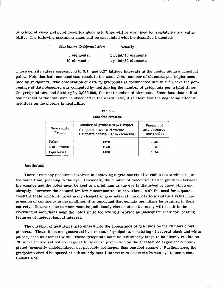
These density values correspond to 0.1” and 0.2” latitude intervals at the center picture principal point. Note that both combinations result in the same total number of elements per triplet occu- pied by gridpoints. The obscuration of data by gridpoints is documented in Table 5 where the per- centage of data obscured was computed by multiplying the number of gridpoints per triplet times the gridpoint size and dividing by 2,085,000, the total number of elements. Since less than half of one percent of the total data is obscured in the worst case, it is clear that the degrading effect of gridlines on the picture is negligible.

Table 5

Data Obscuration.

Aesthetics

Geographic Region

Polar Mid Latitude Equatorial

Number of gridpoints per triplet Percent of Gridpoint size: 5 elements data obscured Gridpoint density: l/15 elements per triplet

1570 0.38 1930 0.46 1430 0.34

There are many problems involved in achieving a grid matrix of variable scale which is, at the same time, pleasing to the eye. Obviously, the number of discontinuities in gridlines between the equator and the poles must be kept to a minimum as the eye is disturbed by lines which end abruptly. However the demand for few discontinuities is at variance with the need for a quasi- constant scale which requires many changes in grid interval. In order to maintain a visual im- pression of continuity in the gridlines it is important that certain meridians be retained in their entirety. However, the number must be judiciously chosen since too many will result in the crowding of meridians near the poles while too few will provide an inadequate scale for locating features of meteorological interest.

The question of aesthetics also enters into the appearance of gridlines on the Nimbus cloud pictures. These lines are generated by a series of gridpoints consisting of several black and white pulses, each an element wide. These gridpoints must be sufficiently large to be clearly visible on 70 mm film and yet not so large as to be out of proportion on the greatest enlargement contem- plated (presently undetermined, but probably not larger than one foot square). Furthermore, the gridpoints should be spaced at sufficiently small intervals to cause the human eye to see a con- tinuous line.

9

The appearance of the Nimbus grid will be generally pleasing to the eye. Visual continuity over the globe is achieved by retaining nine meridians in their entirety from the equator to the poles. Scale discontinuities have been kept to the irreducible number of two, both of which occur poleward of the Arctic Circle (i.e., at 70” and 84”). Thus there is no change in scale over the major continental areas of the world.

The width of a gridline varies as a function of orientation with respect to raster lines. This is another factor which affects the aesthetic quality of the grid. If B is the angle between a raster line and a gridline consisting of gridpoints of e elements iength, then the width w of the gridline is

W = i? sin B for e > 0

Z r for L9 = 0

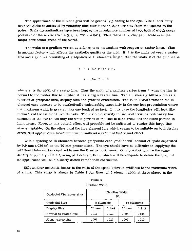
where r is the width of a raster line. Thus the width of a gridline varies from P when the line is normal to the raster line to r when it lies along a raster line. Table 6 shows gridline width as a function of gridpoint size, display size and gridline orientation. The 10 to 1 width ratio in the 10 element case appears to be aesthetically undesirable, especially in the one foot presentation where the maximum width is greater than one tenth of an inch. In this case the longitudes will look like ribbons and the latitudes like threads. The visible disparity in line width will be reduced by the tendency of the eye to see only the white portion of the line in dark areas and the black portion in light areas. However this optical effect will probably not be sufficient to render this large line size acceptable. On the other hand the five element line which seems to be suitable on both display sizes, will appear even more uniform in width as a result of this visual effect.

With a spacing of 15 elements between gridpoints each gridline will consist of spots separated by 0.9 mm (.036 in) on the 70 mm presentation. The eye should have no difficulty in supplying the additional information required to see the lines as continuous. On a one foot picture the same density of points yields a spacing of 1 every 0.15 in. which will be adequate to define the line, but its appearance will be distinctly dotted rather than continuous.

Still another aesthetic factor is the ratio of the space between gridlines to the maximum width of a line. This ratio is shown in Table 7 for lines of 5 element width at three places in the

,

Table 6

Gridline Width. I

Gridpoint Characteristics Gridline Width

On) -. -- Gridpoint Size 5 elements 10 elements

.~ Display Size 70 mm 1 foot 70 mm 1 foot

Normal to raster line .012 .051 .024 .103

Along raster line .002 .OlO .002 .OlO

10

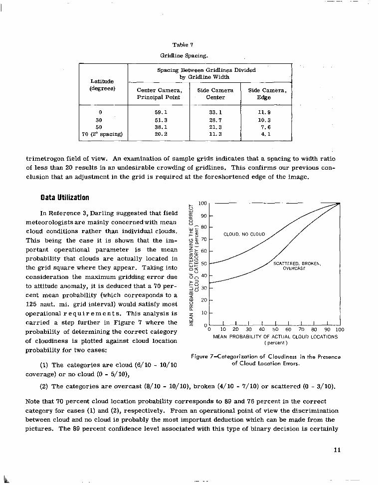
Table 7

Gridline Spacing.

Spacing Between Gridlines Divided

Latitude by Gridline Width

(degrees) Center Camera, Side Camera Side Camera, Principal Point Center E&e

0 59.1 33.1 11.9 30 51.3 28.7 10.3 50 38.1 21.3 7.6

70 (2" spacing) 20.2 11.3 4.1

trimetrogon field of view. An examination of sample grids indicates that a spacing to width ratio of less than 20 results in an undesirable crowding of gridlines. This confirms our previous con- clusion that an adjustment in the grid is required at the foreshortened edge of the image.

Data Utilization

In Reference 3, Darling suggested that field meteorologists are mainly concerned with mean cloud conditions rather than individual clouds. This being the case it is shown that the im- portant operational parameter is the mean probability that clouds are actually located in the grid square where they appear. Taking into consideration the maximum gridding error due to attitude anomaly, it is deduced that a 70 per- cent mean probability (which corresponds to a 125 naut. mi. grid interval) would satisfy most operational r e q u i r e m e n t s. This analysis is carried a step further in Figure 7 where the probability of determining the correct category of cloudiness is plotted against cloud location probability for two cases:

(1) The categories are cloud (6/10 - lO/lO coverage) or no cloud (0 - 5/10),

2 o! I I I I I I I I I 0 10 20 30 40 50 60 70 80 90 100

MEAN PROBABILITY OF ACTUAL CLOUD LOCATIONS ( percent )

Figure 7-Categorization of Cloudiness in the Presence of Cloud Location Errors.

(2) The categories are overcast (8/10 - lo/lo), broken (4/10 - 7/10) or scattered (0 - 3/10).

Note that 70 percent cloud location probability corresponds to 89 and 76 percent in the correct category for cases (1) and (2), respectively. From an operational point of view the discrimination between cloud and no cloud is probably the most important deduction which can be made from the pictures. The 89 percent confidence level associated with this type of binary decision is certainly

11

adequate. Since this high confidence level corresponds to the maximum gridding error anticipated, we may conclude that the previously deduced 70 percent cloud location probability and attendant 125 naut. mi. grid interval are supported by this analysis.

We have indicated that the Nimbus grid is adequate to determine mean cloudiness in grid squares 120 naut. mi. on a side, between 70”s andC 70”N latitude, even in the case of maximum satellite attitude deviation from nominal. In fact the grid was specifically designed for this pur- pose. The grid is less adaptable to the location of individual cloud features due to the long dis- tances over which interpolation must be performed.

The error to be expected in locating individual features may be estimated by making the fol- lowing assumptions about the accuracy of interpolation as a function of grid spacing:

On 70 mm film the error due to interpolation is l/10 the distance between gridlines for spacings > 10 mm; l/5 for spacings of 3 to < 10 mm; l/2 for < 3 mm.

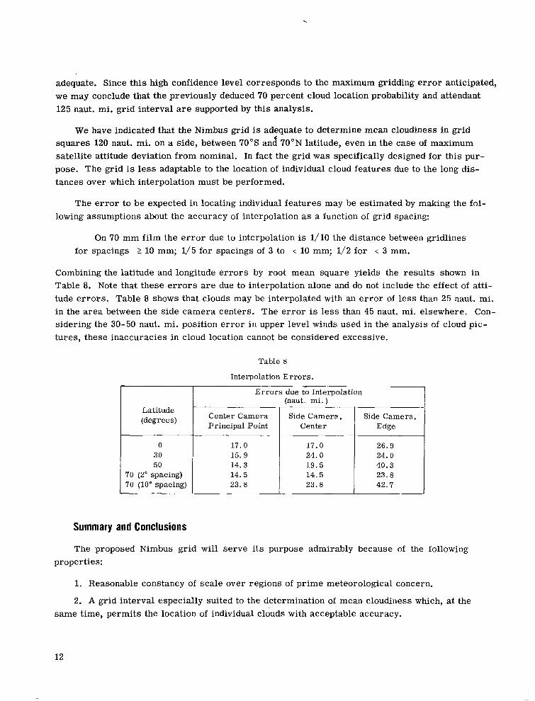
Combining the latitude and longitude errors by root mean square yields the results shown in Table 8. Note that these errors are due to interpolation alone and do not include the effect of atti- tude errors. Table 8 shows that clouds may be interpolated with an error of less than 25 naut. mi. in the area between the side camera centers. The error is less than 45 naut. mi. elsewhere. Con- sidering the 30-50 naut. mi. position error in upper level winds used in the analysis of cloud pic- tures, these inaccuracies in cloud location cannot be considered excessive.

70 (2” spacing)

T

Table 8

Interpolation Errors.

Errors due to Interpolation1

Center Camera Principal Point

17.0 15.9 14.3 14.5 23. 8

(naut. mi. ) -

Side Camera, Side Camera, Center Edge

17.0 26.9 24.0 24.0 19.5 40.3 14.5 23.8 23.8 42.7

Summary and Conclusions

The proposed Nimbus grid will serve its purpose admirably because of the following properties:

1. Reasonable constancy of scale over regions of prime meteorological concern.

2. A grid interval especially suited to the determination of mean cloudiness which, at the same time, permits the location of individual clouds with acceptable accuracy.

12

3. Negligible obscuration of data by gridlines.

4. A pleasing balance of line width and spacing over most of the three picture area.

A slight alteration of the grid interval is required in the extremely foreshortened edges of the side pictures in order to avoid crowding of meridians.

REFERENCES

1. “Nimbus Command and Data Acquisition (CDA) Station Data System Performance Requirements and Equipment Interface Specifications,” General Electric Document No. 63SD557, Revision A, May 30, 1963 (Contract NAS 5-3116).

2. “Operational Gridding Methods for the Nimbus Vidicon System,” by R. DeBiase, et al. General Electric Document No. 63SD770, June 6, 1963 (Contract NAS 5-3116).

3. “An Analysis of Errors in the Geographic Referencing of Nimbus Cloud Pictures,” by E. M. Darling, Jr. NASA Technical Note D-2137, 1963 (In Press).

NASA-Langley, 1964 G-473 13