A Generative Model of Urban Activities from Cellular Data · A Generative Model of Urban Activities from Cellular Data by Mogeng Yin Master of Science in Electrical Engineering and

A Generative Model of Urban Activities from Cellular Data

Mogeng YinMadeleine SheehanSidney FeyginJean-Francois PaiementAlexei PozdnoukhovAlexandre Bayen

Electrical Engineering and Computer SciencesUniversity of California at Berkeley

Technical Report No. UCB/EECS-2017-201http://www2.eecs.berkeley.edu/Pubs/TechRpts/2017/EECS-2017-201.html

December 12, 2017

Copyright © 2017, by the author(s).All rights reserved.

Permission to make digital or hard copies of all or part of this work forpersonal or classroom use is granted without fee provided that copies arenot made or distributed for profit or commercial advantage and that copiesbear this notice and the full citation on the first page. To copy otherwise, torepublish, to post on servers or to redistribute to lists, requires prior specificpermission.

Acknowledgement

I would like to thank my advisor in the EECS department Alexandre Bayenfor his caring, support and advice in my research and life. I would like tothank my advisor in my home department Alexei Pozdnoukhov for hissupport and sponsorship, without whom I stand no chance studying in theEECS department and work on such an interesting research problem. Iwould also like to thank my advisor at AT&T labs research Jean-FrancoisPaiement for his support and priceless guidance on my research. I would liketo thank Professor Randy Katz for reviewing and providing valuablecomments on the report.


by

Mogeng Yin

A dissertation submitted in partial satisfaction of the

requirements for the degree of

Master of Science

in

Electrical Engineering and Computer Sciences

in the

Graduate Division

of the

University of California, Berkeley

Committee in charge:

Professor Alexandre M. Bayen, Chair

Fall 2017


Copyright 2017by

Mogeng Yin

1

Abstract


by

Mogeng Yin

Master of Science in Electrical Engineering and Computer Sciences

University of California, Berkeley

Professor Alexandre M. Bayen, Chair

Activity based travel demand models are becoming essential tools used in transportationplanning and regional development scenario evaluation. They describe travel itineraries ofindividual travelers, namely what activities they are participating in, when they performthese activities, and how they choose to travel to the activity locales. However, data col-lection for activity based models is performed through travel surveys that are infrequent,expensive, and reflect the changes in transportation with significant delays. Thanks to theubiquitous cell phone data, we see an opportunity to substantially complement these surveyswith data extracted from network carrier mobile phone usage logs, such as call detail records(CDRs). In this paper, we develop Input-Output Hidden Markov Models (IO-HMMs) toinfer travelers’ activity patterns from CDRs. We apply the model to the data collected by amajor network carrier serving millions of users in the San Francisco Bay Area. Our approachdelivers an end-to-end actionable solution to the practitioners in the form of a modular andinterpretable activity-based travel demand model. It is experimentally validated with threeindependent data sources: aggregated statistics from travel surveys, a set of collected groundtruth activities, and the results of a traffic micro-simulation informed with the travel planssynthesized from the developed generative model.

i

Contents

Contents i

List of Figures ii

List of Tables iv

1 Introduction 1

2 Related Work 32.1 Locational Data Sources . . . . . . . . . . . . . . . . . . . . . . . . . . . . . 32.2 Methods and Approaches . . . . . . . . . . . . . . . . . . . . . . . . . . . . . 4

3 Modeling Framework 6

4 Activity Recognition and Generation 94.1 IO-HMM for Activity Pattern Recognition . . . . . . . . . . . . . . . . . . . 94.2 Model Specification . . . . . . . . . . . . . . . . . . . . . . . . . . . . . . . . 124.3 Model Selection . . . . . . . . . . . . . . . . . . . . . . . . . . . . . . . . . . 144.4 Activity Chains Generation . . . . . . . . . . . . . . . . . . . . . . . . . . . 16

5 Experimental Results 175.1 Data Pre-processing . . . . . . . . . . . . . . . . . . . . . . . . . . . . . . . 175.2 Activity Recognition Results . . . . . . . . . . . . . . . . . . . . . . . . . . . 185.3 Evaluation of Activity Recognition . . . . . . . . . . . . . . . . . . . . . . . 235.4 Activity Generation from an IO-HMM . . . . . . . . . . . . . . . . . . . . . 255.5 Evaluation via Traffic Micro-simulation . . . . . . . . . . . . . . . . . . . . . 27

6 Conclusion and Future Work 30

A Stay points detection in CDR 32

B Home and Work Inference 34

Bibliography 35

ii

List of Figures

3.1 Modeling framework diagram. The left column represents the input to the re-search; the middle column represents the key modeling components; and the rightcolumn represents the products of the research. Our key contribution of activityrecognition and generation module are outlined with the red dashed rectangle,and the key components are shown in shaded yellow. . . . . . . . . . . . . . . . 7

3.2 Call Detail Records (CDR) data processing. The table at left represents theraw CDR format, i.e., time stamped record of communications. A stay pointsdetection algorithm (detailed in Appendix A) is used to convert the raw CDRdata to a sequence of stay locations with start time, duration and location ID, asrepresented in the table at right. . . . . . . . . . . . . . . . . . . . . . . . . . . 8

4.1 IO-HMM Architecture. The solid nodes represent observed information, whilethe transparent (white) nodes represent latent random variables. The top layercontains the observed input variables ut; the middle layer contains latent cat-egorical variables zt; and the bottom layer contains observed output variablesxt. . . . . . . . . . . . . . . . . . . . . . . . . . . . . . . . . . . . . . . . . . . . 10

4.2 Structural patterns of empirical data collected at short range DASs well explainthe activity performed around the DASs: the number of activities start timeswithin a course of a week (left) and an empirical joint distribution plot of thevisit duration versus start times (right). . . . . . . . . . . . . . . . . . . . . . . 15

5.1 Empirical distributions of the average number of daily activities of San Franciscosubscribers on a weekday (left) and on a weekend (right), after pre-processing. . 18

5.2 Density map of inferred home and work locations for San Francisco residents,aggregated at the census tract level (left), and an overall geographical scope ofanalysis with work locations density (right). . . . . . . . . . . . . . . . . . . . . 19

5.3 Number of activities (labeled per highest posterior probability) by their respectivestart time within a course of a week. . . . . . . . . . . . . . . . . . . . . . . . . 20

5.4 Joint distribution plot of duration and start hour per activity type. The labels aregained by assigning the activity to the one with the highest posterior probabilityafter training. . . . . . . . . . . . . . . . . . . . . . . . . . . . . . . . . . . . . . 22

5.5 Heterogeneous activity transition matrices under different contextual variables. . 23

iii

5.6 Distribution of activity start times over a course of a day of four example commonactivity patterns generated from the Bay Area IO-HMMs. Note that all simulatedactivitity patterns start at home, so (a) designates the Home-Work-Home travelpattern. The x-axis designates the start time of the activity, the y-axis representsthe proportion of trips (for users with this activity pattern) starting at this time. 27

5.7 A fragment of the SF Bay Area road network with the location of 600 trafficvolume detectors used for validation (shown with small black dots). Inlet graphsillustrate three sample hourly vehicle volume profiles for observed (orange) andmodeled (blue) flows on a typical weekday in Summer 2015. . . . . . . . . . . . 28

5.8 Micro-simulation validation with the observed freeway traffic volumes . . . . . . 29

iv

List of Tables

4.1 Highlights of comparison between an HMM versus. IO-HMM (ut, zt, xt denoteinput, hidden and output variables respectively, i is an index of a hidden state, tis a sequence timestamp index). . . . . . . . . . . . . . . . . . . . . . . . . . . . 11

4.2 Rules of labeling secondary activities based on activity spatial-temporal features 16

5.1 Model coefficients for the output variables per hidden activity (see interpretationin the text). . . . . . . . . . . . . . . . . . . . . . . . . . . . . . . . . . . . . . . 19

5.2 Confusion matrix of inferred activities versus “ground truth” activities . . . . . 245.3 Comparison of model accuracy . . . . . . . . . . . . . . . . . . . . . . . . . . . 24

v

Acknowledgments

I would like to thank my advisor in the EECS department Alexandre Bayen for his caring,support and advice in my research and life. I would like to thank my advisor in my homedepartment Alexei Pozdnoukhov for his support and sponsorship, without whom I stand nochance studying in the EECS department and work on such an interesting research problem.I would also like to thank my advisor at AT&T labs research Jean-Francois Paiement for hissupport and priceless guidance on my research.

1

Chapter 1

Introduction

Novel mobility paradigms change the transportation landscape quicker than traditional datasources, such as travel surveys, are able to reflect. A vital example is on-demand trans-portation enabled by a range of services connecting drivers with potential passengers. Thisincreased flexibility of travel options manifests itself in the way citizens structure their day,and causes significant shifts in urban mobility patterns. Public agencies charged with a man-date to manage critical transportation infrastructures are slow to react to these changes, asthey are reliant on out-dated information, tools, and models. Part of the problem is thereliance of their methodologies on manually conducted travel surveys.

The National Household Travel Survey (NHTS), the data source that is typically thecrux of travel demand models, is conducted every 5 years, and carries a total cost of millionsof dollars [18]. NHTS is further limiting because a typical survey only covers two percent ofhouseholds in a metropolitan area, and typically only records one day of travel per household[32].

At the same time, people generate data while traveling by carrying and using a mobilephone. A valuable alternative is to use a non-invasive, automated, continuous data collectionmechanism to complement, supplement, and augment manual surveying. The main advan-tages are 3-fold: (1) it vastly increases sample size; (2) it eliminates the delays normallyassociated with administering and processing travel surveys; and (3) it improves activity-based travel modeling by taking advantage of spatially and temporally rich cell phone traces,which capture users activities over months, rather than a single day. While studies of mo-bility from crowd-sourced locational data are common (these are thoroughly reviewed inSection 2), no existing work provides models in the form that transportation practitionersactually require.

Typical activity-based travel models used by practitioners are incredibly rich in describingthe intricacies of human activities and context of decision making in travel-related choices.For years, discrete choice models of travel included trip purpose as context [4]. It is a signif-icant factor influencing decisions on mode and other attributes of travel. One key researchchallenge therefore lies in detecting trip purposes (“home”, “work”, “dining”, “shopping”,“recreation”, etc.) from noisy locational data, such as anonymized mobile phone traces regis-

CHAPTER 1. INTRODUCTION 2

tered via cellular network, with a level of activity-chain detail that is comparable in richnessto that of a specifically designed travel survey.

In this thesis, we develop an approach to annotate user activities that reveal temporalactivity profiles and the pattern of transitions between activities. To validate the activityrecognition results, we compare the annotated activities with a set of collected ground truthactivities, and with aggregated statistics from a conventional travel survey. To validate themodel and to show its capability of generating realistic activity chains, we use the model togenerate synthetic travel plans of individuals with home and work locations sampled fromcensus data. We show that the generated activity chains are realistic and are consistent withthe distribution reported in the travel surveys. The synthetic travel plans are used as inputsto an agent-based microscopic traffic simulator. We validate the resulting traffic volumesagainst an independent dataset of traffic counts collected on all the major freeways withinthe region of study.

The contributions of this thesis lie in four aspects:

• We implement an end-to-end processing and inference pipeline from the raw cellu-lar data to the travel demand model and traffic simulation tool that transportationpractitioners require.

• To the best of our knowledge, this is the first work using context dependent non-homogeneous generative models of the Input-Output Hidden Markov Model (IO-HMM)architecture to analyze activity patterns from cellular data. We empirically show thatour generative model outperforms baseline approaches which ignore contextual infor-mation in modeling activity profiles and transitions.

• We test our methodology using a real cellular dataset. We annotate secondary activitiessuch as “recreation”, “food”, “stop in transit” with strong spatial-temporal evidence.We also estimate heterogeneous context-dependent transition probabilities. To validatethe model, we compare our annotations to “ground-truth” land-use information ofbuildings with short range distributed antenna systems, compare the learned activitypatterns with travel survey results, and finally compare ground truth traffic countsin the San Francisco Bay Area to a micro-simulation of travel plans derived from thegenerative model.

• A distributed implementation of the learning and inference methods in a MapReduceframework in pySpark is available at https://github.com/Mogeng/IO-HMM. It in-cludes IO-HMM extended with multiple output models such as multinomial logisticregression, generalized linear models, and neural networks.

3

Chapter 2

Related Work

Urban computing, as an interdisciplinary field, has drawn increasing attention in the recentdecade [38]. Urban activity recognition, as a subject of urban computing, has been exploredextensively by researchers in different areas. A summary of relevant developments in urbanactivity modeling is given below with respect to the main data types and the properties ofthe explored algorithms.

2.1 Locational Data Sources

GPS

GPS data is granular in both spatial and temporal resolution. GPS records sometimes comewith additional accelerometer data, but are usually available for a very limited sample ofthe population. It gave rise to early work in building discriminative state-space models toextract places and activities. Some successful methods unified the process of map matching,place detection, and significant activity inference through a hierarchical conditional randomfield (CRF) [27].

CDR

The anonymized Call Detail Records (CDRs) from cellular network operators provide acompromise between spatial-temporal resolution and ubiquity. Due to its relatively poorresolution in space, CDR data has been mainly used to derive spatially aggregated resultssuch as mass movements of population [8], aggregated origin-destination (OD) estimation[34], stylized mobility laws [16, 33], and disaster response [29]. Not much work has beendone in the area of urban activity recognition, especially for secondary activities. Farrahi, etal., applied Latent Dirichlet Allocation (LDA) and Author Topic Models (ATM) to clusterdaily CDR trajectories [13]. However, their model only considered the temporal aspect ofCDR data and can only discover activities related to home and work. Phithakkitnukoon,et al., used auxiliary land use data and geographical information database to mine possible

CHAPTER 2. RELATED WORK 4

activities around a certain cell tower [30]. However, their model only considers the spatialaspect of CDR data and their assignment of activities is deterministic. The study of mostdirect relevance to our work is by [35]. It used similar temporal-spatial features to inferurban activities with an undirected relational Markov network. However, one major draw-back of their model is the lack of cliques for consecutive activities, i.e., the study did notmodel activity transitions. This is unfavorable for activity inference and new sample gener-ation. Sampling consecutive activities independently without considering the dependenciesof following activities to previous activities is only partly appropriate. To overcome thisdrawback, we explicitly model contextual dependent activity transition probabilities to im-prove the accuracy of activity inference and the reliability of new activity chain generation,as detailed in Section 4.1. Validations of models using CDR data are usually difficult dueto its low spatial resolution. In addition to the validation through comparing aggregatedstatistics with travel survey by [35], we provide a direct validation on activity recognitionusing a set of “ground truth” activities based on short range antennas. We also validated ourmodel with an end-to-end demonstration from raw CDR to the resulting traffic flow volumesproduced by a microscopic traffic simulation.

LBSN

Locational-based social network (LBSN) data is usually exact in locations, and may provideadditional social relation, comments and reviews of the locations. However it is furtherlimited by the discontinuity between subsequent check-ins. Moreover, users rarely check-inat home and work, which are crucial locations needed for accurate mobility models. Cho,et al., developed a period and social mobility model (PSMM) to separate social trips fromcommute trips [7]. Ye, et al., created an extended HMM model that incorporated spatial andtemporal covariates to classify activities into one of 9 distinct categories [36]. Kling applieda probabilistic topic model to obtain a decomposition of the stream of digital traces into aset of urban topics related to various activities [23].

2.2 Methods and Approaches

Supervised models

Supervised learning methods require data with labeled ground truth. The ground truth iseither manually labeled [10, 15], or collected for a small group of participants from a surveyaccompanying GPS data [22]. Liu, et al., classified activities into “home”, “work/school”,“non-work obligatory”, “social visit” and “leisure” using different supervised learning modelsincluding SVM and decision trees. Their data was collected from natural mobile phonecommunication patterns of 80 users over a year with labeled ground truth [28]. Liao, et al.,manually labeled ground truth to extract places and activities [26, 27]. However, this modelwas only applied to 4 people and is not scalable to large populations.

CHAPTER 2. RELATED WORK 5

Unsupervised models

On the other hand, unsupervised models are used to cluster activities with similar temporaland spatial profiles. “Eigenbehavior” models by Eagle et al. [9] and previously mentionedLDA and ATM models by [13, 12] all fall into this category.

Discriminative models

Discriminative state-space models such as CRFs [26, 27] are more flexible when modelingthe relationship between input, output and state variables. However, due to their undirectednature, discriminative state-space models cannot be used for activity generation directly.

Generative models

Hidden (semi-) Markov models are generative models that can not only be used to analyzeactivity patterns, but also to generate new sequences [17]. Using GPS data, Baratchi, et al.,developed a hierarchical hidden semi-Markov-based model that captures both frequent andrare mobility patterns in the movement of mobile objects [3].

6

Chapter 3

Modeling Framework

In this work, not only are we interested in understanding the activity patterns themselves.We also aim to model these patterns in a generative probabilistic framework suitable forgenerating inputs to activity based travel micro-simulations. Thus, we require generativemodels. At the same time, privacy considerations and limited availability of ground truthlocation data preclude us from using discriminative supervised approaches, suggesting thechoice of unsupervised models. In order to produce activity patterns for large populations ofusers, we build models that can leverage distributed implementation and that can share pa-rameters across multiple user groups. These objectives led us to an IO-HMM approach withmodular heterogeneous transitions/emissions components with interpretable parameters, asdetailed in Section 4.

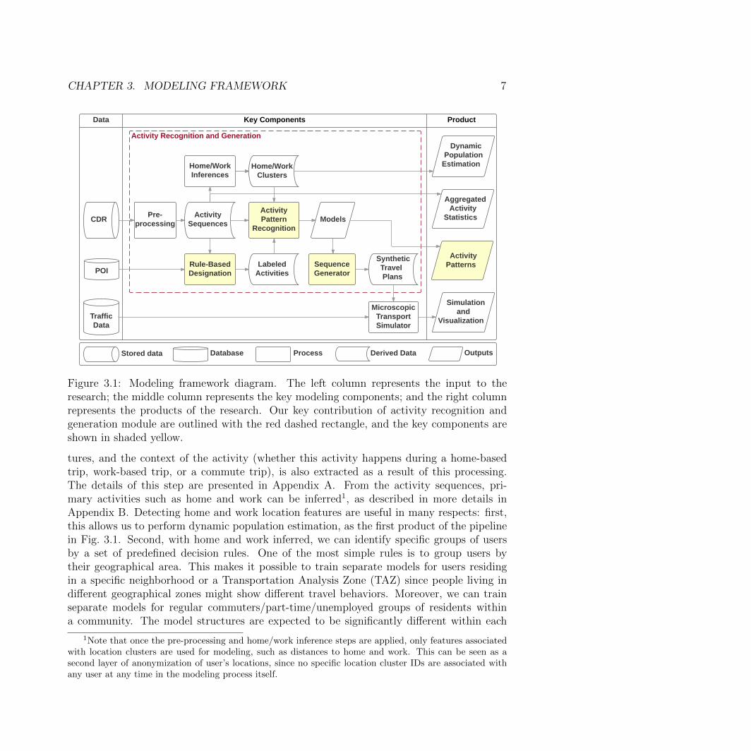
The developed data processing and modeling pipeline is presented in Fig. 3.1. The leftcolumn shows the primary data sources. This includes the cellular call detail data (CDR), acomprehensive point of interest (POI) database within the region of interest, and the trafficdata (vehicle counts, volumes) to calibrate and validate the microscopic traffic simulation.POI databases are usually available from open source maps such as OpenStreetMap, orcomercial APIs such as Google Places API and Factual Places API. These POI databasesprovide a list of POIs and their category labels around a location upon query. These POIinformation is useful in constructing the labeled activities as “ground truth”. The middlecolumn contains the key modules to perform inference and the right column shows theresulting products. Our key contribution is the Activity Recognition and Generation moduleoutlined with the red dashed rectangle, and in particular the components shown in shadedyellow.

Raw CDR data contains a timestamped record for each communication of anonymoususer’s devices served by the cellular network. Due to positioning errors and connection os-cillations, it is not straightforward to extract features to perform activity recognition fromraw CDR sequences. A pre-processing step is first performed to convert the records to asequence of stay location clusters that may correspond to distinct yet unlabeled activities,as shown in Fig. 3.2. The clustering can be seen as a first layer of hashing locations, whichpreserves privacy. Attributes of each activity, such as the start time, duration, location fea-

CHAPTER 3. MODELING FRAMEWORK 7

Activity Recognition and Generation

Data Key Components Product

Pre-processing

CDR

POI

Activity Sequences

Home/WorkClusters

Home/WorkInferences

Rule-BasedDesignation

Labeled Activities

Activity Pattern

Recognition

SequenceGenerator

SyntheticTravelPlans

TrafficData

MicroscopicTransportSimulator

Simulation and

Visualization

Aggregated Activity

Statistics

Dynamic Population

Estimation

Activity Patterns

Models

Stored data Database Process Derived Data Outputs

Figure 3.1: Modeling framework diagram. The left column represents the input to theresearch; the middle column represents the key modeling components; and the right columnrepresents the products of the research. Our key contribution of activity recognition andgeneration module are outlined with the red dashed rectangle, and the key components areshown in shaded yellow.

tures, and the context of the activity (whether this activity happens during a home-basedtrip, work-based trip, or a commute trip), is also extracted as a result of this processing.The details of this step are presented in Appendix A. From the activity sequences, pri-mary activities such as home and work can be inferred1, as described in more details inAppendix B. Detecting home and work location features are useful in many respects: first,this allows us to perform dynamic population estimation, as the first product of the pipelinein Fig. 3.1. Second, with home and work inferred, we can identify specific groups of usersby a set of predefined decision rules. One of the most simple rules is to group users bytheir geographical area. This makes it possible to train separate models for users residingin a specific neighborhood or a Transportation Analysis Zone (TAZ) since people living indifferent geographical zones might show different travel behaviors. Moreover, we can trainseparate models for regular commuters/part-time/unemployed groups of residents withina community. The model structures are expected to be significantly different within each

1Note that once the pre-processing and home/work inference steps are applied, only features associatedwith location clusters are used for modeling, such as distances to home and work. This can be seen as asecond layer of anonymization of user’s locations, since no specific location cluster IDs are associated withany user at any time in the modeling process itself.

CHAPTER 3. MODELING FRAMEWORK 8

Figure 3.2: Call Detail Records (CDR) data processing. The table at left represents theraw CDR format, i.e., time stamped record of communications. A stay points detectionalgorithm (detailed in Appendix A) is used to convert the raw CDR data to a sequence ofstay locations with start time, duration and location ID, as represented in the table at right.

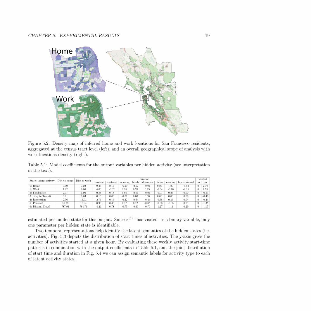
group. Finally, home and work inference for anonymized cellular users adjusted to the fullpopulation provides daytime/nighttime population density estimates, as shown in Fig. 5.2.

With the activity sequences (including home and work anchor activities) identified, wecan understand the daily activity structure of travelers that are traditionally available solelyvia manual surveying. They include: (1) the distribution of number of tours before going towork, during work and after getting back home; (2) the distribution of number of stops duringeach type of tour (home-based, work-based and commute tours); and (3) the interactions instop-making across different times of day (e.g. how making an evening commute stop willaffect the decision in making a post-home stop) [6]. This is the second product of this researchas listed in Fig. 3.1. With the processed activity sequences and inferred primary activities, wecan perform the secondary activity recognition and analyze the activity patterns, includingspatial-temporal profiles of activities and activity transition probabilities. The resultingmodels and analysis will be the third product of the research. To validate the recognitionresults, we collected a small set of ground truth activities based on short range antennaswhich have relatively high spatial resolution. Point of interests (POI) data are joined withthese short range antennas to identify the possible activities performed there and a set ofrules are used to help us collect labeled activities, as detailed in Section 4.3. With the modelcoefficients and a set of sampled home and work locations of the total population, we cangenerate activity sequences and produce synthetic travel plans required by a microscopictraffic simulator. Ground truth traffic counts data are used to validate the simulation resultsand showcase the validity of the presented work for transportation planning and operationspractice. This is the fourth product in Fig. 3.1.

9

Chapter 4

Activity Recognition and Generation

This section introduces main modeling components shown within the red dashed box inFig. 3.1, including activity pattern recognition with IO-HMM, a method of collecting groundtruth activities from short range distributed antenna systems, and a method of simulatingactivity chains from the resulting models.

4.1 IO-HMM for Activity Pattern Recognition

Given the user stay history, that is, a list of stay location features with start times and dura-tions, we would like to convert it into a sequence of activities enriched with semantic labels(“shopping”, “leisure”, etc.), and a heterogeneous context-dependent probability model oftransitions between the activities.

IO-HMM Architecture

Hidden Markov Models (HMMs) have been extensively used in the context of action recog-nition and signal processing. However, standard HMMs assume homogeneous transition andemission probabilities. This assumption is overly restrictive. For instance, if a user engagesin a home activity on a weekday, and departs for the next activity in the morning, she islikely going to work. If she departs in the evening, the trip purpose is likely to be recreationor shopping. Therefore, we propose to use the IO-HMM architecture that incorporates con-textual information to overcome the drawbacks of the standard HMM. In Fig. 4.1, the solid(blue) nodes represent observed information, while the transparent (white) nodes representlatent random variables. The top layer contains the observed contextual variables ut, suchas time of day, day of the week, and information about activities in the past (such as thenumber of hours worked on that day). Note that the values of the input variables ut usedto represent the context have to be known prior to a transition. The middle layer containslatent categorical variables zt corresponding to unobserved activity types. The bottom layer

CHAPTER 4. ACTIVITY RECOGNITION AND GENERATION 10

zt-1

ut-1

xt-1

zt+1

ut+1

xt+1

zt

ut

xt

zt-1

ut-1

xt-1

zt-1

ut-1

xt-1

Figure 4.1: IO-HMM Architecture. The solid nodes represent observed information, whilethe transparent (white) nodes represent latent random variables. The top layer contains theobserved input variables ut; the middle layer contains latent categorical variables zt; and thebottom layer contains observed output variables xt.

contains observed variables xt that are available during training of the models (but not whengenerating activity sequences), such as location features and duration of the stay.

Likelihood of a data sequence under this model is given by:

L (θ,x,u) =∑z

(Pr (z1 | u1;θin) ·

T∏t=2

Pr (zt | zt−1,ut;θtr) ·

T∏t=1

Pr (xt | zt,ut;θem)). (4.1)

IO-HMM architecture has been well described in [5]. Variable notation and importantdifferences between IO-HMM and standard HMM are summarized in Table 4.1.

Parameter Estimation

IO-HMM includes three groups of unknown parameters: initial probability parameters (θin),transition model parameters (θtr), and emission model parameters (θem). Expectation-Maximization (EM) is a widely used approach to estimate the parameters of IO-HMM. TheEM algorithm consists of two steps.

E step: Compute the expected value of the complete data-log likelihood, given theobserved data and parameters estimated at the previous step.


Table 4.1: Highlights of comparison between an HMM versus. IO-HMM (ut, zt, xt denoteinput, hidden and output variables respectively, i is an index of a hidden state, t is a sequencetimestamp index).

HMM IO-HMMinitial state probability πi Pr (z1 = i) Pr (z1 = i | u1)transition probability ϕij,t Pr (zt = j | zt−1 = i) Pr (zt = j | zt−1 = i,ut)emission probability δi,t Pr (xt | zt = i) Pr (xt | zt = i,ut)forward variable αi,t δi,t

∑l ϕli,tαl,t−1, with αi,1 = πiδi,1

backward variable βi,t∑

l ϕil,tβl,t+1δl,t+1, with βi,T = 1complete data likelihood Lc

∑i αi,T

posterior transition probability ξij,t ϕij,tαi,t1βj,tδj,t / Lc

posterior state probability γi,t αi,tβi,t / Lc

M step: Update the parameters to maximize the expected data likelihood given by:

Q(θ,θk

)=∑i=1

γi,1 log Pr (z1 = i | u1;θin)

+T∑t=2

∑i

∑j

ξij,t log Pr (zt = j | zt−1 = i,ut;θtr)

+T∑t=1

∑i

γi,t log Pr (xt | zt = i,ut;θem) . (4.2)

In the above, Q(θ,θk

)is the expected value of the complete data log likelihood; k

represents the EM iteration; T is the total number of timestamps in each sequence; ut,zt and xt are the inputs, hidden states, and observations at step t; and θ are the modelparameters to be estimated. The meaning of other variables is given in the first column ofTable 4.1.

Transition and Emission models

The parameter estimation procedure of IO-HMM described above implies that any supervisedlearning model that supports gradient ascent on the log probability can be integrated into theIO-HMM. For example, in Equation 4.2, each of the model parameters (θ) can be estimatedwith neural networks. A neural network with a softmax layer can be used to learn theinitial probability parameters (θin) through back-propagation, another neural network witha softmax layer for learning the transition probability parameters (θtr), and a third withcustomized layers for estimating emission model parameters (θem).

Note that the EM algorithm can be naturally implemented in a MapReduce framework,a programming model and an associated implementation for processing large data sets on


computing clusters. The Expectation step can be fit into the Map step, calculating theposterior state probability γ and posterior transition probability ξ in parallel for each trainingsequence. The estimated posterior probabilities γ and ξ are collected in the Reduce step.The source code of an implementation developed as a part of this research is available fromhttps://github.com/Mogeng/IO-HMM.

4.2 Model Specification

Input-Output Variables

In practice, models of simple structure (linear, multinomial logistic, Gaussian) with inter-pretable variables and parameters are preferred. For example, in an application below, weinclude the following input variables ut: (1) a binary variable indicating whether the dayis a weekend; (2) five binary variables indicating the time of day that the activity starts,morning (5 to 10am), lunch (10am to 2pm), afternoon (12 to 2pm), dinner (4 to 8pm) ornight (5pm to midnight); and (3) for the users with identified work location, the number ofhours the user has spent at work this day. This variable contains accumulated knowledge onthe past activities.

The IO-HMM model also includes the following outputs xt at each timestamp t: (1) x(1),the distance between the current stay location and the user’s home; (2) x(2), the distancebetween the current stay location and the user’s work place; (3) x(3), the duration of theactivity; and (4) x(4), whether the user has visited this stay location cluster previously.

The selection of the inputs and outputs is guided by common knowledge. The activitystart time is relevant for differentiating activity types. The number of hours worked in a dayis a strong indicator of a person’s likelihood to return to work (after a midday activity, forexample). The model inputs contain information that is known at the start of the transitionto a new activity. In contrast, the output features contain information that is not availableat the transition to a new activity. For example the duration and the location or land-use inthe vicinity of a new activity is unknown at the time of the transition. In other words, outputvariables can be observed when training the models, but must be inferred when samplingsequences of activities from the model.

The model outputs have a strong dependence on the activity type. For example, thedistance that a person is willing to travel from home for a leisure trip may be longer thanthe distance that a person is willing to travel for a shopping trip. The duration dependsboth on the activity type, activity start time, and on the previous activities in the day. e.g.,the expected duration of a work activity will decrease if a person has already worked in theday.


Initial, Transition and Emission Models

Multinomial logistic regression models are used as the initial probability model and transitionprobability models. Note that for succinctness, we use θ in each of the following equationsto represent the θin,tr,em in Equation 4.2. The first term of Equation 4.2 can be written as:

Pr (z1 = i | u1;θ) =eθiut∑

k eθkut

. (4.3)

The θ for initial probability model is a matrix with the ith row (θi) being the coefficientsfor the initial state being in state i. The second term of Equation 4.2 can be written as:

Pr (zt = j | zt−1 = i, ;θ) =eθjiut∑

k eθki ut

. (4.4)

The θ for transition probability models is a set of matrices with the jth row of the ith

matrix (θji ) being the coefficients for the next state being in state j given the current statebeing in state i.

To gain interpretability, we use linear models for the outputs represented as continuousrandom variables. We assume a Gaussian distribution for the distance to home and workvariables x(1) and x(2) and the activity duration variable x(3). Where x(1) and x(2) dependonly on the hidden activity type, the duration variable x(3) depends on the hidden activityand also the contextual input variables. The third term of Equation 4.2 can be written as:

Pr (xt | zt = i,ut;θi) =1√

2πσie− (xt−θi·ut)

2

2σ2i , (4.5)

The θ for one such output emission model is a set of arrays where θi and σi denote thecoefficients and the standard deviation of the linear model when the hidden state is i. Whilewe chose to represent outputs x(1),(2),(3) as Gaussian random variables, Gamma regressioncould be applied to duration x(3) to capture the non-negative, continuous, and right-skewednature of these response variables. Moreover, response variables x(1) and x(2) could be mod-eled simultaneously using multivariate linear regression to capture the correlations betweendistance to home and distance to work.

Output x(4) is a binary variable, and we used logistic regression model as the outputmodel. The probability in the third term of Equation 4.2 can be written as:

Pr (xt = 1 | zt = i,ut;θi) =1

1 + e−θi·ut. (4.6)

Finally, we emphasize that an activity label is just a latent categorical variable. A seman-tic label can be associated to it following an in-depth analysis the we present in Section 5.2below.


4.3 Model Selection

Model selection for IO-HMM includes the choice of the number of hidden states. One wouldlike to set a high number that encompasses a wide variety of travel purposes, however, dataquality and availability limits the number of feasibly identifiable activities. Moreover, anambiguity in semantic meaning of activity types (consider “leisure” versus “recreation”)asks for limiting the number of hidden states that show useful in practical applications. Wedescribe here an empirical procedure for collecting ground truth data on activity types thatprovide useful insights on these modeling choices. The number of hidden states of the IO-HMM model are set according to the labels of these ground truth activities. For CDR, itis usually hard to collect ground truth activities due to its low spatial resolution. However,there is a set of short range antennas that serve only a small range of area, which haverelatively high spatial resolution. These short range antennas provide us the opportunity tocollect “ground truth” activities.

Short Range Distributed Antenna Systems (DASs)

A common component of a cellular networks is a set of distributed antenna systems (DASs)that are short ranged, including Indoor DASs (IDASs) and Outdoor DASs (ODASs). IDASsare usually installed in large commercial buildings such as shopping malls to ensure bettersignal coverage. And ODASs are usually installed at high occupancy outdoor venues suchas stadiums or concert arenas. These antennas are set up to maximize signal strength forthe users located in the building or stadium served by a given DAS, ensuring more preciselocalization. Fig. 4.2 illustrates the times and durations of connections established by usersserved by three particular DASs. The patterns are structured in time, indicating the activitiesperformed there are quite regular and their purpose can be inferred from domain knowledgewith high confidence.

Designation of Rules for Ground Truth

IDASs are often installed in large mixed-use commercial buildings. For example, one com-mercial building with IDAS installed could have bakeries, restaurants, taxi stands, gym andfitness centers, retail stores, as well as other businesses such as accounting and financialservices. We designed a set of spatial-temporal decision rules to label a set of activities thatcan be considered as the ground truth. For instance, if a user is connected to a DAS ina food court at noon for one hour, this is most likely to be indicative of a lunch activity.Although we do not have complete certainty that this is indeed the activity type, the eventis indistinguishable from a lunch break in terms of its mobility footprint, and with highlikelihood we interpret this as a food activity.

We first acquired place information from POI databases such as Google places API andFactual Global Places API. Then, we joined this information with the locations of the DASsin order to extract activities that could be performed at each DAS. The place information


(a) DAS in a major train station used by suburban commuters.

(b) DAS in a fitness center with multiple recreational health studios.

(c) DAS in a business district building with a large food court.

Figure 4.2: Structural patterns of empirical data collected at short range DASs well explainthe activity performed around the DASs: the number of activities start times within a courseof a week (left) and an empirical joint distribution plot of the visit duration versus start times(right).


Table 4.2: Rules of labeling secondary activities based on activity spatial-temporal features

ActivityDuration(hours)

Starthour

ContextLocationcategory

Lunch 0.25 - 1 11-12 FoodDinner 0.25 - 2 17-18 Food

Shop 0.25 - 17-914-1520-21

Home based or duringevening commute

Shop

Transport < 0.25 Commute Transport

Recreation 1-4 7-21Home based or duringevening commute

Recreation

Personal any 7-21 PersonalTravel any any Out of the region

provides listings of local business and point of interest (POI) at most given locations. Sincemultiple activities can happen at the same location, we need some additional rules based onthe spatial-temporal features of activities, as shown in Table 4.2. The “location category”column of the table indicates that the category is among the category labels returned fromthe APIs.

Note that the rules used to label activities as reported in Table 4.2 are restrictive. Giventhat the main purpose of these labels is to validate the proposed models, our goal is tobe very confident in the activities we label. Thus, these rules are designed to pursue highprecision rather than high coverage.

4.4 Activity Chains Generation

One of the strengths of the proposed generative state-space model is that it can generatesequences of activities based on the parameters θ estimated for each user or shared acrossa group of users believed to have similar mobility lifestyle. For example, a working dayscenario can be generated as follows. A synthetic population with a predetermined homeand work locations is created according to the population census. Each user is assumedto begin her day at home, z1 = 0. Relevant context information ut and learned transitionPr (zt = j | zt−1 = i,ut) and emission probabilities (4.5)-(4.6) are then used to determinethe next state and sample output variables for the activity duration and location fromthe posterior. At the end of this activity the relevant context information ut is updatedand the next activity is selected given the newly obtained transition probabilities. Theprocess continues until the full daily sequence of activities has been generated. We discussthe interpretation of the posterior probability distributions and report on an experimentalvalidation of this approach below.

17

Chapter 5

Experimental Results

This section describes a full-scale regional experiment where we train IO-HMM for commutersfrom each of the 34 super-districts in the San Francisco Bay Area, in order to develop anactionable mobility model for a typical weekday. First we show how one can interpretthe model parameters and evaluate activity recognition capability, using the City of SanFrancisco (SF) as an example. Next, we use the trained models for all 34 super-districtsto generate sequences of activities for a regional agent-based traffic micro-simulation, andcompare the results with the observed traffic volumes.

The data used in these studies comprise a month of anonymized and aggregated CDR logscollected in Summer 2015 by a major mobile carrier in the US, serving millions of customersin the San Francisco Bay Area. No personally identifiable information (PII) was gathered orused for this study. As described previously, CDR raw locations are converted into highlyaggregated location features before any actual modeling takes places.

5.1 Data Pre-processing

We pre-process the data following the steps in Appendix A. The home and work locationsare identified during the pre-processing step. We take cell phone users that:

• showed up for more than 21 days a month at their identified “home” place;

• showed up for more than 14 days a month at their identified “work” place;

• have home and work not at the same location.

These criteria identify regular working commuters with a day structure containing bothdistinct Home and Work. Empirical distributions of the average number of daily activities forthis population is shown in Fig. 5.1. The median number of activities is 4.4 per weekday and4.0 per weekend. This is consistent with the California Household Travel Survey, reportinga number of 4 activities per day [1].

Fig. 5.2 shows the density map of inferred home and work locations for San Franciscoresidents, aggregated at the census tract level. As shown in the right of Fig. 5.2, the work

CHAPTER 5. EXPERIMENTAL RESULTS 18

(a) Weekday (b) Weekend

Figure 5.1: Empirical distributions of the average number of daily activities of San Franciscosubscribers on a weekday (left) and on a weekend (right), after pre-processing.

locations are spread in the SF Bay Area. The highest density occurs in San Francisco,Oakland, and some South Bay cities. Focusing on work locations in San Francisco, manyof the inferred work locations are in Downtown San Francisco, the Financial District, andSoMA - three San Francisco neighborhoods with high employment density [21]. As expected,the home locations are more spread out throughout the city.

While individual users with long sequences of observations can be modeled with fullypersonalized IO-HMM, such processing violates privacy protection regulations of the carrier.An application of the IO-HMM presented below is trained with parameters shared across agroup of users with similar geographical and structural properties of the day. It not only pro-vides computational advantages, but also simplifies scenario evaluation for the practitionerswho operate with socio-demographic groups rather than individuals. In this paper, we sim-plified the grouping method to be based on geographical boundaries, such as super-districtsdefined by the San Francisco Metropolitan Transportation Commission (MTC).

5.2 Activity Recognition Results

In this section we interpret the results of the IO-HMM that has been fit to the four super-districts that make up the city of San Francisco. The model was trained on a group of20,000 anonymous San Francisco residents (about 2% of the population). The coefficientsof trained emission models are reported in Table 5.1. Recall that we use linear models asthe output models for x(1), distance to home, x(2), distance to work, and x(3), duration ofthe activities. Logistic regression was used as the output model for x(4), cluster has beenvisited before. Since x(1) and x(2) depend only on the hidden activity, only the intercepts areestimated. For x(3), we specify that the duration depends on activity type and also on the“day of week”, “time of day” and “hours worked” input variables, there are 8 coefficients


Figure 5.2: Density map of inferred home and work locations for San Francisco residents,aggregated at the census tract level (left), and an overall geographical scope of analysis withwork locations density (right).

Table 5.1: Model coefficients for the output variables per hidden activity (see interpretationin the text).

State: latent activity Dist to home Dist to workDuration Visited

constant weekend morning lunch afternoon dinner evening hours worked no yes0: Home 0.00 7.22 9.45 2.17 -6.29 -2.57 -0.94 0.20 1.29 -0.03 0 2.191: Work 7.22 0.00 4.00 -0.02 2.98 0.76 0.19 -0.64 -0.10 -0.26 0 1.762: Food/Shop 2.37 1.90 0.84 0.18 0.00 -0.01 -0.04 -0.01 0.25 0.00 0 -0.533: Stop in Transit 3.21 3.63 0.16 0.00 -0.01 0.00 0.00 0.00 0.00 0.00 0 -0.464: Recreation 2.36 15.03 2.76 0.17 -0.42 -0.64 -0.45 -0.68 0.37 0.04 0 -0.445: Personal 18.79 16.94 0.93 0.46 0.17 0.12 -0.05 -0.03 -0.05 0.01 0 -1.356: Distant Travel 787.94 784.71 4.26 0.78 -0.75 -0.39 -0.76 -1.27 1.11 0.29 0 -1.17

estimated per hidden state for this output. Since x(4) “has visited” is a binary variable, onlyone parameter per hidden state is identifiable.

Two temporal representations help identify the latent semantics of the hidden states (i.e.activities). Fig. 5.3 depicts the distribution of start times of activities. The y-axis gives thenumber of activities started at a given hour. By evaluating these weekly activity start-timepatterns in combination with the output coefficients in Table 5.1, and the joint distributionof start time and duration in Fig. 5.4 we can assign semantic labels for activity type to eachof latent activity states.


Figure 5.3: Number of activities (labeled per highest posterior probability) by their respectivestart time within a course of a week.

Primary Activities: Home and Work

Latent activity state 0, shown in green in Fig. 5.3 is easily identifiable - it is the “home”activity. The typical start time ranges from 3pm to midnight. The home activity exhibitsgreater variation in start time on Friday and weekends than on other weekdays. The positive“weekend” coefficient on the duration of this activity indicates that people stay at homelonger during weekends.

The temporal profile of home activities in Fig. 5.4a has two major clusters. The uppercluster indicates regular overnight home activities. This cluster can be further separated intotwo clusters. One peaks at 6pm, representing the home activity directly after work. Theother peaks at 9pm, representing the home activity after some secondary activities in theevening. Since the home activity duration is generally set by the regular work start hour,the downward slope of the upper cluster signifies that if a user arrives at home later in theday, they are likely to spend fewer hours at home.

Activity state 1, shown in blue in Fig. 5.3 is the “work” activity. It has highest peaks inFig. 5.3, signifying that it is a very regular activity with concentrated start times.

According to Table 5.1, a work activity has a base duration of 4 hours, if it starts in themorning, the user is likely to stay 2.98 hours longer, that is 6.98 hours in total; if it beginsin the afternoon or evening the average duration is shorter. As a compounding effect ofreturning to work in the afternoon or evening, the “hours worked” column indicates that theexpected duration will decrease by 0.26 hours for every hour that the user already spent atwork in the day. The “is weekend” column indicates that if a user chose to work on weekend,the average work activity duration is not significantly different from that on weekdays; notethat (from Fig. 5.3) the probability of visiting the work activity is much lower on the weekend.The “visited” column indicates the propensity of the location being frequently revisited. Forthe work activity, the coefficient 1.76 indicates a very high likelihood of returning to thesame location to perform the same activity.

From Fig. 5.4b, we can see that the temporal profile of work activities has three clusters.The upper cluster indicates regular “9 to 5” work activities without a break. The lowerleft cluster represents the morning work activities and the lower right cluster represents theafternoon work activities. All three clusters are tilted at -45 degrees. This is due to theusually fixed lunch hour at noon and end of work at about 5pm.


Secondary Activities

The remaining states are secondary activities. Activity 2 peaks in start time around noonand in the evening. As shown in Table 5.1, activity state 2 has an average duration of about0.84 hours, and is close to both home and work place. As shown in Fig. 5.4c, the duration ofthis activity is slightly longer in the evening. Based on these properties, we assign activity 2the label “food/shop”. From Fig. 5.3 we see that, on weekends, this activity peaks at noon.The weekend activity duration, according to Table 5.1, is about 0.2 hours longer than it ison weekdays.

Activity 3 is located close to home and work, and has an average duration of about 10minutes, according to Table 5.1. From Fig. 5.4e, we can see that this activity peaks inthe early morning and late afternoon right before home activity. Fig. 5.4d and Table 5.1also indicate that the duration is not affected by time of day or day type (weekend versusweekday). From Fig. 5.3, we can see that this activity is visited more frequently on weekdaysthan weekends, indicating that the activity could be an in-commute activity such as coffee,transport, or picking up kids. It is worth noting that although activity 3 is less revisitedthan home and work activities, it is more likely to be revisited compared to other activities.This gives us more confidence in labeling them as regular activities such as “Short Stop inTransit”.

We have assigned activity state 4 a label of “recreation”. As seen in Table 5.1, the activityis quite close to home but far from the work place. The state has an average duration of 2.7hours, much longer than the durations of activity state 2 and 3. This activity last longerin evening hours or weekends. As shown in Fig. 5.3, this activity often starts in the earlymorning or evening hours on weekdays, and tellingly, more users engage in this activity onFridays and weekends.

We have assigned activity state 5 a label of “personal”. The distances from home andwork are 19 and 17 miles, respectively, and the average duration of this activity is 0.93 hours.This state could encompass both off-site work related trips and/or longer-distance dining orleisure activities. As shown in Fig. 5.3. Due to the distance of this activity, more usersengage in this activity on weekends and this activity is least likely to be revisited.

Activity state 6, labeled “distant travel”, or more accurately activities that occur whiletraveling, is the most irregular and infrequent. The average distances from home and workare quite high (average 800 miles). This activity type seems to occur predominantly onFridays and weekends according to Fig. 5.3.

Activity Transitions

We omitted “distant travel” activity from the transition matrix since if a person is travelinga long distance, the next activity is also most likely to be categorized as “distant travel”;the distance dominates the state. Fig. 5.5a shows the transition matrix associated withmornings. The labels on the left indicate the state the user is transitioning from, andthe labels on the top indicate the state the user is transitioning to. The most significant


(a) 0: Home (b) 1: Work (c) 2: Food/Shop

(d) 3: Stop in Transit (e) 4: Recreation (f) 5: Personal

Figure 5.4: Joint distribution plot of duration and start hour per activity type. The labelsare gained by assigning the activity to the one with the highest posterior probability aftertraining.

transition is from “home” to “work.” Fig. 5.5b shows the transition matrix associated withevenings. The transitions from all other states to “home” are significant. However, if theuser’s transition from activity is “home”, then she is more likely to transition to “food” or“recreation” activities. Fig. 5.5c shows the transition matrix in the afternoon, for users whohave not yet visited the “work” state in the day. For these users, there is a high probabilityof going to work. As in Fig. 5.5d, by keeping all the input context information equal as inthe previous case, and only specifying that the simulated user has previously worked for 5hours on that day, one can see that the probability of going to work is significantly reduced.


(a) Morning (6-10am) (b) Night (5pm-midnight)

(c) Afternoon (12-2pm), users who have not vis-ited work

(d) Afternoon (12-2pm), users who have worked5 hours

Figure 5.5: Heterogeneous activity transition matrices under different contextual variables.

5.3 Evaluation of Activity Recognition

Recognition Accuracy

The distribution of collected ground truth activities are biased and do not correspond to thetrue distribution of urban activities. To reasonably evaluate performance of IO-HMM, we


Table 5.2: Confusion matrix of inferred activities versus “ground truth” activities

Ground TruthAnnotations

Home Work Food/Shop Transit Recreation Personal TravelHome 9994 0 0 0 1 1 4 0.999

Recall

Work 0 7495 0 0 0 2 3 0.999Food/Shop 0 0 3013 413 1307 267 0 0.603

Transit 0 0 31 6980 359 130 0 0.931Recreation 0 0 1519 0 1403 78 0 0.468Personal 0 0 321 17 84 3426 152 0.857Travel 0 0 0 0 0 11 989 0.989

1.000 1.000 0.617 0.942 0.445 0.875 0.8620.876

Precision

Table 5.3: Comparison of model accuracy

ModelAll Activities Secondary Activities

Accuracy F1 Accuracy F1HMM 0.859 0.783 0.739 0.698

Partial IO-HMM 0.866 0.824 0.752 0.754Full IO-HMM 0.876 0.827 0.771 0.758

need to sample a subset of ground truth activities so that the sample weight is consistentwith the true distribution of urban activities. According to the the distribution given by the2015 Travel Decisions Surveys (TDS), conducted by San Francisco Municipal TransportationAgency (SFMTA)[31], we sampled (scaled) 10000 home activities, 7500 work activities, 5000Food/Shop activities, 7500 Stop in Transit activities, 3000 recreation activities, 4000 personalactivities and 1000 Travel activities.

Overall, we get 87.6% accuracy on all activities, with a macro-precision of 82%, a macro-recall of 83.5% and a macro-f1 score of 0.827. Here we reiterate that there are no explicitground truth labels on traveler’s activities; instead the ground truth labels refer to theidentifiable activities that occur near short-range antennas (labeled according to Table 4.2)and activities that occur at the inferred home or work location.

From the confusion matrix in Table 5.2, we can see that most confusion happens be-tween “food/shop” and “recreation” activities. This is natural because “food/shop” and“recreation” activities are similar in time and space. We also notice that some “food/shop”activities are mistaken as a “short stop in transit”, this is because some “food/shop” activi-ties and “stop in transit” are close in space, thus some short “food/shop” activities are takenas “stop in transit” because of the duration. Since the activities that we labeled as “per-sonal” are mainly medium distance activities that could encompass longer-distance dining,some “food/shop” activities could also be confused as “personal”.

To compare the performance of different models, we also report the accuracy of (1)Hidden Markov Models (HMM) with the same output as IO-HMM but with no inputs; (2)


Partial IO-HMM with transition probabilities dependent on inputs while all emissions areonly conditioned on hidden states; and (3) Full IO-HMM as described, in Table 5.3.

We report the accuracy and macro-f1 score as metrics of success for our models. F1 scorecan be interpreted as a weighted average of the precision and recall. For multi-class tasks,macro-f1 score calculates the average per-class precision and recall and then perform the f1score calculation. We can see that the full IO-HMM has the best performance. Since “home”and “work” are rather easy to infer, we also report the performance for secondary activitiesonly. For the five class classification task, we get 77.1% accuracy. Another observationis that the macro-f1 score of the partial and full IO-HMMs do not differ too much, butall outperform the pure HMM. These results exhibit the benefits of the context-dependenttransition models.

We see that the full IO-HMM outperforms the partial IO-HMM slightly which outper-forms the pure HMM. Since “home” and “work” have high accuracy, the improved perfor-mance is mainly in secondary activity recognition. In all cases, f1 score is smaller than theaccuracy. This is because the class that has higher support also has higher accuracy. Sinceaccuracy score is a weighted average with support while macro-f1 score is an unweightedaverage, f1 score is lower than the accuracy.

Survey-derived statistics

Another way to evaluate the method is to compare our model with aggregated statisticsfrom surveys. We consider the Travel Decisions Survey (TDS), which contains 1000 randomdigit dial and cell phone samplings in the area of interest. Overall, the activity proportionsof our model match with TDS. If we split our Food/Shop activities into half food and halfshop, food and recreation is 20% in our model versus 21% in TDS; shopping and errand(personal) is 21% in our model versus 20% in TDS. Work/school activity is 22.5% in ourmodel versus 23% in TDS. The main difference is with the “Home” activity, for which TDSreport a proportion of 35%, which is a little higher than the proportion of 30% reported byour model. This discrepancy is likely due to under-reporting of secondary activities in TDS.

5.4 Activity Generation from an IO-HMM

One of our goals is to enable activity based travel demand models that use cellular datato create synthetic agent travel patterns without compromising the privacy of cell phoneusers. As such, we test our models’ generative power in the Bay Area context — we simulate463, 000 agents in the Bay Area (15% sample of the commuters) and create a day-long activityplan for all agents with anticipated start-times, locations, and durations of all activities inthe day.

As travel patterns vary greatly over the region, we trained 34 IO-HMMs, each for asubset of cell phone users residing within each of the 34 super-districts as defined by the SanFrancisco Metropolitan Transportation Commission (MTC). Using the Iterative Proportional


Fitting [14] procedure to fit the population marginals with the census data, we sampleresidents home and work locations to create synthetic driver with a predetermined homeTAZ and work TAZ. The numbers were further adjusted according to occupancy statisticsfrom CHTS (single driver, two and multi-person carpool). The precise home and worklocations (lat/lon coordinates) are sampled uniformly within the home and work TAZs.

Each simulated user is assumed to start her day at home. The home departure time andthe transition time are drawn from their respective distributions to determine the start timeof the first activity. Home departure times for the first non-home activity of the day aremodeled as Gaussian random variables with super-district dependent mean departure timeand standard deviation calibrated from CDR records. As IO-HMM is trained on the observedtravel sequences with revealed departures times, we assume that it captures the dependenciesof transition times on the origin and destination, travel mode and traffic conditions.

Generation continues until the activity start time reaches midnight. At every step, previ-ous activity state and context information are used to obtain transition probabilities from theIO-HMM and sample the next activity state according to the transition probabilities. Afterthe activity type has been selected, the activity duration is sampled from a truncated normaldistribution with mean and standard deviation coming from output x(3) of the IO-HMM.Next, the activity location is selected - if the activity is a home-activity or work-activity, theexercise is trivial. If not, we use IO-HMM outputs x(1) and x(2) - the distance between thestay location and the user’s home output and distance from the stay location to the user’swork output from the IO-HMM to generate a new destination TAZ from the choice set ofTAZs within matching distances. The precise location of the activity is sampled uniformlyfrom the selected TAZ. Note that future research on destination location choice models couldimprove the location selection process for secondary activities.

Due to the nature of IO-HMM, we must filter out and discard unrealistic activity chainsgenerated in this process. We determine unrealistic activity chains to be chains that donot end the day at home and activity chains where 3 or more of the same activity typeoccur in a row. These filters constrain the overall structure of the day to be aligned witha feasible/conventional day structure. For simulation purposes we also filter activity chainsthat include long-distance travel out of the Bay Area. Fig. 5.6 presents 4 common andinteresting (among top 20) activity patterns generated from IO-HMM model.

Overall, the aggregated statistics of activity patterns match with the travel surveys. Forexample, the percentage of US employed person who go to work on an average weekday is82.9% [25], this number is 83.7% for our simulated population. Considering the summarystatistics for people who go to work, we compare the percentage of people who participatein activities at different times of day. The percentage of people participating in at least oneactivity before morning commute, during morning commute and after work is 3.1%, 14.8%and 46.3% in the Bay Area Travel Survey [6] and these numbers are 2.9%, 15.2% and 43.7%in our simulated population.


Figure 5.6: Distribution of activity start times over a course of a day of four example commonactivity patterns generated from the Bay Area IO-HMMs. Note that all simulated activititypatterns start at home, so (a) designates the Home-Work-Home travel pattern. The x-axisdesignates the start time of the activity, the y-axis represents the proportion of trips (forusers with this activity pattern) starting at this time.

5.5 Evaluation via Traffic Micro-simulation

Traffic micro-simulation is a conventional approach in studying performance and evaluatingtransportation planning and development scenarios. Ground truth observations of the flowsat sections of the road network provide an independent data source that can be used toevaluate the accuracy of the activity generation model. We present here a summary of thevalidation results based on the traffic volume data collected by the California DOT freewayPerformance Management System (PeMS) in the 9 counties of the Bay Area (see Fig. 5.7).Micro-simulation of a typical weekday traffic is performed using the MATSim platform [2].MATSim is a state-of-the-art agent based traffic micro-simulation tool that performs trafficassignment for the set of agents with pre-defined activity plans. It varies departure timesand routing of each agent depending on the congestion generated on the network, in order tomaximize agent’s daily utility score. We have compared the results of the flows produced onthe Bay Area network containing all freeways and primary and secondary roads (a total of24’654 links) from the generated activity sequences with the observed traffic volumes. As themodel is trained to reproduce average weekday, hourly traffic volumes are taken as averagesover all weekdays (except for Mondays and Fridays) of Summer 2015. The simulation is runat 15% of the total population, and the road capacities as well as total resulting counts arescaled accordingly.

Note that observed traffic counts are not used for model calibration. They are used asindependent data to evaluate the validity of the synthetic travel sequences produced withIO-HMM. The locations of the sensors on the road network are presented in Fig. 5.7. Italso demonstrates examples of the three characteristic hourly volume profiles comparingthe modeled and observed counts. The results for the full set of sensors are presented


Figure 5.7: A fragment of the SF Bay Area road network with the location of 600 trafficvolume detectors used for validation (shown with small black dots). Inlet graphs illustratethree sample hourly vehicle volume profiles for observed (orange) and modeled (blue) flowson a typical weekday in Summer 2015.

in Fig. 5.8. Fig. 5.8a shows a comparison of the volumes for three distinct time periods.Fig. 5.8b summarizes the validation results over all 600 sensors in terms of the relative error


(a) Modeled versus observed volumes at 8am(black),1pm (red) and 6pm (blue) (r2 =0.81, p < 10−3).

(b) Mean relative error (%) over all 600 sensors ofmodeled versus observed traffic volumes during theday over all 600 sensors.

Figure 5.8: Micro-simulation validation with the observed freeway traffic volumes

(% volume) over-/under-estimated by the model as compared to the ground truth. Onecan notice lower accuracy at night and early morning hours explained by the fact that themodel was developed and applied on a subset of daily commuters and did not include a largeportion of trips performed by unemployed population and people working from home, besidesmultiple other traffic components (commercial fleets, taxis, visitors) that are out of scope ofthe model. Despite it’s relative simplicity, the model has demonstrated a reasonable accuracy(r2 = 0.81, p < 10−3 in Fig. 5.8a ) as compared to the ground truth data. A thoroughcomparison between the activity chains generated from IO-HMM model and baseline modelssuch as the one developed by regional transportation planning authorities and based onsurveys is ongoing and its preliminary results are available from the author by request.

30

Chapter 6

Conclusion and Future Work

In this paper, we developed a scalable and interpretable model for regional mobility analysisfrom cellular data. As an illustration, we inferred the activity patterns including primary, sec-ondary activities and heterogeneous activity transitions of a set of anonymized San FranciscoBay Area commuters using an unsupervised generative state-space model. We validated thisinference by comparing it with (1) 2015 Travel Decisions Surveys (TDS) on the aggregatedactivity statistics; and (2) a set of ground truth activities based on short range distributedantenna system (DAS); (3) observed volumes of vehicular traffic flow in the regional roadnetwork on an average weekday. To examine the generative power of the model, we synthe-sized travel plans for each agent with home and work locations sampled from census data.An agent-based microscopic traffic simulation was conducted to compare the resulting trafficwith real traffic, and a reasonable fit accuracy was observed. An interesting extension tothis work is to compare the activity sequence generation power of different techniques, frombaseline models with only home and work activities to more advanced IO-HMM models andrecurrent neural network such as long short term memory (LSTM) models.

Several improvements can be built upon the presented work. Partitioning a populationinto sub-groups (whether socially or spatially) for shared parameter modeling is a partly openproblem. Currently we approached it by defining rules to identify groups of a similar daystructure, and applying geographic constraints. This step will be compared to an alternativespecification that involves a mixture of IO-HMM models.

With privacy concerns and data limitations in mind, the location choice model imple-mented in this paper is relatively simple. Future work may incorporate a discrete choicemodel on a set of TAZs so that locations can be directly sampled when generating activitysequences.

Activity patterns inferred and analyzed in this paper reveal the spatial and temporalprofile of activities of regular commuters, as well as the heterogeneous transition probabilitiesdependent on contextual information. The generative nature of our proposed model allowsto sample accurate travel scenario inputs needed by activity based travel micro-simulationmodels. A range of issues remain where the advantages of using cellular data alone arenot straightforward. This includes travel mode detection, identification of the number of

CHAPTER 6. CONCLUSION AND FUTURE WORK 31

car-pools, modeling short-range and non-motorized travel to name a few. Nevertheless, suchmethods derived from automatically and continuously collected cell phone data are bound tomake a substantial impact on urban and transportation planning, and represent a significantimprovement upon the state-of-the-art.

32

Appendix A

Stay points detection in CDR

The goal of stay location recognition is to turn CDR logs into a list of sequential stay locationidentifiers with start time and duration for each user, as illustrated in Fig. 3.2. Each recordof raw CDR logs contains the timestamp and the approximated latitude and longitude ofevents recorded by the data provider. This is a CDR-specific step that requires fine-tuningof several threshold parameters. Note that once the pre-processing steps described in thisAppendix and the following are applied, only features associated with clusters locations areused, such as distances to home and work. This can be seen as a layer of anonymization ofuser’s locations, since no specific location cluster IDs are further associated with any userat any time in the activity modeling process itself. The main steps of the algorithm are asfollows:

(1) Cluster CDR records. The first step in stay location detection is filtering out po-sitioning errors. This is achieved by spatial clustering. For GPS data, accuracy ranges of10-100m are used in many studies that use GPS to detect stay locations [11]. The distancethresholds for GPS stay-location clustering is much smaller than the thresholds for CDRrecords. For example, a roaming distance of 300 meters [20] and 1000 meters [35] was usedto cluster points to reflect the spatial measurement accuracy of the CDRs. For our stay-location detection, we use a density based clustering with similar parameters. At the endof the clustering step, consecutive data points with the same cluster ID are combined into asingle record with start time equal to the timestamp of the first of the consecutive events atthat cluster, and end time equal to the time stamp of the last of the consecutive events atthat location cluster.

(2) Construct and process an oscillation graph. Consecutive CDR records may havenearly identical timestamps, but different location IDs. Such oscillations occur because thecell phone is communicating with multiple cell towers. These instantaneous location jumpsmay occur because of traveling users whose cell phone have just come in contact with a newcell tower along the way, but often such location jumps are observed even though users arestanding still. In the latter case a user’s location appears to oscillate back and forth betweentwo clusters.

When a user’s location is simultaneously reported in two location clusters, an edge be-

APPENDIX A. STAY POINTS DETECTION IN CDR 33

tween these two clusters is added to the oscillation graph. Edges in the oscillation graphconnect clusters that are suspicious for oscillations.

(3) Filter oscillation points. With cluster-pairs transformed into an oscillation graph,one can discern oscillations from travel based on the pattern of location cluster sequences.Suppose the locations of two consecutive records are location cluster A and location clusterB, respectively. If edge (A, B) exists in the oscillation graph, and if the user visits clusterA, then B, back and forth, the visit to B is determined to be an oscillation - the points arecombined into a single record with a duration determined by the combined time spent in Aand B. We assign the location of these records to cluster A if the user spends more time inA than B, else it is assigned to cluster B.

(4) Filter locations with short durations. At this point, positioning noise and oscillationnoise are removed. Now we have a sequential list of location cluster visits, each with astart and end time. Some of these cluster visits are stay locations, and others are pass-bypoints. The accepted threshold for stay locations varies widely. The threshold was set to20 minutes in [37], 15 minutes in [35] and 10 minutes in [20]. Several GPS applications usestay durations ranging from 90 seconds to 10 minutes. We chose a threshold of 5 minutes,because in the activity based modeling context, 5 minutes is an appropriate threshold for anactivity location, as opposed to a way-point.

34

Appendix B

Home and Work Inference

We recognize the importance of long-term recurrent stay points such as “home” and “work”that enforce a structure in the users’ daily mobility. Various strategies have been used forhome and work location detection. A mixture of Gaussians is a popular method to modellocations centered on home and work [7]. Another suggested definition of “home” was thelocation where the user spends more than 50% of time during night hours with night hoursdefined as 8pm to 8am [24]. Similarly, work hours can be defined as the area where the userspends more than 50% of time during day hours.

We adopt accepted methods in order to simplify processing and, most importantly, infer“anchor” points in the daily sequences that provide space-time context that is crucial tobuild a generative model of secondary activities. A range of travel choices, such as mode oftransportation and destination choice, depend on the overall structure of the day. Moreover,early identification of home and work allows pre-clustering users into groups with similarbehaviors by using heuristic decision rules (employed/unemployed/part-time worker, etc).

Our detection of the home and work locations is similar to the method of [24]. Weidentify home as the location where the user spends the most stay hours during home hours,and we identify work as the location where the user spends the most hours during the workhours. However, we define home and work hours to be much narrower time windows thanthe 8am-8pm criteria used in [24]. Borrowing from [20], the hours from midnight to 6am aredefined as home activity hours, and 1pm to 5pm on weekdays are defined as working hoursbecause they capture the core set of working hours for both early and late workers [19].

35

Bibliography

[1] 2010-2012 California Household Travel Survey Final Report Appendix. http://www.dot.ca.gov/hq/tpp/offices/omsp/statewide_travel_analysis/files/CHTS_

Final_Report_June_2013.pdf.

[2] M Balmer et al. Agent-based simulation of travel demand: Structure and computationalperformance of MATSim-T. ETH, Eidgenossische Technische Hochschule Zurich, IVTInstitut fur Verkehrsplanung und Transportsysteme, 2008.

[3] Mitra Baratchi et al. “A hierarchical hidden semi-Markov model for modeling mobilitydata”. In: Proceedings of the 2014 ACM International Joint Conference on Pervasiveand Ubiquitous Computing. ACM. 2014, pp. 401–412.

[4] Moshe Ben-Akiva and Bruno Boccara. “Discrete choice models with latent choice sets”.In: International Journal of Research in Marketing 12.1 (1995), pp. 9–24.

[5] Yoshua Bengio and Paolo Frasconi. “An input output HMM architecture”. In: (1995).

[6] Chandra R Bhat and Sujit K Singh. “A comprehensive daily activity-travel generationmodel system for workers”. In: Transportation Research Part A: Policy and Practice34.1 (2000), pp. 1–22.

[7] Eunjoon Cho, Seth A Myers, and Jure Leskovec. “Friendship and mobility: user move-ment in location-based social networks”. In: Proceedings of the 17th ACM SIGKDD in-ternational conference on Knowledge discovery and data mining. ACM. 2011, pp. 1082–1090.

[8] Pierre Deville et al. “Dynamic population mapping using mobile phone data”. In:Proceedings of the National Academy of Sciences 111.45 (2014), pp. 15888–15893.

[9] Nathan Eagle and Alex Sandy Pentland. “Eigenbehaviors: Identifying structure inroutine”. In: Behavioral Ecology and Sociobiology 63.7 (2009), pp. 1057–1066.

[10] Vincent Etter et al. “Where to go from here? Mobility prediction from instantaneousinformation”. In: Pervasive and Mobile Computing 9.6 (2013), pp. 784–797.

[11] Yingling Fan et al. “SmarTrAC: A smartphone solution for context-aware travel andactivity capturing”. In: (2015).

BIBLIOGRAPHY 36

[12] Katayoun Farrahi and Daniel Gatica-Perez. “A probabilistic approach to mining mobilephone data sequences”. In: Personal and ubiquitous computing 18.1 (2014), pp. 223–238.

[13] Katayoun Farrahi and Daniel Gatica-Perez. “Discovering routines from large-scale hu-man locations using probabilistic topic models”. In: ACM Transactions on IntelligentSystems and Technology (TIST) 2.1 (2011), p. 3.

[14] Stephen E. Fienberg. “An Iterative Procedure for Estimation in Contingency Tables”.In: The Annals of Mathematical Statistics 41.3 (1970), pp. 907–917. issn: 00034851.doi: 10.2307/2239244. url: http://dx.doi.org/10.2307/2239244.

[15] Joao Bartolo Gomes, Clifton Phua, and Shonali Krishnaswamy. “Where will you go?mobile data mining for next place prediction”. In: Data Warehousing and KnowledgeDiscovery. Springer, 2013, pp. 146–158.

[16] Marta C Gonzalez, Cesar A Hidalgo, and Albert-Laszlo Barabasi. “Understandingindividual human mobility patterns”. In: Nature 453.7196 (2008), pp. 779–782.

[17] Ramaswamy Hariharan and Kentaro Toyama. “Project Lachesis: parsing and modelinglocation histories”. In: Geographic Information Science. Springer, 2004, pp. 106–124.

[18] David T Hartgen and Elizabeth San Jose. Costs and Trip Rates of Recent HouseholdTravel Surveys. 2009.

[19] Sibren Isaacman et al. “Identifying important places in peoplefffdfffdfffds lives fromcellular network data”. In: Pervasive computing. Springer, 2011, pp. 133–151.

[20] Shan Jiang et al. “A review of urban computing for mobile phone traces: currentmethods, challenges and opportunities”. In: Proceedings of the 2nd ACM SIGKDDInternational Workshop on Urban Computing. ACM. 2013, p. 2.

[21] Jobs per Square Mile. http://http://www.sustainablecommunitiesindex.org/indicators/view/209.

[22] Youngsung Kim et al. “Activity recognition for a smartphone based travel surveybased on cross-user history data”. In: 2014 22nd International Conference on PatternRecognition (ICPR). IEEE. 2014, pp. 432–437.

[23] Felix Kling and Alexei Pozdnoukhov. “When a city tells a story: urban topic anal-ysis”. In: Proceedings of the 20th international conference on advances in geographicinformation systems. ACM. 2012, pp. 482–485.

[24] Kevin S Kung et al. “Exploring universal patterns in human home-work commutingfrom mobile phone data”. In: (2014).

[25] US Bureau of Labor Statistics. AMERICAN TIME USE SURVEY fffdfffdfffd 2015RESULTS. Tech. rep. June 2016.

[26] Lin Liao, Dieter Fox, and Henry Kautz. “Extracting places and activities from gpstraces using hierarchical conditional random fields”. In: The International Journal ofRobotics Research 26.1 (2007), pp. 119–134.

BIBLIOGRAPHY 37

[27] Lin Liao, Dieter Fox, and Henry Kautz. “Hierarchical conditional random fields forGPS-based activity recognition”. In: Robotics Research. Springer, 2007, pp. 487–506.

[28] Feng Liu et al. “Annotating mobile phone location data with activity purposes us-ing machine learning algorithms”. In: Expert Systems with Applications 40.8 (2013),pp. 3299–3311.

[29] Xin Lu, Linus Bengtsson, and Petter Holme. “Predictability of population displacementafter the 2010 Haiti earthquake”. In: Proceedings of the National Academy of Sciences109.29 (2012), pp. 11576–11581.

[30] Santi Phithakkitnukoon et al. “Activity-aware map: Identifying human daily activitypattern using mobile phone data”. In: Human Behavior Understanding. Springer, 2010,pp. 14–25.

[31] San Francisco Municipal Transportation Agency (SFMTA). Travel Decisions Survey2015. Tech. rep. 2015.

[32] Adella Santos et al. Summary of travel trends: 2009 national household travel survey.Tech. rep. 2011.

[33] Chaoming Song et al. “Limits of predictability in human mobility”. In: Science 327.5968(2010), pp. 1018–1021.

[34] Pu Wang et al. “Understanding road usage patterns in urban areas”. In: Scientificreports 2 (2012).

[35] Peter Widhalm et al. “Discovering urban activity patterns in cell phone data”. In:Transportation 42.4 (2015), pp. 597–623.

[36] Jihang Ye, Zhe Zhu, and Hong Cheng. “What’s your next move: User activity pre-diction in location-based social networks”. In: Proceedings of the SIAM InternationalConference on Data Mining. SIAM. 2013.

[37] Yu Zheng et al. “Mining interesting locations and travel sequences from GPS trajecto-ries”. In: Proceedings of the 18th international conference on World wide web. ACM.2009, pp. 791–800.

[38] Yu Zheng et al. “Urban computing: concepts, methodologies, and applications”. In:ACM Transactions on Intelligent Systems and Technology (TIST) 5.3 (2014), p. 38.

Documents

A Generative Model of Urban Activities from Cellular Data · A Generative Model of Urban Activities from Cellular Data by Mogeng Yin Master of Science in Electrical Engineering and