Embed Size (px)
Citation preview

Accepted Manuscript
A GENERALIZED BENDERS DECOMPOSITION BASEDALGORITHM FOR AN INVENTORY LOCATION PROBLEM WITHSTOCHASTIC INVENTORY CAPACITY CONSTRAINTS
Francisco J. Tapia-Ubeda , Pablo A. Miranda , Marco Macchi
PII: S0377-2217(17)31135-9DOI: 10.1016/j.ejor.2017.12.017Reference: EOR 14876
To appear in: European Journal of Operational Research
Received date: 22 June 2017Revised date: 5 December 2017Accepted date: 9 December 2017
Please cite this article as: Francisco J. Tapia-Ubeda , Pablo A. Miranda , Marco Macchi , A GEN-ERALIZED BENDERS DECOMPOSITION BASED ALGORITHM FOR AN INVENTORY LOCATIONPROBLEM WITH STOCHASTIC INVENTORY CAPACITY CONSTRAINTS, European Journal of Op-erational Research (2017), doi: 10.1016/j.ejor.2017.12.017
This is a PDF file of an unedited manuscript that has been accepted for publication. As a serviceto our customers we are providing this early version of the manuscript. The manuscript will undergocopyediting, typesetting, and review of the resulting proof before it is published in its final form. Pleasenote that during the production process errors may be discovered which could affect the content, andall legal disclaimers that apply to the journal pertain.

ACCEPTED MANUSCRIPT
ACCEPTED MANUSCRIP
T
HIGHLIGHTS
A strategic supply chain networks design problem with inventories is studied
A novel decomposition approach is developed for the studied nonconvex problem
The proposed Benders based decomposition ensures global optimality for the problem
Global optimality is ensured based on subproblems with zero Duality Gap
Computing times are competitive for medium real world size instances.

ACCEPTED MANUSCRIPT
ACCEPTED MANUSCRIP
T
A GENERALIZED BENDERS DECOMPOSITION BASED ALGORITHM FOR AN INVENTORY
LOCATION PROBLEM WITH STOCHASTIC INVENTORY CAPACITY CONSTRAINTS
Francisco J. Tapia-Ubeda(a)(b)
, Pablo A. Miranda(a)(c)
, Marco Macchi(b)
(a) School of Industrial Engineering, Pontificia Universidad Católica de Valparaíso,
Avenida Brasil 2241, Valparaíso, Chile, [email protected]
(b) Department of Management, Economics and Industrial Engineering, Politecnico di Milano,
Via Lambruschini 4/b, Milano, Italy, [email protected], [email protected]
(c) Visiting Researcher at Portsmouth Business School, University of Portsmouth.
Richmond Building, Portland Street, Portsmouth, United Kingdom, PO1 3DE UK.
Corresponding Author: Francisco J. Tapia Ubeda, Pontificia Universidad Católica de Valparaíso,
Avenida Brasil 2241, Valparaíso, Chile, E-mail address: [email protected]
ABSTRACT
This paper deals with an inventory location problem with order quantity and stochastic inventory capacity
constraints, which aims to address strategic supply chain network design problems and is of a nonlinear,
nonconvex mixed integer programming nature. The problem integrates strategic supply chain networks design
decisions (i.e., warehouse location and customer assignment) with tactical inventory control decision for each
warehouse (i.e., order size and reorder point). A novel decomposition approach that deals with the nonconvex
nature of the problem formulation is proposed and implemented, based on the Generalized Benders
Decomposition. The proposed decomposition yields a Master Problem that addresses warehouses location and
customer assignment decisions, and a set of underlying SPs that deal with warehouse inventory control
decisions. Based on this decomposition, nonlinearity of the original problem is captured by the SPs that are
solved at optimality, while the Master Problem is a mixed integer linear programming problem. The master is
solved using a commercial solver, the SPs are solved analytically by inspection, and cuts to be added into the
Master Problem are obtained based on Lagrangian dual information. Optimal solutions were found for 160
instances in competitive times.
Keywords: Location; Generalized Benders Decomposition; Mixed Integer Nonconvex-Nonlinear Programming;
Capacitated Inventory Location Problems; Strategic Supply Chain Network Design.
1. INTRODUCTION
Optimization models have been widely developed and employed in order to support decision making processes
belonging to each organizational level. Over the years, mathematical models have become a key element for
different organizations or industries. Nevertheless, despite the growing in computer capacities, the use of
efficient analytic or algorithmic tools for solving these problems in competitive times is mandatory. These
solution tools can be generic (i.e., for a wider class of problems) or specialized (i.e., for a specific class of

ACCEPTED MANUSCRIPT
ACCEPTED MANUSCRIP
T
problems), and the performance of these tools are usually assessed considering the solution quality and the
computational times. A great number of works on operational research, and particularly this work, are focused
on improving these performance indicators for several relevant problems in literature.
Furthermore, optimization models have been traditionally developed to support decisions related to specific
problems that consider only a partial branch of the organization, yielding a partial system optimization, as it can
be expected. Accordingly, the integration of decisions began as a new trend to develop mathematical models.
This integration normally is achieved by considering decisions from different organizational levels or decisions
in the same organizational level but made separately. Optimization models that integrate decisions might reach
better solutions than models that are addressed separately, where in latter local optimums at organizational level
may be obtained. Unfortunately, the integration of decisions typically generates models with higher complexity.
An interesting and relevant example of the previous issues is the research on Inventory Location Problems
(ILPs), which is also the focus of this research. In the last two decades a variety of ILPs have been proposed and
studied, which integrate strategic facility location decisions (long term decisions) and those decisions related to
supply chain inventory managing and planning (medium term decisions). Thus, ILPs are novel and
recommended approaches to address long term supply chain network optimization problems, similar to Facility
Location Problems (FLPs), which are the base or foundation of all the existent ILPs. Accordingly, tactical and
operational decision making have to be addressed given the SCN topology obtained by the strategic models
(Bitran et al., 1981, 1982; Hax and Candrea, 1984; Mourtis and Evers, 1995; Bradley and Arntzen, 1999;
Miranda and Garrido, 2004).
This integration, which is proposed in ILP literature, usually yields Mixed Integer Nonlinear Programming
Problems that require efficient solution approaches to solve them. Particularly, Benders Decomposition has been
successfully developed and applied for solving mixed-integer linear problems using decomposition, projection
and dualization (Benders, 1962; Rahmaniani, et al., 2017). This approach decomposes a problem into a Master
Problem (MP) and a Subproblem (SP) by separating the decision variables in two groups, where one set of
variables is addressed by the MP and the second set of variables belongs to the SP. Some years after the
Benders’s publication a generalization to deal with nonlinear, convex problems was developed, named
Generalized Benders Decomposition (Geoffrion, 1972).
In this research a Benders Decomposition based solution approach is proposed and implemented for solving an
Inventory Location Problem with Stochastic Inventory Capacity Constraints. The proposed decomposition
generates a mixed-integer MP that is solved using a commercial solver, and a set of nonlinear SPs, which are
solved analytically by inspection. This decomposition deals successfully with the nonlinearity and nonconvexity
of the original formulation, in spite of the decomposition presented by Geoffrion (1972), which is focused on
convex problems. Furthermore, global optimality is ensured based on the global convergence for all problems
involved (MP and SPs) with a zero-gap certificate. These results may lead to successful applications of similar

ACCEPTED MANUSCRIPT
ACCEPTED MANUSCRIP
T
decomposition over more complex ILP models (e.g., multi-period and multi-commodity formulations).
Considering these features, ILP models may become more applicable in real world industrial cases.
This document is organized as follows. The literature review of related topics is presented in Section 2. In
Section 3 the studied problem and its mathematical formulation is presented. Section 4 presents the proposed
algorithm based on Generalized Benders Decomposition applied to the model explained in Section 3.
Computational experimentation and results are presented and discussed in Section 5. Finally, Section 6 presents
the conclusions of this work and a future research discussion.
2. LITERATURE REVIEW
The strategic problem of locating different types of facilities has generated great interest in Operation Research
and Management Science communities. Traditionally, FLPs consider a set of spatially distributed customers and
a set of potential facilities to fulfill the customers demand. A great number of the FLPs models deal with the
location of different types of industrial facilities (Daskin, 1995; Owen and Daskin, 1998; Drezner and Hamacher,
2002; Melo, et al., 2009; Eiselt and Marianov 2011, 2015; Drezner, 2014). Facility location decisions tend to be
costly and their impact spans a long term horizon, and the optimal location for today may not be optimal under
future conditions (Coyle, et al., 2003; Snyder, 2006).
The fierce competitiveness of markets forces the organizations to focus on their Supply Chains (SC), as stated in
Simchi-Levi, et al. (2003). Supply Chain Management (SCM) involves decisions about a set of key elements
(i.e., activities, processes and resources) required to be made in an efficient and timely manner. It is difficult to
conceive SCM without considering mathematical models to support the planning, implementing and controlling
the operations efficiently (Simchi-Levi, et al., 2004). Decisions involved are traditionally classified into three
hierarchical levels: strategic (long term), tactical (medium term) and operational (short term). Designing the SC
network structure has a significant impact into the overall performance and competitiveness (Miranda and
Garrido, 2004; Shen, 2007; Melo et al., 2009; Farahani, et al., 2014).
Traditionally decisions belonging to different decisional levels are treated separately (Shen, 2007). Most
organizations make decisions in a hierarchical and sequential mode leading that may lead to global sub-
optimums (Fahimia, et al., 2013). Naturally, if the different elements of Supply Chain Network (SCN) are
optimized separately the overall optimality might be unwarranted (Pourhejazy and Kwon, 2016).
SCN design is considered a strategic problem, consisting of determining facility locations (plants or
warehouses), in order to meet customers demand at a minimum cost (Daskin, 1995; Owen and Daskin, 1998;
Drezner and Hamacher, 2002; Melo, et al., 2009; Coyle et al., 2009; Perez-Loaiza, et al., 2017). Inventory
management and facility location represent two relevant issues that must be addressed to efficiently and
effectively design the SCN (Diabat, et al., 2015). Accordingly, ILPs are aimed to integrate the optimization of

ACCEPTED MANUSCRIPT
ACCEPTED MANUSCRIP
T
the key decision variables of inventory control and the location of facilities to design the SCN (Pourhejazy and
Kwon, 2016). The development of models that integrate location and inventory control decisions has grew in the
last years (Ağrah, et al., 2012). Shen, Z.J. (2007) shows an interesting review on the integrated supply chain
design models considering different assumptions and modeling approaches used to develop some of the most
popular models in this area. Farahani, et al. (2015) gives a comprehensive literature review on ILPs considering
their modeling considerations, solution approaches and the application in different real contexts. It is possible to
observe that most of the related papers consider a static modeling approach, and consequently only few papers
use a dynamic approach. Then, dynamic approaches are still a relevant challenge for future developments on
ILPs.
Normally ILPs integrate strategic decisions with tactical decisions of SC. The review of Farahani et al. (2015)
shows that many ILPs consider simultaneously the facility location and the management of a predefined
inventory policy. Jayaraman (1998) analyzes the relationships among transportation, facility location and
inventory issues and present a Mixed Integer Programming Model that integrates these three concerns. Later,
Erlebacher and Meller (2000) presents a Mixed Integer Nonlinear problem considering the facility location and
inventory control policies. Daskin et al. (2002) and Miranda and Garrido (2004) include safety stock due to
variability of the customers’ demand into the model. Shen et al. (2003) includes the risk pooling into the mixed
integer nonlinear model, this model is also reformulated as a set-covering problem. Miranda and Garrido (2006)
integrates stochastic capacity constraints (order quantity and inventory) using a chance constrains approach to
formulate it. Oszen, et al. (2008) presents an intuitive approach to build the capacity constraints that can be
derived from a chance constraint formulation. Miranda and Garrido (2008) introduces some valid inequalities
into the solution approach. Oszen, et al. (2009) considers a centralized logistic system where retailers can be
sourced by more than one warehouse. Miranda and Cabrera (2010) presents a novel problem with stochastic
capacity constraints considering a periodic review policy for the inventories. Escalona et al. (2015) considers a
differentiated service level considering two demand classes using a critical level policy. Finally, recent ILPs with
novel logistics and transportation strategies (multi-sourcing and reverse logistic strategies) are presented in
Amiri-Aref et al. (2017) and Ross et al. (2017).
A great number of papers focused on ILPs have used the Economic Order Quantity model (EOQ) to define the
replenishment decisions at the warehouses or distribution centers. EOQ model is an important tool to balance the
involved costs (i.e., ordering and holding costs). This theory was developed by Harris (1913) but some years
later become as a robust tool applied in many contexts. Many models have been developed modifying the basic
formula or other approaches trying to reach more suitable solutions for real problems (Pereira and Costa, 2014).
The basic models of inventory control policy based on EOQ theory are clearly developed in Coyle et al. (2009),
Hillier and Lieberman (2005), Chase, et al. (2004), Ballou (1999) among many other documents.

ACCEPTED MANUSCRIPT
ACCEPTED MANUSCRIP
T
Integrating decisions that traditionally are treated separately tends to generate models with a higher complexity.
Thus, the development and application of efficient solution approaches to solve these integrated models is
required. The most popular solution approaches developed to solve ILPs have been Lagrangian relaxation and
greedy heuristic based algorithms (Ağrah, et al., 2012). Daskin et al. (2002), Miranda and Garrido (2004, 2006,
2008), Snyder, et al. (2007) and Oszen et al. (2008) present different Lagrangian relaxation algorithms for
different ILPs. Erlebacher and Meller (2000) proposes a set of algorithms based on greedy heuristic approaches.
Shen et al. (2003) reformulates the problem into a set-covering formulation and develops a column generation
based algorithm to solve it. Diabat, et al. (2015) presents an improved Lagrangian relaxation-based heuristic
considering a multi-echelon ILP. An algorithm based on BD is used by Wheatley et al. (2015) to solve an
uncapacitated ILP with nonlinear service constraints, which are derived by considering demand fill rate. An
algorithm based on Generalized Benders Decomposition is presented in Ağrah, et al. (2012) considering an
uncapacitated ILP with a multi-sourcing approach where a hybrid algorithm based on outer approximation to
solve the SP is used. It worth to be mentioned that most of ILP literature addresses static, single-period, single-
commodity formulations. It is only possible to find some few works that consider some of these features by
using heuristic algorithms (Guerrero, et al., 2013; Nekooghadirli, et al., 2014; Zhang, et al., 2014; Ghorbani and
Akbari Jokar, 2016; Tavakkoli-Moghaddam and Raziei, 2016; Fontalvo, et al., 2017), remaining exact and
efficient solution approaches as a relevant challenge in ILP literature. A comprehensive literature review of the
modeling structure and the most used solution approaches to solve ILPs is presented in Schuster and Tancrez
(2017) and Diabat, et al. (2015).
This research presents a Generalized Benders Decomposition based algorithm to solve the studied nonconvex,
nonlinear ILP at optimality. Generalized Benders Decomposition (GBD) was developed by Geoffrion (1972), as
a generalization of Bender Decomposition (BD) presented by Benders (1962), to solve nonlinear, convex
models. BD was developed for solving a class of linear and mixed integer linear programming models. BD is a
classical solution approach based on the decomposition scheme and iterative constraints generation (Costa,
2005). One of the principles used for BD is that the set variables of the problem can be classified under two
types, complicating and noncomplicating variables. It is considered that the problem is much easier to solve
when the complicating variables are temporarily fixed. Considering a set of fixed feasible values for the
complicating variables, it is possible to solve the problem for the non-complicating variables. The decomposition
generates two different problems: The MP and the SP. The MP includes only the complicating variables as
decisions and SP only considers the noncomplicating variables as decisions. The iterative process uses the dual
optimal information of SP to generate cuts that are added into the MP. If a model has at least one nonconvex
function (i.e., objective function or constraints) neither BD nor GBD can guarantee optimality convergence due
to the loss of strong duality (Li, et al., 2011). Li et al., (2014) proposes the Nonconvex Benders Decomposition
to deal nonconvex problems based on convexification of the problem and the use of the solution algorithm based
on the algorithm proposed by Geoffrion (1972). As the SP generated by the decomposition proposed in this

ACCEPTED MANUSCRIPT
ACCEPTED MANUSCRIP
T
paper is nonlinear the dual problem is obtained using the Lagrangian Dual problem. The optimal value of the
dual problem is obtained using the Karush-Khun-Tucker (KKT) conditions. The related theoretical foundations
are deeply explained in Bazaraa, et al. (1993), Bertsekas (1999) and other seminar documents focused on
nonlinear programming and nonlinear theory.
3. A CAPACITATED INVENTORY LOCATION PROBLEM
The main focus of this paper is to present a novel algorithm to solve a Capacitated ILP, which is described and
presented in this Section.
3.1 PROBLEM DESCRIPTION AND ASSUMPTIONS
The studied ILP, previously proposed in Miranda and Garrido (2006, 2008), considers jointly decisions and costs
of warehouses location, customer assignment and inventory control for each warehouse in a single-period,
single-commodity case. It is assumed that a single plant, in a fixed and known location, serves the set of selected
or located warehouses. End customers present high volume stochastic demands, which are represented by their
means and variances. Each customer is assumed to be an aggregation of a set of end customers within a specific
zone (Current and Schilling, 1990; Francis et al., 2004; Emir-Farinas and Francis, 2005, Caniato et al., 2005).
The model aims to support a long term SCN design problem, focused on warehouse location decisions and
demand zone assignments. Naturally, this model can be used both to design a new SCN or to periodically
analyze and re-optimize the SCN (e.g., each year). The problem is aimed to minimize a long-term estimation of
system costs including warehouse settings, transportation and inventory costs. The focus is not to optimize or
coordinate inventory levels in short term, but instead to minimize expected long term system costs, including
inventory costs, which are strongly dependent on network topology (i.e., warehouse location and customer
assignment), as it has been widely studied in inventory-location literature (see Section 2).
Given the presence of stochastic demands, each warehouse must hold a safety stock to ensure a given service
level (modeled as a stock-out probability based on chance constrained programming principles), in addition to
cycling inventory levels in this case, following the well-known EOQ model (Erlebacher and Meller, 2000;
Daskin et al., 2002; Shen et al., 2003; Miranda and Garrido, 2004). According to high volume demands
(Escalona et al., 2015), a Normal approximation is employed to represent the behavior of warehouse demands.
The model considers a continuous review-inventory control policy for each warehouse with a fixed lot size Q
and a reorder point r, where both are decision variables of the model. A single steady-state period is considered
were all parameters and variables are not time dependent. The model integrates two capacity constraints; the first
one focused on the maximum inventory levels, which is a probabilistic constraint, while the second one is
focused in order sizes for each warehouse.

ACCEPTED MANUSCRIPT
ACCEPTED MANUSCRIP
T
Natural and necessary extensions to this model are multi-period and multi-commodity formulations, allowing to
model more realistic cases, mainly focused on real world industrial application. However, these extensions
remain as a future research that should be based on methodological contributions of this paper and previous ILP
literature.
3.2 MATHEMATICAL FORMULATION
This Section presents the mathematical formulation of the studied problem, following Miranda and Garrido
(2006, 2008). Subsequently, some additional constraints are integrated into the formulation, in order to make it
more mathematically tractable within the proposed solution approach.
Model decision variables are:
iX : Binary variable, takes the value 1 if a warehouse is allocated in site i, 0 otherwise.
ijY : Binary variable, takes the value 1 if the customer j is assigned to the warehouse i, 0 otherwise
iD : Mean of the demand assigned to the warehouse i
iV : Variance of the demand assigned to the warehouse i
iQ : Order quantity of the warehouse i
Parameters and sets of the model are:
N : Set of potential warehouses
M : Set of customers
jd
: Mean of the demand of the customer j
jv
: Variance of the demand of the customer j
iFC : Operational and setting fixed cost of warehouse on the location i
iRC : Unitary transportation cost between the plant and the warehouse i
ijTC : Fixed transportation cost between the warehouse i and the customer j
ijAC : Assignment cost of customer j to warehouse i,
ij i j ijAC RC d TC
iOC : Ordering cost of the warehouse i
iHC : Unitary holding inventory cost of the warehouse i
iLT : Lead-time of the warehouse i
1Z : Standard normal distribution value that accumulate 1
1Z : Standard normal distribution value that accumulate 1
max
iQ : Maximum order capacity of the warehouse i
iICap : Maximum inventory capacity of the warehouse i
The original mathematical formulation is as follows:
12
ii i i ii i ij ij i i i
i N i N j M i N i
OC D HC QMin FC X AC Y HC Z LT V
Q
(1)

ACCEPTED MANUSCRIPT
ACCEPTED MANUSCRIP
T
s.t.:
1ij
i N
Y j M
(2)
,ij iY X i N j M (3)
i ij j
j M
D Y d i N
(4)
i ij j
j M
V Y v i N
(5)
max
i
iQ Q i N (6)
1 1
i i
i i i i iQ Z Z LT V ICap X i N (7)
0,1iX i N (8)
0,1 ,ijY i N j M (9)
Expression (1) is the total costs function to be minimized. The first term represents the fixed setting and
operating costs for all installed warehouses. The second term is the total assignment costs (unitary and fixed
transportation costs). The third term represents the costs of the inventory policy (ordering costs and holding costs
of cycle inventory and safety stock). Equations (2) ensure that each customer is served by a single warehouse.
Constraints (3) ensure that the customers are assigned to an installed warehouses. Constraints (4) and (5)
compute demand mean and variance for each warehouse. Set of constraints (6) represent the maximum values
for order sizes. Equations (7) ensure that the maximum inventory levels for each ordering period observe the
available inventory capacity at least with a probability 1-β. Constraints (8) and (9) state the binary domain of the
decision variables (X and Y). Notice that safety stock costs in expression (1), and inventory capacity constraints
in equation (7), are derived based on Chance Constraint Programming, given the existence of stochastic demands
and inventory levels, and assuming Normal demand behavior for the warehouses.
This work considers two additional constraints, in order to avoid solutions that yield pitfalls arisen in a previous
preliminary implementation of the proposed decomposition.
max
1
Mi
ij jj
Y v V i N
(10)
1
M
i ijj
X Y i N
(11)
where:
2
max
1 1
1,...i i
i
ICapV i N
Z Z LT
(12)

ACCEPTED MANUSCRIPT
ACCEPTED MANUSCRIP
T
Constraints (10) ensure Subproblem feasibility within the proposed decomposition (as described in next section),
where max
iV is defined by expression (12). The right side of this expression is obtained through a mathematical
manipulation of constraints (7) and represents a maximum feasible value for a warehouse demand variance
based on inventory capacity constraint.
The set of constraints (11) avoid solutions that generate pitfalls in the iterations of the proposed algorithm.
Particularly, these constraints avoid solutions in which some warehouses are selected (Xi = 1) and no customer
are assigned to it. Otherwise, related dual variables cannot be computed properly. Notice that these constraints
are not actually valid inequalities, indeed avoid feasible solutions that are not reasonable in practical terms, and
also they are not optimal: for a solution that has a selected warehouse with no customers, it is always preferable
to close it, thus yielding a system costs reduction (assuming CFi > 0, i =1,…,N).
4. BENDERS DECOMPOSITION BASED SOLUTION APPROACH
This paper presents a novel implementation of GBD, which is previously developed for non-linear convex
problems (Geoffrion, 1962), but now for solving a nonlinear nonconvex problem. Notice that GBD was
developed as a generalization of the decomposition proposed by Benders (1962). The original version of BD was
aimed to solve Linear or Mixed Linear Integer Programming Problems. Now, GBD was developed to solve
Nonlinear Convex Programming Problems. However, given the proposed decomposition, this paper uses GBD to
solve a class of Nonlinear Nonconvex Programming Problems.
The aim of the proposed GBD based approach is to decompose the original problem in such way that the MP
retains the NP hardness related to MILP structure of the problem, the SPs absorb the nonlinearity of the problem,
and thus ensuring a zero duality gap based on solving SP at optimality. The last property relies on GBD ensures
optimality (zero duality gap) if and only if the SPs presents strong duality and the MP is solved exactly.
4.1 GENERAL ALGORITHM
The proposed algorithm based on GBD is as follows:
Step 1 (Initializing): Temporarily fix warehouse location and customer assignment decisions, yielding a SP
which is equivalent to the original problem but only considering inventory control decisions as variables:
- The MP is defined by considering only the set of variables previously fixed as decision variables
(warehouse location and customer assignment), and only the set of constraints from the original problem
that involve these variables. This MP must integrate a set of cuts or constraints that ensure feasibility and
optimality for the original problem.
- Feasibility and optimality cuts or constraints to be added into the MP are iteratively built up and added,
until feasibility and optimality conditions for the original problem may be guaranteed. Given that
ACCEPTED MANUSCRIPT
ACCEPTED MANUSCRIP
T
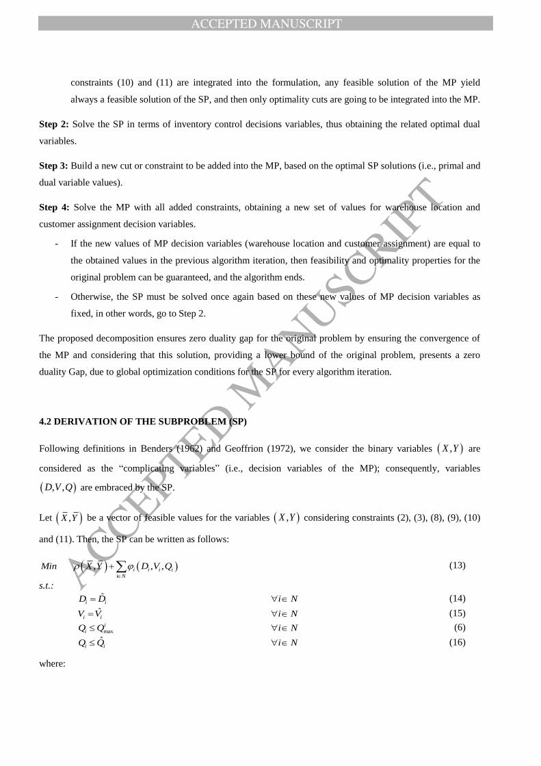
constraints (10) and (11) are integrated into the formulation, any feasible solution of the MP yield
always a feasible solution of the SP, and then only optimality cuts are going to be integrated into the MP.
Step 2: Solve the SP in terms of inventory control decisions variables, thus obtaining the related optimal dual
variables.
Step 3: Build a new cut or constraint to be added into the MP, based on the optimal SP solutions (i.e., primal and
dual variable values).
Step 4: Solve the MP with all added constraints, obtaining a new set of values for warehouse location and
customer assignment decision variables.
- If the new values of MP decision variables (warehouse location and customer assignment) are equal to
the obtained values in the previous algorithm iteration, then feasibility and optimality properties for the
original problem can be guaranteed, and the algorithm ends.
- Otherwise, the SP must be solved once again based on these new values of MP decision variables as
fixed, in other words, go to Step 2.
The proposed decomposition ensures zero duality gap for the original problem by ensuring the convergence of
the MP and considering that this solution, providing a lower bound of the original problem, presents a zero
duality Gap, due to global optimization conditions for the SP for every algorithm iteration.
4.2 DERIVATION OF THE SUBPROBLEM (SP)
Following definitions in Benders (1962) and Geoffrion (1972), we consider the binary variables ,X Y are
considered as the “complicating variables” (i.e., decision variables of the MP); consequently, variables
, ,D V Q are embraced by the SP.
Let ,X Y be a vector of feasible values for the variables ,X Y considering constraints (2), (3), (8), (9), (10)
and (11). Then, the SP can be written as follows:
, , ,i i i i
i N
Min X Y D V Q
(13)
s.t.:
ˆi iD D i N (14)
ˆi iV V i N (15)
max
i
iQ Q i N (6)
ˆi iQ Q i N (16)
where:

ACCEPTED MANUSCRIPT
ACCEPTED MANUSCRIP
T
, · ·i i ij ij
i N i N j M
X Y FC X AC Y
(17)
1, ,2
i i i ii i i i i i i
i
OC D HC QD V Q HC Z LT V
Q
(18)
ˆi ij j
j M
D Y d
(19)
ˆi ij j
j M
V Y v
(20)
1 1ˆ
i i i i iQ ICap X Z Z LT V (21)
According to equation (17), the first term in equation (13) represents the part of the total cost function in
equation (1), associated to the variables ,X Y and evaluated in ,X Y . For fixed values of variables ,X Y
this term becomes constant, and then the SP is solved without considering it. It is remarkable that this SP is
nonlinear and convex, although the original problem is nonconvex.
Notice that ,X Y may yield a feasible or an infeasible solution for the original problem (1)-(9). However,
given that constraints (10) and (11) are integrated into the problem formulation and also into the MP, always a
feasible solution can be found.
4.3 SOLVING THE SUBPROBLEM
Before to solve the SP, it is decoupled into a set of independent SPs, one SP for each warehouse i, SPi (i = 1,…,
N) as shown in (22). The same as the original SP, each SPi is of nonlinear, convex nature. These SPs are solved
analytically by inspection (or equivalently following Theil-Van de Panne conditions, 1960), as explained bellow.
Then optimal dual variables are determined based on a simple and direct application of the well know KKT
conditions.
max
, ,
. . :
ˆ
ˆ
ˆ
i i i i
i i
i i
i
i
i i
Min D V Q
s t
D D
V V
Q Q
Q Q
(22)
ACCEPTED MANUSCRIPT
ACCEPTED MANUSCRIP
T
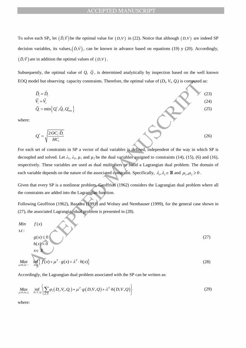
To solve each SPi, let ,D V be the optimal value for ,D V in (22). Notice that although ,D V are indeed SP
decision variables, its values, ˆ ˆ,D V , can be known in advance based on equations (19) y (20). Accordingly,
,D V are in addition the optimal values of ,D V .
Subsequently, the optimal value of Q, Q , is determined analytically by inspection based on the well known
EOQ model but observing capacity constraints. Therefore, the optimal value of (Di, Vi, Qi) is computed as:
ˆi i
D D (23)
ˆi iV V (24)
*
maxˆmin , , i
i i iQ Q Q Q (25)
where:
* 2· ·i i
i
i
OC DQ
HC (26)
For each set of constraints in SP a vector of dual variables is defined, independent of the way in which SP is
decoupled and solved. Let λ1, λ2, µ1 and µ2 be the dual variables assigned to constraints (14), (15), (6) and (16),
respectively. These variables are used as dual multipliers to build a Lagrangian dual problem. The domain of
each variable depends on the nature of the associated constraint. Specifically, 1 2, and
1 2, 0 .
Given that every SP is a nonlinear problem, Geoffrion (1962) considers the Lagrangian dual problem where all
the constraints are added into the Lagrangian function.
Following Geoffrion (1962), Bazaara (1993) and Wolsey and Nemhauser (1999), for the general case shown in
(27), the associated Lagrangian dual problem is presented in (28).
( )
. :
( ) 0
( ) 0
Min f x
s t
g x
h x
x X
(27)
0,
inf ( ) ( ) ( )T T
x XMax f x g x h x
(28)
Accordingly, the Lagrangian dual problem associated with the SP can be written as:
, ,0,inf , , · , , · , ,T T
i i i iD V Q
i N
Max D V Q g D V Q h D V Q
(29)
where:
ACCEPTED MANUSCRIPT
ACCEPTED MANUSCRIP
T
1
2
(30)
1
2
(31)
max
, , 0ˆ
i
Q Qg D V Q
Q Q
(32)
ˆ
, , 0ˆ
D Dh D V Q
V V
(33)
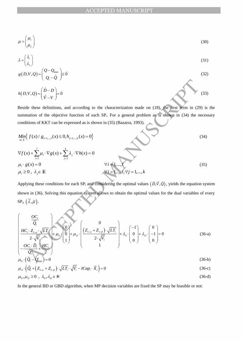
Beside these definitions, and according to the characterization made on (18), the first term in (29) is the
summation of the objective function of each SPi. For a general problem as is shown in (34) the necessary
conditions of KKT can be expressed as is shown in (35) (Bazarra, 1993).
1,..., 1,...,( ) / ( ) 0, ( ) 0i l j kx XMin f x g x h x
(34)
1 1
( ) ( ) ( ) 0
( ) 0 1,...,
0 , 1,..., , 1,...,
l k
i j
i j
i
i j
f x g x h x
g x i l
i l j k
(35)
Applying these conditions for each SPi and considering the optimal values , ,D V Q , yields the equation system
shown in (36). Solving this equation system allows to obtain the optimal values for the dual variables of every
SPi, , .
1 11
1 2 1 2
2
00 1 0
0 0 1 02 2
1 0 01
2
i
i
ii i
i i i i
i i
i i i
i
OC
Q
Z Z LTHC Z LT
V V
OC D HC
Q
(36-a)
1 max 0i
i iQ Q (36-b)
2 1 1 0i i i i i iQ Z Z LT V ICap X (36-c)
1 2 1 2, 0 , ,i i i i (36-d)
In the general BD or GBD algorithm, when MP decision variables are fixed the SP may be feasible or not:
ACCEPTED MANUSCRIPT
ACCEPTED MANUSCRIP
T
If the SP is feasible then there are two possible cases. The first case is when the SP has at least one
optimal and bounded solution, in which an optimality cut must be added into the MP. The second case
occurs when the SP is unbounded, case in which the algorithm ends due to the original problem is
unbounded too.
If the SP is infeasible then a feasibility cut must be added into the MP.
However, by adding constraints (10) and (11) to the MP the feasibility of each SPi is assured, and moreover each
SP is bounded. Thus, only optimality cuts are required to be added into the MP.
4.4 OPTIMALITY CUTS
Once the optimal primal and dual variables values , , , ,D V Q are obtained, as is shown in Section 4.3, it is
possible to generate an optimality cut to be added into the MP, as shown in (36), where Z is the objective
function of the MP.
1, max 2,
1 1 1
1, 2,
1 1
, , ,N N N
p p p p p i p p p
i i i i i i i i i i i
i i i
N Np p p p
i ij j i i ij j i
i j M i j M
Z X Y D V Q Q Q Q V ICap X
Y d D Y v V
(36)
Accordingly, the MP at each iteration k can be written as follow:
Min Z (37)
s.t.:
1ij
i N
Y j M
(2)
,ij iY X i N j M (3)
1,
1
2, 1, max
1
2,
1
, , , ·N
p p p p p
i i i i ij j i
i j M
Np p p p i k
i ij j i i i
i j M
Np p p
i i i i i i
i
Z X Y D V Q Y d D
Y v V Q Q p P
Q V ICap X
(38)
0,1iX i N (8)
0,1 ,ijY i N j M (9)
The set Pk in (38) represents the set of cuts obtained and added into the MP after k algorithm iterations. For the
initial iteration 0kP , and the MP is unbounded Z . Thus, an auxiliary optimization problem is built

ACCEPTED MANUSCRIPT
ACCEPTED MANUSCRIP
T
and solved to generate an initial MP feasible solution and to start the algorithm, as described in the following
section.
5. COMPUTATIONAL IMPLEMENTATION AND RESULTS
The computational application of the proposed approach was made considering 160 instances. These instances
were created from 5 base instances. From each one of these 5 base instances, 32 instances with different sizes
were created. Base instances were generated from a random distribution in a square area of 2000[km] of side.
Every base instance considers 20 potential sites to install a warehouse and the location of 40 customers. The
instances were named using the following notation N_M_I, where: N represents the number of potential
warehouses, M represents the number of customers and I the number of the base instance. The parameter N takes
values in {5, 10, 15, 20}, M takes values in {5, 10, 15, 20, 25, 30, 35, 40} and finally I takes values in {1, 2, 3, 4,
5}.
The initial solution for the algorithm is obtained using a basic Facility Location Problem, where two sets of
constraints are integrated to ensure SPs feasibility. The model uses the MP variables ,X Y and a subset of
parameters from the original model. The mathematical formulation is as follows:
( , )
,X Y
X YMin (17)
s.t.:
1ij
i N
Y j M
(2)
,ij iY X i N j M (3)
max
1
·M
i
ij jj
Y v V i N
(10)
1
M
i ijj
X Y i N
(11)
0,1iX i N (8)
0,1 ,ijY i N j M (9)
The objective function (17) is sum of warehouses settings and assignment costs. Sets of constraints (2), (3), (8)
and (9) are the same as in the original model. Constraints (10) and (11) are derived from the original constraints
(7) and the definition made on (12). Constraints are valid inequalities to ensure that a warehouse is open only if
at least one customer is assigned to it.
The proposed algorithm is implemented in Microsoft Visual C++ 2010, and MP is solved using Cplex 12.5, both
using a computer with a processor Intel Core I7 of 3.4 GHz and 8 GB of RAM in a 64-bit Operating System.

ACCEPTED MANUSCRIPT
ACCEPTED MANUSCRIP
T
The notation of the results is showed in the Table 1.
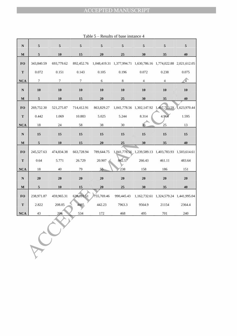
The following tables show the results for each base instance. Tables 2-6 show the results obtained for each base
instance, the optimal solution was reached for each and every of these 160 instances.
Analyzing the Tables 2-6 it is possible to get insights about the behavior of the solutions. In a specific column
the number of customers is fixed but going down 5 more potential warehouses are added in each instance, from 5
to 20. Thus, each feasible solution of an instance is also feasible in all the instances bellow for the same column.
Having in mind that the optimal solution is found for all the instances, this value is in fact an upper-bound for the
optimal value for all the instances bellow in the same column. Moreover, in some cases the optimal solution of
an instance is also optimal for some of the instances bellow (e.g. instances 10_5_1, 15_5_1 and 20_5_1).
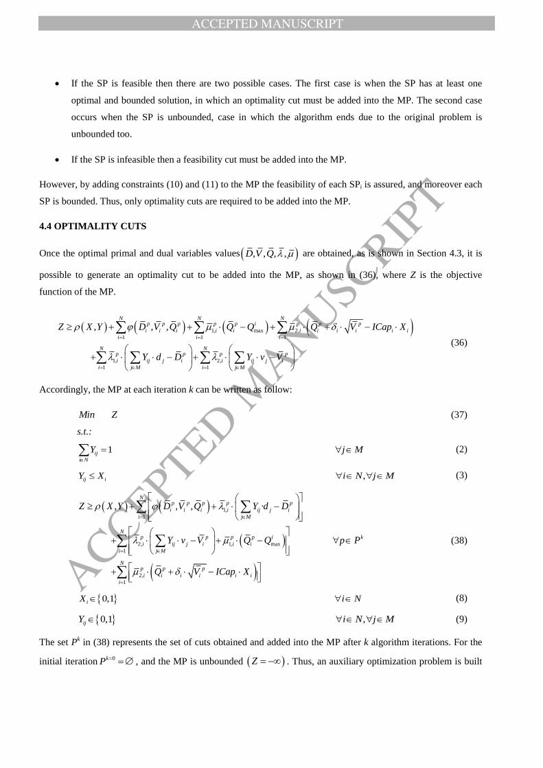
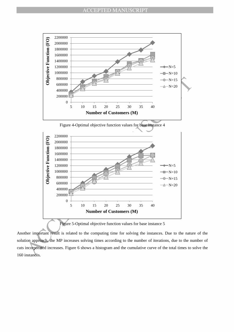
Figures 1 - 5 show the behavior of the optimal objective function for each group of instances associated to each
base instance. The optimal objective function value for a fixed number of potential warehouses performs a non-
decreasing behavior when the number of customers is increased. In most cases the curve for an instance tends to
show a linear growth. Nevertheless, in some cases adding five customers generate a marginal increase between
the optimal objective function values of the instances (e.g. optimal values of instances 10_35_5 and 10_40_5).
Figure 1-Optimal objective function values for base instance 1
0
200000
400000
600000
800000
1000000
1200000
1400000
1600000
1800000
2000000
2200000
5 10 15 20 25 30 35 40
Ob
ject
ive
Fu
nct
ion
(F
O)
Number of Customers (M)
N=5
N=10
N=15
N=20

ACCEPTED MANUSCRIPT
ACCEPTED MANUSCRIP
T
Figure 2-Optimal objective function values for base instance 2
Figure 3-Optimal objective function values for base instance 3
0
200000
400000
600000
800000
1000000
1200000
1400000
1600000
1800000
2000000
2200000
5 10 15 20 25 30 35 40
Ob
ject
ive
Fu
nct
ion
(F
O)
Number of Customers (M)
N=5
N=10
N=15
N=20
0
200000
400000
600000
800000
1000000
1200000
1400000
1600000
1800000
2000000
2200000
5 10 15 20 25 30 35 40
Ob
ject
ive
Fu
nct
ion
(F
O)
Number of Customers (M)
Series1
Series2
Series3
Series4
ACCEPTED MANUSCRIPT
ACCEPTED MANUSCRIP
T
Figure 4-Optimal objective function values for base instance 4
Figure 5-Optimal objective function values for base instance 5
Another important result is related to the computing time for solving the instances. Due to the nature of the
solution approach, the MP increases solving times according to the number of iterations, due to the number of
cuts incorporated increases. Figure 6 shows a histogram and the cumulative curve of the total times to solve the
160 instances.
0
200000
400000
600000
800000
1000000
1200000
1400000
1600000
1800000
2000000
2200000
5 10 15 20 25 30 35 40
Ob
ject
ive
Fu
nct
ion
(F
O)
Number of Customers (M)
N=5
N=10
N=15
N=20
0
200000
400000
600000
800000
1000000
1200000
1400000
1600000
1800000
2000000
2200000
5 10 15 20 25 30 35 40
Ob
ject
ive
Fu
nct
ion
(F
O)
Number of Customers (M)
N=5
N=10
N=15
N=20

ACCEPTED MANUSCRIPT
ACCEPTED MANUSCRIP
T
Figure 6-Histogram of computing times.
Analyzing Figure 6, it is observed that most of the instances are solved in less than an hour (86.875% of the
instances). According to Table 7 it is possible to notice that an 80.6% of the instances are solved in less than ten
minutes. Moreover, the 67.5% of the instances need less than one minute to be solved.
Considering the nature of the proposed solution approach it may be relevant to analyze the relation between
computing times and the number of cuts added into the MP. Figure 7 shows the behavior of computing times
according to the number of cut added (NCA) for the 160 instances, putting aside the impact of the specific
instance characteristics (e.g. number of warehouses, numbers of customers).
Figure 7-Relationship between NCA and total time
0
20
40
60
80
100
120
140
160
1 2 3 4 5 6 7 8 9 101112131415161718192021222324252627
Nu
mb
er o
f in
sta
nce
s
Total Time [Hour]
y = 4E-05x3 + 0.0169x2 + 1.1637x
R² = 0.9471
0
10000
20000
30000
40000
50000
60000
70000
80000
90000
100000
0 200 400 600 800 1000 1200
To
tal
Tim
e [s
]
NCA

ACCEPTED MANUSCRIPT
ACCEPTED MANUSCRIP
T
According to Figure 7 it is possible to identify a strong relationship that explains the computing time by the
number of cuts added, with a more accentuated tendency than linear. Naturally, there is more characteristic that
should be considered for a better understanding of this relationship (e.g. number of potential warehouses,
number of customer, spatial distribution).
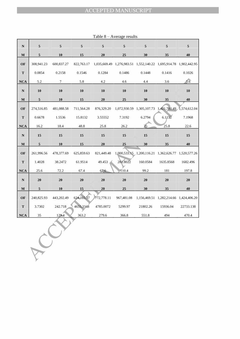
Finally, Table 8 summarizes the previous results by averaging the results of the five base instances. In order to
isolate the effect of the size of the instances the average is made considering the instances with the same number
of potential warehouses and customers.
The average values of optimal objective function, total time and the number of cuts added into the MP are
presented in Figure 8, 9 and 10 respectively.
Figure 8-Optimal objective function values for average results
As expected, Figure 8 confirms the same behavior of the optimal values for each base instance.
0
200000
400000
600000
800000
1000000
1200000
1400000
1600000
1800000
2000000
5 10 15 20 25 30 35 40
Ob
ject
ive
Fu
nct
ion
(F
O)
Number of Customers (M)
N=5
N=10
N=15
N=20

ACCEPTED MANUSCRIPT
ACCEPTED MANUSCRIP
T
Figure 9-Total times for average results
Analyzing Figure 9 it is possible to visualize that the computing times for instances with 20 potential warehouses
are notably greater that other instances with lower values of N. Moreover, solving times of the other instances
tend to be relatively low, especially highlighting the global optimality ensured with the proposed solution
approach.
Figure 10-Number of cuts added for average results
In general terms, the behavior showed in Figure 10 it is similar to the performance of total times in Figure 9. It is
clearly observed that the instances with more cuts are those with 20 potential warehouses. By contrasting the
information obtained from Figure 9 and 10, it is possible to observe that the number of cuts added it is strongly
0
5000
10000
15000
20000
25000
5 10 15 20 25 30 35 40
Av
era
ge
To
tal
Tim
e [s
]
Number of Customers (M)
N=5
N=10
N=15
N=20
0
100
200
300
400
500
600
5 10 15 20 25 30 35 40
Av
era
ge
NC
A
Number of Customers (M)
N=5
N=10
N=15
N=20

ACCEPTED MANUSCRIPT
ACCEPTED MANUSCRIP
T
related to the total time needed to solve all instance as previously suggested by Figure 7. This insight suggests
further research focused on reducing the number of cuts.
6. CONCLUSIONS AND FUTURE WORK
This paper studied a joint Inventory Location Problem with Stochastic Inventory Capacity Constraints, which
considers decisions related to both the structure of the supply chain network and the sizing of inventories at each
allocated warehouse. As a consequence, the mathematical structure of the studied mixed integer nonlinear
nonconvex programming problem requires efficient solution approaches for obtaining optimal solutions in
competitive times. Accordingly, this paper proposes a novel Generalized Benders Decomposition based solution
approach that ensures optimality. It is remarkable that, despite of nonconvex model structure, the proposed
solution approach ensures global optimality.
Due to this study is focused on long term optimization models, whose usage is sporadic, computing times can be
considered not as important as the quality of the solutions. In other words, computing times can be longer than
for real time or short term optimization problem. However, the time for solving the problem is a relevant
performance indicator to classify an algorithmic approach. It is remarkable that for the real world based medium
sized instances considered in this study, 75% of the instances were solved in less than four minutes, especially
considering the complexity of the model. The sizes of the employed instances can be considered as
medium/small. However, these instances may represent real world sizes for specific industry or company cases.
The proposed solution approach introduces an interesting and novel strategy to decompose the problem based on
the decomposition scheme of GBD. Setting the binary variables as the MP decision variables yields a set of SPs
that can be analytically solved at optimality. As a consequence, the Lagrangian dual information is obtained
using closed mathematical expressions, and it is properly employed to build the cuts to be added iteratively into
the MP. Furthermore, the MPs can be solved at optimality using a standard commercial solver, given its mixed
integer linear programming nature. Then the proposed strategy deals with the nonconvexity of the original
problem and ensures global optimality.
In terms of future research, it worth to be mentioned the application of the proposed solution approach to other
inventory location problems, considering other inventory control policies, more complex supply chain, or
considering other type of constraints. Moreover, the model can be adapted to deal with unique features and
requirements of specific industries and/or type of commodities (e.g. final products, raw materials, spare parts).
The existence of more extended supply chain networks, where sub-networks are embedded into a common
shared network, may lead to the use of nested decomposition approaches. Natural extensions are multi-period
and multi-commodity formulations, then increasing the applicability of the ILP models on real industrial cases.
However, these formulations rely on an even higher complexity in terms of their resolution. Considering the
results observed in this paper, the proposed decomposition increase potentiality of GBD based approaches for

ACCEPTED MANUSCRIPT
ACCEPTED MANUSCRIP
T
these more complex ILPs models. Further important issues are potential enhancements to the proposed algorithm
in order to improve the general performance of the algorithm such as computational aspects and also algorithmic
design issues (e.g. lazy constraints, convergence criteria and approaches for solving the MP).
AKNOLEDGMENTS
This research has been partially supported by: the Agreement of Performance for Higher Regional Education,
initiative executed by Pontificia Universidad Católica de Valparaiso (PMI-PUCV); SustainOwner (“Sustainable
Design and Management of Industrial Assets through Total Value and Cost of Ownership"), a project sponsored
by the EU Framework Programme Horizon 2020, MSCA-RISE-2014: Marie Skłodowska-Curie Research and
Innovation Staff Exchange (RISE), grant agreement number 645733-Sustain-Owner- H2020-MSCA-RISE-2014.
The authors want to express their gratitude for this support.
ACCEPTED MANUSCRIPT
ACCEPTED MANUSCRIP
T
REFERENCES
Ağrahm S., Geunes, J., Taşkin, Z.C. (2012). A facility location model with safety stock costs: analysis of the
cost of single-sourcing requirements. Journal of Global Optimization, 54, 551-581.
Amiri-Aref, M., Klibi, W., Babai, M.Z. (2017). The multi-sourcing location inventory problem with stochastic
demand. European Journal of Operational Research, In Press. 2017. doi: 10.1016/j.ejor.2017.09.003
Bazaraa, M.S., Sherali, H.D., Shetty, C.M. (1993). Nonlinear Programming: Theory and Algorithms, Second
Edition. New York, NY: Wiley.
Bradley, J.R., Arnzten, B.C. (1999). The Simultaneous Planning of Production, Capacity, and Inventory in
Seasonal Demand Environments. Operations Research, 47(6), 795-806.
Benders, J.F. (1962). Partitioning procedures for solving mixed-variables programming problems. Numerische
Mathematik, 4, 238-252.
Bertsekas, D.P. (1999). Nonlinear Programming, Second Edition, Cambridge: Athena Scientific.
Bitran, G.R., Hass, E.A., Hax, A.C. (1982). Hierarchical Production Planning: A Single Stage System.
Operations Research, 29(4), 717-743.
Bitran, G.R., Hass, E.A., Hax, A.C. (1982). Hierarchical Production Planning: A Two-Stage System. Operations
Research, 30(2), 232-251.
Cabrera, G., Miranda, P.A., Cabrera, E., Soto, R., Crawford, B., Rubio, J.M., Paredes, F. (2013). Solving a
Novel Inventory Location Model with Stochastic Constraints and (R,s,S) Inventory Control Policy.
Mathematical Problems in Engineering, 2013. doi:10.1155/2013/670528
Caniato, F., Kalchschmidt, M., Ronchi, S., Verganti, R., Zotteri, G. 2005. Clustering Customers to Forecast
Demand. Production Planning & Control, 16(1), 32-43.
Chase, R.B., Jacobs, R., Aquilano, N.J. (2004). Operations Management for Competitive Advantages. New
York, NY: McGraw Hill.
Costa, A. (2005). A survey on Benders decomposition applied to fixed-charge network design problems.
Computers & Operations Research, 32, 1429-1450.
Coyle, J.J., Bardi, E.J., Langley, C.J. (2003). The Management of Business Logistics: A Supply Chain
Perspective. Quebec: Transcontinental Louisville.
ACCEPTED MANUSCRIPT
ACCEPTED MANUSCRIP
T
Coyle, J.J., Langley, C.J., Novack, R.A., Gibson, B. (2009). Supply Chain Management: A Logistic Perspective.
Mason, OH: South-Western Cengage Learning.
Current, J.R., and Schilling, D.A. (1990). Analysis of Errors Due to Demand Data Aggregation in the Set
Covering and Maximal Covering Location Problems. Geographical Analysis Volume 22(2), 116-126.
Daskin, M.S. (1995). Network and Discrete Location: Models, Algorithms, and Applications, New York, NY:
Wiley-Interscience.
Daskin M.S., Coullard C.R., Max Shen Z.J. (2002). An Inventory-location Model: Formulation, Solution
Algorithm and Computational Results. Annals of Operations Research, 110(1), 83-106.
Diabat, A., Battaïa, O., Nazzal, D. (2015). An improved Lagrangian relaxation-based heuristic for a joint
location-inventory problem. Computers & Operations Research, 61, 170-178.
Drezner, T. 2014. A review of competitive facility location in the plane. Logistic Research, 7(114), 1-12.
Drezner, Z., Hamacher, H. W. (2002). Facility Location: Applications and Theory. New York, NY: Springer-
Verlag.
Eiselt, H.A., Marianov, V. (2011) Foundations of Location Analysis. New York, NY: Springer.
Eiselt, H.A., Marianov, V. (2015) Applications of Location Analysis. New York, NY: Springer.
Emir-Farinas, H., Francis, R.L. (2005). Demand point aggregation for planar covering location models. Annals
of Operations Research. 136(1), 175-192.
Erlebacher, S.J., Meller, R.D. (2000). The interaction of location and inventory in designing distribution
systems. IIE Transactions, 32(2), 155-166.
Escalona, P., Ordonez, F., Marianov, V. (2015). Joint location-inventory problem with differentiated service
levels using critical level policy. 83, 141-157.
Fahimnia, B. Parkinson, E. Rachaniontis, N.P., Mohamed, Z. Goh, M. (2013). Supply chain planning for a
multinational enterprise: A performance analysis case study. International Journal of Logistics Research and
Applications, 16(5), 349-366.
Farahani, R.Z., Rashidi Bajgan, H., Fahimnia, B. Kaviani, M. (2015). Location-inventory problem in supply
chains: a modeling review. International Journal of Production Research, 53(12), 3769-3788.

ACCEPTED MANUSCRIPT
ACCEPTED MANUSCRIP
T
Farahani, R.Z., Rezapour, S., Drezner, T., Fallah, S. (2014). Competitive supply chain network design: An
overview of classifications, models, solution techniques and applications. Omega, 45, 92-118.
Francis, R.L., Lowe, T.J., Tamir, A., Emir-Farinas, H. (2004). A framework for demand point and solution space
aggregation analysis for location models. European Journal of Operational Research, 159 (3), 574-585.
Fontalvo, M.O. Maza, V.C., Miranda, P.A. (2017). A Meta-Heuristic Approach to a Strategic Mixed Inventory-
Location Model: Formulation and Application. Transportation Research Procedia, 25, 729-746.
Geoffrion, A.M. (1972). Generalized Benders Decomposition. Journal of Optimization Theory and Applications
Volume 10(4), 237-260.
Ghiani, G., Laporte, G., Musmanno R. (2004). Introduction to Logistics Systems Planning and Control. New
York, NY: Wiley.
Ghorbani, A., Akbari Jokar, M.A. (2016). A hybrid imperialist competitive-simulated annealing algorithm for a
multisource multi-product location-routing-inventory problem, 101, 116-127.
Guerrero, W.J., Prodhon, C., Velasco, N., Amaya, C.A. (2013). Hybrid heuristic for the inventory location-
routing problem with deterministic demand. International Journal of Production Economics, 146, 359-370.
Harris, F.W. (1913), How many parts to make at once. Factory, the Magazine of Management, 10(2), 135-136.
Hax, A.C., Candea, D. (1984). Production and Inventory Management. New Jersey, NJ: Prentice Hall.
Hillier, F.S., Lieberman, G.J. (2005). Introduction to Operations Research. New York, NY: McGraw Hill.
Jayaraman, V. (1998). Transportation, facility location and inventory issues in distribution network design: An
investigation. International Journal of Operations and Production Management, 18(5), 471-494.
Li, X., Tomasgard, A., Barton, P.I. (2011). Nonconvex Generalized Benders Decomposition for Stochastic
Separable Mixed-Integer Nonlinear Programs. Journal of Optimization Theory and Applications, 151(3), 425-
454.
Li, X., Sundaramoorthy, A., Barton, P.I. (2014). Nonconvex Generalized Decomposition. In: Rassias, T.M.,
Floudas, C.A., Butenko, S. (Eds), Optimization in Science and Engineering (307-331). New York, NY: Springer.
Melo, M.T., Nickel, S., Saldanha-da-Gama, F. (2009). Facility location and supply chain management-A review.
European Journal of Operational Research, 196, 401-412.
ACCEPTED MANUSCRIPT
ACCEPTED MANUSCRIP
T
Miranda, P.A., Garrido, R.A. (2004). Incorporating inventory control decisions into a strategic distribution
network design model with stochastic demand. Transportation Research Part E: Logistics and Transportation
Review, 40(3), 183-207.
Miranda, P.A., Garrido, R.A. (2006). A Simultaneous Inventory Control and Facility Location Model with
Stochastic Capacity Constraints. Networks and Spatial Economics, 6(1), 39-53.
Miranda, P.A., Garrido, R.A. (2008). Valid inequalities for Lagrangian relaxation in a inventory location
problem with stochastic capacity. Transportation Research, Part E, 44, 47-65.
Miranda, P.A., Garrido, R.A. (2009). Inventory service-level optimization within distribution network design
problem. International Journal of Production Economics, 122, 276-285.
Miranda, P.A., Cabrera, G. (2010). Inventory location problem with stochastic capacity constraints under
periodic review (R,s,S). International Conference on Industrial Logistics “Logistics and Sustainability”, 1, 289-
296.
Mourtis, M., Evers, J.J.M. (1995). Distribution network design: An integrated planning support framework.
International Journal of Physical Distribution & Logistics Management, 25(5), 43-57.
Nekooghadirli, N., Tavakkoli-Moghaddam, Ghezavati, V.R., Javanmard, S. (2014). Solving a new bi-objective
location-routing-inventory problem in a distribution network by meta-heuristics. Computers & Industrial
Engineering, 76, 204-221.
Owen, S.H., Daskin, M.S. (1998) Strategic facility location: A review. European Journal of Operational
Research, 111(3), 423-447.
Ozsen, L., Coullard, C., Daskin, M. (2008). Capacitated warehouse location model with risk pooling. Naval
Research Logistics, 55(4), 295-312.
Ozsen, L., Daskin, M.S., Coullard, C. (2009). Facility Location Modeling and Inventory Management with
Multisourcing. Transportation Science, 43(4), 455-472.
Pereira, V., Costa, H.G. (2014). A literature review on lot size with quantity discounts: 1995-2013. Journal of
Modelling in Management, 10(3), 341-359.
Perez-Loaiza, R.E., Olivares-Benitez, E., Miranda, P.A., Guerrero, A., Martinez, J.L. (2017). Supply chain
network design with efficiency, location, and inventory policy using a multiobjective evolutionary algorithm.
International Transactions in Operational Research, 24, 251-275.
ACCEPTED MANUSCRIPT
ACCEPTED MANUSCRIP
T
Pourhejazy, P., Kwon, O.K. (2016). The New Generation of Operations Research Methods in Supply Chain
Optimization: A review. Sustainability, 8(10), 1033. doi:10.3390/su8101033. Retrieved from:
http://www.mdpi.com/2071-1050/8/10/1033/pdf.
Rahmaniani, R., Crainic, T.G., Gendreau, M, Rei, W. (2017). The Benders decomposition algorithm: A literature
review. European Journal of Operational Research, 259(3), 801-817.
Ross, A., Khajehnezhad, M., Otieno, W., Aydas, O. (2017). Integrated location-inventory modelling under
forward and reverse product flows in the used merchandise retail sector: A multi-echelon formulation. European
Journal of Operational Research, 259(2), 664-676.
Schuster, M., Tancrez, J.S. (2017). A heuristic algorithm for solving large location-inventory problems with
demand uncertainty. European Journal of Operational Research, 259(2), 413-423.
Shen, Z.J. (2007). Integrated Supply Chain Design Models: A Survey and Future Research Directions. Journal of
Industrial and Management Optimization, 3(1), 1-27.
Shen, Z.J., Coullard, C., Daskin, M. (2003). A joint location-inventory model. Transportation Science, 37 (1),
40-55.
Simchi-Levi, D., Kaminsky, P., Simchi-Levi, E. (2003). Designing and Managing the Supply Chain: Concepts,
Strategies and Case Studies. New York, NY: McGraw-Hill.
Simchi-Levi, D., Kaminsky, P., Simchi-Levi, E. (2004). Managing the Supply Chain: The Definitive Guide for
the Bussiness Professional. New York, NY: McGraw-Hill.
Snyder, L. (2006). Facility location under uncertainty: a review. IIE Transactions, 38, 537-554.
Snyder, L., Daskin, M.S., Teo, C.P. (2007). The stochastic location model with risk pooling. European Journal of
Operational Reseach, 179, 1221-1238.
Tavakkoli-Moghaddam, R., Raziei, Z. (2016). A New Bi-Objective Location Routing-Inventory Problem with
Fuzzy Demands. IFAC-PaperOnLine, 49(12), 1116-1121.
Theil, H., Van de Panne, C. (1960). Quadratic Programming as an Extension of Classical Quadratic
Maximization. Management Science, 7, 1-20.
Wheatley, D., Gzara, F., Jewkes, E. (2015). Logic-based Benders decomposition for an inventory-location
problem with service constraints. Omega, 55, 10-23.

ACCEPTED MANUSCRIPT
ACCEPTED MANUSCRIP
T
Wolsey, L.A., Nemhauser, G.L. (1999). Integer and Combinatorial Optimization. New York, NY: Willey.
Zhang, Y., Qi, M., Miao, L., Liu, E. (2014). Hybrid metaheuristic solutions to inventory location routing
problem. Transportation Research Part E, 70, 305-323.
ACCEPTED MANUSCRIPT
ACCEPTED MANUSCRIP
T
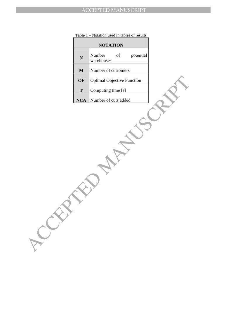
Table 1 – Notation used in tables of results
NOTATION
N Number of potential
warehouses
M Number of customers
OF Optimal Objective Function
T Computing time [s]
NCA Number of cuts added

ACCEPTED MANUSCRIPT
ACCEPTED MANUSCRIP
T
Table 2 – Results of base instance 1
N 5 5 5 5 5 5 5 5
M 5 10 15 20 25 30 35 40
OF 282,336.24 554,434.37 770,046.77 957,136.84 1,242,964.02 1,578,384.49 1,583,497.47 1,836,125.71
T 0.144 0.088 0.089 0.046 0.212 0.142 0.048 0.052
NCA 7 6 5 3 5 6 3 3
N 10 10 10 10 10 10 10 10
M 5 10 15 20 25 30 35 40
OF 268,123.24 466,713.86 657,455.23 843,767.27 1,006,153.99 1,227,083.68 1,363,669.12 1,575,606.95
T 0.455 0.288 1.457 3.163 1.126 2.149 4.646 5.569
NCA 13 9 22 31 16 16 28 29
N 15 15 15 15 15 15 15 15
M 5 10 15 20 25 30 35 40
OF 268,123.24 466,713.86 571,136.42 785,754.97 951,789.76 1,154,815.38 1,316,919.51 1,536,874.27
T 1.075 6.631 0.859 46.581 57.811 96.095 394.99 780.43
NCA 26 47 13 91 90 97 156 203
N 20 20 20 20 20 20 20 20
M 5 10 15 20 25 30 35 40
OF 268,123.24 449,567.32 558,464.41 748,307.26 951,789.76 1,118,771.67 1,240,319.96 1,396,095.90
T 4.271 12.715 5.374 48.736 716.95 1164.6 1810.9 392.59
NCA 52 52 27 80 181 211 246 115

ACCEPTED MANUSCRIPT
ACCEPTED MANUSCRIP
T
Table 3 – Results of base instance 2
N 5 5 5 5 5 5 5 5
M 5 10 15 20 25 30 35 40
FO 273,509.31 488,596.29 728,109.15 971,747.72 1,202,002.78 1,352,426.42 1,650,183.90 1,847,962.81
T 0.065 0.127 0.24 0.099 0.128 0.113 0.12 0.109
NCA 3 4 5 3 3 3 3 3
N 10 10 10 10 10 10 10 10
M 5 10 15 20 25 30 35 40
FO 249,114.18 440,739.38 698,268.74 816,057.92 1,058,996.82 1,259,315.81 1,382,592.91 1,545,264.18
T 1.252 1.708 50.601 2.143 17.514 13.621 8.593 21.432
NCA 18 20 81 15 39 36 22 44
N 15 15 15 15 15 15 15 15
M 5 10 15 20 25 30 35 40
FO 234,623.95 440,739.38 633,728.35 777,430.84 957,822.21 1,152,265.98 1,314,181.59 1,527,322.99
T 2.227 76.867 224.59 79.18 178.72 225.44 267.04 5984.9
NCA 29 88 127 69 99 96 96 304
N 20 20 20 20 20 20 20 20
M 5 10 15 20 25 30 35 40
FO 217,304.71 412,105.94 633,294.85 777,430.84 937,273.62 1,152,265.98 1,283,385.74 1,459,502.27
T 7.109 221.75 12201 16428 1939.5 67309 38639 95420
NCA 32 124 470 580 283 1103 805 1101

ACCEPTED MANUSCRIPT
ACCEPTED MANUSCRIP
T
Table 4 – Results of base instance 3
N 5 5 5 5 5 5 5 5
M 5 10 15 20 25 30 35 40
FO 309,773.67 663,268.42 857,475.38 1,134,696.25 1,324,234.81 1,696,998.56 1,792,011.57 1,933,157.61
T 0.082 0.63 0.172 0.312 0.156 0.313 0.243 0.125
NCA 4 12 4 6 4 5 5 4
N 10 10 10 10 10 10 10 10
M 5 10 15 20 25 30 35 40
FO 267,418.10 496,809.74 700,722.82 891,762.16 1,087,393.04 1,353,302.51 1,404,540.69 1,574,895.32
T 0.784 4.483 1.504 1.941 10.119 5.058 4.099 6.685
NCA 15 31 16 12 26 20 17 19
N 15 15 15 15 15 15 15 15
M 5 10 15 20 25 30 35 40
FO 244,661.41 492,831.52 613,697.72 841,690.07 1,014,224.90 1,242,187.28 1,415,749.10 1,481,751.09
T 1.31 92.139 52.678 60.781 300.86 196.6 7006.6 473.58
NCA 20 135 78 61 96 106 404 139
N 20 20 20 20 20 20 20 20
M 5 10 15 20 25 30 35 40
FO 223,911.16 459,349.51 613,697.72 776,053.35 971,087.48 1,206,745.15 1,291,004.46 1,426,955.46
T 2.829 763.36 1966 6857.7 8617.6 25254 6300.3 9579.7
NCA 17 220 270 450 367 492 244 508
ACCEPTED MANUSCRIPT
ACCEPTED MANUSCRIP
T
Table 5 – Results of base instance 4
N 5 5 5 5 5 5 5 5
M 5 10 15 20 25 30 35 40
FO 343,840.59 693,779.62 892,452.76 1,048,419.31 1,377,994.71 1,630,786.16 1,774,022.88 2,021,612.05
T 0.072 0.151 0.143 0.105 0.196 0.072 0.238 0.075
NCA 7 7 7 6 8 4 4 4
N 10 10 10 10 10 10 10 10
M 5 10 15 20 25 30 35 40
FO 269,752.30 521,275.87 714,412.91 863,829.27 1,041,778.56 1,302,147.92 1,417,713.59 1,623,970.44
T 0.442 1.069 10.883 5.025 5.244 8.314 4.964 1.595
NCA 18 24 58 38 30 36 25 13
N 15 15 15 15 15 15 15 15
M 5 10 15 20 25 30 35 40
FO 245,527.63 474,834.38 663,728.94 789,644.75 1,041,778.56 1,239,589.13 1,403,783.93 1,503,614.61
T 0.64 5.771 26.729 20.907 862.57 266.43 461.11 483.64
NCA 18 40 79 55 238 158 186 151
N 20 20 20 20 20 20 20 20
M 5 10 15 20 25 30 35 40
FO 238,971.87 459,965.31 639,091.51 755,769.46 990,445.43 1,162,732.61 1,324,579.24 1,441,995.04
T 2.822 208.05 4485 442.23 7963.3 9564.9 21154 2364.4
NCA 43 208 534 172 468 495 701 240

ACCEPTED MANUSCRIPT
ACCEPTED MANUSCRIP
T
Table 6 – Results of base instance 5
N 5 5 5 5 5 5 5 5
M 5 10 15 20 25 30 35 40
FO 335,246.32 604,107.67 865,731.80 1,066,347.32 1,237,721.23 1,502,105.47 1,679,858.10 1,873,356.59
T 0.064 0.083 0.129 0.08 0.051 0.084 0.059 0.152
NCA 5 6 8 3 3 4 3 4
N 10 10 10 10 10 10 10 10
M 5 10 15 20 25 30 35 40
FO 318,176.43 479,904.04 786,961.71 966,229.42 1,170,330.56 1,383,688.76 1,539,986.14 1,553,323.32
T 0.406 0.22 14.621 5.5056 2.593 2.255 8.274 0.703
NCA 17 8 67 33 20 17 37 8
N 15 15 15 15 15 15 15 15
M 5 10 15 20 25 30 35 40
FO 317,046.57 479,904.04 647,006.72 912,726.76 1,037,050.31 1,211,723.26 1,362,499.71 1,553,323.32
T 1.762 9.828 4.901 39.816 9.05 15.727 49.544 689.93
NCA 35 51 40 62 29 39 63 192
N 20 20 20 20 20 20 20 20
M 5 10 15 20 25 30 35 40
FO 255,818.67 435,024.37 647,006.72 806,329.66 986,809.08 1,141,832.15 1,271,783.91 1,397,482.35
T 1.62 7.715 4619.3 148.37 7262.5 5718.8 11776 5909
NCA 31 43 515 116 535 458 474 388

ACCEPTED MANUSCRIPT
ACCEPTED MANUSCRIP
T
Table 7 – Computational times
Time [s]
Number of
instances
Percentage
[%] Cumulative
Cumulative
Percentage [%]
T 1 49 30.6% 49 30.6
1 T 10 42 26.3% 91 56.9
10 T 60 17 10.6% 108 67.5
60 T 300 14 8.8% 122 76.3
300 T 600 7 4.4% 129 80.6
600 T 1,800 6 3.8% 135 84.4
1,800 T 3,600 10 6.3% 139 86.9
3,600 T 18,000 16 10.0% 155 96.9
18,000 T 36,000 2 1.3% 157 98.1
36,000 T 3 1.9% 160 100.0
ACCEPTED MANUSCRIPT
ACCEPTED MANUSCRIP
T
Table 8 – Average results
N 5 5 5 5 5 5 5 5
M 5 10 15 20 25 30 35 40
OF 308,941.23 600,837.27 822,763.17 1,035,669.49 1,276,983.51 1,552,140.22 1,695,914.78 1,902,442.95
T 0.0854 0.2158 0.1546 0.1284 0.1486 0.1448 0.1416 0.1026
NCA 5.2 7 5.8 4.2 4.6 4.4 3.6 3.6
N 10 10 10 10 10 10 10 10
M 5 10 15 20 25 30 35 40
OF 274,516.85 481,088.58 711,564.28 876,329.20 1,072,930.59 1,305,107.73 1,421,700.49 1,574,612.04
T 0.6678 1.5536 15.8132 3.55552 7.3192 6.2794 6.1152 7.1968
NCA 16.2 18.4 48.8 25.8 26.2 25 25.8 22.6
N 15 15 15 15 15 15 15 15
M 5 10 15 20 25 30 35 40
OF 261,996.56 478,377.69 625,859.63 821,449.48 1,000,533.15 1,200,116.21 1,362,626.77 1,520,577.26
T 1.4028 38.2472 61.9514 49.453 281.8022 160.0584 1635.8568 1682.496
NCA 25.6 72.2 67.4 67.6 110.4 99.2 181 197.8
N 20 20 20 20 20 20 20 20
M 5 10 15 20 25 30 35 40
OF 240,825.93 443,202.49 624,165.37 772,778.11 967,481.08 1,156,469.51 1,282,214.66 1,424,406.20
T 3.7302 242.718 4655.3348 4785.0072 5299.97 21802.26 15936.04 22733.138
NCA 35 129.4 363.2 279.6 366.8 551.8 494 470.4