A generalized algorithm for determining pair-wise ...ncss-tech.github.io/AQP/presentations/AQP-num_soil_classification.pdf · A generalized algorithm for determining pair-wise dissimilarity

A generalized algorithm for determiningpair-wise dissimilarity between soil profiles

D.E. Beaudette, P. Roudier, A.T. O’Geen

USDA-NRCS Sonora, CALandcare Research, NZ

University of California Davis, CA

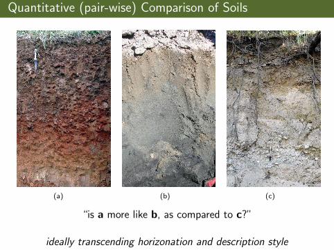
Quantitative (pair-wise) Comparison of Soils

(a) (b) (c)

“is a more like b, as compared to c?”

ideally transcending horizonation and description style

Numerical Soil Classification

essentially: an evaluation of “distance” in property space

reminder: those who ignore the past are doomed to re-implement it– poorly

Examples

ordination of soil properties (Hole and Hironaka, 1960)

horizon “matching” between profiles (Rayner, 1966)

depth-intervals, depth func. coeff., transition mat. (Moore et al., 1972)

allocation to “reference horizons” (King and Girard, 1998)

k-means, several “distance” metrics (Carre and Jacobson, 2009)

Issues, Assumptions, Limitations

soil depth not always parameterized

reference profiles required

profile-scale (aggregation) vs. hz-scale properties

algorithm complexity ↔ parsimony

allocation vs. pair-wise dissimilarity

distance metric selection & continuous vs. categorical variables




Examples
















Examples













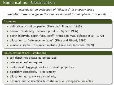
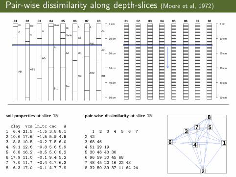
Pair-wise dissimilarity along depth-slices (Moore et al, 1972)

Oi

A

AB

01

Oe

A

AB1

02

A

AB

03Oi/A

A

Bt1

04

Oi

Oe/A

Ad

Bw

05

A

AB

Bt1

Bt2

06

A

AB1

AB2

07

A1

A2

Bt1

08

50 cm

40 cm

30 cm

20 cm

10 cm

0 cm

0

01 02 03 04 05 06 07 08

50 cm

40 cm

30 cm

20 cm

10 cm

0 cm

soil properties at slice 15

clay vcs ln_tc cec A1 6.4 21.5 -1.5 3.8 8.12 10.6 17.6 -1.5 5.9 4.93 8.8 10.5 -0.2 7.5 6.04 9.1 12.6 -0.8 5.6 5.95 6.8 16.2 -0.5 5.0 8.26 17.9 11.0 -0.1 9.4 5.27 7.0 11.7 -0.4 4.7 6.38 6.3 17.0 -0.1 4.7 7.9

pair-wise dissimilarity at slice 15

1 2 3 4 5 6 72 423 68 464 51 29 195 30 46 40 306 96 59 30 45 687 48 45 20 16 22 488 32 50 39 37 11 64 24

1

2

3

4

5

6

7

8

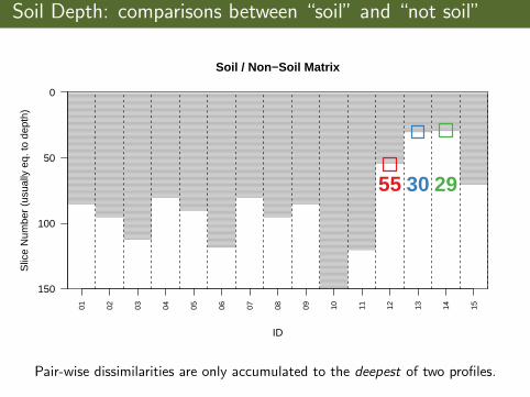
Soil Depth: comparisons between “soil” and “not soil”

Soil / Non−Soil Matrix

ID

Slic

e N

umbe

r (u

sual

ly e

q. to

dep

th)

150

100

50

001 02 03 04 05 06 07 08 09 10 11 12 13 14 15

55 30 29

Pair-wise dissimilarities are only accumulated to the deepest of two profiles.

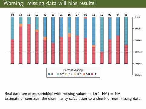
Warning: missing data will bias results!

08 14 13 12 09 03 01 15 07 05 11 10 02 04 06

250 cm

200 cm

150 cm

100 cm

50 cm

0 cm

Percent Missing

0 0.2 0.4 0.6 0.8 1

Real data are often sprinkled with missing values → D(6, NA) = NA.Estimate or constrain the dissimilarity calculation to a chunk of non-missing data.

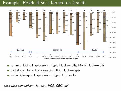
Example: Residual Soils formed on Granite

A1

A2

Bt1

Bt2

Cr

R

08A1

A2

A/C

CrR

14

A1

A2

R

13

A

Bw1

Bw2

Bw3

CrR

12

A

Bw1

Bw2

Crt

09

A

AB

Bt1

Bt2

Cr

03OiA

AB

Bt

Crt

01A1A2

Bw1

Bw2

Cr

15A

AB1

AB2

Bw1

Bw2R

07OiOe/A

Ad

Bw

Cr/Bw

Cr

05

A

AB1

AB2

Bt1

Bt2

Crt

11

A

AB

EC1

EC2

BC

10OeA

AB1

AB2

Bt

02Oi/A

A

Bt1

Bt2

04AAB

Bt1

Bt2

Bt3

BC

CB

R

06

180 cm

160 cm

140 cm

120 cm

100 cm

80 cm

60 cm

40 cm

20 cm

0 cm

Summit Backslope Swale

0.98 0.79 0.67 0.4 0.3 −0.05 −0.05 −0.09 −0.13 −0.3 −0.51 −0.54 −0.81 −0.86 −0.97Relative Topographic Position (50 meter radius)

summit: Lithic Haploxerolls, Typic Haploxerolls, Mollic Haploxeralfs

backslope: Typic Haploxerepts, Ultic Haploxerepts

swale: Oxyaquic Haploxerolls, Typic Argixerolls

slice-wise comparison via: clay, VCS, CEC, pH

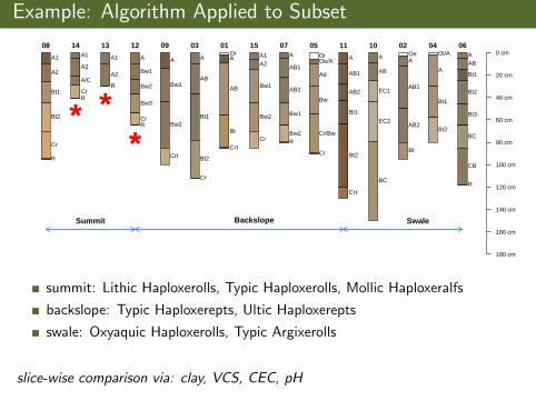
Example: Algorithm Applied to Subset

A1

A2

Bt1

Bt2

Cr

R

08A1

A2

A/C

CrR

14

A1

A2

R

13

A

Bw1

Bw2

Bw3

CrR

12

A

Bw1

Bw2

Crt

09

A

AB

Bt1

Bt2

Cr

03OiA

AB

Bt

Crt

01A1A2

Bw1

Bw2

Cr

15A

AB1

AB2

Bw1

Bw2R

07OiOe/A

Ad

Bw

Cr/Bw

Cr

05

A

AB1

AB2

Bt1

Bt2

Crt

11

A

AB

EC1

EC2

BC

10OeA

AB1

AB2

Bt

02Oi/A

A

Bt1

Bt2

04AAB

Bt1

Bt2

Bt3

BC

CB

R

06

180 cm

160 cm

140 cm

120 cm

100 cm

80 cm

60 cm

40 cm

20 cm

0 cm

* **






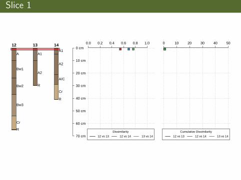
Slice 1

A

Bw1

Bw2

Bw3

Cr

R

12

A1

A2

R

13A1

A2

A/C

Cr

R

14

70 cm

60 cm

50 cm

40 cm

30 cm

20 cm

10 cm

0 cm

Dep

th

0.0 0.2 0.4 0.6 0.8 1.0

Dissimilarity

12 vs 13 12 vs 14 13 vs 14

Dep

th

0 10 20 30 40 50

Cumulative Dissimilarity

12 vs 13 12 vs 14 13 vs 14

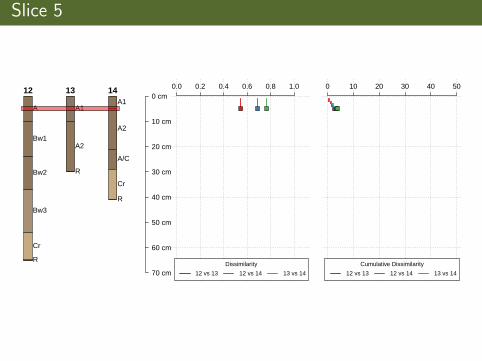
Slice 5

A

Bw1

Bw2

Bw3

Cr

R

12

A1

A2

R

13A1

A2

A/C

Cr

R

14

70 cm

60 cm

50 cm

40 cm

30 cm

20 cm

10 cm

0 cm

Dep

th

0.0 0.2 0.4 0.6 0.8 1.0

Dissimilarity

12 vs 13 12 vs 14 13 vs 14

Dep

th

0 10 20 30 40 50


12 vs 13 12 vs 14 13 vs 14

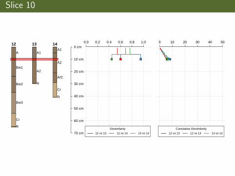
Slice 10

A

Bw1

Bw2

Bw3

Cr

R

12

A1

A2

R

13A1

A2

A/C

Cr

R

14

70 cm

60 cm

50 cm

40 cm

30 cm

20 cm

10 cm

0 cm

Dep

th

0.0 0.2 0.4 0.6 0.8 1.0

Dissimilarity

12 vs 13 12 vs 14 13 vs 14

Dep

th

0 10 20 30 40 50


12 vs 13 12 vs 14 13 vs 14

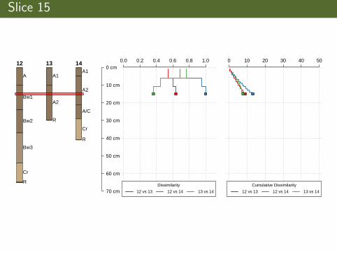
Slice 15

A

Bw1

Bw2

Bw3

Cr

R

12

A1

A2

R

13A1

A2

A/C

Cr

R

14

70 cm

60 cm

50 cm

40 cm

30 cm

20 cm

10 cm

0 cm

Dep

th

0.0 0.2 0.4 0.6 0.8 1.0

Dissimilarity

12 vs 13 12 vs 14 13 vs 14

Dep

th

0 10 20 30 40 50


12 vs 13 12 vs 14 13 vs 14

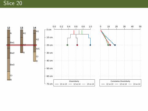
Slice 20

A

Bw1

Bw2

Bw3

Cr

R

12

A1

A2

R

13A1

A2

A/C

Cr

R

14

70 cm

60 cm

50 cm

40 cm

30 cm

20 cm

10 cm

0 cm

Dep

th

0.0 0.2 0.4 0.6 0.8 1.0

Dissimilarity

12 vs 13 12 vs 14 13 vs 14

Dep

th

0 10 20 30 40 50


12 vs 13 12 vs 14 13 vs 14

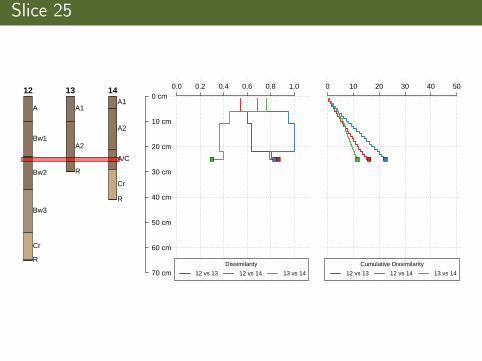
Slice 25

A

Bw1

Bw2

Bw3

Cr

R

12

A1

A2

R

13A1

A2

A/C

Cr

R

14

70 cm

60 cm

50 cm

40 cm

30 cm

20 cm

10 cm

0 cm

Dep

th

0.0 0.2 0.4 0.6 0.8 1.0

Dissimilarity

12 vs 13 12 vs 14 13 vs 14

Dep

th

0 10 20 30 40 50


12 vs 13 12 vs 14 13 vs 14

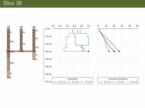
Slice 30

A

Bw1

Bw2

Bw3

Cr

R

12

A1

A2

R

13A1

A2

A/C

Cr

R

14

70 cm

60 cm

50 cm

40 cm

30 cm

20 cm

10 cm

0 cm

Dep

th

0.0 0.2 0.4 0.6 0.8 1.0

Dissimilarity

12 vs 13 12 vs 14 13 vs 14

Dep

th

0 10 20 30 40 50


12 vs 13 12 vs 14 13 vs 14

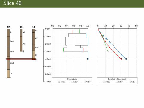
Slice 40

A

Bw1

Bw2

Bw3

Cr

R

12

A1

A2

R

13A1

A2

A/C

Cr

R

14

70 cm

60 cm

50 cm

40 cm

30 cm

20 cm

10 cm

0 cm

Dep

th

0.0 0.2 0.4 0.6 0.8 1.0

Dissimilarity

12 vs 13 12 vs 14 13 vs 14

Dep

th

0 10 20 30 40 50


12 vs 13 12 vs 14 13 vs 14

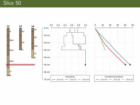
Slice 50

A

Bw1

Bw2

Bw3

Cr

R

12

A1

A2

R

13A1

A2

A/C

Cr

R

14

70 cm

60 cm

50 cm

40 cm

30 cm

20 cm

10 cm

0 cm

Dep

th

0.0 0.2 0.4 0.6 0.8 1.0

Dissimilarity

12 vs 13 12 vs 14 13 vs 14

Dep

th

0 10 20 30 40 50


12 vs 13 12 vs 14 13 vs 14

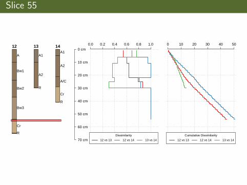
Slice 55

A

Bw1

Bw2

Bw3

Cr

R

12

A1

A2

R

13A1

A2

A/C

Cr

R

14

70 cm

60 cm

50 cm

40 cm

30 cm

20 cm

10 cm

0 cm

Dep

th

0.0 0.2 0.4 0.6 0.8 1.0

Dissimilarity

12 vs 13 12 vs 14 13 vs 14

Dep

th

0 10 20 30 40 50


12 vs 13 12 vs 14 13 vs 14

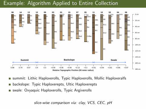
Example: Algorithm Applied to Entire Collection

A1

A2

Bt1

Bt2

Cr

R

08A1

A2

A/C

CrR

14

A1

A2

R

13

A

Bw1

Bw2

Bw3

CrR

12

A

Bw1

Bw2

Crt

09

A

AB

Bt1

Bt2

Cr

03OiA

AB

Bt

Crt

01A1A2

Bw1

Bw2

Cr

15A

AB1

AB2

Bw1

Bw2R

07OiOe/A

Ad

Bw

Cr/Bw

Cr

05

A

AB1

AB2

Bt1

Bt2

Crt

11

A

AB

EC1

EC2

BC

10OeA

AB1

AB2

Bt

02Oi/A

A

Bt1

Bt2

04AAB

Bt1

Bt2

Bt3

BC

CB

R

06

180 cm

160 cm

140 cm

120 cm

100 cm

80 cm

60 cm

40 cm

20 cm

0 cm


0.98 0.79 0.67 0.4 0.3 −0.05 −0.05 −0.09 −0.13 −0.3 −0.51 −0.54 −0.81 −0.86 −0.97Relative Topographic Position (50 meter radius)





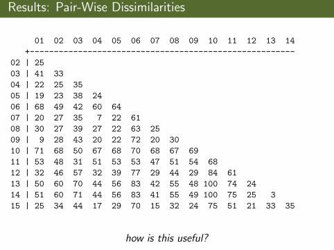
Results: Pair-Wise Dissimilarities

01 02 03 04 05 06 07 08 09 10 11 12 13 14

+-------------------------------------------------------

02 | 25

03 | 41 33

04 | 22 25 35

05 | 19 23 38 24

06 | 68 49 42 60 64

07 | 20 27 35 7 22 61

08 | 30 27 39 27 22 63 25

09 | 9 28 43 20 22 72 20 30

10 | 71 68 50 67 68 70 68 67 69

11 | 53 48 31 51 53 53 47 51 54 68

12 | 32 46 57 32 39 77 29 44 29 84 61

13 | 50 60 70 44 56 83 42 55 48 100 74 24

14 | 51 60 71 44 56 83 41 55 49 100 75 25 3

15 | 25 34 44 17 29 70 15 32 24 75 51 21 33 35

how is this useful?

Results: Dendrogram Representation

0

10

20

30

40

50

60

70

Oi/A

A

Bt1

Bt2

04A

AB1

AB2

Bw1

Bw2R

07

A1A2

Bw1

Bw2

Cr

15OiA

AB

Bt

Crt

01

A

Bw1

Bw2

Crt

09

OiOe/A

Ad

Bw

Cr/Bw

Cr

05

A1

A2

Bt1

Bt2

Cr

R

08OeA

AB1

AB2

Bt

02

A1

A2

R

13A1

A2

A/C

CrR

14

A

Bw1

Bw2

Bw3

CrR

12

A

AB

Bt1

Bt2

Cr

03

A

AB1

AB2

Bt1

Bt2

Crt

11AAB

Bt1

Bt2

Bt3

BC

CB

R

06

A

AB

EC1

EC2

BC

10

160 cm

140 cm

120 cm

100 cm

80 cm

60 cm

40 cm

20 cm

0 cm

Group 1Group 2Group 3Group 4

divisive, hierarchical clustering

what does it mean?

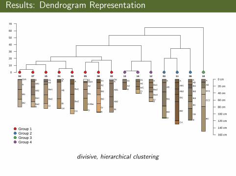
Results: Dendrogram Representation

0

10

20

30

40

50

60

70

Oi/A

A

Bt1

Bt2

04A

AB1

AB2

Bw1

Bw2R

07

A1A2

Bw1

Bw2

Cr

15OiA

AB

Bt

Crt

01

A

Bw1

Bw2

Crt

09

OiOe/A

Ad

Bw

Cr/Bw

Cr

05

A1

A2

Bt1

Bt2

Cr

R

08OeA

AB1

AB2

Bt

02

A1

A2

R

13A1

A2

A/C

CrR

14

A

Bw1

Bw2

Bw3

CrR

12

A

AB

Bt1

Bt2

Cr

03

A

AB1

AB2

Bt1

Bt2

Crt

11AAB

Bt1

Bt2

Bt3

BC

CB

R

06

A

AB

EC1

EC2

BC

10

160 cm

140 cm

120 cm

100 cm

80 cm

60 cm

40 cm

20 cm

0 cm

Group 1Group 2Group 3Group 4

divisive, hierarchical clustering

what does it mean?

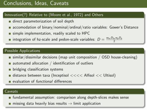
Conclusions, Ideas, Caveats

Innovation(?) Relative to (Moore et al., 1972) and Others

direct parameterization of soil depth

accomodation of binary/nominal/ordinal/ratio variables: Gower’s Distance

simple implementation, readily scaled to HPC

integration of hz-scale and pedon-scale variables: D =whzDhzwpDp

2

Possible Applications

similar/dissimilar decisions (map unit composition / OSD house-cleaning)

automated allocation / identification of outliers

bridging classification systems

distance between taxa (Inceptisol <<<< Alfisol << Ultisol)

evaluation of functional differences

Caveats

fundamental assumption: comparison along depth-slices makes sense

missing data heavily bias results → limit application

Thank You

Algorithms for Quantitative Pedology:http://aqp.r-forge.r-project.org

http://aqp.r-forge.r-project.org

Documents

A generalized algorithm for determining pair-wise ...ncss-tech.github.io/AQP/presentations/AQP-num_soil_classification.pdf · A generalized algorithm for determining pair-wise dissimilarity