Embed Size (px)
Citation preview
A General Valuation Framework for SABR andStochastic Local Volatility Models
Zhenyu Cui 1 J. Lars Kirkby 2 Duy Nguyen3
Mathematical Finance, Probability, and Partial Di↵erentialEquations Conference
Rutgers, The State University of New Jersey
May 19th, 2017
1School of Business, Stevens Institute of Technology, Hoboken, NJ 07310.Email: [email protected]
2School of Industrial and Systems Engineering, Georgia Institute ofTechnology, Atlanta, GA 30318, Email: [email protected]
3Department of Mathematics, Marist College, Poughkeepsie, NY 12601,Email:[email protected]
Overview
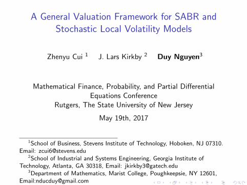
I Stochastic local volatility (SLV) models, including:I SABR (variants: shifted, lambda, Heston, etc.)I Quadratic SLV (Lipton), root quadratic SLV
I Includes pure stochastic volatility (SV) as special case:I Heston, Jacobi, Hull-White, 3/2, Stein-Stein, 4/2, Scott,
↵-Hypergeometric, etc.
I Includes mean-reverting Commodity models:I Ornstein-Uhlenbeck with SV, mean-reverting SABR, etc.
I Contracts: European, Bermudan/American, Barrier, Asian,Parisian/Occupation time, Lookback
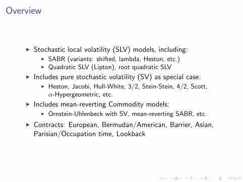
Stochastic Local Volatility
I Local volatility (Dupire (1994)4, Derman et al (1996)5), for“perfect calibration”:
LV : dSt
= St
µdt + �LV
(St
, t)St
dWt
I Stochastic volatility for realistic surface dynamics:
SV :
(dS
t
= St
µdt +m(vt
)St
dW(1)
t
,
dvt
= µ(vt
)dt + �(vt
)dW (2)
t
I Stochastic local volatility to unite the two:
SLV :
(dS
t
= !(St
, vt
)dt +m(vt
)�(St
)dW (1)
t
,
dvt
= µ(vt
)dt + �(vt
)dW (2)
t
4Dupire, B. (1994). Pricing with a Smile. Risk Magazine.5Derman, E., Kani, I., and Chriss, N. (1996). Implied trinomial tress of the
volatility smile. The Journal of Derivatives, 3(4), 7-22.
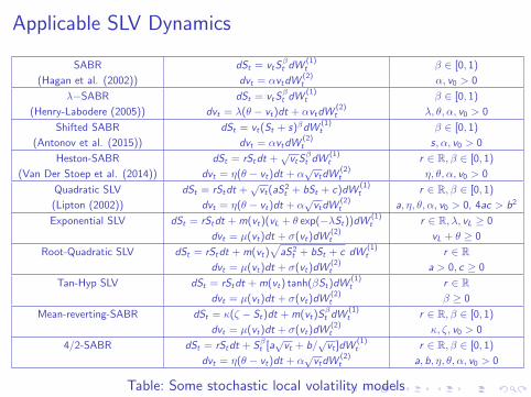
Applicable SLV Dynamics
SABR dSt
= vt
S�t
dW(1)
t
� 2 [0, 1)
(Hagan et al. (2002)) dvt
= ↵vt
dW(2)
t
↵, v0
> 0
��SABR dSt
= vt
S�t
dW(1)
t
� 2 [0, 1)
(Henry-Labodere (2005)) dvt
= �(✓ � vt
)dt + ↵vt
dW(2)
t
�, ✓,↵, v0
> 0
Shifted SABR dSt
= vt
(St
+ s)�dW (1)
t
� 2 [0, 1)
(Antonov et al. (2015)) dvt
= ↵vt
dW(2)
t
s,↵, v0
> 0
Heston-SABR dSt
= rSt
dt +pvt
S�t
dW(1)
t
r 2 R,� 2 [0, 1)
(Van Der Stoep et al. (2014)) dvt
= ⌘(✓ � vt
)dt + ↵pvt
dW(2)
t
⌘, ✓,↵, v0
> 0
Quadratic SLV dSt
= rSt
dt +pvt
(aS2
t
+ bSt
+ c)dW (1)
t
r 2 R,� 2 [0, 1)
(Lipton (2002)) dvt
= ⌘(✓ � vt
)dt + ↵pvt
dW(2)
t
a, ⌘, ✓,↵, v0
> 0, 4ac > b2
Exponential SLV dSt
= rSt
dt +m(vt
)(vL
+ ✓ exp(��St
))dW (1)
t
r 2 R,�, vL
� 0
dvt
= µ(vt
)dt + �(vt
)dW (2)
t
vL
+ ✓ � 0
Root-Quadratic SLV dSt
= rSt
dt +m(vt
)p
aS2
t
+ bSt
+ c dW(1)
t
r 2 Rdv
t
= µ(vt
)dt + �(vt
)dW (2)
t
a > 0, c � 0
Tan-Hyp SLV dSt
= rSt
dt +m(vt
) tanh(�St
)dW (1)
t
r 2 Rdv
t
= µ(vt
)dt + �(vt
)dW (2)
t
� � 0
Mean-reverting-SABR dSt
= (⇣ � St
)dt +m(vt
)S�t
dW(1)
t
r 2 R,� 2 [0, 1)
dvt
= µ(vt
)dt + �(vt
)dW (2)
t
, ⇣, v0
> 0
4/2-SABR dSt
= rSt
dt + S�t
[apvt
+ b/pvt
]dW (1)
t
r 2 R,� 2 [0, 1)
dvt
= ⌘(✓ � vt
)dt + ↵pvt
dW(2)
t
a, b, ⌘, ✓,↵, v0
> 0
Table: Some stochastic local volatility models
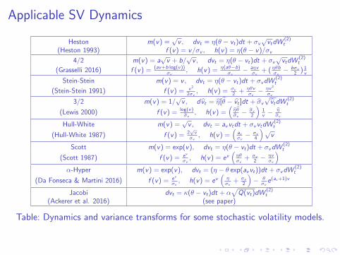
Applicable SV Dynamics
Heston m(v) =pv , dv
t
= ⌘(✓ � vt
)dt + �v
pvt
dW(2)
t
(Heston 1993) f (v) = v/�v
, h(v) = ⌘(✓ � v)/�v
4/2 m(v) = apv + b/
pv , dv
t
= ⌘(✓ � vt
)dt + �v
pvt
dW(2)
t
(Grasselli 2016) f (v) = (av+b log(v))
�v
, h(v) = ⌘(a✓�b)
�v
� a⌘v�v
+ (⌘✓b�v
� b�v
2
) 1v
Stein-Stein m(v) = v , dvt
= ⌘(✓ � vt
)dt + �v
dW(2)
t
(Stein-Stein 1991) f (v) = v
2
2�v
, h(v) = �v
2
+ ⌘✓v�v
� ⌘v2
�v
3/2 m(v) = 1/pv , dbv
t
= b⌘[b✓ � bvt
]dt + b�v
pbvt
dW(2)
t
(Lewis 2000) f (v) = log(v)
b�v
, h(v) =⇣
b⌘b✓b�v
� b�v
2
⌘1
v
� b⌘b�v
Hull-White m(v) =pv , dv
t
= av
vt
dt + �v
vt
dW(2)
t
(Hull-White 1987) f (v) = 2
pv
�v
, h(v) =⇣
a
v
�v
� �v
4
⌘pv
Scott m(v) = exp(v), dvt
= ⌘(✓ � vt
)dt + �v
dW(2)
t
(Scott 1987) f (v) = e
v
�v
, h(v) = ev⇣
⌘✓�v
+ �v
2
� ⌘v�v
⌘
↵-Hyper m(v) = exp(v), dvt
= (⌘ � ✓ exp(av
vt
))dt + �v
dW(2)
t
(Da Fonseca & Martini 2016) f (v) = e
v
�v
, h(v) = ev⇣
⌘�v
+ �v
2
⌘� ✓
�v
e(av+1)v
Jacobi dvt
= (✓ � vt
)dt + ↵p
Q(vt
)dW (2)
t
(Ackerer et al. 2016) (see paper)
Table: Dynamics and variance transforms for some stochastic volatility models.
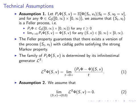
Technical AssumptionsI Assumption 1. Let P
t
�(S , v) = E[�(St
, vt
)|S0
= S , v0
= v ],and for any � 2 C
0
([0,1)⇥ [0,1)), we assume that (St
, vt
)is a Feller process, i.e.
I Pt
� 2 C0
([0,1)⇥ [0,1)) for any t � 0I lim
t!0
Pt
�(S , v) = �(S , v) for any (S , v) 2 [0,1)⇥ [0,1).
I The Feller property guarantees that there exists a version ofthe process (S
t
, vt
) with cadlag paths satisfying the strongMarkov property.
I The family of Pt
�(S , v) is determined by its infinitestimalgenerator LS :
LS�(S , v) = limt!0+
(Pt
�� �)(S , v)t
. (1)
I Assumption 2. We assume that
lim(S ,v)!(0,0)
LS�(S , v) = 0. (2)
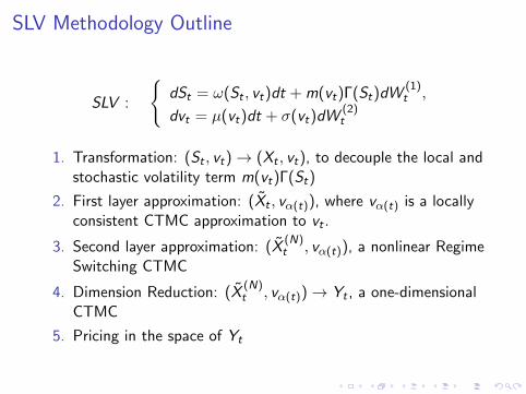
SLV Methodology Outline
SLV :
(dS
t
= !(St
, vt
)dt +m(vt
)�(St
)dW (1)
t
,
dvt
= µ(vt
)dt + �(vt
)dW (2)
t
1. Transformation: (St
, vt
) ! (Xt
, vt
), to decouple the local andstochastic volatility term m(v
t
)�(St
)
2. First layer approximation: (Xt
, v↵(t)), where v↵(t) is a locallyconsistent CTMC approximation to v
t
.
3. Second layer approximation: (X (N)
t
, v↵(t)), a nonlinear RegimeSwitching CTMC
4. Dimension Reduction: (X (N)
t
, v↵(t)) ! Yt
, a one-dimensionalCTMC
5. Pricing in the space of Yt
Transformed Process
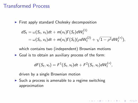
I First apply standard Cholesky decomposition
dSt
= !(St
, vt
)dt +m(vt
)�(St
)dW (1)
t
= !(St
, vt
)dt +m(vt
)�(St
)(⇢dW (2)
t
+p
1� ⇢2dW (⇤)t
),
which contains two (independent) Brownian motions
I Goal is to obtain an auxiliary process of the form:
dF (St
, vt
) = F 1(St
, vt
)dt + F 2(St
, vt
)dW (⇤)t
,
driven by a single Brownian motion
I Such a process is amenable to a regime switchingapproximation
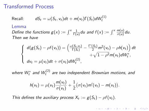
Transformed Process
Recall: dSt
= !(St
, vt
)dt +m(vt
)�(St
)dW (1)
t
LemmaDefine the functions g(x) :=
Rx
·1
�(u)
du and f (x) :=Rx
·m(u)
�(u) du.Then we have
8><
>:
d(g(St
)� ⇢f (vt
)) =⇣!(S
t
,vt
)
�(S
t
)
� �
0(S
t
)
2
m2(vt
)� ⇢h(vt
)⌘dt
+p
1� ⇢2m(vt
)dW ⇤t
,
dvt
= µ(vt
)dt + �(vt
)dW (2)
t
,
where W ⇤t
and W(2)
t
are two independent Brownian motions, and
h(vt
) = µ(vt
)m(v
t
)
�(vt
)+
1
2
��(v
t
)m0(vt
)�m(vt
)�.
This defines the auxiliary process Xt
:= g(St
)� ⇢f (vt
).
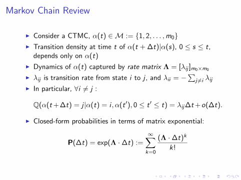
Markov Chain Review
I Consider a CTMC, ↵(t) 2 M := {1, 2, . . . ,m0
}I Transition density at time t of ↵(t +�t)|↵(s), 0 s t,
depends only on ↵(t)
I Dynamics of ↵(t) captured by rate matrix ⇤ = [�ij
]m
0
⇥m
0
I �ij
is transition rate from state i to j , and �ii
= �P
j 6=i
�ij
I In particular, 8i 6= j :
Q(↵(t+�t) = j |↵(t) = i ,↵(t 0), 0 t 0 t) = �ij
�t+o(�t).
I Closed-form probabilities in terms of matrix exponential:
P(�t) = exp(⇤ ·�t) :=1X
k=0
(⇤ ·�t)k
k!
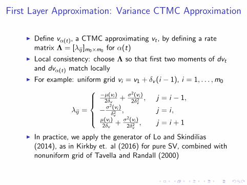
First Layer Approximation: Variance CTMC Approximation
I Define v↵(t), a CTMC approximating vt
, by defining a ratematrix ⇤ = [�
ij
]m
0
⇥m
0
for ↵(t)
I Local consistency: choose ⇤ so that first two moments of dvt
and dv↵(t) match locally
I For example: uniform grid vi
= v1
+ �v
(i � 1), i = 1, . . . ,m0
�ij
=
8>><
>>:
�µ(vi
)
2�v
+ �2
(v
i
)
2�2v
, j = i � 1,
��2
(v
i
)
�2v
, j = i ,µ(v
i
)
2�v
+ �2
(v
i
)
2�2v
, j = i + 1
I In practice, we apply the generator of Lo and Skindilias(2014), as in Kirkby et. al (2016) for pure SV, combined withnonuniform grid of Tavella and Randall (2000)
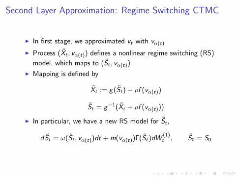
Second Layer Approximation: Regime Switching CTMC
I In first stage, we approximated vt
with v↵(t)
I Process (Xt
, v↵(t)) defines a nonlinear regime switching (RS)
model, which maps to (St
, v↵(t))
I Mapping is defined by
Xt
:= g(St
)� ⇢f (v↵(t))
St
= g�1(Xt
+ ⇢f (v↵(t)))
I In particular, we have a new RS model for St
,
dSt
= !(St
, v↵(t))dt +m(v↵(t))�(St)dW(1)
t
, S0
= S0
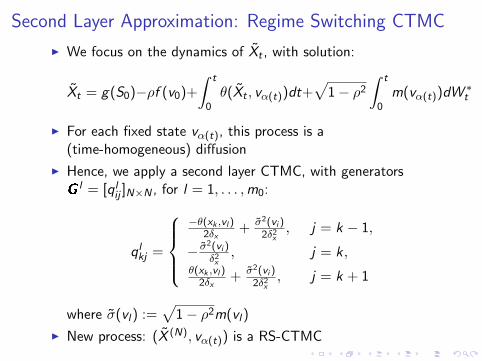
Second Layer Approximation: Regime Switching CTMC
I We focus on the dynamics of Xt
, with solution:
Xt
= g(S0
)�⇢f (v0
)+
Zt
0
✓(Xt
, v↵(t))dt+p1� ⇢2
Zt
0
m(v↵(t))dW⇤t
I For each fixed state v↵(t), this process is a(time-homogeneous) di↵usion
I Hence, we apply a second layer CTMC, with generatorsl = [ql
ij
]N⇥N
, for l = 1, . . . ,m0
:
qlkj
=
8>><
>>:
�✓(xk
,vl
)
2�x
+ �2
(v
i
)
2�2x
, j = k � 1,
� �2
(v
i
)
�2x
, j = k ,✓(x
k
,vl
)
2�x
+ �2
(v
i
)
2�2x
, j = k + 1
where �(vl
) :=p
1� ⇢2m(vl
)
I New process: (X (N), v↵(t)) is a RS-CTMC
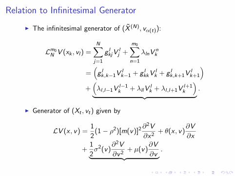
Relation to Infinitesimal Generator
I The infinitesimal generator of (X (N), v↵(t)):
Lm
0
N
V (xk
, vl
) =NX
j=1
g l
kj
V l
j
+m
0X
n=1
�ln
V n
k
=⇣g l
k,k�1
V l
k�1
+ g l
kk
V l
k
+ g l
k,k+1
V l
k+1
⌘
+⇣�l ,l�1
V l�1
k
+ �ll
V l
k
+ �l ,l+1
V l+1
k
⌘
| {z }.
I Generator of (Xt
, vt
) given by
LV (x , v) =1
2(1� ⇢2)[m(v)]2
@2V
@x2+ ✓(x , v)
@V
@x
+1
2�2(v)
@2V
@v2+ µ(v)
@V
@v| {z }.
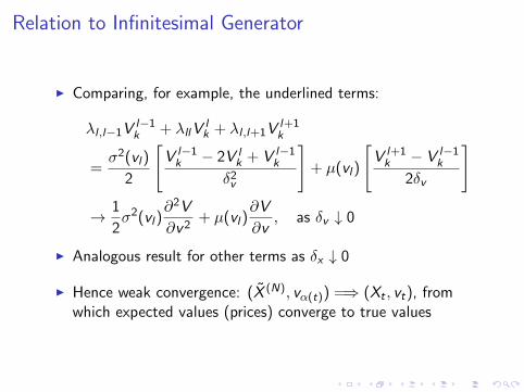
Relation to Infinitesimal Generator
I Comparing, for example, the underlined terms:
�l ,l�1
V l�1
k
+ �ll
V l
k
+ �l ,l+1
V l+1
k
=�2(v
l
)
2
"V l�1
k
� 2V l
k
+ V l�1
k
�2v
#+ µ(v
l
)
"V l+1
k
� V l�1
k
2�v
#
! 1
2�2(v
l
)@2V
@v2+ µ(v
l
)@V
@v, as �
v
# 0
I Analogous result for other terms as �x
# 0
I Hence weak convergence: (X (N), v↵(t)) =) (Xt
, vt
), fromwhich expected values (prices) converge to true values
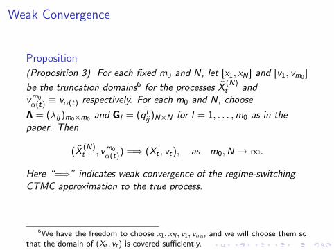
Weak Convergence
Proposition(Proposition 3) For each fixed m
0
and N, let [x1
, xN
] and [v1
, vm
0
]
be the truncation domains6 for the processes X(N)
t
andvm0
↵(t) ⌘ v↵(t) respectively. For each m0
and N, choose
⇤ = (�ij
)m
0
⇥m
0
and Gl
= (qlij
)N⇥N
for l = 1, . . . ,m0
as in thepaper. Then
(X (N)
t
, vm0
↵(t)) =) (Xt
, vt
), as m0
,N ! 1.
Here “=)” indicates weak convergence of the regime-switchingCTMC approximation to the true process.
6We have the freedom to choose x
1
, xN
, v1
, vm
0
, and we will choose them sothat the domain of (X
t
, vt
) is covered su�ciently.
Convergence Order
I Li and Zhang (2016)7 consider an error estimate of the optionvalue using the Markov chain approximation of Mijatovic andPistorius (2013)8.
I Using the spectral analysis, they show that for call/put-typepayo↵s, the convergence is of second order, while fordigital-type payo↵s, the convergence is only of first order ingeneral.
I It is expected that the same convergence type would hold forthe model considered in this paper. It would be veryinteresting to carry this out. We leave this as an interestingproject for future studies.
7Li, L. and Zhang, G., 2016. Option Pricing in Some Non-Levy JumpModels. SIAM Journal on Scientific Computing, 38(4), pp.B539-B569.
8Mijatovic, A. and Pistorius, M., 2013. Continuously monitored barrieroptions under Markov processes. Mathematical Finance, 23(1), pp.1-38.
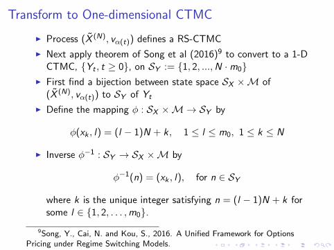
Transform to One-dimensional CTMC
I Process (X (N), v↵(t)) defines a RS-CTMC
I Next apply theorem of Song et al (2016)9 to convert to a 1-DCTMC, {Y
t
, t � 0}, on SY
:= {1, 2, ...,N ·m0
}I First find a bijection between state space S
X
⇥M of(X (N), v↵(t)) to S
Y
of Yt
I Define the mapping � : SX
⇥M ! SY
by
�(xk
, l) = (l � 1)N + k , 1 l m0
, 1 k N
I Inverse ��1 : SY
! SX
⇥M by
��1(n) = (xk
, l), for n 2 SY
where k is the unique integer satisfying n = (l � 1)N + k forsome l 2 {1, 2, . . . ,m
0
}.9Song, Y., Cai, N. and Kou, S., 2016. A Unified Framework for Options
Pricing under Regime Switching Models.
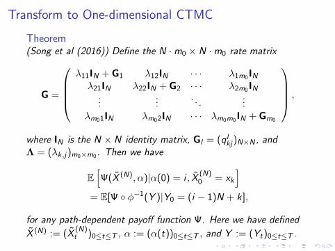
Transform to One-dimensional CTMC
Theorem(Song et al (2016)) Define the N ·m
0
⇥ N ·m0
rate matrix
G =
0
BBB@
�11
IN
+ G1
�12
IN
· · · �1m
0
IN
�21
IN
�22
IN
+ G2
· · · �2m
0
IN
......
. . ....
�m
0
1
IN
�m
0
2
IN
· · · �m
0
m
0
IN
+ Gm
0
1
CCCA,
where IN
is the N ⇥ N identity matrix, Gl
= (qlkj
)N⇥N
, and⇤ = (�
k,j)m0
⇥m
0
. Then we have
Eh (X (N),↵)|↵(0) = i , X (N)
0
= xk
i
= E[ � ��1(Y )|Y0
= (i � 1)N + k],
for any path-dependent payo↵ function . Here we have defined
X (N) := (X (N)
t
)0tT
, ↵ := (↵(t))0tT
, and Y := (Yt
)0tT
.
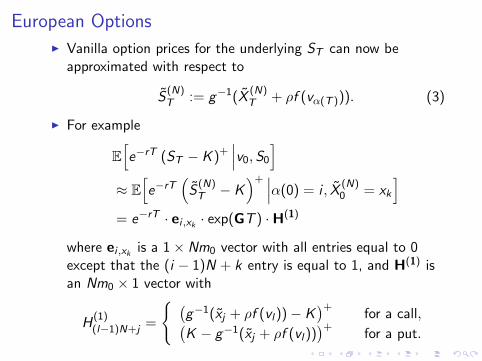
European OptionsI Vanilla option prices for the underlying S
T
can now beapproximated with respect to
S(N)
T
:= g�1(X (N)
T
+ ⇢f (v↵(T )
)). (3)
I For example
Ehe�rT (S
T
� K )+���v
0
, S0
i
⇡ Ehe�rT
⇣S(N)
T
� K⌘+
���↵(0) = i , X (N)
0
= xk
i
= e�rT · ei ,x
k
· exp(GT ) ·H(1)
where ei ,x
k
is a 1⇥ Nm0
vector with all entries equal to 0except that the (i � 1)N + k entry is equal to 1, and H(1) isan Nm
0
⇥ 1 vector with
H(1)
(l�1)N+j
=
( �g�1(x
j
+ ⇢f (vl
))� K�+
for a call,�K � g�1(x
j
+ ⇢f (vl
))�+
for a put.
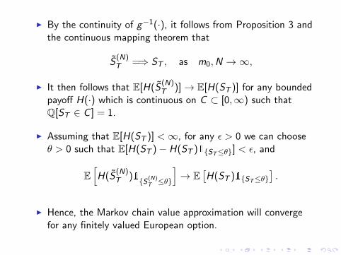
I By the continuity of g�1(·), it follows from Proposition 3 andthe continuous mapping theorem that
S(N)
T
=) ST
, as m0
,N ! 1,
I It then follows that E[H(S (N)
T
)] ! E[H(ST
)] for any boundedpayo↵ H(·) which is continuous on C ⇢ [0,1) such thatQ[S
T
2 C ] = 1.
I Assuming that E[H(ST
)] < 1, for any ✏ > 0 we can choose✓ > 0 such that E[H(S
T
)� H(ST
) {ST
✓}] < ✏, and
EhH(S (N)
T
) {S(N)
T
✓}
i! E
⇥H(S
T
) {ST
✓}⇤.
I Hence, the Markov chain value approximation will convergefor any finitely valued European option.
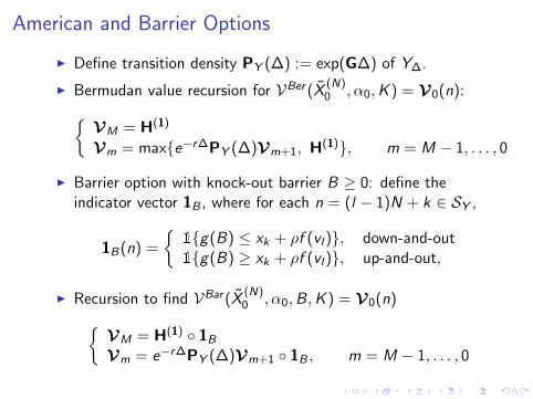
American and Barrier Options
I Define transition density PY
(�) := exp(G�) of Y�
.
I Bermudan value recursion for VBer (X (N)
0
,↵0
,K ) = V0
(n):
⇢V
M
= H(1)
Vm
= max{e�r�PY
(�)Vm+1
, H(1)}, m = M � 1, . . . , 0
I Barrier option with knock-out barrier B � 0: define theindicator vector 1
B
, where for each n = (l � 1)N + k 2 SY
,
1B
(n) =
⇢{g(B) x
k
+ ⇢f (vl
)}, down-and-out{g(B) � x
k
+ ⇢f (vl
)}, up-and-out,
I Recursion to find VBar (X (N)
0
,↵0
,B ,K ) = V0
(n)
⇢V
M
= H(1) � 1B
Vm
= e�r�PY
(�)Vm+1
� 1B
, m = M � 1, . . . , 0
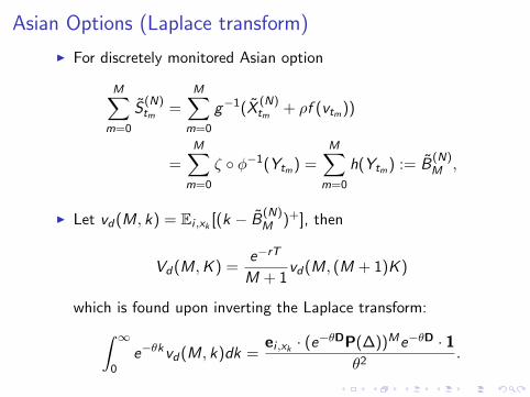
Asian Options (Laplace transform)
I For discretely monitored Asian option
MX
m=0
S(N)
t
m
=MX
m=0
g�1(X (N)
t
m
+ ⇢f (vt
m
))
=MX
m=0
⇣ � ��1(Yt
m
) =MX
m=0
h(Yt
m
) := B(N)
M
,
I Let vd
(M, k) = Ei ,x
k
[(k � B(N)
M
)+], then
Vd
(M,K ) =e�rT
M + 1vd
(M, (M + 1)K )
which is found upon inverting the Laplace transform:
Z 1
0
e�✓kvd
(M, k)dk =ei ,x
k
· (e�✓DP(�))Me�✓D · 1✓2
.
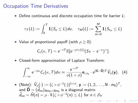
Occupation Time Derivatives
I Define continuous and discrete occupation time for barrier L:
⌧T
(L) :=
ZT
0
1{Su
L}du, ⌧M
(L) :=MX
m=0
1{St
m
L}
I Value of proportional payo↵ (with ⇢ � 0):
Cc
(,T ) = e�rTE[e�⇢⌧T
(L)(ST
� e�)+].
I Closed-form approximation of Laplace Transform:
Z 1
�1e��C
c
(,T )d ⇡ e�rT
�(1 + �)ei ,x
k
· e(G�D)T V�(y), (4)
I (Note): V�(·) := (⇣ � ��1(·))1+�, y := (1, 2, . . . ,N ·m0
)T ,and D = (d
nn
)Nm
0
⇥Nm
0
is a diagonal matrixdnn
= H(n) = ⇢ · {⇣ � ��1(n) L} for n 2 SY
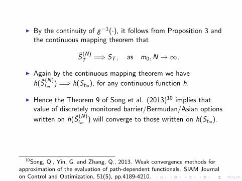
I By the continuity of g�1(·), it follows from Proposition 3 andthe continuous mapping theorem that
S(N)
T
=) ST
, as m0
,N ! 1,
I Again by the continuous mapping theorem we have
h(S (N)
t
m
) =) h(St
m
), for any continuous function h.
I Hence the Theorem 9 of Song et al. (2013)10 implies thatvalue of discretely monitored barrier/Bermudan/Asian options
written on h(S (N)
t
m
) will converge to those written on h(St
m
).
10Song, Q., Yin, G. and Zhang, Q., 2013. Weak convergence methods forapproximation of the evaluation of path-dependent functionals. SIAM Journalon Control and Optimization, 51(5), pp.4189-4210.
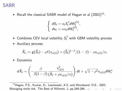
SABR
I Recall the classical SABR model of Hagan et al (2002)11:
(dS
t
= vt
S�t
dW(1)
t
,
dvt
= ↵vt
dW(2)
t
,
I Combines CEV local volatility S�t
with GBM volatility process
I Auxiliary process:
Xt
:= g(St
)� ⇢f (v↵(t)) = (St
)1��/(1� �)� ⇢v↵(t)/↵,
I Dynamics
dXt
=
� �
2(1� �)
v2↵(t)
(Xt
+ ⇢v↵(t)/↵)
!dt +
p1� ⇢2v↵(t)dW
⇤t
11Hagan, P.S., Kumar, D., Lesniewski, A.S. and Woodward, D.E., 2002.Managing smile risk. The Best of Wilmott, 1, pp.249-296.
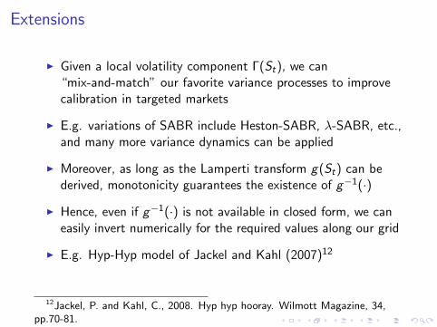
Extensions
I Given a local volatility component �(St
), we can“mix-and-match” our favorite variance processes to improvecalibration in targeted markets
I E.g. variations of SABR include Heston-SABR, �-SABR, etc.,and many more variance dynamics can be applied
I Moreover, as long as the Lamperti transform g(St
) can bederived, monotonicity guarantees the existence of g�1(·)
I Hence, even if g�1(·) is not available in closed form, we caneasily invert numerically for the required values along our grid
I E.g. Hyp-Hyp model of Jackel and Kahl (2007)12
12Jackel, P. and Kahl, C., 2008. Hyp hyp hooray. Wilmott Magazine, 34,pp.70-81.
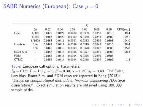
SABR Numerics (European): Case ⇢ = 0
K�t 0.02 0.04 0.05 0.06 0.08 0.10 CPU(sec.)
Euler 1/400 0.0472 0.0429 0.0409 0.0389 0.0352 0.0318 49.41/800 0.0463 0.0420 0.0399 0.0380 0.0343 0.0309 99.11/1600 0.0453 0.0411 0.0391 0.0372 0.0336 0.0303 194.0
Low-bias 1/4 0.0461 0.0419 0.0399 0.0379 0.0343 0.0310 78.41/8 0.0460 0.0418 0.0398 0.0378 0.0342 0.0308 175.8
Exact Sim - 0.0457 0.0416 0.0396 0.0377 0.0341 0.0308 98.3FDM - 0.0456 0.0414 0.0394 0.0375 0.0339 0.0306 -CTMC - 0.0456 0.0414 0.0394 0.0375 0.0339 0.0306 1.8
Table: European call options. Parameters:S0
= 0.05,T = 1.0, ⇢ = 0,� = 0.30,↵ = 0.60, v0
= 0.40. The Euler,Low-bias, Exact Sim, and FDM rows are reported in Song (2013):“Essays on computational methods in financial engineering (Doctoraldissertation)”. Exact simulation results are obtained using 100, 000sample paths.
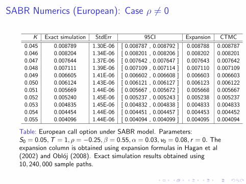
SABR Numerics (European): Case ⇢ 6= 0
K Exact simulation StdErr 95CI Expansion CTMC
0.045 0.008789 1.30E-06 [ 0.008787 , 0.008792 ] 0.008788 0.0087870.046 0.008204 1.34E-06 [ 0.008201 , 0.008206 ] 0.008202 0.0082010.047 0.007644 1.37E-06 [ 0.007642 , 0.007647 ] 0.007643 0.0076420.048 0.007111 1.39E-06 [ 0.007109 , 0.007114 ] 0.007110 0.0071090.049 0.006605 1.41E-06 [ 0.006602 , 0.006608 ] 0.006603 0.0066030.050 0.006124 1.43E-06 [ 0.006121 , 0.006127 ] 0.006123 0.0061220.051 0.005669 1.44E-06 [ 0.005667 , 0.005672 ] 0.005668 0.0056670.052 0.005240 1.45E-06 [ 0.005237 , 0.005243 ] 0.005238 0.0052370.053 0.004835 1.45E-06 [ 0.004832 , 0.004838 ] 0.004833 0.0048330.054 0.004454 1.44E-06 [ 0.004451 , 0.004457 ] 0.004453 0.0044520.055 0.004096 1.44E-06 [ 0.004094 , 0.004099 ] 0.004095 0.004094
Table: European call option under SABR model. Parameters:S0
= 0.05,T = 1, ⇢ = �0.25,� = 0.55,↵ = 0.03, v0
= 0.08, r = 0. Theexpansion column is obtained using expansion formulas in Hagan et al(2002) and Obloj (2008). Exact simulation results obtained using10, 240, 000 sample paths.
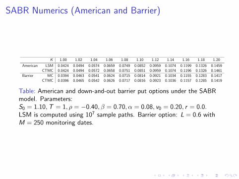
SABR Numerics (American and Barrier)
K 1.00 1.02 1.04 1.06 1.08 1.10 1.12 1.14 1.16 1.18 1.20
American LSM 0.0424 0.0494 0.0574 0.0659 0.0749 0.0852 0.0959 0.1074 0.1199 0.1326 0.1459CTMC 0.0424 0.0494 0.0572 0.0658 0.0751 0.0851 0.0959 0.1074 0.1196 0.1326 0.1461
Barrier MC 0.0394 0.0463 0.0541 0.0624 0.0715 0.0814 0.0921 0.1034 0.1155 0.1283 0.1417CTMC 0.0396 0.0465 0.0542 0.0626 0.0717 0.0816 0.0923 0.1036 0.1157 0.1285 0.1419
Table: American and down-and-out barrier put options under the SABRmodel. Parameters:S0
= 1.10,T = 1, ⇢ = �0.40,� = 0.70,↵ = 0.08, v0
= 0.20, r = 0.0.LSM is computed using 107 sample paths. Barrier option: L = 0.6 withM = 250 monitoring dates.
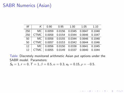
SABR Numerics (Asian)
M K 0.90 0.95 1.00 1.05 1.10
250 MC 0.0059 0.0156 0.0345 0.0647 0.1048250 CTMC 0.0058 0.0154 0.0344 0.0646 0.104750 MC 0.0058 0.0155 0.0344 0.0646 0.104850 CTMC 0.0057 0.0153 0.0342 0.0644 0.104612 MC 0.0056 0.0150 0.0338 0.0641 0.104512 CTMC 0.0055 0.0149 0.0337 0.0640 0.1044
Table: Discretely monitored arithmetic Asian put options under theSABR model. Parameters:S0
= 1, r = 0,T = 1,� = 0.5,↵ = 0.3, v0
= 0.15, ⇢ = �0.5.
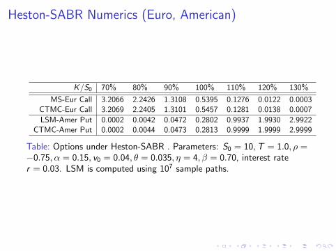
Heston-SABR Numerics (Euro, American)
K/S0
70% 80% 90% 100% 110% 120% 130%
MS-Eur Call 3.2066 2.2426 1.3108 0.5395 0.1276 0.0122 0.0003CTMC-Eur Call 3.2069 2.2405 1.3101 0.5457 0.1281 0.0138 0.0007LSM-Amer Put 0.0002 0.0042 0.0472 0.2802 0.9937 1.9930 2.9922
CTMC-Amer Put 0.0002 0.0044 0.0473 0.2813 0.9999 1.9999 2.9999
Table: Options under Heston-SABR . Parameters: S0
= 10,T = 1.0, ⇢ =�0.75,↵ = 0.15, v
0
= 0.04, ✓ = 0.035, ⌘ = 4,� = 0.70, interest rater = 0.03. LSM is computed using 107 sample paths.
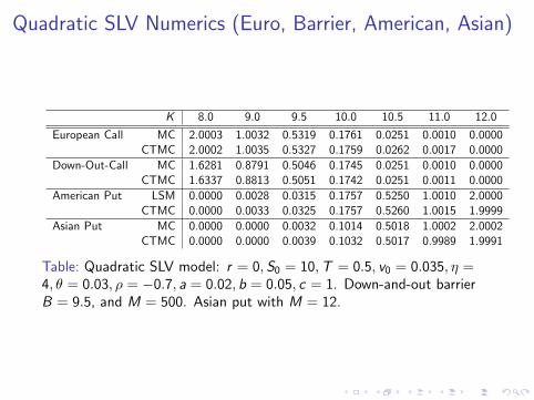
Quadratic SLV Numerics (Euro, Barrier, American, Asian)
K 8.0 9.0 9.5 10.0 10.5 11.0 12.0
European Call MC 2.0003 1.0032 0.5319 0.1761 0.0251 0.0010 0.0000CTMC 2.0002 1.0035 0.5327 0.1759 0.0262 0.0017 0.0000
Down-Out-Call MC 1.6281 0.8791 0.5046 0.1745 0.0251 0.0010 0.0000CTMC 1.6337 0.8813 0.5051 0.1742 0.0251 0.0011 0.0000
American Put LSM 0.0000 0.0028 0.0315 0.1757 0.5250 1.0010 2.0000CTMC 0.0000 0.0033 0.0325 0.1757 0.5260 1.0015 1.9999
Asian Put MC 0.0000 0.0000 0.0032 0.1014 0.5018 1.0002 2.0002CTMC 0.0000 0.0000 0.0039 0.1032 0.5017 0.9989 1.9991
Table: Quadratic SLV model: r = 0, S0
= 10,T = 0.5, v0
= 0.035, ⌘ =4, ✓ = 0.03, ⇢ = �0.7, a = 0.02, b = 0.05, c = 1. Down-and-out barrierB = 9.5, and M = 500. Asian put with M = 12.

Thank You
Q & A