Embed Size (px)
Citation preview

NASA Contractor Report 4496
A General Theory of Two- and
Three-Dimensional Rotational
Flow in Subsonic and
Transonic Turbomachines
Chung-Hua Wu
Clernson University
Clemson, South Carolina
Prepared for
Lewis Research Center
under Grant NAG3-1072
National Aeronautics and
Space Administration
Office of Management
Scientific and TechnicalInformation Program
1993
https://ntrs.nasa.gov/search.jsp?R=19950021582 2018-05-12T01:50:58+00:00Z

7|I

CONTENTS
FOREWORD ............................................................... v
SYMBOLS .................................. +............................... ix
CHAPTER 1--INTRODUCTION ............................... ................. 1
CHAPTER 2--FUNDAMENTAL AEROTHERMODYNAMIC EQUATIONS GOVERNING THETHREE-DIMENSIONAL FLOW IN TURBOMACHINES ........................... 6
2.1 Basic Aerothermodynamic Equations Governing the Three-Dimensional
Flow of a Viscous Fluid Through a Stationary Blade Row .............. .. ............ 6
2.2 Effect of Viscosity on Basic Equations ........................................... 9
2.3 Basic Aerothermodynamic Equations Governing the Three-Dimensional Flow of aViscous Fluid Through a Rotating Blade Row ................................... 21
2.4 Steady Fluid Flow Through a Stationary Blade Row andSteady Relative Flow Through a Rotating Blade Row ............................. 26
2.5 Viscous terms in the Governing Equations ....................................... 28
2.6 Some Remarks on the Energy Equation and the Entropy Equation ....... . ............. 31
CHAPTER 3--GOVERNING EQUATIONS FOR FLUID FLOW ALONG RELATIVE STREAMFILAMENTS .......................................................... 34
3.1 Following Fluid Flow on Relative Stream Surfaces ................................. 34
3.2 Equation Governing Fluid Flow Along S2 Stream Surfaceof S2 Stream Filament .......................................... ......... 36
3.3 Principal Equation for Fluid Flow Along S2 Stream Filament ........................ 41
3.4 Principal Equations for Fluid Flow Along S1 Stream Filament ....................... 50
CHAPTER 4--THREE-DIMENSIONAL FLOW EQUATIONS EXPRESSED IN TERMS OFNONORTHOGONAL CURVILINEAR COORDINATES AND CORRESPONDING
NONORTHOGONAL VELOCITY COMPONENTS ......... _ .................... 53
4.1 General Curvilinear Coordinates in a Three-Dimensional Space .... _........... . ..... . . . 53
4.2 General Curvilinear Coordinates on a Surface .................................... 57
4.3 Basic Equations Governing Fluid Flow on S 1 Surface of Revolution ................... . 60
4.4 Methods of Solution for S1 ................................................. 64
4.5 Equations Governing Fluid Flow on General S2 Surface ............................ 70
PAGI ,,fI, !mN NN W glIB
..q
lU
PREIMI)bNG PPlGE BLANK NOT FILMED

4.6 Governing Equations for S2 with Independent Variable ¢ Eliminated .................. 78
4.7 Methods of Solution For S_ Flow ............................................ 84
4.8 Computation of F Term in Inverse Problem .................................... 89
4.9 Computation of Components of Normal and W_ In Direct Problem ................... 90
CHAPTER 5--TWO- AND THREE-DIMENSIONAL SUBSONIC FLOWIN TURBOMACHINES ................................................... 92
5.1 Series Expansion on S1 Surface of Revolution ...................... , ............ 92
5.2 Series Expansion In _-coordinate .............................................. 96
5.3 Forming Successive S2 Surfaces by Progressing Circumferentially from $2, m 97
5.4 Coordinate Transformation and Direct Expansion Method ........................... 99
5.5 Direct Matrix Solution of Subsonic Flow Along S1 Filament of Revolution ............... 102
5.6 Three-Dimenslonal Subsonic Flow in Turbomachine ............................... 106
5.7 Three-Dimensional Flow in a High Subsonic Compressor Stator ....................... 111
5.8 Three-Dimensional Flow in CAS Research Compressor (Subsonic Case) .................. 113
CHAPTER 6--TRANSONIC FLOW ALONG S1 AND S2 STREAM FILAMENTS ......... 121
6.1 Transonic Flow Along S1 Stream Filament of Revolution Solved by SeparateRegion Computation with Shock Fitting ....................................... 121
6.2 Transonic Stream-Function Principal Equation Solved with the Use
of Artificial Compressibility ................................................ 124
6.3 Effect of Axlal-Velocity Density Ratio and Viscous Effect ............................ 129
6.4 Transonic Flow Along General S1 Stream Filament ............................... 131
6.5 Transonic Flow on S2 Stream Filament Solved by Separate Region Computation with ShockFitting ........................... 133
6.6 Shock Embedding Elliptic Solution for Inverse Problem of Transonic S2 Flow ............. 135
6.7 Direct-Problem Solution of Transonic Flow Along S2 Stream Filament ................. 138
CHAPTER 7--THREE-DIMENSIONAL FLOW IN TRANSONIC TURBOMACHINES ........ 142
7A Quasi-Three-Dimensional Flow Field in the DFVLR Rotor .......................... 142
7.2 Full-Three-Dimensional Transonic Flow in Cas Rotor .............................. 151
7.3 Some Remarks 164
References ................................................................. 166
iv
51li;
FOREWORD
Professor Chung-hua Wu pioneered the three-dimensional flow theory for turbomachines at Lewis
Flight Propulsion Laboratory, NACA in 1950. He introduced the S 1 and S2 families of relative stream
surfaces and thus reduced three-dimensional flow problems to problems of iterating two solutions of two
independent variables. The relaxation or direct matrix method was used for subsonic flows and the
method of characteristics for supersonic flows. Laborious but accurate results were obtained without the
benefit of modern digital computers. In the sixties Professor Wu developed a body-fitted, nonorthogonal
curvilinear coordinate system to improve computational accuracy. In subsequent years Professor Wu and
his colleagues at the Institute of Engineering Thermal Physics, the People's Republic of China, developed
shock-fitting and artificial compressibility methods for solutions in two- and three-dimensional transonic
flows. Professor Wu's theories were design tools used in aircraft engines such as the J69, JT-3D, Spe_,
RB211, JTgD, F404, etc.
Since the early sixties Clemson University has been active in internal flow analysis. Through the
support of the NASA Lewis Research Center in the early seventies, an inverse design method of the
Griffith diffuser was developed. Initially the method was limited to potential flow. In subsequent years,
the inyerse method development at Clemson for internal flow has improved to include viscosity,
compressibility and turbulence. Presently Clemson's inverse solution method is used in design
modification of the GE MS-7001F gas turbine using coal gas as a fuel.
Because of mutual interests in internal flows and ties to the NASA Lewis Research Center, I became
familiar with Professor Wu's work. In 1979, the year after U.S.A. and China resumed a normal
relationship, I met Professor Wu in Beijing. He was the director at the Institute of Engineering Thermal
Physics, The Academy of Sciences, People's Republic of China, at that time. We discussed the
possibilities of exchange visits and collaborations.
v
A project emerged with the following specific objectives:
(1) To prepare a manuscript that summarizes the work of more than 100 journal articles on
S1 and S2 methods and three-dimensional flow solutions in turbomachinery that Wu and his
colleagues developed in the last 40 years
(2) To give two lecture series on the above subjects, one at NASA Lewis Research Center and the
other at the University of Cincinnati
(3) To discuss, on a regular basis, research problems in internal flows with graduate students and
faculty of the Department of Mechanical Engineering of Clemson University
Thanks to the assistance of Dr. Melvin J. Hartmann, Director of University Programs at NASA
Lewis, the above objectives materialized in 1990 with the support of a grant for NASA Lewis. Clemson
University was privileged to have had Professor Wu and his wife, Professor l_n-Hua Li, reside on
Clemson's campus from January 1990 until May 1990. The lecture series at NASA Lewis was held
March 19-21, 1990, and April 16-17, 1990, in Cincinnati. The manuscript draft was completed prior to
Professor Wu's return to China.
On the eve of publishing this report, I would like to recognize the efforts of Dr. Lonnie Reid, Chief
of Internal Fluid Mechanics Division, and his colleagues who reviewed the manuscripts, and to express my
appreciation to many others at NASA Lewis who made this report possible.
vi
'1 IF

It was a fulfilling experience and an inspiration for me to work with Professor Wu on this project.
Persons who were involved with this project hope that this report will serve a useful purpose not only to
document the work of computational fluid mechanics in turbonmchine_y, but also to encourage those of
us who continue to toil in turbomochlnery research.
On September 19, 1992, Professor Chung Hua Wu died in Beljing after a prolonged illness. While in
the hospital, he read the final typing of the manuscript. We are sorry that he did not see his report
released. The subject of this report is Professor Wuts lifetime effort. We hope this report will inspire
those of us who toil in the field of turbomachlnery.
March 1991
Project Coordinator
Tah-teh Yang
Professor of Mechanical Engineering
Clemson University
vii

I II

SYMBOLS
a
aa_
b,B
C
%
%
v/vt
e
F
g
g_
gU
H
h
l
i
J
K
M
N
Jacobian of matrix aa/_; velocity of sound
basic metric tensor of two-dimensional x a coordinate system
integrating factor in the continuity equation for S1 and S3 stream surfaces
blade chord in z-dlrection; artificial compresslbility coefficient
specific heat at constant pressure
specific heat at constant volume
differentiation with respect to time following relative motion of fluid particle
internal energy of fluid per unit mass
base vector and reciprocal vector of x I coordinate system
" {force acting on S 2 surface per unit mass of fluid, - I nn;pr
Jacobian of matrix gij
covariant metric tensor of x I coordinate system
contravariant metric tensor of x I coordinate system
absolute stagnation enthalpy, h + V2/2
enthalpy per unit mass of fluid, u + p/p
relative stagnation rothalpy per unit mass, I -- i + W2/2 = H - wV0r
rothalpy per unit mass, h - Uz/2
station along x I coordinate lines
station along .x 2 coordinate lines
orthogonal coordinates on surface of revolution
hP_ach number
number of blades
o
IL_GIm_ INTENTIONA[W m.ix PRE_6,_ P_GF I_LANK _'IO'T FILMED

!!
P
P
q
R
r
r,O,z
S1
S 2
8
T
t
U
u
V
Vor
W
W x
@
unit vector normal to stream surface
cascade spacing (pitch)
pressure
any fluid quantity
heat transfer to fluid per unit mass per unit time
gas constant
radiusvector
absolutecylindricalcoordinates
relativecylindricalcoordinates
relative stream surface passing through fluid particles lying on a circular arc upstream
of or midway in blade row
relative stream surface passing through fluid particles lying on a radial or curved line
upstream of or midway in blade row
entropy per unit mass of fluid
absolute temperature
time or circumferential thickness of blade
blade velocity at radius r
du -- cv dT
unit base vector and reciprocal vector
absolute velocity of fluid
angular momentum of fluid about axis of rotation
relative velocity of fluid
physical component of relative velocity tangent to x i
work done by fluid element per unit mass per unit time
contravariant component of W
-] I ]!

%
x i
E
P
a
T
covariant component of W
general curvUinear coordinates (i = 1,2,3)
distance along turbomachine axis
angle between W and its meridional component
ratio of specific heats
angle included by the coordinate lines x i and x j
coefficient of viscosity, coefficient of artificial viscosity, or Mach angle
absolute vorticity, V × V
viscous stress tensor
fluid density
artificial density
angle between z and 0= tan-l(dr//ds)
normal, circumferential, or radial thickness of stream filament
dissipation function
stream function
angular speed of blade
partial differentiation of a flow variable on stream surface with respect to
coordinate x i
Subscripts:
C
e
h
i
!
L.E.
casing
exit station
hub
inlet
meridional component
leading edge
xi

m
n
P
8
T.E.
mean (midchannel)
component in the direction normal to hub or casing
pressure surface of blade
radial, circumferential, and axial component
suction surface of blade
trailing edge
Superscripts:
o stagnation state
dimensionless quantity
Z
z
xii
_]li-

CHAPTER 1
INTRODUCTION
As a result of studying the effect of the radial equilibrium condition on the radial flow field in
the axial-flow turbomachine (refs. I and 2), a general theory of three-dimensional flow in turbomachines
(ref. 3) was proposed in 1950. It was intended for solving the three-dimensional flow in a turbomachine
(I) Having arbitrary hub and casing shapes--the theory applicable to axial-flow, radial-fiow,
and mixed-flow turbomachines
(2) With a finite number of blades which have finite thickness and arbitrary shape
(3) With fluid moving through it at a high speed--the speed of flow being purely subsonic or
supersonic
The fluid flow through the stator and rotor blade row was assumed to be steady with respect to the
stationary blades and rotating blades, respectively. It was proposed to obtain steady flow relative to the
blades by an iterative solution between two families of relative stream surfaces. The families were the S1
family and the S2 family. The problem of determining the flow field with three independent variables
was reduced to a number of flow fields having only two independent variables. Thus, the purely subsonic
or purely supersonic flow along an S 1 or S2 relative stream surface could be accurately solved by the
mathematical techniques available at that time. The relaxation or direct matrix method was used for the
subsonic flow, and the method of characteristics was used for supersonic flows. References 4 to 10
contain the solutions obtained by these methods and the approximate solutions obtained by series
expansion in the circumferential direction from a mean streamline on the S1 stream surface in axial flow

z
ii
±:
!,
turbomachines and centrifugal compressors. Almost all of these calculations were obtained by
mechanical, digital computers. This was a laborious endeavor and consumed a great deal of time, but
provided insight into the characteristics of three-dimensional compressible flow in turbomachines. Those
insights were useful to the development of the three-dimensional flow in turbomachine theory.
The flow computations reported in references 10 and 11 are probably the first two turbomachine
calculations ever performed on large-scale, high-speed, electronic digital computers. Reference 10 includes
calculations along the mid-channel S2 relative stream surface for high subsonic flow. Reference 8
contains computations along the mid-span S! relative stream surface for incompressible flow at design
and off-design inlet angles. The number of interior grid points for the two problems was 400 and 200,
respectively. The fourth degree differential formula was used. It took approximately 60 hr on an IBM
CPEC computer to factorize the coefficient matrix into lower and upper triangular matrices for the
turbine problem. The compressor problem was also factorized in 60 hr on an IBM 604 computer. The
gas turbine problem was also solved on an UNIVAC computer later and took a relatively shorter period
of time--11 min for factorization and 2.5 rain for each cycle of stream function calculation.
With the advent of the faster, modern digital computers, solutions for the subsonic flow along the
St and S2 stream surfaces were obtained by many turbomachine investigators (refs. 12 to 26).
Solutions obtained on IBM 360, 370, KDF9, and Facom 230-26 took about 0.5 to 35 rain. In addition to
the S1 and S2 stream surface flow solutions, quasi-(refs. 22 to 25) and full-three-dimensional flows
(ref. 25) were obtained on IBM, Facon, and CDC 7600 in about 2 to 16 rain (refs. 22 to 25). The S 1
surfaces were assumed to be surfaces of revolution in calculating the quasi-three-dimensional flow.
1.
7
Along with the development of high speed digital computers, the development of mathematical
calculation techniques continued. One major development of the latter was avoiding the inconvenience
"!| I !

and inaccuracy caused by unequal grid spacing near an arbitrarily shaped boundary surface, which exists
in all practical applications. One approach used more accurate, high-order differentiation at such points
(ref. 27). A second approach used body-fitted finite elements to dlscretize the differential equations (refs.
19, 20 and 25). A third approach used the body-fitted, nonorthogonal, curvilinear coordinate system
(refs. 28 to 33). A second major development in mathematical techniques was the solution of transonic
turbomachine flow using the time-marching method (refs. 34 to 36), separate-region.calculation and shock
fitting (refs. 37 to 39), and artificial compressibility (refs. 40 to 42).
This report is a slightly expanded version of a series of lectures given at NASA Lewis and at
Cincinnati University during the spring of 1990.
Chapter 2 briefly reviews the fundamental aerothermodynamic equations governing three-
dimensional flow in turbomachines. The equations, in the beginning, are for the most general case of
unsteady flow of a viscous fluid relative to a rotating blade. The two independent thermodynamic
properties selected were entropy and relative stagnation rothalpy of the fluid. The latter is a
thermodynamic property introduced especially for calculating three-dimensional flow in the rotating blade
row. The implication of assuming steady absolute flow in the stator and the steady relative flow in the
rotor at the same time is also discussed. After a discussion on the effect of viscosity in the governing
equations, a practical method for considering the viscous effect on the flow field is given.
Chapter 3 presents the basic idea of expressing flow variables on a general stream surface in terms of
two independent variables, i.e., the two coordinates. This chapter continues conservation of mass in a
fluid element. In such a case, the governing equations naturally contain a stream filament thickness
term, a general function of the two coordinates. The flow along the stream filament is obtained by
3

solvingthe principal equation with the stream function as the single dependent variable.
solving direct (analysis) and inverse (design) problems are described.
Procedures for
To have high accuracy in the finite-difference approximation at grid points near a curved boundary
wall and to satisfy the boundary condition at the curved wall accurately, the body fitted, general,
nonorthogonal, curvilinear coordinate system is used for both S1 and S 2 stream filaments. By using
tensor calculus--the continuity equation, the vorticity equation, the dynamic equation, the energy
equation, and the principal equation are easily expressed in terms of the general, nonorthogonal,
curvilinear coordinates and corresponding nonorthogonal velocity components. These equations and
methods of solution for flow along S1 and S2 stream filaments are given in Chapter 4.
Z
The first part of Chapter 5 presents a simple, approximate solution for subsonic flow along the S 1
stream filament of revolution by circumferentlally extending the known solution on the mid-channel
streamline. Also in this chapter a simple, approximate three-dimensional solution is obtained by
circumferentially extending the known values on the mid-channel stream surface. The second part of this
chapter presents results obtained in subsonic S 1 solutions employing H type and C type
nonorthogonal, curvUinear coordinates. The third part describes procedures for quasi-three-dimensional
blade design and full-three-dimensional analysis of given blades. A comparison of the calculated three-
dimensional flow field and measured data is also included.
Chapter 6 describes several relatively quick methods for calculating the transonic flow along S 1 and
S2 relative stream filaments. The method of separate-region calculation with shock-fitting, elliptic
solution of the stream-function principal equation, to which artificial viscosity is introduced in the density
term to stabilize the transonic calculation for both the S1 and $2 stream filament, and the elliptic
-1 I1

algorithmfor the inversesolution of S2 flow (V#r prescribed), which is modified for obtaining a sharp
shock discontinuity, are presented. The calculated results are compared with experimental data.
Applying the quick solution methods described in Chapter 6, the quasi-three- and full-three-
dimensional transonic flow solutions in two compressor rotors were obtained and are presented in
Chapter 7. The solutions are presented with emphasis on the convergence process and the geometry of
individual S t and S2 stream filaments obtained in the three-dimensional solution. These solutions are
also compared to experimental data and are included in Chapter 7.
Based on the analytical solutions of three-dimensional subsonic and transonic flows and their
respective experimental data, practical methods for three-dimensionai turbomachine blade design and
blade element test data correction emerged and are proposed in Chapters 6 and 7.
5

CHAPTER 2
FUNDAMENTAL AEROTHERMODYNAMIC EQUATIONS GOVERNING THE
THREE-DIMENSIONAL FLOW IN TURBOMACHINES
2.1 Basic Aerothermodynamic Equations Governing the Three-Dimensional
Flow of a Viscous Fluid Through a Stationary Blade Row
The general basic aerothermodynamic equations governing the flow of a viscous fluid through a
stationary blade row which were formulated in reference 1 in connection with the calculation of a radial-
equilibrium condition for the design of turbomachine blades are as follows:
Continuity Equation: From the principle of conservation of matter, the equation of continuity is
op + V.(pV) = o (2.1)
or
V-V + Dlnp = 0Dt
(2. la)
Dynamic Equation: Newton's second law of motion is expressed for viscous fluid by the Navier-Stoke's
equation.
DV =Vp + /_ _ V(V V) +...P S----_ 3
(2.2)
:=,
where • . . represents high order terms due to viscosity change with temperature.
6
i] i| I_
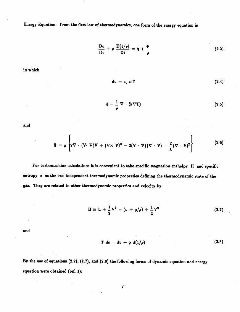
Energy Equation: From the first law of thermodynamics, one form of the energy equation is
Du + P D(1/p) _el+_ _Dt Dt p
(2.3)
in which
du = cv dT (2.4)
_1 = _1 V. (kVT) (2.5)P
and
t=#
l2
(v • v)2[v)v + (v× v)2 - 2(v. v)(v. v) - J
(2.e)
For turbomachine calculations it is convenient to take specific stagnation enthaipy H and specific
entropy s as the two independent thermodynamic properties defining the thermodynamic state of the
gas. They are related to other thermodynamic properties and velocity by
H = h + 1V 2 = (u + p/p) + 1V _2 2
(2.7)
sad
T ds = du + p d(1/p) (2.8)
By the use of equations (2.2), (2.7), and (2.8) the following forms of dynamic equation and energy
equation were obtained (ref. 1):

P+ _ v(v. v) +
3
(2.2a)
and
Dt p Ot p 3
(2.3a)
In the case of steady invicid flow, equation (2.2a) becomes
V x (V x V) =VH- TVs (2.2b)
which is the Coroco equation originally deduced for the investigation of flow with shock and vorticity.
The second law of thermodynamics states
TDs>_ 1Dt
(2.9)
Combining equation (2.8) with the first law of thermodynamics, equation (2.3), yields
T Ds =_i+ #Dt p
(2.1o)
which conforms with the second law of thermodynamics, equation (2.9).

From theprecedinggeneral,basicequationsthe followingcanbenoticed:
(1) In the stationaryframeof referencethe flowunsteadinessis representedby the partial derivative,
with respectto time, of densityin thecontinuity equation, of velocity in the dynamic equation, and of
pressure in the energy equation.
(2) Stagnation enthalpy is, in general, affected by the viscosity of the fluid through the last two
terms on the right elde of equation (2.3a). If the last term on the right side of equation (2.1a), the
viscous force per unit mass of fluid, is denoted by Ff, then the two viscous terms in equation (2.3a) are
O/p and V.Ff. Thusthe effect of viscosity on the stagnation enthalpy is not represented by V.Ff
alone.
2.2 Effect of Viscosity on Basic Equations
In order to more clearly see the effects of viscosity on the changes in stagnation enthalpy and
entropy, the dynamic equation (2.2a), the energy equation (2.3a), and the entropy equation (2.10) are
further examined using the stress tensor f (ref. 43).
Newton's Second Law of Motion
Let the resultant stress (force per unit area) acting on the surfaces of an infinitesimally small fluid
element be denoted by f (fig. 2.1) where r is related to the hydraulic pressure p, uniform in all
directions, and a viscous stress _r' by the following equation:
9

r!o x rxy rxs o_
_" ry x Gy ry s = ]Ty x
r,y o
(2.11)
or
1"ij = --p 6ij + r. _.IJ(2.12)
where
1, i=j
6_ : 0, i * j
The vector and tensor form of Newton's second law of motion are, respectively
DV 1,-, 1 ,=- -_vp -t- _V.r
Dt p p
(2.13a)
and
DV i aV i _V it
1 013 __ 1 arij (2.13b)
P_C i P O_Xj
where Einstein's summation convention is used.
• By using equations (2.1), (2.2), and (2.3), Newton's second law of motion can also be put into the
following form:
10
1 lJ_

8V _ V x (V x V) -VH + T x Vs + 1V.r, (2.14)
First Law of Thermodynamics
The first law of thermodynamics is, in general, expressed by
De_ = -, (2.15)Dt
The time rate of work done by the force acting on the fluid element surface, per unit mass of fluid,
as seen by a stationary observer is
p 8 Xi p _ Xi p 0 X i
or
, = _Iv.(f.V) = -_Iv.(pV) + _Iv • (_'.V)P P P
(2.16b)
where
• '-V = f._Vj (2.17)
The first term on the right side of equation (2.16b) can be written as
1 V.(pV)= 1 (V.Vp+pV.V) 1 {Dp _}P P P D-t
11

Substitutingthe continuityequation(2.1a)into theprecedingequation results in
n
p p (Dt p p Dt Dt p 8t
Substituting the preceding equation into equation (2.16b) results in
4" -- D(p/p) _ 10p + _1V- (¢'-V)Dt p _ p
(2.18)
To this observer the time rate of increase of internal energy is
De_Dt DtD {u+ _} (2.19)
Substituting equations (2.18) and (2.19) into equation (2.15) yields
DH _ lap +el + lV -(,'.V)Dt p & p
(2.20)
The energy equation (2.20) can be put into a slightly different form by expanding the last term on
the right side of the equation as follows:
, _, I,,p axi P [ _J ax i
l (2.21)
+ vj--_-T,I
12

But
aV__x'ij
axi
(2.22a)
and
1 a,-'_ = Ff (2.22b)
Therefore, the energy equation (2.20) can be written as
DH _ lop +_I+ _- +Ff. VDt p at p
(2.23)
which is the same as equation (2.39).
The energy equation (2.20) can also be transformed to the form of equation (2.3) as follows by
multiplying terms on the left side of equation (2.13b) by Vi:
D V 2 ap a_"i.i (2.24)___ : Vi -- - Vio_xi _)xjDt 2
Using equations (2.21), (2.22a), and the continuity equation (2. la), equation (2.14) is transformed into
the following equation:
__[pD(1/p)___]__ Dt'_DV_(2.25)
13

Substitutingequations(2.25)and(2.19)into the first law of thermodynamics,equation(2.14)resultsin
Du + P __D(1/P) = dl + #-Dr Dt p
which is identical to equation (2.3).
The physical meaning of this form of the energy equation can best be seen by deriving the equation from
the point of view of an observer moving with the fluid element. To this observer the time rate of the
increase of its internal energy is
De_ Du (2.26)Dt Dt
and the rate of doing work against the surroundings by unit mass of the fluid element per unit time is
lrijOV ! = 1( OVi _ i_i}
D(1/p) _
Dt p(2.27)
In equation (27) _r_ is the rate of work done by unit mass of fluid element as seen by an observer
moving with the fluid element and _i are the coordinates moving with the fluid element.
14

Substitutingequations(2.26)and (2.27) into equation (2.15) yields
Du[ (2.28)
Equation (2.28) is exactly the same as equation (2.21) which is obtained by modifying the energy
equation (2.26) obtained from the point of view of a stationary observer with the use of Newton's second
law of motion (eq.(2.13)).
It is important to notice the following:
(1) To a stationary observer, the rate of work done by unit mass of fluid against viscous forces and
the rate of increase of internal energy are, respectively,
-1V.(_'. V) and D(u q- V_/2) (2.29)p Dt
These two terms appear in the corresponding energy equation (2.20).
(2) To an observer moving with the fluid, the rate of work done by the unit mass of fluid against
viscous forces and the rate of increase of internal energy are, respectively,
Du_ and mp Dt
These two terms appear in the corresponding energy equation (2.28).
15

In the derivationof theenergyequationfrom the first law of thermodynamics,theexpressionfor
workdoneby the fluid elementagainstits surroundingsandthe increasein the internalenergyof the
fluid elementmust bewritten for the sameobserver,eitherstationaryor movingwith the fluid. If oneis
written for the stationaryobserverandthe otheris written for theobservermovingwith thefluid, the
resultingequationiserroneous.Unfortunatelythis kind of mixup hasappearedin somepublications.
Two-DimensionalLaminar BoundaryLayer Flow In order to clearly see the effects of fluid
viscosity and heat transfer on the energy equation and entropy equation, the following general analysis of
steady laminar boundary layer flow is made. The velocity and temperature distributions in the boundary
layer and an infinitesimally small element whose width and height are 5x and 5y are shown in
figure 2.2. The x and y coordinates are chosen, respectively, to lie along and perpendicular to the
tangent of the blade surface. The approximate relation commonly used to treat boundary layer problems
is employed in the analysis. Fluid pressure may have a gradient in the x direction.
(1) To a stationary observer, the time rate of work done by the fluid, per unit mass, is
@ -- _[m(p
JVxla _ a (_rV x Vy
_-P
(2.30)
and after employing the continuity equation
V4rD (p/p)
Dt(2.30a)
16
_:1I]

o
The time rate of heat transfer to the fluid element, per unit nmss, is
(2.sx)
Substituting equations (2.30a) and (2.31) into the first law of thermodynamics equation (2.15), the
following is obtained:
__._j - _I_ -+ =(2,s2)
Rearranging terms gives
DH N 1 k + +Dt p /)x
(2.33)
In equstion (2.33), .a'rV"(_ax
then becomes
is much snmJler than and can be neglected. Equation (2.33)
dH _ 1 B k B Vxat _ ÷(2.34)
17
If # = constant, Pr = 1, and the difference between V and V x is neglected, then equation (2.34)
becomes
H = constant everywhere in the boundary layer is a particularly useful solution to the above equation. In
this case, the wall temperature Tw equals the fluid stagnation temperature T o. When Cp of the gas is
a constant,
V 2T O = T + -- = constant (2.36)
2Cp
Differentiating equation (2.36) results in
_r = _ __v0v (2.37)i
_y Cp (_y
Itcan be seenfrom equations(2.37)and (2.31)that
(a)at the lower boundary of the boundary layer,V = 0 and aV/Sy > 0, therefore,r > 0 and
0T/ay = _ = o;
(b) at the upper boundary of the boundary layer, V = 71 and aV/Sy = 0, therefore, r = 0 and
_/_ =4=0;
(c)between thesetwo boundaries,aW/Sy > 0, r > 0,/Yr/Sy < 0, and therefore,heat transferisin
the y direction.
18

Since H = constant, equation (2.34) indicates that, under the present approximation, the amount of
heat transferred into (or out of) the fluid element is equal to thework done by the fluid element on the
surrounding (or by the external viscous shear stress on the fluid element), i.e.,
(2.38)
Of the two terms on the right side of equation (2.38) the first one is always negative and the second one
is always positive.
2. To an observer moving with the fluid the time rate of work done by the fluid element, per unit
mass, on its surrounding is
D(l/p) rlaW¢ + aW_ / = P D(1/p) _ r aVx (2.39)
where _ and _ are coordinates moving with the fluid, with the velocity W. Since
(2.40)
Substituting equations (2.39) and (2.32) into the first law of thermodynamics, the following is obtained:
19

Substituting equation (2.41) into the entropy equation (2.61) results in
T
The preceding two equations give, respectively, rate of increase of internal energy and entropy in the fluid
element due to the work done on the fluid element by viscous force acting on the fluid element.
In the particular solution above, substituting equation (2.38) into equations (2.41) and (2.42) results
in the following equations, respectively:
D(1/p)_ # 02 V2X
Vu _ _ lVx _ P 0Y2 2 _ pD(1/P) (2.43)D'-'t - p _" p " D-t
and
T Ds 1 Or_ # 02 v2__ = _ _ Vx__ x (2.44)
Dt p 0y p 0y2 2
The first term on the right side of these two equations is always positive because Or/0y is always
negative.
In this example it is quite clear that
2O
_Ett l

(a) the rate of work done by the viscous forces on the fluid element, per unit mass, seen by a
stationary observer at rest is 1/p _rVx)/ay = 1/p (r0Vx/ay + Vx_r/ay), where the first term is
always positive and the second term is always negative.
In the particular solution above, because the work done by the fluid element and heat transfer to the
fluid element just cancel each other, the stagnation enthalpy remains constant along the relative
streamline.
(b) The rate of work done on unit mass of fluid by the viscous force seen by an observer moving
wi_h the gas is r(l/p) 0Vx/ay , which is always greater than zero. . _
1 Vx _r p D(1/p) in which the first term isIn the particular solution above, (Cl - @) = - P _ - Dt '
always greater than zero, thereby causing Du/Dt and Ds/Dt always to be greater than zero.
It is quite obvious that the work done by the fluid element seen by a stationary observer and by an
observer moving with the fluid element are not the same. In writing out the energy equation, they should
be used with the increase in internal energy of the fluid element seen by the same observer.
r_ F_
2.3 Basic Aerothermodynamic Equations Governing the Three-Dimensional Flow of a
Viscous Fluid Through a Rotating Blade Row
?
General basic aerothermodynamic equations governing the fluid flow through a blade row rotating at
a constant angular velocity were formulated in reference 3 for a nonviscous fluid, in which the entropy s
and a new thermodynamic property I, first called "modified total enthalpy _ and later named "relative
stagnation rothalpy" (ref. 44), were taken as the two independent thermodynamic properties defining the
thermodynamic state of the gas. Later this formulation was extended to viscous gases in reference 43.
Continuity Equation: From the principle of conservation of matter, the equation of continuity is
21

or
+ v.(p w)= 0at
v. w + DlnP_0 (2.45a)Dt
Dynamic Equation: For a blade rotating at a constant angular velocity w about the z axis, Newton's
second law of motion is
DW 1 1 (2.46)= w_r -I- 2w x W=- _Vp + _V. _'Dt p p
=
Where T' is the viscous stress tensor acting on a fluid element.
The relative acceleration in equation (2.46) can be written as
DW aW
Dt ataW 1 (V × W)+(W.V) W=_+_VW 2-w xat 2
(2.47)
Rothalpy and relative stagnation rothalpy are defined, respectively, by (ref. 44)
(2.48)
22
I !11
w2 (,,,r)2 W2I-i+m=h- +m
2 2 2(2.49)
By using equations (2.4), (2.8), and (2.49) the following form of Newton's second law of motion is
obtained:
0W_w × (v ×V)=-VI÷TVs- lye' (2.50)8t p
Energy Equation: The energy equation for fluid flow passing through a rotating blade can be obtained
from the first law of thermodynamics in the same manner as in the case of fluid flow passing through a
stationary blade row. First, from a stationary observer's point of view, the rate of work done by the fluid
element, per unit mass, against its surrounding is
, = - I_r • v = - I_F • (W + U)
I= - _V • (¢.W) - ;EF÷_r
p (2.51)
= Iv-(pW) - 1 V. (¢'.W) - _ D(¥_')
p p Dt
where U is the blade speed wr.
energy per unit mass is
To the same otmerver the rate of increase of the fluid element's internal
De-D{ u _] V[ u WZ+2W__r÷_2r2]_-_ + =_ +(2.52)
23

Substitutingequations(2.51)and (2.52)into equation (2.15) yields
DI _- _.l__aP+ _1 + _Iv • (_'.W)Dt p Ot p
(2.53)
+
Just as in the case of fluid flow passing through a stationary blade row, the energy equation in the
form of the preceding equation can be transformed into the form similar to equation (2.28). For instance
the dot product of W and equation (2.46) is
D W 2 Op _ W /_'iiDt_ --w. (_,- _ ×w)=w_ _ (2.54)
The last term in the preceding equation can be written as
(2.55)
and the dissipation function for the fluid element moving with respect to the rotating blade is
(2.56)
24
+l II

By using equations (2.55), (2.56), and the continuity equation (2.45); equation (2.51) can be transformed
into the following equation:
Substituting equation (2.57) and (2.52) into equation (2.14) yields the following form of the energy
equation:
D.0{D I,+DtAgain the physical meaning of this form of energy equation can be seen more clearly by deriving the
equation from the point of view of an observer moving with the fluid element. To this observer the time
rate of the increase in the internal energy is given by equation (2.26) and the time rate of work done by
the fluid element against its surroundings is
1 awl D(1/p) _' (2.59)= - lrij__= p_ - __* p Cg_i Dt p
where _ is the coordinate moving with the fluid.
Substituting equations (2.59) and (2.26) into equation (2.14) yields equation (2.58).
25

EntropyEquation: From the second law of thermodynamics,
T __Ds__ _t (2.60)Dt
substituting (2.58) into the entropy equation (2.8) the following is obtained:
T __Ds= ¢1 + --#' (2.61)Dt p
Equations (2.53) and (2.61) are two important equations. They appear quite similar to equation
(2.20) and (2.10), respectively, but the total derivative with respect to time now means following motion
along the relative streamline, and the partial derivative with respect to time now refers to the derivative
at a coordinate point relative to the rotating blade.
2.4 Steady Fluid Flow Through a Stationary Blade Row and
Steady Relative Flow Through a Rotating Blade Row
Under steady operating conditions, fluid flow through a single stationary blade row is steady and the
unsteady terms in the governing equations can be neglected. Similarly under steady operating conditions
fluid flow through a single rotating blade row is steady and the unsteady terms in the governing
equations can be neglected. However, even in a single-stage turbomachine, there is always a stationary
blade row upstream (in the case of a turbine) or downstream (in the case of a compressor) of a rotating
blade row. Usually they are spaced not too far apart and the fluid flow relative to either blade row is
26
1 I I

unsteady. Because of the mathematical difficulty, in practically all of the design calculations and analysis
calculations, fluid flow relative to either the stator or rotor, is assumed to be steady.
Steady absolute flow in stationary blade rows means that the unsteady terms in governing equations
(2.1), (2.14), (2.20), and (2.28) at a fixed coordinate point, say (r,0,Z)o are equal to zero.
In the case of fluid flow through a rotating blade row, steady relative flow means that all of the
partial derivatives with respect to time in governing equations (2.45), (2.50), (2.53) and (2.61) at a fixed
coordinate point, say (r#,Z)o , with the origin of the coordinates fixed in the blade (i.e., _ = 0 -_t), are
equal to zero. Furthermore, since the absolute velocity V is related to the relative velocity W by
v = w + u (2.62)
or
V r = W r ]
V z = W z
V o = We + osr
(2.63)
When the relative velocity at a relative coordinate point (r#,z)is steady, the absolute velocity at a
relative point, Vr,4, z is also steady with respect to the rotating blade, so is V x V.
Because the absolute flow is calculated for the stationary blade row, whereas the relative flow is
calculated for the rotating blade row, there is an abrupt change in the tangential component of the fluid
velocity, and consequently, in the streamline when the fluid motion is referred to the different coordinate
27

system moving from one blade row to the next (fig. 2.3). However, the projection of the streamlines on
the meridional plane is continuous because the meridional components of the absolute and relative
velocities are continuous (fig. 2.4).
In the following presentation, as well as in computer codes, only the governing equations for steady
relative flow through the rotating blade row will be given. It is understood that when the blade row is
stationary, w = 0, _ --, 0, W _ V, I -, H, and t' --, i.
2.5 Viscous Terms in the Governing Equations
An analysis will now be made on the magnitude of the viscous terms in the governing equations.
Continuity Equation: For steady flow the continuity equation (2.45) becomes
v. (pw) = 0 (2.64)
Equation (2.64) does not contain a viscous term. The effect of viscosity on the fluid flow comes through
the entropy increase in the flow in the following equation of fluid density:
Pb (I-W2/2 -{- U2/2_ _-Z_-Ie
z: -w,/----,;(2.65)
The effect of entropy increase in density is quite large and consequently cannot be ignored.
Energy Equation: Of the two forms of energy equation (2.53) and (2.58), it is more convenient to use
(2.53). For steady flow it becomes
28
-71 r-

DI = _1 + 1 V (_'.W) (2.66)Dt p
In the core region the viscous stress and heat transfer are negligible. In the boundary layer region near
the blade surfaces and hub and casing walls, if the boundary layer is laminar, the Pr number of the fluid
is equal to unity, and the boundary walls are adiabatic walls, the viscous work term and heat transfer
term cancel each other. In actual turbomachines the boundary layer flow is turbulent and the Pr number
is different from 1, and the summation of these two terms will not be equal to zero, but the magnitude is
expected to be small. The following equation is usually considered to be a good approximation for the
entire flow region:
DI__ = 0 (2.67)Dt
Dynamic Equation: For steady flow equation (2.34) becomes
1W x (V x Y) =VI- TVs +- V._' (2.68)
P
When I is taken to be constant on all streamlines, the magnitude of VI depends on the magnitude
of VI at the inlet. Vs is quite small in the core region, but quite large near the solid wall. For
instance the radial entropy profile at the exit of a rotor blade row may look something like that shown in
figure 2.5. From the dynamic equation in the radial direction.
29

When the viscous stresses are neglected, equation (2.68) is simplified to
W × (V x V) = VI - TVs (2.69)
Equation (2.69) in the radial direction is
0W s W_ a(V#r ) OWr aI Os (2.70)W s "-- + W z- + -- -- T--
Or r Or 0z Or Or
The effect of radial entropy gradient on the radial variation of velocity is indicated in figure 2.5.
The inclusion of entropy gradient in the dynamic equations is necessary for a better prediction of velocity
variations near the solid wall.
Entropy Increase: Evaluation of entropic increase along the streamlines by equation (2.61) requires
a solution of the complete set of governing equations for viscous fluid. At the present time approximate
value of entropy increase along the streamlines may be estimated by an appropriate value of the
polytropic exponent of a polytropic process which represents the actual flow process (ref. 1). It may also
be estimated by the pressure recovery factor and the isentropic rotor efficiency obtained in experimental
investigation and tests (ref. 47). For the flow through a stator blade row the entropy increase across the
blade row is calculated from the recovery factor in stagnation pressure as follows:
sc _ Sb = R "/ ln_l (2.71)_-1 a
or
=i
3O

s c -- sb = R _ in Pb______ (2.71a)- 1 Pco
For the flow passing a rotor blade row, the increase of entropy across the blade row is calculated from the
isotropic rotor efficiency as follows:
Sb -- Sa = R _ In Tb°/Ta° (2.72)
7-1 1 + _(Tb°/Tao- 1)
where
= _/s for compressor rotor
:1/_[ s for turbine rotor
2.6 Some Remarks on the Energy Equation and the Entropy Equation
The First Law of Thermodynamics and the Second Law of Thermodynamics are two important
physical laws governing the flow of a compressible visCous fluid in a turbomachine. The following
remarks are made here regarding the energy equation and entropy equation derived from these two laws.
1. Energy equations in two different forms were described in Section 2.1 and 2.2 for flow through, a
stationary blade row and a rotating blade row respectively. In one form of the energy equation, equation
(2.28) or (2.58), the increase of internal energy of a fluid element along the streamline is given directly by
the heat transfer from the surroundings to the fluid element minus the work done by the fluid element
against its surroundings. The equation is the same as the one universally used in thermodynamic
31

calculations,exceptthat there is an additional work done term by the fluid element against the external
viscous force. In the other form of energy equation, equation (2.2) or (2.53), however, the increase of
stagnation enthalpy or stagnation rothalpy is given by three terms, namely, the heat transfer to the fluid
element, the work done by the fluid element against the viscous forces, and an insteady pressure term. It
shold be noted here that the work done by the fluid element against external pressure is included in the
first form of the energy equation, but not in the second form of the energy equation. (Equation (2.18)
will help to explain this difference.)
2. It should be emphasized that the heat transfer term (t refers to the heat transferred to the fluid
element from its surrounding fluid elements and that it is not equal to zero for the fluid element in the
viscous region, even when the flow of the fluid as a whole is adiabatic, i.e., there is no heat transfer
between the fluid and the bounding wall. For instance, in the preceding analysis of a two-dimensional
boundary layer flow, it is seen that (i) there is a positive heat transfer into the fluid element in the
boundary layer, and (ii) when the Prandtl number of the fluid is equal to one, this amount of heat
transfer into the fluid element is equal to just the work done by the fluid element against the viscous
forces acting on the fluid element, thereby keeping the stagnation enthalpy constant along the streamline.
This is a very useful result, which provides a sound basis in taking stagnation enthalpy or stagnation
rothalpy constant along the streamline in current engineering calculation for turbomachine flows.
Because of this canceling effect, it should be kept in mind that when the viscous effect on the stagnation
enthalpy is considered in the calculation, it is not correct to keep one viscous work term in equation
(2.20) or equation (2.53), or two viscous work terms in equation (2.23) and to neglect the heat transfer
term in these equations.
3. Entropy equation (2.10) or (2.61) clearly shows that the increase of entropy of the fluid element
along the streamline is made of two parts, namely the heat transfer to the fluid element (1 and the work
done by the fluid element against the external viscous forces as seen by an observer moving with the fluid
32

element,the dissipationfunction _ (see eq. (2.27)). Depending on the nature of problem, dl may be
positive or negative (usually positive), but 4_ is always positive.
4. The heat transfer term dl in the energy equation and entropy equation is heat transfer to the
fluid element from its surroundings due to temperature difference. The viscous term in the energy
equation and entropy equation is work done by the fluid element against the viscous force acting on the
fluid element. They are independently evaluated according to their own definition, which is set up to the
heat transfer term and work done term in the First Law of Thermodynamics (eq. (2.15)). In light of the
preceding argument, it is easy to see that the frequently-appearing saying awork done by the frictional
forces acting on the fluid element turns into frictional heat and is added to the fluid element,"
dH/dt = F[- V, T ds/dt --F?- V (for instance, eq. (3.19) on p. 51 of ref. 45 and equations in the
middle of p. 277 of ref. 46) are incorrect.
33

CHAPTER 3
GOVERNING EQUATIONS FOR FLUID FLOW ALONG RELATIVE STREAM FILAMENTS
3.1 Following Fluid Flow on Relative Stream Surfaces
In order to solve the steady three-dimensional irrotational or rotational flow in a relatively simple
manner, an approach was taken in reference 3 to obtain the three-dimensional solution by an appropriate
combination of mathematically two-dimensional flows on two different kinds of relative stream surfaces
(figs. 3.1 to 3.3). The first kind of relative stream surface is one whose intersection with a z-plane, either
upstream of the blade row or somewhere in the blade row, forms a circular arc (fig. 3.1). The _econd
kind of relative stream surface is one whose intersection with a z-plane, either upstream of the blade row
or somewhere inside the blade row, forms a radial line (fig. 3.2). These two kinds of relative stream
surfaces were designated as stream surface S1 and $2, respectively.
STREAM SURFACE OF THE FIRST KIND--S 1
Shown in figure 3.1 is a stream surface of the first kind formed by fluid particles lying on a circular
arc ab of radius oa upstream from the blade row. It is a generalization for three-dimensional flow
from the cylindrical surfaced usually considered in the two-dimensional design of turbomachines.
STREAM SURFACE OF THE SECOND KIND--S 2
A stream surface of the second kind is shown in figure 3.2. The important surface of this family is
the one that lies about midway between two adjacent blades, and divides the mass flow in the channel
formed by the two blades into approximately two equal parts. This surface is designated as the mean
34

streamsurfaceor mid-channelstreamsurface S2,m. For blades with all radial elements, such as the one
shown in figure 3.2, it is convenient to consider a mid-channel stream surface formed by fluid particles
originally lying on a radial line ab upstream from the blade row. Otherwise the radia! line is chosen
about midway in the passage with the fluid particles originally starting out from a curved line upstream
from the blade row as shown in figure 3.3.
In general, both of these two kinds of stream surfaces are employed in the solution of the three-
dimensional problem flow field in turbomachines. The correct solution of one surface requires some data
from the other, and consequently, successive solutions between the solution of one of these two surfaces
are involved. Yet, the solution of flow on each surface is manageable with the efficient technique for
mathematically two-dimensional problems.
Relations Among Relative Velocity of Fluid, Coordinates
of Stream Surface, and Normal to Stream Surface
In general, the coordinates of the relative stream surfaces, the components of the unit normal n
(figs. 3.1 and 3.2), and the velocity components are related by the following equations:
S(r, z) = 0 (3.1)
nrdr + ncd_ + nsdz = 0 (3.2)
nrW r + n¢W¢ + ns dz = 0 (3.3)
35
3.2 Equation Governing Fluid Flow Along S2
Stream Surface of S2 Stream Filament
Because S_ stream surface involved in the three-dimensional flow calculation is always a general
twisted surface, whereas the S 1 stream surface involved can be a surface of revolution, the S2 stream
surface will be considered first in the following treatment.
When the fluid motion on S2 stream surface is followed, equations (3.1) and (3.2) are used to
eliminate one of the three independent variables, the Io coordinate. That is, any quantity q on S2 is
now considered as
q -- f Jr, z, _o(r, z)] (3.3a)
The change in the quantity q along S2 due to a small change in r while z is held constant is (see
fig. 3.4)
(3.4)
Substituting a_o/0r from equation (3.2), for dz : 0, into the preceding equation gives
aq = &l _ nr 1 aq
ar & n@r_
in which the bold partial derivative sign is used to indicate this differentiation following the stream
8urfsce.
(3.4a)
36

Similarly,
Oq _ Oq nl 10q
Bz Oz n¢ r O_
(3.5)
Along streamline on S2
Dq = Wraq + W OqDt Or 0z
(3.6)
Continuity Equation
When the fluid motion is followed along the S2 stream surface and equation (3.4) and (3.5) are
used, the continuity equation for Steady relative motion becomes
_ + : p C(r, z)r Or az
(3.7)
where
OW rC(r, z) = -- 1 + nr + n_ntor 0_o
OW_° n OWI/+ (3.81
This continuity equation is put into the following form:
+ =0Or Oz
(3.9)
37

by using an integratingfactor B, which isrelatedto C by the followingequation:
Oln BDInB _ Wr 01nB + Wz _ = -C (3.10)Dt Or 0z
or
an_B=_;iodt=_f _cdxB i LiW
(3.11)
Equation (3.9)isthe necessaryand sufficientconditionthata stream function k_
relatedto velocitycomponents by
exists._ is
8_----rBpW s (3.12a)
Or
-: rBpW r (3.12b)8z
The differencein • at two points j and k on the S2 surfaceis
_k_ t j = J_j d_ = j_j rBp(Wsdr - Wrdz ) (3.13)
The preceding equation indicates that B is proportional to the angular thickness of a thin stream
filament whose mid-surface is the stream surface S2 considered herein and whose circumferential
thickness is equal to rB. Indeed, if the mass flow into and out of the element of such a stream sheet (cut
between two planes normal to the z-axis, and a distance dz apart (see fig. 3.5)) is equated to zero, and
the distances dr and dz approach zero as a limit, the following equation is obtained:
38

(rPWr)+ =0
ar _z
Comparing this equation with equation (3.9) and considering the mass flow relations show r to be
proportional to rB. This proportionality means that physically B is a quantity which is proportional
to the angular thickness of a stream filament whose mid-surface is the S 2 surface considered herein.
With this interpretation, B is immediately seen to be closely related to the angular distance between two
adjacent blades. In actual calculation, only the ratio rB to (rB)i or r to ri is important. In general
it is easier to obtain the variation in rB from the distance between adjacent streamlines obtained on S1
surface than to evaluate B/B i by equations (3.11) and (3.8) using data obtained on S1 surfaces.
It is seen from the preceding section that in following the fluid flow along a stream surface, a
consideration of conservation of matter automatically changes the fluid flow on the stream surface to the
fluid flow along the stream filament. In general three-dimensional flow, the thickness of the stream
filament changes with respect to the two coordinates r and z. In the case of S2 stream filament (see
fig. 3.6) it is easy to see that: (1) in the radial direction, r increases with the radius as the
circumferential distance between the adjacent blades increases in the radial direction and (2) in the flow
direction, due to the blade thickness, r decreases as the fluid enters the blade channel and then increases
as the fluid moves toward the trailing edge of the blade.
Dynamic Equation
For general rotational flow, the dynamic equation (2.69) in the three perpendicular directions are
(3.15a)
39

/ awWr/a(V°,)aWr W. =- ---- (3.15b)
(3.15c)
In following the motion on S_ equation (3.15) are reduced to the following forms by using equations
(3.3) to (3.6):
a(Var)[
W_ + Ws _aWr aWs / aI + TaS + Fr
--_-r) Or Or
(3.16a)
(3.16b)
/aWr awffi] w_o a(V.r) ai +T as +F a
-- Wr(--_ - -- --oar) -- -r _z -- - O-z oa-'_
(3.16c)
where F is a vector having the unit of force per unit mass of gas defined by
(3.17)
40
llV
3.3 Principal Equation for Fluid Flow Along S2 Stream Filament
By considering the fluid flow along an S2 stream filament and using the partial derivative of fluid
quantities as functions of two independent variables r and z, the principle of conservation of matter
leads to the continuity equation given by either equation (3.9) or (3.14), which are the necessary and
sufficient conditions for a stream function _ to exist. The relative velocity components Wr and Wz
are related to the partial derivatives of • by equation (3.12). When this relation is used, the dynamic
equation in the radial direction can be used to form a principal equation governing the fluid flow on S 2
stream filament. The solution of the fluid flow on S2 stream filament is concentrated on solving this
principal equation for the single dependent variable 9. It is much better than solving a number of
dependent variables from a set of partial differential equations. The form of the principal equation will
be given for the direct problem and the inverse problem in the next two sections.
Principal Equation for Direct Problem
In the direct problem the shape of the S 2 stream surface is given. In practice the shape is specified
by a number of coordinate points lying on the surface, The components of the unit normal are then
calculated by equation (3.2) as follows:
Along the intersection of the S2 surface and a constant-z plane
(3.1s)
and along the intersection of the S2 surface and a constant r-surface
41

n IIW_--ro(3.19)
Components nr, n7_, and n s are determined by the preceding two equations along with the following
equation:
2 + n 2 + n2 =1nr _o I
(3.20)
Let
/znr Fr
n,_ F_
(3.21a)
ns Fz
n_ F_
(3.21b)
From equation (3.3)
W_o-- -(pW r -_-pWl)(3.22)
Using equations (3.21a) and (3.21b) and other basic relations, the dynamic equation in the radial
direction can be transformed into the following form (ref. 48).
42

1 w-7]+,,,)_(,+,,,+,,,) _ __,,+(,+,,,+,,,)WrW,1_,ar 2 s 2 ]ar az
+ ' +"')- (' +"'+ "').<.1_._ _r _.
(3.23)
where
1
+ -- _ __1_1[aI_ TaS
" I ar "_, r_ - _ ,,,,,_t_r _r
{
r_ 1 as+ l[aIM
I " f_(.+,.)ol... ,o.+_,_[ _ R az llitaz
,i Wi[ a_]+ - v a_._ -_aI t Or _i
+ wir + WrW_° a/_ar+ W_°Wl araV]]
+ Wr + W_° Oil + Wi_W ' c31,11a-_ T, )]
43

It is seen from the coefficients of the second order partial derivatives that when W > a or < a,
equation (3.23) is ]_yperbolic or elliptic.
Procedure of Solution for Direct Problem
In the direct problem of fluid flow along the S2 stream filament the variation of filament thickness
r (or rB) relative to its inlet value and equation (3.21) are given. There are nine independent equations
governing the fluid flow, namely equations (3.12a), (3.12b), (3.22), (3.16b), (3.21a), (3.21b), (2.67),
(2.71), or (2.72). The nine independent variables to be determined are Wr, W_, Ws, Fr, F_, Fz, I, S,
and @. (It may be noted here that, when equation (2.67) instead of the complete viscous equation (2.66)
is used for the energy equation in the calculation, there are only three independent equations among the
dynamic equations in three directions and the energy equation, because the latter can be obtained from
the former and the normality conditions between F and W.) The procedure of calculation is as follows:
(I) Starting from an estimated • field at the beginning of calculation or from the • field
determined in the previous cycle, compute Wr and Wz from equations (3.12a) and (3.12b),
respectively.
(2) Compute W_ from equation (3.22).
(3) Compute V 0 -_ W_ -t- _r and then F_ from the dynamic equation in the circumferential
direction, equation (3.16h).
(4) Compute Fr and Fz from equations (3.21a) and (3.21b).
(5) When the approximate equation, equation (2.67) is used for the whole flow region, stagnation
rothalpy I is taken to be constant along all streamlines.
(6) For an invicid isentropic calculation, entropy s is taken to be constant over the whole region.
For an analysis and design calculation, which tries to approximate the real flow as closely as
possible, a certain empirical variation along the streamline with the difference between the exit
and inlet value given by equations (2.71) or (2.72) is considered. In transonic turbomachines the
abrupt entropy increase across the shock is also taken into consideration.
(7) Solve k_ from the principal equation (3.23).
44
1_|1 -

Repeat calculations I to 7 until the desired accuracy is reached.
Principal Equation for Inverse Problem
In the inverse or design problem of fluid flow along the mid-channel S2 filament the variation of the
filament thickness r (or rB) relative to its inlet value is empirically determined by the desirable blade
thickness distribution. (In three-dlmensional solution the S_ filament thickness is taken from the
solution of S 1 filaments obtained in a previous cycle.) Now there are only seven independent equations
governing the fluid flow, namely equations (3.12a) and (3.12b), (3.16a) to (3.16c), (c), (2.67), and (2.71)
or (2.72), two less than that in the direct problem. On the other hand, however, there are nine
independent variables to be determined.
The differential of the coordinates of the S_ stream surface are related to the F components by
Frdr + F_ordlo + Fsdz = 0 (3.24)
In order for this differential equation to lead to an integral surface of the form represented by
equation (3.1), F must satisfy the following condition of integrability:
F.V×F=O (3.25)
Writing equation (3.25) in scalar form and using the relations (3.12a) and (3.12b) gives
45

_r(3.26)
By integrating along a constant r-line equation (3.26) gives
Fr/F/o- OttO,r/ (3.27)
If Fr=O ats 0
rLF_r )
(3.28)
Thus, there is only one degree of freedom left to the designer. Of all of the appropriate ways of
utilizing this degree of freedom, the one found most useful is to prescribe an appropriate variation of V 0
or V0r on the S2, m surface, i.e., the following equation is prescribed:
V a = G(r, z) (3.29)
The principal equation formed by combining the continuity equation and the dynamic equation in
the radial direction is
46
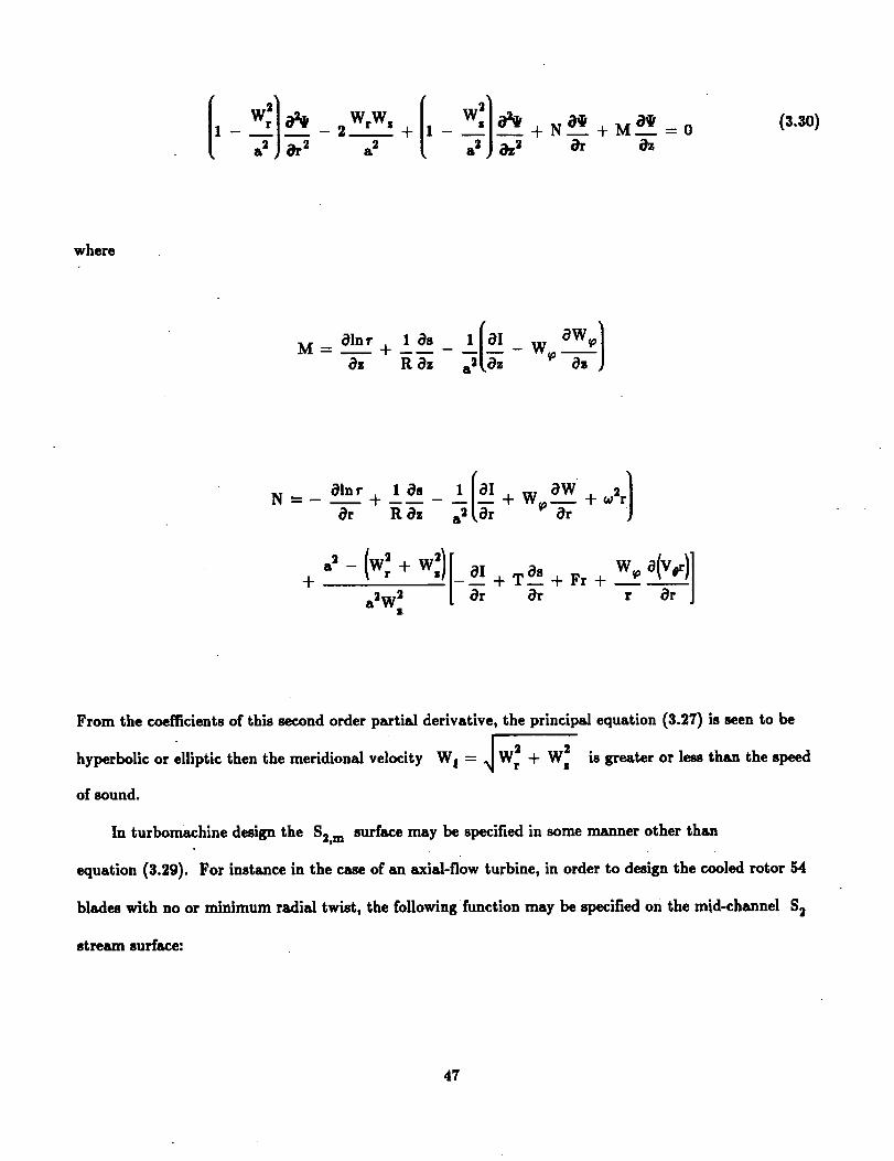
{1Wr/ WrW/- _,;_ - 2 _ + 1- a2;_2+N 8@_ +M a¢/ =o
Or 8z
(3._)
where
N _
+
81nr 18s 1(8I W 8W rl___/+ _ _ tg+ _,._g+_2
., (w:+w,)l- • 81 T 8s + Fr +
a2W 2 [- _ + Orr ")]--
From the coefficients of this second order partial derivative, the principal equation (3.27) is seen to be
hyperbolic or elliptic then the meridional velocity W! = J War + W2• is greater or less than the speed
1
of sound.
In turbomachine design the $2, m surface may be specified in some manner other than
equation (3.29). For instance in the case of an axial-flow turbine, in order to design the cooled rotor 54
blades with no or minimum radial twist, the following function may be specified on the mid-channel S2
stream surface:
47

w_ g_(') (3.31)Wl
In the case of a centrifugal compressor, in order to design the impeller blades with minimum deformation
and stress during operation, the mid-channel S2 stream surface may be specified to consist of all radial
elements, i.e.,
W_o
w---:- _g2(') (3.32)
In general then, the Sz stream surface n_y be specified by the following relation:
W_
W-":= g (r, z) (3.33)
By using equation (3.33) and other basic relations the dynamic equation in the radial direction can
be transformed into the following form (ref. 48):
w'_+ ' +N OlIl_+M _ -0
a2 J &_ Or &
(3.34)
where
48

N [1 a In B-(1 +.g21 +
+ a _ - W2 10I
a2W 2 ( &
/+ T_ +F r+2_oW_o |
Or ]
Procedure of Solution for Inverse Problem
The procedure of calculation of Sz, m stream filament is as follows:
(1) Starting from an estimated _ field at the beginning of calculation or from the • field
determined in the previous cycle, compute Wr and Ws from equations (3.12a) and (3.12b),
respectively.
(2) When (V#r)is prescribed, compute W lo from V 0. When (Wio/Ws) is prescribed, compute
Wto from equation (3.30) and Wz is computed from step 1.
(3) Compute Flo and Fs from, respectively, equations (3.16b) and (3.16c).
(4) When the approximate equation (2.67) is used for the whole flow region, the stagnation rothalpy
I is taken to be constant along all streamlines.
(5) For an invicid isentropic calculation, entropy s is taken to be constant over the whole region.
For an analysis and design calculation, which tries to approximate the real flow as closely as
possible, a certain empirical variation along the streamline with the difference between exit and
inlet value given by equation (2.71) or (2.77) is considered. In transonic turbomachines the
abrupt entropy increase across the shock is also taken into consideration.
49

(6) Solve @ from the principal equation (3.30) or (3.34).
Repeat steps 1 to 6 until the desired accuracy is reached.
3.4 Principal Equations for Fluid Flow Along S1 Stream Filament
The S 1 stream surfaces near the hub and casing walls are usually considered to be surfaces of
revolution. If the radius of the hub wall increases (or decreases) in the flow direction while the radius of
the casing wall decreases (or increases) in the flow direction, the S1 surface in the mid-span region may
be close to surface of revolution. Just like in the case of Sz flow, the continuity equation requires that
the mass of fluid flow in a thin stream filament be conserved. ' _.......................
The flow equations expressed by a set of orthogonal curvilinear coordinates (#, p) (fig. 3.6) are as
follows (refs. 2 and 4):
Continuity Equation:
at a_(3.35)
,. W relations
= - rpWto (3.36a)
50
':1-11/
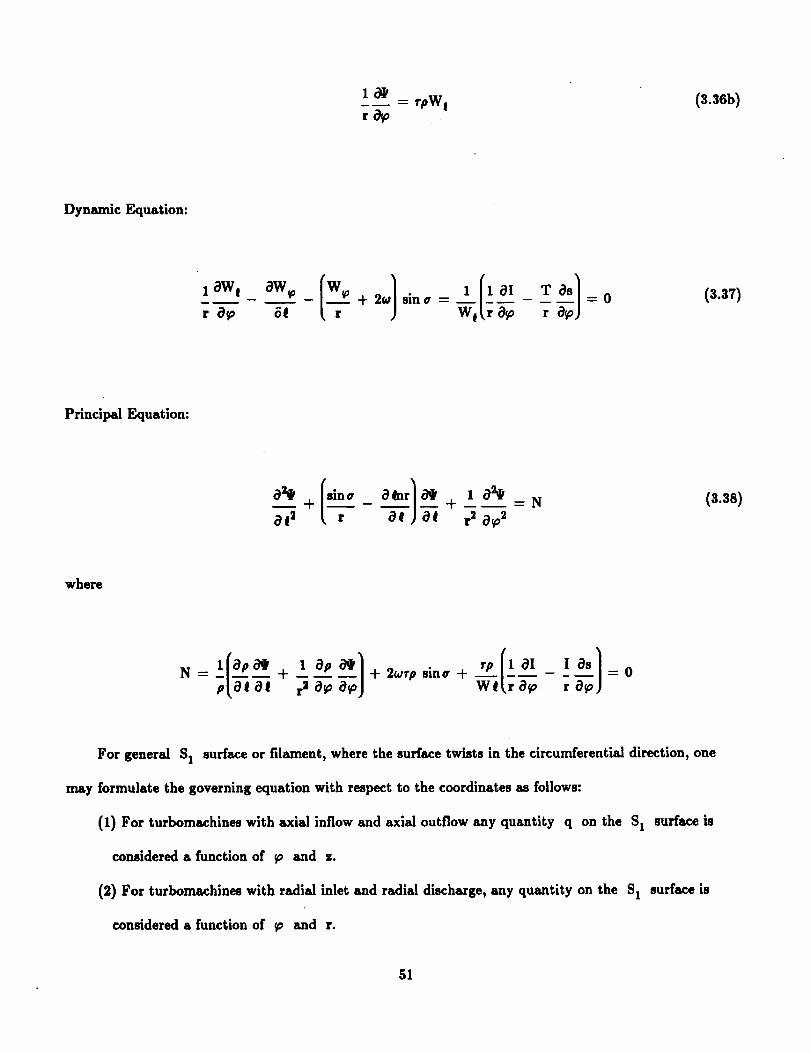
1 _ _ rpW! (s.sob)
Dynamic Equation:
1 8W!
r 8_sin o = -- =0
r
(3.a7)
Principal Equation:
o aCnrl_ 1 a21Ii+ _ ÷
012 r --_-) _-'_ r2 a_o2
-N (3.38)
where
For general S 1 surface or filament, where the surface twists in the circumferential direction, one
may formulate the governing equation with respect to the coordinates as follows:
(1) For turbomachines with axial inflow and axial outflow any quantity q on the S1 surface is
considered a function of to and z.
(2) For turbomachines with radial inlet and radial discharge, any quantity on the S1 surface is
considered a function of to and r.
51

(3) For turbomachineswith axial (or radial) inflow and radial (or axial) outflow, any quantity on
the S1 surface is considered a function of (Io, #).
(4) Same as that in case (3) but considered a function of noncurvilinear coordinates x 1 and x2.
52
!!! I I

CHAPTER 4
THREE-DIMENSIONAL FLOW EQUATIONS EXPRESSED IN TERMS OF
NONORTHOGONAL CURVILINEAR COORDINATES AND CORRESPONDING
NONORTHOGONAL VELOCITY COMPONENTS
Equations governing the fluid flow along S 1 and S 2 stream filaments were first derived in
references 2 to 4 employing orthogonal curvilinear coordinates (r, _, z) or (_,_, n). These equations have
been adopted in treatises on turbomachinery (for instance refs. 45 to 47), programmed into computer
cedes (for instance, refs. 8, 10 to 19, 22, and 23) and used in analysis and design of turbomachines (for
instance, refs. 21 to 26). During calculation of actual engineering problems it soon becomes evident that
in order to improve the relatively low accuracy of numerical differentiation (ref. 27) occurring at grid
points, unequally spaced near a curved boundary the coordinate line may coincide with the lea_iing and
trailing edges of the blade (see fig. 4.1) and a computer code may be used universally for turbomachines
of different geometry. Work to employ general nonorthogonal curvilinear coordinates for the calculation
of fluid flow along S1 and S_ stream filaments began in the sixties (refs. 28 and 29). Presented in the
following sections are some basic relations of general nonorthogonal curvilinear coordinates, equations
governing fluid flow along S1 and S2 stream filaments employing general nonorthogonal curvilinear
coordinates and the methods of solution.
4.1 General Curvilinear Coordinates in a Three-Dimensional Space
Let (yl, y2, y3) be the usual orthogonal Cartesian coordinates of point P and (x 1, x2, x3) be its
nonorthogonal curvUinear coordinates. In general the square of the element of arc ds is
53

where gij
ds2 = gijdxidxJ (i, j = 1, 2, 3)
is the covariant metric tensor of the three-dimensional space
(4.1)
gij-- ayk ayk ----el "ej = gjiax_ axj
(k = 1, 2, 3) (4.2)
gij = _ cos Oij (4.3)
where 0ij is the angle between the two basic vectors • l and el.
8A'e
The lengths of the elements of arc measured along the coordinates lines of our curvilinear systems,
ds(i} = g_ii dxi(4.4)
The element of volume dv is
dv = _g"gdxidx2dx 3 (4.5)
where g is the determinant Igijl. Let e! denote the reciprocal base vectors defined by
54
1 1_

(4.6)
The corresponding contravariant metric tensor of the three-dimensional space is
g_J_ G_j_ _. j = gJ_g
(4.7)
where Glj is the cofactor of the element gij in g.
For both systems it is convenient to use base vectors of unit length defined by
ui:ei+ g_'-_ (4.s)
ui ei --_ (4.9)
A vector B in the three-dimensional space is now either expressed in terms of the base vectors • l
and ui, or the reciprocal vectors e i and ul, as follows:
B = biei (4.10)
55

B = Bitti (4.11)
B = (4.12)
B = Biui (4.13)
where b i and B i are, respectively, the contravariant components and the physical components along • i
of the vector B; and b i and B i are, respectively, the covariant components and the physical
components along el of the vector B. The covariant component and its corresponding physical
component can be calculated from the contravariant component with the following formula:
bi --- B • ei = gijbJ (4.14)
Finally the differential operators in general curvilinear coordinates are as follows: the gradient of a
scaler I is given by
VI = e| __aI (4.15)Ox i
the divergence of vector W is
56
:l|!

° W (4.16)
and the contravariant components _i of vector E = V x V = _ie i are
_1 _ ! f av3 -- _V2 /
ax3j
1 av2_ _1]e= _-g axl _x 2
0
t:
(4.17)
4.2 General Curvilinear Coordinates on a Surface
In the investigation of fluid flow along an S l or S2 stream filament the governing equations are
written for the fluid flow on the mld-surface of the filament. Such a surface is a two-dlmensional
manifold embedded in a three-dimensional enveloping space and is usually described by coordinates ua
(a : 1, 2), called the curvilinear or Gaussian coordinates on the surface.
Under this notation the relevant equations corresponding to those in the preceding section are as
follows:
57

as2 = aa# dx a dx E (a, B = 1, 2) (4.18)
where aa# is the covariant metric tensor of the surface
aa_ = -- •a. ep----a_a (4.19)
aa#--_ cos #a_(4.20)
The lengths of elements of arc measured along the coordinate lines are
ds(a) -- a_aa dxa(4.21)
An element ofarea dA is
dA : _-adu ldu 2(4.22)
where a isthe determinant laa_l.
a = lao#l= a11a22sin2012 (4.23)
58

The contravariant metric tensor of the two-dimensional surface is
aO_ _- ea . e s -_ a_
all -- - a = la11sin20 2)-!
= all --,"--a =
(4.24)
= ---_ --a12 -- a _ --cos 012// a22 sin 2 012(4.25)
In the investigation of S 1 and S 2 flow employing nonorthogonal curvilinear coordinates the two
Gaussian coordinates, u I and u 2, on the surface, are selected to be the same as two of the three
curvilinear coordinates in the three-dimensional space. For instance, in the case of S 1 flow, x 1 and x 2
shown in figure 4.1 are two nonorthogonal curvilinear coordinates of the three general curvilinear
coordinates referring to the three-dimensional space and are the same as the two Gaussian coordinates
which refer to the two-dimensional surface. The third coordinate x 3, which refers to the three-
dimensional space, may be selected as normal to the x 1 - x 2 surface. In that case W 3 = w 3
W 3 _ w 3 -- 0.
In the following, distinctions between (u 1, u2) and (x t, x 2) will not be made, but ea, aa/_, a... (a,
= 1, 2) will be used for the S 1 surface, whereas el, gij, g • • • (i, j = 1, 2, 3) will be used for the three-
dimensional space in which the surface is embedded. For a given problem, aa/_ are computed from
equation (4.19) through numerical differentiation.
59
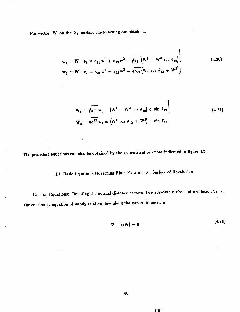
For vector W on the S1 surfacethe followingareobtained:
W1 = W. e I = aU wl -[- a12w2 = a_ll(Wl -}- W2 cos 012)
w2-- W- e2 = a21 wl -f-a_2w2--_--a_22(Wl co8 012 _ W 2)
(4.26)
(4.27)
The preceding equations can also be obtained by the geometrical relations indicated in figure 4.2.
4.3 Basic Equations Governing Fluid Flow on S 1 Surface of Revolution
General Equations: Denoting the normal distance between two adjacent surfacc_ of revolution by r,
the continuity equation of steady relative flow along the stream filament is
v • o (4.2s)
6O

Substituting equation (4.16) into (4.28) results in
_(_W'_H_,,)+0(,,W'_H_')=0Ox1 Ox2
(4.29)
This equation can also be obtained by considering the mass flow into and out of the elementary volume
(dSl, ds2, r) (see fig. 4.3).
When expressions (4.10), (4.15), and (4.17) are used, the dynamic equation (2.53) in the es
direction is
(4.30)
When equation (4.10) and the following relation between the absolute and relative vorticities are used:
V x V=V x W+2_ (4.31)
the dynamic equation in the e2 direction for steady relative flow is (fig. 4.4).
61

t ax'a 2J ax2
(4.32)
By using equation (4.26) the preceding equation becomes
ax"
= - 2 alt_-_22 e sino sin012 + Wt
(4.33)
This equation can alsobe obtainedby applying Stokestheorem to the surfaceelement offigure4.3,
Using relations(4.10)and (4.15)the energyequation (2.51)forsteadyrelativeflowbecomes
• aI el=w i al :oDI =W. VI =w%l" --:.D--t ax_ ax_
(4.34)
or
W 2 alDI W t al + ___--_ --0
(4.35)
SpecialForms of Flow Equations on St:
62

A number of useful special forms of equations presented in the preceding section can be obtained by
selecting a number of different x 1 - and x2-coordinate lines, as follows:
(a) xl-lines coincident with streamlines. In this case W 2 -- w 2 -- 0, W 1 -- W, equations (4.29),
(4.33), and (4.35) simplify to, respectively,
---a(rpW__V/_-22sin 0,2)=0ax 1
(4.29a)
_-_o )__X 1
(4.33a)
0I= 0 (4.35a)
ax I
If at the same time x 2 is taken to be normal to X1, the preceding equations are further simplified with
cos 012 = 0 and sin 012 = 1.
(b) xl-line coincident with the meridional coordinate line ! and x 2 - _o. In this case, 012 = 270 °,
W 1 --- Wi, W 2 = - Wto , _ -- 1, a_22= r, equations (4.29), (4.33), and (4.35) become those used in
references 4 to 9.
(c) S 1 surface is a cylindrical surface of radius r. If y = x 2 = r_o and x I - z, equations (4.29),
(4.33), and (4.35) become those of plane flow as used in reference 54. If, however, xl-line is taken to be
coincident with the streamline W l -- W, W 2 -- 0 and the equations are further simplified to
63

--_a(rpWa_2_sin _12)--0ax 1
(4.29c)
(4.33C)
aI= 0 (4.35c)
ax 1
Furthermore, if x2-line is taken to be normal to x 1 -line, an interesting result is obtained--the quantity
W _ is an invariant along an x 2 - line in the case where the variations of I and s along the x2-
line are equal to zero.
As seen in the preceding equations, dynamic equations (4.33) and (4.33a) contain the variations of I
and s of the fluid in the es direction. When they are uniform at the blade inlet and no change occurs
along the streamline, they are uniform everywhere--this is usually assumed on S1 flow calculation and
will also be assumed in the following discussion of methods of solution. In cases where their derivatives
are not' very small, they should, of course, be properly considered.
4.4 Methods of Solution for S1
When the xl-lines are corrected during calculation to coincide with the streamlines, equation (4.29),
along the xl-line, gives
64

a_22sin 012
/.-=-in which _/a22 and 012 are computed after each correction of the streamline coordinates. For
nonisentroplc flow of a perfect gas
i I 11i= _ e --_-= 1 - _ - 1 (pW)2 _-_ e---_-
_,., -T(_ i _ J(4.37)
The values of p and W can be determined from their product by rewriting equation (4.37) as (ref. 3)
2
(4.38)
where
S--8 i
R_= P e__
Pi
(4.39)
65

Thetablein reference3 canthen be used find _ (i.e., p) from the known value of _ (i.e., pW). W
then computed from pW after p obtained.
When the derivatives of I and s are neglected, equation (4.33a) yields
is
(4.41)
This equation is used to obtain a new set of values of W at the grid points by integrating along the
x2-1ines with the right side of the equation computed from known values of the preceding cycle. The
integration may be started from the mid-channel streamline as in references 4 to 6 or from the stagnation
streamline. The mass flow along the x2-line is then computed by
x2 012 a_-22 dx 2 {4.42)rh -- f(x2)0 rpW sin
A comparison between the computed mass flow and the correct mass flow leads to new values of
streamline positions. This process of correction should be applied at each station along the streamlines,
quite similar to the method employed in references 4 and 6. It may be noticed, however, that with the
use of the present nonorthogonal curvilinear coordinates the tangency of the relative fluid velocity at the
66

bladesurfacesis automaticallysatisfied.This method,of course,canalsobeemployedto modify existing
bladingor to designnewbladingas in references 4 and 35.
If it is desirable to keep the xl-line fixed during calculation, then
(1) pW 1 along the xl-line is corrected by the complete continuity equatiot_ (4.29).
(2) compute pW by
_w_E_w_)_+_w_)2 _w_)_w_)co__]'_ (4.43)
(3) integrate (W 2 a_11) along x I -line by
o(w_C) __ax2
_¢sin o sin 012 -f _xlC cos 012 -_ W 2)
ax2
(4.44)
(4) compute mass flow along x2-1ine by
rh -- j_('x2)0rpW 1 sin 012 x 2(4.45)
(5) correct the W 1 values at the grid points in the same manner as in the previous case.
67

Themethod described above is quite similar to that used in references 4, 6, and 54 except that the
solution of the latter is extended in the circumferential direction from the mean streamline by using a
Taylor series consisting of three terms. Whereas, the solution of the former is extended circumferentially
to successive streamlines by a Taylor series of only two terms.
In general the continuity equation and the dynamic equation are to be solved simultaneously through
the use of the stream function _. Equation (4.29) is necessary and sufficient condition that a function
exists with
= _rpW2 /all sinr--- 0120x 1
o_ = rpW 1 _f_sin 012ax 2
(4.46)
Substituting equations (4.46) into (4.33), the following principal equation governing the fluid flow along
the S 1 filament of revolution expressed in terms of nonorthogonal curvilinear coordinates x I - and x 2 is
obtained.
1 _II COS 012 _ 1 _ J o_ K _II-2 + + + -- M (4.47)
where
68

(¢ ) COS 012 0ln *" 1 _12aln _II/%2 I" sln _12 _{_ q_
I ' ) cos 012alnr 1 a$12K -- - 81n Ca22/a11 _"sin 012 + +
_22 _X 2 a_11 _X 1 sin _12 a_11 _X 1
M.._
+ - 2_arp sin a sin 2 012
Equation (4.47) may be considered as a generalization of the principal equation (3.38) in which the
orthogonal curvUinear coordinates (_, to) are used. When x I and x 2 become ! and to, respectively,
equation (4.47) reduces to equation (3.38).
When the _-derivatives are evaluated with suitable numerical differentiation formulas, including
those at the unequally spaced grid points (ref. 27) the resulting set of a large number of algebraic
equations involving the unknown k_'s at the grid points may be solved either by the direct matrix
method (refs. 3, 4, 8, 10 to 12, and 27) or by the relaxation method (refs. 3, 4, 10, 11, and 27). The
boundary conditions of the periodic variation of flow and the flow angles at the inlet and outlet stations
are to be satisfied in the same manner as described in references 4 and 8. Inasmuch as fixed (x 1, x 2)
coordinates are generally used in solving the principal equation (4.47), J and K are then a function of a
69

fixedgeometryand have to be computed only once. The exclusion of derivatives
right side of equation (4.47) is helpful in the convergence of the solution.
W I and W 2 on the
4.5 Equations Governing Fluid Flow on a General S2 Surface
Vorticity Equation and Dynamic Equation: In general, the problem of fluid flow along S2 stream
filament is treated in the same manner as described for S 1 stream filament in the preceding sections.
But there is an important difference in the S2 surface inverse problem in that the shape of the S2
surface is known only after the solution is obtained. Because of this and also for the elimination of the
angular derivatives in the governing equations, the independent variables, i.e., the nonorthogona|
curvilinear coordinates x 1 and x 2 are selected to lie on the meridional plane (see fig. 4.5) while
following the fluid motion on the S2 surface in exactly the same manner as was done in references 3, 10,
and 11 in which orthogonal coordinates z and r on the merldional plane were used. The third
coordinate x 3 for three-dimensional flow is chosen to be the angular coordinate _, which is the same as
that used in the cylindrical coordinate system previously employed in references 3, 10, and 11.
Corresponding to this choice of x3, g_33 = r, g = r2a, g_= r-1, W 3=W_,w 3=W_-r,V 3--
V0, v3=V 0-r,W 3=W_,w 3=W_r,V3--V0 and v 3=V0r.
It was found in references 2 and 3 that it is more convenient to use the absolute vorticity than to use
the relative vorticity in treating the relative flow on S2 surface. Under the present nonorthogonal
curvilinear coordinate system, the three contravariant components of V × V (eq. (4.17)) becomes
7O

r ax_ _J
,,__:r_-a[ a_ 8x !
,,_ _,_,w,_w,]r _ ax' ax2j
(4.48)
By using these expressions, the three nonorthogonal dynamic equations in the e l directions are
ax2j --T-[_ _x_ J ax' ax--E(4.49a)
- °Wl/:_- T 8.___s
ax2j ax2 ax2(4.49b)
J _/_'22[ ax2 a--__J= _ - T_-._
(4.49c)
71

Alternatively theseequationsmay also be obtained by using the following expressions of the rectangular
components of W and V × V in the e l, e2, and e8 directions (see fig. 4.2).
W c = W Isin #12,Wd = W2 sin Or2, We = We (4.50)
c ) , I ow,1
_,=,--(_,)8,°,,, r_t_ - _ J
__=r,_ = _si" e,,[a,,' a,,'J
(4.51)
We notice that the form of equations (4.49) and (4.51) are quite similar to equations (19) and (75),
respectively, of reference 3 employing orthogonal curvilinear coordinates (z, r, Io), but that the w's are
now more complicated covariant components of the relative velocity W.
With different choices of x I - and x 2 -coordinate lines suitable for different problems, the general
form of equations (4.49) reduces correspondingly to a number of special forms. For instance, if it is
selected that
(1) xl-line is coincident with the projection of the streamline on the meridional plane, then
#1 = ¢, W2= 0, Wl= W_; and w 1 = a_llWl, w 2 = W: a_22cos 012, and equation (4.49)
becomes
72 ¸

o(w, ax 2
_ aI
ax 2
(4.52)
_',_HL _ - __ :_-T
(2) x1-line is coincident with the projection of the streamline on the meridional plane and xS-line to
be radial line normal to the z-axis, then 01 = o, 02 = O, 01z = 90 ° - o,
a = _cos o, w 2 = W! a_22 sin o, equation (4.51) becomes
73

_1 .__
3 ---
r _1_1a_2 cos ff
r _c(_ q
1 lo(w, si ,)(_r
(4.53)
and (4.49b) becomes
_r
= __0I_ T __0s (4.54)Or Or
and (4.49a) and (4.49c) remain unchanged. Equation (4.54) may be used to evaluate the change of W t
along the r-coordinate lines for axial-flow machines.
Under this coordinate system, the correct expressions of V x V in the r, _ and z directions in
terms of the rectangular components W_ and W_ or V 0 are
74

= _.lsin a + _2_r
o[ 1 a(V0r) 1 a(V0r)_ 1 aW,
_ : _3 = tan ¢ OW__ __W!- 1 OW!
O, rm cos o a_22 Or
r [a_22 Or 0_o
(4.55)
(c) x 2 -line is normal to
equation (4.51) reduces to
xI -line and01 =$2*O, then Wl = wl a_ll, W2_- W2 a_2z, a: _
r _L ax2
OxI ]
_x I
(4.56)
and (4.49) reduces to
75

v 22Laxl ax2 TL _ ax'= aI _ T _s
ax I ax 1
r _L oxI a_ J ax_ ax_(4.57)
acp
_ aI _ T as
a_ a_
If 0x2 = 9o° and 01 = 02 = 0, then _ = avf_-22= 1, equations (4.55) and (4.56) reduce to,
respectively, (19) and (95) of reference 3 in which the orthogonai cylindrical coordinates r, _, z are used.
(d) x2-1ine is normal to x 1 - line and xl-line is coincident with the projection of streamline on the
meridlonalplane, then 01-02--a,W 2=0,W 1= Wpw 1- W! a_11, w 2=0, _a = _11a22 and
equation (4.48) simplifies to
76
I|!

_2
,r a_lla22 ax 2
r a_ _
r a_1ia22 ax 2
(4.58)
and correspondingly
=1_ 1 O(Vor)
r _ Ox _
I
-=3 _ w
1 a(w, ax 2
(4.59)
It is interesting to notice that in the present coordinate system the components of the absolute vorticity
-=t and =3 contain only one term each, and that for flow, in which the absolute vorticity remains zero,
both Vor and W1 $/al1r--
to the angular coordinate
coordinate ! as the fluid moves through the blade passage.
simplify to
remain constant along the x 2 - line, while W l _ must vary with respect
_o according to the variation of Vgr with respect to the meridional
In this coordinate system, equations (4.49)
77

= real_ T m@s
0t a_
(4.60a)
r ax 2 .a_'.. 8x 2 8x 2 ax 2¥-1L
(4._b)
[= al _ T as
a_ a_
(4.60c)
4.6 Governing Equations for S2 with Independent Variable _o Eliminated
The unitvectornormal to the S2 surfaceisexpressedas
n = ni el = Ni ui (4.61)
the orthogonalrelationisexpressedby
niel • dxiel = nldX1 + n2dx2 + n_odlo--N 1 N 2
dx 1 + _ dx 2 + N_ordp =0 (4.62)
78

The derivative of fluid quantity on S2 stream surface with respect to x 1 or x 2 with the other kept
constant is
a a a ax 3 a a a__ a nl a a NI a=__ + --__ + __-___--__-
ax 1 ax 1 ax 3 ax 1 _x 1 a_ ax 1 ax 1 n_ a_ ax I N_r a_ a_
(4.63a)
8 a a ax 3 a a a_ a n2 a a N2 a- + =_ + _ =_ - _ =.__ _
8x 2 8x 2 ax 3 ax 2 8x 2 a_ ax 2 ax 2 n_ a_ ax 2 N_r a_ a_
(4.63b)
When equations (4.63) are used the continuity equation for steady relative flow becomes
ax--_ _-_(4.64)
where r is the circumferential distance between two adjacent S2 surfaces and the dynamic equations
become
1_tax_-_ + , _,-a_ _(4.65a)
79

T _as -f2ax 2
(4.65b)
w2 a(vf)D(Vs.r)_ W 1 8(V#') + --f_ = F_r
Dt a_ll ax 1 a_2_ c3x2
(4.65c)
Alternatively, these equations can be obtained by projecting the three components of equation (96) of
reference 2 in e1, • 2, • 3 directions. F in these equations is the same F of reference 2, fi being its
covariant components
F= n-,; n= - . = =N_r p a_
(4.66)
From equations (4.26),
_w 2!
ax I
I/='='-] Bco.,,,+ +w,co.,12) (4.67)
8O
:! !1:

Substituting equation (4.67) into equation (4.65) gives
_-:_2/_x-I_ _
+ -r 8x I
_sOI + T _ = -fl
Ox 1 8x 1
(4.68a)
+w2cos012) [(wl
w a,v.r,.IT.w'L- ; _ +_ Ox-_
(4.68b)
D(v°r)wl _,(vor)w_a(Vor)-- + = f_o = F_or
Dt a_11 ax I a_'-22 OX 2
(4.68c)
Equation (4.68b) is the most important equation for S2 flow just as equation (4.33) for S 1 surface
flow.
Corresponding to the different choice of the x 1- and x2-coordinates, equations (4.64) and (4.68)
reduce to the following special equations:
(1) xl-line coincides with the projection of the streamline on the meridional plane.
W 2 - 0 and equations (4.64) and (4.68) simplify to, respectively
81

a (,pwl _sin Ol,)= o(4.69)
and
W_ a(V#r) 01 + T 0s fx
r B! _C a_
(4.70a)
(4.70b)
D(V#r) = W! a(Vsr)
D't 1f-_" B-t =f÷=F_#r
(4.70c)
Equations (4.69) and (4.70b) of S2 surface are quite similar to equations (4.29a) and (4.33a),
respectively, of S 1 surface.
(2) xl-line coincides with the projection of the streamline on the meridional plane and x2-1ine is in
the radial direction normal to the z-axis. Equations (4.69), (4.70a), and (4.70c) remain
unchanged, but (4.70b) becomes
82
OR_,_ PAQE _SOf POOR OUALrnf
! 1!-

ar 8C W! [ r &
iOI as+ __ - T -- - fr|
ar Or J(4.71)
(3) xl-line coincides with the projection of the streamline on the meridional plane and x2-1ine is
normal to xl-line. Equations (4.64), (4.70a) and (4.70c) remain unchanged, but (4.64) simplifies
to
a(W!_ _ _[_ W_o a(Ver )ax 2 W! r ax 2
1
+ _OI _ T __0s _ f2[ax 2 ax 2 ]
(4.72)
It is noticed that equation (4.70b) contains an f2 term which is, in general, not equal to zero inside the
blade passage.
By the use of equations (4.63), the energy equation (4.35) becomes
DI W 1 OI W 2 OI-- + ----0 (4.73)
Dt a_-H/_x' a_22 Ox 2
For the special case where xl-line is coincident with the projection of the streamline on the meridional
plane it simplfies to
aI-- =0
ax I(4.74)
83

4.7 Methods of Solution For S2 Flow
Since the equations governing the flow along S_ stream filament are quite similar to those along S1
stream filament (the main difference being the difference in the partial derivatives involved), the methods
of solution are also quite similar. In the first group of methods of solution, W 1 or • is integrated along
successive x2-coordinate lines, whereas in the second group of methods of solution _-values at all grid
points on the mld-S 2 surface are solved at the same time.
In the first group, if the xl-lines are corrected during calculation to coincide with the projection of
the streamlines on the meridional plane, the continuity equation (4.64) gives
pw,-- (pwJ (r _ sin #12)i (4.75)
r a_22sin 012
S 2 filament flow is calculated by considering the effect of entropy increase in the density equation
/'" !/'1 V --_-Zi-1.-si
S= p -2 e"--R--
Pi
_b = 7 - 1 pW! Hi _---'i e R
(4.7e)
The values of p and W
of equation (4.38) with
can be determined from their product by rewriting equation (4.75) in the form
84

a(Wl a_ll) 2 [ W_oaiV0r) OI as ](4.77)
The tableinreference3 Can be used to find E (orp) from the known value of 4_(or pW#). W_ isthen
computed from pW_ after p isobtained.
The rightsideof equation (4.70b)ismore complicatedthan equation (4.41)of S1 flow, In the
inverseor designproblem, the variationof V0r isspecifiedby the designer,whereas in the director
analysisproblem itisobtainablefrom the given shape of the S2 surface(seenext sectionforfurther
discussion).The variationof I isobtained from itsinletvalue and equation (4.73).The variationof s
isestimatedfrom itsinletvalue and the empiricalequation. W t_ isthen integratedalong the x2-
linesfrom a streamlinealong the innerboundary or in the middle ofthe flowregionin the same manner
as that in the S1 surfaceflowcalculation.In the casewhere the x2-1ineischosen normal to the xl-line
itisconvenientto rewriteequation (4.72)as
rh-- K_f(x:2)h rpW! sin 012 a_"2_ dx 2(4.78)
and integrate (W! a_11) 2 along the x2-1ines. After variation of W_ along x 2 is obtained, the mass
flow along x _ is computed.
with
I_ c -2rr - Nt (4.79)
85

where _ is a correction factor as indicated by figure 19 of reference 7. If the range of integration
includes the wall boundary-layer regions, m calculated should be slightly greater than the actual mass
flow because the calculated velocity in the wall boundary-layer region is greater than the actual value (see
fig. 2.5). In the design problem we may either specify the mean streamline and obtain the coordinates of
the inner and outer boundaries from given mass flow, or specify one boundary and obtain the other
boundary. In the analysis problem, the mass flow calculation is used to correct the values of W# and p
on the streamlines (see ref. 6).
If it is preferred to use fixed xl-lines, then the variation of pW 1 along the x 2 -lines should be
corrected according to continuity equation (4.64). Compute pW by
I
(4.80)
integrate W 1 a1_1 along x2-1ine by
cos °121
(4.81)
compute mass flow along x2-line by
86

(4.82)
and correct W 1 values at the fixed grid points in the same manner as in the previous case.
Analogous to the Sl-surface problem, the continuity equation and dynamic equation may be solved
simultaneously through the use of stream function. From equation (4.64) a stream function can be
defined with
rpW 2f----
= _ _all sin 012i)x I
_II = rpW1 a_"22 sin 012
ax 2
(4.83)
Substituting equation (4.83) into the dynamic equation (4.65b) gives the following principal equation for
flow along S2 stream filament.
1 a:_ cos 012 _ 1 _ J _ K M-2 + + +
all a(xl) 2 _ axl _X 2 a22 _(x2) 2 _ _xl _ _x2
-- M (4.84)
where
87

J .._
Z _
) cos 012 aln r 1 a012aln _/all/a22 r sln 012 + +
_t_ t _ ax2 sinO_2_22 ax2
-- ) cos o12 aln r 1 aol2aln _]a_2/all r sin 012 + +
_-22ax2 _ axI sln012_-_ ax'
f. 1 alnp _ cos 01z aln Pl 1
°,1 ox2j llox1
+ 1 0 In p _ co_ 0_2o in p 1 _ + pC
ax 2 at/'_z_ ax2 J a_22 ax2
Equation (4.84)may be consideredas a generalizationof the principalequation (107a)ofreference3
where orthogonalcurvilinearcoordinates r,_, z are used. When xI and x2 become z and r,
respectively,equation (4.85)reducesto equation (107a)of reference3.
When the g-derivativesare evaluatedby suitablenumericaldifferentiationformulas ofequal or
unequal spacing(ref.27),the resultingsetof a largenumber ofalgebraicequationscontainingthe
unknown g-values at the gridpointsare obtained. Also the dynamic equation may be writtenas
ft ' WdL : f f (V× W)t o _(1a22 sin Ol2dxtdx2
1
_ O__I+ T O__s_ q[
Ox_ ax 2 ]dxldx 2
(4.s5)
and integration along 1, 2, ...,8, 1 around the grid point E results in an algebraic equation containing
the g-values at the grid points A,B,...,I, (fig. 4.7). The resulting set of algebraic equations containing
88
1 !1

unknown _-values at the grid points in the order of several hundred for one stream filament, can be
solved by either the direct matrix method or relaxation method as employed in references 3 to 8, 11
and 12.
4.8 Computation of F Term in Inverse Problem
It is pointed out in Chapter 3 that in the inverse or design problem the following condition of
integrability should be used in the solution in the fluid flow along the S2 stream filament.
F.v × F--0 (4.86)
When general curvilinear coordinates are employed, substituting equations (4.12), (4.17) and (4.63) into
equation (4.86) gives
(4.87)
Then
_-- __ dx 1+ X)o ax 2
(4.88)
or
89

a_F_0r io
(4.89)
The procedure of calculating f2 is similar to fr of references 2, 12 and 16. Compute fl from
equation (4.68a), f_ from (4.68c), the derivative of fl/f_ with respect to x 2, then integrate f2 along
x 1 from (X{)o, where f2 is known. It is convenient to choose (xl)o at a station where Fr is equal to
zero because F 2 can then be computed from F I.
4.9 Computation of Components of Normal and W_ In Direct Problem
In the direct or analysis problem, the known S2 surface offers two relations between the n- or F-
components. Since n is normal to W,
n • W = nl wl + n2w 2 + n_w_ --N 1 W 1 N 2 W2
+ + N_W_ - 0 (4.90)
or
NIW 1 sin 012 + N2W 2 sin 01_ + N_W_ = 0 (4.91)
then
9O
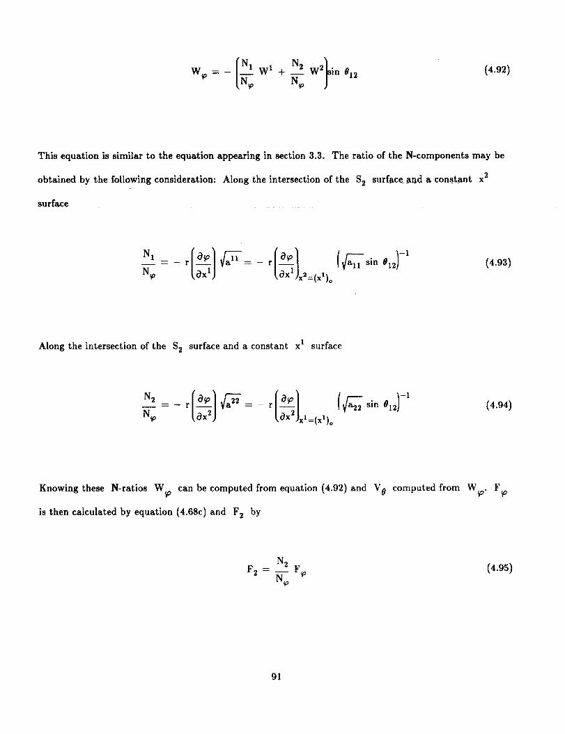
wlN2w2 i. (4.92)
This equation is similar to the equation appearing in section 3.3. The ratio of the N-components may be
obtained by the following consideration: Along the intersection of the S2 surface and a constant x 2
surface
(4.93)
Along the intersection of the S2 surface and a constant x 1 surface
N--_ r _x z (OX2)xl=(Xl)o
Knowing these N-ratios Wto can be computed from equation (4.92) and V 0
is then calculated by equation (4.68c) and F z by
computed from Wto. Fta
N 2
F z = _ F_N_
(4.95)
91

CHAPTER5
TWO- AND THREE-DIMENSIONAL SUBSONIC FLOW IN TURBOMACHINES
5.1 SeriesExpansion on S 1 SurfaceofRevolution
The intersectionof an SI surfacewith a mid-channel S2 surfaceisa streamlinelyingin the mid-
passage on the SI surface(fig.5.I) and isreferredto as the "mean streamline_ inreferences54 and 4 to
6. In order to get an ideaabout fluidflowalong the $2,m filamentwith referenceto the flowin the
three=dimensionalchannel,the fluidflow along the mean streamlinewas examined in that referencebased
on the solutionofcompressible(subsonic)flow ina typicaltwo-dimensionalturbinecascade obtained by
an electro-mechanicalhand computer inthe lateforties.
Figure 5.2 shows that as the inlet Mach number increases, the increase in the velocity along the mean
streamline is larger toward the suction surface. The dip in velocity variation along the suction surface is
also seen along the mean streamline. In figure 5.3 the shape of the mean stream]ine is compared to those
of the mid-channel line and the mean chamber line.
Figure 5.4 compares the variation of the specific mass flow along the mean streamline to the one-
dimensional variation, the passage width. Inside the blade passage the former is a few percent greater
than the latter, however the difference at the leading edge is large (25 percent). The effect of the blade
thickness extends 40 percent upstream and downstream of the blade is also apparent.
92
f II

Thevariation of tangentail velocity and its rate along the mean streamline are shown in figure 5.5. The
two begin to vary=at 60 percent chord length upstream of the blade and end at 60 percent chord length
downstream of the blade.
b
Based on the preceding observation a very simple, quick approximate solution of the inverse or direct
problem for fluid flow along an arbitrary S1 stream filament or revolution was proposed in references 5
and 6. Any flow variable on the mean streamline is considered a function of the meridional coordinate
C.
q = q'L_,cp(_)] (5.1)
Its total variation with respect to _ is
dq _ 0q + 0q de = 0q + tan fl 0q (5.2)
d_ _ 0¢ d_ _ r 3_
From the continuity and dynamic equation the following equations for the first derivatives, with respect
to the angular coordinate _o of the velocity components, are
0Wt [ dW_ tan fl d(rrpWl) _ (5.3)-- r _ + _ + (W_ + 2wr) sin a os_flOto d_ rp d_
A variation of tangential velocity, similar to that shown in Fig. 5.5 but simpler, was used in the
calculation of fluid flow on Sz, m surface in Refs. 10 and 11.
93

r 7 + (W# + 2wr)sin a tan _ - rp
(5.4)
o_Wt d 0W¢ 02W¢ 0W#= r - tan fl _ + sin a
0¢---_ d_ 0¢ 0¢_. 0¢
(5.s)
I"02W$ _ _ 2
o_2 [ _2
0p d(rrpWt) 1 d rr p _ + Wt¢q_ d_ - rp d| ¢qio
r d 0We 0We)+ tan /9 d{ 0¢ + sin a ____--j'cos 2
(5.6)
The variation of a velocity component Wf or other flow variables in the circumferential direction
is given by the Taylor series
q(_b) -_ qm -F (¢ - Cm) _-_ m -F "'"2 m
(s.7)
The mass flow between the mean streamline and suction and pressure surfaces are, respectively,
94
1 !i

Ms = rr f_m pWld _ (5.8)
and
Mp = rr f:: pW_d_(5.9)
The mass flow between the streamline selected in the mid-passage of a radial-flow impeller and the
suction surface, is 65 percent of total mass flow (ref. 6). The streamline distribution and the variation of
the meridional velocity along the mean streamline are shown in figures 5.7 and 5.8, respectively. It is
interesting to see that the final value of W{ obtained in the series (three terms) calculation is quite
different from the constant value assumed in the design and compares well with the value obtained in the
accurate direct matrix solution (ref. 8).
This method has been improved and further developed in references 55 to 57. Recently a computer
code employing fourth order Taylor series has been developed (ref. 58). In the case of a transonic turbine
cascade the result obtained by using the fourth order series is generally better than the result obtained by
using the second order series (fig. 5.9). It is also seen from the figure that the result agrees with the
experimental data better than that obtained by the time-marching method reported in reference 35,
especially in the low supersonic region. Yet the code can be put on a TI-59 pocket calculator.
(Computing time on this calculator is 3 min per station).
95

5.2 Series Expanison In to-Coordinate
The circumferential extension of flow properties on a mean streamline by series expansion along the
S1 surface of revolution, described in the previous section, can readily extend to a circumferential
extension of flow properties on a mean S2 stream surface by series expansion in the three-dimensional
blade channel. Because S1 flow surface of revolution is not assumed here, the three-dimensional series
expansion method yields a full-three-dimensional flow field, whereas the use of series expansion on a
number of S1 stream surfaces of revolution yields a quasi-three-dimensional flow field.
Partial Derivatives of Flow Quantities in Nonorthogonal Curvilinear Coordinates: Flow properties at a
point in the three-dimensionM flow channel are calculated by Taylor series expansion similar to
equation (5.7). The first order partial derivative of W i and p, with respect to _o can be obtained from
the three-dimensional vorticity components, equation (4.17), for isentropic irrotatlonal flow, is as follows
(refs. 59, 61):
a_2_ cos 012 _ r 0_o0x 2
0_
Ox 1
OW l
0W 2
0_0
OW_o
O(V0r)
Ox2
= 0(v0r)
0x l
C
(5.1o)
96

where
C
_f_22-sin 01_ ) + __O0x2 (r p W 2 v/-a-ll- sin 01_)]
and
Oto (3'- 1)h O_ a¢_--k- (pW2) 2 - 2(pW 1) (pW 2) cOs 012] -}- (pW_)2}]
The higher order derivatives can also be obtained from the basic equations.
5.3 Forming Successive S2 Surfaces by Progressing Circumferentially from 82, m
Similar to that in the two-dimensional series expansion method, the space coordinate /o of the S2
surfaces can be obtained by the following series (ref. 59)
.2m}Ata : to - _om : (@2 - @2m) 7.2 ÷-.- (5. ll)
m 2 m
where to is the circumferential coordinate of any S2 surface and qJ2 is the value of stream function of
that S2 surface.
97

In reference to figure 5.10 the integrating factor B of S2 surface in section 4.5 is related to its
inlet value by
B A_- (5.12)Bi (A )i
The inlet plane Zi is taken sufficiently far upstream of the blade row where the flow is uniform.
The difference of stream function _ between two adjacent S2 surfaces is the mass flow passing through
the shaded area in figure 5.10, i.e.,
(5.13)
With the use ofequations(5.12)and (5.13)the p coordinateof
stepas shown in figure5.11. The velocitycomponent W i and p
by Taylor seriesexpansion.
S 2 surface can be determined step-by-
at the S I, $2,... are then calculated
The method describedin the precedingparagraphs was programmed in Fortran IV and employed to
investigatethree-dimensionalflowin a compressor statorand a turbinerotor. Less than 3 rainwere
needed on a M150 computer (0.4MIP). The turbinerotorisdesignedfora pressureratioof 1.4,inlet
absoluteMach number of0.4,and rotorhub tipratioof0.66.
98

Figure 5.12 shows the projection of the streamlines on $2, m surface on the meridional plane. The
blade shape and the velocity distribution around the blade is shown in figure 5.13. The intersections of
the S 1 and Sz surfaces, with the through-flow cross-sections, are shown in figure 5.14.
The twist of the S 1 surface in the radial direction (fig. 5.14) is seen, generally, radially outward
toward the suction surface. As this turbine rotor is designed for radially nonuniform work output, the
radial twist of S1 surface is relatively large, but it is still under 3 percent. The differences in the normal
distance between the adjacent S 1 stream surface, both in the flow direction and in the circumferential
direction of the twisted S] surfaces, and the untwisted S1 surfaces of revolution will explain the
difference in flow fields between the two cases.
5.4 Coordinate Transformation and Direct Expansion Method
For a more accurate determination of the coordinates of the S2 surfaces and flow properties on
these surfaces, 'the following coordinate transformation is made:
=
= x (r,z)
--
(5.16)
The surfaces of revolution formed by revolving the x 1- and x2-coordinate lines around the z-axis and the
S2 surfaces are the new coordinate surfaces (fig. 5.15). From the continuity and dynamic equations, the
following first order partial derivatives are obtained (refs. 60 and 61):
99

_cos 012
1 aT_
a_11 ax I
r 0__ax 2
cos 012 rax 1
1 a_ 1m
a_/'_22 Ox 2 r
OW 1
0_2
Ow 2
0¢2
o(v_.)E
ax 2
0g 1
[ C'
(5.17)
where
Q __
W 1 8B W z c3B
_0x _0x
and
,,0¢ 2 ('7- 1)h 0¢ 2 0¢ 2
(5.18)
In addition second order partial derivatives are also obtained. Then
_O -- _Om -)-(¢2 -- ¢2m)Bm -I- _ ia--_(5.19)
100
I If
I I (_2sW(,_2.) = W(,P2m) + - 2m) + 1 2
a_ 2(5.20)
This approximate method of solving three-dimensional flow has been programmed in Fortran IV. The
complete solution was computed on a UNIVAC-1100 computer in less than 1 min.
The method was used to calculate the three-dimensional flow field in the Chinese Academy of
Sciences's (CAS) reseach compressor (ref. 62). The mass flow is 61 kg/s, the rotor tip M is 1.4, the
stage total-pressure ratio is 1.5, the hub-tip ratio at stator inlet is 0.49, and the number of stator blades
is 37. Projections of $2,m and its streamline projection on the meridional plane are shown in figure 5.16.
The blade shape and distribution of velocity on the k = 7 coordinate surface obtained by this method
and the stream surface extension method are compared in figure 5.17. The difference between the two is
small. A comparison of Mach number distribution with that obtained by the SI/S 2 iterative solution
(see section 5.9) are shown in figure 5.18. Except near the leading edge, the result obtained from the
present method is close to that of the three-dimensional solution. The relative twist of S 1 surfaces at
the suction surface (J-4) is shown in figure 5.19. Rm is the value of R on the $2, m surface of the same
S 1 surface. (R is the local value to the point j = 4, k = 1,... 11.) It is seen that the largest AR/R
occurs a short distance from the hub wall and the maximum difference between the present solution and
the full-three-dimensional solution also occurs there. It may be noticed that the maximum relative twist
is rather small, being less than 1 percent.
101
5.5 Direct Matrix Solution of Subsonic Flow Along S 1 Filament of Revolution
The method of employing general nonorthogonal curvilinear coordinates and corresponding
nonorthogonal velocity components to express the basic equations governing the fluid flow along S1
S l stream filaments were developed during the sixties (refs. 28 and 29). Since 1969, computer codes
using general curvilinear coordinates have become available for flow along the S l (ref. 40) and S1
(ref. 64) stream filaments.
and
When nonorthogonal curvilinear coordinates (x 1, x 2) are selected on the flow surface of revolution
(fig. 4.1) the principal equation (4.48) is to be solved. The metric tensor aa_/ involved in the equation
is calculated from the given geometry of the blading in cylindrical coordinate system (I, to) by the
following equations:
--f°'/'a,2 {ax2J j
all = Ot! Oi + r_Oto Oto
Ox i Ox I Ox 10x 2
a12cos Oli --
(5.21)
Discretization with the use of second order central numerical differentiation formula leads to a nine-point
star in the two coordinates (fig. 4.7). The resulting N algebraic equations for the N interior grid
points is written as
102
-_] 1 I

{#}: {p} (5.22)
The coefficientmatrix [IVl]isa trldiagonalmatrix. In orderto takeadvantage ofthe zeroelementsin
[IVI],one row offictitiousgridpointswas added upstream and downstream of the bladeand the only
coefficientalong the diagonalswas numbered and stored(ref.63),thus reducingthe storagerequirement
forthe coefficientmatrices. For a problem of m --47, n = 11, (517gridpoints),only 28 000 coefficients
are stored. Therefore,32 K internalstorageissufficient.
As in references 10, 11, and 63, the coefficient matrix is factored to a lower triangular matrix [L]
and an upper triangular matrix [u] which has elements along the diagonal equal to unity. Thus,
equation (5.22) becomes
iLl[u](_) = (P) (5.23)
_¢1_ is then obtained by a simple forward and backward substituting process as follows:
Calculate {Q) from [L] (Q) = (P) (5.24)
Caluclate{_} from [u]{_) = (Q) (5.25)
103

The preceding direct factorization technique was available in the forties. It was first utilized to solve
the $2,m flow in a gas turbine (ref. 10) Only 385 interior points were involved in that problem, and the
method was tested on an IBM CPCE and a UNIVAC. Nine digits were used on the former and 11 digits
were used on the latter. The results agree up to the fifth digit. The residual left at any grid point is less
than one in the eighth digit.
As in references 10, 11, and 63 density is obtained by storing the E - • table (eqs. 4.39 to 4.41) in
the computer. During the iteration process for _ and the density terms on the right side of the
principal equation (4.47), the relaxation factor for density equal to unity is good for quick convergence,
whereas, the relaxation factor for _ should be reduced from 1 to 0.5 when the inlet Mach number
increases from low subsonic to high subsonic. Depending on the inlet Mach number, usually 10 to 20
iterations are required to reach the following convergence criterion (ref. 63):
p_+l _ pV
V
< 10 -5
< 10 -4
(5.20)
This computer code has been widely used by a number of people on a number of different computers.
On a Sun 4/110 (32-bit, 7-MIPS) computer, 20 iterations for an S1 problem of 500 grid points were
computed in less than 30 sec.
This code has been modified slightly by adding a nearly orthogonal C-mesh sub-system around the
leading edge of the blade (ref. 65) (fig. 5.20). The _-values at the boundary of this sub-grid-system are
taken from the result of the solution formerly obtained with the H-shape grid system. This additional
104

calculationimprovesthe flow field around the leading edge (fig. 5.20). Not only the peak velocity
(fig. 5.21), but also the stagnation point at the leading edge are correctly determined as indicated in
figure (5.22). For the blade shown in figure 5.22, the positions of the stagnation point corresponding to a
number of inlet angles are shown in figure 5.23.
Alternately an H-C mesh, such as that shown in figure 5.24, may be used in the computation of S1
flow to obtain flow computation around the leading edge accurately. The H-C grid is obtained by a
numerical solution of Poisson's equation incorporating finer grids in areas of the physical plane where
large flow gradient exists.
The computer code of reference 43 has been slightly modified to obtain the flow field through a
turbomachine blade row having splitter vanes or tandem blades (ref. 66). Division of mass flow by the
splitter vane (fig. 5.25) and the outlet flow angle are determined by applying Kutta-Joukosky condition
to the trailing edges of the main blade and the splitter vane. Figures 5.25 and 5.26 show some of the
results obtained in an investigation of the effects of replacing one half of the main blade by splitter vane.
Figure 5.26 reveals that by substituting seven splitter vanes, which have half of the chord length and the
same shape as the main blade (except around the leading edge), the peak velocity at the leading edge of
the main blade is reduced to about the same value in a cascade of half the solidity. The Mach number at
the second peak is also reduced. On the other hand, the outlet angle is reduced only 1.2 ° compared to
2.3 ° in cascade of half the solidity.
Iterative SOR and Direct Matrix Solution of Subsonic Flow Along S_ Filament
The computer code for the solving of the principal equation (4.84) for fluid flow along an Sz stream
filament, employing nonorthogonal curvilinear coordinates and corresponding nonorthogonai velocity
components, was first programmed by the use of iterative relaxation method (ref. 64). In order to get an
accurate solution, at least six stations are placed inside the blade passage (from leading edge to trailing
105

edgeof the blade).
a large internal storage capability is required.
line over-relaxation iterative method was used.
Because of the large number of grid points involved in multistage machines (fig. 2.4)
However, such storage was not available at that time, the
Usually 20 to 30 iterations are required to reach the same
convergence criterion set for S 1 calculation. (In this way, 1200 grid points can be used on a 32K
internal storage.) Recently the same principal of equation has been programmed using the direct matrix
method of solution.
Similar to the S 1 flow passing through the blade row having splitter vanes, this code has also been
slightly modified for calculating S2 flow for fan blades, downstream of which the flow is divided into the
core compressor and the outer annulus.
Examples of solutions obtained by this computer code will be given in the next section for three-
dimensional flow calculation and also in chapters 6 and 7 for transonic flow.
The S2 computer code is programmed for the inverse problem, i.e., the variation of V0r along the
S2 surface is specified by the designer and the condition of integrability is incorporated in the code (see
section 3.3). Equations (4.92) to (4.94) are also incorporated in the program so that it may be used to
calculate V0r from Wio. Thus the same code can also be used for direct problem.
5.6 Three-Dimensional Subsonic Flow in Turbomachine
Three-Dimensional Flow and Quasi-Three-Dimensional Flow in Turbomachines
In general the solution for three-dimensional flow in turbomachines involves the use of a number of
S I and S2 stream filaments. Flow through a three-dimensional flow passage formed by two adjacent
blades can be considered to consist of a large number of thin S 1 stream filaments (fig. 5.27) and the flow
106
-I I_ v

in each filament can be taken to be the same as that on the S 1 stream surface at mid-height of the
filament (fig. 5.28). Similarly, the flow through the passage can be considered to be consist of a large
number of S2 stream filaments (see fig. 5.29) and the flow in each filament can be taken to be the same
as that on the S2 stream surface in the mid-circumferential position of the filament. The two families
are related in the following manner: The stream surface of one family is formed by joining the
corresponding streamlines lying on the stream surfaces of the other family. Hence iteration between the
solutions of the flow through the two families of stream filaments is necessary to obtain the three-
dimensional flow. Theoretically the solution becomes exact when the number of filaments becomes very
large. However, for engineering accuracy, 8 to 10 filaments in each family is sufficient.
For axial-flow turbomachines the twist of the S1 stream surface is usually not large. In the so-
called _quasi-three-dimensional" solution all of the Sl-stream surfaces are assumed to be surfaces of
revolution. In that case the radius coordinate and the normal thickness of the filament do not vary in the
circumferential direction. Any variation in flow direction can be determined by the use of only one S 2
surface. In the following, the S2 surface lying in the mid-channel, the $2, m surface, will be used
(fig. 5.30). This choice is, of course, arbitrary. But, it is preferred, since (1) the shape of that surface
bears some resemblance to the mean surface, (2) the flow on that surface is an approximate average flow
in the channel, (3) the calculation of the flow on that surface is the first step of practical three-
dimensional blade design process, and (4) calculation of flow on more S2 surfaces will be involved in the
full-three-dimensional solution. The geometry of the S l stream surface determined by an axially
symmetrical solution or by an averaging process of the flow in the circumferential direction would give a
quasi-three-dimensional flow solution different from the one described herein.
107
Three-Dimensional Blade Design Procedure
It is suggested that the following steps may be followed in a three-dimensional blade design process:
(1) Determine flow path in the meridional plane.
at a number of stations between rows (ref. 1).
$2, m calculation in the third step.
Simplified radial equilibrium calculation is made
If desired, this flow path can be modified in the
(2) Estimate radial variations of stator stagnation pressure loss and rotor isentropic efficiency and
compute the corresponding entropy increases across the blade row (see section 2.5). Assume linear
variation of entropy in the flow direction except at the passage shock. It is desirable to check the
loss with boundary layer calculation in later cycles.
(3) Assume the variations of r/r i and (Vor)/(V#r)i along the mid-channel S z filament (see section
5.1). Solve the $2,m principal equation for ¢2 (section 4.6). Compute density and velocity
components. Compute coordinates _o(xl,x 2) or (_,_) and examine the shape of $2,m for its
smoothness.
(4) Obtain the geometry of the S1 stream filaments of revolution, [r(z),r(z)] from the meridional
projection of streamlines on $2, m. Design the blade section by the mean-streamline/series
expansion method (section 5.1) or select standard blade section on the conical surface that
approximates the S 1 surface in the blade passage. Solve the S 1 principal equation for ¢J
(section 4.4). Compute velocity components and density. If the p or W distribution around
the blade has to be improved, repeat the design or blade selection process in step 4. An inverse
calculation is available to modify the blade shape for a better W or p distribution around the
blade (ref. 67). The new values of V0r and r obtained are inputs to the next $2, m calculation.
108
(5) Repeatstep 3 with the (V#r) and r values obtained in step 4. Modify the passage geometry in
the meridional plane if desirable. Modify the stacking line in the range permitted by stress
consideration if desirable.
(6) Steps 4 and 5 are repeated until acceptable convergence and desirable velocity and pressure
distributions around the blade surface and along the hub and casing walls are obtained (see
fig. s.sl).
The S1 surface near the hub or casing wall is usually assumed to be surface of revolution. If the
angle between the S 1 surface there and the hub or casing wall in the meridionai plane is denoted by a
(fig. 5.6), and if the S1 surface there is a surface of revolution, then
_k a= 0 (5.27)
a_ k
By using the following relation between ¢ and the velocity components
Wrtan ¢ = __
Wz(5.28)
and the following equation of vorticity component,
(V X V)r-1 aWz 1 °_V¢r)
r a_ r az
(5.29)
there is obtained (ref. 68)
109
L
1
-(VxV (5.30)
Equation (5.30)shows how (V#r) and the vorticityaffectsthe twistof the SI surface.
S1 surfaceisa surfaceof revolution,o_//_ - 0 and equation (5.30)becomes
In particular if
a(V0r)
On
= r(V × V)l (5.31)
If the _-vorticity component is equal to zero, then
a(Vor)=0
an
L
(5.32)
Thus, in the third step of the design process described in the preceding section, satisfaction of
equation (5.32) in the values of (V0r) specified near the hub and casing wall would help keep the S1
stream surface near the wall being surface of revolution.
Determination of the Circumferentially Uniform Condltions Far Upstream and Far Downstream of the
Blade
In the solution of S1 flow the uniform condition (in the circumferential direction) at stations far
upstream and far downstream of the blade row is required. This is true not only for all of the blade rows
in a multistage machine (fig. 2.4), but also for the rotor and stator in a single stage machine (fig. 5.32).
The far field boundary condition upstream of blade row S in figure 5.31 is obtained as follows:
(1) Calculate $2, m flow with all of the blade rows in the flow passage.
II0
(2) Take off blade row R and make another $2, m flow calculation from station AA to station BB.
In this calculation the • distribution obtained at station AA in step 1 is used as the boundary
value at that station. At the far upstream station BB, a boundary condition of the second type
(i.e., Vr -- 0) is considered.
(3) With the k_ distribution at BB and a second type boundary condition (i.e., Vr -- 0) specified at
far downstream station CC, an $2, m calculation from station BB to station CC is made.
(4) The fluid state obtained at station BB in step 2, and the streamline shape and the fluid state
between station BB and CC obtained in step 3 provides the geometry of the S1 surface and the
boundary conditions at the two stations for the calculation of flow along a number of S 1 stream
filaments.
The far downstream condition for blade row
figure.
R is obtained in a similar manner as indicated in the
5.7 Three-Dimensional Flow in a High Subsonic Compressor Stator
Designed by Quasi-Three-Dimensional Flow Method
The quasi-three-dimensional blade design method described in the preceding paragraphs has been
used to design a high subsonic stator of a single stage transonic fan. The projection of the stator blade
on the meridional plane is shown in figure 5.33. The inlet Mach number at the hub is 0.8. After
completion of the blade design a three-dimensional analysis was immediately carried out. The quasi-
three-dimensional design took five cycles of iteration, whereas the full-three-dimensional analysis took
only three more cycles of iteration.
111

It wascustomaryin the past that entropy gradient was considered in the
whereas isentropic assumption was considered in subsonic
immediately shows divergence of the solution (fig. 5.34).
S2 calculation (fig. 2.5),
S1 calculation. Iteration between the two
When the same value of entropy was used at
the same point on the two surfaces, convergence was quickly reached after only two more cycles of
calculation. The criterion used for both convergence consistency is
<: • (5.33)
s was reduced to less than 2 percent.
S2,m calculation in the last cycle.
Figure 5.35 shows the streamlines obtained at the root in S1 and
In the foUowup, full-three-dimensional analysis calculation the S 1
surface of revolution. The nonorthogonal curvilinear coordinates are still placed on the surface.
principal equation is the same as equation (4.84) except for the last term in M. Instead of
(2wrp sin a sin 2 012) it is now (2w3rp sin 2 012 ). Actually the computer code needs only one S1
the general S1 code.
code.
surface is no longer considered as
The
code and
By putting w3 -- w sin a, the same code becomes the S1 surface of revolution
Due to the twist in the general Sz stream surface, it is not possible to impose the periodic condition
immediately downstream of the trailing edge of the blade. Instead the boundary condition of the first
kind is used there, that is, k_ is specified there. After a certain distance downstream the periodic
condition is again imposed.
112

Thedifference between the two solutions is indicated by the twist of the S 1 surface, that is the
deviation of S 1 surface from surface of revolution. Figure 5.36 shows the amount of deviation of the S 1
surface number 3 and number 5 of figure 5.37 at a number of stations along the flow direction. It is
apparent that the deviation of surface number 3, located nearly at mid-span, is larger than that of
number 5. The deviation measured by the difference in radius, At, is less than 1 percent of the radius r.
Figure 5.37 also shows twist of S1 stream surfaces near the leading edge and the trailing edge of the
stator.
The difference in the streamline distribution, the variation of V0r along the intersecting streamline
of S 1 and S2 surfaces and the variation of the angular thickness of S2, m filament as determined in the
S 1 calculation, are shown in figures 5.38 to 5.40, respectively, and are small. Yet these relatively small
differences in radius or filament thickness causes a relatively large difference on the Mach number
distribution over the blade surface (fig. 5.41). This phenomena can be explained by examining the
difference in the variation of r in the two cases. Figure 5.37 shows that r near the suction surface at
the blade leading edge is smaller in the full-three-dimensional flow than in the quasi-three-dimensional
flow. Thus, the peak Mach number on the suction surface obtained in the full-three-dimensional analysis
solution is higher than that obtained in the quasi-three-dimensional design calculation. It exceeds the
sonic velocity slightly.
5.8 Three-Dimensional Flow in CAS Research Compressor (Subsonic Case)
CAS Research Compressor
The research compressor designed for experimental investigation of three-dimensional subsonic and
transonic flow in an axial-flow compressor is a single-stage compressor with inlet guide vanes. It is
designed for a stagnation pressure ratio of 1.5 and isentropic efficiency of 0.85. The tip speed is 400 m/s,
113

the inlet hub-tip ratio is 0.4. The corrected mass flow per unit frontal area is 188 kg/mZs and the
average inlet Mach number is 0.616.
Figure 5.42 shows the flow path with the intersecting lines between the meridional plane and S 1
surfaces. The hub and casing contours are so chosen as to reduce, as much as possible, the sever flow
conditions at the tip of the rotor and at the hub of the rotor and stator. The relative Mach number of
air entering the rotor varies from 0.68 at the hub to 1.34 at the tip. The MCA blade shape (laid out on
conical surfaces) was used for the tip elements. The DCA blade shape was used for the elements in the
told-span and hub regions. Blade solidity varies from 2.3 at the hub to 1.3 at the tip, and the diffusion
factor at the tip is limited to less than 0.4. The absolute Mach number of air entering the stator varies
from 0.80 at the hub to 0.58 at the casing. Solidity of the stator blade varies from 2.0 at the hub to 1.1
at the casing and the diffusion factor is limited to 0.5 at the hub. The turning angle at the hub is
slightly less than 45 degrees for the rotor and slightly less than 45 degrees for the stator. Aerodynamic
design details are given in reference 62.
Overall Performance
Rotor test data were taken over a range of mass flows from maximum flow to near stall condition at
60_ 70, 80, 90, and 100 percent of equivalent design speed. For each mass flow, measurements were taken
at seven radial positions. Measured outlet stagnation pressures, stagnation temperatures, stream static
pressure and flow angles were corrected for Mach number effect.
Overall stagnation pressure and stagnation temperature ratios were obtained from a mass average of
the survey data at the rotor outlet and the pressure and temperature measured at the inlet station.
114
Strain-gaugetypeandSetracapacitancetype transducerswereusedin measuringpressures.Copper
resistancetemperaturedetectorswereusedin measuring temperature at the inlet station and nickel
chromel silicon-nickel thermocouplers were used in measuring temperature at the outlet station. Flow
through the rotor was determined by the calibrated bell-mouth inlet.
Rotor speed was measured by a magnetic pick-up in conjunction with a gear mounted on the drive
motor shaft. A phase difference type torque-meter was used to measure the torque of the drive shaft. A
3000 kW D.C. motor and gear boxes were used to obtain speeds up to 12 000 rpm for the research
compressor.
The estimated accuracy of these conventional measurements is as follows:
Inlet pressure, mm H20 il0
Outlet pressure, mm H20 =1=25
Temperature, K ±1
Mass flow, % +0.5
Speed, _ +0.03
Flow angle, deg. ±1.5
Torque, (0-400 kg/m), % ±1
For overall performance L2F measurements were only made at the inlet and outlet station. At the
inlet station, data were taken only at one circumferential position, whereas at the outlet station, data
were taken at 16 circumferential positions.
115

The accuracy of the L2F measurements is estimated to be
Flow speed, % -I-1
Flow angle, deg. ±1
The overall performance of the rotor is plotted in figure 5.43. The plotted data present rotor
stagnation pressure ratio and isentropic efficiency as a function of equivalent mass flow for rotative
speeds of 60, 70, 80, 90, and 100 percent of design speed.
DetailedL2F Measurements
DetailedL2F measurements were firstmade forthe peak efficiencypointof 70 percentofdesign
speed. The equivalentmass flow was 144.8kg/m_s, the stagnationpressureratiowas 1.21,and the
isentropicefficiencywas 93.2 percent. Flow speed and flowangle were recorded at 8 axialstations,6 to
14 radialpositions,and 10 to 16 circumferentialpositions.All of the measured pointsare on the S_,m
and SI stream surfacesobtained in the designcalculation.
Three-Dimensional Flow Calculation
Before the result of the three-dimensionai flow field calculation can be properly compared with the
L2F measurements, suitable flow parameters measured at the outlet station should be used in the
calculation. The probe measured outlet stagnation pressure p2 ° and laser measured outlet flow angle
a2, shown in figure 5.44 as functions of radius are chosen. The main input to the three-dimensionai
analysis calculation is then: flow path (in meridionai plan), blade geometry (coordinates given on design
conical surface or on manufacturing templates), inlet pressure and temperature, rotor speed, mass flow,
flow coefficients, and outlet stagnation pressure and outlet absolute flow angle.
116

Thefirst stepin thethree-dimensionalcalculationis computationof flow along an S2, m filament
about mid-way between two adjacent blades (fig. 5.31). The radial distribution of rotor efficiency
determined by temperature measurement, is shown in figure 5.45. The measured value of torque is
considered to be more accurate than the measured value of a small increase in temperature across the
rotor. The temperature determined radial distribution of rotor efficiency, used in the initial calculation,
has to be corrected so that the radial distribution of stagnation pressure in the calculation at the outlet
station should be at least approximately equal to that obtained by the pitot tube measurement. The
span-wise averaged value of the corrected efficiencies has to agree with the rotor efficiency determined by
torque measurement. The resulting distribution of rotor efficiency also determines the radial distribution
of Ver at the outlet, which is compared to the values used in the design (fig. 5.45), i.e., 100-percent
design speed. The comparison shows that at the peak efficiency point of 70-percent design speed, the load
distribution along blade span is quite different from that at the design point. The load near the tip and
the efficiency distribution shows that the efficiency at the hub is lower than that at the design point. It
seems that is caused by the appearance of a higher angle of attack in the hub region.
In the initial calculation the variation of Ver along the flow direction is taken to be the same as
that used in reference 11. The variaiton of the stream filament thickness is estimated according to the
blade thickness distribution. (In a later calcualtion, however, both estimates are not need, because their
variations are given by S 1 solutions.)
With these input values, solution of $2, m flow is obtained. The axial velocity at the outlet station
and the experimental flow angle a 2 yield a new set of values for V0r at the outlet station. The $2, m
calculation is repeated with this set of values until convergence of the solution is obtained.
117

Theconvergedvalueof outlet Vsr is thenusedwith the experimentalvalueof outlet stagnation
pressure to correct the radial variation of rotor efficiency. The modified values are used to repeat the
preceding calculation of $2, m until the rotor efficiency value converges.
From this solution of $2, m the geometry of 11 surfaces of revolution are formed and interpolated
values of coordinates of the corresponding blade surfaces and the variation of the S 1 stream filaments
are obtained.
After these solutions of the flow on 11 S1 surfaces are obtained, a new $2,m
the corresponding variations of V0r and stream filament thickness, is obtained.
$2, m surface is computed in the same manner as previously discussed.
surface, together with
The flow on this new
The whole calculation process is very similar to the quasl-three-dimensional calculation described in
section 5.7, except that input values to the whole calculation are different. The solution of the complete
procedure converges rapidly (see fig. 5.46) and only four computation cycles are actually required in the
present case.
This quasi-three-dimensional computation could be conveniently followed by a full three-dimensional
computation as suggested in the preceding section. It was found in the present case that the difference
between the two solutions is rather small. The twist of the S1 stream surface obtained is very small.
Comparisons were made only between the experimental measurement and the quasi-three-dimensional
solution.
118

Thefollowingsketchshows the various steps invloved in the present calculation:
Input Data
I
Row path (In merldlonal plane) IBlade geometry (on conical surfaces) I
-- Inlet condition, mass flow, rotor speed
Expeflmental outlet stagnation pressure p 2 °JI
Expedmental outlet flow angle a 2 [I
l
Radial dlstflbutlon of rotor efficiency JI
J Radial distribution of Outlet V er }------I
[vA_alaletlva_atlc;°f V er JI
J So_uUon offlow on $2, m surface J
Experimental a 2 !
Experimental P2 o
I Interpolation of blade coordinates on 11 S surfaces I1I
I
I Solutlonsofflowon11S1surfaces I
Print out J
Comparison and Discussion
From the calculation procedure presented in the preceding section it is seen that the result of the
theoretical calculation depends on the accuracy of the experimental data put into the calculation.
Because the measured p2 ° and a 2 are believed to be relatively more accurate than the others, they axe
chosen as the input for the calculation, with only a small adjustment in the values (see fig. 5.44).
On the other hand, errors in temperature increase across a single rotor could be quite large,
therefore, a relatively large adjustment in local rotor efficiency was made for the overall rotor efficiency
determined by the torque-meter to be satisfied (see fig. 5.45).
119
Figure5.47showsthe radial variationof the relative flow angle at the inlet and outlet station
obtained in the theoretical calculation for 70-percent design speed. It is seen that their variations are
quite similar to those of the design values.
The corresponding radial variations of relative Mach number at the inlet and outlet station are
shown in figure 5.48. Although the inlet Mach number is only slightly greater than 0.8 at the tip, the
calculation shows that supersonic velocity occurs near the leading edge of the blade in the tip region.
The absolute velocities of air flowing past the rotor blade channel obtained in the L2F measurement
and in the theoretical calculation on the $2, m surface are compared in figure 5.49. In general, the two
agree closely in the trend of variation and agree reasonably well in magnitude. Toward the exit, the
calculated value is lower than the L2F measured value. Perhaps this is caused by the inadequacy in the
magnitude of the mass flow coefficient used in the theoretical calculation to account for the effect of an
annulus boundary layer.
The variation of relative flow angle obtained by the L2F measurement along a streamline near the
blade suction surface, along the mean streamline and along a streamline near the blade pressure surface,
all on an S1 surface at 40-percent blade height, are compared to the calculated value in figure 5.50. In
general, the agreement is pretty good. Similar to that noticed in the design calculation, the air has an
overturning in the blade channel at the outer radius even at 70-percent design speed. Figure 5.51 shows
constant Mach contours on three S1 surfaces.
120

CHAPTER 6
TRANSONIC FLOW ALONG S 1 AND S2 STREAM FILAMENTS
Intensive research work on the development of a relatively simple and quick method of computing
the transonic flow along S 1 and S2 relative stream surfaces has been carried out during the last 5 years
at the Institute of Engineering Thermophysics, CAS. Once the quick methods for solving transonic S1
and S2 flow have been completed, they can be readily utilized to obtain a quick solution of a three-
dimensional transonic flow.
Because the computer time required to solve a steady flow problem by using a time-dependent
approach is quite long, a solution for the steady flow problem using much shorter computer time has been
sought through a number of approaches. The mean streamline/series expansion method, as seen in
sections 5.1 to 5.4, is quite simple and is applicable to a low transonic flow without strong passage shock.
When strong passage shock in the the blade passage is considered, it immediately appears that using
existing methods of calculating the supersonic flow and subsonic flow, separately, on the two sides of the
passage shock should work. For instance the method of characteristics can be used for the supersonic
region while the direct matrix solution can be used for the subsonic region.
6.1 Transonic Flow Along S 1 Stream Filament of Revolution Solved by Separate
Region Computation with Shock Fitting
Calculation of Supersonic Inlet Region
In figure 6.1 a typical compressor cascade with a supersonic inlet flow is shown with the bow-
wave/passage-shock. The bow wave region upstream of bow wave can be easily calculated by the method
of characteristics. References 37 and 38 give detailed descriptions of this method of solving supersonic
121

flow alonganarbitrary stream filament of revolution. The nonuniform increase of entropy downstream of
the detached bow wave is included in this computation. The calculation is carried out from one blade to
the next in the circumferential direction for several blades until the periodicity condition is satisfied.
• Among others, the theoretical inlet flow angle _1, which corresponds to the inlet Mach number Mi, is
determined. It was noticed in the calculations that the periodicity of velocity can be satisfied easier than
that of entropy (ref. 37). (Usually the former occurs at the fourth blade channel while the latter occurs
at the seventh blade.)
Location and Shape of Detached Bow Wave
In the past,the locationand shape of the bow wave were usuallytaken from empiricaldata ofan
isolatedplane or axiallysymmetrical body (refs.70 to 72). Based on experimentaldata givenin
reference73,modificationof such data forplanecascadehas been clonein reference74. For three-
dimensionalapplicationsthe locationand shape ofthe bow wave on the SI surfaceof revolutionis
requiredand theirdeterminationby theoreticalcalculationhas been presentedinreference75.
In calculating the transonic flow field for a cascade test, the location and shape of the bow wave may
be taken from the middle line of the bow shock band obtained through optical measurement. For the
design of a transonic cascade, they may be taken from empirical data (refs. 70, 71, 73, and 74) or may be
taken from the shock capturing solution described in section 6.2.
Computation of Subsonic or Transonic Region Downstream of Passage Shock
Depending on the inlet Mach number, the flow downstream of the passage shock may either be
subsonic or transonic. The subsonic S 1 code (ref. 63) is modified to take passage shock as the inlet
boundary and to take the stream function variation immediately downstream from the passage shock as
122
-1 I ]

the Dirichlet boundaryvalueat the inlet station. The nonorthogonal curvilinear coordinate system is
especially suited for use in the downstream region (see fig. 6.2).
The streamline distribution and constant Mach number contours calculated for DCA 2-8-10 cascade
(ref. 73) at an inlet Mach number of 1.11 and a static pressure ratio of 1.35 are shown in figure 6.3.
In figure 6.4 the variations of three important flow variables V#r, _, and M, along the three
streamlines are shown. Notice that the change in the flow direction, or angle _, is large at the curved
part of the passage shock, whereas the jumps in M and V0r are large near the suction surface.
Similar data obtained on a number of S1 surfaces gives the shape of the mean (and other) S2
stream surface, the thickness variation of the corresponding S2 stream filaments, and the variation of
V0r over the S2 surface. The accuracy of the calculated flow along the S2 surface depends on the
accuracy of this data.
Improvement of Location and Shape of Passage Shock
According to the calculation for supersonic flow upstream of the passage shock and the assumed
location and shape of the passage shock, the Mach number, just upstream of the shock, the angle included
by the shock, and incoming flow are completely determined. Then the turning angle across the shock, the
Mach number just downstream of the shock, the pressure increase across the shock, the density ratio and
the entropy change, etc. are calculated by the Rankine-Hugoniot relations. If the assumed location and
shape of the passage shock are correct, these calculated values of aerothermodynamic quantities just
downstream of the shock and those at the inlet boundary obtained from the solution of the subsonic flow
field, must be the same. Based on this criterion, the correct location and shape of the shock can be
obtained. This adjustment process is incorporated in the computer code of reference 38. Figure 6.5
123

showsthe agreement in W and _ in the case of a DCA 2-8-10 cascade calculation. On the UNIVAC
1100, computation time for a supersonic region with 90-by-20 mesh points is less than 2 min, and for
subsonic region with 13-by-40 mesh points, computation time for each iteration is less than 1 rain. To
obtain the convergent result, the total computation time is about 10 min. In reference 76, this method
was applied to compute the transonic flow along three S1 stream filaments in the DFVLR rotor and
compare the flow with experimental data.
In case the flow downstream of the passage shock is transonic, one of the shock capturing code
described in section 6.2, may be used.
6.2 Transonic Stream-Function Principal Equation Solved With the
Use of Artificial Compressibility
In the treatment of a transonic flow calculation, the use of the stream function principal equation is
preferred to the use of the potential function principal equation. Many good methods are available for
quick, accurate solution of the elliptic principal equation corresponding to the direct problem of subsonic
flow along an S1 surface. For transonic flow, however, the stream function approach has inherent
difficulty since gas density is not uniquely determined from the mass flux obtained from the derivatives of
stream function • after each cycle of iteration of the _ field. This is why long computer time was
spent to obtain the steady solution through artificial unsteady calculations. Now, with the method of
introducing artificial density through the density term (refs. 76 to 78, and 40), the stream function
principal equation is elliptic throughout the whole flow field, and quick methods are available for solving
the elliptic equation. Several attempts (refs. 41, 42, and 79) to assess this approach are described briefly
in the following section.
124

Principal Equation
The following conservative form of the stream function principal equation is obtained by substituting
equation (4.46) into the dynamic equation (4.33):
a A1 _ A2ax 2 P ax 2 P
-- _ 2 _ - A3 = A4axI _ ax2
(6.1)
where
w1(ax2sin _ sin 012
(6.1a)
It may be noticed that in the stream function solution it is easy to include entropy variation in the
flow field. The density calculation includes entropy increase as follows:
125

P=Pl
1 _S-S,
('I_-'hw2r2- 'h(W') _-l eTHI(6.2)
The principal equation (6.1) also includes a variation of entropy with respect to x 2. Entropy increase
across a shock is calculated by the usual formula.
Method of Solution
The principal equation (6.1) is a mixed-type equation. It can be solved by modifying the density so
numerical dissipation necessary is introduced in the supersonic region. For the present treatment, in
which general nonorthogonal curvilinear coordinates are used, modified density is selected as follows:
W W 2 ): P - /lPsAS _- P - P -_-Pxl AXl -F _--Px2Ax 2(6.3)
where
(6.4)
and
126
I|1

C=0.5-3
Determination ofDensity
In transonicflow,the densityisnot uniquelydetermined by the value ofmass flux,through the _-_
method usuallyused in subsonicflow cannot be used. Densityisnow determined in the following
manner: By the use of equation (4.46)and artificialdensity,the dynamic equation (4.33)can be written
as (seeeq. 4.41)
(6.5)
W 2 along the x 2 coordinate line by
W 2 at grid points on this line are first
is replaced by the artificial density _. Then
This velocity gradient equation is now used to obtain
integrating from an initial x I coordinate line. W 1 and
calculated using equation (4.46), in which the density p
W 1 on other x 1 coordinate lines are obtained by integrating from the initial line either in one direction
(ref. 41), successively in reversed direction (ref. 42), or in positive and negative directions (ref. 79).
Knowing W l, W a is calculated by
w,/w,=- / (6.6a)
W iscalculatedby
127

W
1
-[-(W2)2 -t- 2WIw 2 cos e12]_ (6.6b)
and p is calculated by equation (4.2).
Discretized algebraic equations obtained by the principal equation (6.1) by conservative central
difference formula over a whole flow field can then be solved by a suitable method for the solution of an
elliptic equation. In the direct matrix method of solution the coefficient matrix [M] of the diecretized
equation (6.1) is now a function of _. To prevent decomposition of the coefficient matrix [M] in every
cycle of iteration, equation (5.0) is transformed into (ref. 41).
[M'] [A ¢,](n+I) = _ [RI(n) (6.7)
so that the decomposition of [M']isneeded only the firsttime,and subsequent solutionscan be obtained
with relativelyfew forward and backward substitutions.
In addition to this direct matrix solution, strong implicit approximate factorization procedures
(rife. 80 and 81) and vertical line relaxation procedures were also programmed in reference 41.
It was found when calculating for a transonic cascade with a mesh of 61-by-ll, the strong implicit
algorithm and the relaxation algorithm took about 2 sec per iteration on an UNIVAC-1100 computer
whereas the direct matrix algorithm took about 3 sec on the same computer. But convergence obtained
after 40 iterations (120 sec) in the latter is better than the convergence obtained after 100 iterations
(200 sec) in the former. The Mach number obtained by the direct matrix algorithm for a turbine cascade
128
'FI_

and a compressor cascade are compared with other theoretical calculations and experimental data in
figures 6.6 and 6.7 respectively. Fifty to sixty and 11 to 15 grid points were used, respectively, along x 1
and x2 coordinate lines, and 200 to 300 iterations were carried out to reach an _L_) level of 10"3. It is
interesting to see that in the case of the turbine cascade, the result obtained by the present method
agrees quite well with experimental value. It seems that both this method and the mean
streamline/series expansion method gives a Mach number distribution in the supersonic region better
than that given by the time-marching method. In the case of the T-1 compressor cascade, it is seen that
the present method captured the second shock better than the relaxation method and time-marching
method, and that the position of the captured first shock is a little ahead of that given by the experiment
data.
Improvement of Velocity Distribution for Transonic Blading
On the basis of this treatment of the transonic direct problem, a method of solution for the transonic
inverse problem was developed and reported in reference 67. This method is very useful in improving the
aerodynamic performance of cascade blades. For instance, the velocity distribution on the suction of
Tl(18AeI4b)08 cascade shows two high velocity peaks (fig. 6.8). This method enables one to modify the
velocity distribution so that the magnitude of the two velocity peaks is reduced, but the blade circulation
is kept the same (see fig. 6.8). Blade coordinates obtained in the inverse solution are shown in figure 6.9.
It is seen that the change in the blade shape is very small. Maximum blade thickness and outlet flow
angle are practically the same.
6.3 Effect of Axial-Velocity Density Ratio and Viscous Effect
In comparing theoretical calculations presented in the preceding sections with experimental data, it
is important to notice that the cascade experimental data is usually obtained at a certain axial-velocity
129

densityratio. In the case of compressor cascade it exceeds unity. Therefore, the theoretical calculation
should consider a variation of the stream filament r corresponding to the axial velocity density ratio in
the experiment.
It is also important to consider the viscous effect. If flow does not separate from the blade, the
viscous effect is reflected by the reduction in flow area due to boundary layer development on the blade
surface and the increase of entropy in the fluid.
At a relatively low supersonic inlet Mach number, inclusion of the effect of entropy increase in the
theoretical calculation (shock capturing method) seems to give a pressure distribution in agreement with
the experimental data (ref. 73) (fig. 6.10). The variations of V0r , M, and _ along three streamlines
are shown in figure 6.11.
In the case of an inlet Mach number of 1.11, the inclusion of both entropy increase and axial-velocity
density ratio (fl -- 1.16) in the theoretical calculation yields a fair comparison between the calculated and
experimental pressure distribution (ref. 73) around the blade surface (fig. 6.12). The variations of V0r,
M, and _ along three streamlines are also shown in figure 6.13.
At an even higher inlet Mach number of 1.34, probably due to boundary layer separation, an fl
value of 1.18, which is much higher than the experimental data of 1.04, is required to bring the pressure
distribution close to the experimental level (fig. 6.14). The corresponding variation along three
streamlines is shown in figure 6.15.
130

Calculations (ref. 85) have also been made to obtain the flow along three S 1 surfaces at 68-, 89-,
100-percent blade height of the DFVLR rotor. Here an adequate knowledge of the relatively large
variation of r is very important for results to be close to the experimental data.
6.4 Transonic Flow Along General SI Stream Filament
In a general S1 stream filament the radial coordinate of the central S1 surface and thickness of the
filament vary in the flow direction and circumferential direction (see fig. 6.16). In transonic flow, there
are abrupt changes in r and r in the shock region. The method for solving transonic flow along an S 1
stream filament of revolution given in reference 41, has been extended in reference 86 to that along an
arbitrarily twisted S 1 stream filament.
In a full-three-dimensional calculation, the shape of a general S 1 stream surface is obtained by
joining corresponding stream lines on a number of S2 stream surfaces. In reference 87, general x 1 and
x 2 coordinates are placed on the central S 1 surface of an S 1 stream filament. The third coordinate x 3
is chosen in the radial direction (fig. 6.17). Then
ar az a@_1-- _ r _ _ z ÷r _ _
ax 1 ax 1 ax 1
ar azs2=_r+_z+r _
ax2 ax_ ax2
_r
63= _r
(6.s)
131

where
ar
(6.0)
The stream function principal equation in conservative form is
(6.10)
where
A2 = coso12/(sino12")
A 4 =a_ll/ aI 2 _D(z,lo)/D(xl,x 2 )0_ cos(n,r)
132

These equations are only slightly different from those on an S 1 surface of revolution. (Compare
eq. (6.10) with eq. (6.1)). The procedure of solution for the transonic flow along a general S l stream
filament is the same as that along an S1 stream filament of revolution (ref. 41).
6.5 Transonic Flow on $2 Stream Filament Solved by Separate Region Computation with Shock Fitting
Similar to transonic S 1 surface flow, transonic S2 surface flow can also be solved by a separate
region calculation. However, the shock on an Sz surface is different from that on an S1 surface. The
shock usually begins at the outer casing and terminates a distance from the inner hub. Thus, the flow
field is divided into three regions (ref. 39) (fig. 6.18). The first region AA1BIBA, is a supersonic flow
region. It extends from the starting line AA1, which may or may not coincide with the blade leading
edge, to shock line BB r Supersonic flow in this region is solved by the method of characteristics. The
slopes of the two families of characteristics are
_dxl_
(6.11)
where i : 1,2 (when i : 1(2) the sign is + (-)).
The consistency relation along the i family of characteristics is
dW do-]- C2i -- -{- C3i _--- 0
Cli dx I dx i(6.12)
133

Thesecondregion A1A2B2B1A1 is a transonic flow region. The flow in this region is best
calculated by a Taylor series, using the following partial derivatives with respect to x2:
OW 1 OW 2+ E2i - Fli (6.13)
Eli ax 2 aX 2
_W 1 a2W 2Eli -- -t- E2i - F2i (6.14)
a(x2)2 a(x2)2
where i -- 1_2.
0x 2 (7 - 1)h 0x 2(6.15)
0(x2)2 p (_ - 1)h _2
(6.16)
The coefficients C1i , C2i , C3i , Eli , E2i , Fli , Fzi and G are given in reference 39.
The third region BB2A2A3CICB is a subsonic flow region, the flow of which is solved by the SOR
method.
This method has been used in reference 39 to obtain the transonic S2 flow in the CAS rotor and the
rotor reported in reference 86. The computation was done on a UNIVAC 1100; CPU time was about
3 rain. For the high pressure (1.94) rotor of reference 86 meridional projection of the characteristic
134
I II

networkon S2 and the mesh used for the subsonic region are shown in figure 6.19. Figure 6.20 shows
meridional projection of the streamlines. The abrupt change of the streamline across the shock is clearly
seen. The Mach number variation in the three flow regions is seen in figure 6.21.
The variation of flow along the mid-channel S2 surface can be seen more clearly by following the
flow along three streamlines, namely, the one along the hub, the one at midspan and the one along the
casing. Corresponding to the abrupt change across the shock (fig. 6.20) the decrease in S1 stream
filament thickness is large (fig. 6.22) whereas the change in the relative flow angle (fig. 6.23) is small.
Across the shock, the drop in relative Mach number (fig. 6.24) and absolute Mach number (fig. 6.26) and
the increase in absolute flow angle (fig. 6.25), tangential velocity, (fig. 6.27) and pressure ratio (fig. 6.28)
is relatively large. It is noticed from these figures that there is quite a large overturning of the air and
overshooting of the tangential velocity below mid-span and near the trailing edge of the blade.
6.6 Shock Embedding Elliptic Solution for Inverse Problem of Transonic S 2 Flow
One of the findings in reference 3 has been generally accepted since it was published. That finding
states that in the case of an inverse problem where the tangential velocity component is prescribed by the
designer, the partial differential equation governing fluid flow remains elliptic as long as the meridional
velocity component is lower than the speed of sound, even when the flow relative to the rotating blade is
higher than the speed of sound. Indeed a great number of transonic turbomachines have been designed on
that basis. However, if in the design of transonic machines, the design parameter selected, for instance
Vsr , is prescribed in the same manner as in the subsonic machines (fig. 5.5), flow discontinuity at the
passage shock is not obtained in the solution. This kind of calculation is referred to as Level I
calculation. If the values of Vsr , s, and r prescribed in the design calculation are smooth, but have
steep gradients at the passage shock, then the solution obtained indicates a passage shock. This is
135

referredto as Level II calculation. Level III calculation has the following characteristics: (a) prescribed
values have proper discontinuity across the shock provided by transonic S 1 calculations, (b) shock
relations are embedded in the S2 calculation, (c) S2 solution obtained shows a clear shock discontinuity,
and (d) one of the x2-coordinate lines coincides with the shock llne (fig. 6.29).
Embedding Shock Relations
In the calculations of the direct problem of stream surfaces, usually the plane shock relations are
used. This is equivalent to assuming that the shock surface is perpendicular to the stream surface. The
error involved appears to be somewhat different for S I and S2 flows and its magnitude depends on
particular configuration. In reference 88, this assumption is not made and fully three-dimensional
relations are used across the shock. First, two stations, a very short distance apart, are placed along the
shock line one immediately upstream and the other immediately downstream. The dynamic equation in
the direction tangent to the S2 surface and also to the shock surface is
= wt -) (6.17)ts
The dynamic equation in the direction normal to the shock surface yields
/ "_ 1' 0
(6.18)
The dynamic equation in the direction tangent to the shock, but not tangent to the S2 surface yields
136

s (+) - s(-)
R I 17--In _)M(n)2 + _--_ + -In M_ -)2- -3' 1 (3' + 7 1 _ _'_
The energy equation is simply
I(+) : I(-) (6.20)
The continuity is simply
q? (+) : _ (-) (6.21)
and the condition of continuity of the stream surface S2 is given by the _ coordinate of S2
_(÷) : @(-) (6.22)
The computer program of reference 64 was modified by working equations derived from the
preceding basic equations. The modified program was used to carry out the three levels of calculation for
the DFVLR rotor (ref. 89), for which Laser Two Focus measured internal flow data is available
(ref. 90). In addition, the experimental Mach number contour plots at several spanwise positions given in
reference 34 for the peak efficiency operating condition at design speed, the meridional projection of the
Mach number contours on the $2, m surface are constructed and shown in figure 6.32(a). The increase of
137

V0r and s from inlet to outlet, determined from the measured values given in references 34, is used in
the calculation.
Figures 6.30 and 6.31 show input values of r, V0r , and s used in the Level II and III calculations.
From the results obtained in the three levels of calculations, it is immediately seen from figures 6.32 and
6.33 that the streamlines and Mach number contours obtained in the Level I calculation are quite
different from Level II and III calculations as well as from the measured result. Mach number contours
obtained in the Level III calculation agrees best with the measured data.
It is also seen that the difference between the results obtained in Level II and III calculations are not
large. The differences in the S1 surface shape and S1 filament thickness, needed for S1 calculations,
are shown in figures 6.33 and 6.34, respectively.
The relative flow angle obtained in the calculation is compared to that of the mean camber line and the
measured value (ref. 90) in figure 6.35. The agreement with measured value is quite good. The
calculated pressure rise is shown in figure 6.36.
6.7 Direct-Problem Solution of Transonic Flow Along S_ Stream Filament
In the case of a direct problem of transonic flow along the S2 stream filament, it is desirable to put
the nonorthogonal curvilinear coordinates, x 1 and x 2 on the mid-S 2 surface of the filaments, and the
x3-coordinate perpendicular to the surface (refs. 91 and 92) (fig. 6.37). Then W 3 -- 0 If dx 3 - 1, then
g_33 : rn : r B cos (n,_o) and
138
:Vii:

/al/0rlg22 tax21 _ +
g12 = ¢gll g22 cos 012
g = rn/#12 gll g22 sin2 012
(6.23)
The continuity equation, the dynamic equation and stream function velocity, and the principal equations
are, respectively (ref. 91).
(pr n g_--22 sin #12W 1) + _ (pr n _ sin 012W 2) = 0
Ox1 ax 2
(6.24)
0 I(W2 _{_ Wl cos 012) g_/----9.2]
0x 2
=2 g_""11g_"'_2_o3sinOl2 + g_"---11[0Iw_____ _x 2 -T 0x-'-_0s]
(6.25)
where ca8 = oJ cos(n,z)/rn,
"rnp _sin #12W2= - /9ql; rnP g_22sin 012W1= o_0x I 0x 2
(6.26)
139

(6.27)
where
C2 = cos S21/(sinS12 r.)
This principal equation is similar to that on the S 1 stream surface, but it contains only two unknowns,
and p. The traditional _-p iteration is used in the solution.
The method of artificial compressibility is used in a manner quite similar to that in transonic S1
flow (section 6.2). In the calculation for the 8:1 presesure ratio centrifugal compressor (fig. 6.38) of
reference 93, it was found that the viscous effect is large and that only after appropriate entropy
correction and use of a blockage coefficient of 0.18, about the same value used in reference 93, the
calculated M_ch number at the casing was brought up to a level close to the experimental value (fig.
6.39). Results of computation for a mass flow of 0.909 kg/s at tip Mach number of 1.25 are given in
figures 6.40 and 6.41. The increase in V0r along the casing is shown in figure 6.40. The increase in V 0
across the shock is a small portion of the total increase. Figure 6.41 shows the meridional projection of
140

Mach number contours on $2, m. It is seen that flow in an inducer of a centrifugal compressor is quite
similar to that in a rotor of a transonic axial-flow compressor.
141

CHAPTER7
THREE-DIMENSIONAL FLOW IN TRANSONIC TURBOMACHINES
The determination of three-dimensional flow in transonic turbomachines through the use of S1 and
S2 stream filaments proceeds in the same manner as in the case of subsonic turbomachines. Various
techniques described in Chapter 6 for solution of transonic S 1 and Sz flow are selected for use in the
three-dimensional solution. Because the blading has a stronger influence than the hub and casing walls
on the passage shock, the position and shape of the shock are determined in the S1 calculation.
Together with the geometry of the S 2 stream filament and the discontinuous changes of filament
thickness r, angular momentum V0r , and entropy s, the position and shape of the shock are carried
over to the S2 calculation in the next cycle. This procedure not only was proven to be practical in the
S1/S 2 iteration process, but also provides a possibility to modify the geometry of the blade and
meridional passage for minimizing the loss caused by passage shock. So the three-dimensional blade
design procedure suggested in this Chapter is even more desirable in the case of transonic turbomachines.
7.1 Quasi-Three-Dimensional Flow Field in the DFVLR Rotor
Quasi-three-dimensional solution refers to the solution obtained by using a number of S t stream
filaments of revolution and a mid-channel S2 filament. In reference 95, this approximate method was
applied to compute the flow field in the DFVLR rotor (ref. 89) operating at the design point, of which
measured flow field (ref. 90) is available for comparison. The design stagnation pressure ratio is 1.51 and
the inlet relative Mach number at the blade tip is about 1.37. The Vsr distribution at the outlet at
design point is determined from experimental data and is used as the fixed boundary value of the direct
problem.
142
-FI l:

For $2, m solution a grid system of 61 stations along x I and 11 stations along x2 is selected on
the meridional plane. Seven S1 surfaces located at 0, 10, 30, 50, 70, 90, and 100 percent, respectively, of
the blade height at the inlet station are used in the calculation. The grid system selected on the S1
surface has 61 stations along x 1 coordinate and 15 stations along x 2 coordinate. The methods of
references 42 and 64 are used for S 1 and S2 calculations, respectively. In order to see how high of a
convergence level can be obtained for this moderately high transonic flow, nine cycles of calculation were
carried out and the convergence level obtained (relative change of flow variable less than 1 percent) is as
good as that previously obtained for subsonic flow. The significant advantage of the transonic three-
dimensional calculation method is that the computation can be carried out at low cost in a reasonable
time period on a modern microcomputer, which is readily available to all design engineers. For instance,
the computing time for the transonic S l and S2 solution is about 30 sec each on a 7-MIP Sun 4
machine. Thus, the total time required is less than 1 hr. This time decreases in proportion to the
number of CPU's in a multiprocessor. If, say, eight S1 flows can be done at the same time on an 8-CPU
computer, the total time required will be reduced by a factor of eight. Therefore, this relatively
inexpensive, approximate three-dimensional code is quite suitable for design investigation and trade-off
studies. The final choice of design configuration may then be checked and refined by a full-three-
dimensional analysis code or even by a viscous code, which has recently been made available.
Convergence of Iterative Three-Dimensional Solution
The key issue for the success of the present method of solving the three-dimensional transonic flow
by iterative calculation between an $2, m surface calculation and a number of S1 surface calculations is
the convergence problem. In the case of a high subsonic flow through a compressor stator (ref. 31) it was
found that when the entropy values of the two surfaces at the same intersecting point are kept the same,
a convergent solution with
143

rsz(n) - rsz(n_l)
rs2(n-1)<0.3 percent
%2(n-1)
< 0.8 percent
and
< 2 percent
was obtained after only four cycles of iteration. For transonic flow it is expected that the convergence of
solution would be more difficult to obtain than that of the passage shock. However, it is believed that, in
the present calculation procedure, that the shock discontinuity is determined in the S 1 solution and that
the abrupt changes in entropy r and V0r across the shock obtained in the S 1 solution are taken as
the input values to the $2,m solution will help achieve convergence of the three-dimensional iterative
solution.
In the example cited above, the criterion IAr/rlm _ and IAr//rlmax are used to judge convergence,
whereas I_[$1 - MSz)/MsI_a x is used to judge consistency. Between convergence and consistency, the
former is more essential. If convergence is not achieved, good consistency is impossible. On the other
hand, even in the case of a high degree of convergence, there may be an irreducible inconsistency of the
Math number. It is believed that consistency of entropy and mass flow coefficient in the S1 and S 2
calculations is especially important for consistency between the S1 and S2 solutions.
Using a proper value of relaxation factor is very important for convergence. During the calculation
for flow in transonic rotor, the thickness value of the S1 stream filament near the casing, fluctuated and
144

diverged when a relaxation factor was not used (see fig. 7.1). This kind of divergence is something like
that in the iterative calculation of the following algebraic equation.
x(n) _f _(n-1))
when f'(x) <-1. Hence, in order to obtain and speed up convergence, a small relaxation factor was
used.
In the numerical example to be presented in the following section, the same grid pattern in the x 1
direction is employed for both S1 and S2 calculations, and the entropy and mass flow coefficients are
kept consistent in both calculations. It is found that using the relaxation factor of a relatively small
value is very effective in obtaining quick convergence. The consistency is, at the same time, relatively
good. In the case of high subsonic flow through a compressor rotor, the relative change in S1 filament
thickness is reduced to below 2 percent and the relative differences between St and S 2 Mach numbers
and flow angles are reduced to 0.9 percent and 0.3 degrees, respectively. In the case of transonic flow in a
compressor rotor with a tip Mach number of 1.37, the relative change in S1 filament thickness is
reduced to below 1 percent and the relative difference between S1 and S2 Mach numbers at the same
grid point is below 4 percent. These values of consistency are probably due to the fact that artificial
density is employed in S1 but not in S2 calculations and that the conservation form of the principal
equation is employed in S1 hut not in S2 calculations.
145
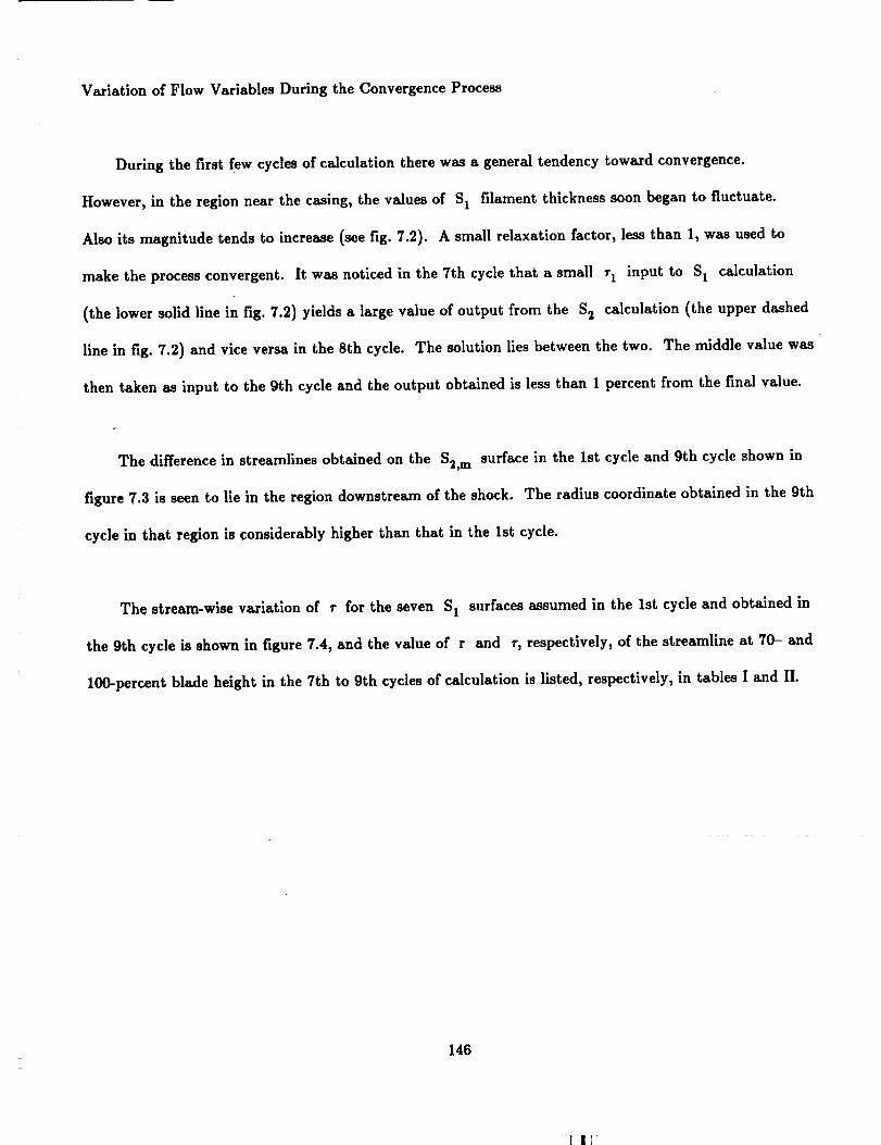
Variation of Flow Variables During the Convergence Process
During the first few cycles of calculation there was a general tendency toward convergence.
However, in the region near the casing, the values of S1 filament thickness soon began to fluctuate.
Also its magnitude tends to increase (see fig. 7.2). A small relaxation factor, less than 1, was used to
make the process convergent. It was noticed in the 7th cycle that a small r 1 input to S 1 calculation
(the lower solid line in fig. 7.2) yields a large value of output from the S2 calculation (the upper dashed
line in fig. 7.2) and vice versa in the 8th cycle. The solution lies between the two. The middle value was
then taken as input to the 9th cycle and the output obtained is less than 1 percent from the final value.
The difference in streamlines obtained on the $2, m surface in the 1st cycle and 9th cycle shown in
figure 7.3 is seen to lie in the region downstream of the shock. The radius coordinate obtained in the 9th
cycle in that region is considerably higher than that in the 1st cycle.
The stream-wise variation of r for the seven S 1 surfaces assumed in the 1st cycle and obtained in
the 9th cycle is shown in figure 7.4, and the value of r and r, respectively, of the streamline at 70- and
100-percent blade height in the 7th to 9th cycles of calculation is listed, respectively, in tables I and II.
146
1 |]

Z
o
i_ _
o
IP--4
• • °000
• •
O00
O00
O0 O
• o0 _ O
O00
• °00C
L",- _ 0
al
o
o
o
<
o
o
I
• ° o
• . °
• •
• , , , •
0 • , , • •
• • o
147

The converging process of V0r is similar to that of r of S1. The variation of V0r, relative to its
value at the exit, along the seven streamlines in the 9th cycle of calculation is compared to that in the 1st
cycle of calculation in figure 7.5.
On the other hand, the change in the angular thickness of stream filament $2, m is relatively simple.
The stream-wise value on the seven streamlines used as input value to the 9th cycle is shown in
figure 7.6(b) and is compared to those assumed in the 1st cycle (fig. 7.6(a)). The abrupt change in r
(and V0r streamline) is clearly seen in figure 7.5(b) (and 7.3(b), 7.4(b)).
Figure 7.7(a) shows the Mach number variation along the mean streamlines obtained on the seven
S 1 surfaces in the 9th cycle, whereas figure 7.7(b) shows those along the streamlines on the $2, m surface
obtained in the 9th cycle. They are very close; the maximum difference between the two being less than
4 percent. This is the same value previously obtained in the iteration for a subsonic rotor. This means
that in the present solution of moderately high transonic flow, the convergence and consistency level
obtained is as good as those in the subsonic case.
Three-Dimensional Flow Field
In the approximate three-dimensional solution presented herein, the three-dimensional flow field is
obtained on the seven S1 filaments of revolution extending over the whole blade passage (the $2, m
calculation is used mainly for obtaining the geometry of the S1 filaments). The constant Mach number
contours on these S1 surfaces can be readily obtained from the calculation. However, in order to make a
comparison to test data, the contours on S 1 surfaces at 18, 45, 68, and 89 percent span are obtained
through interpolation. They are shown in figures 7.8(a) to (d). They clearly show the strong effect of
the passage shock. The solution of S 1 surface flow can also be used to obtain the radial variation of
148

flow variablesat a numberof stationsalongtheflow direction.
andflow angle 3 are shown in figure 7.9.
Two of them, the relative Mach number
Although only the flow variation on the central S2 surface is directly available in the approximate
three-dimensional solution, those on the other S2 surfaces can be constructed by the data on the
corresponding streamlines on different S1 surfaces. Constant Mach number contours on the suction and
pressure surfaces are obtained in this way and are shown together with that on the central S_ surface in
figure 7.10. A second passage shock is seen on the suction surface and the central S2 surface, extending
only a short distant inward from the casing.
From data on these S2 surfaces, stream-wise variations of flow variables on certain streamlines can
be readily obtained. For instance, the variation of flow angle along three streamlines on the $2, m
surface at 18-, 68-, and 89-percent blade height (at inlet) are shown in figure 7.11.
The variation of flow variables can also be shown on spanwise surfaces formed by x _ and x 3
coordinates. The variations of M,/_, and p on these surfaces are particularly useful for observing the
influence of the passage shock and the magnitude of vorticity or secondary flow. Mach number contours
on three such surfaces are shown in figure 7.12. On the 10-percent chord surface, the intersection of
shock surface and this surface is seen to extend from the casing all the way inward to a point very near
the hub. At the 90-percent chord surface, the flow is almost entirely subsonic.
In order to more clearly see the effect of the three-dimensional passage shock on the three-
dimensional flow field, the three-dimensional passage shock is constructed in scale and is shown in
figure 7.13. At the tip Mach number of 1.37 and hub tip ratio of 0.5 the passage shock extends from
casing all the way inward almost to the hub.
149

Comparison Between Computed Flow Field with DFVLR Measured Data
The quasi-three-dimensional transonic solution obtained by the present method is compared with
available DFVLR measured data in figures 7.8, 7.9 and 7.11.
The character of the flow field obtained by the present method is seen to be in good agreement with
that constructed fromDFVLR measured data. In the region near 18-percent span, a supersonic zone
appears near the leading edge of the suction surface. In the middle of the span, a bow wave appears a
short distance in front of the leading edge and the wave extends to the flow passage to form a passage
shock. At about two-thirds of the span, the shock appears to be nearly attached to the leading edge.
Located in the blade tip region, is a second shock downstream of the bow wave/passage shock and the
shock is nearly normal to the suction surface. The position of the passage shock obtained in the
calculation is slightly in front of the measured position. It seems that this difference is inherent in the
solution of transonic flow by the use of the stream function/artlficial density method (refs. 41, 42, and
79). Also the computed shock is more nearly normal to the suction surface, whereas the measured shock
is more inclined to the suction surface.
The result calculated by a different method (ref. 34) is included in figure 7.8 for comparison. The
character of flow is similar, but there is some difference in the magnitude between the two calculated
results.
The relativelygood agreement between the calculatedand measured valuesofMach number and
flow angle in the radialdirection(fig.7.9)and flow anglealong the stream-wisedirection(fig.7.11)
indicatethat flowfieldin the centralportionof the three-dimensionalpassage determined in the present
method issufficientlyaccurateforengineeringcomputation. Itseems that a more accuratedetermination
of the shock position,such as the separatecalculation/shockfittingmethod (section6.1),appropriate
correctionforblockage effectat higherradius(section6.3,)and without assuming axiallysymmetrical SI
stream surfacemay improve the solutions.
150

7.2 Full-Three-Dimensional Transonic Flow in Cas Rotor
Solution Obtained by Using a Number of S1 and S2 Stream Filaments
The method described in Chapter 5 for obtaining three-dimensional flow using a number of S 1 and
S2 stream filaments was employed in reference 96 for calculating full-three-dimensional transonic flow in
the CAS rotor. A full-three-dimensional calculation was made after a quasi-three-dimensional solution
was been obtained. Thus, full-three-dimensional calculation can be used as a full-three-dimensional
analysis solution after the rotor is designed by the quasi-three-dimensional procedure.
The design parameters of the CAS compressor and details of testing were given in section 5.9. The
meridional projection of the rotor blades, design streamlines, L2F measuring stations, and the overall
performance of the rotor were given in figures 5.42 and 5.43. The radial distribution of stagnation
pressure and absolute flow angle measured by optical and non-optical devices are shown in figure 5.44.
Three-dimensional flow calculation has been carried out for 80 and 90 percent of design speed and
compared to the L2F data available at these two speeds.
Quasi-Three-Dimensional Solution for Transonic Flow in CAS Rotor
Quasi-three-dimensional solutions of transonic rotor were obtained for 80- and 90-percent design
speed. The stagnation pressure and the absolute flow angle, measured by Setra capacitance transistor
and L2F velocimeter, respectively, are taken as the outlet boundary conditions. The other main input
data are: flow path in meridional plane, blade geometry (coordinates given on S 1 surface or on
manufacturing templates), inlet pressure and temperature, rotor speed, mass flow and mass flow
coefficient.
151

The first step is to solve the flow along an $2, m surface about midway between two adjacent
blades. The computer code of reference 64, with a given absolute outlet flow angle and rotor efficiency, is
used for this purpose. The isentroplc efficiency of the rotor is determined by the torque measurement.
The radial distribution of rotor efficiency is calculated with the stagnation pressure and temperature
measurements. With the absolute velocity and flow angle measured by L2F velocimeter, the angular
momentum V0r is calculated. During calculation, the outlet flow angle a and radial distribution of
efficiency _s are updated successively, until V0r converges, and the calculated pressure p0 is in
agreement with the experimental values. This process takes only three to five cycles. The set of radial
distribution values of p0 a, and V0r at the outlet station and the rotor efficiency qs are used for
three-dimensional calculation of internal flow field and are compared with the L2F measured internal
flow field. Figure 7.14 shows the calculated values as compared to the measured values at the outlet
station.
From this solution of $2, m flow, the geometry of the 11 S1 surfaces of revolution and the variation of
the S1 stream filaments are obtained. The coordinates of the corresponding blade surface are calculated
by interpolation. The computer code of reference 41 is used to calculate the S 1 transonic flow. After
the solution of the flow on the 11 S 1 surfaces are obtained, a new $2, m surface along with the
corresponding variations of thickness of the S 1 filament Number 10 in figure 7.15. The angular
momentum V0r along streamline. Number 2 and Number 10 on the $2, m surface during iteration are
shown in figure 7.16. In figure 7.17 the relative Mach numbers along the intersecting streamlines
obtained on Si surface and on $2, m surface are shown. The closeness between the values shows the
degree of consistency as well as convergence reached in the solution.
Table III below gives the geometry and major flow parameters on six S1 stream filaments obtained
in the solution
152

11
9
7
5
3
1
M
TABLE III.--MAJOR PARAMETERS ON SIX S I
_1, #2, Coordinates r,mdegree degree
1.180 -66.2
1.089 -64.2
.993 -61.3
.883 -57.4
.758 -51.2
.609 -38.7
%o = 1.141 cm.
-56.2
-51.2
-45.7
-38.5
-27.6
3.8
_=0 _=.5
.3426 .3390
.3133 .3102
.2807 .2801
.2434 .2460
.1986 .2055
.1370 .1499
STREAM FILAMENTS OF REVOLUTION
f'_ f'o i
r1,0
"_=1
.3354
.3078
.2788
.2465
.2096
.1628
_'= 0 "_'= .s
1.000 1.014
1.092 1.021
1.234 1.121
1.404 1.305
1.730 1.589
2.638 2.461
_'=1 ro
.943 .943
.979 .896
1.071 .868
1.206 .859
1.433 .929
1.929 .731
O'p
degree
-7.98
- 5.49
-1.73
2.61
8.62
18.41
In the tablevaluesof ro,r0.s,rl, and r/ro show clearlythe quasi-three-dimensionalassumption of
the -S1 stream surface.Although the S1 surfaceisaxially-symmetric,the flow on SI variesinthe
circumferentialdirection.
The meridionalprojectionofstreamlineson $2,m isshown in figure7.18(a).
The stream-wlse variation of the S2 filament thickness and the angular momentum V0r at the mean
streamline on six S1 stream surfaces is shown in figures 7.19 and 7.20, respectively. On the S1 surface
near the hub, the flow is subsonic and these curves resemble those previously obtained in the subsonic
compressor (for example, fig. 5.40 and 5.39). But for the S 1 surface located in the region where a
passage shock exists, the curves are greatly affected by the shock.
The circumferential variations of relative Mach number at six axial stations on five S1 surfaces are
shown in figure 7.21.
153
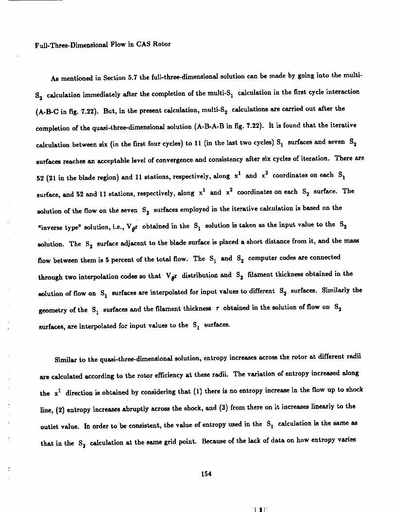
Full-Three-Dimensional Flow in CAS Rotor
As mentioned in Section 5.7 the full-three-dimensional solution can be made by going into the multi-
S2 calculation immediately after the completion of the multi-S 1 calculation in the first cycle interaction
(A-B-C in fig. 7.22). But, in the present calculation, multi-S 2 calculations are carried out after the
completion of the quasi-three-dimensional solution (A-B-A-B in fig. 7.22). It is found that the iterative
calculation between six (in the first four cycles) to 11 (in the last two cycles) S 1 surfaces and seven S_
surfaces reaches an acceptable level of convergence and consistency after six cycles of iteration. There are
52 (21 in the blade region) and 11 stations, respectively, along x I and x 2 coordinates on each S 1
surface, and 52 and 11 stations, respectively, along x I and x 2 coordinates on each S2 surface. The
solution of the flow on the seven S2 surfaces employed in the iterative calculation is based on the
_inverse type _ solution, i.e., V0r obtained in the S 1 solution is taken as the input value to the S2
solution. The S2 surface adjacent to the blade surface is placed a short distance from it, and the mass
flow between them is 5 percent of the total flow. The S 1 and
through two interpolation codes so that V#r distribution and
S2 computer codes are connected
S2 filament thickness obtained in the
solution of flow on S 1 surfaces are interpolated for input values to different Sz surfaces. Similarly the
geometry of the S1 surfaces and the filament thickness r obtained in the solution of flow on S2
surfaces, are interpolated for input values to the S1 surfaces.
Similar to the quasi-three-dimensional solution, entropy increases across the rotor at different radii
are calculated according to the rotor efficiency at these radii. The variation of entropy increased along
the x 1 direction is obtained by considering that (1) there is no entropy increase in the flow up to shock
line, (2) entropy increases abruptly across the shock, and (3) from there on it increases linearly to the
outlet value. In order to be consistent, the value of entropy used in the S 1 calculation is the same as
that in the S2 calculation at the same grid point. Because of the lack of data on how entropy varies
154

from blade to blade, the circumferential variation of entropy is considered neither on the
on different S2 surfaces.
S 1 surface nor
Converging Process
Since the main difference between a quasi-three-dimensional and a full-three-dimensional solution is
whether the radius of the S 1 surface is or is not circumferentially constant, the convergence in the
geometry of S 1 surface is an indication of the convergence of the full-three-dimensional solution.
Table IV lists the changes in the radii of three S1 surfaces during iteration. The corresponding changes
in S 1 filament are listed in Table V.
S 1
TABLE IV.--CHANGES IN RADIUS (m) OF GENERAL S I SURFACES DURING ITERATION
S 2St&tion
cycle21
.3111
.3118
.3118
.2784
.2791
.2791
.2425
.2430
.2429
31
.3102
.3101
.3101
.2790
.2_4
.2_4
.2453
.2453
.2453
41
.3083
.3081
.2781
.2793
.2790
.2790
.2473
.2469
.2469
21
.3126
.3131
.3131
.2807
.2811
.2811
.2451
.2445
.2445
IV
31
.3102
.3108
.3108
.2806
.2804
.2805
.2476
.2468
.2467
41
.3077
.3082
.3082
.2792
.2794
.2794
.2481
.2476
.2476
21
.3127
.3137
.3137
.2814
.2823
.2823
.2471
.2466
.2465
VII
31
.3098
.3108
.3108
.2802
.2806
.2806
.2483
.2475
.2474
41
.3070
.3080
.3080
.2792
.2793
.2794
.2490
.2480
.2479
155

$1
TABLE V.--CRANGES IN FILAMENT THICKNESS (cm) OF GENERAL S I SURFACES
S IStation
cycle
7 1
5
6
5 I
5
6
ro = 1.41 cm.
21
1.143
1.128
1.126
1.189
1.201
1.202
1.388
1.366
1.387
31
1.054
1.054
1.052
1.131
1.136
1.138
1.328
1.298
1.299
41
.986
.986
.985
1.063
1.075
1.075
1.2:]9
1.213
1.213
21
1.096
1.084
1.084
1.174
1.190
1.200
1.388
1.401
1.402
IV
31
1.035
1.039
1.037
1.087
1.120
1.121
1.294
1.295
1.296
41
.982
.977
.977
1.033
1.062
1.062
1.201
1.204
1.204
21
1.087
1.061
1.062
1.127
1.166
1.167
1.373
1.374
1.375
VII
31
1.050
1.037
1.036
1.059
1.103
1.104
1.277
1.279
1.279
41
.987
.955
.955
.989
1.034
1.035
1.160
1.158
1.159
Convergence in the radius of the general
stream filament is clearly indicated in Tables IV and V.
The Mach numbers along intersecting lines between $2, m
figure 7.17(b).
S 1 stream surfaces and in the thickness of the general S1
surfaces and S 1 surfaces are shown in
In figure 7.23 the Mach numbers along intersecting streamlines between S1 surfaces and S2 surfaces in
this solution are shown. A comparison between figures 7.17(a) and 7.17(b) and figure 7.23 itself indicates
that much better convergence and consistency are achieved in the full-three-dlmenslonal solution than
that achieved in the quasi-three-dimensional solution.
Geometry of S 1 and S2 Stream Filaments
Data in tables VI and VII show that the radius of the S 1 surface increases in the circumferential
direction at the blade leading edge, and the difference decreases toward the blade trailing edge. On the
other hand, the filament thickness at the leading edge is larger near the pressure surface at large radius
and larger near the suction surface at small radius. The difference decreases toward the trailing edge.
156
-1 lJ:

This configuration of the S1 stream filaments is a combined result of the flow vorticity and the passage
shock. In subsonic flow the relative circumferential difference in the radius is found to be about
0.2 percent, but in transonic flow the maximum value is about 1.3 percent, an order of magnitude higher.
The geometry of the S2 stream filaments is given in table VIII.
TABLE VI.--COORDINATE r (m) OF S I STREAM SURFACES
S 1, S 2
station
17
21
25
33
41
45
Number = 7
I II' III IV V
.2792 .2802 .2806 .2811 .2815
.2792 .2800 .2811 .2820 .2825
.2792 .2800 .2806 .2812 .2819
.2795 .2802 .2803 .2804 .2802
.2789 .2793 .2793 .2793 .2794
.2784 .2785 .2785 .2785 .2787
Number = 4
I II III IV V
.2201 .2205 .2214 .2222 .2229
.2229 .2230 .2239 .2248 .2259
.2243 .2248 .2256 .2263 .2268
.2271 .2278 .2284 .2287 .2290
.2294 .2299 .2301 .2303 .2307
.2304 .2305 .2306 .2305 .2308
TABLE VII.--THICKNESS OF S I STREAM FILAMENTS (r/to), r _,.
S v S 2
station
16
21
31
41
46
Number
I II
1.026 1.017
1.054 1.043
1.028 .986
.954 .946
.929 .928
11 (Filament of Revolution)
III IV V
1.008 1.001 .995
1.021 1.007 .996
.970 1.957 .957
.954 .957 .968
.929 .929 .928
Number 4 (General Filament)
I
1.251
1.202
1.138
1.075
1.042
I II III IV V I
16 1.643 1.653 1.653 1.652 1.647 3.49721 1.502 1.533 1.546 1.557 1.543 2.876
31 1.418 1.431 1.430 1.429 1.121 2.613
41 1.317 1.316 1.316 1.306 1.297 1.962
46 1.255 1.256 1.255 1.254 1.251 1.692
ro = 1.41 cm.
Number 7 (General Filament)
II III IV V
1.262 1.253 1.246 1.239
1.209 1.200 1.187 1.167
1.130 1.121 1.114 1.104
1.067 1.062 1.058 1.052
1.039 1.038 1.037 1.035
Number 1 (Filament of Revolution)
II III IV V
3.488 3.542 3.592 3.695
2.872 2.955 3.053 3.172
2.603 2.662 2.709 2.738
2.055 2.099 2.133 2.191
1.703 1.711 1.720 1.741
Figures 7.24 and 7.25 show, respectively, the 10 S1 stream filaments formed by the 11 S 1 stream
surfaces and the intersecting lines of the 11 S 1 stream surfaces with three span-wise surfaces. It is found
during calculation that the twist of the S 1 surface in the radial direction is relatively large at the blade
leading edge and relatively small at blade trailing edge. For instance, the radii of S 1 surface Number 5
157

at the blade leading edge are, respectively. 0.2429 m at the pressure surface and 0.2465 m at the suction
surface, a difference of 0 to 0.0036 m or 1.48 percent, but at the trailing edge they are, respectively,
0.2469 and 0.2479, a difference of only 0.001 m or 0.4 percent.
The geometry of S1 stream surfaces is one of the most important three-dimensional flow variables.
The blade section is now operating inside this filament. The flow characteristics are greatly influenced by
the variation of filament thickness in stream-wise as well as in circumferential direction.
Three-Dimensional Flow Field
The three-dimensional geometry of the S 1 stream filaments, given in tables VI and VII, and the
blade sections lying in the filament determine the flow along these filaments and consequently the flow
over the whole channels (see fig. 5.27). The meridional projection of the streamlines obtained on the
Sz, m surface S 2 filament thickness and Vsr along the mean streamline on six S 1 stream surfaces are
given in figures 7.18(h), 7.19(b) and 7.20(b), respectively. The difference between the solution obtained
in the present full-three-dlmensional solution and the previous quasi-three-dimensional solution is quite
apparent. The major geometry and inlet and outlet flow conditions of the six S1 stream filaments are
listed in table VI in which
point of chord length and
contraction in r
a and b denote the two corners at the upstream station, e and f at mid-
c and d at the downstream station, rc/ra, rd/r b and r¢/ra, rd/T b are the
and filament thickness r, respectively, on the two sides.
The flow determined on the six S 1 filaments is shown in figure 7.26 in terms of constant Mach number
contours. They are drawn for flow fields including four stations upstream and three stations downstream
of the blade. The inlet Mach number varies from 0.6 at the hub to 1.25 at the tip. The supersonic
region begins to appear on surface (3). On surface (7) a bow wave appears and extends to the suction
158
'1 i I_

surface as a passage shock.
50-percent chord point.
On the tip surface (11) the passage shock hits the suction surface at about
159

I
• I" " I' •
• " I" " I°/
I I I
r
' " I"
I I
160

The geometryof the S2 stream filaments is given in table VIII. Similar to the S 1 stream
filaments, the three-dimensional geometry of the S2 stream filaments and the meridional wall shape
determine the flow along these filaments and consequently the flow over the whole channel (see fig. 5.29).
figure 7.27 shows the constant Mach number contours on the S2 filaments. Notice that, whereas in the
quasi-three-dimensional solution only flow on one S2 surface (the $2, m surface), which took part in the
iteration, is directly obtained in the solution, in full-three-dimensional solution the flow on all S2
surfaces, which took part in the iteration, are directly obtained in the solution. The circumferentially
uniform flow at the inlet station becomes nonuniform near the blade leading edge, where tip Mach
number varies from 1.18 on S2 (I) to 1.21 on S2 (VII). It becomes uniform again at three stations
downstream of the blade. From the pressure surface of one blade toward the suction surface of the
adjacent blade, the intersection line of the shock and the surface becomes longer and moves downstream.
The flow condition on S2 (I) and (VII) should be particularly useful in the investigation of boundary
layer flow along the blade surfaces.
Using data obtained from these two families of stream surfaces a three-dimensional view of the shock
can easily be constructed (fig. 7.28). The passage shock is seen to extend from the casing part way
(about two-thirds) down to the hub. The shock is nearly normal to the suction surface and more inclined
at lower radius.
Using data obtained on the S 1 and S2 surfaces, constant Mach number contours can also be
constructed on a number of a third family of surfaces, formed by the x 2 and x 3 coordinates, nearly
normal to S1 and S2 surfaces at stations 1 (L.E.), 5, 9, 11, and 21 (T.E) (fig. 7.28). In the stream-
wise direction the shock intersection line becomes shorter, and the circumferential gradient in Mach
number becomes smaller. Between station 11 and 21 appears a reverse circumferential Mach number
161

gradient in the lower part of the passage. Consequently there is also a reverse circumferential gradient in
pressure, which will affect the boundary layer along the hub wall.
Constant a contours are obtained on five such surfaces and are shown in figure 7.30. At station
J---0 (one station upstream of the blade) there is a significant difference circumferentially in the upper
half of the flow channel. At the pressure surface side ¢ is +2 °, whereas on the suction surface side, ¢
is -2 ° to -6 °. This difference in o means that the air is moving outward on the left and moving
inward on the right. At station 2 the air on the upper left is now moving inward with -8 ° to -10 °.
Thus there is a twist of S1 surface between station 0 and station 2. It is nearly uniform
clrcumferentially at station 6. At station 10 a sharp change of 2 ° appears in the flow direction over most
part of the channel. At station 21 the value ¢ is again nearly uniform in the circumferential direction.
The stream-wise variations of filament thickness and angular momentum V0r of S2 stream
filaments (I), (IV), and (VII) are shown, respectively, in figures 7.31 and 7.32. As for the filament
thickness r, the variation in the subsonic hub region is similar to that of (P-t)/P, except that there is a
high peak value at the leading edge on the S2(I ). In the supersonic upper region the variation of S2(I )
and S_(VII) are quite different from (P-t)/P. On S2(IV ) there is still some resemblance, but it has two
peaks around the leading edge, indicating the effects of bow wave and passage shock.
The variation of V0r is somewhat similar. In the hub region it is only slightly modified from the
usual shape in subsonic flow. But in the upper part there is quite a peak at leading edge near the
pressure surface and an overshoot at the trailing edge near the suction surface. In the tip region there is
either a two-step rise or fluctuation in the V0r variation.
162
-1 Iv

Difference Between Three-Dimensional and Quasi-Three-Dimensional Solution
The difference between three-dimensional and quasi-three-dimensional solution is entirely due to the
difference in the geometry of the S1 stream filament. Tables III and VIII show the major difference
between the S 1 stream filaments involved in the two calculations.
First, there is some difference in the geometry of $2,m in the radial coordinate and in the
contraction of the filaments thickness. Figure 7.19 shows the difference in the streamwise variation of the
$2, m filament thickness.
A rather complicated variation in the full-three-dimensional flow is much simplified in the quasi-
three-dimensional flow. The streamwise variations of the important flow variable Vor on the $2, m
surface are compared in figure 7.20. A higher overshoot exists in the quasi-three-dimensional solution.
The streamwise variations of Mach number along the intersecting streamline of the S 1 and S_, m
surfaces, obtained in the solution on the two surfaces, are compared in figure 7.17. The full-three-
dimensional solution has reached a higher level of consistency and convergence than the quasi-three-
dimensional solution. The former, in general, gives a slightly higher peak Mach number than the latter.
This difference is also noticeable in the comparison of the constant Mach number contour maps on the
$2, m surface shown in figure 7.34.
Circumferential variations of Mach number at six stations on five S 1 surfaces obtained in full-three-
dimensional and quasi-three-dimensional solution are compared in figure 7.21. In addition to the factors
influencing the solution mentioned above, the circumferential variation in the S 1 geometry in the full-
three-dimensional solution also influences the result. It can be seen from tables V, VI, and VIII that for
S 1 surfaces above $1(7), the filament thickness and its contraction on the side near the pressure surface
163

issignificantlydifferentfrom thoseon the side near the suction surface. The combined effect on the
velocity distribution is that, on S1 surfaces above $I(7), the Mach number of the full-three-dimensional
solution is higher in the region from mid-channel to suction surface and lower in the region from mid-
channel to pressure surface, than that of the quasi-three-dimensional solution.
Comparison with L2F Measurement
Efforts were made at IETP to obtain internal flow on S1 surface (4), and (7) to (I0) by the use of
a Laser-2-Focus (L2F) velocimeter developed by DFVLR. Measured values are shown in figure 7.21. In
general the measured values are a little higher than the calculated values. Constant Mach number
contours, constructed from the L2F measured data, are shown in figure 7.33. The trend is similar, but
again the measured Mach number is a little higher than the calculated value.
7.3 Some Remarks
The general theory of three-dimensional flow in subsonic and supersonic turbomachinery based on
the iterative solution between S1 and S2 stream filaments has been successfully extended to a transonic
flow regime. In this extension, some of the recently developed simple and quick methods for solving
transonic flow along S1 and S2 stream filaments are utilized. For the CAS transonic rotor, three-
dimensional solution is obtained after six cycles of iteration by using the quasi-three-dimensional solution
as the starting value. It has a higher level of convergence and consistency than the quasi-three-
dimensional solution. The difference between three-dimensional and quasi-three-dimensional solution is:
The former gives a higher peak Mach number than the latter. This difference is mainly due to the
neglect of the circumferential variation of the S1 filament thickness in the quasi-three-dimensional
solution. A comparison between the theoretical solution and the L2F measurement shows that the
164
characterof thetransonicflow includingthe three-dimensionaishockstructureis in fair agreement,and
the calculatedvelocityis a little lower than that measured by L2F over most of the flow region, except
at the 20-percent chord station in the upper half region near the suction surface, where the measured
velocity is a little lower.
A practical three-dimensionai computer aided design and analysis (three-dimensional-CADA) system
has been constructed by the use of the general S1 code and the general S2 code. The recommended
procedure of three-dimensional-CADA calculation follows.
(1) Prescribed the through-flow design requirements on the $2, m
solution
(2) Design the blade section on a number of general S1
(3) Stack the blade sections
(4) Obtain the three-dimensional analysis for the blade just designed
surface and obtain the $2, m
stream filaments
(5) Modify step 1 or step 2 and repeat steps 3 and 4 until the results obtained meet the design
requirements
It is believed that the configuration of the three-dimensional geometry of the S 1 stream filaments,
obtained during the iterative calculation between the S 1 and S2 flow, to a large extent, determines the
performance of the blade section lying in the stream filament. With this information available better
design of the blade section and, consequently, of the whole blade can be realized. Another advantage of
the presented method is that the computer storage required is very small and the amount of CPU time is
also small so it is feasible to carry out all of the computations on a microcomputer.
165

References
1. Wu, Chung-Huaand Wolfenstein, L.: "Application of Radial-Equilibrium-Condition to Axial-Flow
Compressor and Turbine Design," NACA TR 955, 1950.
2. Wu, Chung-Hua: "A General Through-Flow Theory of Fluid Flow with Subsonic or Supersonic
Velocity in Turbomachines Having Arbitrary Hub and Casing Shapes," NACA TN 2302, 1951.
3. Wu, Chung-Hua: _A General Theory of Three-Dimensional Flow in Subsonic and Supersonic
Turbomachines of Axial,Radial,and Mixed-Flow Types," ASME Paper Number 50-A-79,ASME
Transactions,November 1952, or NACA TN 2604, 1952.
4. Wu, Chung-Hua and Brown, C.A.: UMethod of AnalysisforCompressible Flow Past Arbitrary
Turbomachine Blades on General Surfaceof Revolution,"NACA TN 2407, 1951.
5. Wu, Chung-Hua and Brown, C.A.: "A Method of DesigningTurbomachine Blades with a
DesirableThickness DistributionforCompressible Flow along an ArbitraryStream Filament of
Revolution,"NACA TN 2455, 1951.
6. Wu, Chung-Hua and Brown, C.A.: _An Approximate Method ofDetermining the Subsonic Flow in
an ArbitraryStream Filament ofRevolution Cut by ArbitraryTurbomachine Blades,_ NACA
TN 2702, 1952.
7. Wu, Chung-Hua and Curtis,A. et al.:"Analysisof Flow in a Subsonic Mixed Flow Impeller,"
NACA TN 2749, 1952.
8. Prian,V.D., Kramer, J.,and Wu, C.H.: "TheoreticalAnalysisof IncompressibleFlow Through a
Radial-lnletCentrifugalImpellerat Various Weight Flows. I. Solutionby a Matrix Method and
Comparison with An Approximate Method," NACA TN 3448, 1955.
9. Wu, Chung-Hua and Costilow,Eleanor,L.: "A Method of Solvingthe Directand InverseProblem
of SupersonicFlow Along ArbitraryStream Filamentsof Revolution in Turbomachines,_ NACA
TN 2492, 1951.
166

10. Wu, Chung-Hua: "Matrix and Relaxation Solutions that Determine Subsonic Through-Flow in an
Axial-Flow Gas Turbine," NACA TN 2750, 1952.
11. Wu, Chung-Hua: "Subsonic Flow of Air Through a Single-Stage and a Seven Stage Compressor:
NACA TN 2961, 1953.
12. Marsh, H.: "A Digital Computer Program for the Through-Flow Fluid Mechanics in an Arbitrary
Turbomachine Using a Matrix Method," R&M Number 3509, 1968.
13. Katsanis, T.: "Computer Program for Calculating Velocities and Streamlines on a Blade-to-Blade
Stream Surface of a Turbomachine," NASA TN D-4525, 1968.
14. Katsanis, T. and McNally, W.D.: "Fortran Program for Calculating Velocities and Streamlines in
a Magnified Region on a Blade-to-Blade Stream Surface of a Tandem Turbomachine," NASA TN
D-5044, 1969.
15. Senoo, Y. and Nakase, YI: "A Blade Theory of an Impeller with an Arbitrary Surface of
Revolution," ASME Journal of Engineering For Power, vol. 93, 1971, pp. 454-460.
16. Davis, W.R.: "Axial Flow Compressor Analysis Using a Matrix Method," Carleton University,
Report Number MW/A 73-1, 1973.
17. Smith, D.J.L.: "Computer Solutions of Wu's Equations for the Compressible Flow through
Turbomachines," in NASA SP-304, 1973.
18. Katsanis, T., and McNally, W.D.: "Fortran Program for Calculating Velocity and Streamlines on
the Hub-Shroud Mid-Channel Flow Surface of an Axial- or Mixed-Flow Turbomachine," NASA TN
D-7343, 1973.
19. Adler, D. and Krimerman, Y.: "The Numerical Calculation of the Me ridional Flow Field in
Turbomachines Using the Finite Elements Method," Israel Journal of Technology, vol. 12, 1974,
pp. 268-274.
20. Hirsch, Ch., and Warzee, G.: "A Finite Element Method for Through Flow Calculation in
Turbomachines," Journal of Fluids Engineering, vol. 98, 1976, p. 403.
167

21. Bianiaris,S.: "The CalculationofQuasi-Three-DimensionalFlow in the Axial Gas Turbine,"
ASME Journalof EngineeringforPower, pp. 283-294, 1975.
22. Adler,D. and Krimerman, Y.: "Calculationofthe Blade-to-BladeCompressible Flow Fieldin
Turbo ImpellersUsing FiniteElement Method, _ JournalofMechanical EngineeringScience,vol.
19, 1978,pp. 108-112.
23. Senoo,Y. and Nakase, Y.: "An AnalysisofFlow Through a Mixed-Flow Impeller,_ Journal
ofEngineeringfor Power, vol.94, 1972,pp. 43-40.
24. Bosman C. and EI-Shaaraw,M.A.I.: "Quasi-Three-DimensionalNumerical Solutionof Flow in
Turbomachines," Journalof FluidsEngineering,vol.99, 1977,pp. 132-140.
25. Hirsch,Ch. and Qarzee, G.: "An IntegratedQuasi-Three-DimensionalFiniteElement Calculation
Program forTurbomachlnery Flows," Journal ofEngineeringforPower, vol.101,1979,pp.
141-148.
26. Krimerman, Y. and Adler,D.: "The Complete Three-Dimensional Calculationofthe Compressible
Flow Fieldin Turbo-lmpellers,_ Journal ofMechanical EngineeringScience,vol.20, 1978,
pp. 149-158.
27. Wu, Chung-Hau: Formulas and Tables of CoefficientsforNumerical Differentiationwith Function
28.
Values Given at Unequally Spaced Points and Applicationto the Solutionof PartialDifferential
Equations,SciencePress,1959.
Wu, Chung-Hua: "BasicAerothermodynamic Equations Governing Fluid Flow in
Turbomachines Expressed inTerms of Non-Orthogonal CurvilinearCoordinates,_ Research
Notes,InstituteofMechanics, C.A.S.,1963.
168
I II

29. Wu, Chung-Hua: "Three-Dimensional Turbomachine Flow Equations Expressed with Respect to
Non-orthogonal Curvilinear Coordinates and Methods of Solution," Lecture Notes, China
University of Science and Technology, 1975 or "Proceedings of the 3rd International Symposium on
Air-Breathing Engines," 1976, pp. 233-252, or Engineering Thermophysics in China, vol. 1, no. 2,
1980, Rumford Publishing Company, USA.
30. Luu, T.S., Viney, B. and Corniglion, J.: "Conception optimale de l'alimentation latdrale d'une
turbomachine," AAAF 18e Colloque Adrodynamique Appliqude, Poitiers 1981.
31. Zhu, G.X., and Wu, C.H.: "Three-Dimensional Subsonic Flow Through a Stator by Use of a
Central S2 Stream Surface and Several S1 Surfaces of Revolution," Journal of Engineering
Thermophysics, vol. 4, no. 2, pp. 134-142, 1983. (in Chinese).
32. Wang, Qinghuan, Wu, Wenquan, Zhu, Genxing, Li, Weihong and Wu, Chung-hua: "Solution of
Three-Dimensional Compressible Flow in an Axial-Flow Compressor Stator by the Use of S1 and S2
Relative Surface, _ Journal of Engineering Thermophysics, vol. 4, pp. 336-346, 1983, (in Chinese).
33. Wu, Chung-Hua, Wang, Jianan, Fang, Zongyi, and Wang, Qinghuan: "L2F Velocity
Measurement and Calculation of Three-Dimensional Flow in an Axial Compressor Rotor, _
Proceedings of 7th ISABE, 1985.
34. McDonald, R.W.: "The Computation of Transonic Flow Through Two-Dimensional Gas Turbine
Cascades," ASME Paper 71-GT-89, 1971.
35. Gopalakrishnan, S., and Bozzola, R.: "A Numerical Technique for the Calculation of Transonic
Flows in Turbomachinery Cascades," ASME Paper No. 71-GT-42, 1971.
36. Denton, J.D.: "A Time Marching Method for Two- and Three-Dimensional Blade-to-Blade Flows, _
Aeronautical Research Council, 35567, 1974.
37. Wu, C.H., Wu, W., Hua, Y., and Wang, B.: gTransonic Cascade Flow with Given Shock Shape
Solved by Separate Supersonic and Subsonic Computations," Computational Methods in
Turbomachinery, I Mech E, Paper No. C19/84, pp. 133-140, 1984.
169

38. Wu, Wenquan,Wu,Chunghua,andYu, Dabang: "Transonic Cascade Flow Solved by
Separate Supersonic and Subsonic Computation with Shock Fitting," Jrl. of Engineering for
Gas Turbines and Power, Apr, 1985.
39 Qin, Lisen and Wu, Chung-Hua: "Transonic Flow along S2 Stream Surface Solved by Separate
Supersonic and Subsonic Calculations," ISABE Paper 85-7058, Proceedings of 7th International
Symposium for Air-Breathing Engines, pp. 502-509, 1985.
40. Habashi, W.G., Hafez, M.M.: "Finite Element Stream Function Solution for Transonic
Turbomachinery Flows," AIAA 82-1268.
41. Zhao, Xiaolu: "Solution of Transonic Flow along S 1 Stream Surface Employing Non-Orthogonal
Curvilinear Coordinates and Corresponding Non-Orthogona] Velocity Components," Journal of
Engineering Thermophyslcs, Aug. 1984, pp. 244-249 (in Chinese), or C64/84, Computation
Methods in Turbomachinery, I Mech E, pp. 183-189.
42. Wang, Zhengming: "Solution of Transonic S 1 Surface Flow by Successively Reversing the
Direction of Integration of the Stream Function Equation," Jrl. of Engineering Thermophysics,
Aug. 1984. (in Chinese), or Engineering for Power, Apr. 1985.
43. Wu, Chung-Hua: "Fundamental Aerothermodynamic Equations for Stationary and Moving
Coordinate Systems: Action of Viscous Forces and Physical Significance of Viscous Terms,"
Journal of Mechanical Engineering, vol. 13, no. 4, December 1965, pp. 43-67 (in Chinese) or
Engineering Thermophysics in China, vol. 1, no. 1, 1980, Rumford Publishing Company, USA.
44. Wu, Chung-Hua: Discussion to Paper "A Practical Solution of a Three-Dimensional Flow Problem
of Axial-Flow Turbomachinery, _ ASME Transactions, July 1953, pp. 802-803.
45. Vevra, M.H., .Aero-Thermodynamics and Flow in Turbomachines, 1960.
46. Sirotkin, Is, A.: "Formulation of Straight Problem of Vortex Flow of Compressed Fluid in
Turbomachines," Inzhenernyi Zhurnal, Journal of Engineering, vol. 3, no. 2, pp. 271-279, 1963.
170
_t l i-

47. Johnson, I.A., and Bullock, R.O.:
SP-36, 1965.
48. Chen, Hongji, and Wu, Chung-Hua:
"Aerodynamic Design of Axial-Flow Compressor, _ NACA,
"Accurate Solution of Inverse Problem of Transonic Flow on
S2 Surface by Means of Elliptic Algorithm. _ Proceedings of 7th ISABE, pp. 465-473, 1985.
49. Rahnke, C.J. and Carmody, R.H.: "The Combined Transonic Axial and Centrifugal Stage
Compressor, _ SAE Paper 268D, 1961.
50 Serovy, G.K.: "Recent Progress in Aerodynamic Design of Axial-Flow Compressor in the United
States, _ Journal of Engineering for Power, July, 1966.
51. Miller, M.L. and Chapman, D.C.: "Single-Stage Experimental Evaluation of Boundary Layer
Blowing Technique for High Lift Stator Blades, _ I--Compressor Design, NASA CR-54564, 1969.
52. Fujii, S., and Matsuki, M.: "Several Topics of Axial-Flow Compressor Research at The National
Aerospace Laboratory (Japan) _ Gas Turbine Papers presented at Tokyo Joint International Gas
Turbine Conference and Products Show, 1971.
53. Senoo, Y. and Nakase, Y.: "An Analysis of Flow Through a Mixed-Flow Impeller, _ Journal of
Engineering for Power, vol. 94, 1972, pp. 40-43.
54. Wu, Chung-Hua and Brown, C.A.: "A Theory of Direct and Inverse Problems of Compressible
Flow Past Cascade of Arbitrary Airfoils, Journal of Aeronautical Sciences, March, 1952.
55. Liu, Kao-Lien, Hsieh, Ming-Lun and Wu, Chung-Hau: "Aerothermodynamic Analysis and Design
of Turbomachines, _ Chinese Journal of Mechanical Engineering, March, . 11, No. 1, pp. 1-28, 1963.
56. Cai, R.: "The Analytical Solution for MSLM for 2D Cascade, _ Journal of Mechanical Engineering,
(in Chinese), vol. 14, no. 1, 1966, pp. 17-49 .....
57. Cai, R.: "A Method of Designing Axial F10w Turbomachine Cascades Along an Arbitrary Stream
Filament of Revolution, _ Journal of Mechanical Engineering, (in Chinese), vol. 15, no. 1, 1979,
pp. 24-36.
171

58. Wang,Z. and Cai, R.: "MSLM with Higher-Order Derivatives and the Computer Code, s Journal
of Engineering Thermophysics, (in Chinese), November, 1983, pp. 347-350.
59. Zhao, X.: "A Method for Solving Inverse Problem of Three-Dimensional Turbomachine Flow--the
Mean Stream Surface Method, and the Annular Constraint Condition," M.S. Thesis, Institute of
Engineering Thermophysics, 1981 (in Chinese).
60. Sun, C.: "A New Method for Series Expansion from $2, m Surface," M.S. Thesis, Institute of
Engineering Thermophysics, 1983 (in Chinese).
61. Zhao, X., Sun, C. and Wu, Chung-Hua: "A Simple Method for Solving Three-Dimensional
Inverse Problems of Turbomachine Flow and the Annular Constraint Condition," Journal of
Engineering for Gas Turbines and Power, vol. 107, 1985, pp. 293-300.
62. Academia Sinica and Shengyang Aeroengine Company: "Theory, Methods and Application of
Three-Dimensional Flow Design of Transonic Axial-Flow Compressor, _ Journal of Engineering
Thermophysics, vol. 1, no. 1, 1980, pp. 44-54 (in Chinese).
63. Wu, W. and Liu, C.: "Flow-Field Matrix Solution for Direct Problem of Flow Along S1 Relative
Stream Surface Employing Non-orthogonal Velocity Components," Journal of Engineering
Thermophysics, vol. 1, no. 1, 1980, pp. 18-27 (in Chinese) or Engineering Thermophysics in China,
vol. 1, no. 3, pp. 307-322, Rumford Publishing Company, USA.
64. Zhu, R.: "Flow-Field Line Relaxation Solution for S 2 Relative Stream Employing Non-
Orthogonal Curvilinear Coordinates and Corresponding Non-Orthogonal Velocity Components, _
Journal of Engineering Thermophysics, vol. 2, no. 3, 1980.
65. W.W. and Jian, H.: "A Development in Calculation of Flow Past Cascade on Arbitrary Surface of
Revolution, _ C83/84. Computational Methods in Turbomachinery, I Mech. E, pp. 265-270, 1984.
66. Wu, Chung-Hua and Wang, Baoguo: "Matrix Solution of Compressible Flow on S1 Surface
Through a Turbomachine Blade Row with SplitterVanes or Tandem Blades,"ASME
Journalof EngineeringforGas Turbines and Power_ vol.106,April,1984,pp. 449-454.
172
I I i

67. Wang, Z.: "Inverse Design Calculations for Transonic Cascades," ASME Paper 85-GT-6, 1985.
68. Cai, Ruixian: "Constraint on Design Parameters and Twist of S1 Surfaces in Turbomachines, _
Scientia Sinica (Series A), Apr. 1983.
Liu, C.E., and Wu, W.Q.: _Computer Program of Supersonic Flow Past Inlet of Cascade Section
on an Arbitrary Stream Filament of Revolution and Determining Unique Inlet Flow Angle, _
Journal of Engineering Thermophysics, vol. 1, no. 3, 1980.
70. Moeckel, W.E.: "Approximate Method for Predicting Form and Location of Detached Shock
Waves Ahead of Plane or Axially Symmetric Bodies, _ NACA TN 1921, 1949.
71. Love, E.S.: "A Reexamination of the Use of Simple Concepts for Predicating the Shape and
Location of Detached Shock Waves, _ NACA TN 4170, Dec. 1957.
72. York, R.E., and Woodard, H.S.: "Flow in the Entrance Region of Supersonic Compressor
Cascades, _ ASME Journal of Engineering for Power, Apr. 1976, pp. 247-257.
73. Starken, H.: "Research of The Flow in a Plane Supersonic Diffuser Cascade," (in English) DLR
FB 71-99 DFVLR Institut fur Luftstrahlantriebe.
74. Ruan, Z.K.: "Experimental Determination of Shape and Location of Bow Shock Wave Ahead of a
Plane Cascade, _ Journal of Engineering Thermophysics, vol. 4, no. 4, pp. 338-341, 1983.
75. Hua, Yao-nan: "Computation of the Detached Shock and the Entrance Flow Field in a Supersonic
or Transonic Cascade," ASME 85-GT-7.
76. Hoist, T., Ballhaus, W.: "Fast Conservative Schemes for Full Potential Equation Applied to
Transonic Flows," AIAA J. 1979, 17, pp. 145-152.
77. Hafez, M.M., South, J., and Murman, E.M.: "Artificial Compressibility Methods for Numerical
Solution of Transonic Full Potential Equation, _ AIAA Journal, vol. 17, no. 8, 1979.
78. Hafe,., M., Lovell, D.: "Numerical Solution of Transonic Stream Function Equation, AIAA 81-
1017.
173

79. Hua,Y., Wu, W.: "NumericalSolution of Transonic Stream Function Equation on S 1 Stream
Surface in Cascade, _ ASME 86-GT-110, 1986.
80. Roach, R., Sankar, N.: "The Strongly Implicit Procedure Applied to the Flow Fluid of Transonic
Turbine Cascade, _ AIAA 81-0211, 1981.
81. Stone, L.: "Iterative Solution of Implicit Approximations of Multi-Dimensional Partial
Differential Equations, z SIAM J. of Numerical Anallsis, 1968, vol. 3, 530-558.
82. Dunavant, J. and Erwin, J.: "Investigation of a Related Series of Turbine-Blade Profiles in
Cascade_ z NACA TN 3892, 1955.
83. Dodge, P.: "Transonic Relaxation Methods, _ ASME Paper 76-GT-63, 1976.
84. Lu, W.Q., Chen, X.M.: "The Time-Dependent Numerical Solution of Transonic Flow on S 1
Surface of Revolution Employing Non-Orthogonal Curvilinear Coordinates and Non-Orthogonal
Velocity Components, z J. of Engineering Thermophysics (in Chinese), 1983, 4, pp. 119-126.
85. Wang, B., Hua, Y., I-Iuang, X., Wu, C.H.: "Transonic Flow Along Arbitrary Stream Filament of
Revolution Solved by Separate Computations with Shock Fitting, z ASME Paper 86-GT-30, 1986.
86. Zhao Xiaolu, Qin Lisen: "Stream Function Solution of Transonic General S1 Flow in
Turbomachines, J. of Eng. Thermophysics, vol. 8, no. 4, pp. 340-342 (in Chinese), 1987.
87. Monsarrat, N.T. et al.: Design Report. Single-Stage Evaluation of Highly-Loaded High Mach-
Number Compressor Stages, NASA CR-72562, 1969.
88. Chen Hongji and Wu Chunghua: "Shock Embedding Discontinuous Solution of Elliptic Equation
for Inverse problem of Transonic S2 Flow, z ASME Paper No. 87-GT-115, Journal of
Turbomachinery, vol. 110, pp. 347-353, 1988.
89. Strinning, P.E., Dunker, R.J.: "Aerodynamic and Blade Design of a Transonic Axlal-Compressor
Stage, _ Forsungsberichte Verbrennungs-Kraftmachines, Heft 178, 1975.
174
_TIF

90. Dunker, R.J., Strinning, P.E.: "Flow Velocity Measurements Inside of a Transonic Axial
Compressor Rotor by Means of an Optical Technique and Compared with Blade to Blade
Calculations, _ 3rd ISABE Proceedings, DGLR-Fachbuch No. 6, March, 1976.
91. Zhao Xiaolu: "Stream Function Solution of Transonic Flow Along S2 Streamsurface of Axial
Turbomachines,: ASME Paper 85-GT-2, 1985.
92. Zhao Xiaolu: "Transonic Stream Function Solution on S2 Streamsurface for a High Pressure
Ratio Centrifugal Compressor," Journal of Engineering Thermophysics, vol. 9, no. 1 (in chinese),
1988.
93. Asborne, C., Runstadler, P.W., Stacy, W.D.: "Aerodynamic and Mechanical Design of an 8:1
Pressure Ratio Centrifugal Compressor, _ NASA CR-134782, 1975.
94. Hayami, H., Senoo, R., Veki, H.: "Flow in the Inducer of a Centrifugal Compressor Measured with
a Laser Velocimeter, _ ASME 84-GT-74, 1984.
95. Wang Zhengming, Chen Hongji, Hua Yaonan, and Wu Chung-Hua: "Solut;on of Transonic Flow
in an Axial Compressor Rotor by Quasi-3D Iteration Between S1 and S2 Stream Surface, _
Chinese Journal of Engineering Thermophysics, vol. 1, no. 2, pp. 153-166, 1989.
96. Zhao Xiaolu, Qin Lisen and Wu Chung-Hua: "A Quasi-3D Computation for the CAS Transonic
Compressor Rotor and Comparison with L2F Velocity Measurements, _ Chinese Journal of
Engineering Thermophysics, vol. 1, no. 1, 1989, pp. 29-37.
97. Zhao Xiaolu, Qin Lisen and Wu Chung-Hua: "A Full-3D Iterative Solution on S1 - S_ Stream
Surfaces in the CAS Transonic Compressor Rotor, _ Chinese Journal of Engineering Thermophysics,
vol. 1, no. 4, 1989, pp. 391-400.
98. Qin Lisen, Zhao Xiaolu and Wu Chung-Hua: "Analysis of FuII-3D S1--S 2 Iterative Solution for
Flow in the CAS Transonic Compressor Rotor and Comparison with Quasi-3D Iterative Solution
and L2F Measurement," Chinese Journal of Engineering Thermophysics, vol. 2, no. 1, 1990,
pp. 29-38.
175

99.
100.
Wu Chunghua,WangZhengming,ChenHongji: "Three-DimensionalRotational Flow in Transonic
Turbomachines, Part I--Solution Obtained by Using a Number of S 1 Stream Filaments of
Revolution and a Central S2 Stream Filament," ASME Paper 90-GT-12, J. of Turbomachinery,
vol. 114, no. 1, pp. 38-49.
Wu Chunghua, Zhao Xiaolu, Qin Lisen: _3D Rotational Flow in Transonic Turbomachines, Part
II--Full Three-Dimensional Flow in CAS Rotor Obtained by Using a Number of S 1 and S 2
Stream Filaments, _ ASME Paper 90-GT-13, J. of Turbomachinery, vol. 114, no. 1, pp. 50-60.
176

By
Figure 2.1 .--Stress tensor.
/////,
v,j• el.r
V 'r+ _ 8y
_j _" i÷ r'-¥-t i .--_6v i..e- [ _,- ._
j __1_i_x___
_'/////////////////////, //_,//
T1
Figure 2.2.--Velocity and temperature profile and fluid element in a laminar boundary layer.
...=...,.=
=--I1_
r
A
f,.,,..--
.,....,.=--,.---'3
,-U
V_,
Inlet guide vanes Rotor Stator
Figure 2.3---Relative stream surface in inlet guide vanes, rotorand stator.
177

1.0
0.8
r*
0.6
O.4-0.2
_e
i1 r" 0.4
0.2=
mm_m_m=m
I I I I [ I I I I L0 0.2 0.4 0.6 0,8 1.0 1.2 1.4 1.6 1.8
Z °
Figure 2.4--Projection of streamlines in meridional plane.
////_
_=_=-.-'_" X or
Figure 2.5,--Radial variation of rotor effickmcy,entropy increase and velocity.
t78
I2.0

Figure 3,1 mRelatlve stream surface S 1.
z
Rgure 3.2--Relative stream surface S 2.
179

/2r
Figure 3.3.--Intersecting S 1 and S 2 surfaces in blade passage.
q+
dz
_z
Dz
$2 q, dr
$2 q÷
¢p
Figure 3.4.--Partial derivative and total derivative following motion on S 2.
180
=_lIll

S2m
• /-- T + _r dr + _'dz
_wr÷_Wr_drT
/ I _ T OZdr "
ooooo°°"
r pWr j,
dz j + r(&_)
Figure 3.5.--Element of S 2 stream filament. Figure 3.6---S 2 stream surface and S 2 stream filament.
dr
dz
Figure 3.7.--Orthogonal curvilinear coordinates e, _, on S t surface of revolution.
181
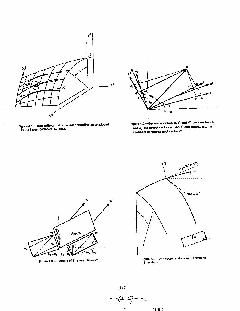
y2
y3
/
Figure 4.1 .--Non-orthogonal curvilinear coordinates employed
in the Investigation of S 1 flow.
I W
e2 e2 I
I 81 e 2
Figure 4.2.--Genend coordinates x1 and x;_, base veclom e 1
and e2, reciproca/vectors e1 and e2 and contrm/ahant and
covariant components of vector W,
W W
W 2 W_ w
Figure 4.3.--Element of S 1 stream filament, Figure 4.4.--Unit vector and vorticity normal to
S 1 surface.
182
1 I I

y2
X 2
J y1
y3
Figure 4.5.--Non-orthogonal curvilinear coordinates used for
S 2 flow.
;)X2
DqDt
q + _1 dx 2ax2
\dx 1
I
_o
Figure 4.6.--Partial derivative and total derivative following fluid flow on S 2 surface.
183

x2
x1
Figure 4.7.--Line integration around grid point E.
184
l ! l
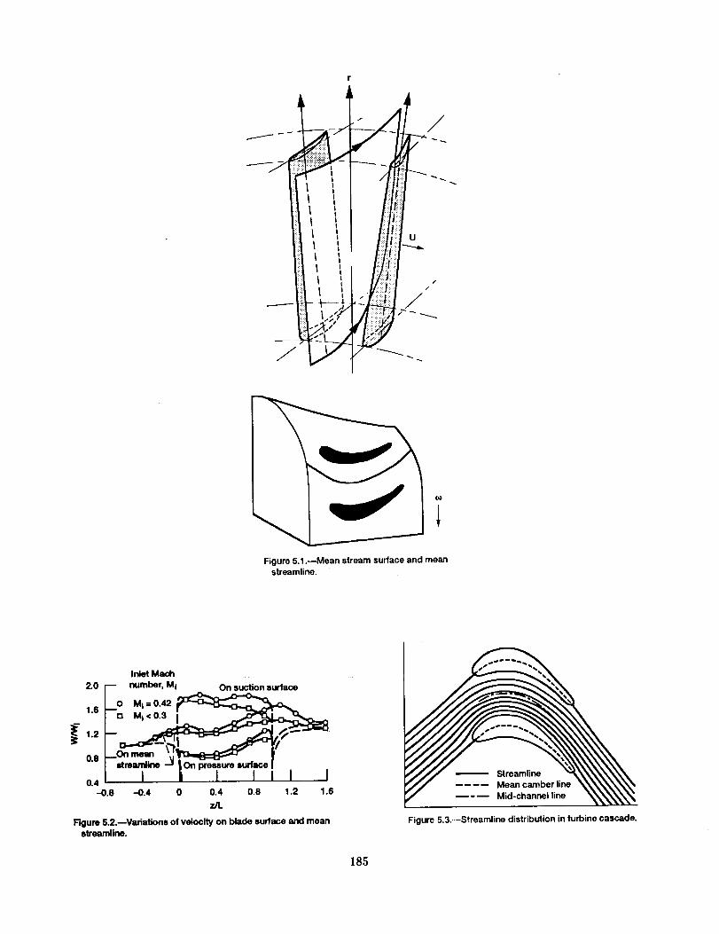
Htiill
Figure 5.1 .--Mean stream surface and meanstreamline.
Inlet Mach
2.0 [-- number, M I On suction surface
16 L 0 Mi=0"42_____
• I streamline --' ton pressure surface / .
o41 J i I I I I I
• -0.8 -0.4 O 0._: 0.8 1.2 1.6
Figure 5.2.--Variations of velocity on blade surface and mean Figure &&--Streamline distribution in turbine cascade.
streamline.
185

1.6
0.8
E(,- 0
_ _ -o.e
-1.6
-.24
T -- Mi=42
± P:t ",_ ----- M_=0__----_ - ----- P/(p-t)
1.4
1.2
1.0
I I I I ] I0.8 -0.4 0 0.4 0.8 1.2 1.6
z/L
Figure 5.4.--Variation of specific mass flow and passage widthratio.
1.6
0.8
N-0.8"_ -1.6
-2.4
-3.2 I
-0.8 -0.4 0 0.4 0.8 1.2 1.6
Z/L
Figure 5.5.--Variation of tangential velocity and Its derivative withrespect to z along mean streamline.
de
dz
s(£)= 0
£6 £8
= constant
£
Figure 5.6.--Mean streamline in the flow passage.
186
1 II

(NACA TN 3448, 1955)
Figure 5.7.---Streamline in a radial-flow impeller.
O Assumption, 50 percent streamline[] First calculation, 65 percent streamline<> Second calculation, 65 percent streamlineA Third calculation, 65 percent streamline1.5 --
1.4
1.3o
_1,2
1.1
1.0 _!_.9 _ I
0 4 8 12 16 20 24
Station
Figure 5.8---Variation of meridional velocity on mean streamline.
1.2
1.0
0.8
,_ 0.6
0.4
0.2
0 0.2
Figure 5.9.--Comparison of velocity distribution around atransonic turbine blade.
• _ {rB)l . .....
Time marching method
O MSLM3termsedes ! ___._.,..
• MSLM 5 term series• Experimental data
I I 0Is 1100.4 0.6 • •Percent _" "-
Figure 5.10.--Family of S2 surface end intersection with inlet
plane ZI.
187

S2m
,/_s,,(+l)
Figure 5.11 .----Family of S2 surface formed progres-
sively from S2.
IZ
16--
x2
15 --
14
13--
12--
11 --
10 --
K0
92
J11
10
9
_1.5
_ 8
7 1
2.5 B
1.5
4
3 _2 0.5
x 17
I I3 4 5 6 7
z, cm
Figure 5.12.--Projection of S 2.m streamlines on mertdional plane(CAS compressor).
// . .o...-.-.---.43.,._
I I I0 0.5 1 1.5 2
z, cm
Figure 5.13,--Blade shape and velocity distrubutlon on J = 3 S 1surface.
I2.5
188
-7 IF

-14
K .12 E.
2 3
10
Figure 5.14.--Intersection of S1 , S 2 surfaces with the throughflow cross sections of turbine rotor.
I-
__ "'J X2
Rgum 5.15.--Transformation of coordinates.
32
28
24
2O
16 I-6 -4 -2 0 2
z, cm
K
10
8
6
4
2
7 J
I I4 6
Figure 5.16.--Projection of S2,m streamlines on meddonalplane (CAS compressor).
189

300 ]-- _ Stress surface extension/
_ expansl_
2oo_150'
E0
-1
-2
-3
-4-3
!
I l I I I-2 -1 0 1 2
Z, cm
Rgure 5.17.--Blade shape and velocity distribution on k-7coordinate surface.
190

.9 [_ _ Present method
/ Complete 3-D solution
.8
.7
J.5
.4
.3 I I I I I I I-3 -2 -1 0 1 2 3
z, cm
Figure 5.18.J--,ompadslon of mach number distribution on k-9S1 surface.
0.4
0.2
&
A _ Present method
014 18 22 26 30 34
Rm, cm
Figure 5.19.--RelaUve twist on J-3 suction surface.
1
X2
Figure 5.20.--Body-fitting quasi-orthogonal C-grid around theblade leading edge.
191
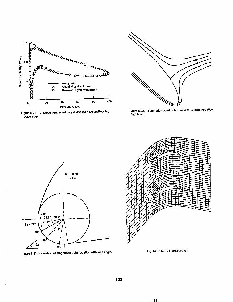
1,5
i 1.0
(_ _ Usual H-grid solution
_ I i ._ I i 10 20 40 60 80 1O0
Percent, chord
Figure 5.21 .---improvement in velocity distribution around leading Figure 5.22.--Stagnation point determined for a large negative
blade edge. incidence.
M 1 = 0.509
¢r =1.5
Pl = 20°
10.5 ° I
29.7 ° 80,4 o
2,o '7!!./_1 350
Figure 5.23.--Variation of stagnation point location with inlet angle. Figure 5.24--H-C grid system.
192
I7IF

-0.2
00
0.2 102O
0.4 3O4O47.3
0.6 5O6O
0.8 7080
1.0 9O
1.2
14 I I i0 0.1 0.2 0.3
Figure 5.25.reDistribution of streamline in a cascade
having splitter vanes.
D or = 1.5(14m.b.) 13.0 ° Calculated value
• 12.2 ° Experiment data----0--- 7m.b. + 7s.b. 11.8 = #s = 47.3
1.0 -"¢"- or = O.75(Tm.b.) 10.7 • -
.9
[ I I.3 I ] I0 20 40 60 80 1O0
Percent, chord
Figure 5.26.--Mach number distribution around blades of threecascades.
Figure 5.27.--S 1 stream filaments. Figure 5.28.uThree-dimensional variation of an S 1
stream filament.
193

Figure 5.29.---$2 stream filaments.Figure 5.30.--S 1 filaments and a mid-channel S 2
employed in quasi-3D solution.
S2,m
I
Convergence Icriterion
IYes
Figure 5.31 .--Calculation steps in quasi-3-D blade design.
194
"I I]

i
I I
B _ I A I
' i
I. I
B _ I A I C
J I4- _ 4i I°
B
I _ A !C
i i°
i i°
Figure 5.32.---Determination of flow condition far upstream and downstream of theembedded blade row.
30
6 25t,:
2O
15
l..__-_ 0 1 2
XI I i
VII1
VII
V1
-- V
f IV
1
5
6 7 8I I
X]
X
IX
VIII
VII
vI
V
IV
I I10 15
z, cm
Figure 5.33.mProjectlon of stator blade and streamlinedistribution on meddlonal plane.
0.10
0.08
0.06
0.04
0.02
_ //'0"
= °
m
m
O Neglecting entropy IncreaseZ_ Considering entropy Increase
I I I I1 2 3 4
Number of iterations
Figure 5.34.mEffect of entropy on consistency.
195

v
9-
°-11f
-0.30 t----0.06
---o-- s, I
S2mi
__ _°00.08 0.10 0.12 0.14 0.16
Z (m)
J0.18
Figure 5.35.--Streamlines on S 1 and $2, m at blade root.
0.2
0
=Z,d
-0.2
-0.4
1
E0 I
/_1_
/
®
@®
®
2 3 4 5 (_)j
S 1 (3) S t (5)
Figure 5.36.--Deviation of general S 1 surface from surface of revolution (magnified ten times).
C
II
E'
"I!
/
196
:1 1 F

11
s
s2--'-
L
s_---"
i_ __.-
A-A
...d
]
2 3 4 5 (AR/R) $1 < 0.5% B-B
Rgure 5.37.--Deviation of generaJ S 1 surface from surface of revolution (schematic).
0.00
0.05
0.10
0.15
0.20
0.25
0.30
Figure 5.38._Streamlines on S1 stream surface (mid-span surface).
Ouasi-3D design
__ Qu_i-3D analysis
I__ i qJ0 40_E_J_ i _ -- _'- Quasi-3D design j---0-.-- FulI-3D analysis I
- _ _. 20 _ I Trailing'°ti",6 8 10 12 14 16 -108 10 12 14 16
z, cm z, cm
Figure 5.39.--Varlatlon of Vet on mean streamline (mid-spansurface).
197

1.12
& 1.08
"_ 1.04
d'._ 1.11tl --II1
0.968
O.-- B/'B k Quasl-3D designB/B k 3D analysisP/(p-t)
Leadir_g edge J
10 12 14 16
Z, cm
Rgure 5.40.--Variation ofB/B k and P/(p-t) on mean streamline(mid-span surface).
1.0 I"- I X_"% Full 3D I
/ Ir -'-,'x ...... Ouas,-3oI
!"r ..... !,.7 " I
.41 I ]1 I I J [ ] ..]1 I-.04 -.03 -.02 -.01 0 .01 .02 .03 .O4
Z(m)
Figure 5.41 .--Mach number distribution over blade surface(mid-apart section).
40
O
s0 -- -- !
I II
II,, I 10
i 8!
_j _ 42
-i I L_I j-10 0 10
20 _--
10 I-20 20
z, cm
Figure 5.42.mMeridional projection of rotor blade, streamlinesand L2F measuring locations.
Percentdesignspcad
1.7 --100
-l
1.o I 1 I J 1 l i I I110 120 130 140 150 160 170 180 190 200
Equivalent mass flow, kg/sec m 2
Figure 5.43.--Compressor overall performance map.
1.6O
1.5
= 1.4
_ 1.3
_ 1.2
1.1
34 --
30 _
E 26 --O
_=_ 22 -
A
0
18--
_) 1 I I141.0 1.1 1.2 1.3
Stagnation pressure ratio
Used in calc. (70% design speed)L2F meas.Conventional measurement
(b) I I __I___I0 10 20 30 40
Outlet angle ¢_2,deg
Figure 5.44.-- Radial variation of stagnation pressure andoutlet angle.
198
--O---
&
£I
E
)
)
14 (a) I I J1.0 40 60 100
Rotor effic!ency, MR
30 m
E 26 --0_
._=
a: 22 --
18--
Used In calc. (70% design speed)Design valueTemp. measure
"7- =
[[[
[[
- 216 24 32
V0r, cm 2/see1
I4O
Rgure 5.45._ Radial variation of rotor efficiency and outlet V or.
_T117

.14
.12Z'
.10
.08
.060 1 2 3 4 5
Number of Iteration
Figure 5.46.--Rate of convergence.
36
32
24
2O
162O
Used In calc. (70% design speed) /_]
_ _ Design value ._//_'
Ji-2
g/
i I 1 JO -20 -40 -60
Ralative angle 13,deg
Figure 5.47.-- Radial variation of _.
I
n_
36 --
32--
28--
24--
20--
16 ____I____i0 0.1 0.2
Outlet Inlet
0.3 0.4 0.5 0.6 0.7 0.8
Ralative Mach number
Figure 5.48.-- Radial variations of relative Mach number.
199

•---0--- Calculation• L2F Measurement
34
_26 ,, 23 24 25
18[ D14 1 ] J I J [ ] 1 I I J
0.2 0.4 0.6 0.2 0.4 0.6 0.2 0.4 0.6 0.2 0.4 0.6 0.4 0.6 0.8 0.4 0.6 0.8
Absolute Mach number
Figure 5.49.-- Radial variation of absolute Mach number at Stations 23 - 28.
60 [-- _ Calculation
! • L2F Measurement
30 Pressure surface
_2o I I
40 -0.2
I -0:+
40 _ 0.130-- 0.2
I Leading Trailing I2o edge I ! I edgel I 0-31_ _ I I i I I I I I0 2 4 6 8 -1 0 1 2 3 4 5 6 7 8
Axial distance z, cm z, cm
Figure 5.50.--Axial variation of relative flow angle. Figure 5.51 .--Lines of constant relative Mach number on No. 3S1 surface.
2OO

\Characteristics
\Passageshock
jS
Starting line
Detached Sonic lineshock
Figure 6.1--Bow wave/passage shock and characteristic net in
a compressor cascade with supersonic inlet velocity,
Physical plane_
;1
,d
a l
a
t
t JI f
g
d
d'
e
Je'
Calculation plane
c 1d
2_d'
4_
6--!II_Le
,_ b.,&_ ,a - .J. - e I
Figure 6.2--Coordinate system used downstroam
of passage shock.
201

\
875
\
Figure 6.3---Streamline distribution and Mach contours.
0.6
04T"_t-_ I I I n
_on"
1.1
d
1.0
0.9
0.8
Mj = 1.11
I I i 1 I I I [ I
L.
E
e--
t-Oeu
1.6
0.8 --
0.4 I I I | I I I 1 1-0.4 0 .04 .08 1.2
Z*
Figure 6.4.--Variations of V0r, I_ and M along three streamlines.
202
"IIV

¢MZ<
0 m
Passage shock,No. 3
From R-H relationFrom subsonic solution
-is I I I ]200 250 300 -45 -55 -65
W m/s J3,dog
(e) Velocity W m/s. (b) Flow direction 13.
Figure 6.5._mparison between result calculated by R-H relations and result obtained in downstream subsonic solution.
1.4
1.2
0 Experimental data[ 82]Sedes expansion[ 58] j_ 1.0
------ Time marching[ 35] J1.2 -- -.,C]-.- Present met_f-
1.0 -- _ - O _ 0.8
j 0.0. 0.0.2° 1 I l I I 0.4
o 0.2 0.4 0.6 0.8 1.0
Percent, chord
Rgure 6.6.--Mach number distribution for turbine cascade.
LI V Present methodRelaxation
-- O Time marching[ s4] _O" x
-- Expedmental data /_ "t
_ _
I I I I I0 0.2 0.4 0.6 0.8 1.0
Percent, chord
Figure 6.7.--Mach number distribution for T 1 cascade.
203

1.4
11.0_0.6 -:" .......
T1 cascade---- Improved T 1 cascade
0.2 I f I I I0 0.2 0.4 0.6 0.8 1.0
Percent, chord
Figure 6.8.---Modification Mach number distribution for T 1cascade.
°,f0.2
0.1 F00.8
TI profile0 Improved T1 profile
1.0 1.2 1.4 1.6 1.8 2.0X, cm
Figure 6.9.--.Odginai and Improved profile.
1.4
1.213.
I
o 1.0
_'0.8 (I
0
_T0.6- _ Calculation
0--- Expedmental data
0.4 I I I I I0 0.2 0.4 0.6 0.8 1.0
Percent, chord
Figure 6.10.--Pressure distribution around the blade.
2O4
1.5
1.0
0.5
>_
0
-0.5
1.4
i 1.2
i 1.00.8
0.6
65
60
=_ 55
5O
q,0.9
......... 0.5
------ 0.1 .-- ...-'- -- _.:.=-,= :. _..
i ii i
I 1 I, [ I I
45-0.2 0 0.2 0.4 0.6 _ 0.8
z" J
Figure 6.11 .--Flow variation along three streamlines.
"--%%,,
I I I I _ I I1.0
:I lli

1.4
_'_ 1.2
t l.G
0,4
0 0.2 0.4 0.6 0.8
Percent, chord
Rgure 6.12.--Pressure distribution around the blade.
1.5
1.0
0.5
--0.5
qJ
0.9......... 0.5------ 0.1
r, ......... _f'--'---':-'-_' ._'_--_-,=._
I- !
!!
- !!
I [ __1
1.4
1.2 - ___ ,........if= '''''I
1.0 _ t,.
o. "',: -:. \
_-_oss- [_._ ,/./
o _:_::_o;da,a ' :='_::::::: :'750 _ I..-_
I I I I 1 4s I I t. I I J1.0 -0.2 0 0.2 0.4 0.6 o.e 1.0
Z t
Figure 6.13._Flow variation along three streamlines.
A 1.0
I
O
0.8!
O
0.6
t "--O-- Calculation, 1"1= 1.04
_" _ Calculation, _[1= 1.1 80 Experience data, suction surface
1.2 D Experience data, pressure surface
D [] 0
0.4 1 I __L_L . I0 0.2 0.4 0.6 0.8 1,0
Percent, chord
Figure 6.14.--Pressure distribution around blade.
205

1.4
1.0
0.6
>_0.2
-0.2
0.9& ...... 0.5
m m _ 0.1 ,.. ....
i j-- I iI iI i
-. I i,_._._.... :.
I I I I I I
s"_ 1.0
0.8
1.4 I _ ,j,fl f'_i
I,,_,'
0.6 f t t I l I
7O
65
6O
55 ¸
50 !
45-0,2 0 0.2 0.4 0.6 0.8
z•
Rgure 6.15.--Flow variation along three streamlines.
n
- _........._=_-'_................_,_ ...... i_.."-_
I I I I I I1.0
S°S.
P.S. P.S. S.S.r T
TqJ
Figure 6.16.--Variation of r and q_ fora general S t surface.
206
::I 1]

r r
Figure 6.17.---General S 1 stream surface.
A.
A3
x 2
Ill
Figure 6.18.--Division of computation region.
D1
xI
(a) Characteristic (b) Computational grid in subsonic
network, flow region,
Figure 6.19.--Merldional projection of characteristic network on
S 2 and mesh on meddional plane for subsonic flow region.
Figure 6.20.--Merldonal projection of streamlines.
207
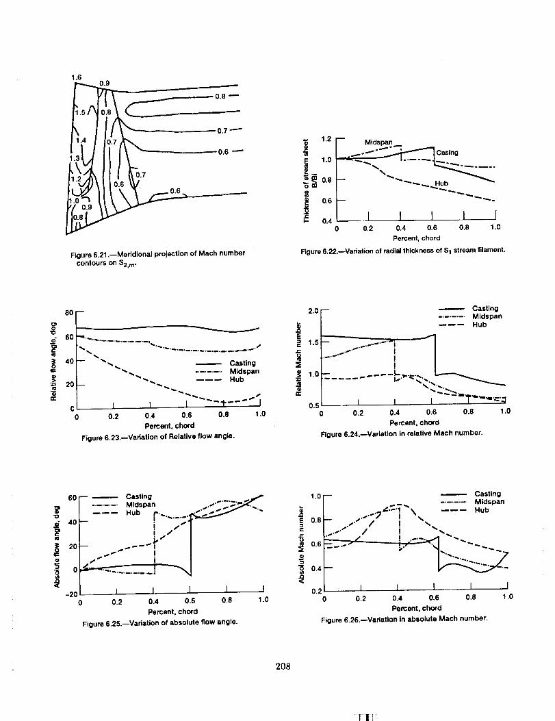
1.6
_0.9 .
3 0.6 --" ---'° , Casing1.0 -..._ I.w-_J
0.6 _"'_._,.,
0.4 I
0 0.2 0.4 0.6 0.8 1.0
Percent, chord
Figure 6.21 .--Meridlonal projection of Mach number Figure 6.22.--Variation of radial thickness of S1 stream filament.contours on $2, m,
8O
60
3 40o
._>20
C0
2,0_
..... _ 1.5
_,_, _ Casting" _ _ - ........ Mid span
_,_,,. _m_ Hub >¢ 1.0
1 I 1 ""1"-"- I0.2 0.4 0.6 0.8 1.0
Percent, chord
Figure 6.23.--Variation of Relative flow angle.
Casting........ Midspan
_ _ Hub
0.50 0.2 0.4 0.6 0.8
Percent, chord
Rgure 6.24._Vadatlon In relative Mach number.
i
1.0
"0
i
dl
I0
5
60
40
20
0
-20 --0 0.2 0,4 0.6 0.8
Percent, chord
Figure 6.25.--Veriation of absolute flow angle.
_ Casting ,, ,,,........ Mldspan ,,," ""_"'L
_ r.- .....i /.-_ =E!// _ =
I 1 I t I1.0
1,0
0.8
0.6
0.4
0.20 0.2 0.4 0.6 0.8
Percent, chord
Figure 6.26.--Variation in absolute Mach number.
Casting
-- _ ........ Midspan•..''=_" "! \ ------ HUb
__ _,, " / I _.
• t===, . _._
, [ 1 I I I1.0
208
'1|1

1,2 --
1.0--
0.8--
0.6
0.4--
0.2--
0
-0.20
Casting........ Midspan
Hub
/
i _.
/ I
i ""_ i0.2 0.4 0.6
Percent, chord
Figure 6.27.--Variation of V0r.
2.0
1.6
O.
o 1.2
0.8==
t_
0.4
I I o0.8 1.0 0
.,i._,w°
row--
CastingMidspanHub
_,l°J
i /
I I I0.2 0.4 0.6
Percent, chord
f'j'
I J0.8 1.0
Figure 6.28.--Variation of pressure ratio.
I
ii.
IIl11_
I IIIIi_ _ _. ,_I
1111__ _ _''I I I__ra,,ooedge
I J Leading edge
(a) Grid used in calculations I and ]i, 61 xl 1.
Shock
=-_ _ge Trailing edge
(b) Grid used In calculation 111,49x11.
Figure 6.29.--Grid system and project of blade and shock onmeridional plane.
209

1.2
0.8-0.5
........ Calculation I! Span,Calculation Ill percent
t-- 20
I I I I0 0.5 1.0 1.5
Axial chord
Figure 6.30.--Input value of T on $2, m"
1.0
0.5
0
_j -0.5
r_ 1.0
0.5
0
-0.5
SCalculation ]l
- #'/ / span,*_' A (_ percent
/'t 4..T'--_-- 7_o/J.../._ _._ - _- 5o
t I I I
SCalculation llI
- f/F / span,Y L_-. pe=e.,
/_-_"--/_.J_i_... "_-- 70
I l I I
........ Calculation II1 IO
------ Calculation l!! (Initial) _ '_
Calculation Ill (flnal)_//
_. Span,0.5 _ _"/_ percent
?- i"_1_ <'- _oi/ ,," /-'-_. "--50
_J,_V, k°0 _-0.5 0 0.5 1.0
Axial chord
Figure 6.31 .--Input value of Ver and s on $2, m"
11.5
210

1.2 1.0 1. 1.0
,'Q_/_'"..,"'--</////A2"'" " ' :','." " "'-_F/////A_"' "''" "'
..(a) Measured. (b) Calculation I. (c) Calculation II. (d) Calculation III.
Figure 6.32.--.Comparison of Mach number contours on $2, m.
1.0
.853
.714
.597
.46G
,355
.Z72
.123
• 05g
0
Calculation I
- _ Calculation il
Calculation Ill
Figure 6.33.--Comparison of streamline distributions.
Calculation |I
Calculation |II
0.10 [_ LE.
!-:::_o.._,-;-'+'"'w"-"f_"_
0.12 f L.E =_=
0.10
t-" 0.08
0.08 ='355 I I I
o.1,I _ ,.EoE 0.12 _,..,.,..__''" T.E.
t: 0.10 = 1230.08 ' I I 14 6 8 10 12
Z, cm
Rgure 6.34.--Variation of filament thickness (1 percent mass
flow).
211
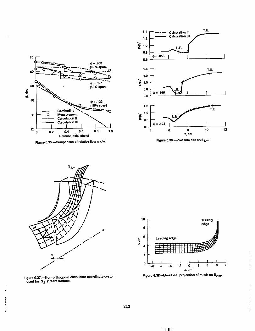
¢0.
7O
qJ= .ss3..... ._ (89%span)
60 _. ""
50 _\ _ = _597
_'_,.__:_ " 168% span)
.... Carnbedine _'..30 _ 0 Measurement _._
-_ Calculation I] _..Calculation I|!
20 I I I I \',, i0 0.2 0.4 0.6 0.8 1.0
Percent, axial chord
Rgure 6.35.---Comparison of relative flow angle.
1.4
1.2
•_. 1.0
0.8
0.6
1.4
1.2
, 1.0
0.8
0.6
1.2
_ 1.00.8
O.6
T,E.__-_ Calculation II
-- Calculation Illf '
(
='_31 I I
I T.E.='123 I I ]
4 6 8 10
z, cm
Figure 6.36,--Pressure dse on $2, m.
I12
f
¢o .J
j"B
f
Figure 6.37.--Non-orthogonal curvillnear coordinate systemused for S 2 stream surface.
EU
10
8
6
4
Trailing m
edge J
Leading edge
II ::
2
0 ] I I ] I I I .I•-8 -.6 .-4 -2 0 2 4 6
z, cm
Figure 6.38--Meridonal projection of mesh on $2, m.
212
I lr

0 _dn_t_ data1.4 r- _ AS and flow rite 1.0
J oorreot_n1.2 _ _- _ AS oormidemd 0.8
I I-I:) --- k_i_,:_o.u.o,, iF -_.o. o_'_ "',--.. _ 0.4
0.6 .2
,_,!__L___L _0 0.2 0.4 0.6 0.8 1.0 0 0.2 0.4 0.6 0.8 1.0
F_um 6._.--_ff_ of entropy lind flow m_ correction. Figure 6.40.--4r_'_ in Ver .a_ casing.
Trailing8 edge
4
Leading edge
I.IS !.2 1.251.3
1.00.9
0.8
0.8
0.7
0.6
).5
0 I I I I I I I I I
-3 -2 -1 0 1 2 3 4 5 6Z, cm
Figure 6.41--Meridonal projection of MaC h number contours.
213

Accurate solution
Relaxation factor a = 1
Relaxation factor ,_ << 1
_..__.... (n ÷ I)., _
"_..:_--
_e
v
z
Figure 7.1 ._Local fluctuation of S 1 stream filament thick-
ness during iteration and the effect of relaxation factor
(sketch).
/--- 2nd cycle
/ /-- 4th cycle f-- 8th cycle//
r ,,hcycle/
3rd cycle --/
z
Figure 7.2.--Variation of tip S 1 filament thickness (schematic}.
St.
2O
15
10
(a}5
0
I I I I Co) t I
5 10 15 20 0 5 10
Z. cffl
(a) 1st cycle.
Co)_h cycle,7iguce 7.3.--MeridionaJ projection of streandines obtmed on S2. m surface.
I I15 20
214
_I 11

2.0
i 1.5
1.0
t-" .5
Blade height,percent
,._ 0
_ _,,,....\"/_'I_ -- 70
_ --_-_ _ "%_
(a) I I10
Co)I I
15 20 0
Z_ cm
(a) 1st cycle.(b) 9th cycle.
Figure 7.4.--S 1 filament thickness.
Blade height,percent
...._ 0
---- 10
. _ 30
_-- 50
.---- 709O
I I I I5 10 15 20
P-,
£
1.4
1.0
0.6
0.2
-0.2--5
1_ Percent
bladeheight
I I I I
15 20 -55 10
z, cm
(a) 1st cycle.
blade
height
II I0 5 10 15 20
Zj cm
(b) 9th cycle.
Figure 7.5.--S 2 input Vor.
1.1
1.0
co";_ 0.9-
0.8--
0.70
Blade
height,percent
_ "_ 100
I I10 15
z, cm
(a) I st cycle.
I2O
Bladeheight,
/_ percent"_" _ O
_-_-.. _- ,507o
_f "-- 90..... IO0
0
I I5 10
z, cm
(b) 9th cycle.
I I15 20
Figure 7.6.--S 2 Input filament thickness.
215

1.8
1.4
11.0
i0.6
Bladeheight,
-- percent
/-- 0
r- 10.///-- 3o
IIL , , Jr,oo
0.2 I0 5
Bkkdehe_ht,percent
/-- 0/r- 10
- .i_'_ ///-- 3o_-"---'--"-'J"-UI i Ii._ so
I #"_111 -/II_ 70
I I I I_ J10 15 20 0 5 10
z, cm z, cm
(a) S1 calculation. (b} S2 calculation.
Figure 7.7.---Output Mach number on streamlines of 9th cycle.
I I15 20
(1) (3) (2)
(a) 18 percent blade height.
(1) (2) (3)
(c) 68 percent blade height.
°l
(1) (3) (,2)
(b) 45 percent blade height.
(1) (2) (3)
(d) 89 percent blade height.
Figure 7.8.--Mach number contours on S1 surface: (1) DFVLR measured data; (2) calculated by pref,ent method; (3) from Ref. 34.
216
"I-1!7

I I I An_
0 nMmaCb_hr 1 0
0 --_,,_; ? Calc ul.._rad:_a _ ?etGe0''-
0 (a) Mach number. 0 (a) Row number.
Figure 7.9.--Radial vadatlon of Mach number and flow angle at a number of stations.
Pressure surface Centrel-mld-surface Suction surface
Rgure 7.10.--Constant Mach number contours o.n three S 2 surfaces.
217

3O
70 _ Percent span
Figure 7.11--Variation of flow angle along three stream lines on
$2, m surface.
.9
'2 :_.o
0.9
0.8
- 0 18
0.6
Calculated
20 I I i [ I
0 20 40 60 80 100 10 50 90
Axial chord, percent Percent, chord
Figure 7.12.---Constant Mach number contours on span-wisesurfaces formed by (x 2 x3) coordinates.
Figure 7.13.--Three-dimensional passage shock.
218
_l |17
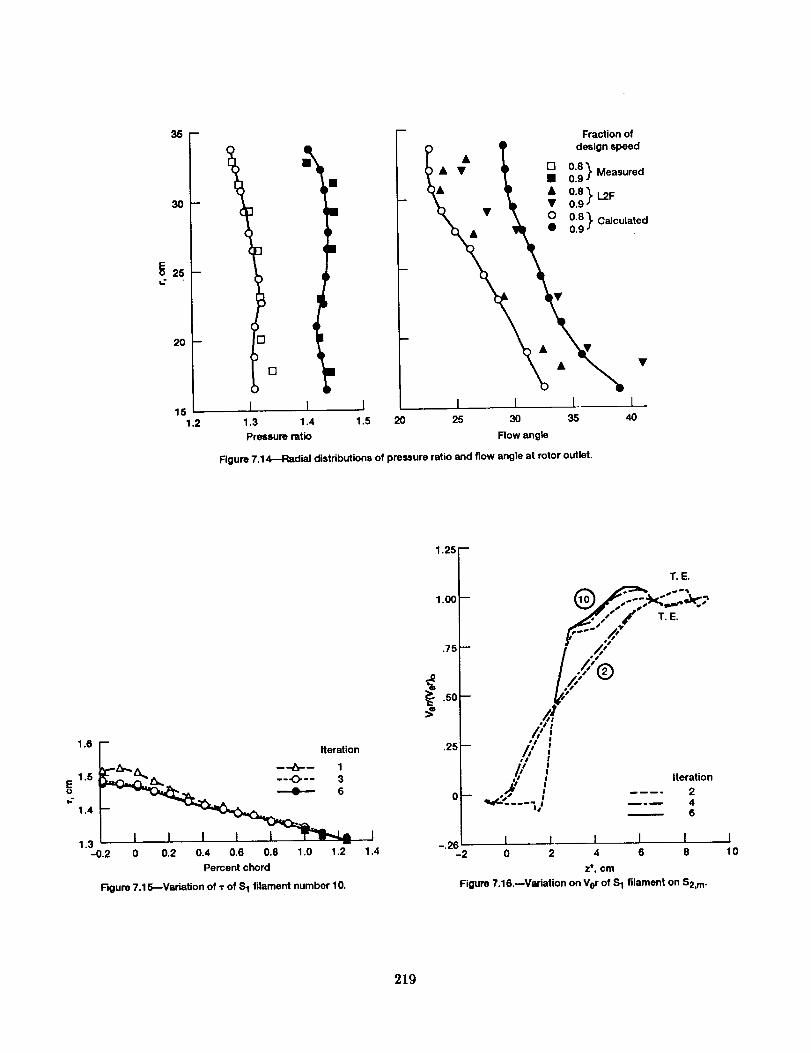
35
30
25=Z
20 --
151.2
II
)
D •
)
I1.3 1.4
Pressure ratio
I1.5 20
-- Fraction of
? T design speed• T& [] 08
t • 0"9)Measured
- • 0.9.'\ ? °-8}c=,cu,atod
I I [ I25 30 35 40
Flow angle
Rgure 7.14.--Radial distributions of pressure ratio and flow angle at rotor outlet.
1.6 F Iteration
_I_I_Z_,__ ---'_--- 1
oE 1.5 ._.z(_b==CL--_._, . --'0"- 3
1.4
11.3
-0.2 0 0.2 0.4 0.6 0.8 1.0 1.2 1.4Percent chord
Figure 7.15---VariaUon of T of S1 filament number 10.
1.25
1.00
.75 --
.50 --
.25 --
0 u
-.26-2
T,E°
T.E.
q_c_'-_/!it i Iteration---- 2
.._ m.m 46
I I I I I0 2 4 6 8
z*, cm
Figure 7.16.--Variation on V0r of S1 filament on $2, m.
110
219

$1 S 1
1.4 $2 $2J-- Leading edge
_ _._1.2.0 Leading edge J--_L__{_1_1)___- _.._..... ..__i----.... "_ "/_• Trailing edge Trailing edge
04 t lj2 112
Z, cm Z, cm
(a) Ouasl-3.O. (b) Full-3-O.
Figure 7.17--Mach number along Intersecting streamlines between S 1 and S 2.
40 --
35 --
30 --
_ 25
15
(a)10 -
-10
m
Jr
_ I
, !
I
I I I I __) I I-5 0 5 10 -10 -5 0
Z, cm
(a) Ouasi-3D.
(b) FulI-3D.
Figure 7.18._Meridional projection of streamlines on S 2.m.
I I5 10
220
-I 11;

1.2
1.1
1.0
i-
0.9
0.8
Ca) I I I I (b)0.7
-4 0 4 8 12 -4 0 4z, cm
I I I I8 12
(a) Quasi-3-D.(b) Full 3-D.
Rgure 7.19.--Variation of S 2 filament thlckness along mean streamlines on six S 1 surfaces.
1.2
0.8
_0.4
0
{a)-0.4
-4
(11)
I I I0 4 8
l (b)12 -4
z, cm
(a) Quasl-3-D.(b) Full 3-D.
(11)
I I I0 4 8
Figure 7.20.--Variation of Ver along mean streamlines on six S 1 surfaces.
I12
221

(4)
(1O)
Full 3D
,,,,- ,-,- Quasi-3D
,,,,.e,-, L2F
Figure 7.21 .--Circumferential variations of Mach number.
(a) (b_
( (d) t_, I ._q
/
Figure 7.22.--Iterative process in 3D solution.
222
':F ]1-1

1.4 Leading 1.4 Leading
edge 1 edge 2
.... _ ....._ "_! Trailing
1.0 __ /'_L edge....... _. r,, edge _= 1.o J'_ Tr_,.g
=+o.,.... -__/_ +o.,_0.4 1 1 I 0.4 12 I I _'--"-- _ "" "" _- _ I
-12 -8 -4 0 4 8 12 - -8 -4 0 4 8 12
z, cm z, cm
1.4 I- Leading 1.4 Leading/ edge 3 edge 4
1.2 _- ---"_"_--_--_...,,_t_ 1.2 .....
1.OJ- _/_/_ edge _J \\\_S edgeo.,I__---__ ---+ _.__.__:°.°[_
0.4 / I I I t I ] 1 12/ I I I | I J
-12 -8 -4 0 4 8 12 -8 -4 0 4 8 12
z, cm z, cm
1.4 I- Leading Leading
/ _ 5 edge _/_ 1,= 6
Trailing -- _ _ _ _ ^ Trailing
, o.,r___-_ __-__ ,_...-,_._,_0.6_ _._._j_.__--.=,,,_0.4 l I 1 I I ! , I [ I I I J
-12 -8 -4 0 4 8 12 -12 -8 -4 0 4 8 12
1.4
1.2
E 1.0
e.
•5 o.8I
0.6
0.4-12
z, cm
Leading
edge
z, cm
7-- S t
Trailing --- $2
edge
0 4 8 12
Z, cm
Figure 7.23.--Mach number on S 1 and S 2 surfaces.
223

Percentchord
Full 3DQuasi-3D
Figure 7.24.--Ten S1 stream filaments.
Full 3DQuasi-3D
Percentchord 0 0.5 1.0
Figure 7.25.--Intersection of S 1 stream surfaces with threespan-wise surfaces.
224
'l l!

Figure 7.26.mMach number contours in six S 1 stream filaments.
0.9 1,25 1.0
1.__' _._
'O fg1.00.9
0.9 0.6
o.,_--_W//o..;_ \ o., I_O. 0"6__ "`'``'_
0.6_
111 (Iv) (vii)
Figure 7.27.---Mach number contours in three S 2 stream filaments.
225

Rgure 7.28.--Three-dimensional shock.
PS
i0.5
(5) (g) (11 )
Figure 7.29.--Mach number contours on five span-wise surfaces.
226
(2_)
=
_Ill

(0) (2) (6) (10)
Rgure 7.30.--Constant cr contours on five span-wise surfaces.
1,2 --
(11 ) Leading Trailing
edge edge
1,_1o_/_)_ ____1...... s,(,_w._l_ i....'_
0,= :io.s I I
1.3
1.2
1.1
1.0
0.9
0.8
(7)
Leading
edge
Trailing
edge
I
I I
1.3
(1)
1.2
1,1 --
1.0 --
0.9 --
0.8 --
0.7-0.05
Illl, ,.!i I I jI I • / '_
_._ f / Trailing
Leadi__ / edge
edge___JI _1 I
0 0.05 0.10
z*
Figure 7.31 .--Chordwise variations of S 2 filament thickness.
227
(21)

1.4
1.2
1.0
0.5
-0.5
mLeaSing Trmlingedge edge
Jl//---'--._o:.-_
1,0 _
0.5--
0 -
-0.5
(7)Leasingedge
I
]
I
f / edge
! !/i
I
1.5 w
(1) I
L°asing ./._-'"" iedge J" I
I .."J_', TriCing
._/ edge
1.0
0.5_
0 --
I
-0.5 ! I I-0.05 0 0.05 0.10
Z"
Figure 7.32.--Chordwlse variations of Vet onS2 surfaces.
228
_1 1 i;

Figure 7.33.--Comparlson of Mach number contours on S2m.
229

Form Approved
REPORT DOCUMENTATION PAGE OMBNo.0T04-0188
PuI_C rel_rting I_rdvn for th_ oo41ection Of in/otma|ion is est_',ated to ave*"age 1 hour per rospot_e, including the tim_ for re'_hvlng w_structions, se,_'ching existing data soutclls,
gather_ Ind _n_l the data needlKI, and completing ..a_l reviewing the .c_lecfion of i_ormatton Sm1¢1 c_o_.n,merits m_ing _is but den eslirnate (x any _ aspe¢l Of thiscollection Of inlom_ion, m,cluding suggestm*'_s for reduong this buKlen, to Wul_r.gton Headquarters Se_ces. Directorate k_r ,r#orr_tion Ol:,etaUorm and Re_'ts. f215 JeffMson
ORv_ Highway, Suite 1204, Arlington. VA 222024302. and to the Office o_ Man_menl and Budget. Pa_:)41nk_ P.educ_ion Protect {0704-01M). Washington. OC 20503.
1. AGENCY USE ONLY (Leave b/at)k) 2. REPORT DATE 3. REPORT TYPE AND DATES COVERED
Hay 1993 Final Contractor Report
4. TITLE AND SUBTITLE S. FUNDING NUMBERS
A General Theory of Two- and Three-Dimensional Rotational Flow in
Subsonic and Transonic Turbomachines
lL AUTHOR(S)
Chung-Hua Wu
7. PERFORMING ORGANIZATION NAME(S) AND ADDRESS_I[S)"
Clemson University
Department of Mechanical Engineering
Clemson, South Carolina 29631
9. SPONSORII_C_/MONITORING AGENCY NAilES(S) AND ADDRESS(ES)
National Aeronautics and Space Administration
Lewis Research Center
Cleveland, Ohio 44135-3191
WU 505"90-21
WU 335-05-01
G NAG3-1072
L PE RFOR MIN_I' 6 I_GANIZATION
REPORTNUMBER
E-7267
llL SPONSORING/MONffORINGAGENCY REPORT NUMBER
NASA CR-4496
Sl. SUPPLEMENTARYNOTES
Project Manager, Lonnie Reid, Internal Fluid Mechanics Division,(216)433-3606.
Ilia. DIs_ ,,_,_-_u=uT ' --_ DISTRIBUTION CODE
Ualc h_r general release
Subject Category 02
13. ABSTRACT (Maximum _)0 words)
This report represents a general theory applicable to axial, radial, and mixed flow turbomachines operating at subsonic
and supersonic speeds with a finite number of blades of finite thickness. References reflect the evolution of computa-
tional methods used, from the inception of the theory in the 50's to the high-speed computer era of the 90's, Two kinds
of relative stream surfaces, S i and S z, are introduced for the purpose of obtaining a three-dimensional flow solution
through the combination of two-dimensional flow solutions. Nonorthogonal curvilinear coordinates are used for the
governing equations. Methods of computing transonic flow along S_ and S z stream surfaces are given for special cases
as well as for fully three-dlmensional transonic flows. Procedures pertaining to the direct solutions and inverse solutions
are presented. Information on shock wave locations and shapes needed for computations are discussed. Experimental
data from a Deutsche Forschungs- und Versuchsanstalt fur Luft- und Raumfahrt e.V. (DFVLR) rotor and from a Chinese
Academy of Sciences (CAS) transonic compressor rotor are compared with the computed flow properties.
14. SUBJECT TERMS
Turbomachinery; Design; Analysis; Quasi-3D; Transonic; Subsonic
17. SECURITY CLASSIFICATIONOF REPORT
Unclassified
IlL SECURITY CLASSIFICATIONOF THIS PAGE
Unclassified
IS. SECURITY CLASSIFiCATiONOF ABSTRACT
Unclassified
NSN 7540-01,-280-5500
18. NUMBER OF PAGES
24416. PRICE CODE
IlL LiiiTATION i_ ABSTRACT
Standard Form 298 (Rev. 2-89)Prescribed by ANR,I Std. Z39-18298-102