558

A GENERAL THEORY OF THE AUTOGYRO.

By H. GLAUERT, M.A.

Presented by the Director of Scientific Research Air Ministry.

Reports and Memoranda No. 1111.

(Ae. 285.)November, 1926.

Summal'y.-(a) Introductory.-An autogyro obtains remarkably high liftforces from a system of freely rotating blades and it is important to developa theory which will explain the behaviour of an autogyro and will provide amethod of estimating the effect of changes in the fundamental parameters ofthe system.

(b) Range of Investigation.-A theory is developed depending on theassumptions that the angles of incidence of the blade elements are small, thatthe interference flow is similar to that caused by an ordinary aerafod, andthat only first order harmonics of periodic terms need be retained in theequations. An alternative method of analysis by considering the energylosses of an autogyro is developed in an appendix to the main report.

(c) Conclusions.-The maximum lift coefficient of an autogyro, using thedisc area as fundamental area and the forward speed as fundamental speed,lies between 0 .5 and 0·6 in general, and the best lift-drag ratio is of the orderof 6 or 8 at most. Also, owing to the necessity of maintaining a sufficientratio of tip speed to forward speed, the stalling speed of an autogyro mustrise with the maximum speed of level flight, and so the principal merit of theautogyro system, the low landing speed, would disappear in the case of highspeed aircraft.

(d) Further developments.-The analysis is confin"d to the case of bladesof constant chord and angle of pitch, but there would be no difficulty inextending the theory to tapered and twisted blades, provided these variationscan be expressed in a simple mathematical fonn. It is not anticipated thatan improvement of more than a few per cent. could be achieved by any suchmodifications.

•

Contents.

1. Introduction2. Motion of the blades3. Interference flow4. Flow at blade element5. Thrll~t ..6. Thrust moment and flapping7. Torque ..8. Longitudinal force9. Lateral force

10. Periodic induced velocityI I. Lift and drag ..12. The ideal autogyro13. Maximum lift coefficient14. Maximum lift-drag ratio15. General discussion

PAGE.

559560562563565567568569571571574575577578579

I. Introduction.-The lifting system of an autogyro or gyroplaneconsists essentially of a windmill of large radius R with three ormore identical bl~des. whose angular rotation Sl, is maintained bythe forward speed V of the aircraft. Each blade is also free to rotateabout a hinge at its root which is normal to the shaft of the autogyro.In the simplest case, the chord c of the blades is constant from rootto tip, and the blade is attached to the shaft at a small positiveangle of pitch tl, while the shape of the blade is concave downwardswhen viewed from front or rear. The shape of the blades will beassumed to be of this simple form in the subsequent analysis,although in practice the corners of the blades are rounded off at thetips and the chord tapers to the dimensions of the spar at the root.Variations of the chord and angle of pitch along the blade would notnecessitate any fundamental changes in the method of analysis, butwould involve greater complexity at all stages.

When the shaft of the autogyro is inclined backwards at angle i(fig. 1) to the normal to the direction of motion, the autogyro willbe said to be at angle of incidence i. The resultant force actingon the autogyro can then be resolved conveniently into the fonowingcomponents ;-

T, the thrust along the shaft.H, the longitudinal force at right angles to the shaft III the

plane of the shaft and of the direction of motion.Y, the lateral force, normal to the previous components and

positive to the side on which the blades are advancing in thedirection of motion.

The lift Z and the drag X of the autogyro are expressed simplyin terms of the thtust and longitudinal force by the equations ;-

Z = T cos i - H sin i } (1)X=Tsini+Hcosi

559

Appendices.

\. The energy losses of an autogyro2. Conditions for maximum speed3. Vertical descent4. Notation

Tables.

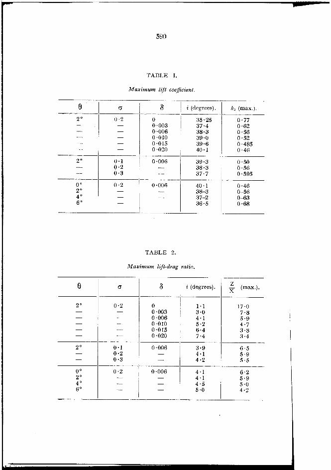
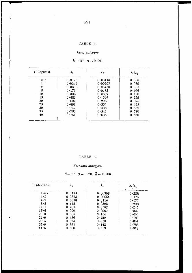
I. Maximum lift coefficient2. Maximum lift-drag ratio3. Ideal autogyro4. Standard autogyro ..

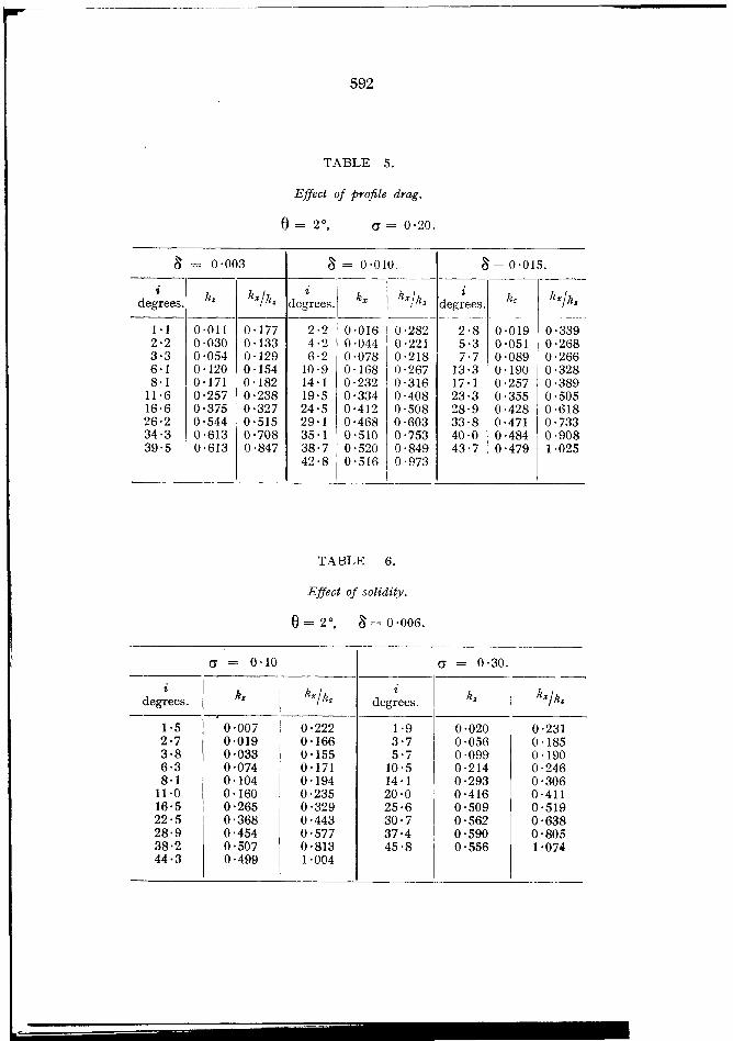
5-7. Effect of profile drag, solidity and angle of pitCh ..

PAGE.581586588589

590590591591592

560

The relationShips between the two sets of coefficients involves asingle parameter A, which is the ratio of the forward speed to thetip speed

(5)

(4)

(2)

(3)

vOR

A=

and in particular the equations (I) become

A 2k, = T, cos i - H, sin i lA2k. = T, sin i + H, cos i f

It may be noted that the angle of incidence i and the speedratio Adefine the state of working of the windmill.

On the other hand, when considering the motion of the aircraft asa whole, it is necessary to use the forward speed V as fundamentalspeed, and to define the non-dimensional coefficients of drag, lateralforce, and lift by the equations

X = k. 7t R2 PV2 }Y=ky 7tR2 p V2Z = k, 7t R2 P V2

2. Motion of the blades.-Each blade is hinged at its root aboutan axis normal to the shaft of the autogyro. The plan form of theblades is approximately rectangular, but the blades are curved soas to be concave downwards. Take the line joining the root to thetip as base line (fig. 2), let h be the ordinate at radial distance r, andlet X be the slope of the tangent at this point, so that

dhX= d r

Owing to the method of attachment of the blades to the shaft,the only couple which can be transmitted to the autogyro is atorque Q about the shaft. The torque will be regarded as positivewhen it opposes the rotation of the autogyro.

In order to express these force components in the form of non­dimensional coefficients, it is convenient, when considering theaerodynamics of the rotating system, to use the disc area 7t R2 ofthe windmill as the fundamental area and the tip speed {J R as thefundamental speed. Accordingly, non-dimensional coefficients aredefined by the equations

T = To 7t R2 pO 2R2 }H = H,7t R2 P02R2Y = Y,7tR2 p02R2Q = Q, 7t R 2 P0 2R 3

561

(7)

(6)

(8)}

~ = 0·0024

~ _ ~o2~ - :{--

1)1 = 0'02,

JR. Xdr = 0

JR. JRXr dr = - • h dr = - 1)1 R2

JO

R JRXr 2 dr = - 2 0 h r dr = - 21)2 R 3

JR. X2 r dr = ~ R2

G1 = ( m g r dr = fl.l WI R

rR W

11 = m r 2 dr = fl.2 -' R2.• g

J, = rR

m h r dr = € 11..

and for the purposes of the analysis the curvature of the blades iscompletely represented by the values of the three coefficients,1),. 1)2' and ~.

The flapping of the blades also depends on the following threeintegrals, involving the line density m of the blade and the totalweight W, of one blade:-

In the subsequent analysis the values of the following integralsare required, depending on the curvature of the blades :-

The general analysis will be deVeloped in terms of the sixcoefficients defined by equations (6) and (7), but in numericalapplications it will be assnmed that the blade has the shape of acircular arc and that the line density m is constant along the blade.In this special case € is the camber of the circular arc and the othercoefficients have the values

A typical numerical value for €is 0·03 and then

The position of a blade at any moment can be defined by theangle tjJ through which it has rotated about the shaft from thedownwind position and by the angle ~ which is its upward inclinationabove the plane normal to the shaft. Then, provided that the

I )

562

angles ~ and Xare small, the equation of motion for the flapping ofthe blade is

[mr2~ dr = [dElrdr - [mgr dr-rm02r(r~+ h) dr

or

II (~ + 0 2 ~) = (™h - GI - 02Jlwhere the suffix (1) denotes that the values refer to a single bladeand where (TM), is the moment of the thrust about the hinge of theblade.

The angle ~ can be expressed quite generally in the form of theFourier series .

(10)(TM) 1 Q2 RRW = IJ-l + 1J-2 (~o + c:) -, g

~ = ~o - ~1 cos (<)I - <)11) - ~2 COS 2 (<)I - <)12)where ~" ~2 etc. may be assumed to be positive. For the presentit is proposed to retain only the firsf harmonic term, so that theflapping is equivalent to a tilt of the plane of rotation through anangle ~, with the lowest point in the angular position <)I" combinedwith a general upward tilt of all the blades through the coningangle ~o' On this basis

~ = ~o - ~l cos (<)I - <)11) (9)

and, by virtue of equations (7), the equation of motion for theflapping of the blades reduces to

Hence, to this order of approximation, the moment of the thruston a blade about its hinge is independent of the angular position <)I,and the evaluation of the angles <)I" ~o, and ~, follows from theconsideration of the aerodynamic expression for the thrust moment.

The subsequent analysis is based entirely on the assumptionthat it is sufficiently accurate to retain only the principal oscillationof the flapping, and to neglect all higher harmonics involving cos 2 <)I,cos 3 <jJ, etc.

3. Interference flow.-An autogyro at angle of incidence i isessentially a windmill descending with the axial velocity V sin i andwith the velocity of sideslip V cos i, but owing to the fact that thevelocity of sideslip is considerably greater than the axial velocity,the induced velocity due to the system of trailing vortices willcorrespond more closely to the induced velocity of an aerofoil thanto that usually associated with an airscrew and its slipstream. Theprincipal force component is the thrust T and so the induced velocityv will be assumed to be parallel to the shaft of the autogyro (fig. 3).

563

(11)v = 27tR2 pV'

In the first place also, this induced velocity will be assumed to havea constant value over the whole disc of the autogyro, and the con­sideration of the effect of variation of the induced velocity will bepostponed to a later stage (Para. 10).

The resultant velocity V' experienced by the autogyro is theresultant of the forward speed V and the axial induced velocity v,and may be written in the alternative forms

V'2 = (V - v sin i)2 + v2cos2 i= (V sin i - V)2 + V2 cos2 i

The formula proposed for the axial induced velocity is

T

which is a logical generalisation of the ordinary aerofoil formula.When i and T are small the formula gives approximately

Tv = ---=

2 7t R2 P V

which is the standard formula for the normal induced velocity of anaerofoil of semi-span R giving the lift T, and when i is nearly 90° itgIves

T = 2 7t R2 P (V - v) 11

which is the ordinary momentum formula for an airscrew. It isanticipated therefore that the formula (11) will be valid over a widerange of angle of incidence.

The axial velocity through the disc of the autogyro is

u=Vsini-v

and it is convenient to write

Vsini-v=u=QRx (12)

The equation (II) for the induced velocity may then be expressedin the form

Asini=x+vA2 cos2 i + x 2

(13)

and for small angles of incidence a good approximation can beobtained by neglecting x in comparison with ACos i.

4. Flow at blade element.-Consider the element dr at radialdistance r on the blade which is at angular position VI to the down­wind position. Due to the flapping of the blade and to its curvaturethe blade element is inclined at the small angle (~ + iJ to the

564

normal to the shaft. Now the velocity of the air relative to theautogyro has the components" along the shaft and V cos i normalto the shaft. while the blade element is moving whith the angularvelocities n about the shaft of the autogyro and ~ about the hingeof the blade. The velocity of the air rehLtive to the blade element hastherefore the following components (see fig. 4) :-

(I) normal to the shaft and to the element dr

U cos <I> = Q r + V cos i sin <jI(2) normal to this first component and to the element dr

U sin <I> = u - r ~ - (~ + X) V cos i cos <jI(3) radial along the element dr

u (~ + iJ + V cos i cos <jIThe radial velocity component will be ignored. Retaining only

first harmonics of the angle <jI and regarding the angle <j> as small,the other two components become

U=Qr+Vcosisin<jl }<I> U = Q Rx - Q r ~l sin (<jI - <jII) (14)

- (~o + X) V cos ~ cos 'P

and to this same order of approximation

U2 = Q2r 2 + 2.0 r V cos i sin t<I> U2 = Q2Rrx + 2.0 R x V cos ~ sin <jI

- Q2r2 ~l sin (t - <jII) - Q r (15)(~o + X) V cos z cos <jI

<l>2U2= Q2r2x 2 - 2.02 Rrx ~l sin (<jI - <jII)- 2 Q Rx (~o + iJ V cos i cos lji

The assumptions on which these formulae are based clearlybreak down towards the root of all of the blades and over a widerrange of the retreating blades, since the angle <j> ceases to be small,while on the inner portion of the retreating blade the air flow willactually strike the rear of the aerofoil section, The failure of theapproximation towards the root of the blade is not of any practicalimportance, but the method of analysis will cease to be valid whenthe approximations break down over a large part of the retreatingblades. It is not possible to assign an exact limit to the validity ofthe approximations but it is proposed to take the condition that thevelocity component U cos <j> must be positive over tbe outer half ofthe retreating blade. On this basis the limit of validity is that

V cos in R <! (16)

l'I

"

1"Ii

Ii""

1I

565

The lift and drag coefficients of the aerofoil section correspondto two dimensional motion at the angle of incidence

oc=6+q,For small angles of incidence the lift coefficient is simply pro­

portional to the angle of incidence, since the aerofoil sections are ofsymmetrical shape. Also, the drag contributes only a small correctionto the force components due to the lift, and it is therefore legitimateto replace the actual drag coefficients by a mean value I). This valuewill, howevcr, be greater than the profile drag coefficient of theaerofoil section at small angles of incidence, since it must takeaccount of the increased drag coefficients which occur on the re­treating blade where the angle of incidence is large. The analysiswill be developed on the assumption that

kL = 3 (6 + 1» } (17)kD = I)

The assumption that the lift coefficient is simply proportionalto the angle of incidence will cease to be valid if the angle of in­cidence rises to the neighbourhood of the critical angle. Now thesymmetrical aerofoil sections Gottingen 429 and R.A.F. 30 stall atan angle of incidence of 9° or 0 ·16 radian in two dimensional motion,and hence the limit of validity may be taken to be

6+q,<0·15Ignoring periodic terms, equations (14) give 1> = xR{r and if the

blade elements are to operate below the critical angle over theouter halves of the blades, it is necessary that

6+2x <0·15 (18)This condition imposes an upper limit to the angle of pitch 6 for

which the method of analysis is valid, and on inserting the valuesof x determined at a larger stage (Para. 7), the following limits areobtained.

I) = 0·0046 = 7·8

0·0067·4

0·0087·0

0·0106·6 degrees.

5. Thrust.-For one blade of the autogyro

dT_1 = 3 (6 + 1» c P U2

drand by virtue of equations (15)

3 (fl + 1» U2 = 3 n" (6 r2 + X R r), + . <jJt3 (2 6 r + X R) n V cos i ~

Sill _ 3 n2 r 2 ~1 cos h (19)

+ cos <jJ 3 n2

;~: (~~ ~ X) V cos i

I'

566

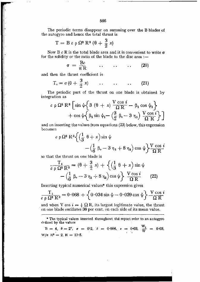
The periodic terms disappear on summing over the B blades ofthe autogyro and hence the total thrust is

T = Be p 0 2 RS (0 + ~ x)2

Now B c R is the total blade area and it is convenient to write afor the solidity or the ratio of the blade to the disc area :-

Bea = 1t R (20)

and then the thrust coefficient is

(21)

(22)

The periodic part of the thrust on one blade is obtained byintegration as

e p 0 2 RS [sin 1Ji{3 (0 + x) V~o~ i - ~1 cos 1Ji1}

+ cos <jJ{~1 sin 1Ji1- (~ ~o - 3 "1)1) VOc~ i}]and on inserting the values from equations (23) below, this expressionbecomes

cp0 2 Rs{(} 0 + x) sin <jJ

- (~ ~o - 3 'Ill + 8 "1)2) cos IJi} Vd~ i

so that the thrust on one blade is

e p ~~ R 3 = (0 + ~ x) + {G 0 + x) sin <jJ

- (~ ~o - 3 "1)1 + 8 "1)2) cos 1Ji} V~~ i

Inserting typical numerical values· this expression gives

T { }VcoSiepO~R3=0'068+ 0'034sin<jJ-0'039coso/ OR

and when V cos i = ~. n R, its largest legitimate value, the thruston one blade oscillates 38 per cent. on each side of its mean value.

* The typical values inserted throughout the report refer to an autogyrodefined by the values

B = 4, 0 = 2°, t1 = 0"2, 6 = 0·006..• = 0'03, ~ = 0·03.

WI" R' = 2, R =17'5.

"

I )

: I: I

I

567

6. Thrust moment and ftapping.-For one blade of the autogyro

r dT 1 = 3 (6 + <1» c P U2 rdr

and according to the analysis of Para. 2 the thrust moment must beindependent of the angle <./J and have the value given by equation(10). On integration, the coefficients of sin ~ and cos ~ give re­spectively

(2 6 + ~ x) Q R 3V cos i - i Q2 R4 ~1 cos ~1 = 0

~ Q2 R4 ~1 sin ~1 - (~o - 6112) Q R 3V cos i = 0

or

andt>. = 0.157 V cos i or 90.0 V cosi1-'1 Q R Q R

(TM) 1 = c PQ2 R4 (! 6+ x)and by means of equation (10) it is possible to determine the valueof the coning angle ~o. The thrust T is sensibly equal to the totalweight W of the aircraft and hence the angular velocity is given bythe equation

W=T=BcpQ2R3(6+ ~ x) (25)2

Equation (10) now gives

g p <:r 7t R 3{(! 6 + x) fl.1 (6+ ~X)}~o + € = B W - 2 .. (26)

[1.2 1 Wor which typical numerical values are

~o + 0·030 = 0·160 - 0·014 = 0·146~o =0 '116, or 6l degrees.

Also

tan ~1 = 0·54, ~1 = 28l degrees.

JI II'

II

4 VCOSi}~1 sin ~1 = "3 (~o - 6 '1)2) --'Q~Rc-

8 3 Vcosi~1 cos ~1 = 3" (6 + '4 x) Q R

and hence

tan ~ = l ~o - 3 '1)21 6 +!x

The thrust moment on each blade is

(24)

(23)

568

It should be n?ted that the values of <)i" ~o, and ~, are verysensItIve to the weIght and curvature of the blades. The values are

.also modified considerably if the axial flow is regarded as periodic(see para. 10 below).

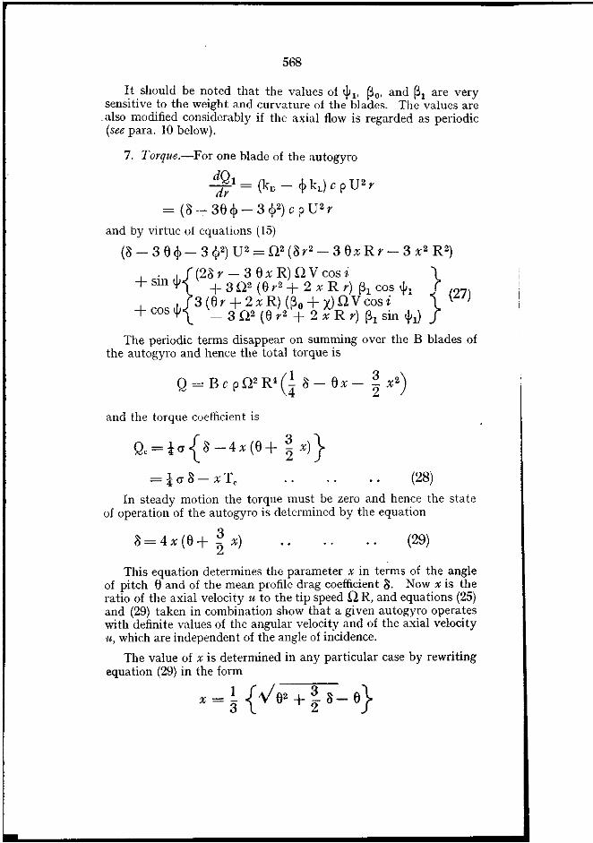
7. Torque.-For one blade of the autogyro

~~l = (kD - q,kL) C PU2 r

= (Il - 36 q, - 3 q,2) C PU2 r

and by virtue of equations (15)

(Il - 3 6 q, - 3 q,2) U2 = fP (Ilr 2 - 3 6x R r - 3 x2 R2)

. ",{(2Ilr-36XR)QVCOSi ')+sm'!' +3Q2(6r2+2xRr)~lCOs(h}i'

+,I, 3(6r+2xR)(~o+X)QVcosi (27)

COS'!' _ 3 Q2 (6 r 2 + 2 x R r) ~l sin <)il)

The periodic terms disappear on summing over the B blades ofthe autogyro and hence the total torque is

aud the torque coefficient is

Q,=lcr{Il-4x(6+ ~ X)}=tcrll-xT, (28)

In steady motion the torque must be zero and hence the stateof operation of the autogyro is determined by the equation

1l=4x(6+ ~ x) (29)

This equation determines the parameter x in terms of the angleof pitch eand of the mean profile drag coefficient /). Now x is theratio of the axial velocity u to the tip speed Q R, and equations (25)and (29) taken in combination show that a given autogyro operateswith definite values of the angular velocity and of the axial velocityu, which are independent of the angle of incidence.

The value of x is determined in any particular case by rewritingequation (29) in the form

x=1 {V62+~/)-6}

,,i

,i\,I;f.

tI\!iI

IIII,

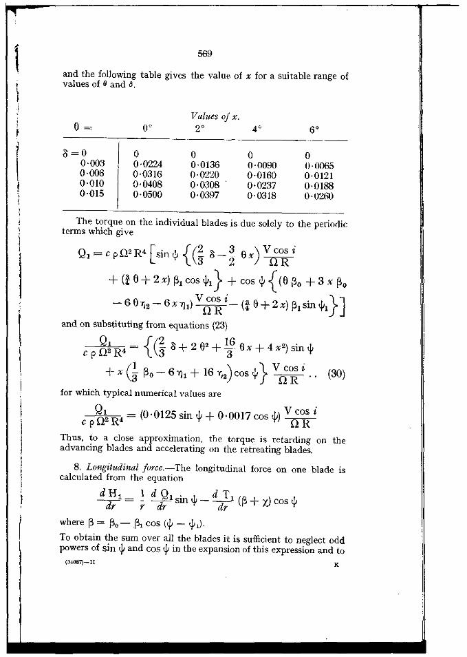
569

and the following table gives the value of x for a suitable range ofvalues of 9 and a.

Values oj x_6= 0° 2° 4° 6°

1)=0 0 0 0 00-003 0-0224 0-0136 0-0090 0-00650-006 0-0316 0-0220 0-0160 0-01210-010 0-0408 0-0308 0·0237 0·01880·015 0-0500 0·0397 0·0318 0-0260

The torque on the individual blades is due solely to the perioclicterms which give

Ql = C P0 2R4 [sin tjJ {(i l) - g6 x) V~~ i

+ (! 6 + 2 x) ~1 cos <)il} + cos <)i {(6 ~o + 3 x ~o

" 6 V cosin. .I.}]- 6 v lJ2 - x lJ1) 0 R (! v + 2 x) ~1 SID 'fl

and on substituting from equations (23)

Ql ={(~l)+262+16ex+4X2)Sin<)ic p 0 2 R4 3 3

( 1 6) .f.} V cos i+ x 3" ~o - 6lJl + 1 lJ2 cos 'f 0 R -. (30)

for which typical numerical values are

c p%~ R4 = (0 ·0125 sin <)i + 0·0017 cos <)i) V~~ i

Thus, to a close approximation. the torque is retarding on theadvancing blades and accelerating on the retreating blades.

8. Longitudinal Jorce_-The longitudinal force on one blade iscalculated from the equation

dH 1 d Q _ d T__1 = _ _1 SIll W- _1 (~+ X) cos <)i

dr r dr ' dr

where ~= ~o-~,cos (<)i - tjJ,)_

To obtain the sum over all the blades it is sufficient to neglect oddpowers of sin <)i and cos <)i in the expansion of this expression and to

(34Q87)-1I K

(32)

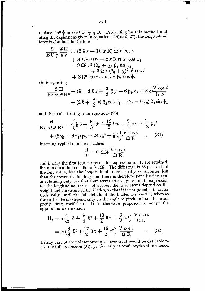
570

replace sin' <Ji or cos' <Ji by ! B. Proceeding by this method andusing the expansions given in equations (19) and (27), the longitudinalforce is obtained in the form

= (2 I> y - 3 II x R) Q V cos i

+ 3 112(() y2 + 2 x R r) ~1 cos IJil- 3 112y2 (~o + X) ~1 sin <Jil

+ 311 r (~o + X)2 V cos i+ 3112 (ll r 2 + x R r) ~1 cos 'h

On integrating2H _ 3 2 Vcosi

Bcp112 RS-(1)-3llx+ 2 ~o -6~o1h+3~) DR

+ (2 II + ~ x) ~1 cos <Jil - (~o - 61)2) ~1 sin IJil

and then substituting from equations (23)

and if only the first four terms of the expression for H are retained,the numerical factor falls to 0·198. The difference is 25 per cent. ofthe full value, but the longitudinal force usually contributes lessthan the thrust to the drag, and there is therefore some justificationin retaining only the first fOUf terms as an approximate expressionfor the longitudinal force. Moreover, the later terms depend on theweight and curvature of the blades, so that it is not possible to assesstheir value until the full details of the blades are known, whereasthe earlier terms depend only on the angle of pitch and on the meanprofile drag coefficient. It is therefore proposed to adopt theapproximate expression

H = (!" + ~ £12 + 13 £1 + ~ 2) V COS i, a 2 0 3 v 2 vX 2 x 11 R

= (~ll2 + 17 II + 15 2) V cos ia 3 2 x 2 x 11R

In any case of special importance, however, it would be desirable touse the full expression (31), particularly at small angles of incidence.

1.571

9. Lateral foree.-The lateral force on one blade is calculatedfrom the equation

d Y 1 = _ .!. d Ql COS <)i _ d T 1 (~+ xl sin <)idr r dr dr

and proceeding as in the case of the longitudinal force

2Be p

.~ -; = 3 n2(6 r2 + 2 X R r) ~1 sin <)il

- 3 (6r + 2xR) (~o + X) nv cosi- 3 (2 6r + X R) (~o+ xl n V cos i+ 3 n2r2 (~o + X) ~1 cos <)il+ 3 n2(6 r2 + X R r) ~1 sin <)il

On integrating

2Y 9 VcosiBcpn2R3=(961)1-26~o-9x~o)nR

. 9+ (~o - 61)2) ~1 cos <)il + (2 6 + 2x) ~1 sin <)il

and then substituting from equations (23)

Be p12 R3 = { 6C52 ~o + ~ 1)1 - 161)2)

_ (.lr.l +24 2)l.Vcosix 2 ,",0 1) j n R (33)

Inserting typical numerical values

-.Y = _ 0.108 V cos iT nR

10. Periodic induced veloeity.-Hitherto the normal inducedvelocity has been assumed to have a constant value v over the wholedisc of the autogyro, but it is evident on physical grounds that theinduced velocity will in fact be greater to the rear and less to the

indicating a lateral force to port, where the blades are retreating,and a magnitude proportional to the forward speed of the autogyro.

Experimentally the lateral force appears to be to port at highspeed and to starboard at low speed. Thus the sense of the variationof the lateral force with speed has been obtained correctly, but thereis a discrepancy in the value at low speeds. To explain this diver­gence it is necessary to abandon the assumption that the axialvelocity u is constant over the whole disc and to consider the effectof a varying induced velocity.

(34087)-11 K2

I

Ii1I

!:;i'II

·1'

'!

:1i!

.......----------------------------------------

572

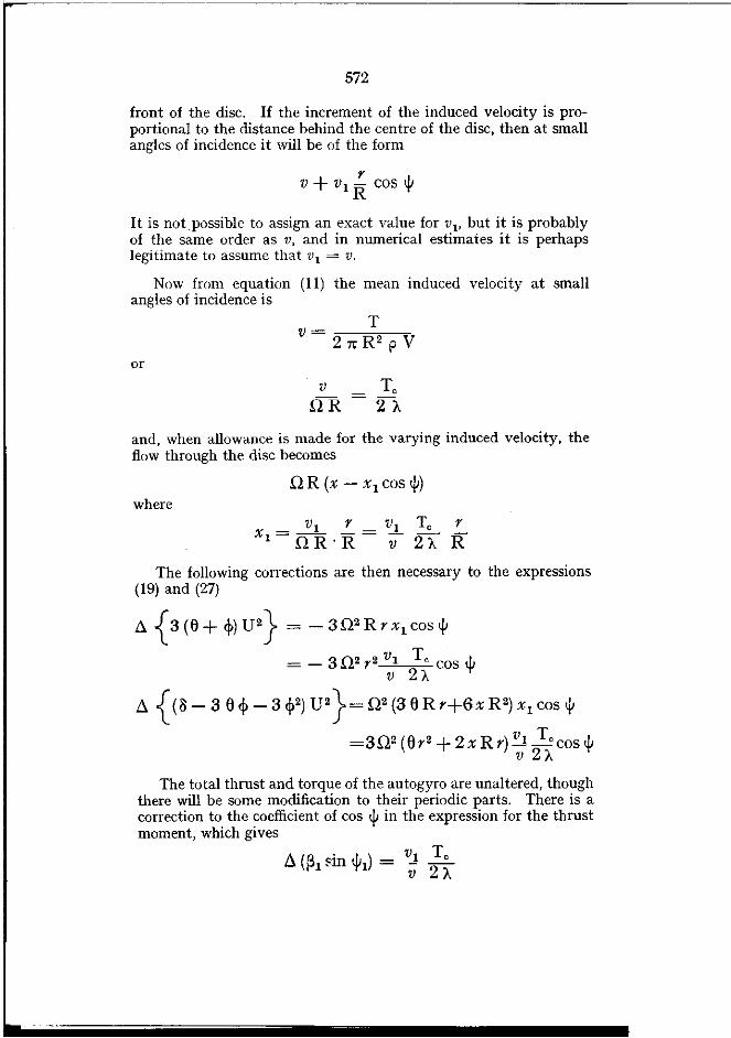
front of the disc. If the increment of the induced velocity is pro­portional to the distance behind the centre of the disc, then at smallangles of incidence it will be of the form

rV + VI R cos <jI

It is notpossible to assign an exact value for v" but it is probablyof the same order as v, and in numerical estimates it is perhapslegitimate to assume that v, = v.

Now from equation (II) the mean induced velocity at smallangles of incidence is

or

and, when allowance is made for the varying induced velocity, theflow through the disc becomes

QR (x - XI cos <jI)where

The following corrections are then necessary to the expressions(19) and (27)

<l {3(ll+ 4»U2} = -3Q2Rrxlcos<jl

= _ 3Q2 r2 VI To cos <jIV 2).

<l {(8 - 3 II 4> - 3 <1>2) U2}= Q2 (3 II Rr+6xR2) XI cos <jI

=3Q2 (llr2+ 2x Rr) VI To cos <jIv 2).

The total thrust and torque of the autogyro are unaltered, thoughthere will be some modification to their periodic parts. There is acorrection to the coefficient of cos <jJ in the expression for the thrustmoment, which gives

~ (~I sin <jI1) = vJ Tov 2).

573

and so the phase angle <p, must be determined from the equation

3 VI T,!~O-3'Y)2+ 16v' 1.2

tan <PI = (34)6+ Ix

which has the typical numerical value0·050tan <PI = 0·54 + ~

The increment of the longitudinal force H is obtained as

d (B ~ p ~~) = - 3 0 2r2 (~o + xl d (~I sin <PI)

+ 302 R r XI (~o + X)which vanishes identically, so that the lift and drag of the autogyroare not altered.

The increment of the lateral force Y is obtained as

d(B~ ~~)=302(26r2+3XRr)d(~lsin<PI)p - 302(6Rr+2xR2)x,

=302(6r2+xRr) VI ToV 2 A

and hence

d ( y ) _ 1 (6 + 3 ) v, T,B c P0 2 R 3 - 4 "2 X V T

or

(35)

This increment indicates a force to starboard, where the blades areadvancing, and a magnitude increasing as the forward speeddecreases. The correction is therefore of the type required toexplain the discrepancy mentioned in the previous paragraph.Nunlerically, however, the correction is not sufficiently large, forwith typical values the lateral force becomes

~ = 0·0034 _ 0.108 AT A

which vanishes when 1.= 0·178. "This value corresponds to anangle of incidence in the neighbourhood of 30°, and the evidenceavailable from full scale flight appears to iudicate that the lateralforce should be to starboard at a moderate angle such as 15°. Thesource of this residual discrepancy may possibly lie in the numericalvalues which have been used to illustrate the general results.

574

11. Lift and drag.-The aerodynamic characteristics of anautogyro depend on the values of three fundamental parameters :-

6 = the angle of pitch of the blades,

Ij = the solidity of the blades,

/) = the mean profile drag coefficient,

and when these values are known, the lift and drag of the autogyroare calculated by means of the following equations :-

/) = 4 x (6 + ~ x)

T e = Ij (6 + ~ x) = ~2 4 x

~ = § 62 + 17 6x + 15 x23 2 2

He = Ij ~ " cos i. . 1 T"smt=x+ "2" ,

V ,,2 cos2 i + x 2

,,' k, = T,cosi - He sin i,,2 k, = Tesin i + H, cosi

(36)

Ij=

The method of using these equations is to calculate, from theknown values of the three fundamental parameters, the values of x,TO' and~. Then, starting with a suitable series of values of "COS i,it is possible to calculate in turn the values of "sin i, i, ", H" k, andk•.

No ambiguity exists as to the value of 6, but if the aerofoilsections are not of symmetrical shape this angle should be measuredfrom the no lift line of the section and not from the chord.

The solidity Ij has been defined as the ratio of the total bladearea to the disc area, but the analysis has been developed on theassumption of blades of constant chord. Thus in the application ofthe equations to the case of blades which are rounded at the tipsand tapered slightly at the root, the value of should he taken to he

Be7tR

where c is the chord length over the greater part of the blade, ratherthan the actual ratio of blade area to disc area.

The value of /) is less certain, since it represents the effectivemean value of the profile drag coefficient. As an aid to the choice

3 (6 + ~ x)

575

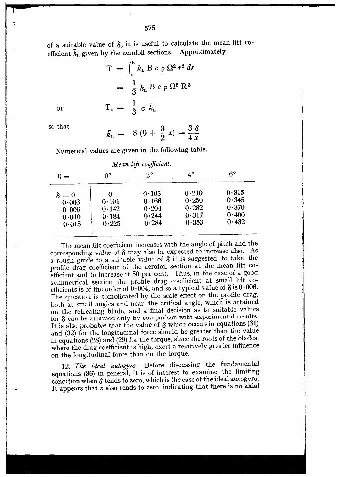
of a suitable value of Il, it is useful to calculate the mean lift co·efficient liL given by the aerofoil sections. Approximately

T = ( kL B c PQZ rZ dr

_ } ilL B c P QZ R 3

1or T, - 3 cr kL

so that

Numerical values are given in the following table.

Mean li]t coefficient.

0' 2'

1l=00·0030·0060·0100·015

o0·1010·1420·1840·225

0·1050·1660·2040·2440·284

0·2100·2500·2820·3170·353

0·3150'3450·3700·4000·432

The mean lift coefficient increases with the angle of pitch and thecorresponding value of amay also be expected to increase also. Asa rongh guide to a suitable value of Il it is suggested to take theprofile drag coefficient of the aerofoil section at the mean lift co­efficient and to increase it 50 per cent. Thus, in the case of a goodsymmetrical section the profile drag coefficient at small lift co­efficients is of the order of 0 '004, and so a typical value of Il is 0·006.The question is complicated by the scale effect on the profile drag,both at small angles and near the critical angle, which is attainedon the retreating blade, and a final decision as to suitable valuesfor /) can be attained only by comparison with experimental results.It is also probable that the value of /) which occurs in equations (31)and (32) for the longitudinal force should be greater than the valuein equations (28) and (29) for the torque, since the roots of the blades,where the drag coefficient is high, exert a relatively greater influenceon the longitudinal force than on the torque.

12. The ideal autogyro -Before discussing the fundamentalequations (36) in general, it is of interest to examine the limitingcondition when I> tends to zero, which is the case of the ideal autogyro.It appears that x also tends to zero, indicating that there is no axial

576

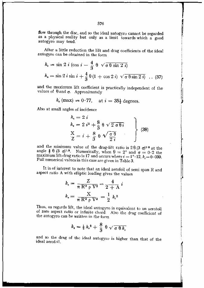
flow through the disc, and so the ideal autogyro cannot be regardedas a physical reality but only as a limit towards which a goodautogyro may tend.

After a little reduction the lift and drag coefficients of the idealautogyro can be obtained in the form

k, = sin 2 i (cos i - } e va esin 2 i)

k. = sin 2 i sin i + ~ e(1 + cos 2 i) Va {) sin 2 i) .. (37)

and the maximum lift coefficient is practically independent of thevalues of !J and a. Approximately

k; (max) = 0'77, at i = 35! degrees.

Also at small angles of incidence

k, = 2 i

k.=2i2+~ev2aei

X=·+~e.vaeZ t 3 2i

and the minimum value of the drag-lift ratio is 2 e(3 a)'" at theangle i !J (3 a)l f3 . Numerically, when e = 2 0 and a = 0·2 themaximum lift-drag ratio is 17 and occurs where i = 10 ·12, k,= 0.039.Full numerical values in this case are given in Table 3.

It is of interest to note that an ideal aerofoil of semi span Randaspect ratio A with elliptic loading gives the values

k, = -----r",Z----."," = 4 i7t R2 P V2 2 + A

X_I k 27t R2 P V2 -2 '

Thus, as regards lift, the ideal autogyro is equivalent to an aerofoilof zero aspect ratio or infinite chord. Also the drag coefficient ofthe autogyro can be written in the form

k. = ! k,2 + ~ ev a ek3 '

and so the drag of the ideal autogyro is higher than that of theideal aerofni1.

III',

I

r~1I,,

IItI

~t

i:~

i

577

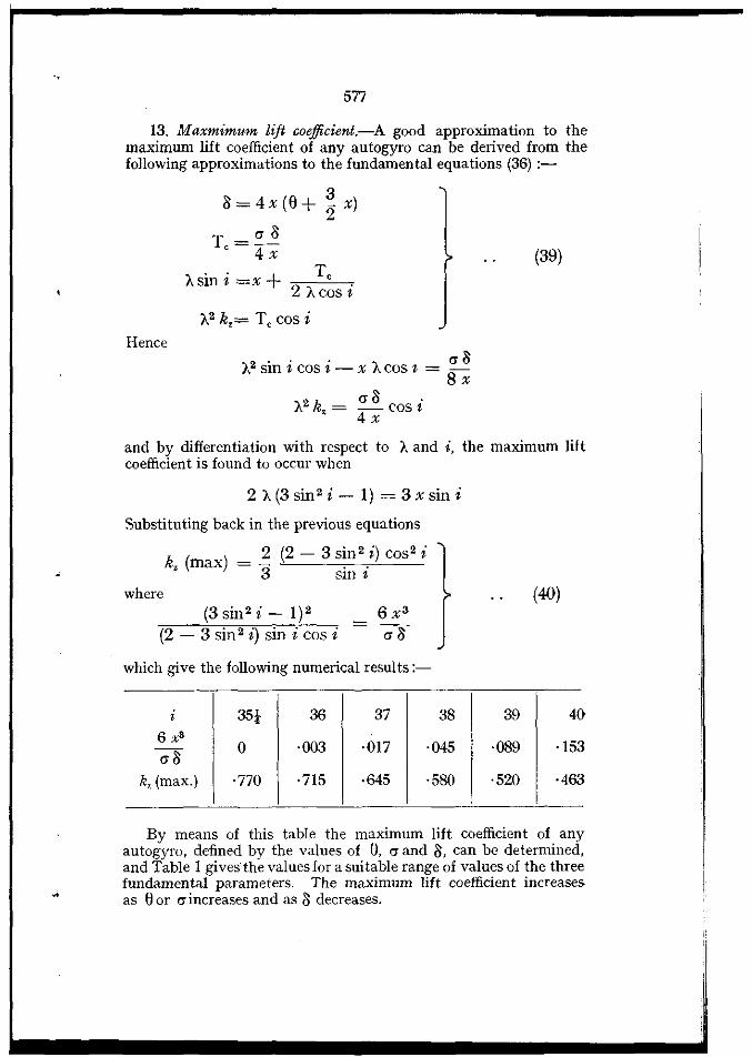
13. Maxmimum lift coefficient.-A good approximation to themaximum lift coefficient of any autogyro can be derived from thefollowing approximations to the fundamental equations (36) :-

Hence

a=4X(e+~X)

T,=~:Asini=x+ T,

2 Acos i

A2 k,= T, cos i

2" " (11)A smtcost-XI\CoSt=Sx

A2k = (11) cosi, 4 x

(39)

and by differentiation with respect to Aand i, the maximum liftcoefficient is found to occur when

2 A(3 sin 2 i-I) = 3 x sin i

Substituting back in the previous equations

k ( )_ 2 (2 - 3 sin 2 i) cos 2 i

zmax-~ o'

3 Sill t

where

(2 - 3 sin 2 i) sin i cos i

(40)

which give the following numerical results:-

i 35! 36 37 38 I 39 406 x·

0 ·003 ·017 ·045 ·089 ·153(11)

k, (max.) ·770 ·715 ·645 ·580 ·520 ·463

By means of this table the maximum lift coefficient of anyautogyro, defined by the values of lJ, (1 and I), can be determined,and Table 1 gives the values for a suitable range of values of the threefundamental parameters. The maximum lift coefficient increasesas lJ or (1 increases and as I) decreases.

578

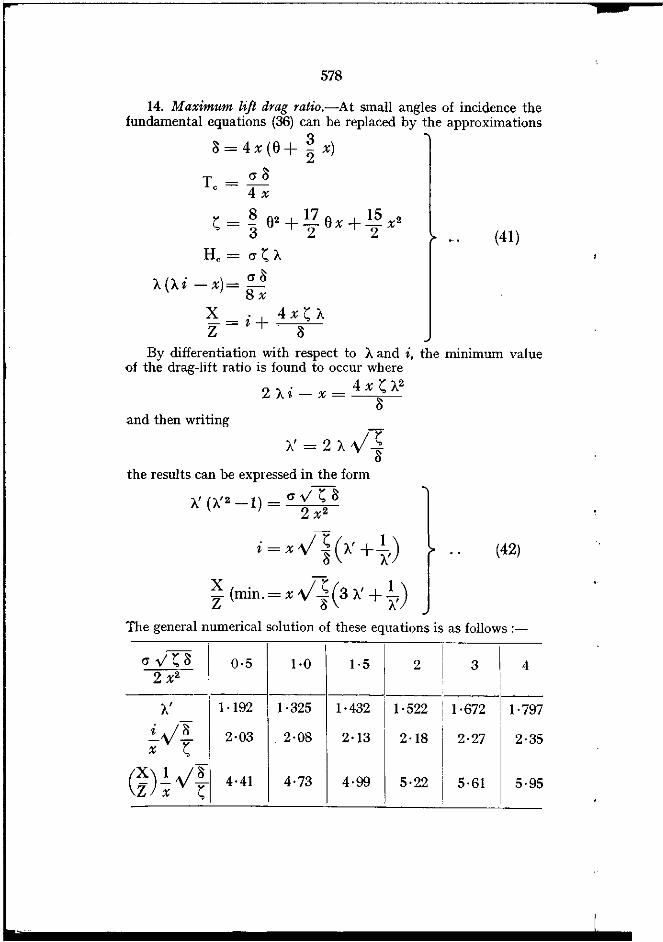
14. Maximum lift drag ratio.-At small angles of incidence thefundamental equations (36) can be replaced by the approximations

3=4x(6+ ~ x)

T = cr 3, 4 x

(41)y = ~ 62 + 17 6x + 15 x2.. 3 2 2

H, = cr~A

A(Ai -x)= cr38x

X=i+ 4xOZ a

By differentiation witb respect to Aand i, the minimum valueof the drag-lift ratio is found to occur where

2 Ai _ x = 4 x ~ 1.2

3and tben writing

the results can be expressed in the form

X (1.'2 -1) = cr vU2 x 2

(42)

The general numerical solution of these equations is as follows :-

5

5

cr V ~ 3 0·5 1·0 1·5 I 2 3 I 42 x2

II

I,

A' 1·192 1·325 1·432 I 1·522 1·672 I 1·797

.£,y3 I I

2·03 2·08 2·13 2·18 2·27 2·3x ~

(~)~,y3 4·41 4·73 4·99 5·22 5·61 5·9Z x ~ I

-.

.,

579

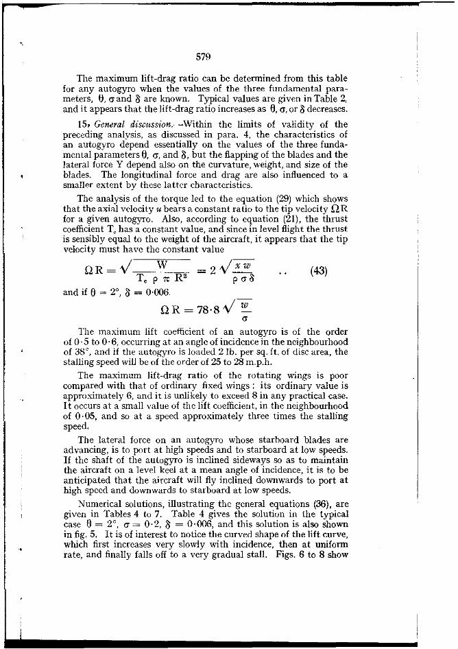
The maximum lift-drag ratio can be determined from this tablefor any autogyro when the values of the three fundamental para­meters, lJ, cr and /) are known. Typical values are given in Table 2,and it appears that the lift-drag ratio increases as lJ, cr, or /) decreases.

15, General discussion.-Within the limits of validity of thepreceding analysis, as discussed in para. 4, the characteristics ofan autogyro depend essentially on the values of the three funda­mental parameters lJ, cr, and /), but the flapping of the blades and thelateral force Y depend also on the curvature, weight, and size of theblades. The longitudinal force and drag are also influenced to asmaller extent by these lattcr characteristics.

The analysis of the torque led to the equation (29) which showsthat the axial velocity u bears a constant ratio to the tip velocity QRfor a given autogyro. Also, according to equation (21), the thrustcoefficient To has a constant value, and since in level flight the thrustis sensibly equal to the weight of the aircraft, it appears that the tipvelocity must have the constant value

Q R = V w = 2 V x w (43)T, p 7t R2 P cr /)

and if e = 2°, /) = 0·006

QR=78'8V W

crThe maximum lift coefficient of an autogyro is of tbe order

of 0·5 to 0,6, occurring at an angle of incidence in the neighbourhoodof 38', and if the autogyro is loaded 21h. per sq. ft. of disc area, thestalling speed will be of the order of 25 to 28 m.p.h.

The maximum lift-drag ratio of the rotating wings is poorcompared with that of ordinary fixed wings: its ordinary value isapproximately 6, and it is unlikely to exceed 8 in any practical case.I t occurs at a small value of the lift coefficient, in the neighbourhoodof 0·05, and so at a speed approximately three times the stallingspeed.

The lateral force on an autogyro whose starboard blades areadvancing, is to port at high speeds and to starboard at low speeds.If the shaft of the autogyro is inelined sideways so as to maintainthe aircraft on a level keel at a mean angle of incidence, it is to beanticipated that the aircraft will fly inclined downwards to port athigh speed and downwards to starboard at low speeds.

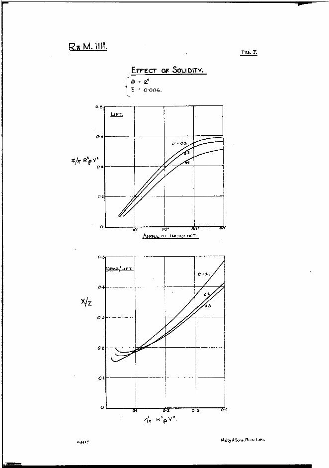
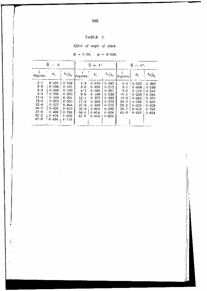
Numerical solutions, illustrating the general equations (36), aregiven in Tables 4 to 7. Table 4 gives the solution in the typicalcase II = 2', cr = 0·2, /) = 0,006, and this solution is also shownin fig. 5. It is of interest to notice the curved shape of the lift curve,which first increases very slowly with incidence, then at uniformrate, and finally falls off to a very gradual stall. Figs. 6 to 8 show

-----------~-~-~~------~--......---r

580

respectively the effect of variation of the profile drag, solidity andangle of pitch. It is desirable that the profile drag should be as lowas possible, a solidity of 0·2 represents a good mean condition buta lower solidity is advantageous for high speed, and an angle ofpitch of 2° is probably the best for the ordinary range of flying speeds.

A discussion of the best conditions for maximum speed 'and ofthe possiblity of vertical descent is given in the appendices. Theimportant conclusion is reached that as the maximum speed ofa gyroplane is increased, the loading must also be increased in orderto maintain a sufficient ratio of tip speed to forward speed, and thereis a corresponding increase of the stalling speed. In the typical case(j = 2°, cr = 0,02, a = 0,006, the values are;-

Maximum speed 85 150 200 m.p.h.Loading (W/7tR') 2·0 6·2 11·0 lb./sq. ft.Stalling speed ... 261 26} 62 m.p.h.

Thus the principal merit of a gyroplane, its low landing speed,inevitably disappears when high speed of level flight is required,and there remains only Ule absence of a sudden stall to counter­balance the very poor efficiency as compared with an aeroplane.

,

581

APPENDIX I.

THE ENERGY LOSSES OF AN AUTOGYRO.

The theory of the autogyro, as given in the main body of the report isdeveloped by considering the aerodynamic forces on the rotating blades. The·theory necessarily involves certain assumptions and approximations. whichunfortunately become less accurate at small angles of incidence and introducesome uncertainty in the determination of the maximum lift-drag ratio. Anattempt has, therefore. been made to analyse the energy account of an auto­gyro in order to provide an independent check on the previous results. Thisanalysis gives an upper limit only to the possible lift-drag ratio since it isnot possible to evaluate fully every possible source of loss of energy. Forsimplicity also the analysis has been confined to small angles of incidence,i.e. to the region where the results of the previous theory are most likely tobe in error.

Two main sources of loss of energy are considered, due respectively to theinduced velocity caused by the thrust and to the profile drag of the blades.An additional source of loss of energy is the periodic distribution of thrustover the disc of the windmill but no simple method has been found of estimat­ing its magnitude.

The analysis assumes the angle of incidence i to be small. and hence it islegitimate to replace cos i hy unity and to regard the lift Z as identicalwith the thrust T. If E is the loss of energy in unit time, the drag X of thewindmill is determined by the equation

XV=Eand the drag-lift ratio of the windmill is ootained as

X EZ - VT

The thrust of the windmill causes an induced velocity v and a correspond­ing loss of energy Tv. The induced velocity will be assumed to have a constantvalue over the disc of the windmill and to be given by the equation

(a)

(b)

as in the previous analysis. The velocity V' in this equation is the resultantof V and v, and for small angles of incidence it is sufficiently accurate totake V' = V. The element of drag corresponding to the induced velocity v isthen calculated simply as

X 1 _ V _ TZ - V - -2 7t R· PV· -

The energy loss due to the drag of the blades will be calculated on theassumption of a mean profile drag coefficient afor the whole of the blades.As a first approximation also, the velocity of the air relative to a typicalelement of the blade at angle ~ from the downwind position is(Qr + V sin ~) and the corresponding loss of energy is

E = L rae p (11 r + V sin IW dr

582

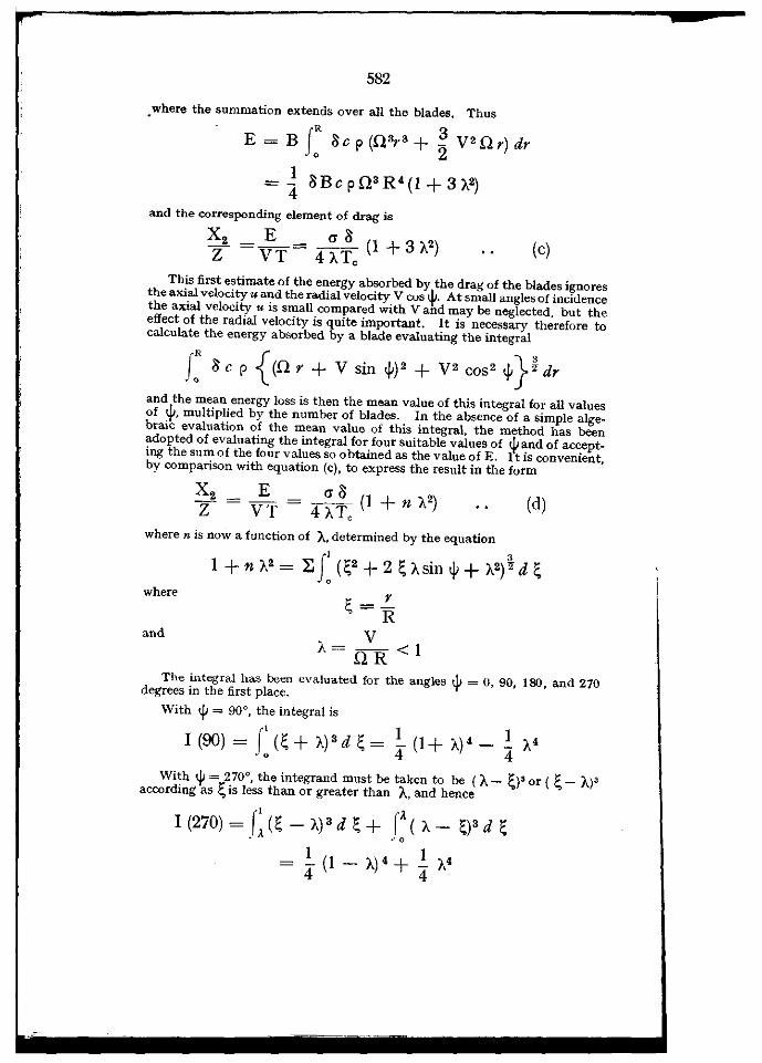
.where the summation extends over all the blades. Thus

fR 3

E = Boil c p (Q3r 3 + 2 V2 Q r) dr

=] ilBcpQ3R4(1+3A2)4

and the corresponding element of drag is

X 2 =~= ~i- (1 + 31.2)Z VT 4ATc

(c)

This first estimate of the energy absorbed by the drag of the blades ignoresthe axial velocity u and the radial velocity V cos~. At small angles of incidencethe axial velocity u is small compared with V and may be neglected, but theeffect of the radial velocity is quite important. It is necessary therefore tocalculate the energy absorbed by a blade evaluating the integral

( il c p {(Q r + V sin </J) 2 + V2 COS 2 </J} l dr

and the mean energy loss is then the mean value of this integral for all valuesof ~,multipliedby the number of blades. In the absence of a simple alge­braic evaluation of the mean value of this integral, the method has beenadopted of eValuating the integral for four suitable values of ~ and of accept­ing the sum of the four values so 0 btained as the value of E. 1t is convenient,by comparison with equation (c), to express the result in the form

(d)

and

where

where n is now a function of A, determined by the equation

1 + n 1.2 = ~ J: (~2 + 2 ~ Asin ~ + 1.2) ~ d ~

~ r-RV

A=QR<1

The integral has been evaluated for the angles ~ = O. 90, 180, and 270degrees in the first place.

With 'iJ = 90°, the integral is

I(90)=fl(~+A)3d~= !-(I+A)4-! 1.4° 4 4

With <jJ = 270°, the integrand must be taken to be (A _ ~)' or ( ~ _ A)3according as ~ is less than or greater than A, and hence

I (270) = J: (~ - A) 3 d ~ + 1:(A- ~)3 d ~

- !- (1 - A) 4 + .!. 1.44 4

583

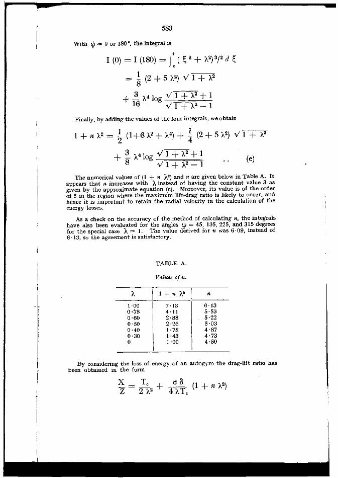
With t = 0 or lSO°, the integral is

I (0) = I (180) = f: (~ 2 + )..2) 3/2 Ii ~

= ! (2 + 5 )..2) V 1 + )..28

+ 1. )..4 log VI + )..2 + 116 V 1+ )..2 - 1

Finally. by adding the values of the four integrals, we obtain

1 + n )..2 = ~. (1+6)..2 + )..4) + i (2 + 5 )..2) VI + )..2

+ ~ A410g VI + )..2 + 1 (e)8 VI +)..2-1

The numerical values of (1 + n ).,2) and n are given below in Table A. Itappears that n increases with A instead of having the constant value 3 asgiven by the approximate equation (c). Moreover, its value is of the orderof 5 in the region where the maximum lift-drag ratio is likely to occur, andhence it is important to retain the radial velocity in the calculation of theenergy losses.

As a check on the accuracy of the method of calculating n, the integralshave also been evaluated for the angles :Ji = 45, 135, 225, and 315 degreesfor the special case A = 1. The value derived for n was 6,09, instead of6·13, so the agreement is satisfactory.

TABLE A.

Values of n.

).. 1+ n ).., n

1·00 7·]3 6·130-75 4'11 5·530·60 2'88 5·220·50 2·26 5·030·40 ],78 4'870·30 ],43 4'730 1·00 4·50

By considering the loss of energy of an autogyro the drag-lift ratio hasbeen obtained in the form

584

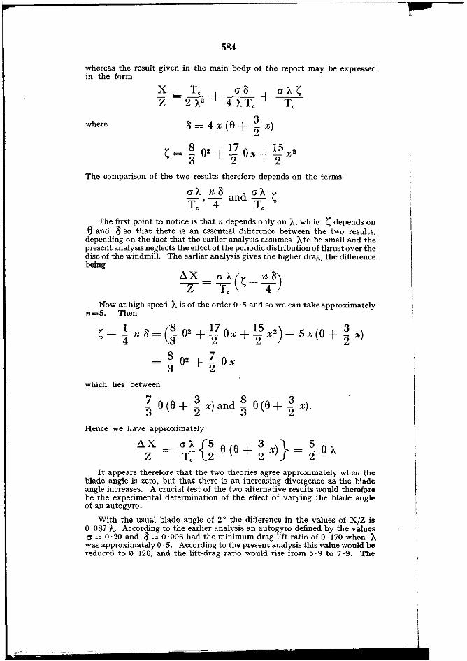
whereas the result given in the main body of the report may be expressedin the form

where

x _ 'I, + cr a + cr" ~Z - 2 ,,2 4 " T, ----r:-

a= 4x (6 + ~ x)

~= ~ 62 + 17 6x+ 15 x23 2 2

The comparison of the two results therefore depends on the terms

The first point to notice is that n depends only on A. while ~ depends on6 and 8 so that there is an essential difference between the two results,

depending on the fact that the earlier analysis assumes Ato be small and thepresent analysis neglects the effect of the periodic distribution of thrust over thedisc of the windmill. The earlier analysis gives the higher drag, the differencebeing

Now at high speed A is of the order O· 5 and so we can take approximatelyn=5. Then

~ - ! n a= (~ 62 + 17 6 x + 15 x 2) - 5 x (6 + ~ x)4 3 2 2 . 2

§ 62 + Z 6 x3 2

which lies between

7 3 8 3"3 6 (6 + '2 x) and 3 6 (6 + '2 x).

Hence we have approximately

~x cr"{53} 5Z = T, 2" 6 (ll + 2 x) = 2 ll"

It appears therefore that the two theories agree approximately when theblade angle is zero, but that there is an increasing divergence as the bladeangle increases. A crucial test of the two alternative results would thereforebe the experimental determination of the effect of varying the blade angleof an autogyro.

With the usual blade angle of 2 0 the difference in the values of X/Z is0·087 A. According to the earlier analysis an autogyro defined by the valuescr = O· 20 and a= 0 '006 had the minimum drag-lift ratio of 0 ·170 when "was approximately O· 5. According to the present analysis this value would bereduced to 0 '126. and the lift-drag ratio would rise from 5·9 to 7·9. The

1--_..---------------------------

585

earlier analysis possibly underestimates the merit of the auto-gyro and thepresent theory certainly overestimates it. The truth must lie somewherebetween the two values given.

The profile drag coefficient of the aerofoil section used on the autogyro isdetermined by model experiments as

This value will be reduced by a factor o· 8 to allow for scale effect, and the meanprofile drag coefficient 0will be assumed to be 50 per cent. greater than thesimple aerofoil value. Then

which gives the value 0' = 0 ·0060 at kL = 0·2 as used in the earlier work.

Now

a= 4x (6 + ~ x)

and the mean lift coefficient is

and hence we derive the equations

X = 0·0225 kL + 0·0036kL

6 = 0·299 kL

_ 0·0054kL

The relationship between 6. kL • x, and Oi5 shown in the following table.

TABLE B.

6

i:,"'I

;(ji

0'2'4'6'

0-1340·2050·2990·397

0-02990-02220-01880·0180

0·00540·00610·00740·0095

The lift-drag ratio can now be expressed in the form

and Table C shows the variation of the lift-drag ratio with the parameter Aand the blade angle 6 for an antogyro of solidity G~ 0·20.

(34087)-II L

586

TABLE C.Lift-drag ratiQ (cr ~ 0 '20).

e~oI

2' ! 4' 6'

" 1·00 4·61 6·07 6·95 6·900·75 5·84 7·46 8·15 8·190·60 6·44 7·96 8·47 8·120'50 6·56 7·84 8·00 7·450·40 6·24 7·07 6·85 6·150·30 5·24 5·50 5·00 4·30

According to these calculations the best blade angle for high speed wouldbe approximately 4°, but unless the ratio of forward speed to tip speed exceeds1/2 there is little advantage over the blade angle 2 0, and the latter is superiorat lower forward speeds.

The analysis of the energy losses of an autogyro has led to a rather morefavourable estimate of the efficiency of an autogyro than was suggested by theprevious analysis, the maximum lift-drag ratio for a typical autogyro risingfrom 6 to 8. It must be remembered. however. that the energy calculationsrepresent an optimum condition which will not be realised, since some sourcesof loss of energy have been neglected.

The chief difference from the previous results is the effect of the bladeangle. According to the earlier analysis the blade angle should be reducedbelow 2 ° for high speed, while according to the present calculations it shouldbe increased to 4 ° or even higher. A useful check on the two alternativemethods of calculation would be provided by the test of a model autogyrowith blade angles 0°,2°, and 4°.

APPENDIX 2.

Conditions for maximum speed.

The aerodynamIc characteristics of an autogyro are detennined by theanalysis of the main report, and in particular, equations (41) represent theconditions at small angles of incidence. It is possible therefore to determinethe thrust horse power Yj P which is required to overcome the drag of therotating blades, and it is found that for any speed of horizontal flight there isan optimum loading w which requires minimum power 1j PjW, or alternativelythe curve of power against speed can be drawn for any given loading.

In horizontal flight the tip velocity of the windmill is, from equation (43),

QR = 2.v," wp cr Il

and the forwanl speed isV="QR

Abo by virtue uf equatiuns (41), the poweI- taken by the windmill is

550'ljP=VXor

550 ~ = V X = V {i + 4x ~_,,}W Z Il

= 2 X .v X w ~ + 2 ~ V2 .vp cr Xpcrll+2pV Ilw

(aj

587

The loading w which requires minimum power at a given fonvard speed, orwhich gives the maximum speed for given power, is determined by the equation

and since

x -vi X w + --"'- = ~ V2 -vi p a Xpaa 2pV aw

w = k, PV2this condition is equivalent to

k 3/2 + 2 X -vi X k = 2 y -vi a X. aa'" a (b)

[0 this case also

550 1) P = V (~k + 4 X -vi X k.)}W 2 ' cra

(c)OR _ 2 -vlXk,----.;r - crT

Equation (a) can be used to determine the power taken by the windmillat any speed V with any loading w, while equations (b) and (c) determine thebest conditions for horizontal flight. The numerical solution for an autogyroe= 2°. 8 = 0 ·006 is given in the following table, which represents theoptimum conditions ;-

cr 0·10 0·15 0,20 0·25 0·30

k, 0·036 0·046 0'054 0'061 0·068

OR2·28 2·12 2·00 1·90 1·82-y

w1·0910" V2 0·84 1·28 1·45 1·61

10' ir~ 2'79 2·95 3·08 3·19 3·30

It has been suggested in the main report that, for efficient working, theratio Q R/V must not fall below the value 2. The optimum conditions forsolidities equal to or less than 0·2 satisfy this condition, but in the case of thehigher solidities it would be necessary to use a slightly heavier loading than theoptimum value.

For the solidity 0·2 the optimum loading is the lightest that can be usedand this loading varies with the speed as follows :-

V ~ 85 150 200 m.p.h.w ~ 2·0 6·2 11·0 Ib./,q.ft.

A reduction of the solidity leads to improved speed of horizontal flightsince the power taken by the windmill is reduced. Also the best loading fallsmore rapidly than the maximum lift coefficient and hence the higher topspeed is accompanied by a lower stalling speed. The limiting condition forthis method of improvement is clearly the impossibility of making very thinblades of large radius and is a matter of structural strength. In any case,however, it appears to be inevitable that the loading and stalling speed mustrise with the top speed of the gyroplane.

(34087)-1 I L 2

588

APPENDIX 3.

Vertical descent.

The problem of the vertical descent of a syroplane is essentially that ofdetermining the drag of a windmill subject to an axial velocity V. Theequations of the main report remain valid with the exception of those whichdefine or involve the axial induced velocity. The velocity of flow tluQugh thedisc u is unaltered and the tip speed of the windmill is given by the equation :-

In order to determine the velocity of descent it is necessary to turn to theordinary airscrew theory. It is customary to write

T = 2 1t R 2 P V2 f= 2 1t R2 P u 2 F

and in the regime in which the windmill is operating the coefficients f and Fare connected by a purely empirical relationship. The value of F is 0 btainedat once as

and if the corresponding empirical value of f is knowD/ the speed V is obtainedfinally from the equation

If the windmill behaved as a parachute of the same disc area, ! would havethe value O· 3, but experimental evidence appears to indicate that the value off may be rather higher and may possibly, as an extreme limit, attain the value0·5. There is no evidence to indicate a value higher than 0 ·5.

Taking! = 0·5 as the highest possible value, the speed of descent becomes

v = 20·5Vwwhich is of the order of 30 f.p.s. or more for ordinary loadings.

A typical value of F, when e= 2°, (J = 0 '2, and a= 0 ·006 is 14 and forvalues of F in this neighbourhood the empirical value of f is given by theequation

In this case, therefore, f = 0·4, and the velocity of descent becomes

It is possible that there may be some cushioning effect on approachingthe ground. but in free descent with a loading of 2 it is improbable that thevelocity is less than 30 I.p.s. and 35 f.p.s. is a more probable figure. It isdoubtful, however, whether the controls of a gyroplane are adequate to holdthe aircraft in a steady vertical descent.

589

APPENDIX 4.

Notaticm.

angular velocity about shaft.

angular position of blade.

angular rotation of blade about its hinge

~ = ~o - ~, cos (<jJ-'j!,).angle of incidence of autogyro.fonvard speed.axial induced velocity.resultant of V and v.axial velocity through disc.resultant velocity relative to blade element.inclination of velocity U (Fig. 4).

total weight.W

1tR'thrust.longitudinal force.drag.lateral force.lift.torque.

number of blades.angle of pitch.extreme radius.radius to blade element.chord of blade element.ordinate from base line (Fig. 2).slope of blade element.weight of one blade.weight moment about hinge.moment and product of inertia.

w

THXYZQ

iVvV'=u =u=<jJ=

w

Q<.)1=~=

T, T/1tR' P Q, R', etc.h, X/1tR' PV', etc.

kL, kD = lift and drag coefficients of blade element.8 = mean profile drag coefficient.

cr = :~ (the solidity).

VA = Q R

Coefficients.

Forces.

Genera! motion.

Dimensions uf blades.Ba=

RrchX

W,G,

II' J.1Motion of blades

ux = QR

8' 17 15~ ="3 a + 2' ax + 2" x'

~. 1)1> 1)2 = coefficients of the blade curvature, equations (6).

C:, ~1' [L!! = coefficients of the blade density, equations (7).

,,!