BarcelonaEconomicsWorkingPaperSeries

WorkingPapernº369

A General Framework for Growth Models with Non-Competitive Labor and Product

Markets and Disequilibrium Unemployment

Xavier Raurich

Valeri Sorolla

A General Framework for Growth Models with Non

Competitive Labor and Product Markets and

Disequilibrium Unemployment

Xavier Raurich �

Universitat de Barcelona and CREP

Valeri Sorolla y

Universitat Autònoma de Barcelona

December 19, 2008

Abstract

In this paper we derive the general framework for growth models with non competitive

labor and output markets and disequilibrium unemployment. For the three standard

ways of generating savings, the framework makes clear how capital growth depends on

employment and employment on the stock of capital and how both variables depend on the

real wage and the markup. Then we analyze the long run relationship between growth and

unemployment for some standard wage setting rules: constant real wages, rules that imply

a constant unemployment rate and rules with inertia on wages and labor incomes, paying

special attention to the neoclassical production function with in�nite horizon consumers,

the Ramsey model (the canonical model of growth) with unemployment.

Keywords: Disequilibrium Unemployment, Growth, Wage Setting.

JEL number: E24, O41.

�Raurich is grateful to the Spanish Ministry of Education for �nancial support through grant SEJ2006-05441.yDepartament d�Economia i d�Història Econòmica, Universitat Autònoma de Barcelona, Edi�ci B - Campus

UAB, 08193 Bellaterra, Spain; tel.: +34-93.581.27.28; fax: +34-93.581.20.12; e-mail: valeri.sorolla@uab.cat.Corresponding author. Sorolla is grateful to the Spanish Ministry of Education for �nancial support throughgrant SEJ2006-03879. We would like to thank Juan Carlos Conesa, Stefano Gnocchi and Howard Petith fortheir helpful comments.

1. Introduction

If you ask to an economist what is the long run relationship between growth and unemployment

the most probably answer that you will get is that there is no relationship, meaning that the

variables that determine the rate of unemployment are di¤erent that the ones that determine the

rate of growth. On the contrary, for the short run you can frequently �nd economic institutions

recommending wage moderation since, according to them, a higher wage is going to increase

unemployment and decrease capital accumulation and thus lower growth and employment in

the future. The purpose of this paper is to set out a general frame of a model in which there is

wage setting and disequilibrium unemployment and into which is inserted the three usual ways

of generating a savings function: a constant savings ratio (ECSR), an in�nite horizon (IH) and

overlapping generations (OLG); and then use this framework to analyze the e¤ect of wages on

growth and employment and the long run behavior of these variables for di¤erent wage setting

rules and production functions.

As Aricó (2003) notes in his survey about growth and unemployment, there are not many

papers with models that combine both topics. Models that deal with growth and unemployment

can be divided according to how unemployment is generated.

On the one hand, we have the disequilibrium approach, the non-Walrasian labor market

structure, where there is unemployment because the wage set by somebody implies excess

supply of labor in a labor market without frictions. This somebody may be unions, and then

we have the union monopoly model (Mc Donald and Solow (1981)), or �rms, and then we

have the e¢ ciency wage model (Solow (1979)). On the other hand, there is the equilibrium

unemployment approach where there are frictions in the labor market due to matching problems

and the unemployment rate is the one that equilibrates �ows into and out of the labor market.

We follow the disequilibrium approach because it is the natural framework for highlighting the

e¤ect of wage setting and markups on both unemployment and capital accumulation. Moreover,

this approach facilitates the comparison with the standard growth models with full employment

that one can �nd in an advanced textbook of economic growth (Sala-i-Martín (2000), Barro

and Sala-i-Martín (2003), Romer (2007)).

In the equilibrium unemployment literature, Pissarides (1990) set out the �rst model with

growth and frictional unemployment where growth is an exogenous variable. Pissarides pos-

tulates a positive e¤ect of total factor productivity (TFP) growth (technological progress) on

employment via the capitalization e¤ect. Aghion and Howitt (1998 pp. 127) explain the cap-

italization e¤ect as follows �an increase in growth raises the rate at which the returns for

creating a plant (or a �rm) will grow and hence increases the capitalized value of those returns,

thereby encouraging more entry by new plants and therefore more job creation�. Following this

idea several authors (Aghion and Howitt (1994 and 1998), Mortensen and Pissarides (1988),

Mortensen (2005)) endogenize the TFP growth in the matching model by introducing Aghion

and Howitt´s model of creative destruction that also generates a negative e¤ect on employment

due to the creative destruction e¤ect of growth. Bean and Pissarides (1993) with an overlapping

generations model (OLG) without either the capitalization or the creative destruction e¤ect an-

alyze the case where employment a¤ects labor income and, hence, growth and Eriksson (1997)

2

does the same with an in�nite horizon model.

The existence of growth due to capital accumulation implies that growth depends on em-

ployment and employment depends on growth, this complicates the basic static models used in

the disequilibrium approach because of the e¤ect of wages on capital and future employment.

Van der Ploeg (1987) and Sorolla (1995) analyze the solution of the program of a union that

takes into account this dynamic e¤ect. Models with growth and disequilibrium unemployment

use, then, simplifying assumptions on production functions and wage setting rules that make

the models tractable.

The �rst contribution of the paper to this literature is to derive in a transparent way the

general set up that illustrates the relationship between growth and unemployment and its

dependence on wages and mark ups for the three standard ways of deriving savings. Secondly

we analyze the relationship between growth and unemployment for the AK production function

and the wage setting rules that appear in some papers, extending the analysis to the neoclassical

production function. We pay special attention to the in�nite horizon consumers case, the

Ramsey model (the canonical model of growth) with unemployment, that is not studied in

these papers. The analysis makes clear in which cases there is no relationship between growth

and unemployment in the long run.

The general framework of this paper includes, as special cases, the set ups that have been

used in the following papers: Raurich, Sala and Sorolla (2006) has an IH model with wage

inertia due to past labor income and an AK production function, where di¤erent types of �scal

policy generate multiplicity of equilibria and, then, hysteresis. Raurich and Sorolla (2003a)

employs an IH model with a wage setting rule that implies a constant unemployment rate

and a positive externality on TFP of the ratio of public to private capital, where the e¤ect

of taxes on growth and unemployment is analyzed. Raurich and Sorolla (2003b) makes use

of an OLG model with wage inertia and an AK production function, where we show that

wage inertia implies that growth has a permanent e¤ect on long run unemployment and the

e¤ect of di¤erent taxes on growth and unemployment is analyzed . Sorolla (1995) sets out a

�nite horizon model with a Leontie¤ production function, where the e¤ect of a more proworker

government on employment is analyzed. Sorolla (2000) employs an OLG model with wage

inertia and neoclassical production function, where the conditions for convergence to an steady

state and the e¤ect of a more proworker government on long run employment and growth are

analyzed. Daveri and Tabellini (2000) use an OLG model in order to analyze the e¤ect of

taxes on both variables with a particular wage setting rule that eliminates the e¤ect of growth

on employment and the same do Domenech and García (2008), with a IH model, in a more

complex framework with a detailed structure of taxes and social bene�ts. They use a general

production function that, for the AK case, we show, that employment does not have e¤ect on

growth. In this case, in order to have a positive e¤ect of employment on growth, they introduce

a positive externality of capital per capita, an addition that was criticized by Sala-i-Martin

(2000), section 2.8.

Papers with wage setting rules more complex that the ones presented in this paper are:

Daveri and Ma¤ezzoli (2000) where they also analyze the e¤ect of taxes on long run growth

and unemployment using and in�nite horizon model with a CES production function where

3

the accumulation of knowledge is a by-product of being employed, which implies that growth

depends on employment; Kaas and von Thadden (2003) that, using an OLG model with a CES

production function, study how the elasticity of substitution between labor and capital a¤ects

the dynamics of growth and unemployment; and Galí (1996b) that presents an in�nite horizon

model with imperfect competition in the product market and labor choice. Models of growth

with disequilibrium in the labor market have also been used in the real business cycle literature

to analyze the e¤ect of real shocks on unemployment �uctuations (Galí (1995), Benassy (1997)

and Ma¤ezzoli (2001)).

The rest of the paper is organized as follows. Section 2 presents the �rm behavior. Section 3

analyzes consumer behavior and the fundamental equations for the IH model when there is wage

setting and unemployment. Section 4 presents, the special case where growth does not depend

on wages and employment. Section 5 describes the constant real wage case. Section 6 the

special wage setting rules that imply a constant employment rate and, hence, that employment

does not depend on growth. Section 7 adds inertia on wages and labor income to the rules of

Section 6 and Section 8 concludes with a summary of the main results. Appendix 1 presents

the fundamental equations for the ECSR and OLG models and appendix 2 the special case

where growth does not depend on wages and employment for the ECSR and OLG models.

2. Firms

2.1. Price Taking Firms

We assume the neoclassical production function:

Yt = F (Kt; Lt),

with constant returns to scale with respect toK and L, FK > 0, FL > 0, FKK < 0, FLL < 0 and

the Inada conditions: LimK!0FK = 1, LimK!1FK = 0, LimL!0FL = 1, LimL!1FL = 0.

The production function in terms of output per worker or unit of labor, YLt� yt, and capital

per worker or the capital labor ratio, KLt� kt, that is, in intensive form, is:

yt = f(kt),

where f 0 > 0 and f��< 0. The �rm is price taker and maximizes pro�ts:

F (Kt; Lt)� !tLt � (rt + �)Kt,

where !t is the real wage, rt the interest rate and � the constant depreciation rate, 0 5 � 5 1.As usual, the conditions for the e¢ cient use of factors and zero pro�ts are:

FL(Kt; Lt) = !t,

and

FK(Kt; Lt) = rt + �,

4

expressions that we can rewrite in intensive form as:

f(kt)� ktf 0(kt) = !t, (2.1)

and

f 0(kt) = rt + �. (2.2)

Conditions (2.1) and (2.2) give the combinations between !t, rt and kt such that factors are

e¢ ciently used and pro�ts are zero and, then, capital and labor demand are any quantity that

satis�es kt1.

We assume that labor supply is equal to population, Nt, that growths at a constant rate n.

In models with unemployment and population growth, we also need to rewrite the production

function in terms of output per capita YtNt� yt, capital per capita Kt

Nt� kt and the employment

rate LtNt� lt. Because of the constant returns to scale assumption, we rewrite the production

function as:

YtNt= F (

Kt

Nt;LtNt),

that is:

yt = F (kt; lt).

We also rewrite the conditions for the e¢ cient use of factors and zero pro�ts as:

Fl(kt; lt) = !t, (2.3)

and

Fk(kt; lt) = rt + �. (2.4)

and we rewrite the zero pro�ts condition as:

yt = F (kt; lt) = (rt + �)kt + !tlt, (2.5)

and, it is obvious that:

FK(Kt; Lt) = f0(kt) = Fk(kt; lt). (2.6)

The main characteristic of models with wage setting is that the real wage !t is set by

somebody2 and, then, from (2.1) we get the capital labor ratio function:

kt = ~k(!t), (2.7)

1See Barro and Sala-i-Martín Section 2.2 for the precise derivation of the conditions and a more extensivediscussion on this point.

2Thus, we are in economies where labor contracts include indexation of wages.

5

where ~k0 > 0. From (2.7) we get the "labor demand" function:

Ldt = ~L(!t; Kdt ) =

Kdt

~k(!t), (2.8)

where ~L! < 0 and ~LKd > 0:

Also from (2.2) and (2.7) we get the interest rate function (the interest rate-wage frontier):

rt = ~r(!t) = f0(~k(!t))� � (2.9)

that gives, for a given wage, the interest rate that implies zero pro�ts. It is easy to check that

r0 < 0, which means that, if the wage increases, the interest rate must decrease in order to have

zero pro�ts. Of course, if the interest rate is higher that the one given by this function, then

pro�ts are negative and then the demands for labor and capital are zero. If it is lower, then

pro�ts are positive and capital and labor demand are in�nite. In textbook macroeconomic

models, with the stock of capital given and a keynesian investment function, it turns out that

the relation between the real wage and the real interest rate is positive, this is because an

increase in the wage implies less employment and less production and, if we have equilibrium in

the goods market (the IS equation), in order for demand to fall, the interest rate must increase.

In models with wage setting in general there is no equilibrium in all markets if the wage is

di¤erent from the competitive wage. It is only assumed that the interest rate adjusts in order

to have equilibrium in one market. This is only possible if the zero pro�t condition holds, that

is, if the interest rate is given by the interest rate function. In this case, as we have seen,

the labor demand function is, in fact, only a relationship between capital and labor demand.

This property implies that, in models with wage setting, it is the case than one market is not

in equilibrium. Is is easy to see, that either the capital market is in equilibrium and there is

excess supply in the labor market (unemployment) or the labor market is in equilibrium and

there is excess supply in the capital market. We will concentrate on the case where there is

unemployment and the capital market is in equilibrium, this means that the wage that is set

implies that Kdt = K

st = Kt and Lt = Ldt < Nt.

3 Using (2.8), we get the employment function,

Lt, that is:

Lt = Ldt =

~L(!t; Kt) =Kt

~k(!t). (2.10)

Using (2.10) we get the employment rate function:

lt = ~L(!t; kt) =kt~k(!t)

. (2.11)

Writing the production function per capita: yt = F (kt; lt) and taking into account the

employment rate function (2.11) we get:

yt = F (kt;kt~k(!t)

).

3That means that in a concrete model we have to check if this is the case for a given !t.

6

or the output per unit of capital function4:

ytkt= F (1;

1~k(!t)

) = ~f(1

~k(!t)).

Note, from the last function, that if the wage increases then output per unit of capital decreases,

due to the increase in the capital labor ratio, that is, d~f

d!< 0 . As we will see later, this function

plays an important role in some growth models.

Looking at the employment function, (2.10), we see that an increase in the wage implies,

directly, less employment, we call this direct e¤ect of the wage on employment channel 1. We

see also that an increase in capital increases also employment. We interpret this fact saying

that growth a¤ects employment (or employment depends on growth) in the sense that a higher

rate of growth of capital implies more capital and, hence, more employment. In a growth model

with wage setting, the complication arises from the fact that, with equilibrium in the capital

market, there are two indirect channels such that the wage may also a¤ect employment. On

the one hand, by the interest rate function (2.9), a change in the wage may change the interest

rate and this may change consumption and the saving rate, and then, savings, investment and

the supply of capital, if consumption depends on the interest rate. We call this indirect e¤ect

of the wage on employment channel 2. On the other hand, a change in the wage a¤ects directly

and indirectly, changing employment, aggregate labor income, if it a¤ects the interest rate then

also capital income changes. Adding both e¤ects, changes in the wage modify aggregate income

and, then, this may change savings, investment and the supply of capital. We call this indirect

e¤ect of the wage on employment channel 3. When one of these two channels is active we

say, in a general sense, that growth depends on employment (or employment a¤ects growth),

meaning that wages a¤ect the accumulation of capital. In general, in a growth model, we have

that employment depends on growth and growth depends on employment but, depending on

the concrete assumptions made about production functions, households and wage setting, in

some cases, these e¤ects and channels are not active.

2.2. Extension 1: Monopolistic Competition in the goods market

So far we have seen how wages a¤ect employment when �rms are price takers, that is, when

there is perfect competition in the goods market. It is interesting to present the extension for

price setting �rms in order to see that also pro�ts, or markups, a¤ect employment. We introduce

the monopolistic competition set up in a growth model (Galí (1996)) having S sectors with one

�rm i per sector that produces product Yi;t with the production function

Yi;t = F (Ki;t; Li;t),

with the usual properties. The stock of capital is a composite of all produced goods and the

�rm in sector i maximizes the wealth of its shareholders subject to the demand function (see

Galí (1996) for the complete set up). Assuming that the price elasticity of the demand function

4Bentolila and Saint Paul (2003) use the inverse of output per unit of capital, that is capital per unit ofoutput ky =

kF (k;l) =

1f( lk )

in order to compute the labor share.

7

is constant5 and equal to �, we de�ne m � 1(1� 1

�)= 1, as the monopoly degree or the markup,

and in a symmetric equilibrium we get the following two �rst order conditions for the capital

labor ratio for �rm i (see again Galí (1996)):

f(kt)� kf 0(kt) = m!t, (2.12)

and

f 0(kt) = m(rt + �). (2.13)

Thus, we can proceed in the same way that we did in the competitive case, adding the

markup. That is from (2.12) we get the capital labor ratio:

kt = ~k(m!t), (2.14)

where ~k0 > 0. and from the last equation we get the"labor demand" function for sector i:

Ldi;t =~L(m!t; K

di;t) =

Kdi;t

~k(m!t),

where ~Lm! < 0 and ~LKd > 0: Aggregating for all sectors we have the total "labor demand"

function:

Ldt =~L(m!t; K

dt ) =

Kdt

~k(m!t),

where Kdt is the aggregate (composite) stock of capital. Also from (2.13) and (2.14) we get the

interest rate function (the interest rate-wage frontier):

rt = ~r(m!t) =1

mf 0(~k(m!t))� �,

where ~r0 < 0:

The interesting result of this extension is that an increase in market power (in the markup),

has the same potential e¤ects on labor demand as an increase in the wage: it decreases labor

demand directly (channel 1), it decreases the interest rate (channel 2) and it a¤ects aggregate

income by decreasing labor demand and the interest rate and by changing pro�ts (channel 3).

2.3. Extension 2: Exogenous Technological Progress

It is also interesting to examine this extension in order to understand the relationship between

wages and productivity growth. Now we use the production function, with labor-augmenting

technological progress:

Yt = F (Kt; AtLt),

5The complication of the monopolistic competition set up in a growth model arises from the fact that bothconsumers and �rms demand product i due to the demand of capital of each �rm. In principle the priceelasticity of both types of demand may be di¤erent, this is the point of Gali�s paper, and this opens the doorfor multiplicity of equilibria. The assumption that � is constant is the � = � case in Gali´s paper.

8

with constant returns to scale and FK > 0, FAL > 0, FKK < 0, FALAL < 0 and we assume

that _AA= x > 0, that means that there is technological progress. The production function in

terms of output per e¢ ciency unit of labor, YALt

� ye;t, and capital per e¢ cient unit of labor orthe capital e¢ cient labor ratio, K

ALt� ke;t , that is, in intensive form, is:

ye;t = f(ke;t).

The �rm is price taker and maximizes pro�ts:

F (Kt; AtLt)� !tLt � (rt + �)Kt,

where !t is the real wage, rt the interest rate and � the constant depreciation rate, 0 5 � 5 1.As usual, the conditions for pro�t maximization and zero pro�ts are:

FL(Kt; AtLt) =!tAt,

and

FK(Kt; AtLt) = rt + �,

expressions that we can rewrite in intensive form as:

f(ke;t)� ke;tf 0(ke;t) =!tAt, (2.15)

and

f 0(ke;t) = rt + �. (2.16)

It is useful to rewrite the production function in terms of output per e¢ ciency personYtAtNt

� ye;t, capital per e¢ ciency person Kt

AtNt� ke;t and the employment rate lt = Lt

Nt. Because

of the constant returns to scale assumption, we can rewrite the production function as:

YtAtNt

= F (Kt

AtNt; At

LtAtNt

),

that is:

ye;t = F (ke;t; lt).

In this case the �rst order conditions for pro�t maximization and zero pro�ts are:

Fl(ke;t; lt) =!tAt, (2.17)

and

Fke(ke;t; lt) = rt + �. (2.18)

9

We can rewrite the zero pro�ts condition as:

yt = (rt + �)ke;t +!tAtll, (2.19)

and, it is obvious that:

FK(Kt; AtLt) = f0(ke;t) = Fke(ke;t; lt). (2.20)

Now we can proceed in the same way that we did without technical progress. From (2.15)

we get the capital e¤ective labor ratio is

ke;t = ~ke(!tAt), (2.21)

where ~k0e > 0. From (2.21) we get the "labor demand" function:

Ldt =~L(!t; K

dt ) =

Kdt

At~ke(!tAt),

where ~L! < 0 and ~LKd > 0. Assuming equilibrium in the capital market, we get the employment

rate function:

lt = ~L(!t; ke;t) =ke;t~ke(

!tAt). (2.22)

Also from (2.21) and (2.16) we get the interest rate function (the interest rate-wage frontier):

rt = ~r(!tAt) = f 0(~ke(

!tAt))� �.

Now we can discuss the popular idea that in order to have a constant employment rate we

have to link the real wage growth with productivity growth. This result comes from the use of

the Cobb-Douglas production function Yt = AtK�(Lt)1�� with a given level of capital, �K6. In

this case employment is given by:

Lt =

"1� �!tAt

# 1�

�K.

Assuming the stock of capital given, we have: _LtLt= � 1

�( _!t!t� _At

At) so that, in order to have

employment constant, we need !tAtconstant, that is the rate of growth of wages must be equal

to the productivity rate ( _!t!t= x). The popular idea comes from this result.

First remark: if there is population growth then the employment rate is:

lt =1

Nt

"1� �!tAt

# 1�

�K

and then, taking logs and di¤erentiating the employment function with respect to time, we get

6Or Yt = At(Lt)1��, as it is usual in an static model.

10

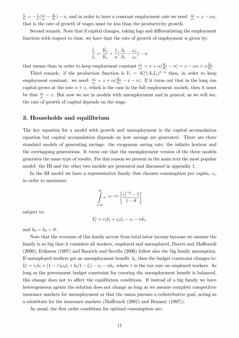
_ltlt= � 1

�( _!t!t� _At

At)� n, and in order to have a constant employment rate we need _!t

!t= x� �n,

that is the rate of growth of wages must be less than the productivity growth.

Second remark: Note that if capital changes, taking logs and di¤erentiating the employment

function with respect to time, we have that the rate of growth of employment is given by:

_ltlt=

_Kt

Kt

+1

�(_AtAt� _!t!t)� n

that means than in order to keep employment constant _!t!t= x+ �(

_Kt

Kt� n) = x� �n+ � _Kt

Kt:

Third remark: if the production function is Yt = K�t (AtLt)

1�� then, in order to keep

employment constant, we need: _!t!t= x + �(

_Kt

Kt� x � n). If it turns out that in the long run

capital grows at the rate n+ x, which is the case in the full employment models, then it must

be that _!t!t= x. But now we are in models with unemployment and in general, as we will see,

the rate of growth of capital depends on the wage.

3. Households and equilibrium

The key equation for a model with growth and unemployment is the capital accumulation

equation but capital accumulation depends on how savings are generated. There are three

standard models of generating savings: the exogenous saving rate, the in�nite horizon and

the overlapping generations. It turns out that the unemployment version of the three models

generates the same type of results. For this reason we present in the main text the most popular

model: the IH and the other two models are presented and discussed in appendix 1.

In the IH model we have a representative family that chooses consumption per capita, ct,

in order to maximize:

1Zt=0

e�(��n)t�c1��t � 11� �

�subject to:

_kst = rtkt + !tlt � ct � nkt.

and k0 = �k0 > 0.

Note that the revenues of this family accrue from total labor income because we assume the

family is so big that it considers all workers, employed and unemployed, Daveri and Ma¤ezzoli

(2000), Eriksson (1997) and Raurich and Sorolla (2006) follow also the big family assumption.

If unemployed workers get an unemployment bene�t, bt, then the budget constraint changes to:_kst = rtkt + (1� �)!tlt + bt(1� lt)� ct � nkt, where � is the tax rate on employed workers. Aslong as the government budget constraint for covering the unemployment bene�t is balanced,

this change does not to a¤ect the equilibrium conditions. If instead of a big family we have

heterogeneous agents the solution does not change as long as we assume complete competitive

insurance markets for unemployment or that the union pursues a redistributive goal, acting as

a substitute for the insurance markets (Ma¤ezzoli (2001) and Benassy (1997)).

As usual, the �rst order conditions for optimal consumption are:

11

_c

c=1

�(rt � �) ,

_kst = rtkt + !tlt � ct � nkt,

limt�!1

�tkst = 0

Note that in this model channel two is active because the interest rate a¤ects the rate of

growth of consumption and channel three is also active because a change in the wage a¤ects

aggregate income, rtkt+!tlt, changing ! and, indirectly, l and r. Assuming equilibrium in the

capital market and using the condition (2.4), and the zero pro�ts condition, (2.5), we get:

_ctct=1

�(FK(kt; lt)� (�+ �)) , (3.1)

_kt = f(kt; lt)� ct � (n+ �)kt. (3.2)

Note that the di¤erence between these equations and the equations of the standard solution

with equilibrium in the labor market, that are:

_ctct

=1

�(f 0(kt)� (�+ �)) ,

_kt = f(kt)� ct � (n+ �)kt;

is in the production function7. Note also that employment a¤ects growth meaning that a higher

level of lt increases the growth of capital.

Dividing by k the second equation, substituting in f 0(kt) = FK(kt; lt) and using the capital

labor ratio function (2.7), we get the fundamental equations of the in�nite horizon model with

wage setting:

c;IH =_ctct=1

�

�f 0(~k(!t))� (�+ �)

�, (3.3)

k;IH =_ktkt= ~f(

1~k(!t)

)� ctkt� (n+ �). (3.4)

Note that, from equation (3.3), an increase in the wage increases the capital labor ratio (de-

creases the interest rate) and then reduces the rate of growth of the optimal consumption per

capita, that is channel 2 is active in this model. On the other hand, from equation (3.4), an

increase in the wage reduces the rate of growth of capital per capita, given ct, via channel 3.

These two channels make the e¤ect of an increase of the wage on the accumulation of capital

ambiguous because of the decrease in consumption via channel 3.

7Again, when the labor market is in equilibrium, kt = kt.

12

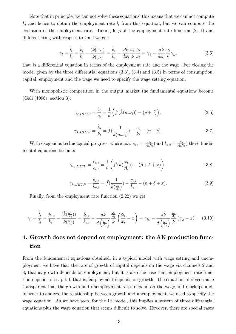
Note that in principle, we can not solve these equations, this means that we can not compute

kt and hence to obtain the employment rate lt from this equation, but we can compute the

evolution of the employment rate. Taking logs of the employment rate function (2.11) and

di¤erentiating with respect to time we get:

l =_ltlt=_ktkt� (

~k _(!t))~k(!t)

=_ktkt� d~k

d!t

!t~k

_!t!t= k �

d~k

d!t

!t~k !: (3.5)

that is a di¤erential equation in terms of the employment rate and the wage. For closing the

model given by the three di¤erential equations (3.3), (3.4) and (3.5) in terms of consumption,

capital, employment and the wage we need to specify the wage setting equation.

With monopolistic competition in the output market the fundamental equations become

(Galí (1996), section 3):

c;IHMP =_ctct=1

�

�f 0(~k(m!t))� (�+ �)

�, (3.6)

k;IHMP =_ktkt= ~f(

1~k(m!t)

)� ctkt� (n+ �). (3.7)

With exogenous technological progress, where now ce;t = CtAtNt

(and ke;t= Kt

AtNt) these funda-

mental equations become:

ce;IHTP =_ce;tce;t

=1

�

�f 0(~k(

!tAt))� (�+ � + x)

�, (3.8)

ke;IHTP =_ke;tke;t

= ~f(1

~k( !tAt))� ce;t

ke;t� (n+ � + x). (3.9)

Finally, from the employment rate function (2.22) we get

l =_ltlt=_ke;tke;t

�(~k _( !t

At))

~k( !tAt)=_ke;tke;t

� d~k

d�!tAt

� !tAt

~k

�_!t!t� x

�= ke �

d~k

d�!tAt

� !tAt

~k( ! � x) : (3.10)

4. Growth does not depend on employment: the AK production func-

tion

From the fundamental equations obtained, in a typical model with wage setting and unem-

ployment we have that the rate of growth of capital depends on the wage via channels 2 and

3, that is, growth depends on employment; but it is also the case that employment rate func-

tion depends on capital, that is, employment depends on growth. The equations derived make

transparent that the growth and unemployment rates depend on the wage and markups and,

in order to analyze the relationship between growth and unemployment, we need to specify the

wage equation. As we have seen, for the IH model, this implies a system of three di¤erential

equations plus the wage equation that seems di¢ cult to solve. However, there are special cases

13

considered in the literature where one of these routes is not active, in these cases the dynamics

are less complex. The �rst special case is when growth does not depend on employment. This

happens when there is an AK production function derived, for example, from a Cobb-Douglas

with capital per unit of labor externalities8: Yt = AKt�L1��t

�Kt1�� (Raurich, Sala and Sorolla

(2006) 9). From (2.1), we get:

(1� �)Ak�t �Kt1�� = !t,

and if the externality is the capital labor ratio �Kt = kt we get:

(1� �)Akt = !t,

or:

kt =!t

A(1� �) ,

and the employment rate function is:

lt =A(1� �)kt

!t. (4.1)

and, then, employment depends on growth.

In this case the fundamental equations of the IH model (3.3) and (3.4) become:

_ctct=1

�(�A� (�+ �)) = �IHAK ,

_ktkt= A� ct

kt� (n+ �).

Because the rate of growth of consumption is constant, one can prove10 that in this set up

the rate of growth of capital is also constant and equal to the consumption growth rate which

implies:

k = �IHAK =

1

�(�A� (�+ �)) ;

which means that growth does not depend on employment. From (4.1) we get:

l = k � ! = �IHAK � !: (4.2)

That is, the growth rate of the employment rate depend on capital growth and wage growth,

and the wage dynamics a¤ects only the dynamics of employment. For the same reason if the

output market is not competitive a change in the markup does not a¤ect growth and the labor

demand is given by:

8Or, alternativelly, the case where the AK function is obtained via productive government expendituresYt = AKt

�L1��t gt1�� (Raurich and Sorolla (2003b)).

9In Raurich and Sorolla (2003a) we also have this function but A depends on average employment and publiccapital.10See, for example, Sala-i-Martín (2000) section 5.3.

14

lt =A(1� �)ktm!t

. (4.3)

As shown in appendix 2, the same kind of result holds for the ECSR and OLG models and

then, when the production function is AK, the rate of growth of capital per capita does not

depend on the wage and the level of wages only a¤ects employment. Summarizing, when the

production function is AK then growth does not depend on wage setting and growth will a¤ect

employment depending on the dynamics of wages, that is, on the wage setting rule.

5. A particular wage setting rule: Constant real wages

If the production function is not AK, then the rate of growth of capital depends on wages and in

order to close the model we need to specify the wage setting rule. The simplest rule is to consider

an exogenous constant real wage, !t = �!. This case is interesting because a constant real wage

is usually recommended by governments, central banks and other international institutions in

order to have "stability", whatever that means.

With this real wage rigidity the rate of growth of capital per capita is constant for any of

the ECSR, IH or OLG models. For the IH model this is easy to see because now equation (3.3)

becomes:

c;IH =_ctct=1

�

�f 0(~k(�!))� (�+ �)

�,

that is constant and then we get this unique fundamental equation:

k;IH = c;IH =1

�

�f 0(~k(�!))� (�+ �)

�.

Looking at this equation it is easy to see that a negative productivity shock implies a

decrease in the rate of growth and for this rule, for any of the ECSR, IH or OLG models one

can prove that there exists �!� such that k = l = 0. If �! < �!� then k = l > 0 until full

employment is achieved. If �! > �!� the k = l < 0 and the employment rate decreases to zero.

The proof for the IH model is easy to see looking at the fundamental equation, where �!�

implies f 0(~k(�!�)) = (�+ �). Then using equation (3.5) we get l = k. The same type of proof

applies to the ECSR or the OLG models, using the fundamental equations. With a constant

real wage, there is a relationship between the rate of growth and the unemployment rate in the

long run: a constant positive rate of growth of capital per capita implies full employment in

the long run.

Moreover, it turns out that �!� is the equilibrium wage of the full employment model in the

long run, !c;lr. This is easy to see because the long run value of capital per capita in the full

employment model, kc;lr is given by f 0(kc;lr) = (� + �), and, using the employment function,

the competitive wage in the long run implies f 0(~k(!c;lr)) = (�+ �). This means that if the real

wage set is the long run competitive wage, then there is no growth and the employment rate is

constant and given by:

l� =ko

~k(!c;lr).

15

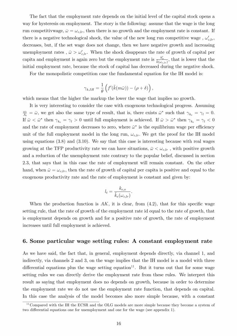
The fact that the employment rate depends on the initial level of the capital stock opens a

way for hysteresis on employment. The story is the following: assume that the wage is the long

run competitivwage, �! = !c;lr, then there is no growth and the employment rate is constant. If

there is a negative technological shock, the value of the new long run competitive wage , !0c;lr,

decreases, but, if the set wage does not change, then we have negative growth and increasing

unemployment rates , �! > !0c;lr. When the shock disappears the rate of growth of capital per

capita and employment is again zero but the employment rate is k0o~k(!c;lr)

, that is lower that the

initial employment rate, because the stock of capital has decreased during the negative shock.

For the monopolistic competition case the fundamental equation for the IH model is:

k;IH =1

�

�f 0(~k(m�!))� (�+ �)

�,

which means that the higher the markup the lower the wage that implies no growth.

It is very interesting to consider the case with exogenous technological progress. Assuming!tAt= �!, we get also the same type of result, that is, there exists �!� such that ke = l = 0.

If �! < �!� then ke = l > 0 until full employment is achieved. If �! > �!� then ke = l < 0

and the rate of employment decreases to zero, where �!� is the equilibrium wage per e¢ ciency

unit of the full employment model in the long run, !c;lr: We get the proof for the IH model

using equations (3.8) and (3.10). We say that this case is interesting because with real wages

growing at the TFP productivity rate we can have situations, �! < !c;lr , with positive growth

and a reduction of the unemployment rate contrary to the popular belief, discussed in section

2.3, that says that in this case the rate of employment will remain constant. On the other

hand, when �! = !c;lr, then the rate of growth of capital per capita is positive and equal to the

exogenous productivity rate and the rate of employment is constant and given by:

lt =ke;o

~ke(!c;lr).

When the production function is AK, it is clear, from (4.2), that for this speci�c wage

setting rule, that the rate of growth of the employment rate id equal to the rate of growth, that

is employment depends on growth and for a positive rate of growth, the rate of employment

increases until full employment is achieved.

6. Some particular wage setting rules: A constant employment rate

As we have said, the fact that, in general, employment depends directly, via channel 1, and

indirectly, via channels 2 and 3, on the wage implies that the IH model is a model with three

di¤erential equations plus the wage setting equation11. But it turns out that for some wage

setting rules we can directly derive the employment rate from these rules. We interpret this

result as saying that employment does no depends on growth, because in order to determine

the employment rate we do not use the employment rate function, that depends on capital.

In this case the analysis of the model becomes also more simple because, with a constant

11Compared with the IH the ECSR and the OLG models are more simple because they become a system oftwo di¤erential equations one for unemployment and one for the wage (see appendix 1).

16

unemployment rate, we close the model using only the fundamental equations. To obtain

these cases we need to have, �rst, that the wage set is a constant markup, m! > 1, over an

alternative reservation wage, %t, that is !t = m!%t. This is a typical result for static wage

setting models but when there is growth to obtain this result is more complicated because

the wage set a¤ects the accumulation of capital via channels 2 and 3. In order to avoid this

problem in models with unions it is assumed that, for some reason, "the union fails to internalize

the dynamic consequences of today�s wage setting on capital accumulation (Ma¤ezzoli (2001),

p.869)"and, then, on future employment. This may happen if the union does not care about

future employment or it is su¢ ciently small so that, changing wages, it does not a¤ect the

accumulation of capital via channels 2 and 3. Van der Ploeg (1987) and Sorolla (1995) present

models where these dynamic consequences are taken into account.

In models with unions, because the mark up depends on the elasticity of labor demand in

order to have a constant mark up we need a constant elasticity of the labor demand, that is a

Cobb-Douglas production function when the product market is competitive With monopolistic

competition and linear production function, Yi = Li, the elasticity of the labor demand depends

only on the markup, m12. In the e¢ ciency wage models where in order to have a a constant

mark up we need an special e¤ort function13 but not a Cobb-Douglas production function.14

The second step consists in specifying a convenient reservation wage, with the following

cases:

Case 1 (Raurich and Sorolla (2003b), Sorolla (2000)). If the alternative wage is the unem-

ployment bene�t, bt,15 %t = bt, that is:

!t = m!bt,

and the unemployment bene�t is �nanced by taxes on employed workers, where � is the tax

rate, i.e.

bt =�!tLtNt � Lt

,

combining these we have:

!t = m!�!tLtNt � Lt

,

and, in terms of the employment rate:

1 = m!� lt1� lt

,

so that the employment rate is:

12See Sorensen and Whitta-Jacobsen (2005), section 3.13The e¤ort function needs to be e(!) = (!�rr )� if ! > r where 0 < � < 1.14Raurich and Sorolla (2003a) and Kaas and von Thadden (2003) are models with a non constant labor

demand elasticity.15This assumption makes sense when wages are set at a national level, that is, for the overall economy.

17

lt =1

(1 + �m!)= l� < 1,

if � > 0. Hence, the employment rate is constant over time and does not depend on growth.

In this case the dynamics of models with unemployment are of the same type as those of

the full employment models. Consider for example, the IH model, when growth depends on

employment, that is, when the production function is not an AK function. From equations

(3.1) and (3.2) we get:

_ctct=1

�(FK(kt; l

�)� (�+ �)) , (6.1)

_kt = f(kt; l�)� ct � (n+ �)kt. (6.2)

and in the full employment model the equations are:

_ctct=1

�(FK(kt; 1)� (�+ �)) ,

_kt = f(kt; 1)� ct � (n+ �)kt.

Because l� < 1, it is clear that the rate of growth of capital per capita is lower for a given

level of c and k in a model with unemployment. Then economies with a constant rate of

unemployment grow less than economies with full employment. It is also clear, from (6.1)

and (6.2), that consumption and capital per capita converge to a steady state with zero rate

of growth of capital per capita and consumption per capita. In this case, with a neoclassical

production function and this particular wage setting rule, there is no relationship between

growth and unemployment in the long run: the constant rate of unemployment is given by l�

and the rate of growth of income per capita is zero, or x, if there is technological progress.

The version of the Ramsey model with non competitive labor and product markets and this

particular wage setting rule implies, then, that there is no relationship between growth and

unemployment in the long run. As shown in the appendix the same result holds for the two

other ways of generating savings. It is also easy to see, drawing the phase diagram, that a

decrease in l� decreases the long run level of consumption, capital and income per capita, that

is, there is a positive relationship between income, capital and consumption per capita and

employment in the long run. In other words, all other parameters equal, economies with full

employment have a higher level of income per capita in the long run that economies with

unemployment.

Using equation (3.5), the rate of growth of wages is given by:

! =1

d~kd!t

!t~k

k:

so that it also converges to zero. When there is productivity growth, using equation (3.10), the

rate of growth of wages is given by:

18

! =1

d~k

d�!tAt

� !tAt~k

k + x:

that converges to x.

When employment does not depend on growth any shock that a¤ects growth is translated

immediately to wages leaving the unemployment rate una¤ected, that is, there is no (short or

long run) e¤ect of productivity on the rate of unemployment. Blanchard and Katz (1997) say

that any model with unemployment should satisfy the condition that there is no long run e¤ect

of the level of productivity on unemployment (p.56).

If the production function is an AK production function, with this wage rule it turns out

that growth does not depend on employment and employment does not depend on growth

and we have constant growth and employment rates. For the IH model we have obtained

lt = l� = 1(1+�m!)

and k = k = �IHAK = 1�(�A� (�+ �)). In this case, then, there is no

relationship between growth and unemployment because the parameters that a¤ect l� and �

are di¤erent. This does not mean that in general with an AK production and a wage setting

rule that implies a constant employment rate, there is no relationship between growth and

unemployment because it can be the case that an exogenous parameter a¤ects both rates. We

present below an example where this happens.

Case 2: The other alternative assumption is that the alternative wage is the average labor

income16, that is, rt = lt(1� �)!t+(1� lt)bt17. Assuming again that the unemployment bene�tis �nanced by taxes on employed workers:

bt =�!tLtNt � Lt

=�!tlt1� lt

combining these we get:

!t = m!!tlt,

so that the employment rate is:

lt =1

m!

= l� < 1.

Alternatively, one can assume that the unemployment bene�t is proportional to the wage

that is bt = '!t18. In this case we have:

!t = m! (lt(1� �)!t + (1� lt)'!t) ,

and the employment rate is:

lt =1� 'm!

(1� �)m! � 'm!

= l�.

16This assumption makes sense if wages are set in a descentralized way.17In a similar way Romer (2006) p.454 assumes: rt = (1� but)!t18For example Pissarides (1990) or Raurich, Sala and Sorolla (2006).

19

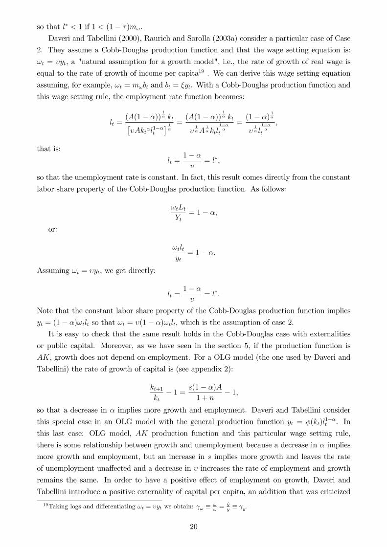
so that l� < 1 if 1 < (1� �)m!.

Daveri and Tabellini (2000), Raurich and Sorolla (2003a) consider a particular case of Case

2. They assume a Cobb-Douglas production function and that the wage setting equation is:

!t = �yt, a "natural assumption for a growth model", i.e., the rate of growth of real wage is

equal to the rate of growth of income per capita19 . We can derive this wage setting equation

assuming, for example, !t = m!bt and bt = �yt. With a Cobb-Douglas production function and

this wage setting rule, the employment rate function becomes:

lt =(A(1� �))

1� kt�

�Akt�l1��t

� 1�

=(A(1� �))

1� kt

�1�A

1�ktl

1���

t

=(1� �) 1�

�1� l

1���

t

,

that is:

lt =1� ��

= l�,

so that the unemployment rate is constant. In fact, this result comes directly from the constant

labor share property of the Cobb-Douglas production function. As follows:

!tLtYt

= 1� �,

or:

!tltyt

= 1� �.

Assuming !t = �yt, we get directly:

lt =1� ��

= l�.

Note that the constant labor share property of the Cobb-Douglas production function implies

yt = (1� �)!tlt so that !t = �(1� �)!tlt, which is the assumption of case 2.It is easy to check that the same result holds in the Cobb-Douglas case with externalities

or public capital. Moreover, as we have seen in the section 5, if the production function is

AK, growth does not depend on employment. For a OLG model (the one used by Daveri and

Tabellini) the rate of growth of capital is (see appendix 2):

kt+1kt

� 1 = s(1� �)A1 + n

� 1,

so that a decrease in � implies more growth and employment. Daveri and Tabellini consider

this special case in an OLG model with the general production function yt = �(kt)l1��t . In

this last case: OLG model, AK production function and this particular wage setting rule,

there is some relationship between growth and unemployment because a decrease in � implies

more growth and employment, but an increase in s implies more growth and leaves the rate

of unemployment una¤ected and a decrease in � increases the rate of employment and growth

remains the same. In order to have a positive e¤ect of employment on growth, Daveri and

Tabellini introduce a positive externality of capital per capita, an addition that was criticized

19Taking logs and di¤erentiating !t = �yt we obtain: ! � _!! =

_yy � y.

20

by Sala-i-Martin (2000), section 2.8.

7. Wage setting rules with inertia

If we add inertia (persistence) to the wage setting rules of Section 6, so that wage setting

depends also on past values of wages and employment rates then the IH model yields a system

of four di¤erential equations with dynamics for both employment rates and wages. In section

6 the unemployment rate was constant and in section 5 the wage was constant so that one of

the four di¤erential equations was eliminated.

There are several ways of introducing inertia, the usual are the following:

Case 1: Wage inertia (Raurich and Sorolla (2003b), Sorolla (2000)). In this case the set

wage is, as usual, a mark-up over the reservation wage, !t = m!%t, but the reservation wage is

a weighted average of the current unemployment bene�t and past wages. In the OLG model

where workers work for one period past wages are the wages of parents.

Blanchard and Katz (1997) justify wage inertia on the reservation wage saying that "models

based on fairness suggest that the reservation wage may depend on factors such as the level and

the rate of growth of wages in the past, if workers have come to consider such wage increases

as fair. Perhaps a better word than "reservation" wage in that context is an "aspiration" wage

(p.54)". Wage inertia is derived in an e¢ cient wage model where workers�disutility depends

on the comparison between current and past wages (see Collard and de la Croix. (2000), de la

Croix et al. (2000) and Danthine and Kursmann (2004)). Empirical evidence shows that there

is wage persistence in the wage setting process (see Blanchard and Katz (1997) and (1999) and

Hogan (2004)).

We introduce wage persistence in the discrete time version considering: %t = �!t�1+(1��)bt,where 0 5 � 5 1. Combining with the wage setting equation we get:

!t = m!(�!t�1 + (1� �)bt).

In order to obtain the continous time version we substract !t�1 and, making !t�1 = !t, we

obtain:

_!t = (�m! � 1)!t + (1� �)m!bt

If the unemployment bene�t is �nanced by taxes, i.e.

bt =�!tLtNt � Lt

=�!tlt1� lt

,

we get for the continuos time version:

_!t = (�m! � 1)!t + (1� �)m!�!tlt1� lt

. (7.1)

Assuming that the model converges20 to an steady state where ! = l = 0, from equation

20With this wage setting rule Sorolla (2000) studies the conditions for convergence in an OLG model withconstant saving rate, neoclassical production function and exogenous technological progress. Raurich and Sorolla

21

(7.1) we get:

l� =1� �m!

1� �m! + (1� �)�m!

.

Assuming 0 5 � then 0 < l� < 1. Moreover, if ! = l = 0 then, by (3.5), k = 0, which isonly possible with a neoclassical production function. This means that if the model converges

to an steady state it turns out that growth stops. This should not be a surprise because this is

Case 1 of section 6, where in the long run growth stops, plus wage inertia. The novelty here is

that the long run employment rate depends on the degree of wage inertia, �, having @l�

@�< 0,

that is, a higher degree of wage inertia reduces the long run employment rate. The introduction

of wage inertia means that a productivity shock a¤ects the employment rate in the short run

but not in the long run. With wage inertia, then, there is also no relationship between growth

and unemployment in the long run without technological progress. If the production function

is AK, Raurich and Sorolla (2003b) show that, with wage inertia, growth a¤ects employment

in the long run.

With exogenous technological progress, equation (7.1) becomes:

_!tAt= (�m! � 1)

!tAt+ (1� �)m!

� !tAtlt

1� lt,

or: �_!tAt

�= (�m! � 1)

!tAt+ (1� �)m!

� !tAtlt

1� lt� x!t

At, (7.2)

and hence in an steady state where !A= l = 0, using (7.2) we obtain:

l� =1� �m! + x

1� �m! + x+ (1� �)�m!

.

Here the novelty is that the rate of employment in the long run depends on the degree of wage

inertia, � and the productivity rate x, having @l�

@�< 0 and @l�

@x> 0, that is, a higher degree of

wage inertia reduces the long run employment rate. Because in an steady state !A= l = 0,

with a neoclassical production function, then ke = 0. So that the rate of growth of wages is

equal to the rate of growth of capital per capita and they are equal to the productivity growth

rate. This means that with wage inertia and technological progress there is some relationship

between growth and unemployment in the long run in the sense that an increase in x implies

more growth and more employment in the long run21. It follows that in the version of the

Ramsey model with non competitive labor and product markets and wage inertia there is some

relationship between growth an unemployment in the long run. The same result holds for the

two other ways of generating savings. This is easy to see looking at the fundamental equations

(2003b) study the convergence conditions when the production function is an AK production function due toproductive government expenditures (and without exogenous technological progress).21The wage equation obtained in the continuos case, assuming !t�1 = !t in the discrete time case, produces

the weird result that when � = 0 then l� = 1+x1+x+�m!

, whereas for this case in the previous section we haveobtained l� = 1

1+�m!. This is because the "forced" version of wage inertia in continuos time. For the discrete

time version everything works, but we mantain here the continuos version in order to have the model in thesame type of time.

22

derived in appendix.

Case 2: Labor income inertia (Raurich, Sala and Sorolla (2006)). As in the previous case

the set wage is a mark-up over the reservation wage, !t = m!%t, but the reservation wage is

a weighted average of past average labor income, that is, there is labor income inertia. In the

discrete time version we have: %t = �(lt�1(1��)!t�1+(1�lt�1)bt�1)+�(1��)(lt�2(1��)!t�2+(1� lt�2)bt�2)+�(1��)2(lt�3(1� �)!t�3+(1� lt�3)bt�3)+ ::: where 0 < � 5 122. We transformlast equation into a di¤erence equation of the form:

rt = � [lt�1(1� �)!t�1 + (1� lt�1)bt�1] + (1� �)rt�1.

And, hence, the continuos time version is:

_rt = �([lt(1� �)!t + (1� lt�1)bt]� rt).

If the unemployment bene�t is �nanced by taxes23, i.e.:

bt =�!tLtNt � Lt

=�!tlt1� lt

,

we get for the continuos time version:

_rt = �(lt!t � rt).

From !t = m!rt we get _!t = _rt and also rt = !tm!, expressions that, when substituted to in the

last equation, give:

_!t = �(lt!t �!tm!

). (7.3)

Hence, in an steady state:

l� =1

m!

< 1.

We have the same result in the long run that the we obtained in Case 2 of the constant

employment rate section. Thus there is no relationship between growth and unemployment in

the long run when the production function is neoclassical.

With exogenous technological progress (7.3) becomes:

_!tAt= �(lt

!tAt�

!tAt

m!

),

or: �_!tAt

�= �(lt

!tAt�

!tAt

m!

)� x!tAt,

and hence, in the steady state:

22The case � = 0 makes no sense. If � = 1 then rt = lt�1(1� �)!t�1 + (1� lt�1)bt�1. A similar result holdsif we link the wage with past income per capita, that is, !t = �yt�1 + �(1 � �)yt�2 + �(1 � �)2yt�3 + ::: andhave a Cobb-Douglas production function.23Or bt = �!t as in Raurich Sala and Sorolla (2006).

23

l� =1

m!

+x

�.

Here the novelty is that the rate of employment in the long run depends on the degree of past

labor income inertia, � and the productivity growth rate x, that is, in the version of the Ramsey

model with non competitive labor and product markets and labor income inertia there is some

relationship between growth and unemployment in the long run. As shown in the appendix the

same result holds for the two other ways of generating savings.

8. Conclusions

In this paper we have derived the set up that shows clearly that, in growth models with

disequilibrium unemployment, in general the growth rate of capital depends on the employment

rate (growth depends on employment) and the employment rate depends on the stock of capital

(employment depends on growth) and how both variables depend on the real wage and, with

monopolistic competition in the output market, on markups. The �rst relationship gives rise to

the fundamental equations of a growth model with unemployment that we derive explicitly for

the standard growth models: exogenous constant saving rate, in�nite horizon and overlapping

generations, and we compare them with the ones obtained in the models with full employment.

Once we have made explicit the fundamental equations, in order to close the models, we

need to specify a wage equation. Then, it turns out that the relationship between growth and

unemployment will depend on the speci�c wage setting rule and on the form of the production

function.

We show that if the production function is AK growth does not depend on employment

and, hence, not on wages.

When the production function is neoclassical, we analyze the behavior of the models with

the standard wage setting rules. When a constant real wage is set, if this wage is lower that

the long competitive real wage then there is always a constant positive rate of growth of capital

and full employment in the long run, that is, there is a relationship between them in the long

run. If this wage is the long competitive real wage then there is no growth of capital per capita

and employment remains constant and depends on the initial level of the stock capital, result

that opens the door for hysteresis on unemployment.

If the rule implies a constant employment rate (employment does not depend on growth)

then economies with a constant rate of unemployment grow less than economies with full

employment and the long run rate of growth of income per capita is equal to the productivity

rate, that is, there is no relationship between growth and unemployment in the long run for the

three standard ways of generating saving, in particular for the Ramsey model (the canonical

model of growth) with unemployment.

If inertia, which depends on past wages or past labor incomes, is present in the wage setting

process, we show that, a smaller degree of inertia or a faster productivity growth implies a

smaller run long rate of unemployment. Thus, since the long run rate of income per capita is

equal to the productivity rate, there is some relationship between growth and unemployment

24

in the long run for the three standard ways of generating saving, in particular, again, for the

Ramsey model with unemployment.

9. References

Aghion, P. and Howitt, P. (1994). �Growth and Unemployment�, Review of Economic Studies

61: 477-94.

Aghion, P. and Howitt, P. (1998). Endogenous Growth Theory, The MIT Press.

Anderson, S. and Devereux, M. (1988). "Trade Unions and the Choice of Capital Stock",

Scandinavian Journal of Economics 90(1): 27-44.

Aricó, F. (2003). �Growth and Unemployment: Towards a Theoretical Integration �, Jour-

nal of Economic Surveys 17: 419-455.

Barro, R.G. and Sala-i-Martin, X. (2003). "Economic Growth", 2nd edition. The MIT

Press.

Bean, C. and Pissarides, C.A. (1993). �Unemployment, Consumption and Growth�, Euro-

pean Economic Review 37: 837-54.

Benassy, J.P. (1997). "Imperfect Competition, Capital Shortages and Unemployment Per-

sistence", Scandinavian Journal of Economics 99(1): 15-27.

Bentolila, S and Saint-Paul, G. (2003). �Explaining Movements in the Labour Share�, Con-

tributions to Macroeconomics 3 (1): Article 9. http://www.bepress.com/bejm/contributions/vol3/iss1/art9.

Blanchard, O. and Katz, L.F. (1997). �What We Know and Do Not Know About the

Natural Rate of Unemployment�, Thw Journal of Economic Perspectives 11(1): 51-72.

Blanchard, O. and Katz, L.F. (1999). �Wage Dynamics: Reconciling Theory and Evidence�,

NBER Working Paper 6924.

Daveri, F. and Mafezzoli, M. (2000). "A numerical approach to �scal policy, unemployment

and growth in Europe", unpublished manuscript.

Collard, F. and de la Croix, D. (2000). �Gift Exchange and the Business Cycle: The Fair

Wage Strikes Back�, Review of Economic Dynamics 3: 166-193.

De la Croix, D., Palm, F.C. and Urbain, J. (2000). �Labor Market Dynamics when E¤ort

Depends on Wage Growth Comparisons�, Empirical Economics 25: 393-419.

Danthine J.-P, and Kurmann, A. (2004);"Fair wages in a New Keynesian model of the

business cycle", Review of Economic Dynamics 7: 107-142.

Daveri, F. and Ma¤ezzoli, M. (2000). "A numerical approach to �scal policy, unemployment

and growth in Europe", Unpublished manuscript.

Daveri, F. and Tabellini, G. (2000). "Unemployment and Taxes", Economic Policy, 5:

49-104.

Domenech, R. and García, J.R. (2008). "Unemployment, taxation and public expenditure

in OECD economies", European Journal of Political Economy 24: 202-217.

Eriksson, C. (1997). �Is There a Trade-O¤ between Employment and Growth?�Oxford

Economic Papers 49: 77-88.

Galí, J. (1995). "Non-Walrasian Unemployment Fluctuations", NBERWorking Paper 5922.

25

Galí, J. (1996a). "Multiple equilibria in a growth model with monopolistic competition",

Economic Theory 8: 251-266.

Galí, J. (1996b). "Unemployment in dynamic general equlibrium economies", European

Economic Review 40: 839-845.

Hogan V. (2004). "Wage aspirations and unemployment persitence", Journal of Monetary

Economics 51: 1623-1643.

Kaas, L. and von Thadden, L. (2003). "Unemployment, Factor Substitution and Capital

Formation", German Economic Review 4 (4): 475-495.

Mafezzoli, M. (2001). "Non-Walrasian Labor Markets and Real Business Cycles", Review

of Economic Dynamics 4: 860-892.

McDonald, I. A. and Solow R.M. (1981). "Wage Bargaining and Unemployment", American

Economic Review 71: 896-908.

Mortensen, D.T. and Pissarides, C.A. (1998). "Technical Progress, Job Creation and Job

Destruction", Review of Economic Dynamics, 1: 733-753.

Mortensen, D.T.(2005). "Growth, Unemployment and Labor Market Policy", Journal of

the European Economic Association, 3(2-3): 236-258.

Pissarides, C.A. (1990). "Equilibrium Unemployment Theory", Basil Blackwell..

Raurich X., Sala, H. and Sorolla, V. (2006). �Unemployment, Growth and Fiscal Policy,

New Insights on the Hysteresis Hypothesis�, Macroeconomic Dynamics, 10: 285-316.

Raurich X. and Sorolla, V. (2003a). �Growth, Unemployment and Public Capital�, Spanish

Economic Review, 5: 49-61.

Raurich X. and Sorolla, V. (2003b). �Unemployment and Wage Formation in a Growth

Model with Public Capital�, Unpublished manuscript.

Romer, D. (2006). "Advanced Macroeconomics", Third edition. McGraw-Hill.

Sala-i-Martin, X. (2000). "Apuntes de Crecimiento Económico", 2a edición. Antoni Bosch

editor.

Solow R.M. (1979). "Another Possible Source of Wage Stickiness", Journal of Macroeco-

nomics 1: 79-82.

Sorensen, P.B. andWithha-Jacobsen, H.J. (2005). "Introducing Advanced Macroeconomics:

Growth ans Business Cycles", McGraw Hill.

Sorolla, V. (1995). �Sindicatos, Gobierno, Inversión y nivel de empleo en el futuro�, Revista

Española de Economía 2a epoca, 12: 141-162.

Sorolla, V. (2000). �Growth, Unemployment and the Wage Setting Process�, Unpublished

manuscript.

Van der Ploeg, F. (1987). "Trade Unions, Investment and Unemployment: A Non-Cooperative

Approach", European Economic Review 31: 1465-1492.

10. Appendix 1

10.1. The ECSR model

26

We consider the case of a constant saving rate, s, exogenous and independent of the interest

rate which means that channel 2 is inactive. Consider the following equation for the supply of

capital Kst24 in continuos time25:

_Kst = rtKt + !tLt � Ct

where Ct is total consumption. In per capita terms we have:

_kst = rtkt + !tlt � ct � nkt.

In the last equation channel three becomes transparent, a change in the wage a¤ects aggregate

income, rtkt + !tlt, changing ! and, indirectly, l and r, that is, the wage a¤ects growth.

Equilibrium in capital market, kst = kdt = kt, and the zero pro�ts condition, (2.5), imply:

_kt = F (kt; lt)� ct � (n+ �)kt.

Assuming that savings are a constant proportion of output, that is, there is a constant rate of

saving s, we have ct = (1� s)F (kt; lt), which implies:

_kt = sF (kt; lt)� (n+ �)kt. (10.1)

Note that the di¤erence between this equation and the fundamental equation of the ex-

ogenous constant saving rate model with a competitive labor market with full employment:_kt = sf(kt) � (n + �)kt is in the production function26 The production function in (10.1) de-pends on the employment rate, because there is no full employment. Also note that, in this

model, employment a¤ects growth because a higher level of lt increases the growth of capital

per capita.

Dividing by kt we get the equation in terms of the capital per capita growth rate, k �_ktkt27:

k =sF (kt; lt)

kt� (n+ �) = sF (1; lt

kt)� (n+ �) = s ~f( lt

kt)� (n+ �) = s ~f( 1

kt)� (n+ �).

Now substituting in the last equation the capital labor ratio we get:

k;ECSR �_ktkt= s ~f(

1~k(!t)

)� (n+ �). (10.2)

We call to this equation the fundamental equation of a model with an exogenous constant

savings rate and wage setting. Note that, in equilibrium, channel three is transformed into the

e¤ect of the wage on output per unit of capital, via the capital labor ratio. If the wage increases,

then output per unit of capital decreases, due to the increase in the capital labor ratio, and,

24Alternativelly, we can use the notation Kst = Bt, where the Bt are �nancial assets or bonds.

25Because there is unemployment it may be the case that the unemployed people get some unemploymentbene�t, when they do, we assume that this unemployment bene�t is �nanced by taxes on capital and wageincome. If the government budget constraint is balanced then we get this equation.26In the full employment equation we also have kt = kt because Nt = Lt.27From now on we will de�ne the rate of growth of a variable by the letter .

27

then, the rate of growth of capital decreases. We can say that if the production function has

the usual properties, without ambiguities, via channel three, an increase in the wage implies a

decrease in aggregate income per unit of capital and a decrease in the rate of growth of capital

per capita and, then, less capital per capita and a lower employment rate in the future.

Note that in principle, we can not solve the fundamental equation, this means that we can

not compute kt and hence to obtain the employment rate lt from this equation, but we can

compute the evolution of the employment rate using (3.5).

Finally substituting (10.2) into (3.5) we get:

l;ECSR = s~f(

1~k(!t)

)� (n+ �)� d~k

d!t

!t~k

_!t!t, (10.3)

which is a di¤erential equation in terms of the employment rate and the wage. Once we have

the fundamental equation, the closing of the model depends on how the wage is set.

For the monopolistic competition case it also turns out (see Galí (1996) section three) that

the equation for the evolution of the composite stock of capital is also:

_kt = F (kt; lt)� ct � (n+ �)kt.

Assuming a constant savings rate and substituting in the capital labor ratio we get the funda-

mental equation:

k;ECSRMC �_ktkt= s ~f(

1~k(m!t)

)� (n+ �), (10.4)

where an increase in the mark up also decreases the rate of growth of capital per capita so that

there is less capital per capita and a lower employment rate in the future.

It is also useful to derive the fundamental equation with technical progress in continuos

time. Rewriting the supply of capital in terms of the supply of capital per e¢ ciency person

and assuming equilibrium we get :

_ke;t = sF (ke;t; lt)� (n+ � + x)ke;t,

or, in terms of the growth rate of capital per e¢ ciency person, ke :

ke =sF (ke;t; lt)

ke;t�(n+�+x) = sF (1; lt

ke;t)�(n+�+x) = s ~f( lt

ke;t)�(n+�+x) = s ~f( 1

ke;t)�(n+�+x).

Substituting into the last equation the capital e¢ ciency labor ratio function we get:

ke;ECSSRTP �_ke;tke;t

= s ~f(1

~k( !tAt))� (n+ � + x). (10.5)

Note that depending on the value of !tAtwe can have a positive rate of growth of capital per

e¢ ciency person, this case is discussed for the IH model in section 6.

28

10.2. OLG

We consider an OLG model where the agents live two periods and have the utility function:

Ut =C1��1t

1� � +1

1 + %

C1��2t+1

1� � ,

where � > 0. When � = 1 utility is logarithmic. If � 6= 1 it turns out that channel two is activebecause the saving rate depends on the interest rate. The savings rate function ~s(rt+1) is given

by (Romer (2006), section 2.9) :

st = ~s(rt+1) =(1 + rt+1)

1���

(1 + %)1� + (1 + rt+1)

1���

=1

(1+%)1�

(1+rt+1)1���

+ 1.

If � < 1 then ~s0 > 0 and if � > 1 then ~s0 < 0. Using the interest rate function (2.9) we get:

st = s(!t+1) = ~s(~r(!t+1)) =1

(1+%)1�

(1+f 0(~k(!t+1))��)1���

+ 1

with s0 < 0 if � < 1 and s0 > 0 if � > 1:

The accumulation of capital is given by the equation (see also Romer (2006) ):

Kt+1 = s(!t+1)!tLt,

that is, in per capita terms:

kt+1 =1

1 + ns(!t+1)!tlt,

where it is also evident that channel three is active because a change in the wage modi�es labor

income. Using the employment rate function (2.11), we get:

kt+1kt

=1

1 + n

s(!t+1)!t~k(!t)

.

Then the rate of growth of capital per capita, in discrete terms, the fundamental equation,

is given by:

k;OLG =kt+1kt

� 1 = 1

1 + n

s(!t+1)!t~k(!t)

� 1 (10.6)

.

Using the employment rate function (2.11), the employment rate is given by the di¤erence

equation:

lt+1 =kt+1~k(!t+1)

=1

1 + n

s(!t+1)!tlt~k(!t+1)

, (10.7)

and the rate of growth of the employment rate is:

29

l;OLG =lt+1lt� 1 = kt+1

kt

~k(!t)~k(!t+1)

� 1 = 1

1 + n

s(!t+1)!t~k(!t+1)

� 1, (10.8)

a di¤erence equation in terms of employment and the wage.

In the monopolistic competition case the equations become:

k;OLGMC =kt+1kt

� 1 = 1

1 + n

s(m!t+1)!t~k(m!t)

� 1, (10.9)

and

l;OLGMC =lt+1lt� 1 = kt+1

kt

~k(m!t)~k(m!t+1)

� 1 = 1

1 + n

s(m!t+1)!t~k(m!t+1)

� 1. (10.10)

With exogenous technological progress (now ke;t = Kt

AtNt) they are:

ke;OLGETP =ke;t+1ke;t

� 1 = 1

(1 + n)(1 + x)

s( !t+1At+1

) !tAt

~k( !tAt)

� 1 (10.11)

and

l;OLGETP =lt+1lt� 1 = ke;t+1

ke;t

~k( !tAt)

~k( !t+1At+1

)� 1 = 1

(1 + n)(1 + x)

s( !t+1At+1

) !tAt

~k( !t+1At+1

)� 1. (10.12)

With a logarithmic utility function it turns out that the savings rate does not depend on

the interest rate28, that is channel two is inactive and, in this case, we only have to substitute

s for the savings function in the previous fundamental equations (10.6), (10.9) and (10.11).

11. Appendix 2 The AK model

In this case the fundamental equation of a model with an exogenous constant saving rate (10.2)

becomes:

k;ECSSR = sA

�1

kt

�1���K1��t � (n+ �) = sA

�1

kt

�1��k1��t � (n+ �) = sA� (n+ �) = �ECSRAK ,

and, then, channel 3 is inactive29, and growth does not depend on employment. This means

that the rate of growth of capital and income per capita does not depend on the wage setting.

From (4.1) we get:

l = k � ! = �ECSRAK � !:28We get s = 1

2+� .29Channel 2 is also inactive because of the assumption of a constant savings rate independent of the interest

rate.

30

That is, the growth rate of the employment rate depends on capital growth and wage growth,

and the wage dynamics a¤ect only the dynamics of employment. For the same reason if the

output market is not competitive a change in the markup does not a¤ect growth and the labor

demand is given by:

lt =A(1� �)ktm!t

. (11.1)

Finally, we consider the OLG model with a constant saving rate s. In this case, it is easy

to check that:

!tLt = (1� �)AKt

and, because,

Kt+1 = s!tLt,

we have:Kt+1

Kt

= s(1� �)A:

The fundamental equation is given by:

kt+1kt

� 1 = s(1� �)A1 + n

� 1 = �OLGAK ,

which shows that growth does no depend on employment30. In this case the rate of growth of

the employment rate is given by:

lt+1lt� 1 =

�s(1� �)A1 + n

!t!t+1

�� 1.

Daveri and Tabellini (2000) present an OLG model where they consider as special case the

production function Yt = AKt�L1��t

�Kt1�� where the externality, instead of being �Kt = kt, is

capital per person �Kt = kt:With this production function it turns out that:

!tLt = (1� �)AKtlt

so that:

Kt+1

Kt

= s(1� �)Alt:

Thus growth depends on employment. This particular externality is criticized in Sala-i-

Martín (2000), section 2.8.

30This is the set up of Raurich and Sorolla (2003b), where for a speci�c real wage dynamics, the e¤ect oftaxes on growth and long run employment is studied.

31