WP-2007-016

A General Equilibrium Open Economy Model for Emerging Markets:

Monetary Policy with a Dualistic Labor Market

Ashima Goyal

Indira Gandhi Institute of Development Research, Mumbai October 2007

2

A General Equilibrium Open Economy Model for Emerging Markets:

Monetary Policy with a Dualistic Labor Market 1

Ashima Goyal

Indira Gandhi Institute of Development Research (IGIDR) General Arun Kumar Vaidya Marg

Goregaon (E), Mumbai- 400065, INDIA Email: ashima@igidr.ac.in

Abstract

An optimizing model of a small open emerging market economy (SOEME) with dualistic labour markets and two types of consumers, delivers a tractable model for monetary policy. Differences between the SOEME and the SOE are derived. Parameters depend on features of the labour market and on consumption inequality, and affect the natural interest rate, terms of trade and potential output. The supply curve turns out to be flatter and more volatile, with a larger number of shift factors. A simple basic version of the model is simulated in order to compare different policy targets in response to a cost shock. Flexible domestic inflation targeting delivers stability and the lowest volatility. Some weight on output and on interest smoothing allows monetary policy to be less contractionary. Exchange rate flexibility is less but still makes a major contribution to controlling inflation.

Key words: small open emerging market, optimal monetary policy, dualistic labour markets,

terms of trade, potential output JEL Code(s): E52, F41

1 An earlier version of the paper was presented in the IGIDR-Northwestern-RBI conference on “Advances in Open Economy Macroeconomics”, Mumbai. I am grateful for the useful comments received in particular from Craig Burnside, V.V. Chari, Lawrence Christiano, Romar Correa, Pierre-Olivier Gourinchas, Bruce Preston, Pedro Teles, and Linda Tesar. I thank the Fulbright Foundation for financial support and Claremont University for hospitality during the period the basic model was developed, Kaushik Basu, Ajay Gupta, Amarava Roy, Ekta Sehgal, Manish Dureja, Poulomi Maitra, Raghav Mathur, Shaista Kassim, Shobhini Chhabra, Sonal Garg, Sumedh Deorukhkar, and Vandana Chauhan for comments, Paul Soderlind for the Matlab programs used and Tony Calvoli and Ramkishen Rajan for introducing me to them, Suvarna Gurav for introducing me to Matlab and for trouble-shooting programs, and T. S. Ananthi and Jayashree for secretarial assistance.

3

A General Equilibrium Open Economy Model for Emerging Markets:

Monetary Policy with a Dualistic Labor Market

Ashima Goyal

1. Introduction Monetary policy has been analyzed for open economies in dynamic stochastic general equilibrium models with imperfect competition and nominal rigidities 2, and is found to have substantial effects on real variables. Product diversity gives market power to individual producers under monopolistic competition implying output is suboptimally low. This, together with some type of price stickiness, allows monetary policy to have real effects. Further developments have reduced the policy problem to an elegant optimization subject to microfoundation based aggregate demand and supply curves with forward-looking behaviour3. Being derived from basic technology, preferences and market structure, the coefficients of the equations are robust to policy changes, thus meeting the Lucas critique. This paper seeks to systematically analyze differences in the model, and its results for policy, if the small open economy is an emerging market with a large share of less productive labour in the process of being absorbed into the modern sector. One simple version of the final model developed is calibrated and simulated for a typical small open emerging market economy (SOEME). Optimal responses to a cost shock are derived under different types of targeting. In order to focus on the labour market, simplifying assumptions of complete financial markets and perfect capital mobility are maintained. Two types of consumers and labour are distinguished in the SOEME, those above subsistence (R), and those at subsistence (P). While the first are able to smooth consumption using international markets, those at subsistence cannot. Their intertemporal elasticity of consumption, productivity and wages are lower and their labor supply elasticity is higher, compared to the first group4. All these follow from the key difference—high and low productivity. Differential treatment of these two types partially addresses the Stiglitz objection below, while being able to use the power of the modern benchmark models for monetary policy.

“The standard models taught in graduate schools in the U.S. and Europe are of limited relevance for developing countries. … more disturbing is that virtually all of the research uses full employment models, making the results of questionable relevance, e.g. in a country with 25% unemployment (Stiglitz, 2007).”

CES aggregation allows the micro diversity to be collapsed to macro aggregates, as is common in the literature. The resulting aggregate supply curve is flatter for a SOEME compared to a mature small open economy (SOE), but is less stable, with more factors 2 Obstfeld and Rogoff (1995) is a textbook treatment of a large literature on the new open economy macroeconomics to which they made seminal contributions. Prices in their model were determined one period in advance. Later treatments use variants of staggered prices, which allows smooth aggregate price adjustment. 3 See Clarida et. al (1999) for a survey and Clarida et. al (2001) for extension to an open economy. Woodford (2003) is a rigorous textbook treatment of these results. 4 This subsistence-based definition makes the model suitable for analyzing populous emerging markets such as India and China.

4

tending to shift it. The slope reduces as the economy becomes more open, but the reduction is relatively more for SOE. A key difference between the two kinds of economies is that the real exchange rate for the former is depreciated and tends to appreciate as development brings it closer to purchasing power parity (PPP). But there are fluctuations on the way. The stronger income effects on the terms of trade in a SOE imply that substituting these out makes the aggregate supply curve steeper. This is particularly so for an almost closed economy with a large percentage of P. Therefore it may be better to base policy on aggregate supply without substituting out the terms of trade, and use exchange rate policy to counter the shifts. We derive this variant of aggregate supply also. The difference between average world and SOEME per capita income generates a gap variable, which implies a higher potential output and a trade surplus for the SOEME. This may be part of the explanation of large trade surpluses in many rapidly growing Asian SOEMEs. Consumption of subsistence group is a new exogenous variable in the model for the SOEME. This affects the natural rate of interest, potential output, and the equilibrium terms of trade, in general reducing the effect of world output on these variables, compared to the SOE. The interest elasticity of aggregate demand is lower in the SOEME but there are more factors tending to decrease the natural rate of interest, including expected appreciation of the terms of trade. Regarding aggregate model dynamics, an initial simulation for a cost shock shows flexible targeting of domestic price inflation delivers stability and the lowest volatility, with the least monetary contraction. It involves active use of exchange rate policy to lower the price impact of a cost shock, but fluctuations in the exchange rate are lower than under consumer price and strict direct inflation targeting. The structure of the paper is as follows. The model is developed in Section 2, and its differences from the SOE model noted. Household optimization is in Section 2.1, basic identities are developed in 2.1.1, international risk sharing in 2.1.2, the aggregate demand supply equality in 2.1.3, dynamic aggregate demand, with and without endogenizing the terms of trade, is derived in 2.1.4, uncovered interest parity is set out in 2.1.5. Firms’ optimization is set up and aggregate supply derived in Section 2.2. Natural rates are derived and aggregate demand and supply written in terms of these in Section 3. Some modifications in the basic model to further adapt it to conditions in SOEMEs are discussed in Section 4, and policy response to ensure stability in Section 5. The basic model is tested and optimal policy derived through simulations in Section 6, before Section 7 concludes. Some derivations are in the appendix. 2. A Small Open Emerging Market Model Following Gali and Monacelli (2005) (GM), we assume a continuum of small open economies on the unit interval, but divided into two types—emerging and mature markets5. Since each country is of measure zero, it takes world prices as given. An emerging market has two types of consumers, those above and those below subsistence. The product market structure, technology and preferences of R type consumers are the same across all economies. Productivity shocks differ since emerging markets are in transition stages of applying the new 5 Our model is based on the small open economy models by Svensson (2000), and in particular Gali and Monacelli (2005) (henceforth GM). We try to keep as close as possible to the latter’s formulation in order to facilitate systematic comparison of results.

5

technologies becoming available. P type consumers are assumed to be at a fixed subsistence wage, financed in part by transfers from R types, and they are willing to supply more labor hours to the modern sector at a wage epsilon above their opportunity cost or wages in the informal sector. Variables corresponding to a representative consumer in a mature economy have a superscript i, averages for the world economy as a whole are denoted by a superscript *, while in order to simplify notation superscripts are dropped for the representative consumer in the SOEME. 2.1 Households A typical SOEME has two representative households above subsistence (R) and at subsistence (P). The intertemporal elasticity of consumption (1/σ), productivity and wages (W) of R are higher, their labour supply elasticity (1/ϕ) is lower compared to the P, and they are able to fully diversify risk in international capital markets. Each type seeks to maximize:

∑∞

=⎟⎠⎞

⎜⎝⎛

0 ,,,t tiNtiCUtoE β i = R, P (1)

Ni, t denotes hours of labour, and β is the discount factor. Aggregate consumption Ct is a composite index of consumption of home (H) and foreign goods (F). Elasticity of substitution between H and F goods is assumed to equal unity. In this case the CES aggregation simplifies to Eq. (2) for consumption and Eq. (3) for the price index. Each of CH, t, CF, t are indices of a continuum of differentiated home and foreign goods respectively with elasticity of substitution between goods of different varieties, ε >1, as is required for equilibrium under monopolistic competition. Simplifications are made to reduce the degree of disaggregation, and focus on disaggregation of consumption between the R and the P households6. The corresponding consumer price index can be derived from cost minimization of consumption bundle as is standard in the literature (Obstfeld and Rogoff, 1996). The share of foreign goods, α, 0< α<1, defines the degree of openness. It is inversely related to the degree of home bias, and is assumed to be the same for R and P, since although P spend more on food, agricultural products are also traded goods.

αα

tFCtHkCtC ,1

,−≡ (2)

Where the constant ( ) αα αα −−

= 111k

Given the constant k, the price index can be written as:

αα

tFPtHPtP ,1

,−= (3)

Since the effective terms of trade, or price of foreign goods in terms of home goods, is

tHtFt PPS ,,= , substituting in (3) gives:

6 The implications of disaggregation by type of goods and source have been well explored in the literature (see GM), and these complications can be added after developing our basic model. An elasticity of substitution will affect the trade balance, and the derived coefficients, but the effects will be similar for a SOE and a SOEME. Elasticities of substitution greater than unity would increase the interest elasticity of aggregate demand and decrease the slope of aggregate supply.

6

αttHt SPP ,= (4)

That is, consumer prices depend on domestic prices and the terms of trade. Consumption of each type of good is a weighted average of consumption by the R and the P households, with η as the share of R. The assumption made that H and F are consumed by R and P in the same proportion implies that Ct is distributed between R and P in the same proportion η, where η is the share of above subsistence households in consumption.

ηααηαα

ηη

ηη

⎟⎠⎞

⎜⎝⎛ −−

⎟⎠⎞

⎜⎝⎛ −=

−=

−=

tFRCtHRCtFPCtHPCktC

tRCtPCtFC

tRCtPCtHC

,,1

,,1

,,1

,,

,1

,,

,1

,,

(5)

A household’s period utility function is given the specific form:

( )i

ti

i

tiii

ii NCNCU

ϕσ

ϕσ

+−

−≡

+−

11,

1,

1, i = R, P (6)

Where Ni, t is the labour supplied by each type. Utility is maximized subject to a sequence of period budget constraints:

tititititittttit TNWDDQECP ,,,,1,1,, ++≤+ ++ (7) Where Wi, t is the nominal wage paid to each type, Qt, t+1 is the stochastic discount factor corresponding to the random payoff Dt+1 of the portfolio purchased at t; Rt is the gross nominal yield on a one period discount bond, so that 1,

1+

− = tttt QER is the price of the discounted bond; Ti, t is lump sum taxes or transfers. Taxes from R finance transfers to P; payoffs D are taken as zero for the latter. The government intermediates these transfers and runs a balanced budget so that η TR, t = - (1-η) TP, t where a negative tax is a transfer. The subsidy is calculated to give P a subsistence wage if they work eight hours daily, but they are free to increase their wages by working longer hours. Our assumptions allow us to define the aggregate intertemporal elasticity of substitution, 1/σ, and the inverse of the labour supply elasticity7, ϕ, as weighted sums with population shares of R and P as weights,

( )

( ) PR

PR

ϕηηϕϕ

ση

ση

σ

−+=

−+=

1

1111

(8)

Since P lack the ability to smooth consumption their intertemporal elasticity of consumption approaches zero, so the averaging is better done with elasticities, rather than inverse

7 This is also the elasticity of price with respect to output as will be clear from the aggregate supply curve derived as Eq. (65) below. The labour supply elasticity of P can be expected to be high, and their intertemporal elasticity of consumption low. We normalize the latter at zero. Average ϕ is taken as 0.25 in the simulations, implying a labour supply elasticity of 4.

7

elasticities. The standard first order conditions for optimal allocation of consumption across home and foreign goods yield the demand functions:

( ) tttHtH CPCP α−= 1,, (9)

tttFtF CPCP α=,, (10) And from intertemporal optimization we must have:

( ) ( ) 1,1,1, ++−

+ = tttttiti QPPCC iσβ (11) Then taking expectations on both sides of Eq. (11) gives the consumption Euler equation:

( ) ( ) 111 =+−

+ ttitittt PPCCER σβ (12) The ith household’s labour supply is given by:

t

tititi P

WNC ii ,

,, =ϕσ i = R, P (13)

Eqs. (12) and (13) can be written in log linear form as:

tiitiitti ncpw ,,, ϕσ +=− (14)

( )ρπσ

−−−= ++ 11,,1

ttti

titti ErcEc (15)

Lower case letters are logs of the respective variables; 11 −≡ −βρ is the time discount rate, and 1−−≡ ttt ppπ is CPI (consumer price index) inflation (with pt ≡ log Pt). 2.1.1 Identities linking consumer price and domestic inflation; the terms of trade and the real exchange rate CPI Eq. (3) can be log-linearized8:

( ) tFtHt ppp ,,1 αα +−= (16) Similarly from Eq. (4):

ttHt spp α+= , (17) Where st = pF,t – pH, t is the log effective terms of trade. Since domestic inflation is tHtHtH pp ,1,, −≡ +π , writing (17) as rates of change shows that CPI inflation equals domestic inflation plus the change in terms of trade multiplied by the index of openness α:

ttHt s∆+= αππ , (18) The effective real exchange rate is:

t

ttt P

PZ

*ε≡ (19)

From (19) the log effective real exchange rate can be written9:

tttt ppez −+= * (20)

8 If the elasticity of substitution between goods is not equal to one Eq. (16) only holds around a steady-state where PH,t = PF,t 9Z is closely linked to real wages. A real appreciation leads to a rise in real wages as imported good become cheaper.

8

Where εt is the nominal exchange rate, et its log value; *tP is a world price index and *

tp its log value. If purchasing power parity (PPP) holds so that the log price of foreign goods in our SOEME is:

*, tttF pep += (21)

Substituting (21) in (20), using (17) and the definition of st,

( ) t

ttHtt

s

ppsz

α−=

−+=

1, (22)

2.1.2 International risk sharing Securities markets are complete for consumers with positive savings. A first order condition equivalent to Eqn. (11) for the R consumer in the SOEME will hold for consumers in a mature economy denoted by superscript i. The intertemporal elasticity of consumption is assumed to be the same for consumer i as for the R consumer in the SOEME:

1,11

1+

++

−

+ =⎟⎟⎠

⎞⎜⎜⎝

⎛⎟⎟⎠

⎞⎜⎜⎝

⎛⎟⎟⎠

⎞⎜⎜⎝

⎛tti

t

it

it

it

it

it Q

PP

CC R

εε

βσ

(23)

Integrating over all i gives average world consumption C*, using it, the consumption Euler (11), (23) and the definition of the real exchange rate (19):

RtttR ZCC σν

1*

, = (24) Eq. (24) follows since Eq. (11) holds only for R households in the SOEME. The constant depends on initial net asset positions. Under symmetric initial conditions (zero net foreign asset holdings and an ex-ante identical environment) ν is unity. Taking logs:

tR

ttR zccσ1*

, += (25)

tR

t sc ⎟⎟⎠

⎞⎜⎜⎝

⎛ −+=

σα1* (26)

Thus domestic consumption of the above subsistence household is related to consumption in the SOE and to the terms of trade. A real depreciation raises the current consumption of R in order to smooth consumption. This effect is higher for a smaller degree of openness and a higher consumption elasticity. 2.1.3. Aggregate demand and output The next step is to obtain the aggregate demand-supply relation for the SOEME. Aggregate domestic output must equal demand for the domestic good, from home and from foreign citizens, for goods market clearing to occur. Where C* denotes the index of world consumption:

*,, tHtHt CCY += (27)

The effective demand, integrating over all i countries, from foreign citizens, for the domestic good H is:

**,

*

,

*,*

, ttF

t

tH

tFtH C

PP

PP

Cε

α= (28)

This is symmetric to the first order conditions (10) for domestic citizens. But the allocation of consumption expenditure to H in foreign countries is affected by two sets of relative prices.

9

The first compares the price of the home good to the price index of all foreign goods converted into the currency of the SOEME to decide if the foreign consumer should buy from the SOEME or from other foreign countries. The second gives the consumption price index in all countries relative to their price index of foreign goods. This is required for the foreign consumer to decide between consuming foreign goods or own home goods. Multiplying and dividing by Pt and substituting Zt, gives (29):

*

,

*, t

tH

tttH C

PP

ZC α= (29)

Substituting the home (9) and foreign country (29) first order conditions for allocation into (27), gives (30):

( ) *

,,

1t

tH

tt

tH

ttt C

PPZ

PCP

Y αα

+−

= (30)

The next step is to substitute out Ct* using the risk sharing Eq. (24). This gives:

Rttt ZCY σ11−= (31)

In the case when Rσ =1 Eq. (31) reduces to:

ttH

tt C

PP

Y,

= (32)

Substituting Eq. (4) then gives: ttt CSY α= (33)

In the SOEME, it is necessary to take care of some complications. Risk sharing in the

SOEME is possible only for R so that RtttR ZCC σν

1*

, = , and Ct is less than Ct*. Since world per capita consumption is higher than that of the SOEME the world will consume a larger share of the SOEMEs output if the lower per capita economy is open. A simplifying approximation is to substitute CR, t = KR Ct in Eq. (30) after substituting the risk sharing Eq. (24). KR is taken as exogenous. It is falling with the rise in share η of above subsistence consumers, and approaches unity as η approaches unity or all consumers become homogenously above subsistence. It falls also with a rise in Ct and in CP, t. As long as there are some consumers at subsistence and CP, t < Ct, KR exceeds unity. K > 1 captures the potential by which per capita consumption in the SOEME must rise to reach world levels. It is derived by substituting out C* from Equation (30) using CR, t = KR Ct. Output, Yt, exceeds Ct by the multiplicative factor K10. When Rσ does not equal unity and ĸ = log K exceeds zero, a first order log-linear approximation to Eq. (31) around a symmetric steady-state is (see GM Eq. 27):

κσαϖ

++= tR

tt scy (34)

Where ( )( )11 −−+= RR σασϖ . Eq. (34) must hold for each country.

10 From CR, t = KR Ct , if CR, t is normalized at unity KR = 1/ Ct = 1/(kCP, t

(1-η) ), since CP, t < 1, KR rises with a rise in (1-η), which decreases the denominator. K = (1-α + αKR).

10

Integrating over i countries imposes the conditions 01

0

=∫ its and ĸ approaches 0, so we have

that world output is equal to world consumption:

y* = c* (35) This is the aggregate demand-supply equality at the world level. The trade balance normalized by output is:

)(1

,t

tH

ttt C

PP

YY

NX −≡

Note that Eq. (32) and the symmetric condition for foreign countries imply that the trade balance is zero within each country. If K is unity, substituting Eq. (32) gives the result. More generally, the log-linearized trade balance is:

κσϖα +−= t

Rt snx )1(

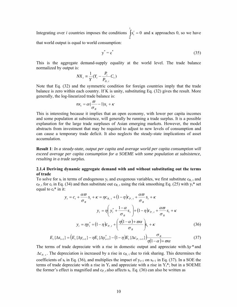
This is interesting because it implies that an open economy, with lower per capita incomes and some population at subsistence, will generally be running a trade surplus. It is a possible explanation for the large trade surpluses of Asian emerging markets. However, the model abstracts from investment that may be required to adjust to new levels of consumption and can cause a temporary trade deficit. It also neglects the steady-state implications of asset accumulation. Result 1: In a steady-state, output per capita and average world per capita consumption will exceed average per capita consumption for a SOEME with some population at subsistence, resulting in a trade surplus. 2.1.4 Deriving dynamic aggregate demand with and without substituting out the terms of trade To solve for st in terms of endogenous yt and exogenous variables, we first substitute cR, t and cP, t for ct in Eq. (34) and then substitute out cR, t using the risk smoothing Eq. (25) with yt* set equal to ct* in it:

( ) κσαϖηηκ

σαϖ

++−+=++= tR

tPtRtR

tt sccscy ,, 1

( ) κσαϖη

σαη ++−+⎟⎟

⎠

⎞⎜⎜⎝

⎛ −+= t

RtPt

Rtt scsyy ,* 11

( ) ( ) κσ

ϖααηηη +⎟⎟⎠

⎞⎜⎜⎝

⎛ +−+−+= t

RtPtt scyy 11 ,

* (36)

( )( ) ( ) ϖααησ

ηη+−

∆−−∆−∆=∆ ++++ 11 1,

*111

RtPttttttt cEyEyEsE (37)

The terms of trade depreciate with a rise in domestic output and appreciate with *y∆ and

tPc ,∆ . The depreciation is increased by a rise in cR, t due to risk sharing. This determines the coefficients of st in Eq. (36), and multiplies the impact of yt+1 on st+1 in Eq. (37). In a SOE the terms of trade depreciate with a rise in Yt and appreciate with a rise in Yt*; but in a SOEME the former’s effect is magnified and cP, t also affects st. Eq. (36) can also be written as

11

DtPt

tt CY

YS σηη )( 1

,* −=

Which compares with the result for a SOE in the Appendix and clearly shows the multiplier

factor ( )( )ϖααησ

σ+−

=1

RD .

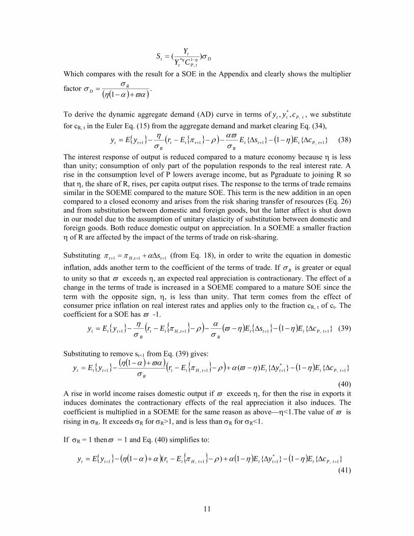
To derive the dynamic aggregate demand (AD) curve in terms of tPtt cyy ,

* ,, , we substitute for cR, t in the Euler Eq. (15) from the aggregate demand and market clearing Eq. (34),

( ) ( ) 1 1,111 ++++ ∆−−∆−−−−= tPtttR

tttR

tt cEsEEryEy ησαϖρπ

ση (38)

The interest response of output is reduced compared to a mature economy because η is less than unity; consumption of only part of the population responds to the real interest rate. A rise in the consumption level of P lowers average income, but as Pgraduate to joining R so that η, the share of R, rises, per capita output rises. The response to the terms of trade remains similar in the SOEME compared to the mature SOE. This term is the new addition in an open compared to a closed economy and arises from the risk sharing transfer of resources (Eq. 26) and from substitution between domestic and foreign goods, but the latter affect is shut down in our model due to the assumption of unitary elasticity of substitution between domestic and foreign goods. Both reduce domestic output on appreciation. In a SOEME a smaller fraction η of R are affected by the impact of the terms of trade on risk-sharing. Substituting 11,1 +++ ∆+= ttHt sαππ (from Eq. 18), in order to write the equation in domestic inflation, adds another term to the coefficient of the terms of trade. If Rσ is greater or equal to unity so that ϖ exceeds η, an expected real appreciation is contractionary. The effect of a change in the terms of trade is increased in a SOEME compared to a mature SOE since the term with the opposite sign, η, is less than unity. That term comes from the effect of consumer price inflation on real interest rates and applies only to the fraction cR, t of ct. The coefficient for a SOE has ϖ -1.

( ) ( ) ( ) 1 1,11,1 ++++ ∆−−∆−−−−−= tPtttR

tHttR

ttt cEsEEryEy ηηϖσαρπ

ση (39)

Substituting to remove st+1 from Eq. (39) gives:

( )( ) ( ) ( ) 1)(11,

*11,1 ++++ ∆−−∆−+−−

+−−= tPttttHtt

Rttt cEyEEryEy ηηϖαρπ

σϖααη

(40) A rise in world income raises domestic output if ϖ exceeds η, for then the rise in exports it induces dominates the contractionary effects of the real appreciation it also induces. The coefficient is multiplied in a SOEME for the same reason as above—η<1.The value of ϖ is rising in σR. It exceeds σR for σR>1, and is less than σR for σR<1. If σR = 1 thenϖ = 1 and Eq. (40) simplifies to:

( )( ) ( ) ( ) 11)(1 1,

*11,1 ++++ ∆−−∆−+−−+−−= tPttttHtttt cEyEEryEy ηηαρπααη

(41)

12

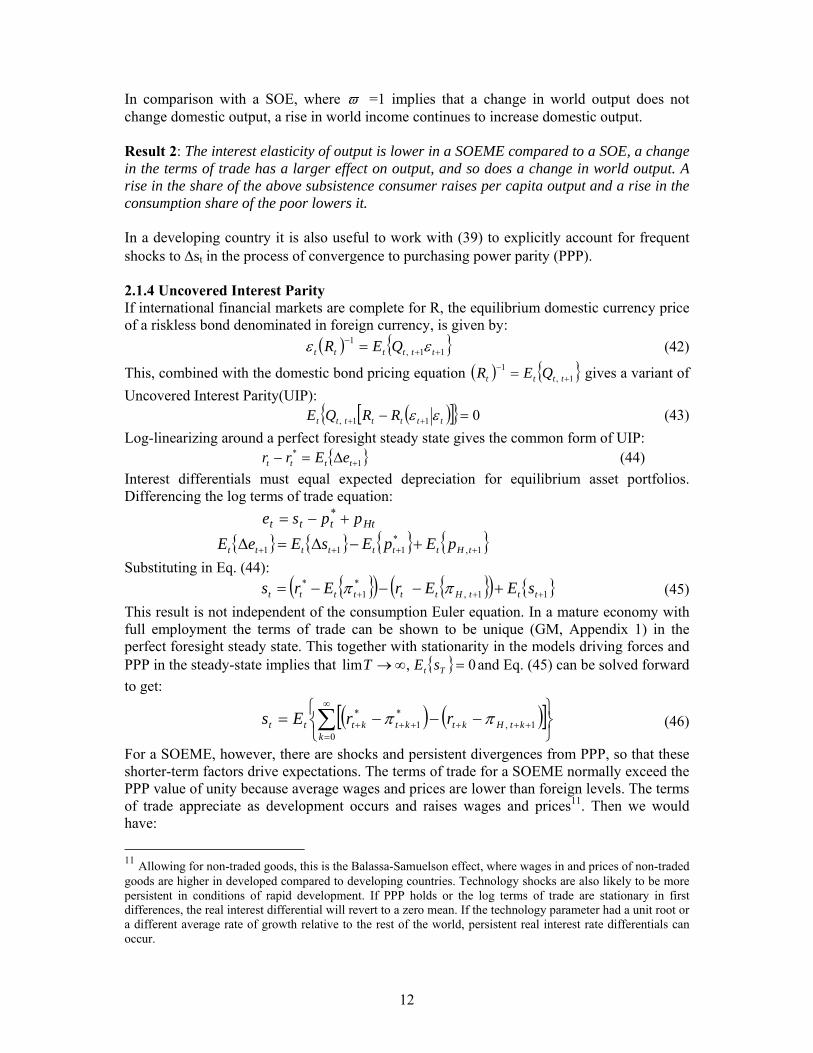
In comparison with a SOE, where ϖ =1 implies that a change in world output does not change domestic output, a rise in world income continues to increase domestic output. Result 2: The interest elasticity of output is lower in a SOEME compared to a SOE, a change in the terms of trade has a larger effect on output, and so does a change in world output. A rise in the share of the above subsistence consumer raises per capita output and a rise in the consumption share of the poor lowers it. In a developing country it is also useful to work with (39) to explicitly account for frequent shocks to ∆st in the process of convergence to purchasing power parity (PPP). 2.1.4 Uncovered Interest Parity If international financial markets are complete for R, the equilibrium domestic currency price of a riskless bond denominated in foreign currency, is given by:

( ) 11,1

++− = tttttt QER εε (42)

This, combined with the domestic bond pricing equation ( ) 1,1

+− = tttt QER gives a variant of

Uncovered Interest Parity(UIP): ( )[ ] 011, =− ++ ttttttt RRQE εε (43)

Log-linearizing around a perfect foresight steady state gives the common form of UIP: 1

*+∆=− tttt eErr (44)

Interest differentials must equal expected depreciation for equilibrium asset portfolios. Differencing the log terms of trade equation:

Htttt ppse +−= * 1,

*111 ++++ +−∆=∆ tHttttttt pEpEsEeE

Substituting in Eq. (44): ( ) ( ) 11,

*1

*+++ +−−−= tttHtttttt sEErErs ππ (45)

This result is not independent of the consumption Euler equation. In a mature economy with full employment the terms of trade can be shown to be unique (GM, Appendix 1) in the perfect foresight steady state. This together with stationarity in the models driving forces and PPP in the steady-state implies that 0,lim =∞→ Tt sET and Eq. (45) can be solved forward to get:

( ) ( )[ ]⎭⎬⎫

⎩⎨⎧

−−−= ∑∞

=++++++

01,

*1

*

kktHktktkttt rrEs ππ (46)

For a SOEME, however, there are shocks and persistent divergences from PPP, so that these shorter-term factors drive expectations. The terms of trade for a SOEME normally exceed the PPP value of unity because average wages and prices are lower than foreign levels. The terms of trade appreciate as development occurs and raises wages and prices11. Then we would have:

11 Allowing for non-traded goods, this is the Balassa-Samuelson effect, where wages in and prices of non-traded goods are higher in developed compared to developing countries. Technology shocks are also likely to be more persistent in conditions of rapid development. If PPP holds or the log terms of trade are stationary in first differences, the real interest differential will revert to a zero mean. If the technology parameter had a unit root or a different average rate of growth relative to the rest of the world, persistent real interest rate differentials can occur.

13

( ) ( )[ ]⎭⎬⎫

⎩⎨⎧

−−−=∆ ∑∞

=+++++++

0

*1

*1,1

kktktktHkttt rrEs ππ

( ) ( )[ ]⎭⎬⎫

⎩⎨⎧

−−−= ∑∞

=++++++

0

*11,

*

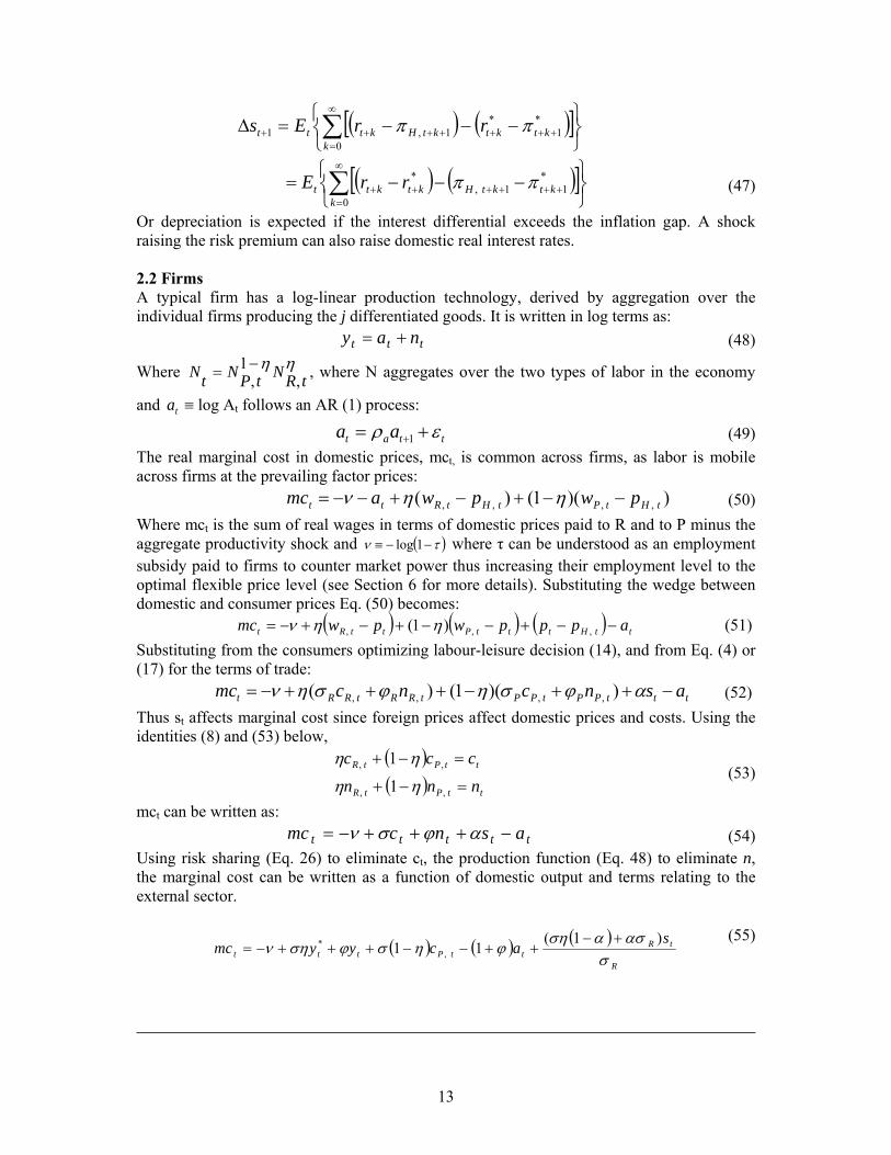
kktktHktktt rrE ππ (47)

Or depreciation is expected if the interest differential exceeds the inflation gap. A shock raising the risk premium can also raise domestic real interest rates. 2.2 Firms A typical firm has a log-linear production technology, derived by aggregation over the individual firms producing the j differentiated goods. It is written in log terms as:

ttt nay += (48)

Where ηηtRNtPNtN ,

1,−= , where N aggregates over the two types of labor in the economy

and ta ≡ log At follows an AR (1) process:

ttat aa ερ += +1 (49) The real marginal cost in domestic prices, mct, is common across firms, as labor is mobile across firms at the prevailing factor prices:

))(1()( ,,,, tHtPtHtRtt pwpwamc −−+−+−−= ηην (50) Where mct is the sum of real wages in terms of domestic prices paid to R and to P minus the aggregate productivity shock and ( )τν −−≡ 1log where τ can be understood as an employment subsidy paid to firms to counter market power thus increasing their employment level to the optimal flexible price level (see Section 6 for more details). Substituting the wedge between domestic and consumer prices Eq. (50) becomes:

( ) ( ) ( ) ttHtttPttRt apppwpwmc −−+−−+−+−= ,,, )1( ηην (51) Substituting from the consumers optimizing labour-leisure decision (14), and from Eq. (4) or (17) for the terms of trade:

tttPPtPPtRRtRRt asncncmc −++−+++−= αϕσηϕσην ))(1()( ,,,, (52) Thus st affects marginal cost since foreign prices affect domestic prices and costs. Using the identities (8) and (53) below,

( )( ) ttPtR

ttPtR

nnn

ccc

=−+

=−+

,,

,,

1

1

ηη

ηη (53)

mct can be written as: ttttt asncmc −+++−= αϕσν (54)

Using risk sharing (Eq. 26) to eliminate ct, the production function (Eq. 48) to eliminate n, the marginal cost can be written as a function of domestic output and terms relating to the external sector.

( ) ( ) ( )R

tRttPttt

sacyymc

σασαση

ϕησϕσην)1(

11 ,* +−

++−−+++−= (55)

14

The intertemporal consumption elasticity of P can be expected to be so low that it is approximately zero. Eq. (8) implies that if 1/σP = 0, then σ = σR /η. The opposite ratio appears in Eq. (39) as the intertemporal elasticity of consumption in the SOEME. On doing this substitution, the coefficient of st in (55) collapses to unity, same as for the SOE. The equivalent relationship for a mature economy (GM Eq. 33) is:

( ) ttttt asyymc ϕϕσν +−+++−= 1* (56) Comparing the two:

(i) The only change in the equation is that the effect of yt* on marginal cost is reduced, but that reduction is compensated by cP, t now increasing marginal cost due to the necessity of maintaining the consumption of P.

(ii) Since P have a highly elastic labour supply, average ϕ is lower so the slope is reduced, and so is the effect of at in shifting marginal cost. The lower response of wage costs to a rise in output is a key difference. Appreciation increases marginal cost as in the SOE.

(iii) Although the effect of st is not changed (the coefficient is decreased if σP>0), st itself may be more volatile since the SOEME may be far from PPP, and there may be more shocks to risk premia, because of greater uncertainty regarding fundamentals.

From Eq. (37) ( )

( ) ϖααηκηησ

+−

−−−−=

1)1( ,

*tPttR

t

cyys , and we define

( )( ) ϖααη

ασαησση +−

+−=

11 R ,

and ( )( )ϖααησ

σ+−

=1

RD . If 1/σP = 0, then σ = σR/η and ση = σD. It also follows that ση<σ.

Both rise as η falls or the proportion of P, who have a very low intertemporal elasticity of consumption (1/σP = 0), rises. As α falls ση rises, and as α approaches 0, or the economy becomes closed, ση equals σ, which is its upper bound. In a fully open economy α approaches unity, and ση falls to its lower bound, which is unity. In a populous developing country that has recently opened out, it is likely that α < η. Substituting Eq. (37) to eliminate st marginal cost becomes:

( ) ( ) ( )( ) ( ) ttPtntt acyymc ϕκσσσηϕσσσην ηηη +−−−−+++−+−= 11 ,* (57)

If σR =1, ϖ =1, ση=1/(η(1-α)+ α). The slope is σα + ϕ for a mature SOE where

( ) ϖαασ

σα +−=

1R , σR enters σα since R in the SOEME are identical to the representative

SOE consumer. Marginal cost for a SOE has σα instead of ση. The slope of marginal cost in the SOEME can be higher since ση > σα, although ϕ is lower for the SOEME. While σα =1 as σR =1, ση always exceeds unity if α <1. Similar results hold for the more general case of σR ≠ 1, as shown below. At α =1, ση = σα, but elsewhere, ση > σα. As α rises towards unity, ση falls to unity and σα rises to unity. The range of possible values is also much higher for ση, since the lower limit is unity when α =1, and the upper limit when α =0 is given by σ. The latter equals σR for the SOE but σR/η for the SOEME and the latter can be very large for low η. Table 1 gives some values for a range of parameters. Since ση is very large for low η and for low α, a SOEME which is not very open and the majority of whose population is poor will have a steep

15

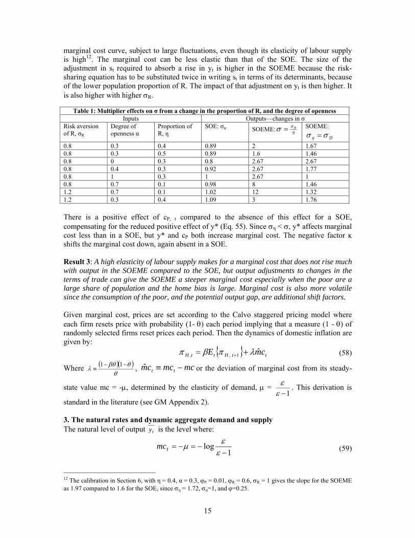
marginal cost curve, subject to large fluctuations, even though its elasticity of labour supply is high12. The marginal cost can be less elastic than that of the SOE. The size of the adjustment in st required to absorb a rise in yt is higher in the SOEME because the risk-sharing equation has to be substituted twice in writing st in terms of its determinants, because of the lower population proportion of R. The impact of that adjustment on yt is then higher. It is also higher with higher σR.

Table 1: Multiplier effects on σ from a change in the proportion of R, and the degree of openness Inputs Outputs—changes in σ

Risk aversion of R, σR

Degree of openness α

Proportion of R, η

SOE: σα SOEME: ησσ R= SOEME:

Dσση =

0.8 0.3 0.4 0.89 2 1.67 0.8 0.3 0.5 0.89 1.6 1.46 0.8 0 0.3 0.8 2.67 2.67 0.8 0.4 0.3 0.92 2.67 1.77 0.8 1 0.3 1 2.67 1 0.8 0.7 0.1 0.98 8 1.46 1.2 0.7 0.1 1.02 12 1.32 1.2 0.3 0.4 1.09 3 1.76 There is a positive effect of cP, t compared to the absence of this effect for a SOE, compensating for the reduced positive effect of y* (Eq. 55). Since ση < σ, y* affects marginal cost less than in a SOE, but y* and cP both increase marginal cost. The negative factor ĸ shifts the marginal cost down, again absent in a SOE. Result 3: A high elasticity of labour supply makes for a marginal cost that does not rise much with output in the SOEME compared to the SOE, but output adjustments to changes in the terms of trade can give the SOEME a steeper marginal cost especially when the poor are a large share of population and the home bias is large. Marginal cost is also more volatile since the consumption of the poor, and the potential output gap, are additional shift factors. Given marginal cost, prices are set according to the Calvo staggered pricing model where each firm resets price with probability (1- θ) each period implying that a measure (1 - θ) of randomly selected firms reset prices each period. Then the dynamics of domestic inflation are given by:

ttHttH cmE ˆ1,, λπβπ += + (58)

Where ( )( )θ

θβθλ

−−≡

11 , mcmccm tt −≡ˆ or the deviation of marginal cost from its steady-

state value mc = -µ, determined by the elasticity of demand, µ = 1−ε

ε . This derivation is

standard in the literature (see GM Appendix 2). 3. The natural rates and dynamic aggregate demand and supply The natural level of output ty is the level where:

1log

−−=−=

εεµtmc (59)

12 The calibration in Section 6, with η = 0.4, α = 0.3, ϕP = 0.01, ϕR = 0.6, σR = 1 gives the slope for the SOEME as 1.97 compared to 1.6 for the SOE, since ση = 1.72, σα=1, and ϕ=0.25.

16

Setting µ−=tmc in (57) and solving for y gives ty : ( ) ( ) ( )( )

κϕσ

σϕσσση

ϕσϕ

ϕσσση

ϕσµν

η

η

η

η

ηη

η

η ++

+

−−−

++

++

−−

+−

= tPttt cayy ,* 11 (60)

Let ϕσϕσ

µν

ηη +=

+−

=Ω1, d ,

( )ϕσϕ

η ++

=Γ1

, ( )dησση −=Ψ , ( )( )( )ησση −−=Σ 1d (61)

So (60) can be written as: κσηdcyay tPttt +Σ−Ψ−Γ+Ω= ,

* (62) As in the case for marginal cost, the natural output for a SOE has σα instead of ση and no cP, t and ĸ term. Since σ > ση > σα, but σR < σα when σR <1, y* always has a negative effect on potential output in the SOEME, but has a positive effect in the SOE when σR <1. The negative effect in the SOEME is reduced by the larger ση. The impact of technology on ty is also reduced but remains positive. The ĸ approximation counters the negative effect of cP, t on

ty , since its coefficient would be larger than that of cP, t on realistic calibration. Potential is higher with higher ĸ to the extent that underdevelopment signifies an unrealized potential. As development occurs and the potential is realized ĸ goes to zero. Result 4: Per capita consumption levels that are below world levels imply higher potential output for a SOEME, but the consumption of the poor reduces it. The negative effect of world output and the positive effect of technology shocks on potential output are reduced in a SOEME compared to a SOE. The domestic output gap xt is defined as the difference of output from capacity, tt yy − :

ttt yyx −≡ (63) Solving for yt from the marginal cost Eq. (57) and using ty from Eq. (60), the difference between the two gives the output gap. The difference arises since marginal cost is set at -µ in deriving ty .

( ) tt

ttttt

xcm

cmmcmcyy

ϕσ

ϕσϕσµ

ϕσµν

ϕσν

η

ηηηη

+=

+=

++

=+−

−+

+=−

ˆ

ˆ (64)

Therefore the inflation dynamics Eq. (58) can be written as, ttHtH xE ηκπβπ += +1, (65)

where ( )ϕσλκ ηη += . This is the dynamic aggregate supply (AS). The slope for a closed economy is λ(σ + ϕ) and for a SOE is λ(σα + ϕ). The slope is reduced in an open compared to a closed economy since σ > ση > σα, but since the gap between σ and ση is large and varying, the slope for the SOEME remains larger than in the SOE. Result 5: The slope of the aggregate supply curve is lower in an open compared to a closed economy but the SOEME curve is normally steeper than the SOE curve when the terns of trade are substituted out.

17

The dynamic aggregate demand (AD) equation for the open economy can be written in terms of the output gap, using the dynamic AD Eq. (42), technology shock Eq. (49) and the equation for ty (62) (see Appendix for derivation):

( )ttHttD

ttt rrErxEx −−−= ++ 1,11 πσ

(66)

Where ( ) ( ) ( ) 11 *11, ++ ∆Ψ−Θ+∆Φ+−−−Γ−= ttDtPtDtaDt yEcEarr σησρσρ

and ( )( )ϖααησσ

+−= 111

RD

, ( )ηϖα −=Θ ,( )( )

ϕσ

σση

η

η

+

−−=Φ

1

Since σD > σα, the output gap, just like output, is less responsive to the interest rate in the SOEME compared to the SOE. In the open economy the natural interest rate rr t is increased by a change in *

ty but the increase is moderated by the negative term ψ, the coefficient of *ty

itself is positive if *ty follows a less than fully persistent autoregressive term such as

yttyt yy ερ +=+ ** 1 with ρy<1. On substituting *ty for the change in *

ty the coefficient

becomes negative. In the SOEME compared to the SOE, change in cP, t decreases trr and so does the level of cP, t if it is growing over time. This is possible if the opportunity cost and therefore wages of labour as productivity rises in informal employment. Technology shocks may be larger in the SOEME and also decrease trr . Result 6: The output gap is less responsive to the interest rate in the SOEME compared to the SOE. Change in consumption of the poor reduces the natural interest rate, while the negative effect of technology shocks and change in world output is intensified in a SOEME compared to a SOE. Since st and its expected value can be more volatile in a SOEME, it is useful to obtain the dynamic AD Eq. (66)’ without substituting out the terms of trade. This is derived in the Appendix, working with Eq. (39) instead of Eq. (42).

[ ]ttHttD

tt rrErxEx −−′

−= ++ 1,11 πσ

(66)’

Where, ( ) ( ) ( ) $11' 11,

*1 +++ ∆+Λ′−∆Φ′+−′−∆Ψ′′−−Γ′−= ttDtPtDttDtaDt sEcEyEarr σησσρσρ

RD ση

σ=

′1

, ( )Rσηϖα −

=Λ , ( )( )

ϕσασαησ

R

R+−=

1$ , and the other dashed parameters are defined

in the Appendix. The comparisons are similar to those for Eq. (66), except that now a rise in y* unambiguously lowers trr , and an expected depreciation in the terms of trade raises trr while an expected appreciation lowers it. Therefore to the extent divergence from PPP and positive risk premiums imply st is more depreciated, expected appreciation during the transition to a SOE implies lower trr and therefore rt. To the extent the transition is not smooth and is interrupted by shocks and jumps in the risk premium, interest rates would rise. The inflation dynamics Eq. (58) now is:

18

tt xcm ϕ=′ˆ (64)’

ttHttH xE ηκπβπ ′+= +1,, (65)’

The slope, λϕκη =′ , is now lower. Result 7: When st is not substituted out the slope of the aggregate supply curve is lower. An expected appreciation in the terms of trade reduces trr while the negative coefficients of the other arguments are increased. Setting yy t= in Eq. (37), which gives the variables influencing st, we can derive the natural

rate of the terms of trade ts . Write Eq. (37) as:

( ) κηησ

−−−−= tPtttD

cyys ,* 11

Substitute for yy t= from Eq. (62), to get: ( ) ( ) ( )( )κσηησ ηdcyas tPttDt −−−+Σ−+Ψ−Γ+Ω= 11 ,

*

The first two terms are similar to a SOE and raise ts , y* also always exerts a negative effect on ts . Negative effects are enhanced by the negative cP, t and κ (since 1 > dση) terms, and multiplied by the fact that σD > σα, the latter being the value in the SOE. The result follows since the cP, t and κ terms capture the lack of maturity of the SOEME, and imply that ts is relatively depreciated compared to the value it will have when the cP, t and κ terms disappear and the SOEME has become a SOE. The steady state natural terms of trade must be appreciated compared to their value when the consumption gap κ is positive since of underdevelopment. The cP, t and κ terms capture the distance from world consumption levels that has to be overcome in the steady-state. Result 8: A technology shock depreciates and a world output appreciates the natural terms of trade in a SOEME as in a SOE, but the coefficients in the SOEME are larger. Increase in the consumption levels of the poor, and reduction of the consumption gap between the SOEME and the SOE both imply an appreciation of the natural terms of trade. 4. Some modifications SOEME’s are often highly dependent on intermediate goods import, and their prices are a major component of inflation. These can be brought in most simply by distinguishing between gross output, y t

G, and value added, yt. Gross output uses imported intermediate inputs, mt, in the share h, while home production continues to be either consumed or exported13.

( ) ttGt mhhnay −++= 1

Optimal pricing (64)’ now becomes: ( ) *1ˆ mttmtmttt ehxhcm πππϕ +∆=−+=′

So that intermediate imports are another factor shifting the AS. Empirical estimation has found that some backward-looking behaviour is important in AS. This is particularly so in 13 Fraga et. al (2004) use a formulation where the SOEME imports only intermediates and exports consumer goods. Therefore no distinction is possible between domestic and consumer inflation. Our distinction between gross output and value added allows that distinction as well as direct cost-push from intermediate goods prices.

19

SOEME’s where many prices are administered (Fraga et. al., 2004). AS Eq. (65)’ can be made to accommodate such behaviour by imposing a share γb of lagged prices:

1ˆ 1,1,, =++′+= −+ bftHbttHtftH cmE γγπγλπβγπ 5. Stability and policy response Pervasive forward-looking behaviour can easily imply instability and multiple equilibria. But it turns out that an adequate policy response can impose stability. This is shown below. First stability conditions are derived, using the AD and AS Eqs. (65) and (66):

ttHttH xE ηκπβπ += +1,, (65)

( )ttHttD

ttt rrErxEx −−−= ++ 1,11 πσ

(66)

Full stabilisation implies that 0, == tHtx π , tttt rrrandyy == . Substituting Eq.(66) in Eq.(65) to write it as a function of xt+1 the two equations become:

1,1

1 +−

+ += tHtDttt ExEx πσ

( ) 1,1

1, +−

+ ++= tHtDtttH ExE πκσβκπ ηη In matrix form they are:

with ⎥⎥⎦

⎤

⎢⎢⎣

⎡

+= −

−

1

11

D

DoA

κσβκσ

η

Since the determinant and trace of the coefficient matrix Ao are both greater than zero the system is unstable. Local indeterminacy is possible and sunspot fluctuations can occur. Now consider a simple policy rule whereby the interest rate is raised if there is domestic inflation, or the output gap is positive:

txthtt xrrr φπφπ ++= ,

Substituting for rt minus its equilibrium value from the rule into Eq. 66, setting πht = πt, and substituting for πt, then substituting for xt in Eq. 65, we get:

( ) 111 +++ −+=++ ttttttDtxD EExEx πβφπσκφφσ πηπ (67)

( ) ( ) 11 )( ++ +++=++ ttxDttDtxD ExE πφσβκσκπκφφσ ηηηπ (68) The two equations now are (67) and (68), which written in matrix form are:

⎥⎦

⎤⎢⎣

⎡=⎥

⎦

⎤⎢⎣

⎡

+

+

1

1

tt

ttT

t

t

ExE

Ax

ππ where ( )⎥⎦

⎤⎢⎣

⎡++

−

Ω=

xDD

DTA

φσβκκσβφσ

ηη

π11 and Π++

=Ωφφσ ηkxD

1

The stability condition for a unique non-explosive solution is14 ( ) ( ) 011 >−+− xφβφκ πη GM have the same result, only the coefficient values are different. Their κ becomes κη or '

ηκ

here; σα in the SOE becomes σD or Dσ ′ here (the latter when st is not substituted out), rr t is also different.

14 The stability condition for a two equation difference system is determinant A > 0, and determinant A+ trace A>-1 when the system is written in the form ...........)( 1 += +tt zEz (see Woodford, 2003).

⎥⎦

⎤⎢⎣

⎡=⎥

⎦

⎤⎢⎣

⎡

+

+

1

1

tt

tto

t

t

ExE

Ax

ππ

20

For stability the policy response to inflation must exceed unity. The reason is that since sticky prices are set in a forward-looking manner, an early and robust policy response will prevent inflationary expectations entering this price setting and therefore lower inflation and the future costs of disinflating (Clarida et.al. 1999). 6. Optimal policy Simulations can give an idea of the optimizing model dynamics, when the central bank minimizes a standard quadratic loss function subject to the AD and AS curves. We test if the impulse responses from a calibrated version of the basic model give results expected in line with theory, and if so examine the relative effectiveness of different kinds of monetary targeting, and contrast the results with those for a mature SOE. The AD and AS equations have the same basic structure under all the different cases they are derived for, only the parameters differ. We calibrate a simple version where the natural interest rate is kept fixed at ρ = β-1-1, and only the forward-looking AD and AS with the derived structural coefficients, uncovered interest parity, and the policy reaction function are simulated. The calibration is loosely based on Indian stylized facts. Since empirical estimations and the dominance of administered pricing in SOEME’s suggest that past inflation affects current inflation, the modification of the AS developed in Section 4 is used, with γb set at 0.2 so γf is 0.8, in most simulations. The openness coefficient α is set at 0.3; the proportion of R,15 η at 0.4; β= 0.99 implies a riskless annual steady-state return of 4 percent; the price response to output, ϕ, is set at 0.25, which implies an average labour supply elasticity of 4. Initial conditions are normalized at unity so the log value is zero. GM (Section 4) show the natural output y t can be optimally equivalent to a flexible price equilibrium, if the subsidy ν is set so as to correct for market power. If mc = - µ , and ε is the

elasticity of demand, setting τ such that ( )( )ε

ατ 1111 −=−− or ( )αµν −+= 1log where

( )τν −−= 1log gives the equivalent of the optimal flexible price equilibrium. In a SOEME it is also necessary to correct for deviations of st, and other distortions from consumption inequality. An elasticity of substitution between differentiated goods, ε equal to 6, implies a steady-state mark-up, µ, of 1.2. The subsidy to deliver the flexible price equilibrium ν then equals µ - 0.1579. The price setting parameters are such that prices adjust in an average of one year (θ =0.75), giving λ = 0.24. Since σR = 1 and 1/σP=0, the implied average intertemporal elasticity of substitution is η(1-α) + α=0.58. A negative interest rate effect on consumption requires an intertemporal elasticity large enough to so that the substitution effect is higher than the positive income effect of higher interest rates on net savers. Empirical studies have found real interest rates to have weak effects on consumption. Especially in low-income countries subsistence considerations are stronger that intertemporal factors. This is particularly so when the share of food in total expenditure is large. The elasticity Ogaki, Ostry and Reinhart (1996) estimate

15 GMM regressions of CPI inflation for India (Goyal, 2005) give a coefficient of expected inflation of 0.67. India’s share of imports in GDP was about 20 percent in 2005, and the proportion of population in rural areas 60 percent. In GMM regressions of aggregate demand with monthly data, the one period forward index of industrial production was strongly significant with a coefficient of –0.42.

21

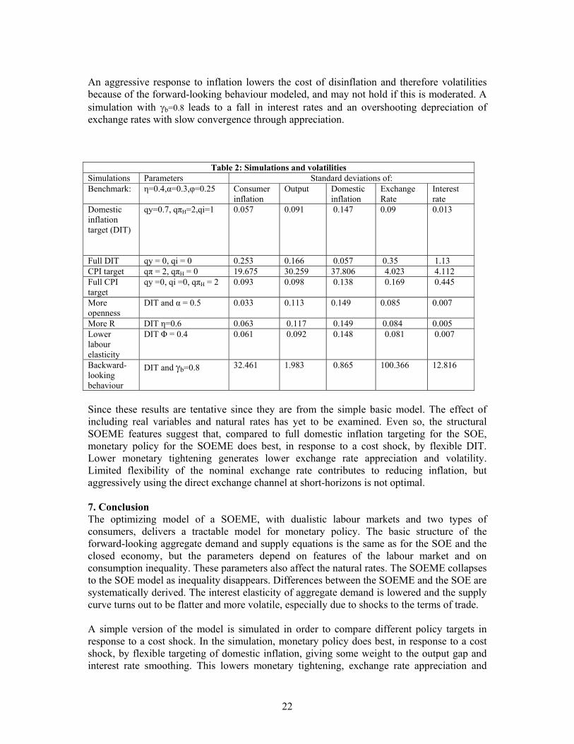
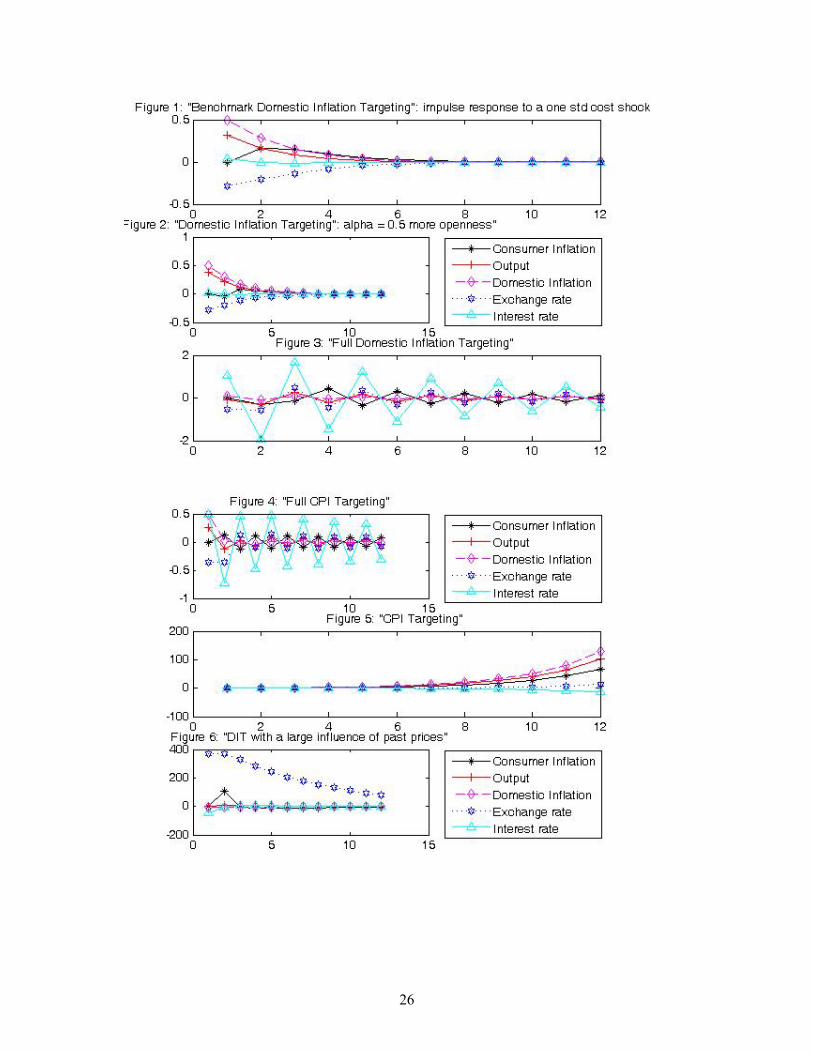
in a large cross-country study, varies from 0.05 for Uganda and Ethiopia to a high of 0.6 for Venezuela and Singapore. Our average elasticity compares well with these figures. Since cost shocks are frequent in SOEMEs the exogenous driving force simulated is a unit standard deviation cost shock to period one domestic inflation. The policy response is obtained under discretion with a central bank minimizing different weighted averages of inflation (domestic or consumer), output gap and interest rate deviations from equilibrium. Under strict inflation targeting a weight of 2 is given only to inflation. The exchange rate directly affects consumer inflation while it affects domestic inflation through its affect on marginal cost. Monetary policy affects domestic inflation directly by changing the output gap; domestic inflation is a component of consumer inflation. Table 2 reports some of the simulations done, where the qs are the weights attached to the different arguments of the loss function (The weights are calculated according to the optimal values derived in GM). The benchmark set of parameters for which sensitivity analysis is undertaken are indicated. A high weight is always given to inflation, in line with the stability arguments of section 5. The square of the standard deviations reported in Table 2 give a measure of the welfare loss. The policy response is on expected lines. The impulse responses show a nominal appreciation and a rise in interest rates covering the expected future depreciation in response to the cost shock (Figures 1, 2, 3, 4). There is stability or convergence back to the initial state over the 12 periods of the simulation except under consumer price inflation (CPI) targeting when the positive weight on output gap and interest smoothing leads to an initial fall in interest rates and a subsequent rise in inflation and the output gap (Figure 5). The strict inflation targeting regimes are all stable, although both full CPI and domestic inflation targeting (DIT) by inducing large initial rise in interest rates and appreciation result in decaying cycles. Theory suggests that full DIT should be optimal when the correction ν is made for sticky prices (GM). Variations in exchange rates compensate for sticky prices. But in a SOEME there are other distortions, for example, consumption inequality. Therefore it is not surprising that flexible DIT which raises the initial interest rate the least and has a small initial appreciation delivers the least volatility (Table 2), performing the best of all the alternatives. In the SOEME changes in the terms of trade multiply the required income response and make the supply curve steeper, therefore fluctuations in the exchange rate should be reduced, but some fluctuations contribute to reducing inflation through the exchange rate channel so less monetary tightening is required. Full DIT does deliver lower domestic inflation volatility, but, policy needs to lower the output gap to achieve this further reduction in domestic inflation, so more tightening is required, leading to a sharp rise in interest rates. Svensson (2000), in a related model finds that full CPI leads to too large a variation in exchange rates since it uses the direct exchange rate channel at short-horizons to stabilize CPI. He finds that with a loss function that includes more variables that flexible CPI performs best, since it stabilizes the real exchange rate also. But in our model flexible CPI leads to too little monetary tightening in response to inflation, implying unstable divergence over time. Sensitivity analysis with variation in key parameters under CPI has expected results (Table 2 and Figure 2). More openness, a higher proportion of R, and lower labour elasticity lower the initial interest response and volatility. The reason is that all three changes lower the interest elasticity of output and the response of domestic inflation to the output gap. These results are robust for different model structures. A SOE characterized by η=1 would therefore have a lower rise in interest rates and appreciation compared to a SOEME.

22

An aggressive response to inflation lowers the cost of disinflation and therefore volatilities because of the forward-looking behaviour modeled, and may not hold if this is moderated. A simulation with γb=0.8 leads to a fall in interest rates and an overshooting depreciation of exchange rates with slow convergence through appreciation.

Table 2: Simulations and volatilities Simulations Parameters Standard deviations of: Benchmark: η=0.4,α=0.3,φ=0.25 Consumer

inflation Output Domestic

inflation Exchange Rate

Interest rate

Domestic inflation target (DIT)

qy=0.7, qπH=2,qi=1

0.057 0.091 0.147 0.09 0.013

Full DIT qy = 0, qi = 0 0.253 0.166 0.057 0.35 1.13 CPI target qπ = 2, qπH = 0 19.675 30.259 37.806 4.023 4.112 Full CPI target

qy =0, qi =0, qπH = 2 0.093 0.098 0.138 0.169 0.445

More openness

DIT and α = 0.5 0.033 0.113 0.149 0.085 0.007

More R DIT η=0.6 0.063 0.117 0.149 0.084 0.005 Lower labour elasticity

DIT Φ = 0.4 0.061 0.092 0.148 0.081 0.007

Backward-looking behaviour

DIT and γb=0.8 32.461 1.983 0.865 100.366 12.816

Since these results are tentative since they are from the simple basic model. The effect of including real variables and natural rates has yet to be examined. Even so, the structural SOEME features suggest that, compared to full domestic inflation targeting for the SOE, monetary policy for the SOEME does best, in response to a cost shock, by flexible DIT. Lower monetary tightening generates lower exchange rate appreciation and volatility. Limited flexibility of the nominal exchange rate contributes to reducing inflation, but aggressively using the direct exchange channel at short-horizons is not optimal. 7. Conclusion The optimizing model of a SOEME, with dualistic labour markets and two types of consumers, delivers a tractable model for monetary policy. The basic structure of the forward-looking aggregate demand and supply equations is the same as for the SOE and the closed economy, but the parameters depend on features of the labour market and on consumption inequality. These parameters also affect the natural rates. The SOEME collapses to the SOE model as inequality disappears. Differences between the SOEME and the SOE are systematically derived. The interest elasticity of aggregate demand is lowered and the supply curve turns out to be flatter and more volatile, especially due to shocks to the terms of trade. A simple version of the model is simulated in order to compare different policy targets in response to a cost shock. In the simulation, monetary policy does best, in response to a cost shock, by flexible targeting of domestic inflation, giving some weight to the output gap and interest rate smoothing. This lowers monetary tightening, exchange rate appreciation and

23

volatility. Exchange rate flexibility makes a major contribution to reducing inflation, but aggressively using the direct exchange channel at short-horizons to reduce inflation, is not optimal. The stripped down version simulated gives results in line with theory, but much work remains to be done. First, to simulate the full version, obtaining time paths of the natural rates, and the response to other shocks such as demand, technology, and changes in the consumption of P, and to different lag structures. Second, to simulate the version without substituting out the terms of trade. That would reduce the slope of the supply curve but subject it to more shocks. Third, estimations for India (Goyal, 2005) suggest that CPI inflation is forward-looking in India but domestic inflation is not. It will be useful, therefore to simulate the model imposing this restriction. Fourth, the implications of pricing to market or in importer’s currency can also be explored although this may not be so relevant for commodity imports. Including capital markets may imply a greater role for interest smoothing. Fifth, SOEMEs have different kinds of nominal and real wage rigidities. It would be particularly useful to model the consequences of real wages rigid in terms of food prices (Goyal, 2005), since this is a feature of populous low-per capita income SOEMES. Sixth, to explore the consequences of relaxing simplifying assumptions, including on elasticities and on uncorrected steady-state distortions such as deviations from PPP and on asset accumulation through the current account. A non-zero current account implies that multiple steady-states can exist. Seventh, derive optimal weights for the loss function in a SOEME, in order to do welfare analysis. References Clarida, R., Gali, J., and Gertler, M., 1999, ‘The Science of Monetary Policy: A New Keynesian perspective’, Journal of Economic Literature, 37 (4), 1661-707. Clarida, R., Gali, J., and Gertler, M., 2001, ‘Optimal Monetary Policy in Closed Versus Open Economies: An integrated approach’, American Economic Review, 91 (2), May, 248-252. Fraga, A., I. Goldfajn, and A. Minella, 2004, ‘Inflation Targeting in Emerging Market Economies’, in Gertler M. and K. Rogoff (eds.) NBER Macroeconomics Annual, Cambridge: MIT Press. Gali, J. and T. Monacelli, 2005, “Monetary Policy and Exchange Rate Volatility in a Small Open Economy.” Review of Economic Studies, 72(3): 707-734. Goyal, A., 2005, ‘Incentives from Exchange rates in an Institutional Context,’ IGIDR working paper available at www.igidr.ac.in/pdf/publication/WP-2005-002-R1.pdf Obstfeld, M. and K. Rogoff, 1996, Foundations of International Macroeconomics, Cambridge, Massachusetts: MIT Press. Ogaki, Masao, Jonathan Ostry, and Carmen M. Reinhart, 1996, ‘Savings Behaviour in Low-and Middle-Income Countries: A comparison’, IMF Staff Papers 43 (March): 38-71 Stiglitz, J.E., 2007, ‘Remarks on Bank Research Evaluation’ http://siteresources.worldbank.org/DEC/Resources/84797-1109362238001/726454-1164121166494/JES-bankResearchReviewanjesfin.pdf accessed on 12/01/07

24

Svensson, L.E.O, 2000, ‘Open-economy inflation targeting’, Journal of International Economics, 50, 155-183. Woodford, M, 2003, Interest and prices: Foundations of a Theory of Monetary Policy, NJ: Princeton University Press. Appendix Determinants of the terms of trade in a SOE With PPP Eq. (35) can be written as:

**, ttttF CPYP εε =

**, ttttF CPYP =

Then from Eq. (32): ttHttF YPYP ,

*, = (A1)

or *,

,

t

t

tH

tFt Y

YPP

S =≡ (A2)

Alternatively, substituting C* for Ct in Eq. (33), using Eq. (35) to substitute Y* for C* and solving gives A2. To write the dynamic AD in terms of the output gap Writing the dynamic AD, Eq. (40), as:

)1()(11,

*11,1 ++++ ∆−−∆Θ+−−−= tPttttHtt

Dttt cEyEEryEy ηρπ

σ (40)

Substituting the output gap definition, Eq. (63), in (40):

( ) ttttPtttD

tHttD

ttt yyEcEyEErxEx −+∆Ξ−∆Θ++−−= +++++ 11,*

11,111 ρσ

πσ

From Eq. (60) for ty :

1,1*

11 ++++ ∆Φ−∆Γ+∆Ψ−=− tPtttttttt cEaEyEyyE

Also using tat aa )1(1 ρ−−=∆ + since ttat aa ερ +=+1 gives:

( ) ( ) ( ) ( ) ttPtttD

tHttD

ttt acEyEErxEx αρηρσ

πσ

−Γ−∆Φ+−−∆Ψ−Θ++−−= ++++ 1)1(111,

*11,1

From which, the final form. Eq. (66) is derived by defining the natural rate of interest. To derive the dynamic AD without substituting out st We use Eq. (39) instead of Eq. (40),

( ) )1(11,11,1 ++++ ∆−−∆Λ−−−

′−= tPttttHtt

Dttt cEsEEryEy ηρπ

σ (39)

Marginal cost without substituting for st is Eq. (55)

( ) ( ) ( )( )t

R

RttPttt sacyymc

σασαησ

ϕησϕσην+−

++−−+++−=111 ,

* (55)

To solve for ty from (55), set µ−=tmc , and solve for yt:

25

( ) ( ) ( )( )t

R

RttPtt sacyy

ϕσασαση

ϕϕ

ϕησ

ϕση

ϕµν +−

−+

+−

−−−

=111

,*

Writing the parameters as the dashed symbols below:

ttPttt scyay $,* −Φ′−Ψ′−Γ′+Ω′=

Writing the dynamic AD curve in terms of the output gap,

( ) ttttttPtD

tHttD

ttt yyEsEcEErxEx −+∆Λ−∆Σ′−′

+−′

−= ++++ 11,1,111 ρσ

πσ

( ) ,)1(1

1$1,*

11'1,1

1 tPctED

tstEtPctEtytEtatEtHtEtrD

txtEtx ∆−−′

++∆−+∆Φ′−+∆Ψ′−+∆Γ++−′

−+= ηρσ

πσ

Substituting $' 11,*

111 +++++ ∆−Φ′−∆Ψ′−∆Γ=− tttPtttttttt sEcEyEaEyyE gives the final Eq. (66’).

( ) ( ) ( )( )t

R

RttPtt sacyy

σασαση

ϕησσηµνϕ+−

−++−−−−=111 ,

*

26