A general discrete-time modeling framework for animal movement using multistate random walks

Ecological Monographs, 82(3), 2012, pp. 335–349� 2012 by the Ecological Society of America

A general discrete-time modeling framework for animal movementusing multistate random walks

BRETT T. MCCLINTOCK,1,4 RUTH KING,1 LEN THOMAS,1 JASON MATTHIOPOULOS,2 BERNIE J. MCCONNELL,2

AND JUAN M. MORALES3

1Centre for Research into Ecological and Environmental Modelling and School of Mathematics and Statistics,University of St Andrews, St Andrews, Fife, Scotland KY16 9LZ United Kingdom

2Scottish Oceans Institute, School of Biology, University of St Andrews, St Andrews, Fife, Scotland KY16 8LB United Kingdom3Ecotono, INIBIOMA–CONICET, Universidad Nacional del Comahue, Quintral 1250, 8400 Bariloche, Argentina

Abstract. Recent developments in animal tracking technology have permitted thecollection of detailed data on the movement paths of individuals from many species.However, analysis methods for these data have not developed at a similar pace, largely due toa lack of suitable candidate models, coupled with the technical difficulties of fitting suchmodels to data. To facilitate a general modeling framework, we propose that complexmovement paths can be conceived as a series of movement strategies among which animalstransition as they are affected by changes in their internal and external environment. Wesynthesize previously existing and novel methodologies to develop a general suite ofmechanistic models based on biased and correlated random walks that allow differentbehavioral states for directed (e.g., migration), exploratory (e.g., dispersal), area-restricted(e.g., foraging), and other types of movement. Using this ‘‘toolbox’’ of nested modelcomponents, multistate movement models may be custom-built for a wide variety of speciesand applications. As a unified state-space modeling framework, it allows the simultaneousinvestigation of numerous hypotheses about animal movement from imperfectly observeddata, including time allocations to different movement behavior states, transitions betweenstates, the use of memory or navigation, and strengths of attraction (or repulsion) to specificlocations. The inclusion of covariate information permits further investigation of specifichypotheses related to factors driving different types of movement behavior. Using reversible-jump Markov chain Monte Carlo methods to facilitate Bayesian model selection and multi-model inference, we apply the proposed methodology to real data by adapting it to the naturalhistory of the grey seal (Halichoerus grypus) in the North Sea. Although previous grey sealstudies tended to focus on correlated movements, we found overwhelming evidence that biastoward haul-out or foraging locations better explained seal movement than did simple orcorrelated random walks. Posterior model probabilities also provided evidence that sealstransition among directed, area-restricted, and exploratory movements associated with haul-out, foraging, and other behaviors. With this intuitive framework for modeling andinterpreting animal movement, we believe that the development and application of custom-made movement models will become more accessible to ecologists and non-statisticians.

Key words: animal location data; Bayesian model selection; biased correlated random walk; grey seal;Halichoerus grypus; movement model; North Sea; reversible-jump Markov chain Monte Carlo; state-spacemodel; switching behavior; telemetry.

INTRODUCTION

Our ability to track and monitor wildlife populations

has greatly improved with recent technological advance-

ments. These include animal-borne devices that allow

the collection of accurate time series of individual

location data (McConnell et al. 2010, Tomkiewicz et

al. 2010), biotelemetry devices providing physiological

information (Cooke et al. 2004, Payne et al. 2011), and

remote sensing and geographic information system

(GIS) technologies for the acquisition of detailed

landscape data at multiple spatial scales (Gao 2002).

Along with these developments, new challenges have

arisen in the collection, management, and analysis of

georeferenced animal location data (Cagnacci et al.

2010, Urbano et al. 2010).

Although Global Positioning System (GPS) and other

relocation technologies have enabled the collection of

large amounts of animal location data from diverse

terrestrial and aquatic taxa (Tomkiewicz et al. 2010),

model development for the analysis of these data has

lagged behind. This is beginning to change as new

methods continue to appear in the ecological literature

Manuscript received 1 March 2011; revised 22 March 2012;accepted 2 April 2012. Corresponding Editor: K. B. Newman.

4 Present address: National Marine Mammal Laboratory,Alaska Fisheries Science Center, National Marine FisheriesService, NOAA, 7600 Sand Point Way NE, Seattle, Wash-ington 98115 USA. E-mail: [email protected]

335

(Holyoak et al. 2008, Schick et al. 2008), but unlike

many other areas of ecology, no general estimation

framework has been developed for the analysis of

movement trajectories that is widely accepted by the

practitioners collecting the majority of these data sets.

For example, there are well-established inferential

methods in population and community ecology for

examining patterns of abundance (e.g., Otis et al. 1978,

Buckland et al. 2001, Borchers et al. 2002), species

occurrence (e.g., MacKenzie et al. 2006), and related

vital rates that address uncertainties (e.g., imperfect

detection) associated with the process by which the data

were obtained (Williams et al. 2002, King et al. 2009).

There also exists readily accessible software for the

analysis of these data by wildlife professionals (e.g.,

White and Burnham 1999, Thomas et al. 2010). There

remains a similar need (and desire) to develop accessible,

inferential data analysis methods in movement ecology

(Schwarz 2009, Morales et al. 2010).

As animals respond to physiological and environmen-

tal stimuli, they often exhibit different movement

behavior states (or modes). Simple examples include

‘‘exploratory’’ and ‘‘encamped’’ states in elk (Morales et

al. 2004) or, equivalently, ‘‘traveling’’ and ‘‘foraging’’

states in grey seals (Breed et al. 2009), where ‘‘explor-

atory’’ or ‘‘traveling’’ describe movement states associ-

ated with greater directional persistence and velocity

relative to the ‘‘encamped’’ or ‘‘foraging’’ states.

Inferring patterns and dynamics of movement from

time series of animal location data often involves the

estimation of movement parameters associated with

different types of movement behavior states. However,

because these states often cannot be observed directly,

they must be inferred based on trajectories alone in the

absence of ancillary information (but see Discussion).

Estimation is complicated further by the fact that animal

location data often contain considerable observation

error in both time and space, as well as missing (or

intermittent) observations. Sophisticated statistical

models of the underlying movement and observation

process are therefore required to facilitate reliable

inference (Jonsen et al. 2005, Patterson et al. 2008,

Schick et al. 2008).

A variety of approaches for analyzing animal location

data have been proposed in recent years, and these

primarily differ in the spatiotemporal conceptualization

of the movement process. These include discrete-time

and discrete-space (Brownie et al. 1993, Schwarz et al.

1993, Dupuis 1995, King and Brooks 2002), discrete-

time and continuous-space (Morales et al. 2004, Jonsen

et al. 2005), continuous-time and discrete-space (Ovas-

kainen et al. 2008), or continuous-time and continuous-

space (Blackwell 2003, Johnson et al. 2008) movement

process models. Similarly, latent behaviors associated

with different types of movement can be treated as

continuous (Forester et al. 2007) or discrete (Morales et

al. 2004, Jonsen et al. 2005) states among which animals

transition in response to changes in their internal and

external environment. The representation of movement

also differs among these approaches, by specifying the

movement process on the positions themselves (Black-

well 2003, Jonsen et al. 2006) or derived quantities, such

as the differences between consecutive coordinates

(Jonsen et al. 2005, Johnson et al. 2008), step lengths

(Forester et al. 2007), or both step lengths and turning

angles (Morales et al. 2004). Although earlier methods

ignored error in the timing and location of observations

(Blackwell 2003, Morales et al. 2004), most recent

approaches simultaneously model both the movement

process and observation process using state-space

methods (Anderson-Sprecher and Ledolter 1991, Jonsen

et al. 2005, Johnson et al. 2008, Patterson et al. 2008).

The myriad of proposed methodologies for analyzing

movement data makes selection of any particular

method (or model) a difficult task. The most sophisti-

cated continuous-time approaches, although appealing

from a theoretical perspective, are prohibitively techni-

cal for many non-statisticians. Further, continuous-time

and continuous-behavior models are less appealing to

practitioners because the parameters (e.g., instantaneous

diffusion process parameters) can be difficult to interpret

biologically. Discrete-space models often necessitate

spatial resolutions requiring high-dimensional matrices

or integrals that can lead to computational difficulties.

Perhaps most inhibiting to general use by ecologists is

the fact that the majority of movement models

developed to date have focused on species-specific

applications and relatively few behavioral states, with

little scope for generalization. Given these challenges, it

is certainly not surprising that even less attention has

been given to strategies for model selection and multi-

model inference (Hoeting et al. 1999, Burnham and

Anderson 2002, King et al. 2009) in the analysis of

movement data (but see King and Brooks 2002, 2004,

Morales et al. 2004).

We synthesize many of the appealing elements of

previous approaches (e.g., Dunn and Gipson 1977,

Blackwell 1997, 2003, King and Brooks 2002, Morales et

al. 2004, Jonsen et al. 2005, Johnson et al. 2008) in

combination with novel methodologies to formulate a

general modeling strategy for individual animal move-

ment in discrete time and continuous space that can be

readily adapted to accommodate many different types of

movement and behavioral states. With an increased

emphasis on ecological inference from animal location

data, these states can be associated with directed (e.g.,

migratory or evasive), area-restricted (e.g., foraging or

nesting), exploratory (e.g., dispersal or searching), and

correlated movements as dictated by the species and

application of interest. Using Bayesian analysis meth-

ods, we also propose a model selection and multi-model

inference procedure based on weights of evidence for

these different types of movement behaviors. We

demonstrate the use of this mechanistic, inferential

modeling framework by adapting it to the natural

history of the grey seal (Halichoerus grypus) in the North

BRETT T. MCCLINTOCK ET AL.336 Ecological MonographsVol. 82, No. 3

Sea. This apex marine predator often demonstrates

characteristically complex movement patterns among

haul-out colonies and foraging patches.

METHODS

A general model for individual movement in discrete time

We first formulate a general model for animal

movement as a mixture of discrete-time random walks.

An individual may switch among a set of discrete

movement behavior states z¼ 1, . . . , Z, where each state

is characterized by distributions for the step length and

direction (or bearing) of movement between consecutive

positions (Xt�1, Yt�1) and (Xt, Yt) for each time step t¼1, . . . , T. We assume the T time steps are of equal length

(but see State-space formulation). The set of Z move-

ment behavior states can include directed movements

toward particular locations or ‘‘exploratory’’ movements

that are not associated with any particular location.

When these movement behavior states are not directly

observable, this can be viewed as a hidden Markov

model (Zucchini and MacDonald 2009, Langrock et al.

2012).

For flexibility and mathematical convenience, we

follow Morales et al. (2004) by selecting a Weibull

distribution for the step length (st) and a wrapped (w)

Cauchy distribution for the direction (/t) of movement,

but other distributions for step length (e.g., gamma) or

direction (e.g., von Mises) could also be used (Codling et

al. 2010). The movement process model is therefore a

discrete-time, continuous-space, multistate random walk

with step length [st j zt¼ i] ; Weibull(ai, bi ) and direction

[/t j zt ¼ i] ; wCauchy(li, qi ). Specifically, we have the

following probability density functions:

f ðst j zt ¼ iÞ ¼ bi

ai

st

ai

� �bi�1

exp½�ðst=aiÞbi �

and

f ð/t j zt ¼ iÞ ¼ 1

2p1� q2

i

1þ q2i � 2qicosð/t � liÞ

for az . 0, bz . 0, 0 � /t , 2p, 0 � lz , 2p,�1 , qz ,

1, and z ¼ 1, . . . , Z. Assuming independence between

step length and direction within each movement

behavior state (see Discussion), the joint likelihood for

st and /t (conditional on the latent state variable zt) is

f ðs;/ j zÞ ¼YT

t¼1

f ðst j ztÞf ð/t j ztÞ:

For switches between movement behavior states, we

assign a categorical distribution to the latent state

variable zt. The simplest approach assigns every time

step to a movement behavior state independent of

previous states or ancillary information:

zt ; Categoricalðw1; :::;wZÞ

such that

wi ¼ Prðzt ¼ iÞ

where wi is the (fixed) probability of being in state i at

time t, andPZ

i¼1 wi ¼ 1. This assumption is generally

unrealistic for animal movements. Alternatively (and

more realistically), one could incorporate memory into

the state transition probabilities using a jth-order

Markov process. Assuming that movement behavior

states were known, Blackwell (1997, 2003) used a first-

order Markov transition matrix to characterize switches

between states in continuous time. For a first-order

Markov process in discrete time,

½zt j zt�1 ¼ k�; Categoricalðwk;1; :::;wk;ZÞ

and

wk;i ¼ Prðzt ¼ i j zt�1 ¼ kÞ

for k¼1, . . . , Z where wk,i is the probability of switching

from state k at time t – 1 to state i at time t, andPZ

i¼1 wk;i

¼ 1. We note that this Markovian structure is analogous

to the state transition probabilities for multistate

capture–recapture models (e.g., Brownie et al. 1993,

Schwarz et al. 1993).

The multistate movement model is specified according

to the particular species and ecological conditions of

interest. The various movement behavior states may be

solely characterized by biased, correlated, or exploratory

types of movement, but environmental covariates and

alternative parameterizations may also be utilized to

describe the movement process. Below we present a suite

of models for different movement characteristics that

can be combined to form complex movement behavior

states. We emphasize that the proposed models fall

under the same general modeling framework, with the

more basic models remaining nested within the more

complex models. These, and other extensions (see

Discussion), may therefore be thought of as contribu-

tions to a ‘‘toolbox,’’ from which a wide range of

custom-made multistate movement models in discrete

time can be assembled. By adding or removing

components from the toolbox, one may compare the

different models nested within the most general model

(see Example: grey seal movement in the North Sea). This

allows simultaneous investigation of numerous hypoth-

eses about animal movement, including those involving:

(1) time allocations to different movement behavior

states (i.e., ‘‘activity budgets’’); (2) the use of navigation

for directed movement toward specific locations; (3) the

relative strength of bias toward (or away from) specific

locations; (4) the existence of spatially unassociated (but

potentially correlated) exploratory movement states;

and (5) factors affecting transition probabilities between

movement behavior states.

Biased movements.—Biased movement behavior states

exhibiting attraction (or aversion) to particular locations

can be incorporated within the proposed framework.

Suppose the set of Z movement behavior states is

composed entirely of attractions to one of c different

August 2012 337GENERAL FRAMEWORK FOR ANIMAL MOVEMENT

‘‘centers of attraction’’ (i.e., Z¼ c). Assuming movement

at time t is biased toward center of attraction i (i.e., zt¼i ), we calculate the expected movement direction (li,t) as

the direction between the individual’s previous location

(Xt�1, Yt�1) and the location of the center of attraction

(X*i , Y*

i ) at time t. We note that the coordinates of each

center of attraction (X*z , Y*

z ), z ¼ 1, . . . , c, are not

necessarily assumed to be known (see Example: grey seal

movement in the North Sea).

The strength of bias to each center of attraction is

determined by the mean vector length of the wrapped

Cauchy distribution (0 � qz , 1). This strength of bias

need not be constant. For example, in some instances

one may expect less directed movement once an

individual has reached the vicinity of the current center

of attraction, so that we may specify:

qz;t ¼ tanhðrzdtÞ

where dt is some metric of the distance (e.g., Euclidean)

to the current center of attraction, rz � 0 is a (state-

dependent) scaling parameter, and tanh is a hyperbolic

tangent (see Appendix A). As an individual is located

closer to the current center of attraction, qz,t ! 0, and

the movement direction is uniformly distributed on the

unit circle. This allows for unbiased area-restricted

searches (e.g., ‘‘encamped’’ or ‘‘foraging’’ types of

movement; sensu Morales et al. 2004, Breed et al.

2009) once in the vicinity of the current center of

attraction. As an individual is located farther from the

current center of attraction, qz,t ! 1, and /t is not

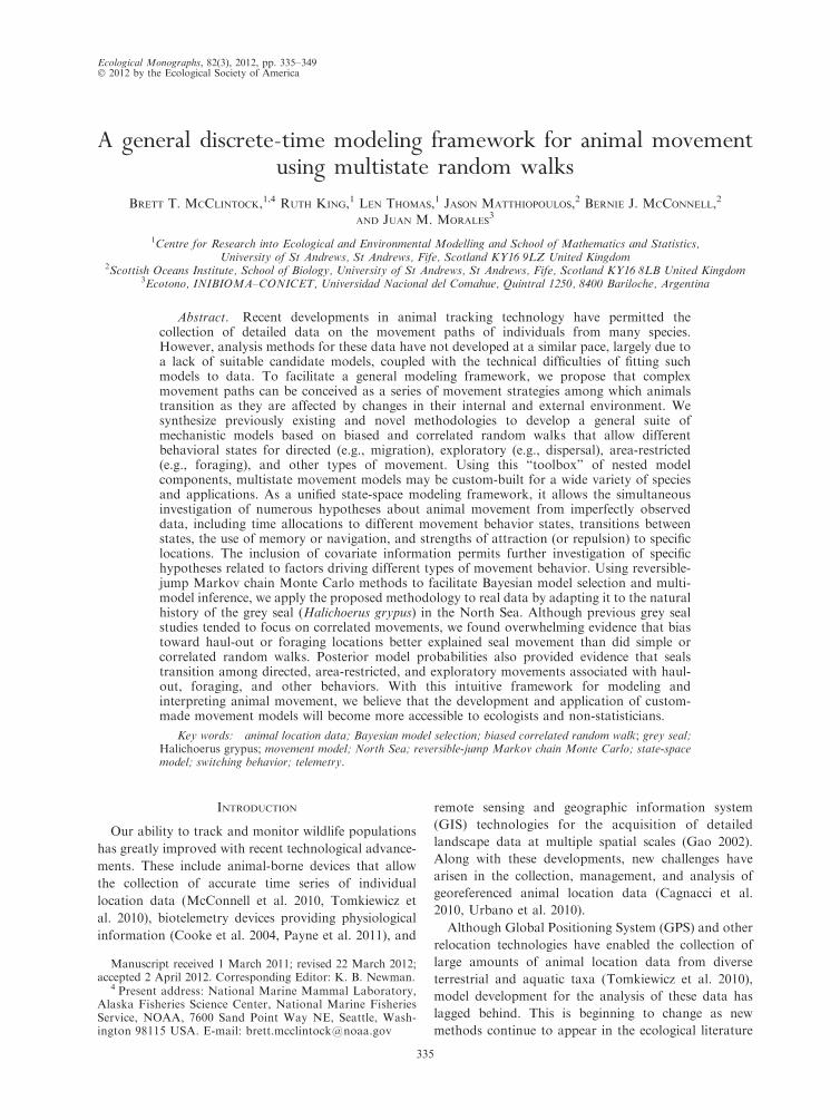
allowed to deviate from lz,t (Fig. 1a). We note that this

formulation also permits bias away from a ‘‘center of

repulsion’’ when �1 , qz � 0.

More complicated structural forms may be utilized for

qz. For example, when far away, an animal may have

only a general sense of the location of a center of

attraction, but the movement direction draws closer to

lz,t as the distance to the center of attraction decreases

(i.e., the individual ‘‘hones in’’ on its target). An

additional quadratic term (qz) allows this type of

behavior to be included in the following model:

qz;t ¼ tanhðrzdt þ qzd2t Þ

where rz and qz are constrained such that qz,t � 0 for all

reasonable dt within the study area. We note that

alternative link functions, such as the logit link, may be

utilized when specifying qz as a function of covariates

(see Example: grey seal movement in the North Sea).

Biased, correlated movements.—Additional structure

can describe biased movement behavior states that

exhibit correlations between successive movement direc-

FIG. 1. Simulated time series of animal location data(position coordinates X and Y ) using three centers of attractionfrom multistate (a) biased random walk, (b) biased correlatedrandom walk, and (c) biased correlated random walk with an

exploratory state. The strength of bias toward the correspond-ing center of attraction at each time step t, zt ¼ 1, 2, 3, is afunction of the Euclidean distance between the current locationand the center of attraction.


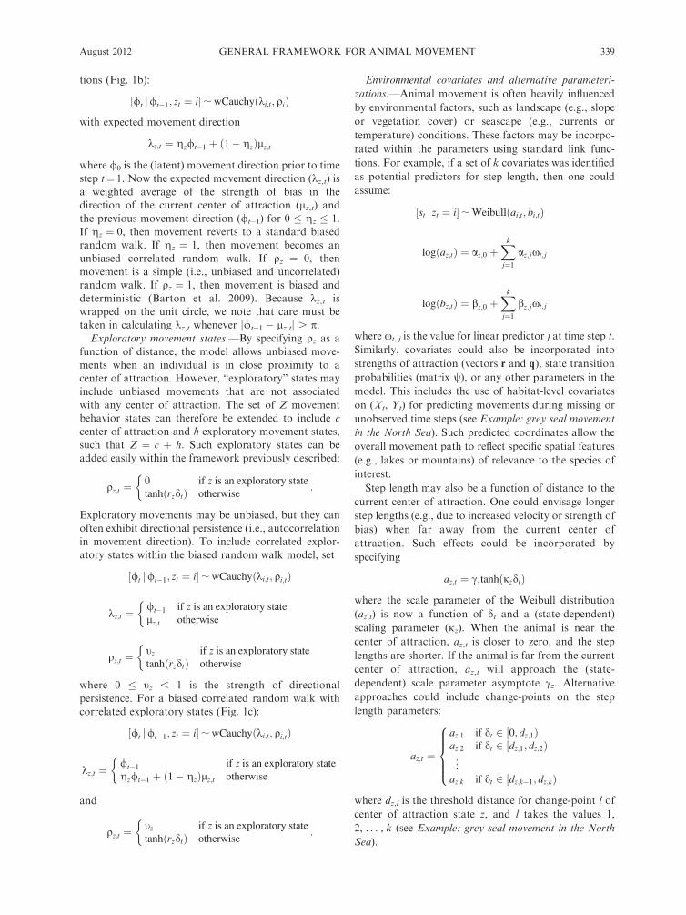
tions (Fig. 1b):

½/t j/t�1; zt ¼ i�; wCauchyðki;t; qiÞ

with expected movement direction

kz;t ¼ gz/t�1 þ ð1� gzÞlz;t

where /0 is the (latent) movement direction prior to time

step t¼ 1. Now the expected movement direction (kz,t) isa weighted average of the strength of bias in the

direction of the current center of attraction (lz,t) and

the previous movement direction (/t�1) for 0 � gz � 1.

If gz ¼ 0, then movement reverts to a standard biased

random walk. If gz ¼ 1, then movement becomes an

unbiased correlated random walk. If qz ¼ 0, then

movement is a simple (i.e., unbiased and uncorrelated)

random walk. If qz ¼ 1, then movement is biased and

deterministic (Barton et al. 2009). Because kz,t is

wrapped on the unit circle, we note that care must be

taken in calculating kz,t whenever j/t�1 � lz,tj . p.Exploratory movement states.—By specifying qz as a

function of distance, the model allows unbiased move-

ments when an individual is in close proximity to a

center of attraction. However, ‘‘exploratory’’ states may

include unbiased movements that are not associated

with any center of attraction. The set of Z movement

behavior states can therefore be extended to include c

center of attraction and h exploratory movement states,

such that Z ¼ c þ h. Such exploratory states can be

added easily within the framework previously described:

qz;t ¼0 if z is an exploratory state

tanhðrzdtÞ otherwise:

�

Exploratory movements may be unbiased, but they canoften exhibit directional persistence (i.e., autocorrelation

in movement direction). To include correlated explor-

atory states within the biased random walk model, set

½/t j/t�1; zt ¼ i�; wCauchyðki;t; qi;tÞ

kz;t ¼/t�1 if z is an exploratory state

lz;t otherwise

�

qz;t ¼tz if z is an exploratory state

tanhðrzdtÞ otherwise

�

where 0 � tz , 1 is the strength of directional

persistence. For a biased correlated random walk with

correlated exploratory states (Fig. 1c):


kz;t ¼/t�1 if z is an exploratory state

gz/t�1 þ ð1� gzÞlz;t otherwise

�

and

qz;t ¼tz if z is an exploratory state

tanhðrzdtÞ otherwise:

�

Environmental covariates and alternative parameteri-

zations.—Animal movement is often heavily influenced

by environmental factors, such as landscape (e.g., slope

or vegetation cover) or seascape (e.g., currents or

temperature) conditions. These factors may be incorpo-

rated within the parameters using standard link func-

tions. For example, if a set of k covariates was identified

as potential predictors for step length, then one could

assume:

½st j zt ¼ i�; Weibullðai;t; bi;tÞ

logðaz;tÞ ¼ az;0 þXk

j¼1

az;jxt;j

logðbz;tÞ ¼ bz;0 þXk

j¼1

bz;jxt;j

where xt, j is the value for linear predictor j at time step t.

Similarly, covariates could also be incorporated into

strengths of attraction (vectors r and q), state transition

probabilities (matrix w), or any other parameters in the

model. This includes the use of habitat-level covariates

on (Xt, Yt) for predicting movements during missing or

unobserved time steps (see Example: grey seal movement

in the North Sea). Such predicted coordinates allow the

overall movement path to reflect specific spatial features

(e.g., lakes or mountains) of relevance to the species of

interest.

Step length may also be a function of distance to the

current center of attraction. One could envisage longer

step lengths (e.g., due to increased velocity or strength of

bias) when far away from the current center of

attraction. Such effects could be incorporated by

specifying

az;t ¼ cztanhðjzdtÞ

where the scale parameter of the Weibull distribution

(az,t) is now a function of dt and a (state-dependent)

scaling parameter (jz). When the animal is near the

center of attraction, az,t is closer to zero, and the step

lengths are shorter. If the animal is far from the current

center of attraction, az,t will approach the (state-

dependent) scale parameter asymptote cz. Alternative

approaches could include change-points on the step

length parameters:

az;t ¼

az;1 if dt 2 ½0; dz;1Þaz;2 if dt 2 ½dz;1; dz;2Þ

..

.

az;k if dt 2 ½dz;k�1; dz;kÞ

8>>><>>>:

where dz,l is the threshold distance for change-point l of

center of attraction state z, and l takes the values 1,

2, . . . , k (see Example: grey seal movement in the North

Sea).


Much of the biological interest in multistate movement

models lies in the specification of behavioral state

transition probabilities. Depending on the biological

questions of interest, it may often be advantageous to

reparameterize the state transition probability matrix.

For example, with a migratory species it may be desirable

to restrict state transitions until the individual is in the

vicinity of the current center of attraction (i.e., so that ‘‘en

route’’ switches are avoided). A simple reparameteriza-

tion allows such behaviors to be more easily investigated:

w ¼

a1 ð1� a1Þb1;2 . . . ð1� a1Þb1;c

ð1� a2Þb2;1 a2 ð1� a2Þb2;c

..

. ... . .

. ...

ð1� acÞbc;1 ð1� acÞbc;2 . . . ac

26664

37775

where ai¼Pr(zt¼ i j zt�1¼ i), bk,i¼Pr(zt¼ i j zt�1¼ k, k 6¼i), and

Pci 6¼k bk;i ¼ 1 for k¼ 1, 2, . . . , c. Using logit-linear

intercept (fz) and slope (nz) parameters, state transitions

could incorporate the effects of distance:d

logitðaz;tÞ ¼ fz þ nzdt

whereby individuals could be more likely to remain in the

current movement state until they are in close proximity

to the associated center of attraction. More complicated

covariate structures (e.g., the amount of time in the

current state) or other reparameterizations could be

incorporated in a similar fashion.

STATE-SPACE FORMULATION

Even in well-designed studies, there typically will be

some degree of measurement error in spatiotemporal

animal location data. Environmental conditions may

affect the timing and location of fixes, as may animal

behavior (e.g., diving or burrowing species). For reliable

inference, these irregularities must be accounted for

when applying the mechanistic movement models just

described. To account for spatial error and temporal

irregularity, we propose a continuous-time observation

model to accompany our discrete-time movement

process model in a state-space formulation.

In the movement process model, we assume that

switches between behavioral states can occur at regular

time intervals of equal length. The switching interval

length must therefore be chosen at a temporal resolution

of relevance to the species and conditions of interest.

Similar to Jonsen et al. (2005), we assume that individuals

travel in a straight line between times t � 1 and t. The

observed locations are labeled according to the regular

time interval into which they fall: we write (xt,i, yt,i) for the

ith observation between time t� 1 and t, for i¼ 1, . . . , nt.These are related to the regular locations (Xt, Yt) via

xt;i ¼ ð1� jt;iÞXt�1 þ jt;iXt þ ext;i

yt;i ¼ ð1� jt;iÞYt�1 þ jt;iYt þ eyt;i

with the following error terms:

ext;i; Nð0;r2

xÞ

eyj;i; Nð0;r2

yÞ

where jt,i 2 [0, 1) is the proportion of the time interval

between locations (Xt�1, Yt�1) and (Xt, Yt) at which the

ith observation between times t� 1 and t was obtained.

Time intervals with no observations (i.e., nt¼ 0) do not

contribute to the observation model likelihood. In some

applications (e.g., radiotelemetry triangulation or Argos

satellite locations), the measurement errors are known to

have more frequent large outliers than would occur

under a normal distribution; in this case, a heavier-tailed

error distribution could be employed (e.g., t distribu-

tion) that allows additional noncentral or scale param-

eters (e.g., Jonsen et al. 2005).

EXAMPLE: GREY SEAL MOVEMENT IN THE NORTH SEA

Background

We demonstrate the application of our model using

hybrid-GPS transmitter data collected from grey seals

(Halichoerus grypus) in the North Sea. Fastloc GPS

transmitter (Wildtrack Telemetry Systems, Leeds, UK)

tags were deployed in April 2008 and attempted to

obtain a location every 30 minutes until battery failure

in August or September 2008. Our multistate random

walk model was initially deemed appropriate for grey

seals because we suspected that they could display

oriented movements among haul-out colonies and

foraging patches. However, a combination of biological

and technological issues necessitated use of the state-

space model previously described: (1) positions are only

attainable when an individual surfaces; hence, observa-

tions were obtained at irregular time intervals; and (2)

following any ‘‘dry’’ period where a transmitter

remained out of water for more than 10 minutes, no

new fixes could be obtained until the transmitter

returned to water continuously for 40 seconds. In other

words, there were frequent missing data due to an

inability to obtain locations while an individual was

either hauled out or underwater.

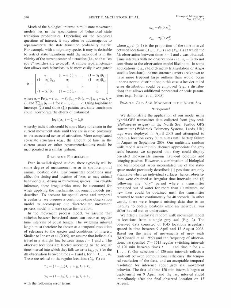
We fitted a multistate random walk movement model

to locations from a single grey seal (Fig. 2). The

observed data consisted of 1045 locations irregularly

spaced in time between 9 April and 13 August 2008.

Based on the scale of movements of grey seals

(McConnell et al. 1999) and the frequency of observa-

tions, we specified T ¼ 1515 regular switching intervals

of 120 min between times t � 1 and time t for t ¼1, . . . , T. Our selection of 120-min intervals reflects a

trade-off between computational efficiency, the tempo-

ral resolution of the data, and an acceptable temporal

resolution for inference about grey seal movement

behavior. The first of these 120-min intervals began at

deployment on 9 April, and the last interval ended

immediately after the final observed location on 13

August.


Movement model specification

For demonstrative purposes, we specify a simplified

model of grey seal movement by limiting the number of

centers of attraction (c ¼ 3) and exploratory states (h ¼2). Our most general first-order Markov movement

process model therefore consisted of Z ¼ 5 potential

states, including state dependence on both movement

direction and step length parameters:


kz;t ¼gz/t�1 þ ð1� gzÞlz;t if z � c/t�1 if z . c

�

qz;t ¼logit�1ðmz þ rzdt þ qzd

2t Þ if z � c

tz if z . c

�

½st j zt ¼ i�; Weibullðai;t; bi;tÞ

az;t ¼az;1½1� I½0;dzÞðdtÞ� þ az;2I½0;dzÞðdtÞ if z � caz if z . c

�

bz;t ¼bz;1½1� I½0;dzÞðdtÞ� þ bz;2I½0;dzÞðdtÞ if z � cbz if z . c

�

½zt j zt�1 ¼ k�; Categoricalðwk;1; :::;wk;5Þ

where k¼1, 2, 3, 4, 5; mz is an intercept term on the logit

scale; 0 � qz,t , 1; dt is the (scaled) Euclidean distance

between the predicted location (Xt�1, Yt�1) and center of

attraction (X*z , X*

z ) at time t; and I½0;dzÞðdtÞ is an indicator

function for dt 2 [0, dz). We chose to fit our state-space

model using Bayesiananalysis methods because of the

general complexity of the model and the ease by which

these methods can accommodate prior information,

latent state variables, and missing data (Ellison 2004,

King et al. 2009). Posterior model probabilities also

provide a straightforward means for addressing model

selection uncertainty (see Model selection and multi-

model inference).

For our Bayesian analysis, we specified uninformative

prior distributions for most of the parameters (Table 1).

Based on previous studies of grey seal movements

(McConnell et al. 1999), we specified a (conservative)

maximum sustainable speed of 2 m/s (such that st � 14.4

km). For the UTM coordinates of the centers of

attraction (X*z , Y*

z ), we specified joint discrete uniform

priors over the coordinates of the predicted locations

(Xt, Yt). This prior specification therefore assumes that

the centers of attraction are located on the predicted

movement path. We constrained state assignments for

time steps corresponding to (X*z , Y*

z ) for each center of

attraction, such that zt¼ k if (X*k , Y*

k )¼ (Xt, Yt) for k¼1, . . . , c. For the coordinates of the initial location (X0,

Y0), we specified a joint uniform prior over the region

(A) defined by the North Sea and coastline of Great

Britain. We also constrained predicted locations (Xt, Yt)

to be within A for t ¼ 1, . . . , T (i.e., inland grey seal

locations were prohibited a priori ).

Model selection and multi-model inference

We used a reversible-jump Markov chain Monte

Carlo (RJMCMC) algorithm (Green 1995) to fit the

model and simultaneously investigate various (state-

specific) parameterizations for the strength of bias

toward any centers of attraction and the correlations

between successive movements (see Appendix B). These

parameterizations included models with linear bias [qz,t¼ logit�1(mzþ rzdt)] and quadratic bias [qz,t¼ logit�1(mz

þ rzdtþ qzd2t )] toward centers of attraction for z¼ 1, 2, 3.

We also investigated models with no correlation in

movement direction between successive time steps when

FIG. 2. Observed locations for a grey seal (Halichoerus grypus) as it traveled clockwise among a foraging area in the North Seaand haul-out sites on the eastern coast of Great Britain.


in a center of attraction state (gz¼0 for z¼1, 2, 3) or an

exploratory state (tz ¼ 0 for z ¼ 4, 5).

These different parameterizations yielded 256 poten-

tial models for evaluation via posterior model probabil-

ities. For all models, we assumed equal prior model

probabilities. For all parameters without standard full

conditional posterior distributions, random walk Me-

tropolis-Hastings updates were used (e.g., Brooks 1998,

Givens and Hoeting 2005). After initial pilot tuning and

burn-in, we produced a single MCMC chain of five

million iterations for calculating posterior summaries

and model probabilities. After thinning by 100 iterations

to reduce memory requirements, Monte Carlo estimates

(including model-averaged estimates) were obtained for

each of the parameters from this single Markov chain.

The RJMCMC algorithm was written in the C

programming language (Kernighan and Ritchie 1988),

with pre- and post-processing performed in R via the .C

Interface (R Development Core Team 2009).

Example results and discussion

Posterior model probabilities (Table 2) and model-

averaged parameter summaries (Table 3) indicate biased

movements toward all three centers of attraction. The

estimated coordinates of the centers of attraction

correspond to the Farne Islands haul-out site, the

Abertay haul-out site, and the Dogger Bank foraging

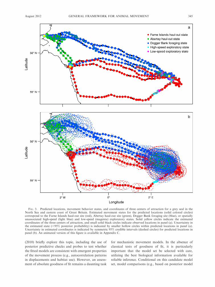
site (Fig. 3; Appendix C), and the strengths of bias to

these three sites differed as a function of distance (Fig.

4). The Abertay haul-out site maintained a strong and

consistent bias up to 350 km. Both the Farne Islands

haul-out and Dogger Bank foraging sites exhibited a

decreasing strength of bias curve, but we found little

evidence of a quadratic effect of distance (Tables 2 and

3). Biased movements continued at greater distances

(.350 km) and declined less rapidly from the Dogger

Bank foraging site than from the Farne Islands haul-out

site. These patterns of directed movement as a function

of distance could be indicative of the seal ‘‘honing in’’ on

these targets, but ocean currents are also likely to be

influencing the timing and direction of these movements

(see Gaspar et al. 2006).

Model-averaged posterior summaries indicated a

strong tendency for the seal to remain in its current

movement state (Table 3), with switches between center

of attraction states rarely occurring until the seal had

reached the vicinity of the current center of attraction

(Fig. 3). We found very little evidence of correlated

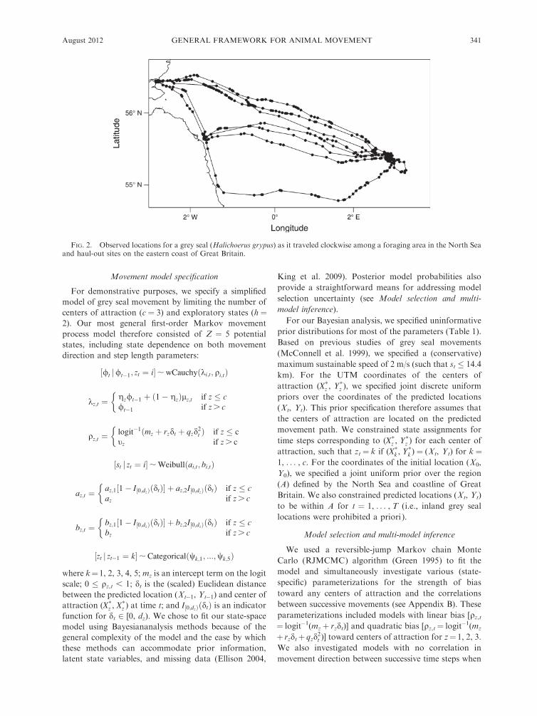
TABLE 1. Parameter definitions and (uninformative) prior specifications for a Bayesian analysis of grey seal (Halichoerus grypus)location data using the multistate random walk movement model.

Parameter Description Prior distribution

mz Intercept term for the strength of bias as a function of distance to center ofattraction, z ¼ 1, 2, 3.

Nð0; s2Þ

rz Linear term for the strength of bias as a function of distance to center of attraction, z¼ 1, 2, 3.

Nð0; s2Þ

qz Quadratic term for the strength of bias as a function of distance to center ofattraction, z ¼ 1, 2, 3.

Nð0; s2Þ

s2 Prior variance for mz; rz; and qz. C�1ð3; 2Þgz Movement direction correlation term for center of attraction, z ¼ 1, 2, 3. Unifð0; 1Þtz Movement direction correlation term for exploratory state, z ¼ 4, 5. Unifð0; 1Þ/0 Direction (or bearing) of movement for initial time step, t ¼ 0. Unifð0; 2pÞaz Scale parameter (meters) of the Weibull distribution for step length of states, z ¼

1, 2, 3, 4, 5.Unifð0; 14 400Þ

bz Shape parameter of the Weibull distribution for step length of states, z ¼ 1, 2, 3, 4, 5. Unifð0; 30Þdz Change-point distance (meters) for scale and shape parameters of the Weibull

distribution for step length of center of attraction states, z ¼ 1, 2, 3.Unifð0; 400 000Þ

r2x Measurement error variance for easting coordinates of observed locations ðxt;i; yt;iÞ. C�1ð10�3; 10�3Þ

r2y Measurement error variance for northing coordinates of observed locations ðxt;i; yt;iÞ. C�1ð10�3; 10�3Þ

w½k;�� The kth row vector of the state transition probability matrix, with each element ðwk;iÞcorresponding to the switching probability from state k at time t � 1 to state i ¼1, 2, 3, 4, 5 at time t.

Dirichletð1; 1; 1; 1; 1Þ

TABLE 2. Posterior model probabilities (PMP) for strength ofattraction (qz) and correlation (gz and tz) parameters for agrey seal in the North Sea.

PMP

Model parameter

q1 q2 q3 g1 g2 g3 t4 t5

0.17 10.15 1 10.13 1 10.11 1 1 10.070.07 10.06 10.05 1 10.03 1 10.03 1 1 10.02 1 1 10.02 1 1 1 1MPP 0.43 0.68 0.48 0.01 0.00 0.00 0.16 0.01

Notes: For each parameter, ‘‘1’’ indicates presence in themodel. The bottom row indicates the marginal posteriorprobabilities (MPP) for each parameter. Centers of attraction(denoted by variable subscript numbers) correspond to theFarne Islands haul-out site (z¼1), Abertay haul-out site (z¼2),and Dogger Bank foraging site (z¼ 3). Other states correspondto high-speed (z ¼ 4) and low-speed (z ¼ 5) exploratory states.Results are for models with a PMP of at least 0.02.


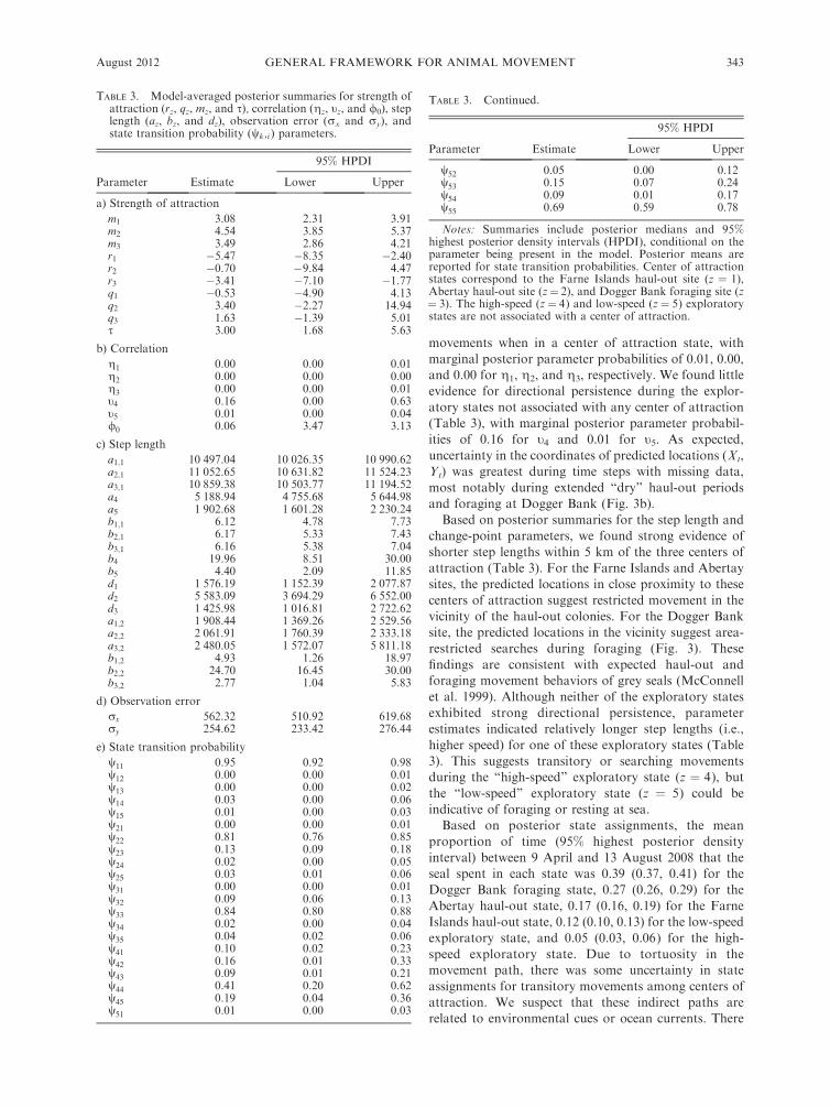
movements when in a center of attraction state, with

marginal posterior parameter probabilities of 0.01, 0.00,and 0.00 for g1, g2, and g3, respectively. We found little

evidence for directional persistence during the explor-

atory states not associated with any center of attraction(Table 3), with marginal posterior parameter probabil-

ities of 0.16 for t4 and 0.01 for t5. As expected,

uncertainty in the coordinates of predicted locations (Xt,Yt) was greatest during time steps with missing data,

most notably during extended ‘‘dry’’ haul-out periods

and foraging at Dogger Bank (Fig. 3b).

Based on posterior summaries for the step length andchange-point parameters, we found strong evidence of

shorter step lengths within 5 km of the three centers of

attraction (Table 3). For the Farne Islands and Abertaysites, the predicted locations in close proximity to these

centers of attraction suggest restricted movement in the

vicinity of the haul-out colonies. For the Dogger Banksite, the predicted locations in the vicinity suggest area-

restricted searches during foraging (Fig. 3). These

findings are consistent with expected haul-out andforaging movement behaviors of grey seals (McConnell

et al. 1999). Although neither of the exploratory states

exhibited strong directional persistence, parameterestimates indicated relatively longer step lengths (i.e.,

higher speed) for one of these exploratory states (Table

3). This suggests transitory or searching movementsduring the ‘‘high-speed’’ exploratory state (z ¼ 4), but

the ‘‘low-speed’’ exploratory state (z ¼ 5) could be

indicative of foraging or resting at sea.Based on posterior state assignments, the mean

proportion of time (95% highest posterior density

interval) between 9 April and 13 August 2008 that theseal spent in each state was 0.39 (0.37, 0.41) for the

Dogger Bank foraging state, 0.27 (0.26, 0.29) for the

Abertay haul-out state, 0.17 (0.16, 0.19) for the FarneIslands haul-out state, 0.12 (0.10, 0.13) for the low-speed

exploratory state, and 0.05 (0.03, 0.06) for the high-

speed exploratory state. Due to tortuosity in themovement path, there was some uncertainty in state

assignments for transitory movements among centers of

attraction. We suspect that these indirect paths arerelated to environmental cues or ocean currents. There

TABLE 3. Model-averaged posterior summaries for strength ofattraction (rz, qz, mz, and s), correlation (gz, tz, and /0), steplength (az, bz, and dz), observation error (rx and ry), andstate transition probability (wk,i ) parameters.

Parameter Estimate

95% HPDI

Lower Upper

a) Strength of attraction

m1 3.08 2.31 3.91m2 4.54 3.85 5.37m3 3.49 2.86 4.21r1 �5.47 �8.35 �2.40r2 �0.70 �9.84 4.47r3 �3.41 �7.10 �1.77q1 �0.53 �4.90 4.13q2 3.40 �2.27 14.94q3 1.63 �1.39 5.01s 3.00 1.68 5.63

b) Correlation

g1 0.00 0.00 0.01g2 0.00 0.00 0.00g3 0.00 0.00 0.01t4 0.16 0.00 0.63t5 0.01 0.00 0.04/0 0.06 3.47 3.13

c) Step length

a1;1 10 497.04 10 026.35 10 990.62a2;1 11 052.65 10 631.82 11 524.23a3;1 10 859.38 10 503.77 11 194.52a4 5 188.94 4 755.68 5 644.98a5 1 902.68 1 601.28 2 230.24b1;1 6.12 4.78 7.73b2;1 6.17 5.33 7.43b3;1 6.16 5.38 7.04b4 19.96 8.51 30.00b5 4.40 2.09 11.85d1 1 576.19 1 152.39 2 077.87d2 5 583.09 3 694.29 6 552.00d3 1 425.98 1 016.81 2 722.62a1;2 1 908.44 1 369.26 2 529.56a2;2 2 061.91 1 760.39 2 333.18a3;2 2 480.05 1 572.07 5 811.18b1;2 4.93 1.26 18.97b2;2 24.70 16.45 30.00b3;2 2.77 1.04 5.83

d) Observation error

rx 562.32 510.92 619.68ry 254.62 233.42 276.44

e) State transition probability

w11 0.95 0.92 0.98w12 0.00 0.00 0.01w13 0.00 0.00 0.02w14 0.03 0.00 0.06w15 0.01 0.00 0.03w21 0.00 0.00 0.01w22 0.81 0.76 0.85w23 0.13 0.09 0.18w24 0.02 0.00 0.05w25 0.03 0.01 0.06w31 0.00 0.00 0.01w32 0.09 0.06 0.13w33 0.84 0.80 0.88w34 0.02 0.00 0.04w35 0.04 0.02 0.06w41 0.10 0.02 0.23w42 0.16 0.01 0.33w43 0.09 0.01 0.21w44 0.41 0.20 0.62w45 0.19 0.04 0.36w51 0.01 0.00 0.03

TABLE 3. Continued.

Parameter Estimate

95% HPDI

Lower Upper

w52 0.05 0.00 0.12w53 0.15 0.07 0.24w54 0.09 0.01 0.17w55 0.69 0.59 0.78

Notes: Summaries include posterior medians and 95%highest posterior density intervals (HPDI), conditional on theparameter being present in the model. Posterior means arereported for state transition probabilities. Center of attractionstates correspond to the Farne Islands haul-out site (z ¼ 1),Abertay haul-out site (z¼ 2), and Dogger Bank foraging site (z¼ 3). The high-speed (z¼ 4) and low-speed (z¼ 5) exploratorystates are not associated with a center of attraction.


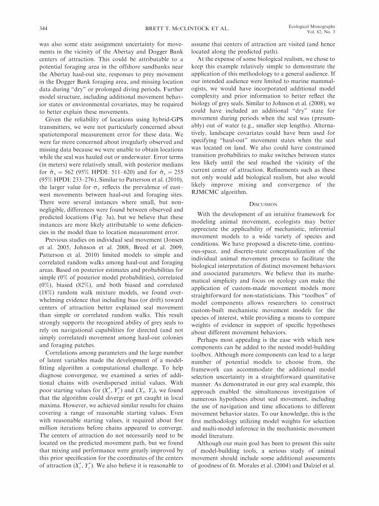
was also some state assignment uncertainty for move-

ments in the vicinity of the Abertay and Dogger Bank

centers of attraction. This could be attributable to a

potential foraging area in the offshore sandbanks near

the Abertay haul-out site, responses to prey movement

in the Dogger Bank foraging area, and missing location

data during ‘‘dry’’ or prolonged diving periods. Further

model structure, including additional movement behav-

ior states or environmental covariates, may be required

to better explain these movements.

Given the reliability of locations using hybrid-GPS

transmitters, we were not particularly concerned about

spatiotemporal measurement error for these data. We

were far more concerned about irregularly observed and

missing data because we were unable to obtain locations

while the seal was hauled out or underwater. Error terms

(in meters) were relatively small, with posterior medians

for rx ¼ 562 (95% HPDI: 511–620) and for ry ¼ 255

(95% HPDI: 233–276). Similar to Patterson et al. (2010),

the larger value for rx reflects the prevalence of east–

west movements between haul-out and foraging sites.

There were several instances where small, but non-

negligible, differences were found between observed and

predicted locations (Fig. 3a), but we believe that these

instances are more likely attributable to some deficien-

cies in the model than to location measurement error.

Previous studies on individual seal movement (Jonsen

et al. 2005, Johnson et al. 2008, Breed et al. 2009,

Patterson et al. 2010) limited models to simple and

correlated random walks among haul-out and foraging

areas. Based on posterior estimates and probabilities for

simple (0% of posterior model probabilities), correlated

(0%), biased (82%), and both biased and correlated

(18%) random walk mixture models, we found over-

whelming evidence that including bias (or drift) toward

centers of attraction better explained seal movement

than simple or correlated random walks. This result

strongly supports the recognized ability of grey seals to

rely on navigational capabilities for directed (and not

simply correlated) movement among haul-out colonies

and foraging patches.

Correlations among parameters and the large number

of latent variables made the development of a model-

fitting algorithm a computational challenge. To help

diagnose convergence, we examined a series of addi-

tional chains with overdispersed initial values. With

poor starting values for (X*z , Y*

z ) and (Xt, Yt), we found

that the algorithm could diverge or get caught in local

maxima. However, we achieved similar results for chains

covering a range of reasonable starting values. Even

with reasonable starting values, it required about five

million iterations before chains appeared to converge.

The centers of attraction do not necessarily need to be

located on the predicted movement path, but we found

that mixing and performance were greatly improved by

this prior specification for the coordinates of the centers

of attraction (X*z , Y*

z ). We also believe it is reasonable to

assume that centers of attraction are visited (and hence

located along the predicted path).

At the expense of some biological realism, we chose to

keep this example relatively simple to demonstrate the

application of this methodology to a general audience. If

our intended audience were limited to marine mammal-

ogists, we would have incorporated additional model

complexity and prior information to better reflect the

biology of grey seals. Similar to Johnson et al. (2008), we

could have included an additional ‘‘dry’’ state for

movement during periods when the seal was (presum-

ably) out of water (e.g., smaller step lengths). Alterna-

tively, landscape covariates could have been used for

specifying ‘‘haul-out’’ movement states when the seal

was located on land. We also could have constrained

transition probabilities to make switches between states

less likely until the seal reached the vicinity of the

current center of attraction. Refinements such as these

not only would add biological realism, but also would

likely improve mixing and convergence of the

RJMCMC algorithm.

DISCUSSION

With the development of an intuitive framework for

modeling animal movement, ecologists may better

appreciate the applicability of mechanistic, inferential

movement models to a wide variety of species and

conditions. We have proposed a discrete-time, continu-

ous-space, and discrete-state conceptualization of the

individual animal movement process to facilitate the

biological interpretation of distinct movement behaviors

and associated parameters. We believe that its mathe-

matical simplicity and focus on ecology can make the

application of custom-made movement models more

straightforward for non-statisticians. This ‘‘toolbox’’ of

model components allows researchers to construct

custom-built mechanistic movement models for the

species of interest, while providing a means to compare

weights of evidence in support of specific hypotheses

about different movement behaviors.

Perhaps most appealing is the ease with which new

components can be added to the nested model-building

toolbox. Although more components can lead to a large

number of potential models to choose from, the

framework can accommodate the additional model

selection uncertainty in a straightforward quantitative

manner. As demonstrated in our grey seal example, this

approach enabled the simultaneous investigation of

numerous hypotheses about seal movement, including

the use of navigation and time allocations to different

movement behavior states. To our knowledge, this is the

first methodology utilizing model weights for selection

and multi-model inference in the mechanistic movement

model literature.

Although our main goal has been to present this suite

of model-building tools, a serious study of animal

movement should include some additional assessments

of goodness of fit. Morales et al. (2004) and Dalziel et al.


(2010) briefly explore this topic, including the use of

posterior predictive checks and probes to test whether

the fitted models are consistent with emergent properties

of the movement process (e.g., autocorrelation patterns

in displacements and habitat use). However, an assess-

ment of absolute goodness of fit remains a daunting task

for mechanistic movement models. In the absence of

classical tests of goodness of fit, it is particularly

important that the model set be selected with care,

utilizing the best biological information available for

reliable inference. Conditional on this candidate model

set, model comparisons (e.g., based on posterior model

FIG. 3. Predicted locations, movement behavior states, and coordinates of three centers of attraction for a grey seal in theNorth Sea and eastern coast of Great Britain. Estimated movement states for the predicted locations (solid colored circles)correspond to the Farne Islands haul-out site (red), Abertay haul-out site (green), Dogger Bank foraging site (blue), or spatiallyunassociated high-speed (light blue) and low-speed (magenta) exploratory states. Solid yellow circles indicate the estimatedcoordinates of the three centers of attraction, and small solid black circles indicate observed locations in panel (a). Uncertainty inthe estimated state (,95% posterior probability) is indicated by smaller hollow circles within predicted locations in panel (a).Uncertainty in estimated coordinates is indicated by symmetric 95% credible intervals (dashed circles) for predicted locations inpanel (b). An animated version of this figure is available in Appendix C.


probabilities or other model selection criteria) can

provide some assessment of the relative goodness of fit.

There remain many potential extensions to the

modeling framework beyond those already identified.

In the grey seal example, we included two exploratory

movement states not associated with any center of

attraction, but additional spatially unassociated states

that differ in their movement properties (and associated

state parameters) may be incorporated (sensu Morales et

al. 2004, Jonsen et al. 2005, Breed et al. 2009). These

additional states could be used to further differentiate

among exploratory movements (e.g., dispersal or search

strategies) that have unique distributions for step length

and the degree of correlation between successive

movements.

We reiterate that centers of attraction do not

necessarily refer to a single location in space. Rather,

they can refer to any entity to which animals move in

response. This includes immobile entities such as habitat

patches, but also mobile entities such as conspecifics or

prey. Any given entity (or group of entities) could

therefore be used to define a different behavior state for

movement toward, away from, or within each entity.

Potential centers of attraction also can be dynamically

incorporated within an individual’s portfolio as its

habitat is explored, thus allowing for explicit modeling

of the effects of past experience on movement. Instead of

centers of attraction, centers of repulsion (where�1 , qz� 0) may be particularly useful for demonstrating

avoidance behaviors related to encounters with conspe-

cifics, predators, or undesirable habitats.

From a behavioral ecology perspective, perhaps most

promising is the potential for modeling movement state

transition probabilities. By incorporating physiological

or environmental covariate information into the frame-

work, one can investigate hypotheses about the timing

and motivations behind various movement behaviors as

individuals respond to changes in the internal and

external environment (Morales et al. 2010). Biotelemetry

data (e.g., metabolic rate) or time of year (e.g., breeding

season) are among many factors that may help to

explain changes in movement behavior. Instead of

relying solely on trajectories, ancillary data may also

be helpful in the assignment of movement states. For

example, additional landscape or seascape information

may have better explained the indirect movements

between the two haul-out colonies in our grey seal

analysis. Recent advances, such as animal-borne accel-

erometers (Wilson et al. 2008, Holland et al. 2009, Payne

et al. 2011), will probably provide additional ways to

distinguish among different types of movement (e.g.,

predator hunting and feeding). There are also many

ways by which memory can be incorporated into

movements and state transitions. Here, we only explored

two such mechanisms for memory, including Markov

processes for state transitions and the existence of

spatial locations that are committed to memory because

they are (presumably) associated with specific goals.

The locations of centers of attraction are typically

assumed to be known based on prior knowledge or

qualitative assessments of the data. Indeed, one could

relatively easily predict the coordinates of the three

centers of attraction in our grey seal example using only

the naked eye or previous studies. However, we envision

more complicated movement paths where it is very

difficult to identify or differentiate between potential

FIG. 4. Model-averaged strength of bias (qz) to three centers of attraction as a function of distance from a grey seal in the NorthSea. Center of attraction states correspond to the Farne Islands haul-out site, Abertay haul-out site, and Dogger Bank foraging site.Thinner lines indicate symmetric 95% credible intervals. Lines terminate at the maximum distance at which the seal was assigned toeach respective center of attraction state.


centers. We believe that a quantitative means for

estimating the location of centers and their associated

strengths of attraction (or repulsion), such as that

proposed here, improves our ability to extract reliable

information from novel or more complex movement

paths.

For simplicity, we chose to specify three centers of

attraction in our grey seal example. Although we found

strong evidence of bias toward all three of these centers,

if any center z receives little support for bias (e.g., qz,t ’

0 for all dt), alternative models removing such centers

should be explored because state z essentially becomes

an uncorrelated exploratory state. This may have

undesirable consequences, including confounded explor-

atory states and poor MCMC mixing. Ideally, the model

could be extended to accommodate an unknown

number of centers and reduce any need for ad hoc

assessments of the appropriate number of centers. This

would require an additional parameter for the number

of centers and (state-specific) movement parameters for

each potential center. Similar to the multi-model

inference procedure used here, a reversible-jump

MCMC algorithm could be utilized to estimate the

number of centers of attraction. This potential extension

constitutes the focus of current research.

Additional information or structural complexity

could also be specified in the observation process of

the state-space model. For example, Jonsen et al. (2005)

specified informative priors for measurement error

parameters based on previously published records of

location estimation error for Argos-tagged grey seals.

State-dependent error or correlation terms (e.g., utilizing

a multivariate normal error distribution) could also be

incorporated. Although a great deal of previous effort in

the analysis of animal location data has focused on the

observation process, we expect greater emphasis on the

movement process as the quality of location data

continues to improve (e.g., with advances in GPS

technology).

Although other approaches (e.g., Blackwell 2003,

Jonsen et al. 2005, Johnson et al. 2008) potentially could

be extended to include the various types of movement

accommodated by our multistate model, we chose to

extend the basic methodology of Morales et al. (2004)

because of its intuitive appeal to ecologists and wildlife

professionals. The discrete-time, continuous-space ap-

proach of Jonsen et al. (2005) can accommodate

correlated and uncorrelated exploratory movements,

but it does not include biased or area-restricted

movements related to specific locations or habitats. An

additional limitation of the correlated random walk

approach of Jonsen et al. (2005) is a lack of indepen-

dence between direction and step length, resulting in

higher-order autocorrelations than found in standard

correlated random walks. Our approach assumes

independence between direction and step length for

each movement behavior state, but a joint distribution

including correlations could potentially be incorporated

if deemed appropriate (e.g., specifying shorter step

lengths when movement is away from the current center

of attraction).

The continuous-time, continuous-space approaches of

Blackwell (2003) and Johnson et al. (2008) do allow

correlated movements and ‘‘drift’’ that can (potentially)

be related to specific locations (sensu Kendall 1974,

Dunn and Gipson 1977). However, Blackwell (2003)

assumes that movement behavior states are known and

Johnson et al. (2008) only include a single state with

known covariates; hence, neither approach includes an

estimation framework for both movement state and

switching behavior. Although satisfying from a mathe-

matical and theoretical perspective, we believe the often

difficult interpretation of continuous-time movement

parameters (e.g., those related to Ornstein-Uhlenbeck

and other diffusion processes) can, in practice, be

discouraging to applied ecologists wishing to use or

extend these methods. This may change as ecologists

become more familiar with the principles of mechanistic

movement models and computer software makes these

approaches more accessible.

Unlike continuous-time movement process models,

the primary disadvantage of a discrete-time approach is

that the time scale between state transitions must be

chosen based on the biology of the species and the

frequency of observations. For any continuous- or

discrete-time approach to be useful, the temporal

resolution of the observed data must be relevant to the

specific movement behaviors of interest. The timing and

frequency of observations must therefore be carefully

considered when designing telemetry devices and data

collection schemes.

To encourage the broader application of movement

models in ecology, user-friendly software for the analysis

of animal location data is needed. Ovaskainen et al.

(2008) and Johnson et al. (2008) provided important first

steps in accessible software by creating DISPERSE and

the R package CRAWL to perform the complicated

computations that the models, respectively, require.

Despite its relative mathematical simplicity, the large

number of parameters and latent variables inherent to

our modeling framework also make implementation a

computational challenge. We therefore provide code for

the full state-space formulation of our model (see

Supplement) and are currently developing a software

package for general use by practitioners (L. Milazzo,

B. T. McClintock, R. King, L. Thomas, J. Matthiopou-

los, and J. M. Morales, unpublished software).

By making individual movement models more acces-

sible and readily interpretable to ecologists, we ulti-

mately hope that progress can be made toward linking

animal movement and population dynamics at the

interface of behavioral, population, and landscape

ecology (Morales et al. 2010). Although the mechanistic

links between animal movement and population dy-

namics are theoretically understood, fitting population-

level models to data from many individuals will pose


considerable mathematical and computational challeng-

es. Scaling individual movement models up to popula-

tion-level processes therefore remains a very promising

avenue for future research.

ACKNOWLEDGMENTS

Funding for this research was provided by the Engineeringand Physical Sciences Research Council (EPSRC reference EP/F069766/1). Hawthorne Beyer, Roland Langrock, TiagoMarques, Lorenzo Milazzo, and two anonymous refereesprovided helpful comments on the manuscript.

LITERATURE CITED

Anderson-Sprecher, R., and J. Ledolter. 1991. State-spaceanalysis of wildlife telemetry data. Journal of the AmericanStatistical Association 86:596–602.

Barton, K. A., B. L. Phillips, J. M. Morales, and J. M. J. Travis.2009. The evolution of an ‘‘intelligent’’ dispersal strategy:biased, correlated random walks in patchy landscapes. Oikos118:309–319.

Blackwell, P. G. 1997. Random diffusion models for animalmovement. Ecological Modelling 100:87–102.

Blackwell, P. G. 2003. Bayesian inference for Markov processeswith diffusion and discrete components. Biometrika 90:613–627.

Borchers, D. L., S. T. Buckland, and W. Zucchini. 2002.Estimating animal abundance: closed populations. Springer-Verlag, London, UK.

Breed, G. A., I. D. Jonsen, R. A. Myers, W. D. Bowen, andM. L. Leonard. 2009. Sex-specific, seasonal foraging tacticsof adult grey seals (Halichoerus grypus) revealed by state-space analysis. Ecology 90:3209–3221.

Brooks, S. P. 1998. Markov chain Monte Carlo and itsapplications. Statistician 47:69–100.

Brownie, C., J. E. Hines, J. D. Nichols, K. H. Pollock, and J. B.Hestbeck. 1993. Capture–recapture studies for multiple strataincluding non-Markovian transitions. Biometrics 49:1173–1187.

Buckland, S. T., D. R. Anderson, K. P. Burnham, J. L. Laake,D. L. Borchers, and L. Thomas. 2001. Introduction todistance sampling: estimating abundance of biologicalpopulations. Oxford University Press, New York, NewYork, USA.

Burnham, K. P., and D. R. Anderson. 2002. Model selectionand multi-model inference: a practical information-theoreticapproach. Second edition. Springer-Verlag, New York, NewYork, USA.

Cagnacci, F., L. Boitani, R. A. Powell, and M. S. Boyce. 2010.Animal ecology meets GPS-based radiotelemetry: a perfectstorm of opportunities and challenges. Philosophical Trans-actions of the Royal Society B 27:2157–2162.

Codling, E. A., R. N. Bearon, and G. J. Thorn. 2010. Diffusionabout the mean drift location in a biased random walk.Ecology 91:3106–3113.

Cooke, S. J., S. G. Hinch, M. Wikelski, R. D. Andrews, L. J.Kuchel, T. G. Wolcott, and P. J. Butler. 2004. Biotelemetry: amechanistic approach to ecology. Trends in Ecology andEvolution 19:334–343.

Dalziel, B. D., J. M. Morales, and J. M. Fryxell. 2010. Fittingdynamic models to animal movement data: the importance ofprobes for model selection, a reply to Franz and Caillaud.American Naturalist 175:762–764.

Dunn, J. E., and P. S. Gipson. 1977. Analysis of radio telemetrydata in studies of home range. Biometrics 33:85–101.

Dupuis, J. A. 1995. Bayesian estimation of movement andsurvival probabilities from capture–recapture data. Bio-metrika 82:761–772.

Ellison, A. M. 2004. Bayesian inference in ecology. EcologyLetters 7:509–520.

Forester, J. D., A. R. Ives, M. G. Turner, D. P. Anderson, D.Fortin, H. L. Beyer, D. W. Smith, and M. S. Boyce. 2007.State-space models link elk movement patterns to landscapecharacteristics in Yellowstone National Park. EcologicalMonographs 77:285–299.

Gao, J. 2002. Integration of GPS with remote sensing and GIS:reality and prospect. Photogrammetric Engineering andRemote Sensing 68:447–453.

Gaspar, P., J.-Y. Georges, S. Fossette, A. Lenoble, S. Ferraroli,and Y. Le Maho. 2006. Marine animal behaviour: neglectingocean currents can lead us up the wrong track. Proceedingsof the Royal Society B 273:2697–2702.

Givens, G. H., and J. A. Hoeting. 2005. Computationalstatistics. John Wiley, New York, New York, USA.

Green, P. J. 1995. Reversible jump Markov chain Monte Carlocomputation and Bayesian model determination. Biometrika82:711–732.

Hoeting, J. A., D. Madigan, A. E. Raftery, and C. T. Volinsky.1999. Bayesian model averaging: a tutorial. Statistical Science14:382–401.

Holland, R. A., M. Wikelski, F. Kummeth, and C. Bosque.2009. The secret life of oilbirds: new insights into themovement ecology of a unique avian frugivore. PLoS ONE4(12):e8264.

Holyoak, M., R. Casagrandi, R. Nathan, E. Revilla, and O.Spiegel. 2008. Trends and missing parts in the study ofmovement ecology. Proceedings of the National Academy ofSciences USA 105:10960–19065.

Johnson, D. S., J. M. London, M.-A. Lea, and J. W. Durban.2008. Continuous-time correlated random walk model foranimal telemetry data. Ecology 89:1208–1215.

Jonsen, I. D., J. M. Flemming, and R. A. Myers. 2005. Robuststate-space modeling of animal movement data. Ecology86:2874–2880.

Jonsen, I. D., R. A. Myers, and M. C. James. 2006. Robusthierarchical state-space models reveal diel variation in travelrates of migrating leatherback turtles. Journal of AnimalEcology 75:1046–1057.

Kendall, D. G. 1974. Pole-seeking Brownian motion and birdnavigation. Journal of the Royal Statistical Society B 36:365–417.

Kernighan, B. W., and D. M. Ritchie. 1988. The Cprogramming language. Second edition. Prentice Hall,Englewood Cliffs, New Jersey, USA.

King, R., and S. P. Brooks. 2002. Bayesian model discrimina-tion for multiple strata capture–recapture data. Biometrika89:785–806.

King, R., and S. P. Brooks. 2004. A classical study of catch-effort models for Hector’s dolphins. Journal of the AmericanStatistical Association 99:325–333.

King, R., B. J. T. Morgan, O. Gimenez, and S. P. Brooks. 2009.Bayesian analysis for population ecology. Chapman andHall/CRC, Boca Raton, Florida, USA.

Langrock, R., R. King, J. Matthiopoulos, L. Thomas, D.Fortin, and J. M. Morales. 2012. Flexible and practicalmodeling of animal telemetry data: hidden Markov modelsand extensions. Technical Report. University of St Andrews,St. Andrews, Scotland, UK.

MacKenzie, D. I., J. D. Nichols, J. A. Royle, K. H. Pollock,L. L. Bailey, and J. E. Hines. 2006. Occupancy estimationand modeling: inferring patterns and dynamics of speciesoccurrence. Elsevier, San Diego, California, USA.

McConnell, B. J., M. A. Fedak, S. K. Hooker, and T. A.Patterson. 2010. Telemetry. Pages 222–262 in I. L. Boyd,W. D. Bowen, and S. J. Iverson, editors. Marine mammalecology and conservation. Oxford University Press, Oxford,UK.

McConnell, B. J., M. A. Fedak, P. Lovell, and P. S. Hammond.1999. Movements and foraging areas of grey seals in theNorth Sea. Journal of Applied Ecology 36:573–590.


Morales, J. M., D. T. Haydon, J. Frair, K. E. Holsinger, andJ. M. Fryxell. 2004. Extracting more out of relocation data:building movement models as mixtures of random walks.Ecology 85:2436–2445.

Morales, J. M., P. R. Moorcroft, J. Matthiopoulos, J. L. Frair,J. G. Kie, R. A. Powell, E. H. Merrill, and D. T. Haydon.2010. Building the bridge between animal movement andpopulation dynamics. Philosophical Transactions of theRoyal Society B 365:2289–2301.

Otis, D. L., K. P. Burnham, G. C. White, and D. R. Anderson.1978. Statistical inference from capture data on closed animalpopulations. Wildlife Monographs 62:3–135.

Ovaskainen, O., H. Rekola, E. Meyke, and E. Arjas. 2008.Bayesian methods for analyzing movements in heterogeneouslandscapes from mark–recapture data. Ecology 89:542–554.

Patterson, T. A., B. J. McConnell, M. A. Fedak, M. V.Bravington, and M. A. Hindell. 2010. Using GPS data toevaluate the accuracy of state-space methods for correctionof Argos satellite telemetry error. Ecology 91:273–285.

Patterson, T. A., L. Thomas, C. Wilcox, O. Ovaskainen, and J.Matthiopoulos. 2008. State-space models of individualanimal movement. Trends in Ecology and Evolution 23:87–94.

Payne, N. L., B. M. Gillanders, R. S. Seymour, D. M. Webber,E. P. Snelling, and J. M. Semmens. 2011. Accelerometryestimates field metabolic rate in giant Australian cuttlefishSepia apama during breeding. Journal of Animal Ecology80:422–430.

R Development Core Team. 2009. R: A language andenvironment for statistical computing. R Foundation forStatistical Computing, Vienna, Austria. http://www.R-project.org

Schick, R. S., S. R. Loarie, F. Colchero, B. D. Best, A.Boustany, D. A. Conde, P. N. Halpin, L. N. Joppa, C. M.McClellan, and J. S. Clark. 2008. Understanding movement

data and movement processes: current and emergingdirections. Ecology Letters 11:1338–1350.

Schwarz, C. J. 2009. Migration and movement—the next stage.Pages 323–348 in D. L. Thomson, E. G. Cooch, and M. J.Conroy, editors. Modeling demographic processes in markedpopulations. Springer, New York, New York, USA.

Schwarz, C. J., J. F. Schweigert, and A. N. Arnason. 1993.Estimating migration rates using tag-recovery data. Biomet-rics 49:177–193.

Thomas, L., S. T. Buckland, E. A. Rexstad, J. L. Laake, S.Strindberg, S. L. Hedley, J. R. B. Bishop, T. A. Marques, andK. P. Burnham. 2010. Distance software: design and analysisof distance sampling surveys for estimating population size.Journal of Applied Ecology 47:5–14.

Tomkiewicz, S. M., M. R. Fuller, J. G. Kie, and K. K. Bates.2010. Global positioning system and associated technologiesin animal behavior and ecological research. PhilosophicalTransactions of the Royal Society B 365:2163–2176.

Urbano, F., F. Cagnacci, C. Calenge, H. Dettki, A. Cameron,and M. Neteler. 2010. Wildlife tracking data management: anew vision. Philosophical Transactions of the Royal SocietyB 365:2177–2185.

White, G. C., and K. P. Burnham. 1999. Program MARK:survival estimation from populations of marked animals.Bird Study 46:S120–S139.

Williams, B. K., J. D. Nichols, and M. J. Conroy. 2002.Analysis and management of animal populations. AcademicPress, New York, New York, USA.

Wilson, R. P., E. L. C. Shepard, and N. Liebsch. 2008. Pryinginto the intimate details of animal lives: use of a daily diaryon animals. Endangered Species Research 4:123–137.

Zucchini, W. Z., and I. L. MacDonald. 2009. Hidden Markovmodels for time series: an introduction using R. Chapmanand Hall/CRC, Boca Raton, Florida, USA.

SUPPLEMENTAL MATERIAL

Appendix A

Strength of bias for the wrapped Cauchy distribution as a function of distance to a center of attraction (Ecological ArchivesM082-012-A1).

Appendix B

Reversible-jump Markov chain Monte Carlo algorithm for the multistate random walk model (Ecological Archives M082-012-A2).

Appendix C

Animation of Fig. 3 (Ecological Archives M082-012-A3).

Supplement

Computer code and data for implementing the reversible-jump Markov chain Monte Carlo algorithm for the multistate randomwalk model (Ecological Archives M082-012-S1).


Documents

A general discrete-time modeling framework for animal movement using multistate random walks