Embed Size (px)
Citation preview
The Pennsylvania State University
The Graduate School
Department of Engineering Science and Mechanics
A GE�ERAL STUDY OF A COLLOIDAL QUA�TUM DOT
LUMI�ESCE�T SOLAR CO�CE�TRATOR
A Thesis in
Engineering Science
by
Jeremy J. Low
Submitted in Partial Fulfillment of the Requirements
for the Degree of
Master of Science
December 2009
ii
The thesis of Jeremy J. Low was reviewed and approved* by the following: Jian Xu Associate Professor of Engineering Science and Mechanics Adjunct Professor of Electrical Engineering Thesis Advisor Matthew Fetterman Adjunct Professor of Engineering Science and Mechanics S. Ashok Professor of Engineering Science and Mechanics Patrick M. Lenahan Distinguished Professor of Engineering Science and Mechanics Judith Todd Professor of Engineering Science and Mechanics P. B. Breneman Department Head of Engineering Science and Mechanics *Signatures are on file in the Graduate School
iii
Abstract
A general study on a luminescent solar concentrator (LSC) was conducted. A
Monte Carlo simulation based on ray tracing model was developed as a mean to get a
better understanding and find the optimal values for parameters affecting the device
performance. The effects of a few selected parameters were discussed and a feasibility
study was conducted as well to probe the potential of implementing LSC to reduce the
cost of solar electricity generation. It was discovered that a square LSC is more desirable
than a rectangular LSC. Unfortunately, the LSC is still not a feasible idea using the lead
selenide (PbSe) quantum dots discussed in this paper.
iv
Table of Contents
LIST OF FIGURES........................................................................................................ vi
LIST OF TABLES ........................................................................................................vii
ACKNOWLEDGEMENTS .........................................................................................viii
Chapter 1 Introduction .................................................................................................... 1
Chapter 2 Theory of Operation ....................................................................................... 4 2.1 Absorption and emission spectrum ........................................................................... 4 2.2 Fluorescence quantum yield (FQY) .......................................................................... 5 2.3 Total internal reflection............................................................................................. 5 2.4 Escape cone loss........................................................................................................ 6 2.5 Reabsorption loss ...................................................................................................... 7 2.6 Mirrors....................................................................................................................... 9 2.7 Optical efficiency and external quantum efficiency ............................................... 10 2.8 Flux gain and geometric gain .................................................................................. 11 2.9 Cost per watt............................................................................................................ 12 2.10 Lifetime ................................................................................................................. 13 Chapter 3 Fabrication Methods ..................................................................................... 14 3.1 Thin film LSC ......................................................................................................... 14
3.1.1 Spin coating.................................................................................................... 14 3.1.2 Dip coating ..................................................................................................... 15 3.1.3 Spray coating.................................................................................................. 15
3.2 Liquid-filled LSC .................................................................................................... 18 Chapter 4 Monte Carlo Simulation Based on Ray Tracing Model ............................... 19 4.1 Assumptions ............................................................................................................ 19 4.2 Simulation algorithm............................................................................................... 20 4.3 Simulation results.................................................................................................... 26 Chapter 5 Additional Experiments................................................................................ 30 5.1 Flux/geometric gain experiment.............................................................................. 30 5.2 Simple reabsorption loss experiment ...................................................................... 31 5.3 Brief experiment on optical efficiency.................................................................... 32
v
Chapter 6 Discussion..................................................................................................... 34 6.1 Geometry................................................................................................................. 34 6.2 FQY......................................................................................................................... 35 6.3 Solution concentration............................................................................................. 36 6.4 Feasibility study ...................................................................................................... 37 6.5 Other factors............................................................................................................ 38 6.6 Solar cell at the edges.............................................................................................. 39 Chapter 7 Conclusions .................................................................................................. 40 7.1 Accomplished work................................................................................................. 40 7.2 Future work ............................................................................................................. 40 References ..................................................................................................................... 41
vi
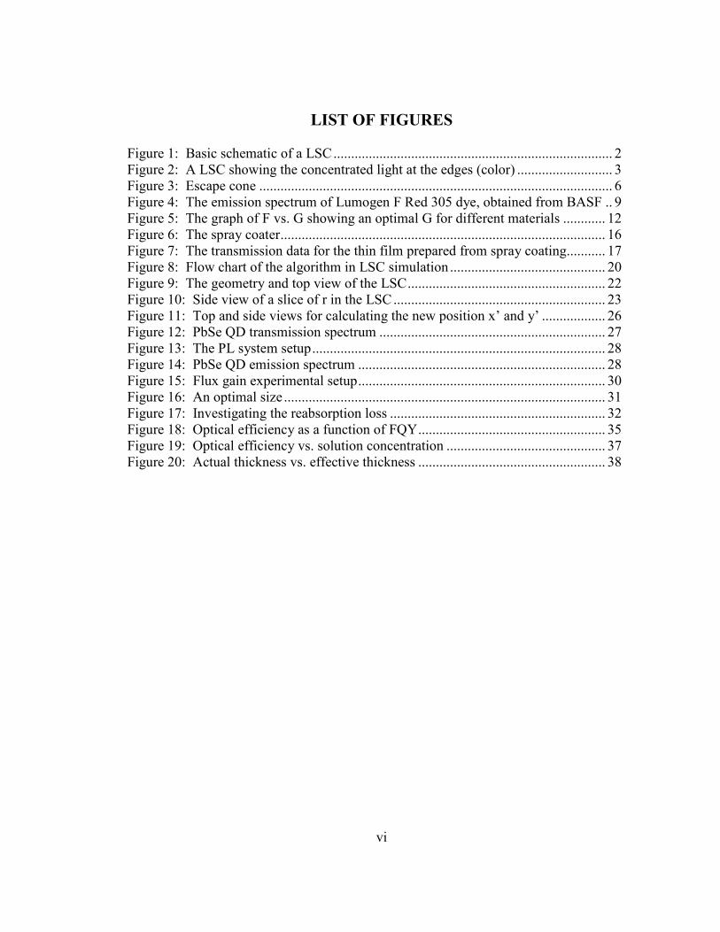
LIST OF FIGURES
Figure 1: Basic schematic of a LSC............................................................................... 2 Figure 2: A LSC showing the concentrated light at the edges (color) ........................... 3 Figure 3: Escape cone .................................................................................................... 6 Figure 4: The emission spectrum of Lumogen F Red 305 dye, obtained from BASF .. 9 Figure 5: The graph of F vs. G showing an optimal G for different materials ............ 12 Figure 6: The spray coater............................................................................................ 16 Figure 7: The transmission data for the thin film prepared from spray coating........... 17 Figure 8: Flow chart of the algorithm in LSC simulation ............................................ 20 Figure 9: The geometry and top view of the LSC........................................................ 22 Figure 10: Side view of a slice of r in the LSC............................................................ 23 Figure 11: Top and side views for calculating the new position x’ and y’ .................. 26 Figure 12: PbSe QD transmission spectrum ................................................................ 27 Figure 13: The PL system setup................................................................................... 28 Figure 14: PbSe QD emission spectrum ...................................................................... 28 Figure 15: Flux gain experimental setup...................................................................... 30 Figure 16: An optimal size ........................................................................................... 31 Figure 17: Investigating the reabsorption loss ............................................................. 32 Figure 18: Optical efficiency as a function of FQY..................................................... 35 Figure 19: Optical efficiency vs. solution concentration ............................................. 37 Figure 20: Actual thickness vs. effective thickness ..................................................... 38
vii
LIST OF TABLES
Table 1: Comparison of coating methods .................................................................... 16 Table 2: Variations of pressure and passes on thickness ............................................. 17 Table 3: Results from simple reabsorption loss experiment ........................................ 32 Table 4: Square vs. rectangular geometry.................................................................... 34 Table 5: Effect of solution concentration on optical efficiency ................................... 36

viii
ACK�OWLEDGEME�TS
I would like to thank Matt Fetterman for his collaboration in the luminescent solar concentrator simulation work. I would also like to thank GoldSim Technology Group for providing a free copy of their simulation software. The work is funded by Army Research Office.
Chapter 1
Introduction
Solar energy is a very attractive energy source because it is practically unlimited.
As the call for renewable energy is gaining momentum, solar power generation is getting
a lot more attention. Unfortunately it is still expensive to harness the sun’s power
because of the cost of solar cells. One promising candidate for reducing the cost of solar
power generation is the luminescent solar concentrator (LSC). Luminescence is the
radiation of light induced by an energy source [1]. All luminescence described here is
induced by sunlight.
The idea of using LSC as a way to reduce the cost of solar power generation first
came about around mid 1970s [2-3]. LSC has a renewed interest these days because of
the availability of new materials such as colloidal quantum dots, more efficient
fluorescent dyes, and near-IR dyes. LSC is an optical device for concentrating sunlight
into a small area of solar cells located at the edges of the LSC using fluorescent materials.
LSC has the potential of drastically cutting the cost for solar electricity generation. This
is done by replacing a large area of expensive solar cells in a solar panel with inexpensive
materials and a very small area of solar cells at the edges. An advantage this device has
over other solar concentrators is its ability to use both diffused and direct sunlight,
therefore abolishing the need of expensive sun-tracking systems. Diffused light is the
scattered sunlight after passing through the Earth’s atmosphere [4]. Also LSC only have
a very slight drop in efficiency on a cloudy day [2, 5]. This is because direct sunlight is
2
mostly blocked by the clouds and scattered, leaving mostly diffuse sunlight. Since the
LSC is an efficient diffused light absorber, its efficiency is only affected slightly [2, 5].
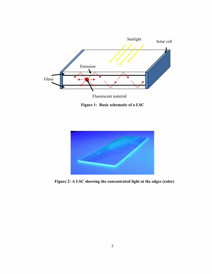
A basic LSC has fluorescent materials that absorbs sunlight and directs it towards
the small area of solar cells at the edges of the panel. Fluorescence is a type of
luminescence where the radiation emission happens over a very short period of time [1].
The typical LSC uses organic fluorescent dyes as the fluorescent materials. The biggest
advantage of this system is its lower cost than other types of LSCs and the dyes’ high
fluorescent quantum yield (FQY). This material system has the disadvantage of higher
reabsorption loss than other LSCs because of the big overlap of the dyes’ absorption and
emission spectra. It also has a low lifetime because of the dyes’ vulnerability to photo-
bleaching. An improvement over the usual type of LSC is to use fluorescent dyes in
conjunction with rare earth materials like neodymium and ytterbium [2]. This system has
lower reabsorption loss, high FQY, and high stability. But the drawback of using rare
earth materials is their low absorption coefficient, which leads to a need for much higher
solution concentration, resulting in a higher cost [6]. Another possible material system is
to use colloidal quantum dots (QDs) instead of organic fluorescent dyes. This system has
low reabsorption loss because of its narrow emission spectrum. It also has a considerably
higher lifetime than organic dyes. The disadvantages of this type of LSC are its low FQY
and the high cost of the QDs.
3
Sunlight Solar cell
Fluorescent material
Glass
Emission
Figure 1: Basic schematic of a LSC
Figure 2: A LSC showing the concentrated light at the edges (color)
Chapter 2
Theory of Operation
In this chapter, the main principles and important parameters in the operation of a
LSC will be covered. These include total internal reflection, loss through escape cone
and reabsorption, flux gain, geometric gain, optical efficiency, and external quantum
efficiency.
2.1 Absorption and emission spectrum
Absorption is the single most important parameter in a LSC. If sunlight is not
absorbed, then there will not be any emission. Therefore the first parameter to consider
should be the absorption spectrum of the fluorescent material(s). Next would be the
emission spectrum of the fluorescent material(s). It is desirable to have a narrow
emission spectrum with a large Stokes shift [7]. The Stokes shift is the shift of the
emission peak from the absorption peak. Given an identical emission spectrum, a larger
Stokes shift, i.e. a larger difference between the emission and absorption peak, means
there is less overlap between the two spectra. Furthermore, dyes or QDs can be chosen
such that their emission peaks coincide with the wavelength that maximizes the
efficiency of the solar cell at the edges, or vice versa. For a solar cell with a certain band
gap, the maximum efficiency occurs for incoming photons with energy slightly above
that of the band gap because less energy would be wasted compared to higher energy
photons.
Commercial dyes available have absorption peaks that span across the visible into
the near ultraviolet and near infrared spectrum. For a single type of dye, its absorption
5
spectrum is limited to a small part of the solar spectrum. Dyes in general also have a
broad emission spectrum, which is undesirable in a LSC. One interesting way to work
around the single dye absorption spectrum limitation is to use multiple dyes. By
combining three, or even four types of dyes, and using a principle called Forster
Resonance Energy Transfer (FRET), absorbed energy can be transferred non-radiatively
to a final emission dye [8-9].
QDs are interesting in the study of LSC because their absorption or emission
peaks can be tailored through fine-tuning their sizes. QDs such as PbSe QD have a very
broad absorption spectrum that span the whole visible and near infrared spectrum. They
also have a much narrower emission spectrum than dyes in general, which is desirable.
2.2 Fluorescence quantum yield (FQY)
FQY is a fundamental property of a fluorescent material. It is has a value
between 0 and 1, defined as the ratio of photons emitted and photons absorbed. It is the
probability of emission for every photon absorbed. It is a very important parameter in a
LSC because a low probability of emission will translate to lower efficiency. A high
FQY means that the LSC will have high efficiency. Dyes generally have high FQY
(>0.85) while QDs have relatively low FQY (~0.1 – 08). The FQY also have a slight
dependence on the solvent used, which is another consideration in a LSC.
2.3 Total internal reflection
The main working principle behind LSC is total internal reflection. Whenever a
ray of light strikes an interface between two mediums of different refractive indices at an
oblique angle larger than a certain critical angle, it will be totally and internally reflected.
6
The critical angle can be determined from Snell’s law, 2211 sinsin θθ nn = , where n1 and
n2 are the mediums’ refractive indices, and θ1 and θ2 are the incident angle and the
refraction angle, measured relative to normal. By letting n2=1 (for air), and θ2=90°, the
critical angle θc is then,
= −
2
1 1sin
ncθ .
This parameter is critical in determining one of the major loss mechanisms in LSCs.
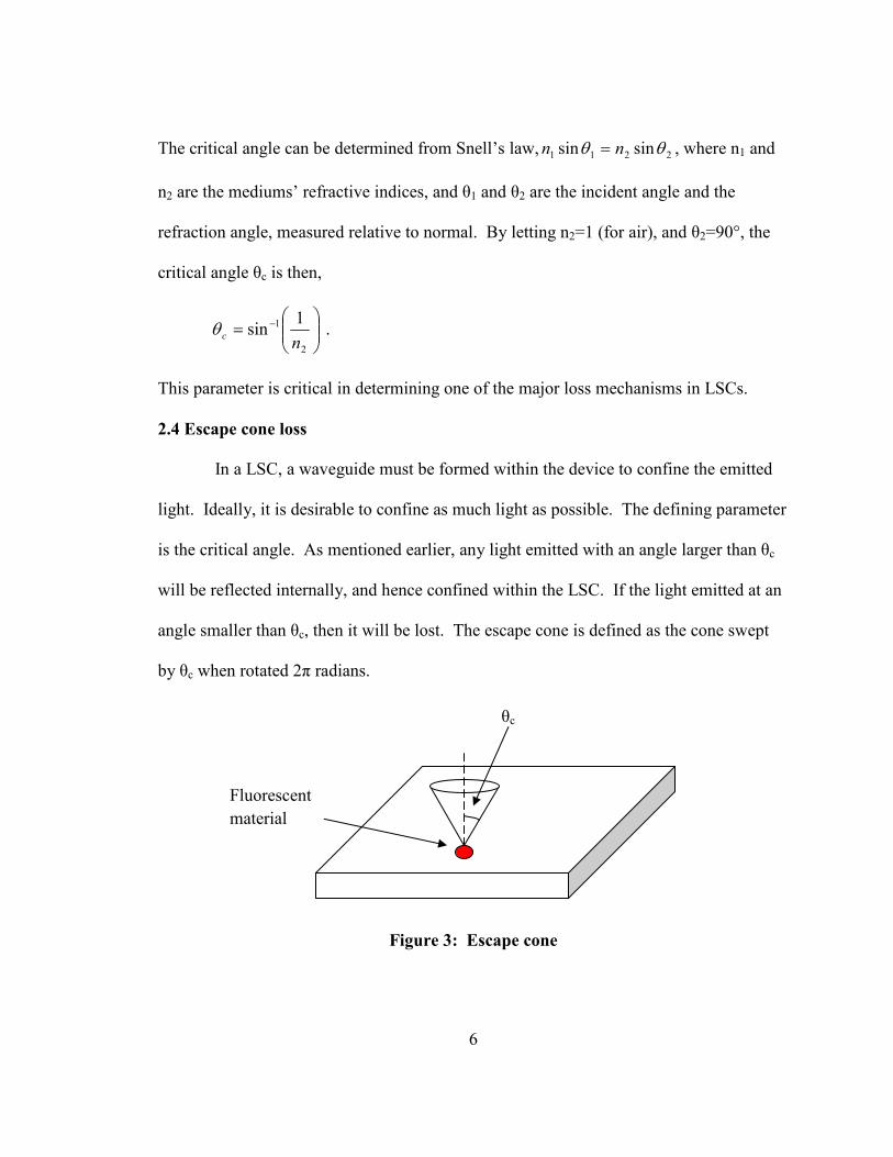
2.4 Escape cone loss
In a LSC, a waveguide must be formed within the device to confine the emitted
light. Ideally, it is desirable to confine as much light as possible. The defining parameter
is the critical angle. As mentioned earlier, any light emitted with an angle larger than θc
will be reflected internally, and hence confined within the LSC. If the light emitted at an
angle smaller than θc, then it will be lost. The escape cone is defined as the cone swept
by θc when rotated 2π radians.
θc
Fluorescent
material
Figure 3: Escape cone
7
The amount of light trapped is found by looking at the ratio of the area swept
outside of the escape cone to the area of a sphere.
θπφθθπ θπ
cos4sin 22
0 0
2 rddrAout == ∫ ∫−
Since the area of a sphere is 4πr2, the ratio is then given by cosθc. For glass with
refractive index of 1.5, θc is 41.8°, and the amount of light trapped is about 74.5%. The
escape cone is going to be determined ultimately by the material chosen to be on top of
the LSC. It is of course desirable to have a very high refractive index material, but
materials with high refractive indices (>1.8) are not available commercially. Common
inexpensive materials that are used for LSC are glass, PMMA, or PET.
One possibility of combating the escape cone loss is through a hot mirror. A hot
mirror is a coating on top of a LSC that permits the short wavelength light through at the
front surface but reflects long wavelength light at the back surface. It was suggested that
the usage of a hot mirror can provide up to 25% gain in the LSC efficiency [6]. The
downside is of course the increased cost of applying such a coating.
2.5 Reabsorption loss
Whenever a photon is emitted from the luminescent material, there is a chance
that it will be reabsorbed before it reaches the edge. It turns out that the reabsorption
process is very significant in LSC [7, 10-12].
This reabsorption is proportional to the amount of overlap between the absorption
and emission spectrum and the absorption coefficient, denoted here as α. A big overlap
will ensure a high reabsorption loss, which translates to low efficiency. This is the reason
a large Stokes shift (the shift in the emission peak with respect to the absorption peak) is
8
desirable. A parameter that is useful in looking at the reabsorption loss qualitatively is
the ratio of absorption coefficient at absorption peak to the absorption coefficient at the
emission peak [12]. Another factor that influences the reabsorption loss is the solution
concentration. While a higher solution concentration can ensure more absorption of the
incident light, it also means that the probability that an emitted photon will be reabsorbed
before reaching the edge increases exponentially. Logically there should be an optimal
solution concentration and this was confirmed in other literature [7].
The reabsorption loss can be quantified through the application of Beer-Lambert
law,
deII α−= 0 , where
I0 is the initial light intensity, α is the absorption coefficient, and d is the length
the photon has to travel. The intensity can be thought of as synonymous with the number
of photons, since the intensity is proportional to the number of photons. In essence, the
equation can ultimately describes the number of photon reaching the collecting edges,
which is important in simulation such as a ray-tracing model. The absorption coefficient
can be experimentally obtained through either a transmission or absorption measurement
with a spectrometer.
In general, QDs have relatively low reabsorption loss because of their narrow
emission spectrum. Since the spread in QDs’ emission spectrum is due mainly to the
distribution in the dot sizes, better processing methods can further narrow the emission
spectrum. Organic dyes, which generally have broader emission spectrum, have larger
reabsorption loss.
9
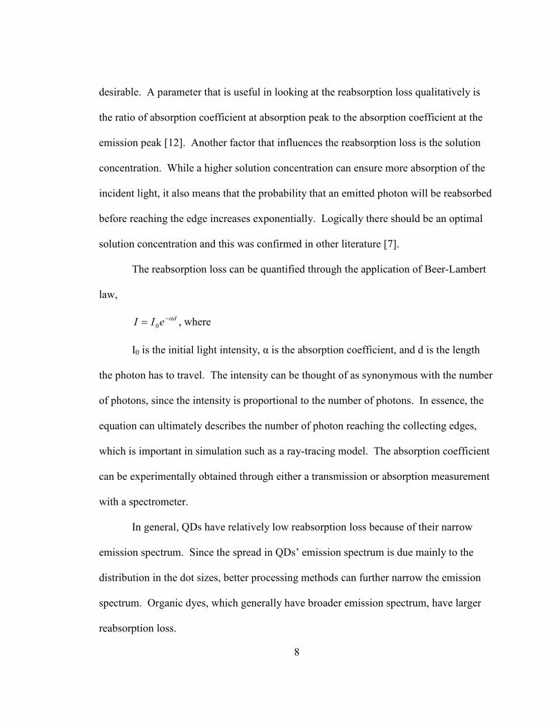
Even when the emitted photon is reabsorbed, all is not lost because there is still a
chance for it to be re-emitted again. The chance for the photon to be re-emitted has to
again take into account the fluorescent material’s FQY.
2.6 Mirrors
One way to enhance the efficiency of LSC is to use a mirror at the back. The
purpose of the mirror is to reflect light that was not absorbed in the first pass for a second
chance to be absorbed, hence increasing the absorption probability. However, since
metallic mirrors such as silver mirrors are not perfect (~7% loss), there should be an air
gap between the LSC and mirror [4, 13]. Even so, a loss of 7% is rather large
considering that usually many passes are required before the light gets to the edge.
Instead of a mirror, a white scattering layer can be used as well [13-14]. The
purpose of the white scattering layer is two-fold: to reflect the transmitted light so it can
Figure 4: The emission spectrum of Lumogen F Red 305 dye,
obtained from BASF.
10
be reabsorbed, and to redirect light that are outside of the absorption spectrum to the
collecting edges. Debije [13] has shown that the addition of a white scattering layer
increase the LSC output significantly, around 30 – 50%.
2.7 Optical efficiency and external quantum efficiency
The optical efficiency, ηopt, is defined as the fraction of photons reaching the
collecting edges. It does not take into account the efficiency of the solar cell nor the
coupling loss between the waveguide and solar cell at the edges. It is only a measure of
the material system used. The optical efficiency is useful in comparing the performances
of fluorescent materials that emit around the same wavelength. The optical efficiency is
also easier to be measured than the external quantum efficiency in specific cases [7].
The external quantum efficiency, ηEQE, defined as the number of electron
generated per photon, takes into account the solar cell efficiency and the coupling loss as
well. Unfortunately this measurement is difficult to do [14]. For a theoretical calculation
[11-12],
trapPL
trapPL
absQEEQEr
r
ηη
ηηηηη
−
−=
1
)1(, where
ηQE is the quantum efficiency of the solar cell, ηabs is the absorption probability,
ηPL is the fluorescent material’s FQY, ηtrap is the trapping efficiency, given by cosθc, and
r is the average probability that an emitted photon will be reabsorbed. The expression for
r is rather complicated, but can be simplified with a few assumptions as shown by Currie
[12]. Letting the emission spectrum be a delta function and the LSC be a square, the
average reabsorption probability, r, can be simplified to
11
c
AGExpdd
r c
θπ
φθφθθ
π
π
π
θ
cos
cossin
)10ln(2sin2
1
4/
4/
2/
−
−=
∫∫−
, where
A is the LSC absorbance at the emission peak, given by dA PLα= , and αPL is the
absorption coefficient at the emission wavelength.
Noting that all the terms after ηQE can be summarized as the optical efficiency,
optQEEQE ηηη = .
This expression yields a relatively easy way to calculate ηEQE in a simulation
where the output is the optical efficiency.
2.8 Flux gain and geometric gain
The geometry of a LSC plays an important role as well. One way to quantify the
geometry contribution is the geometric gain, G, defined as
areasideTotal
areatopTotal=G .
Naturally a high G value is desire because that would mean more cost savings.
There is a limit to G, however, because as the LSC dimensions increases, so does the
reabsorption loss. The next step is to find out the optimum value for G, and this is done
by looking at another parameter, the flux gain, F. The flux gain is a measure of how
much light is concentrated at the edge. This is the value that ultimately needs to be at its
highest because it measures how well a solar concentrator concentrates light. It is
defined as [11],
PV
concGF
ηη
= , where
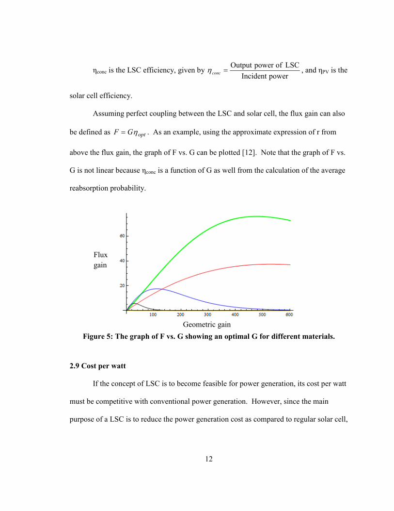
12
ηconc is the LSC efficiency, given by powerIncident
LSCofpowerOutput=concη , and ηPV is the
solar cell efficiency.
Assuming perfect coupling between the LSC and solar cell, the flux gain can also
be defined as optGF η= . As an example, using the approximate expression of r from
above the flux gain, the graph of F vs. G can be plotted [12]. Note that the graph of F vs.
G is not linear because ηconc is a function of G as well from the calculation of the average
reabsorption probability.
2.9 Cost per watt
If the concept of LSC is to become feasible for power generation, its cost per watt
must be competitive with conventional power generation. However, since the main
purpose of a LSC is to reduce the power generation cost as compared to regular solar cell,
Geometric gain
Flux
gain
Figure 5: The graph of F vs. G showing an optimal G for different materials.
13
its cost per watt must be smaller than that of the solar cell. The cost per watt can be
calculated using a simplified cost model [12],
cellsolar
$1costcollector $
+=
WFPW concLSC η
, where
P is the power of sunlight incident on LSC.
For a LSC to be practical, F must be larger than 1.
2.10 Lifetime
Another crucial factor in the LSC implementation is the device lifetime. This is
fundamentally a property of the fluorescent material because glass and polymer such as
PMMA can last for a very long time. Since the device oxidation can be minimized with
packaging, the next biggest factor (assuming near-perfect manufacturing conditions) for
device degradation is then solar radiation, more specifically around the UV portion.
Organic dyes can only last a few months under solar radiation, but with a UV-blocking
coating, a stability of many years has been reported [15-16]. QD generally have better
stability than organic dyes. Of particular interest is the exciting ability for QD to have a
dark-cycle recovery, where 30-40% of total degradation was recovered with 12 hours of
darkness [17]. This is good news because about half the day is in darkness on average.
Chapter 3
Fabrication Methods
In this chapter, different fabrication methods for the LSC will be discussed.
These include the fabrication method for thin film and liquid-filled LSC.
3.1 Thin film LSC
Thin film based LSC is of particular interest because of its ease of packaging and
its potential on flexible substrates. Three ways for deposition of a thin film will be
discussed. Two main important properties that need to be considered are its thickness
and surface uniformity. If the sample is too thin, then most light will pass right through it.
If the sample surface is too rough, then the LSC performance will suffer because the thin
film will not form a good waveguide. Also of importance is the host matrix material.
The host matrix must be clear (to allow light to reach the fluorescent material), cheap,
and does not have significant absorption in the fluorescent material working spectrum.
An example of a material that satisfies those conditions is poly(methyl methacrylate)
(PMMA), or more commonly known as acrylic glass.
3.1.1 Spin coating
Spin coating is popular for creating thin films on the order of 10 – 100 nm
thickness because it is generally consistent in creating good quality films. It can also be
done fairly quickly and easily. A spin coater works by holding the substrate in place via
a vacuum and spinning the solution-covered substrate at a high rate of speed.
Spin coating is great for applications where really thin films are needed but not for LSC.
For films on the order of 100 nm, the transmission is generally more than 90%. This
15
means that less than 10% of the incoming light will be absorbed, bringing the maximum
theoretical efficiency to less than 10%. As such, spin coating is a bad candidate for
creating a thin film LSC.
3.1.2 Dip coating
Dip coating is another method popular in creating thin film devices. A dip coater
works by submerging the substrate in a bath of solution and slowly lifting it up through a
stepper motor. Unfortunately, a thin film made by a dip coater has around the same
characteristic as a spin coated film. This means that it is limited in capabilities with
respect to LSC as a spin coater.
3.1.3 Spray coating
Another way to create a thin film is through spray coating. It works by spraying
the target solution layer by layer onto a cleaned substrate, very much like the spray
painting done in outdoor painting. Films created by this method can have a thickness on
the order of microns and surprisingly smooth surfaces. Since the film thickness is about
100 thicker than that of films created by the other two methods, spray coating might be a
feasible method for creating thin film LSC. The downside of this method is the user.
Since the film application is not automated by a machine, irregularities of film
thicknesses and quality will vary over a big range. It is speculated that it is possible to
minimize this variation by automating this process. One interesting way to improve the
film quality was by first spin coating a layer of thin film on the substrate before spray
coating.
16
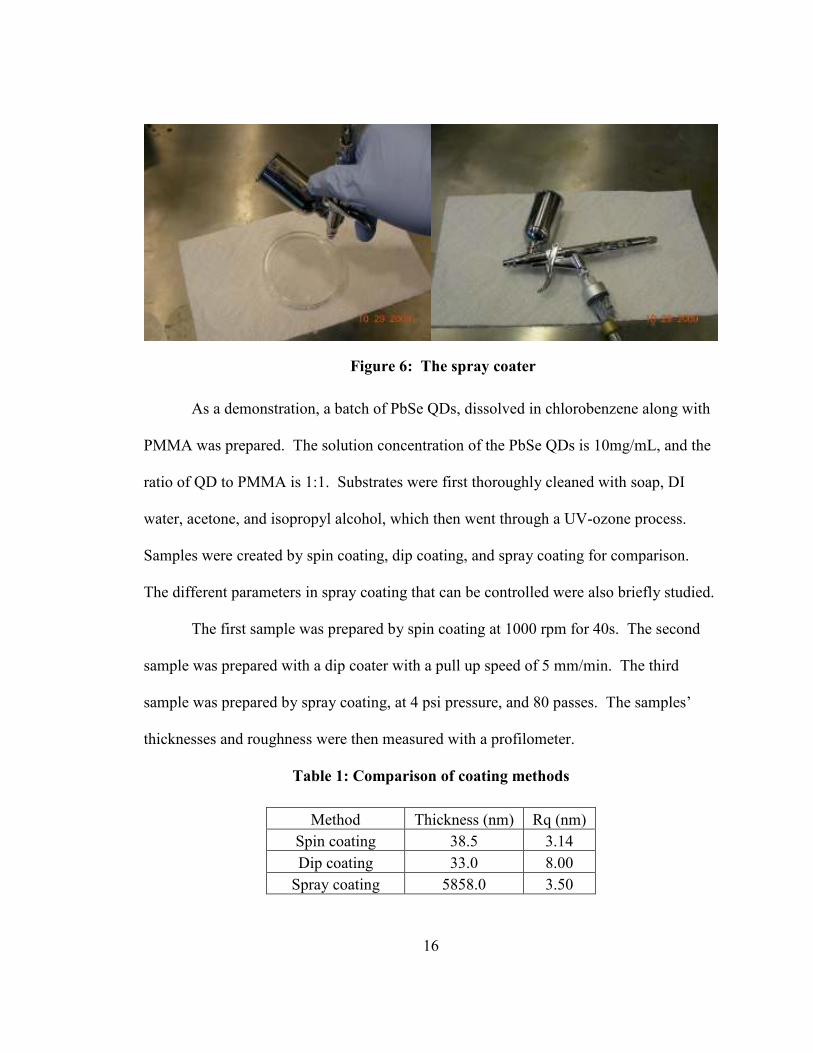
As a demonstration, a batch of PbSe QDs, dissolved in chlorobenzene along with
PMMA was prepared. The solution concentration of the PbSe QDs is 10mg/mL, and the
ratio of QD to PMMA is 1:1. Substrates were first thoroughly cleaned with soap, DI
water, acetone, and isopropyl alcohol, which then went through a UV-ozone process.
Samples were created by spin coating, dip coating, and spray coating for comparison.
The different parameters in spray coating that can be controlled were also briefly studied.
The first sample was prepared by spin coating at 1000 rpm for 40s. The second
sample was prepared with a dip coater with a pull up speed of 5 mm/min. The third
sample was prepared by spray coating, at 4 psi pressure, and 80 passes. The samples’
thicknesses and roughness were then measured with a profilometer.
Table 1: Comparison of coating methods
Method Thickness (nm) Rq (nm)
Spin coating 38.5 3.14
Dip coating 33.0 8.00
Spray coating 5858.0 3.50
Figure 6: The spray coater
17
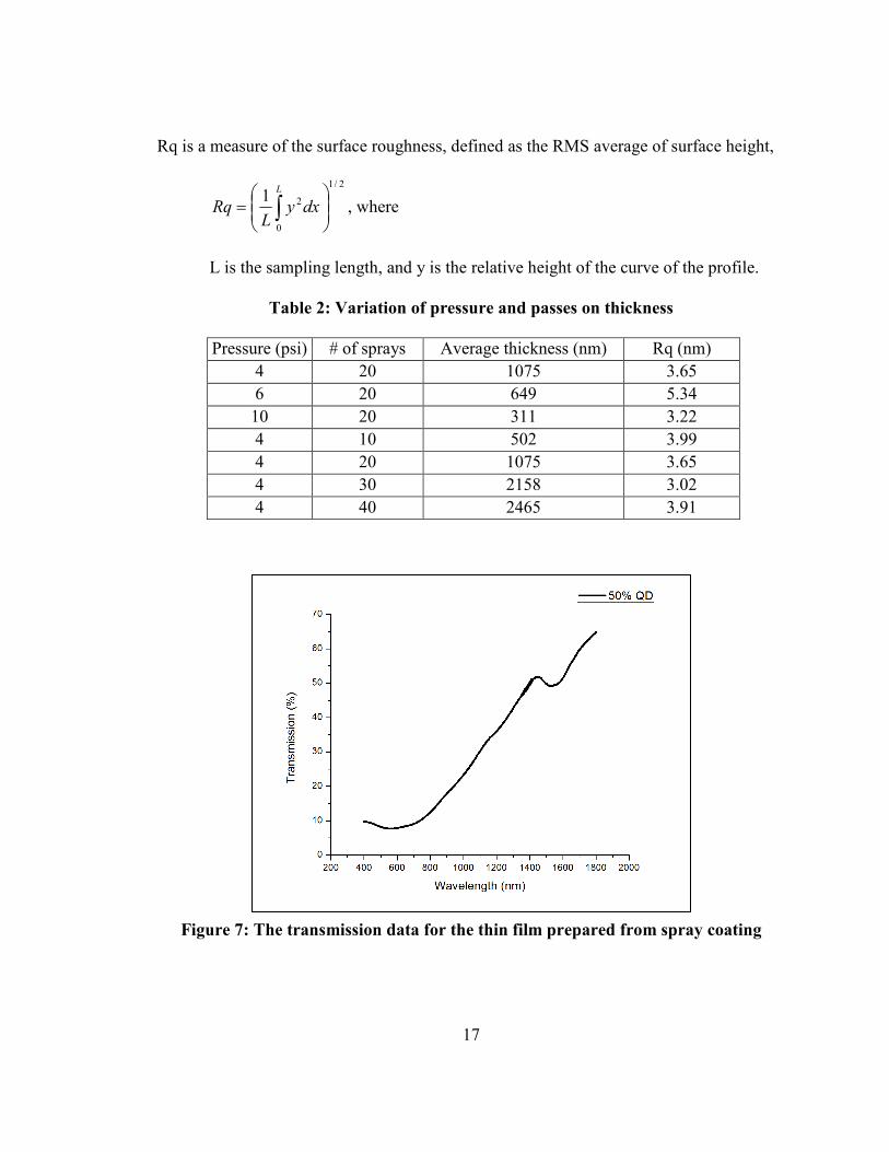
Rq is a measure of the surface roughness, defined as the RMS average of surface height,
2/1
0
21
= ∫
L
dxyL
Rq , where
L is the sampling length, and y is the relative height of the curve of the profile.
Table 2: Variation of pressure and passes on thickness
Pressure (psi) # of sprays Average thickness (nm) Rq (nm)
4 20 1075 3.65
6 20 649 5.34
10 20 311 3.22
4 10 502 3.99
4 20 1075 3.65
4 30 2158 3.02
4 40 2465 3.91
Figure 7: The transmission data for the thin film prepared from spray coating
18
As can be seen from Table 1, the spray coating method yields a film thickness of
more than 150 times than the spin coating method, while still maintaining similar
roughness. The two things that can be controlled in the spray coater was the pressure and
how many layers to apply. A low pressure is desirable because the high pressure will
blow the solution away from the substrate. An important determination of the roughness
is the substrate condition. The substrate must be cleaned thoroughly to ensure good
quality film. From an ellipsometry measurement, the film refractive index was estimated
to be around 1.51. Overall the spray coating method is definitely a feasible method to
prepared thin film LSC because of the ability to deposit micron-thickness films and it is
fairly inexpensive.
3.2 Liquid-filled LSC
Instead of a thin film, LSC can also be prepared as a liquid-filled, or solution
based LSC. This is usually done by molding glass together through optical epoxy, filling
it with the sample solution, and closing the opening with optical epoxy. This is also the
most common way to prepare LSC by far.
The solution LSC is also generally more efficient than thin film LSC because
dyes and QDs generally have higher FQY in solution. It is also easier to make because
there is no host matrix and film quality to be concerned of. For a given material, only the
solution concentration and the LSC thickness play an important role in the determining
the device performance.
Chapter 4
Monte Carlo Simulation Based on Ray Tracing Model
A simulation program can be invaluable in the work of LSC because it allows for
tweaking of different parameters with ease to their optimal values. There are already two
main methods that were developed to handle LSC simulation. The first one is a
thermodynamic model and the second is a ray tracing model.
A QD based simulation was already developed by Gallagher [18]. She simulated
large quantities (> 1 billion) of individual QDs in her model. This can lead to a
computationally exhaustive procedure. Sholin [7] and Burgers [19] also developed
different ray-tracing program, but since programs such as these are difficult to obtain, a
new program must be written from scratch to model a LSC.
A Monte Carlo simulation based on ray-tracing model was chosen. It is a
statistical model that tracks the progression of photons and applies ray principles [19],
such as Snell’s law and Beer-Lambert law, as the photons travel in the LSC. Whenever
there are different ways for the progression of the photons, random numbers are
generated to determine the photons’ fate, such as path length, emission angles, etc. The
program that was used to handle the Monte Carlo simulation is GoldSim, provided for
free by GoldSim Technology Group.
4.1 Assumptions
There are some assumptions that were made to simplify the calculation, and hence
the program.
1. The QDs in the solution are assumed to be homogeneously dispersed.
20
2. The solution is assumed to have the same refractive index as glass.
3. The interface between the solution and glass is assumed to be perfect.
4. At the interface between the glass and air, a photon is either trapped or lost
through escape cone, i.e. no partial reflection within the escape cone.
5. All incident light on the LSC is normal to the top plane.
6. All incident light is not reflected off the top surface.
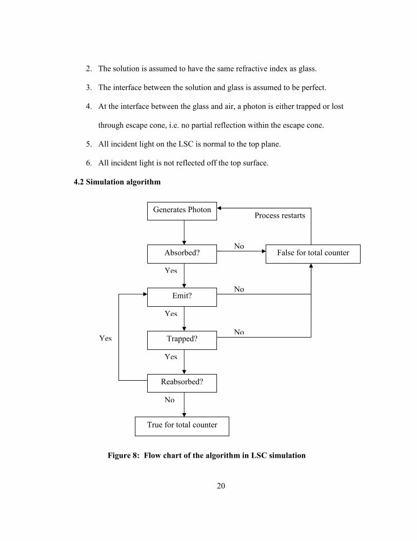
4.2 Simulation algorithm
Generates Photon
Absorbed?
Emit?
True for total counter
Trapped?
Reabsorbed?
False for total counter
Yes
Yes
Yes
Yes
No
No
No
No
Process restarts
Figure 8: Flow chart of the algorithm in LSC simulation
21
A flow chat, based on work by Sholin [4], representing the simulation algorithm
is presented above. A random number generator is used to assign a wavelength to the
photon according to the probability density function associated with the light source
(AM1.5 spectrum for sunlight).
The photon then has a chance to be absorbed by the QD. This chance of
absorption can be obtained experimentally from a transmission measurement for different
wavelengths. From the transmission measurement, the absorption coefficient can be
obtained as well. The transmission, T, is given by deI
IT α−==
0
. Solving for α yields
d
T )ln(−=α , where
d is the thickness of the cuvette used in the transmission measurement.
Once the photon is absorbed, it then has a chance to be emitted. The probability
of emission is given by the QD’s FQY, which can be obtained either experimentally or
from sources such as the manufacturer of the QD.
Whenever there is emission, two angles, θ and ϕ, are randomly generated and
assigned as the emission angle. The two angles are chosen from uniform distributions
because the QD emission is omnidirectional. Only the angle θ is taken into account in the
calculation for the trapping. If the angle θ is greater than θc, then the photon is trapped
inside the LSC.
As mentioned before, each emitted photon has a chance of being reabsorbed
before it reaches the collecting edges. If it is not reabsorbed, then the program adds one
22
to the total counter. If it is reabsorbed, then the program loops back to the emission
process for another chance to be re-emitted at two new angles.
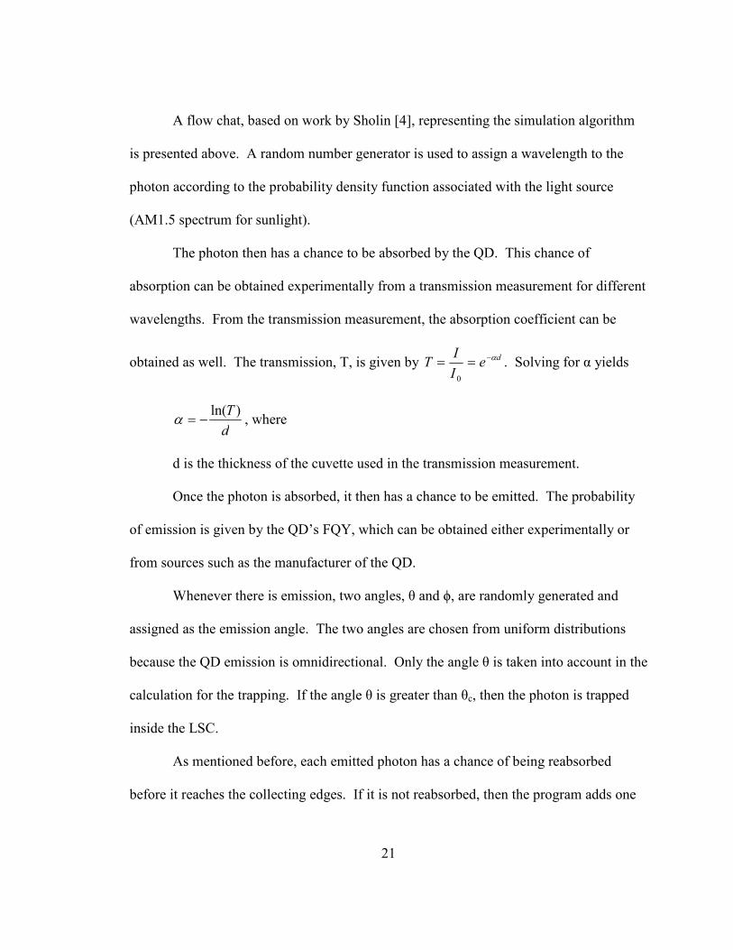
The process for calculating the reabsorption is slightly more complex than the
other processes. Given a random position, (x, y), where the photon is absorbed in the
LSC, two random emission angles, θ and ϕ, the width, and the length of the LSC, the
total path length needed to reach the collecting edge needs to be found. The idea then is
to use the Beer-Lambert equation but it only describes absorption in one dimension. The
z
y
x
θ
ϕ
W
t
L (0, 0, 0)
Top View
x
y
(x, y)
(0, 0)
x W-x
y
L-y r
ϕ
Figure 9: The geometry and top view of the LSC
23
first step then is to break down the three dimensional problem into a one dimensional
problem.
The top of the LSC is split into four quadrants, indicated by the dashed line
touching the corners. It is easier to express the length r through conditional statements
because the expression can be found easily.
For
−−
≤≤ −
xW
yL1tan0 φ and
−
−°≥ −
xW
y1tan360φ , φcos
xWr
−= .
For
−−°≤≤
−− −−
x
yL
xW
yL 11 tan180tan φ , φsin
yLr
−= .
For
−°≤≤
−−° −−
y
x
x
yL 11 tan270tan180 φ , φcos
xr = .
For
−
−°≤≤
−° −−
xW
y
y
x 11 tan360tan270 φ , φsin
yr = .
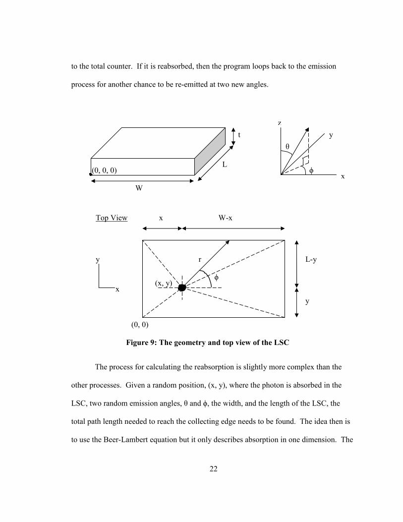
Once r is determined, the total path length to the edge can be found by looking at
the side view of a slice of r. The total path length, lT, is given by
Side View
r
z
t-z θ θ θ θ
Figure 10: Side view of a slice of r in the LSC
24
θsin
rlT = .
For a given set of six parameters stated earlier, the total path length to the
collecting edge is fixed. From the assumption about the partial reflection, θ is always
more than 0°, so the case of dividing by zero is not a cause for worry. Interestingly,
when it comes to the total path length, the z coordinate and the thickness do not matter in
the calculation.
Another parameter that needs to be determined before the reabsorption calculation
is the length the photon will travel, denoted as l. This is a randomly assigned number
based on a distribution. Starting from Beer-Lambert law, deII α−= 0 , the probability of
photons arriving between two lengths l2 and l1 is Exp(-αl2) – Exp(-αl1). The probability
density is then ( ) ( )
12
12
ll
lExplExp
−
−−− αα. Taking the limit as ∆l approaches zero yields a
derivative. The probability density function, P, is then given by
( ) ( ) ( )[ ] ( )lExpdl
lExpd
l
lExplExpP
lαα
ααα−=
−=
∆
−−−=
→∆
12
0lim .
Once P is determined, a random l is generated and compared to lT. If l ≥ lT, then
the photon reaches the collecting edges. If l < lT, then the photon is reabsorbed. The
photon then has a chance to be emitted again taking in account the QD’s FQY. If a
photon is not re-emitted, then the process starts all over from step one again. When a
photon is indeed re-emitted, then the new position where that occurred needs to be
determined.
25
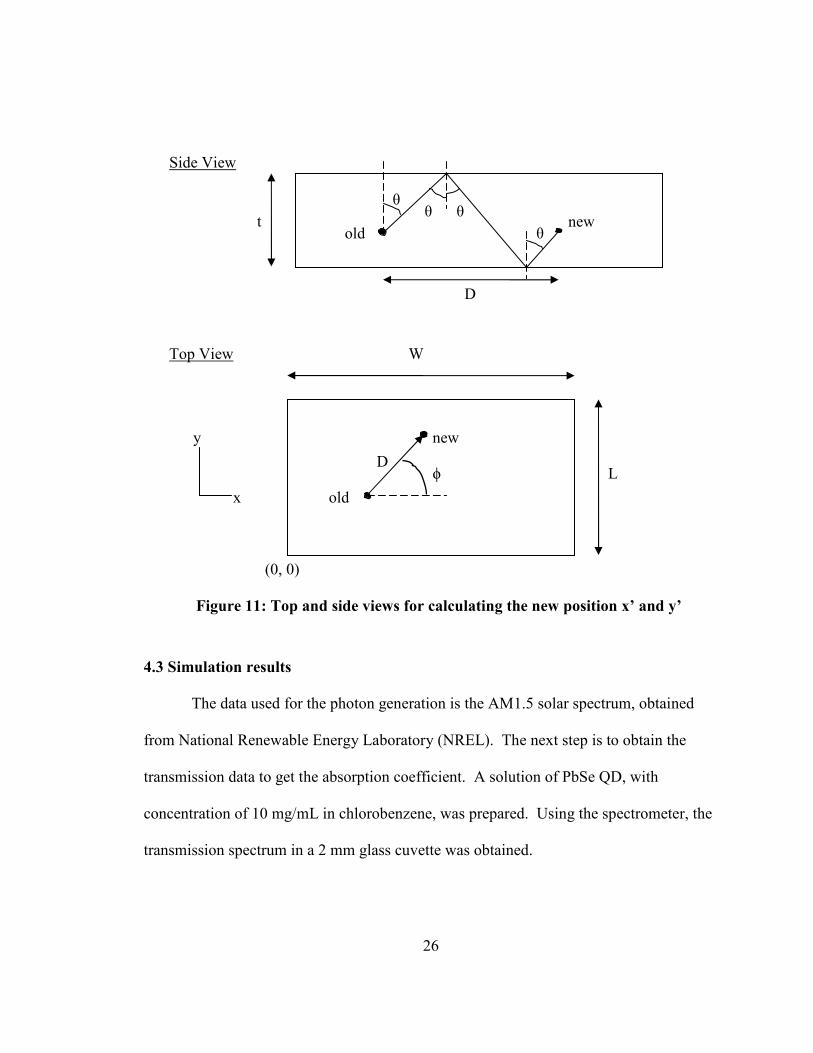
Referring to Figure 11, the length D is given by ( )θsinlD = . The new coordinate
is then
( ) ( )φφ sin,cos',' DyDxyx ++= .
Starting with the new position (x’, y’), two new angles θ’ and ϕ’ are randomly
chosen assigned, a new total path length to edge lT’ is calculated, and a new l’ is assigned
from the probability density function, and the whole process, starting from the re-
emission, starts over again.
The whole process is repeated N number of times. Since N and the total number
of “True” in the counter are known, the optical efficiency of the LSC is then given by
N
Trueof#=optη .
26
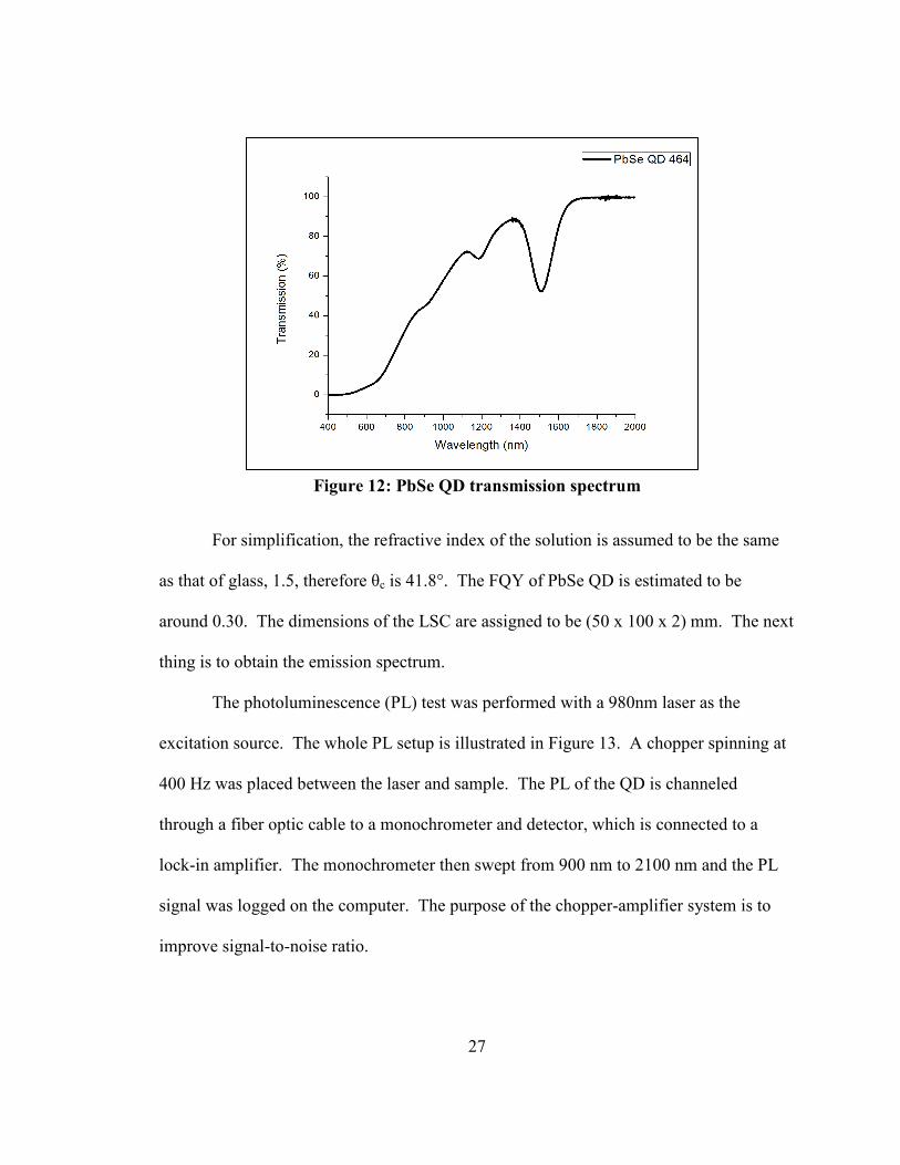
4.3 Simulation results
The data used for the photon generation is the AM1.5 solar spectrum, obtained
from National Renewable Energy Laboratory (NREL). The next step is to obtain the
transmission data to get the absorption coefficient. A solution of PbSe QD, with
concentration of 10 mg/mL in chlorobenzene, was prepared. Using the spectrometer, the
transmission spectrum in a 2 mm glass cuvette was obtained.
Side View
D
t
θ θ θ
θ old new
Top View
x
y
old
(0, 0)
W
L D
ϕ
new
Figure 11: Top and side views for calculating the new position x’ and y’
27
For simplification, the refractive index of the solution is assumed to be the same
as that of glass, 1.5, therefore θc is 41.8°. The FQY of PbSe QD is estimated to be
around 0.30. The dimensions of the LSC are assigned to be (50 x 100 x 2) mm. The next
thing is to obtain the emission spectrum.
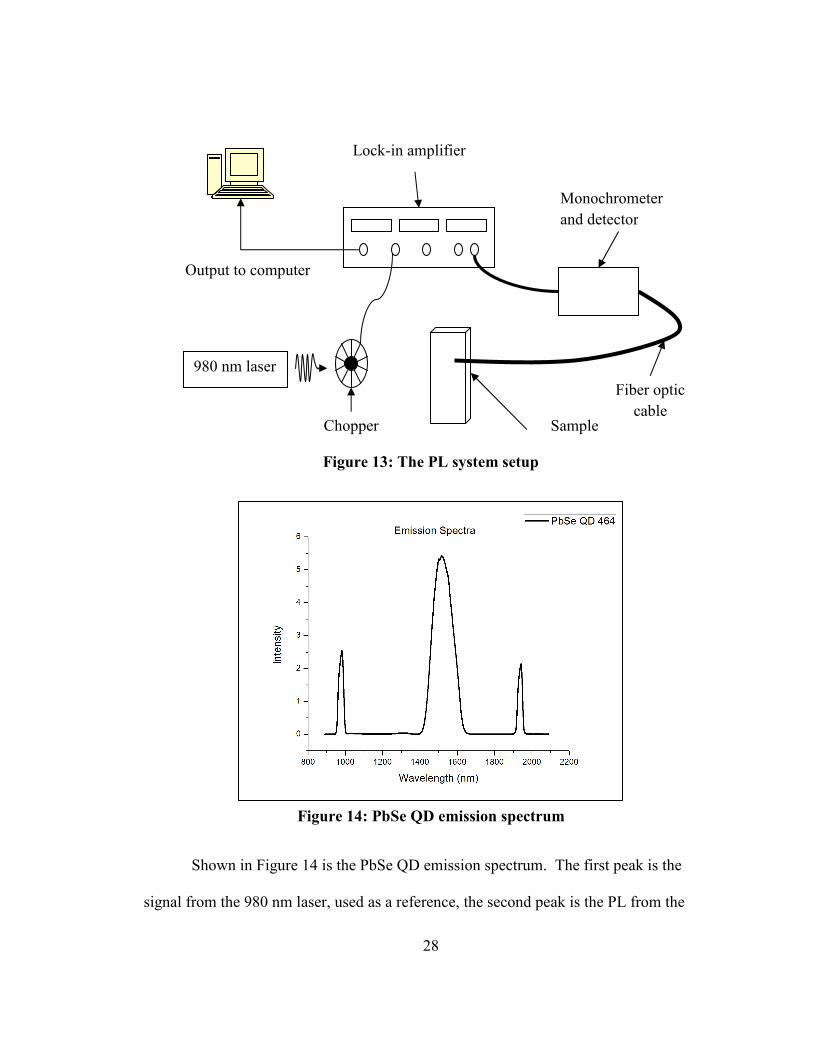
The photoluminescence (PL) test was performed with a 980nm laser as the
excitation source. The whole PL setup is illustrated in Figure 13. A chopper spinning at
400 Hz was placed between the laser and sample. The PL of the QD is channeled
through a fiber optic cable to a monochrometer and detector, which is connected to a
lock-in amplifier. The monochrometer then swept from 900 nm to 2100 nm and the PL
signal was logged on the computer. The purpose of the chopper-amplifier system is to
improve signal-to-noise ratio.
Figure 12: PbSe QD transmission spectrum
28
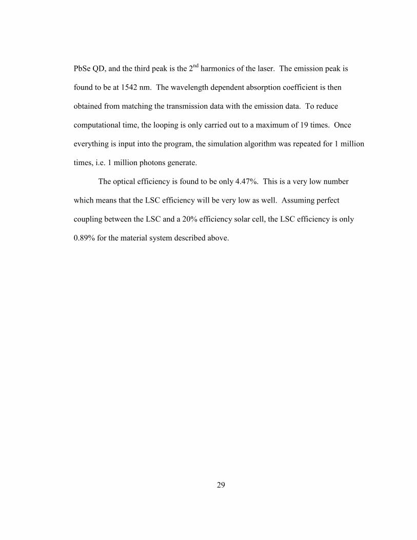
Shown in Figure 14 is the PbSe QD emission spectrum. The first peak is the
signal from the 980 nm laser, used as a reference, the second peak is the PL from the
Figure 14: PbSe QD emission spectrum
980 nm laser
Chopper Sample
Lock-in amplifier
Output to computer
Monochrometer
and detector
Fiber optic
cable
Figure 13: The PL system setup
29
PbSe QD, and the third peak is the 2nd harmonics of the laser. The emission peak is
found to be at 1542 nm. The wavelength dependent absorption coefficient is then
obtained from matching the transmission data with the emission data. To reduce
computational time, the looping is only carried out to a maximum of 19 times. Once
everything is input into the program, the simulation algorithm was repeated for 1 million
times, i.e. 1 million photons generate.
The optical efficiency is found to be only 4.47%. This is a very low number
which means that the LSC efficiency will be very low as well. Assuming perfect
coupling between the LSC and a 20% efficiency solar cell, the LSC efficiency is only
0.89% for the material system described above.
Chapter 5
Additional Experiments
Some brief experiments were conducted to verify a few details about LSC
operation.
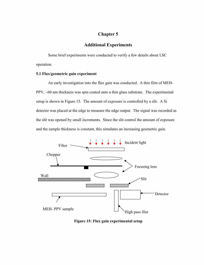
5.1 Flux/geometric gain experiment
An early investigation into the flux gain was conducted. A thin film of MEH-
PPV, ~60 nm thickness was spin coated onto a thin glass substrate. The experimental
setup is shown in Figure 15. The amount of exposure is controlled by a slit. A Si
detector was placed at the edge to measure the edge output. The signal was recorded as
the slit was opened by small increments. Since the slit control the amount of exposure
and the sample thickness is constant, this simulates an increasing geometric gain.
Figure 15: Flux gain experimental setup
Focusing lens
Chopper
Filter Incident light
Slit
MEH- PPV sample High pass filer
Detector
Wall
31
0.0
20.0
40.0
60.0
80.0
100.0
120.0
140.0
160.0
180.0
0.000 0.050 0.100 0.150 0.200 0.250 0.300
Slit opening (cm)
Sig
na
l (u
V)
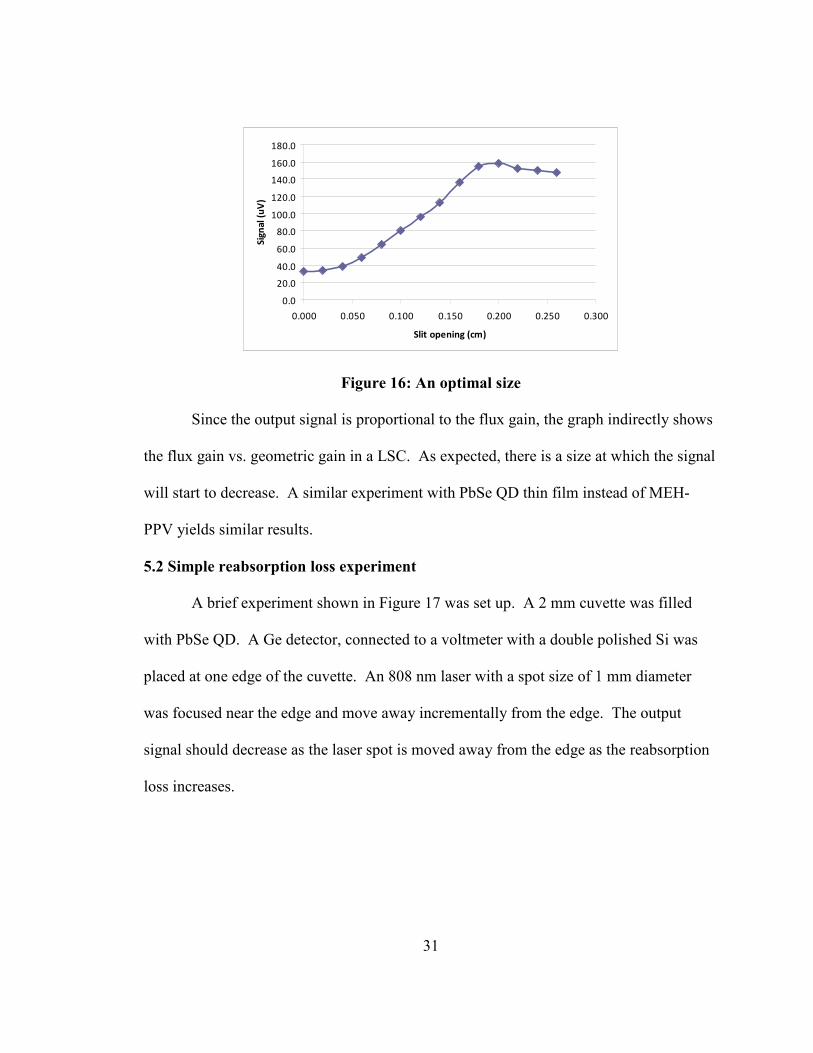
Figure 16: An optimal size
Since the output signal is proportional to the flux gain, the graph indirectly shows
the flux gain vs. geometric gain in a LSC. As expected, there is a size at which the signal
will start to decrease. A similar experiment with PbSe QD thin film instead of MEH-
PPV yields similar results.
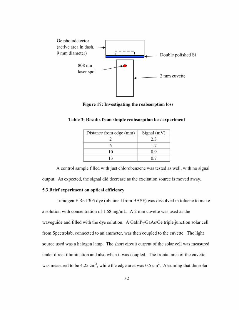
5.2 Simple reabsorption loss experiment
A brief experiment shown in Figure 17 was set up. A 2 mm cuvette was filled
with PbSe QD. A Ge detector, connected to a voltmeter with a double polished Si was
placed at one edge of the cuvette. An 808 nm laser with a spot size of 1 mm diameter
was focused near the edge and move away incrementally from the edge. The output
signal should decrease as the laser spot is moved away from the edge as the reabsorption
loss increases.
32
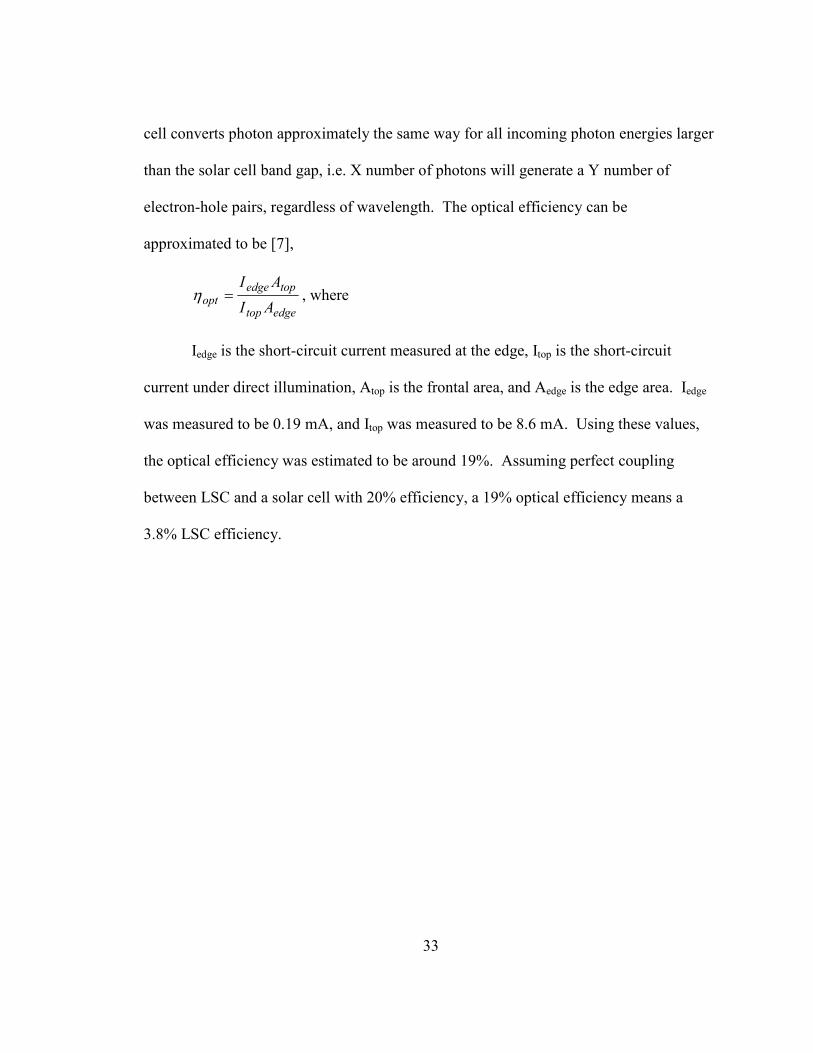
Table 3: Results from simple reabsorption loss experiment
A control sample filled with just chlorobenzene was tested as well, with no signal
output. As expected, the signal did decrease as the excitation source is moved away.
5.3 Brief experiment on optical efficiency
Lumogen F Red 305 dye (obtained from BASF) was dissolved in toluene to make
a solution with concentration of 1.68 mg/mL. A 2 mm cuvette was used as the
waveguide and filled with the dye solution. A GaInP2/GaAs/Ge triple junction solar cell
from Spectrolab, connected to an ammeter, was then coupled to the cuvette. The light
source used was a halogen lamp. The short circuit current of the solar cell was measured
under direct illumination and also when it was coupled. The frontal area of the cuvette
was measured to be 4.25 cm2, while the edge area was 0.5 cm2. Assuming that the solar
Distance from edge (mm) Signal (mV)
2 2.3
6 1.7
10 0.9
13 0.7
Figure 17: Investigating the reabsorption loss
Ge photodetector
(active area in dash,
9 mm diameter) Double polished Si
2 mm cuvette
808 nm
laser spot
33
cell converts photon approximately the same way for all incoming photon energies larger
than the solar cell band gap, i.e. X number of photons will generate a Y number of
electron-hole pairs, regardless of wavelength. The optical efficiency can be
approximated to be [7],
edgetop
topedgeopt
AI
AI=η , where
Iedge is the short-circuit current measured at the edge, Itop is the short-circuit
current under direct illumination, Atop is the frontal area, and Aedge is the edge area. Iedge
was measured to be 0.19 mA, and Itop was measured to be 8.6 mA. Using these values,
the optical efficiency was estimated to be around 19%. Assuming perfect coupling
between LSC and a solar cell with 20% efficiency, a 19% optical efficiency means a
3.8% LSC efficiency.
Chapter 6
Discussion
Using the simulation model above, the effect of a few selected parameters on the
LSC performance will be discussed in this chapter. These parameters are the geometry,
FQY, and solution concentration. A feasibility study for the LSC will be discussed as
well.
6.1 Geometry
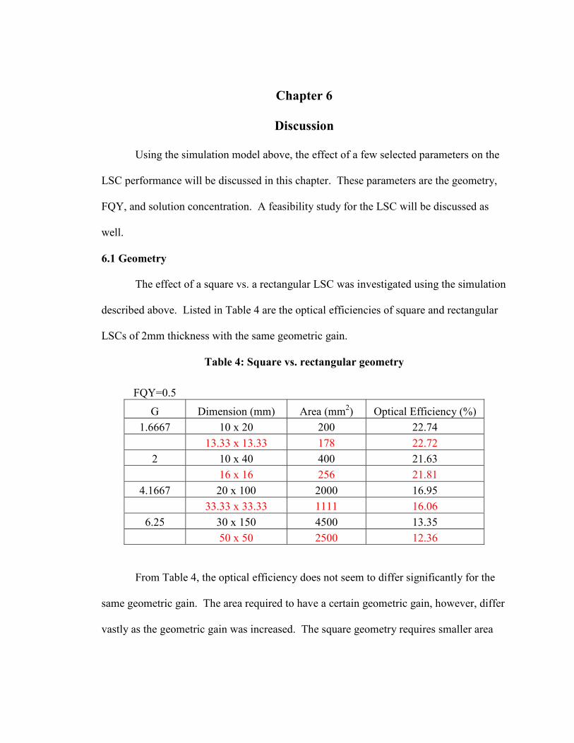
The effect of a square vs. a rectangular LSC was investigated using the simulation
described above. Listed in Table 4 are the optical efficiencies of square and rectangular
LSCs of 2mm thickness with the same geometric gain.
Table 4: Square vs. rectangular geometry
From Table 4, the optical efficiency does not seem to differ significantly for the
same geometric gain. The area required to have a certain geometric gain, however, differ
vastly as the geometric gain was increased. The square geometry requires smaller area
FQY=0.5
G Dimension (mm) Area (mm2) Optical Efficiency (%)
1.6667 10 x 20 200 22.74
13.33 x 13.33 178 22.72
2 10 x 40 400 21.63
16 x 16 256 21.81
4.1667 20 x 100 2000 16.95
33.33 x 33.33 1111 16.06
6.25 30 x 150 4500 13.35
50 x 50 2500 12.36
35
for the same geometric gain compared to the rectangular geometry. A smaller area
required translates to a cheaper LSC. Therefore a square geometry is definitely better
because it will be cheaper to manufacture a LSC of the same geometric gain compared to
a rectangular geometry.
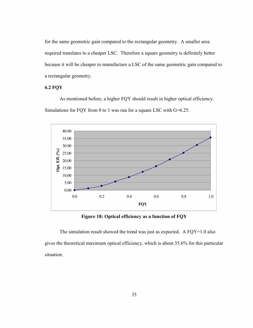
6.2 FQY
As mentioned before, a higher FQY should result in higher optical efficiency.
Simulations for FQY from 0 to 1 was run for a square LSC with G=6.25.
The simulation result showed the trend was just as expected. A FQY=1.0 also
gives the theoretical maximum optical efficiency, which is about 35.6% for this particular
situation.
0.00
5.00
10.00
15.00
20.00
25.00
30.00
35.00
40.00
0.0 0.2 0.4 0.6 0.8 1.0
FQY
Op
t. E
ff. (%
)
Figure 18: Optical efficiency as a function of FQY
36
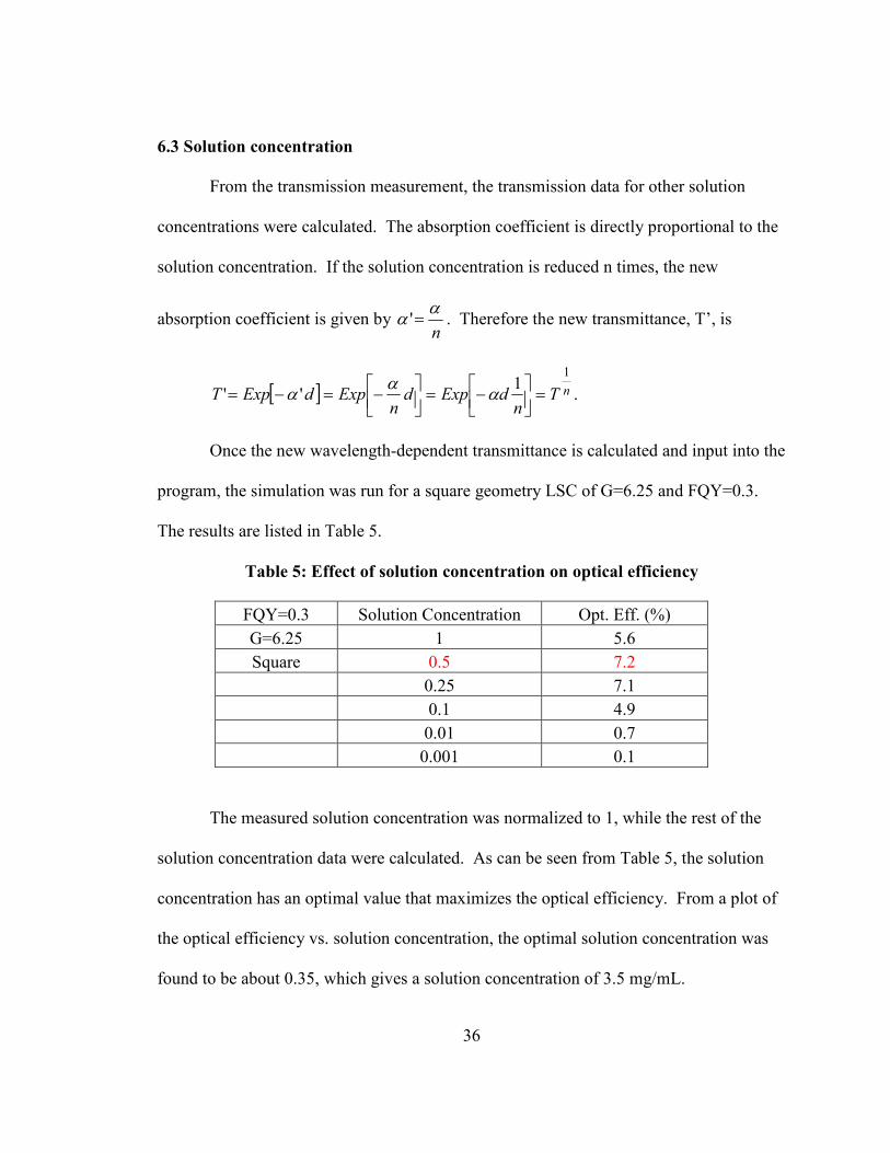
6.3 Solution concentration
From the transmission measurement, the transmission data for other solution
concentrations were calculated. The absorption coefficient is directly proportional to the
solution concentration. If the solution concentration is reduced n times, the new
absorption coefficient is given by n
αα =' . Therefore the new transmittance, T’, is
[ ] nTn
dExpdn
ExpdExpT
11
'' =
−=
−=−= αα
α .
Once the new wavelength-dependent transmittance is calculated and input into the
program, the simulation was run for a square geometry LSC of G=6.25 and FQY=0.3.
The results are listed in Table 5.
Table 5: Effect of solution concentration on optical efficiency
FQY=0.3 Solution Concentration Opt. Eff. (%)
G=6.25 1 5.6
Square 0.5 7.2
0.25 7.1
0.1 4.9
0.01 0.7
0.001 0.1
The measured solution concentration was normalized to 1, while the rest of the
solution concentration data were calculated. As can be seen from Table 5, the solution
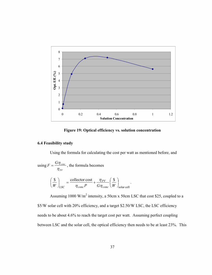
concentration has an optimal value that maximizes the optical efficiency. From a plot of
the optical efficiency vs. solution concentration, the optimal solution concentration was
found to be about 0.35, which gives a solution concentration of 3.5 mg/mL.
37
6.4 Feasibility study
Using the formula for calculating the cost per watt as mentioned before, and
usingPV
concGF
ηη
= , the formula becomes
cellsolar
$costcollector $
+=
WGPW conc
PV
concLSC ηη
η.
Assuming 1000 W/m2 intensity, a 50cm x 50cm LSC that cost $25, coupled to a
$5/W solar cell with 20% efficiency, and a target $2.50/W LSC, the LSC efficiency
needs to be about 4.6% to reach the target cost per watt. Assuming perfect coupling
between LSC and the solar cell, the optical efficiency then needs to be at least 23%. This
Figure 19: Optical efficiency vs. solution concentration
0
1
2
3
4
5
6
7
8
0 0.2 0.4 0.6 0.8 1 1.2
Solution Concentration
Op
t. E
ff. (%
)
38
is a very high number considering the LSC size. Therefore the LSC is still not a feasible
idea using the PbSe QDs discussed above.
It is speculated that better manufacturing processes can further narrow the
emission spectrum and increase the FQY of QDs. Also with mass production, it is
estimated that the collector cost will be driven down significantly. Therefore it is
speculated that it could still be feasible for QDs to be used in the LSC design.
6.5 Other factors
As mentioned previously, it was assumed that all the emitted photons within the
escape cone were totally lost. Within the escape cone, there is a chance that the emitted
photons could be “saved”. At the LSC-air interface, there is a chance that the emitted
photon will be reflected. There is also the chance of reabsorption within the escape cone.
Since the LSC thickness is very small, this reabsorption term is very small as well. While
small, including these contributions from reflection and reabsorption can make the model
more accurate.
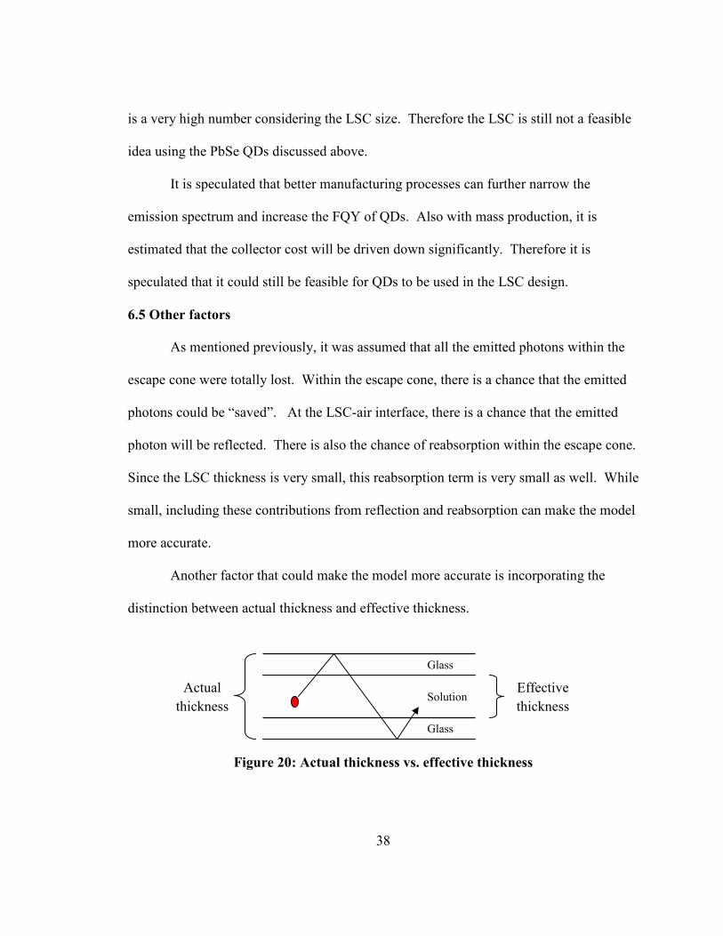
Another factor that could make the model more accurate is incorporating the
distinction between actual thickness and effective thickness.
Actual
thickness
Effective
thickness
Figure 20: Actual thickness vs. effective thickness
Glass
Solution
Glass
39
Reabsorption only occurs within the solution. Therefore the path length before
the photon is reabsorbed will be increased slightly, and hence the optical efficiency will
be increased slightly.
6.6 Solar cell at the edges
Since the LSC thickness is small, the attached solar cell must have small
dimension as well. The attached solar cell can be laser-cut from larger solar cells and
attached to the edge through a refractive index matching optical coupling [14, 19].
Instead of a regular solar cell that has front and back electrical contacts, one can instead
use a solar cell with both electrical contacts at the back, called a point contact solar cell
[20-21]. This has the benefit of reduced shading loss due to the absence of the front
electrical contact.
Chapter 7
Conclusions
7.1 Accomplished work
A simple Monte Carlo simulation based on ray tracing model has been developed.
It was found that a square geometry is more desirable over a rectangular geometry
because of the smaller area required to achieve the same effect. Also it was demonstrated
that an optimal solution concentration can be found using the simulation. It was found
that using the current PbSe QDs material system, it is still not feasible to use the LSC for
cost reduction in solar electricity generation.
7.2 Future work
The simulation model can definitely be improved to be more accurate and take
into account more factors. Since the addition of mirror will increase the optical
efficiency a lot, the first thing that needs to be included is the addition of mirrors or a
white scattering layer. Then the effective thickness needs to be taken into account as well.
Since the contributions from the reflection of the LSC-air interface and reabsorption
within the escape cone are relatively small, those two factors will be taken into account
the last.
References
[1] A. Kitai, Luminescent Materials and Applications, John Wiley & Sons, West
Sussex, England, 2008
[2] W.H. Weber, J. Lambe, Luminescent greenhouse collector for solar radiation, Appl. Opt. 15 (10) (1976) 2299-2300.
[3] J.A. Levitt, W.H. Weber, Materials for luminescent greenhouse solar collectors, Appl. Opt. 16 (10) (1977) 2684-2689.
[4] D. J. Griffiths, Introduction to Electrodynamics, 3rd ed., Prentice-Hall, New Jersey, 1999.
[5] M. Sidrach de Cardona, et al., Outdoor evaluation of luminescent solar
concentrator prototypes, Appl. Opt. 24 (13) (1985) 2028-2032.
[6] B.S. Richards, A. Shalav, R.P. Corkish, A low escape-cone-loss luminescent solar concentrator, in: Proceedings of the 19th European Photovoltaic Solar Energy Conference, Paris, France, 2004, 113-116.
[7] V. Sholin, J.D. Olson, S.A. Carter, Semiconducting polymers and quantum dots in luminescent solar concentrators for solar energy harvesting, J. Appl. Phys. 101 123114 (2007).
[8] S.T. Bailey, et al., Optimized excitation energy transfer in a three-dye luminescent solar concentrator, Sol. Energy Mater. Sol. Cells 91 (2007) 67-75.
[9] B.P. Wittmershaus, et al., Spectral properties of single BODIPY dyes in polystyrene microspheres and in solutions, J. of Fluorescence 11 (2) (2001) 119-128.
[10] J.S. Batchelder, A.H. Zewail, T. Cole, Luminescent solar concentrators 1: Theory of operation and techniques for performance evaluation, Appl. Opt. 18 (18) (1979) 3090-3110.
[11] J.S. Batchelder, A.H. Zewail, T. Cole, Luminescent solar concentrators 2: Experimental and theoretical analysis of their possible efficiencies, Appl. Opt. 20 (21) (1981) 3733-3754.
[12] M.J. Currie, et al., High-efficiency organic solar concentrators for photovoltaics, Science 321 (2008) 226-228.
[13] M.G. Debije, et al., The effect of a scattering layer on the edge output of a luminescent solar concentrator, Sol. Energy Mater. Sol. Cells 93 (2009) 1345-1350.
42
[14] J.C. Goldschmidt, et al., Increasing the efficiency of fluorescent concentrator systems, Sol. Energy Mater. Sol. Cells 93 (2009) 176-182.
[15] A. A. Earp, et al., Optimisation of a three-colour luminescent solar concentrator daylighting system, Sol. Energy Mater. Sol. Cells 84 (2004) 411-426.
[16] B. C. Rowan, L. R. Wilson, B. S. Richards, Advanced material concepts for luminescent solar concentrators, IEEE J. of Selected Topics in Quantum Electronics 14 (5) (2008) 1312-1322.
[17] M. G. Hyldahl, S. T. Bailey, B. P. Wittmershaus, Photo-stability and performance of CdSe/ZnS quantum dots in luminescent solar concentrators, Solar Energy 83 (2009) 566-573.
[18] S. J. Gallagher, P. C. Eames, B. Norton, Quantum dot solar concentrator behaviour, predicted using a ray trace approach, Int. J. of Ambient Energy 25 (2004) 47-56.
[19] A. R. Burgers, et al., Modelling of luminescent concentrators by ray-tracing, paper presented at the 20th European Photovoltaic Solar Energy Conference and Exhibition, Barcelona, Spain, 6-10 June 2005.
[20] R. M. Swanson, et al., Point-contact silicon solar cells, IEEE Transactions on Electron Devices 31 (5) (1984) 661-664.
[21] R. A. Sinton, et al., Silicon point contact concentrator solar cells, IEEE Electron Device Letters 6 (8) (1985) 405-407.