Embed Size (px)
Citation preview
Q. J. R. Meteoro/. Soc. (2000), 126, pp. 823-863
A GCSS model intercomparison for a tropical squall line observed duringTOGA-COARE. I: Cloud-resolving models
By J.-L. REDELSPERGER t * p, R, A, BROWN2, F. GUICHARD], C. HOFF], M. KAV/ASIMA3, S, LANG4
T. MONTMERLE5, K. NAKAMURA6, K. SAITO7, C. SEMANs, W. K, TAO4 and L. J. DONNERS1 Centre National de Recherche Meteorologiques, France
2 Joint Centre for Mesoscale Meteorology, UK
3/n,~titute of Low Temperature Science, Japan4Goddard Space Flight Centet; USA
5 Centre d'etude des Environnements Terrestre et Planetaires, France
60cean Research Institute, Japan7 Meteorolog)' Research Institute, Japan
SGeoph)'sical Fluid Dynamics Laboratory, USA
:Received 27 July 1998. revised 14 April 1999)
SUMMARYResults from eight cloud-resolving models are compared for the first time for the case of an oceanic tropical
squall line observed during the Tropical Ocean/Global Atmosphere Coupled Ocean--Atmosphere ResponseExperiment. There is broad agreement between all the models in describing the overall stl.lIcture and propagationof the squall line and some quantitative agreement in the evolution of rainfall. There is also a more qualitativeagreement between the models in describing the vertical structure of the apparent heat aRC! moisture sources.
The three-dimensional (3D) experiments with an active ice phase and open lateral boundary conditions alongthe direction of the system propagation show good agreement for all parameters. The comparison of 3D simulatedfields with those obtained from two different analyses of airborne Doppler radar data indicates that the 3D modelsare able to simulate the dynamical structure of the squall line. including the observed double-peaked updraughts.However. the second updraught peak at around 10 km in height is obtained only when the ice phase is represented.The 2D simulations with an ice-phase parametrization also exhibit this structure. although with a larger temporal
variability.In the 3D simulations, the evolution of the mean wind profile is in the sense of decrc~asing the shear. but the
2D simulations are unable to reproduce this behaviour.
Cloud-resolving models Clouds Doppler radar GCSSKEYWORDS:
INTRODUCTION
Current general-circulation models (GCMs) use sophisticated parametrizations torepresent the effects of clouds and precipitation and their interactions 1",ith other physicalprocesses occurring in the atmosphere. To evaluate and improve thes(~ parametrizations,it is important to compare them with observations and more detailed numerical models.In response to this challenge, the GEWExt Cloud Systems Study ~:GCSS) has estab-lished a strategy based on the use of cloud-resolving models (CR:f\.fs), single-columnmodels (SCMs) and observations.
The Precipitating Convective Cloud Systems Group of the GCSS has recently ini-tiated two projects designed firstly to evaluate CRMs against obse:rvational datasets,and secondly to evaluate SCMs against numerical datasets produced by CRMs (Mon-crieff et ai. 1997). In the last decade, the numerical modelling of convective systems hasshown that CRMs are an effective means of simulating many of their observed features;this is especially true for squall-line systems. Nevertheless, no detailed intercompari-son of CRMs for a precipitating convective case has been successf1111Iy accomplished,in contrast with the many intercomparisons of GCMs (e.g. Gates :l992; Slingo et ai.1996) and boundary-layer models (e.g. Moeng et al. 1996; Bretherton et al. 1999) that
* Corresponding author: CNRM/GAME, CNRS and Meteo-France, 42 Av Coriolis, 31057 Toulouse Cedex,
France.t Global Energy and Water-cycle EXperiment.

824 J.-L. REDE]~SPERGER el al.
have been conducted. One of the tasks oj: the Precipitating Convective Cloud SystemsGroup is to fill this gap, and this is also the main object of the present paper. Previ-o~s intercomparisons of boundary-layer large-eddy simulations (LES) have highlighteddIfferences between the models resulting from differences in the physical parametriza-tions used within the CRMs (e.g. Moeng et at. 1996). These include, particularly, therepresentation of microphysics and radi,ltion. Similar sensitivities of models can beexpected for simulations of deep convective systems. Two projects, both based on theTropical Ocean/Global Atmosphere Coupled Ocean-Atmosphere Response Experiment(TOGA-COARE), have been designed with two different approaches.
The first topic of study of the GCSS i:, the detailed study of a squall line on a time-scale of hours. It is an initial-value probl(~m in which the simulated convective systemis to be evaluated in a deterministic fashion. Squall lines can be considered as self-forced convection (e.g. Tao et at. 1997), creating by themselves large-scale tendenciesof heat, moisture and momentum. For this reason, no external forcing tendenciesare imposed. To simulate such convective systems, CRMs generally use open lateralboundary conditions along the propagation direction (e.g. Redelsperger and Lafore1988).
The second GCSS topic concerns tile multi-day evolution of cloud systems inresponse to large-scale forcing, and seek:s a statistical realization of the cloud system(Krueger 1998). The large-scale tendenl:ies are derived from observations and areimposed on the CRMs using periodic later;ll boundary conditions. The mean wind is alsocontinuously nudged towards the observ(~d mean values. This approach is sometimesreferred to as 'cloud ensemble modelling'.
The present paper concerns the first topic. It coiTesponds to an oceanic squall-linesystem observed during the TOGA-COARE by the two NOAA P3 aircraft (Jorgensenet at. 1997). Squall lines belong to a broad class of precipitating systems that arecommonly observed in mid-latitude and tropical regions (e.g. Houze 1977; Rutledgeet at. 1988; Chong et at. 1987). During the TOGA-COARE, squall lines were oftenobserved (LeMone et at. 1998); Rickenbach and Rutledge (1998) found that almosttwo-thirds of the precipitating systems observed by shipboard radar during the four-month intensive observing period corre~;ponded to the class of large-scale linearlystructured systems to which squall line:s belong. Squall lines are characterized byfast propagation, by dramatic changes of thermodynamical and dynamical parametersin the direction perpendicular to them and, in many cases, by the development of astratiform precipitation region behind the convective leading edge. These characteristicslead to fundamental issues for the representation of squall lines in GCMs. Theseinclude the large effective sources of heat, moisture and momentum, the differentvertical distributions of these sources in the convective and stratiform regions, the masstransports between convective and stratifolm regions and the initiation of such systems.
This paper describes a study of experiments performed by eight different CRMs andthe comparison of their results against ob~;ervational data for the squall line. It includesan evaluation of the impact of parametrizations used in the CRMs as well as numericalfeatures such as the dimensionality of the model grid (i.e. two-dimensional (20) versusthree-dimensional (3D) model grids) and the choice of lateral boundary conditions,issues best addressed on a case-study ba5;is. This case also provides the framework inwhich to test a new method for the forcing of SCMs using information derived fromCRMs (Redelsperger et at. 1996). This latter work is reported in a companion paper(Bechtold et at. 2000). Data from airborne Doppler radar, yielding 3D fields of windand reflectivity, are used to determine to what extent CRMs are able to reproduce themain structure of the observed cloud systt~m.
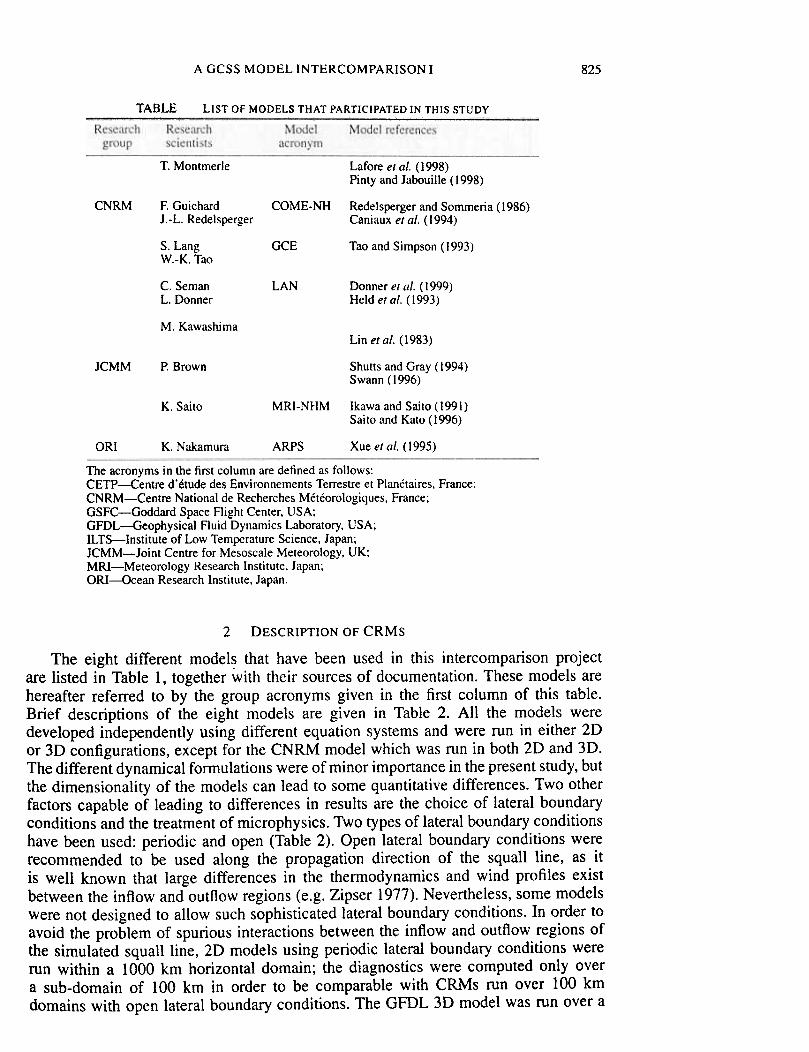
A GCSS MODEL INTERCOMPARISON I 825
TABLE LIST OF MODELS THAT PARTICIPATED IN THIS STUDY
T. Montmerle Lafore el at. (1998)Pinty and Jabouille (199:~)
CNRM F. GuichardJ.-L. Redelsperger
COME-NH Redelsperger and Somm,eria (1986)Caniaux et al. (1994)
S. LangW.-K. Tao
aCE Tao and Simpson (1993)
C. SemanL. Donner
LAN Donner et af. (1999)Held et af. (1993)
M. KawashimaLin eta/. (1983)
JCMM P. Brown Shutts and Gray ( 1994)Swann (1996)
K. Saito MRI-NHM Ikawa and Saito (1991)Saito and Kato (1996)
ORI K. Nakamura ARPS Xue et al. (1995)
The acronyms in the first column are defined as follows:CETP-Centre d'etude des Environnements Terrestre et Planetaires, France:CNRM-Centre National de Recherches Meteorologiques, France;GSFC-Goddard Space Flight Center, USA;GFDL-Geophysical Fluid Dynamics Laboratory, USA;ILTS-lnstitute of Low Temperature Science, Japan;JCMM-Joint Centre for Mesoscale Meteorology, UK;MRI-Meteorology Research Institute, Japan;ORI-Ocean Research Institute, Japan.
2 DESCRIPTION OF CRMs
The eight different models that have been used in this intercomparison projectare listed in Table 1, together with their sources of documentation. These models arehereafter referred to by the group acronyms given in the first column of this table.Brief descriptions of the eight models are given in Table 2. All the models weredeveloped independently using different equation systems and were run in either 2Dor 3D configurations, except for the CNRM model which was run in both 2D and 3D.The different dynamical formulations were of minor importance in the present study, butthe dimensionality of the models can lead to some quantitative differences. Two otherfactors capable of leading to differences in results are the choice ,of lateral boundaryconditions and the treatment of microphysics. Two types of lateral boundary conditionshave been used: periodic and open (Table 2). Open lateral boundary conditions wererecommended to be used along the propagation direction of thl~ squall line, as itis well known that large differences in the thermodynamics and wind profiles existbetween the inflow and outflow regions (e.g. Zipser 1977). Nevertheless, some modelswere not designed to allow such sophisticated lateral boundary conditions. In order toavoid the problem of spurious interactions between the inflow and outflow regions ofthe simulated squall line, 2D models using periodic lateral boundary conditions wererun within a 1000 km horizontal domain; the diagnostics were computed only overa sub-domain of 100 km in order to be comparable with CRM:; run over 100 kmdomains with open lateral boundary conditions. The GFDL 3D model was run over a

J.-L. REDEL~;PERGER et al.826
TABLE 2. KEY CHARACTERISTICS OF THE CLOUD-RESOLVING MODELS USED IN THE INTERCOMPAR.
IS,ON
No ice (2)Ice (5)
A 3D Open
CNRM 3020
Open .5 order No ice (2)Ice (5)
A
.5 order Ice (5)GSFC c-s 3D Open (x-axis)Periodic (y-axis)
order Ice (4)GFDL c. 3D Periodic
Ice (5)20 Open orderA
Ice (5)2D Periodic orderA
No ice (2)Ice (5)
c. 20 Open .5 order
No ice (2)20 Open .5 orderORI c-sThe following notation is used in column 2:A-anelastic;C-I-elastic with implicit sound waves;C-S-elastic with time splitting.
small domain with periodic lateral boundary conditions in both horizontal directions(Table 2), allowing the assessment of differences induced by the choice of lateralboundary conditions. Simulations of precipitating convective systems with trailingstratiform regions are expected to be sensil:ive to the representation of the microphysics(e.g. Yoshizaki 1986; Nicholls 1987; Chen and Cotton 1988; Tao and Simpson 1989;Caniaux et a1. 1995; Liu et ai. 1997). In the present case, the models were runwith different microphysical parametrizations both with and without an ice phase.The parametrizations represented betweelrl two and five different classes of particles(Table 2), including cloud droplets, rain dl:ops, ice crystals, aggregates, and graupel. Adetailed description of each of the eight models is not possible in the present paper but
references are given in Table 1.
3. CASE DESCRIPTION At-ID NUMERICAL EXPERIMENTS
(a) Case description and initial conditions
The general approach of this first intercomparison was to choose a case sufficientlysimple to be capable of being simulated b~1 several different models. On the other hand,the selected case needed to include sufficient physical features to be able to be comparedwith Doppler radar observations and to be: useful in the evaluation of GCM convection
and cloud parametrizations.The selected case was a 100 kilometre-long squall line observed during the TOGA-
COARE on 22 February 1993. It was well sampled by airborne Doppler radar (Fig. I)as it approached Honiara island. The two :NOAA P-3 aircraft flew for over five hours tosample the system. This case has been also chosen as a test case for intercomparisons ofdifferent radar retrieval techniques. The convective system has been extensively studiedusing both observations and CRMs by ~;everal other groups (Jorgensen et al. 1997;
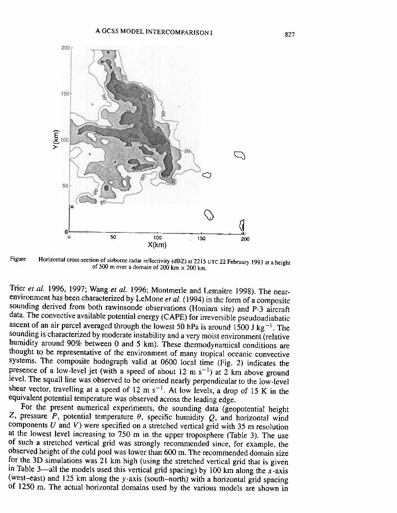
A GCSS MODEL INTERCOMPARISON I 827
~
E.x:->-
Q\0
50~
~r
-=-:;:e~"---
~ Q0
Figure Horizontal cross-section of airborne radar reflectivity (dBZ) at 2215 UTC 22 F4~bruary 1993 at a heightof 500 m over a domain of 200 km x 200 kill.
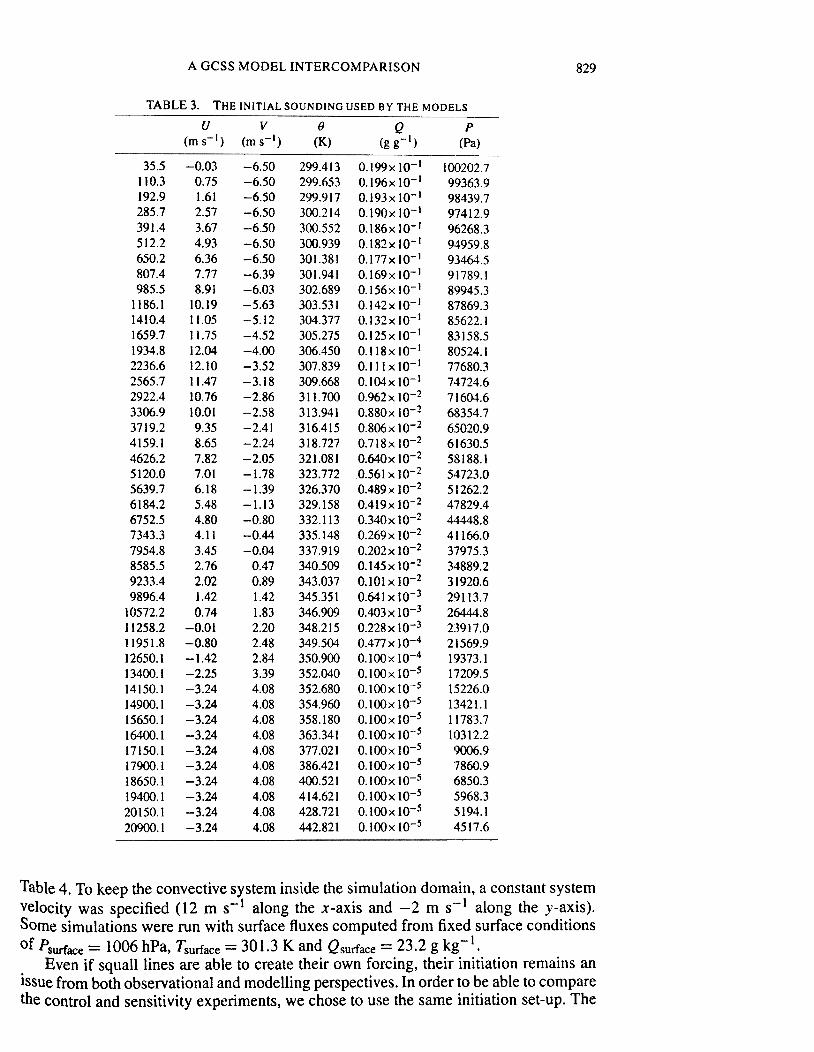
Trier et ai. 1996, 1997; Wang et ai. 1996; Montmerle and Lemaitre: 1998). The near-environment has been characterized by LeMone et ai. (1994) in the form of a compositesounding derived from both rawinsonde observations (Honiara site) and P-3 aircraftdata. The convective available potential energy (CAPE) for irreversible pseudoadiabaticascent of an air parcel averaged through the lowest 50 hPa is around 1500 J kg-I. Thesounding is characterized by moderate instability and a very moist environment (relativehumidity around 90% between 0 and 5 km). These thermodynamil:al conditions arethought to be representative of the environment of many tropical oceanic convectivesystems. The composite hodograph valid at 0600 local time (Fig" 2) indicates thepresence of a low-level jet (with a speed of about 12 m s-l) at 2 km above groundlevel. The squall line was observed to be oriented nearly perpendicul:lf to the low-levelshear vector, travelling at a speed of 12 m s -I. At low levels, a drop of 15 K in theequivalent potential temperature was observed across the leading edgc~.
For the present numerical experiments, the sounding data (ge:opotential heightZ, pressure P, potential temperature e, specific humidity Q, and horizontal windcomponents U and V) were specified on a stretched vertical grid with 35 m resolutionat the lowest level increasing to 750 m in the upper troposphere (~rable 3). The useof such a stretched vertical grid was strongly recommended since, for example, theobserved height of the cold pool was lower than 600 m. The recommended domain sizefor the 3D simulations was 21 km high (using the stretched vertical grid that is givenin Table 3-all the models used this vertical grid spacing) by 100 krn along the x-axis(west-east) and 125 km along the y-axis (south-north) with a horizontal grid spacingof 1250 m. The actual horizontal domains used by the various models are shown in
, --lA.J
50 100 150 200
X(km)

828 J.-L.. REDELSPERGER et al.
20-U)"-~
>
b
10
Figure 2. Specified initial conditions for the model runs. (a) Temperature and specific humidity plotted on askew-T log-P diagram and (b) the horizontal 1Nind components (U positive towards the east and V positive
towards the north) plotted on a hodograph---data courtesy of M. A. LeMone.
A GCSS MODEL INTERCOMPARISON 829
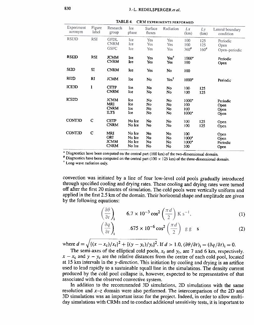
TABLE 3. THE INITIAL SOUNDING USED BY THE MODELS
U(m S-I)
V
(ms-l)()
(K)Q
(gg-l)
p(Pa)
35.5110.3192.9285.7391.4512.2650.2807.4985.5
1186.11410.41659.71934.82236.62565.72922.43306.93719.24159.14626.25120.05639.76184.26752.57343.37954.88585.59233.49896.4
10572.211258.211951.812650.113400.114150.114900.115650.116400.117150.117900.118650.119400.120150.120900.1
-0.030.751.612.573.674.93
6.367.778.91
10.1911.0511.7512.04
12.1011.4710.76
10.019.35
8.657.827.016.18
5.484.804.11
3.452.76
2.021.42
0.74-0.01-0.80-1.42-2.25
-3.24-3.24-3.24
-3.24-3.24-3.24-3.24
-3.24-3.24
-3.24
O.I99x 10-10.196x 10-10.193x 10-10.190x 10⁻¹
0.186x 10⁻¹
0.182x 10-10.177x 10-1
0.169x 10-10.156x 10-10.142x 10-10.132x 10-10.125x 10-10.118x 10-1
O.lllxIO-1O.I04x 10-10.962 x 10⁻²
0.880x 10-20.806 x 10-2
0.718x 10-20.640 x 10-20.561 x 10⁻²
0.489x 10-20.419x 10-20.340x 10-20.269 x 10-2
0.202x 10-20.145x 10-2
0.101 x 10⁻²
0.641 X 10⁻³
0.403 x 10-30.228x 10-30.477 x 10⁻⁴
O.I00x 10-40.I00xI0-5O.IOOx 10-5
O.I00x 10-5O.I00x 10-5
0.IOOxl0-5
O.IOOx 10-50.I00xI0-50.I00xI0-5O.IOOx 10-50.IOOxI0-5
O.IOOx 10-5
-6.50-6.50-6.50
-6.50-6.50
-6.50
-6.50-6.39-6.03-5.63-5.12-4.52-4.00
-3.52
-3.18-2.86-2.58-2.41-2.24-2.05-1.78-1.39
-1.13-0.80-0.44
-0.04
0.470.891.42
1.832.202.482.843.39
4.084.084.084.084.084.084.08
4.084.084.08
299.413299.653299.917300.214300.552300.939301.381301.941302.689303.531304.377305.275306.450307.839309.668311.700313.941316.415318.727321.081323.772326.370329.158332.113335.148337.919340.509343.037345.351346.909348.215349.504350.900352.040352.680354.960358.180363.341377.021386.421400.521414.621428.721442.821
100202.799363.99843'~. 7
97412.99626:g.3
9495'~.89346~.59178'~.18994:5.387869.385622.\
8315:~.58052,~.\77680.37472'~.6
7\6Q.~.66835,~. 7
65020.9
6\630.55818:~.\5472:~.05\26:2.247829.44444:~.84\16~).0
3797:5.334889.23\920.62911:~.7
2~~.82391.7.0
21569.91937:~.1
17209.51522~).013421.11178:~. 7
1031 :2.2
900~).9.7860.96850.3596:~.3519,~.1
451.7.6
Table 4. To keep the convective system inside the simulation domain, a constant systemvelocity was specified (12 m s-1 along the x-axis and -2 m s-1 along the y-axis).Some simulations were run with surface fluxes computed from fixed surface conditionsof Psurface = 1006 hPa, Tsurface = 301.3 K and Qsurface = 23.2 g kg-I.
Even if squall lines are able to create their own forcing, their initiation remains anissue from both observational and modelling perspectives. In order to Ibe able to comparethe control and sensitivity experiments, we chose to use the same initiation set-up. The
830 J .-L. REDE~LSPERGER et al.
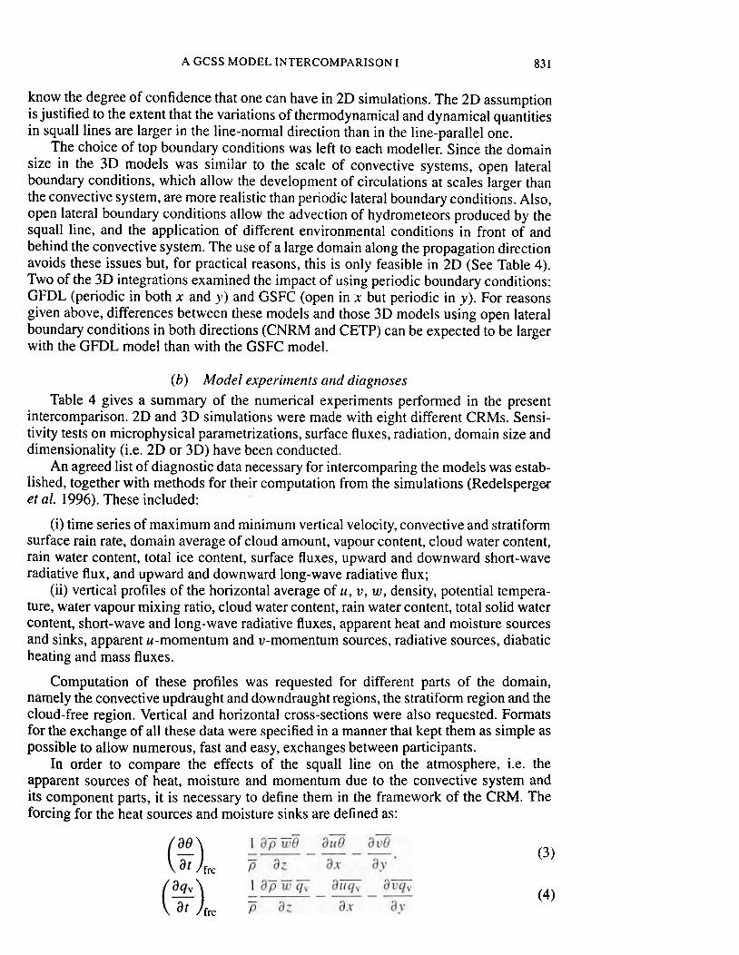
TABLE 4. CRMEXPERIMENTSPERFORMED
RSI2D RSI JCMMCNRM
YestYes
IceIce
YesYes
1000*100
PeriodicOpen
SI20 51 CNRM Ice Yes No 100
RI2D RI JCMM Ice VestNo 1000* Periodic
ICE3D I CETPCNRM
IceIce
I'iro"Ti'O
NoNo
100100
125125
ICE2D JCMMMRICNRMILTS
IceIceIceIce
N'0
N'oN'oNo
NoNoNoNo
1000*1001001000*
PeriodicOpenOpenOpen
CONT3D c CETPCNRM
No IceNo Ice
NoNo
NoNo
100100
125125
OpenOpen
CONT2D c MR!OR!JCMMCNRM
No IceNo IceNo IceNo Ice
NoNoNoNo
NoNoNoNo
1001000*1000*100
OpenOpenPeriodicOpen
* Diagnostics have been computed on the central part (100 km) of the two-dimensionsal domain.# Diagnostics have been computed on the central part (100 x 125 km) of the three-dimensional domain.t Long-wave radiation only.
convection was initiated by a line of folllr low-level cold pools gradually introducedthrough specified cooling and drying rates. These cooling and drying rates were turnedoff after the first 20 minutes of simulation. The cold pools were vertically uniform andapplied in the first 2.5 km of the domain. l~heir horizontal shape and amplitude are givenby the following equations:
6.7 x 1 O-~~ cos2 (1)
.675
x 10-6 COS2 (2)s
)i
)i
where d = J {(x -Xc)/Xr}2 + {(y ~-:;:)/~r}2. Ifd > 1.0, (ae /at)j = (aq /at)j = O.
The semi-axes of the elliptical cold p,ools, Xr and Yr, are 7 and 6 kIn, respectively.x -Xc and Y -Yc are the relative distanc:es from the centre of each cold pool, locatedat 15 km intervals in the y-direction. This initiation by cooling and drying is an artificeused to lead rapidly to a sustainable squall line in the simulations. The density currentproduced by the cold pool collapse is, hl~wever, expected to be representative of thatassociated with the observed convective s:ystem.
In addition to the recommended 30 simulations, 20 simulations with the sameresolution and x-z domain were also pe:rformed. The intercomparison of the 20 and30 simulations was an important issue fair the project. Indeed, in order to allow multi-day simulations with CRMs and to condul:;t additional sensitivity tests, it is important to
A GCSS MODEL INTERCOMPARISON I 831
know the degree of confidence that one can have in 2D simulations. The 2D assumptionis justified to the extent that the variations of thermodynamical and dynamical quantitiesin squall lines are larger in the line-normal direction than in the lint~-parallel one.
The choice of top boundary conditions was left to each modeller. Since the domainsize in the 3D models was similar to the scale of convective systems, open lateralboundary conditions, which allow the development of circulations at scales larger thanthe convective system, are more realistic than periodic lateral boundary conditions. Also,open lateral boundary conditions allow the advection of hydrometeors produced by thesquall line, and the application of different environmental conditions in front of andbehind the convective system. The use of a large domain along the propagation directionavoids these issues but, for practical reasons, this is only feasible in 2D (See Table 4).Two of the 3D integrations examined the impact of using periodic boundary conditions:GFDL (periodic in both x and y) and GSFC (open in x but periodic in y). For reasonsgiven above, differences between these models and those 3D models using open lateralboundary conditions in both directions (CNRM and CETP) can be t~xpected to be largerwith the GFDL model than with the GSFC model.
(b) Model experiments and diagnoses
Table 4 gives a summary of the numerical experiments perfonned in the presentintercomparison. 2D and 3D simulations were made with eight different CRMs. Sensi-tivity tests on microphysical parametrizations, surface fluxes, radiation, domain size anddimensionality (i.e. 2D or 3D) have been conducted.
An agreed list of diagnostic data necessary for intercomparing the models was estab-lished, together with methods for their computation from the simulations (Redelspergeret al. 1996). These included:
(i) time series of maximum and minimum vertical velocity, convl~ctive and stratiformsurface rain rate, domain average of cloud amount, vapour content, c::loud water content,rain water content, total ice content, surface fluxes, upward and downward short-waveradiative flux, and upward and downward long-wave radiative flux;
(ii) vertical profiles of the horizontal average of u, v, w, density, potential tempera-ture, water vapour mixing ratio, cloud water content, rain water contlent, total solid watercontent, short-wave and long-wave radiative fluxes, apparent heat and moisture sourcesand sinks, apparent u-momentum and v-momentum sources, radiatilve sources, diabaticheating and mass fluxes.
Computation of these profiles was requested for different parts of the domain,namely the convective updraught and downdraught regions, the stratiform region and thecloud-free region. Vertical and horizontal cross-sections were also requested. Formatsfor the exchange of all these data were specified in a manner that kept them as simple aspossible to allow numerous, fast and easy, exchanges between partil::ipants.
In order to compare the effects of the squall line on the 2ltmosphere, i.e. theapparent sources of heat, moisture and momentum due to the convective system andits component parts, it is necessary to define them in the framewo]~k of the CRM. Theforcing for the heat sources and moisture sinks are defined as:
(3)
(4)
)fOC
)frC

832 J.-L. REDELS,PERGER et al.
where e is the potential temperature, qy the mixing ratio of water vapour, and p thedensity. The overbar denotes a horizontal a'/erage of the variable over the domain and atime average over I hour. The apparent heat source Q lC and moisture sink Q2 for thetotal domain are then defined as: .
aeat
a()
)at frcQR QR'7T
aqv
at
aqv
)~ frc (6)
(7)
where 7f = (T I(J) = (pi PO)R/Cp and QR is the radiative term.There is no general agreement about the best way to separate stratiform and con-
vective columns. The present study uses a method similar to that of Tao et at. (1993).A cloudy grid box is defined as one in which the mixing ratio for total hydrometeorsexceeds 5 x 10⁻⁶ g g-i. A first simple criterion for the convective/stratiform separationis that any vertical column with a surface rain rate ~ 20 mm h -I is considered as convec-
tive. In addition, vertical columns for which the surface rain rate exceeds ~ 4 mm h-1and is twice as large as the average taken over the 24 surrounding grid points in the 30models (4 in the 20 models) are identified as the cores of convective cells. For eachsuch core column, the 8 surrounding columns in 30 (2 in 20) are also considered asconvective columns. Cloudy columns not c:lassified as convective are considered to bestratiform.
Similarly, it is possible to define an arlparent momentum source, representing theeffects of unresolved convective circulations on the mesoscale momentum field. Thelarge-scale forcing for u- and v-momentum is defined as:
'~ ) =-~~~ __pauu --
,at frc aZ
'apv ) apWV-, at -frc = -az ax -ay- ay .,,-,
The apparent sources of u-momentum ,md v-momentum are then defined as:
_auv ap--p---
ax ay ax
aliV a"ij""V" ap--p -- (8)--p
apuat
(apu
),-ar- frcQu (9)
apvat
apv)at frcQv
The eight SCMs have also been run with the same initial conditions and withimposed large-scale tendencies of temperature and moisture (Eqs. (3) and (4)) deducedfrom experiments with an open-boundary CRM (Redelsperger et al. 1996). Results fromthese SCMs are reported in a companion pclper (Bechtold et al. 1999).
It is worth noting that the forcing tefitS specified by Eqs. (3), (4), (7) and (8) areidentically zero for CRMs running with periodic lateral boundary conditions whencomputed on the ful1 simulation domain. Indeed, the horizontal average of w overthe domain is equal to zero in this case, £lS wel1 the horizontal average of horizontalgradients. Consequently, when it was possible, and as noted in Table 4, the computationsof these quantities were made over a sub-domain of a size identical to that of therecommended domain in the intercomparison (i.e. 100 km in the x-direction).

A GCSS MODEL INTERCOMPARISON 833
--C_2D_CNRM ---1_2D_CNRM-* C_2D_MRI -*- -1_2D_MRI-+- RSI_2D_JCMM -* C_2D_ORI
.SI_2D_CNRM
-$- -1_2D_.JCMM-6- C_2D_ILTS
-RSI_2D_C"IRM$-- RI_2D_JC"'IM6- 1_2D_ILTS a30
';j;"
g?:-"g""(i;>
~tQ)>
.10
0 50 100 150 200 250
Simulation time (min)300 350 400
--C_3D_CNRM ---'_3D_CNRM ~'RSI_3D_CNRM -¥- RS'_3D_GSIFC -0 C_3D_CET
-H- RSI_3D_GFDL -E!) -'_3D_CETP,., " I'Ib' .I I , -1-'
I ';, J~, I .
I' I
\t.-
30 ~@Y I , I!JI J ' .I ,I "'/ /I I, '"/,,
,." II , I'I I I\,}...
,,, (j,II " \
I
ii!:-"S""(i;>
~.1;:Q)>
-~; ,., ..,), ',
l'f-'
J~4/\
"'"'r~" ,
~~~ /~~'~J\\ ~ -f!:5 -~.
I .t
,C!! -(!S i!>~)
\(;., --.",.
10
.-200 250
Simulation time (min)0 50 100 150 300 360 400
Figure 3. Time history of the maximum and minimum vertical velocity (m s-l) for (a) the 2D cloud-resolvingmodels, and (b) the 3D cloud-resolving models (see Tables 1 and 4 for an explanation of the acronyms).
4, RESULTS
Overall, both 2D and 3D models were able to simulate a number of qualitative fea-tures of the squall line. These include a leading convective region with large precipita-tion rate, a stratiform region of reduced precipitation rates, a large !iystem propagationspeed and a warming and drying of the atmosphere. The comparison of some fieldsdid, however, show significant quantitative differences. In this paper, it is possible topresent only a small amount of data gathered during the intercomparison project. Theinterested reader can also find a comprehensive collection of the re:;ults on the WWWpage dedicated to this case (URL: http://www.cnrm.meteo.fr/gcss/).
(a) Time series
Figure 3 shows the time history of the maximum and minimum vertical velocitiesfor the 2D and 3D simulations. Each class of experiments generates. a family of curveswith general agreement between all models. The spin-up time of the: convection for thetriggering used is roughly the same for each model except GFDL. The 3D experiments
20-
10
0
20
10
0

834 J .-L. REDE~LSPERGER et al.
exhibit generally more variations betwl~en them than the 2D experiments. The 2Dexperiments produce significantly smallc~r values (half the magnitude) compared withthe 3D experiments. For both the 2D and the 3D experiments, the downdraught valuesare approximately half the updraught on(~s, a result also true for the mean values in theconvective region. The total surface rain rate (Fig. 4) exhibits larger differences fromexperiment to experiment for an individual model, and from model to model for thesame experiment. Nevertheless, independently of the type of experiment, the resultsstay in the same general range of values apart from the GFDL 3D model using periodiclateral boundary conditions in both horizontal directions. The lower precipitation rates,but similar vertical velocity extrema, of the GFDL model during the later part of thesimulation suggest that it has a reduced area fraction of convective cells in comparisonwith the other 3D models. The 2D results are generally close to those of the 3D modelsexcept for the two first hours.
It is important to note that in the present simulations, the models are not constrainedby an imposed large-scale forcing. We are~ looking at an initial value problem where thesimulated convective systems formed thc~ir own large-scale forcing. Fast-propagatingsquall lines are considered to be self-forced systems creating their own convergencezones and large-scale ascent. The main input from large scales for such systems is theconvective available potential energy. Keeping in mind these considerations and lookingat 3D results for the total surface rain (Fig. 4), there is quite good agreement betweensimulations using ice-phase microphysic1; and open lateral boundary conditions alongthe direction of system propagation (CNRM, CETP and GSFC). The inclusion of anice parametrization results in a small increase in precipitation for both 2D and 3Dexperiments. Experiments taking into account surface fluxes and/or radiative processeslead to a slight increase in precipitation. Another feature also apparent in the timeevolution of the rainfall (Fig. 4), is that the 20 experiments show more temporalvariations on scales of 20-100 min than the 3D experiments. Surface rain rates werefurther partitioned into stratiform and con'rective parts, which are important to know forSCMs (see Bechtold et al. 1999). The time history of the stratiform rain rate (Fig. 5)again shows general agreement between thle 3D models except for the GFDL model. Onaverage 70% of the total rain rate is convective and 30% stratiform. This partitioningwas found by shipbome radar to be common for systems observed during disturbedperiods of the TOGA-COARE (Short et at. 1997).
From both Figs. 4(c) and 5(c), it is clear that the main problem in the GFOLsimulation stems from an insufficiently developed stratiform region. One possible reasonis the use of a small domain (100 km) with periodic lateral boundary conditionsin both horizontal directions. In contrast" the GSFC 3D model with periodic lateralboundary conditions in only one direction produces similar stratiform precipitation andslightly less convective precipitation than tlhe other 3D models with fully open boundaryconditions (CNRM and CETP). Opening the boundary conditions in the propagationdirection has, therefore, a large impact. In the GFOL simulation with full periodic lateralboundary conditions, non-zero domain-averaged vertical motions cannot develop. Sincethe domain size in this simulation is not much larger than the system itself, this precludesthe development of a larger-scale circulation which can intensify the convective systemthrough positive feedback. This behaviour differs from the 3D simulations with openboundary conditions in the propagation direction (CNRM, CETP and GSFC), whichdevelop domain-averaged vertical motions, as discussed later. The domain-averagedvertical motions in the latter simulations, \),.'ith their vertical velocity peaks in the middleand upper troposphere, generate convective instability. In addition the use <:>f periodiclateral boundary conditions along the prop:agation direction on a small domaIn Imposes

A GCSS MODEL INTERCOMPARISON 835
---1_3D_CNAM ~ ASI_3D_CNAM
-¥- ASI_3D_GSFC ~ ASI_3D_GFDL
-E!) -1_3D_CETP
201(;
15
~---~
.,
-:;::co
~g.s 1~
~--~-
~5~~
o~0 50 100 150 200 250
Simulation time (min)
5
~~
~
I
400300 350
Figure 4. Time history of the tota.l surface rain rate (cm day-I) for (a) the 20 and 30 cloud-resolving models(CRMs) with no ice-phase parametrization, (b) the 20 CRMs with an ice-phase paramel:rization, and (c) the 30
CRMs with an ice-phase parametrization (see Tables I and 4 for an explanation of the acronyms).
o~

836 J .-L. REDIiLSPERGER el al.
10 1_2D_CNRM .SI_2D_CNRI~-RSI_2D_CNRM -~- -1_2D_MRI-<>- -1_2D_.JCMM --~-- RI_2D_.JCMlo1~ RSI_2D_.JCMM -.b- -1_2D_IL TS
8 f\ :~'"f\J l¥V:,., ~ "
,it> I,'I
" I III ~I, "I I'
~ '.~\ \:.~) I
1"-'\\
~~ 6.£co.~
~ 4~U5
)~,. , I, ,{
r-)\
\/ / II
I ..'t
;-4 I ,,' , ,,'J' V", I I \ I, , \ .:..." ,., '"( i" -..'",. ,,;I!>-,I, \, ...I AI , , :1I' ,\ .,,~ ' ,
,', ~,' ,\.,!:' 1\ -' ""t I .\~(-
~~
/\Y"A \II ~\ .
2 , ,\t,~ \/
..-.-350r--~I ;J": ~ '. I0
50 100
~~~~~~~
E)-; ~~~~~~:='" --'./""- -'-- ~ --,- ~..,. ..
--cZJ- ---~ ---.~,~~~~~~~~:~~:~: ~~ -E)': --
0 50 100 150 200 250Slml.llatlon time (mln)
2
0
300 350 400
As Fig. 4, but for the stratifonn surface rain rate (cm day-l ).Figure 5.
,., ' V " ,1"" '-I I" \ \
!'.,. \
O-j I I --I
150 200 250 300 400
Simulation time (min)
1 -~ -1_3D_CNRM ~ RSI_3D_CNR'-I1
C-¥-- SI_3D_GSFC ~ RSI_3D_GFDL
-E!) -1_3D_CETP
">;(0
~~c:.~E,g 4"§U5

A GCSS MODEL INTERCOMPARISON 837
the same atmospheric characteristics both in front of and behind the convective system.Thus, the 3D convective system with periodic lateral boundary conditions generatesconsiderably less precipitation. Figures 4(c) and 5(c) imply that precipitation from boththe convective and the stratiform regions in the GFDL simulation is le:ss than in the other3D simulations. With less generation of convective instability possibl(~ in this simulation,the convective circulations are less developed. There is, in turn, less condensate availableto feed the stratiform component of the system.
Confirming these points, the JCMM experiments using a large 20 domain (1000 km)together with periodic lateral boundary conditions are able to produce large stratiformregions. In the 20 experiments, differences in the partitioning betw(~en convective andstratiform regions come from differences in the microphysical schemes. For example,lower terminal fall speeds of ice hydrometeors generally correspond to a reducedstratiform region as they allow for the hydrometeors formed in the convective region tobe advected farther to the rear of the system. As seen in Fig. 5(b), the: JCMM 2D modelwith an ice phase produces larger amounts of stratiform rainfall than other models.Further tests with this model have shown that this discrepancy is reduced \Jv'hen themean fall-speed of cloud ice is increased.
Comparisons of the time evolution of domain-averaged liquidl and solid (whenpresent) water content (Fig. 6) indicate a generally good agreement, except (and forthe same reasons as above) for the GFOL experiment with periodic lateral boundaryconditions, and for the three 2D experiments produced from the JC~1M model. Again,tests with the JCMM model have shown that this discrepancy is reduced when the meanfall-speed of cloud ice is increased. Apart from these differences, the agreement is quitenoticeable and encouraging. In particular, it is important to note that the 20 and 3Dmodels have similar quantitative behaviours. Also, the ice phase does not seem to beimportant for predicting the domain-averaged total water content. This is to be expectedsince the 4 km depth between cloud base and the freezing level mearlS that much of therain will be formed by coalescence/collection even in those models with an ice phase,and experiments without an ice phase can produce liquid water abo.v(~ the O°C isothermlevel. Of course, we should still expect differences in the vertical distributions of the
hydrometeors.
(b) Three-dimensional stnlcture
Examination of horizontal cross-sections of the simulations at different times indi-cates that the 3D experiments are able to reproduce to some extent the different stages ofthe observed system as it develops from the linear-configuration stage to the bow-shapedstage (Fig. 7). As observed by airborne radar (Fig. 1), the convective region formed atthe leading edge of the system which was moving to the east (on the right in the figures),corresponding to strong convective updraughts and downdraughts (F;ig. 8). Behind theconvective region, an extended stratiform region is simulated with le:ss intense v'erticalmotions and lower water contents. More detailed comparisons show that the 3D modelsare also able to simulate the observed mesoscale horizontal vortice~; occurring on thenorthern and southern parts of the system (Trier et al. 1997; Montmerle et al. (personalcommunication». Nevertheless, the comparison of horizontal cross-sections shows thatthere are some qualitative and quantitative differences between experiments after 6 h ofsimulation. Again, the use of periodic lateral boundary conditions on a relatively smalldomain (GFDL) decreases the intensity of the system and leads to a less developedstratiform region (Figs. 7(b) and 8(b». On the other hand, the values of vertical velocityand total water content agree quite well for the three other experiments (CETP, CNRMand GSFC). As confirmed by the time series of vertical velocity exltrema (Fig. 3), the

838 J .-L. REDI~LSPERGER et al.
0.3 --C_2D_CNRM --C_2D_MRI-*- C_2D_ORI -A- C_2D_IL TS--C_3D_CNRM -e- C_3D_CETI>
0.25
~EQ)E8!!!0Q)
Q;Ee-g..-="Cij-0I-
0.2
0.15
~~~-~0.1 ~
-
0.05J", ~ ~ ~
.-:::~=====:::=~---0.0
-I I I I I
200 250 300 350 400Sllmulatlon time (min)
0 50 100 150
0.3 '_20_CNRM .SI_20_CNRM---RSI_2D_CNRM -~- -1_20_MRI-~ -1_20_JCMM -.~.- RI_20_JCIIAM-e.- RSI_20_JCMM -b -1_20_IL TS
F ~-- '-':-.::-_&_-,~ ,-' -~ ~ -)( --' ,- -' , -,.-
,,',.
'->E'--,-A ,,
, -
.-A-,
~-/~/ 0:::- _8- --/ "..-0.05 ~ -
--,,-& "--~-- I ," ~-- ~--~-I I I I I
0 50 100 150 200 250 300 350 400Sirnulation time (min)
0.0
-.-1_3D_CNRM -RSI_3D_CNRM-¥- RSI_3D_GSFC -'H- RSI_3D_GFDL
-e>- 1_3D_CETP
0.:3
c
-e- --~
--?-~-.,v:..:::.-,"-=-~..G---::;~~~..",. -.- "
---~~ ~~~ H-~-"" ..,~~:::::=~==::; ~, I I I I
0 50 100 150 200 250 300 350 400Simulation time (min)
0.05
0.0
As Fig. 4, but for the domain-averaged total hydromet.eor (liquid + solid) water content (g m-3).Figure 6.

A GCSS MODEL INTERCOMPARISON 839
2 'ig
Figure 7. Horizontal cross-sections of the total hydrometeor fields (contour interval 1.0 g kg-I, except that thefirst two isolines correspond to values of 0.1 and 0.5 g kg-I) after 6 hours run time and at a height of 1.4 kIn forruns (a) I3D (CETP), (b) RSI3D (GFDL), (c) RSI3D (GSFC), and (d) RSI3D (CNRM) (st:e Tables I and 4 for an
explanation of the acronyms).
vertical velocity amplitudes in the convective cores are similar for all four 3D experi-ments, and their horizontal sizes are also similar. The reduction in the fractional area ofthe convective cells in the GFDL model, which was suggested above, is readily apparentin Fig. 8(b).
Vertical cross-sections of radar reflectivity and vertical velocity derived from twodifferent analyses of airborne Doppler radar (Jorgensen et al. 1991'; Montmerle and
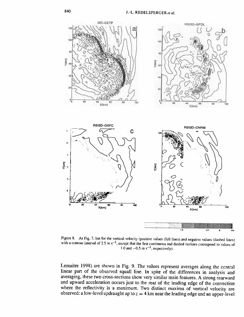
840 J.-L. REDELSPERGER el al.
120
100100
8080
~>80
E I.¥):'60
4"40
f)
20201/
/' I
-=-~;
/ /L
'0
20 '0 80 80 100 0 20 40 80 100X(km)X(km)
15 45 6 "".Figure 8. As Fig. 7, but for the vertical velocity (positive values (full lines) and negative values (dashed lines)
with a contour interval of 2.5 m s-I, except that the first continuous and dashed isolines correspond to values of
1.0 and -0.5 nrl s-I, respectively).
Lemaitre 1998) are shown in Fig. 9. Thl~ values represent averages along the centrallinear part of the observed squall line. In spite of the differences in analysis andaveraging, these two cross-sections show very similar main features. A strong rearwardand upward acceleration occurs just to the rear of the leading edge of the convectionwhere the reflectivity is a maximum. Two distinct maxima of vertical velocity areobserved: a low-level updraught up to z = 4 km near the leading edge and an upper-level

A GCSS MODEL INTERCOMPARISON 841
18.1 -:
18'rf
J 'E1,~~ N~
"a1
c-;i;~' ~;/~ ;...,~\Iv .~:;;;~2
~~V ~ ~\ 4 \\: I ,\ ~D8' \ /- \ '-'1\ \ ~\ ~\\J\5\\i
I \ \ '\"- \ \ \.
t >~.
~~-2
C~ [:=:::: "--"'L--' N
~,'--~~::-=--", ,-.:~\", ~
r rr;, ..~\ \!'""""",\'" " " \:~, ~\:~\ "
\..,..,,\\', :,',\\\"...'.',", ')\ \\\'
0, L~_~~:=-.::j; I "'- \ U" .' I 0 ~ ',\, 4-J Z
".~ \. / --_0 A" \,"'zVII 0 .I I '. ',~/I~.
,
57. O. 57.
o.o.
15.
L
b-
d-..E~--N -", I
~r\ .
.~.
...::~
.'. .,..T:~..'.' X(km)
!y
2C",, .'
o. _-.:_-o. ::~~:o.
-
57. o.-
57
Figure 9. Vertical cross-sections (a) and (b) of radar reflectivity (dBZ. contour interval 5 dBZ). and (c) and (d)of vertical velocity (m s-l. contour interval I m s-l) as analysed from Doppler radar observations around 2100UTC 22 February 1993 over domains (a) and (c) 57 kIn x 18 kIn constructed from 40 kIn averages along the squallline (Jorgensen et al. 1997). and (b) and (d) 57 kIn x 15 kIn constructed from 7 km aver;lges along the squall line
(Montmerle and Lemaitre 1998). Doppler wind arrows are shown in (a).
updraught from z = 5 to 15 km, 15-20 km to the rear. Another notic:eable feature is thepresence of weak mean downward motions at the rear of the system. The differences inthe position and amplitude of the downward motions as deduced from the two methods,and the two different line-averages, can be explained to a large degrt~e by the variabilityalong the squall line, as illustrated by Fig. 8 and discussed by Jorgensen et ai. (1997)and Trier et ai. (1996). Detailed examination of the observed fields rc~veals that the mid-tropospheric vertical-velocity minimum is a common, but not persi~;tent, feature of thecentral linear part of the squall line.
Figures 10 and 11 indicate that all the 20 and 30 simulations produce a strongmaximum of total water content and vertical velocity in the convective region, asobserved (Fig. 9). A rather good agreement is found between tile simulated fieldsfrom the 3D models with open lateral boundary conditions in the prc)pagation direction(CETP, CNRM and GSFC) (Figs. 10(g), (h) and (i» and the observ~~d fields of verticalvelocity. In particular, the tilting of the updraught region, the altitudes of the low-level and upper-level maxima, and their horizontal separations closely resemble those

842 J.-L. REDELSPERGERetal.
C2D-ORI/'
12D-JCMM
,.~~
1
,0-
,.~IiA
\~' , ~
I'\.
-.J\
10~EN
E ~. v 0'" '.. 1
:~:. ..eo20
X(km)
12D-ILTS
d
Figure 10. Vertical cross-sections of the vertical velocity (ms- t, contour interval I m s-l) after 6 hours run timefor runs (a) C2D (ORI), (b) I2D (JCMM), (c) 12D (MRI), (d) I2D (ILTS), (e) I2D (CNRM), (f) RSI3D (GFDL),(g) RSI3D (CNRM), (h) RSI3D (GSFC), and (i) I3D I:CETP)-only part of the simulation domain is shown (see
Tables I and 4 for an e~,planation of the acronyms).
observed. The GFDL 3D model with lateral periodic boundary conditions is able toreproduce some of these features, though with a larger tilting of the updraught regionand less intense motions (Fig. 10(f». The vertical development behind the leadingconvective region predicted by the 2D CR.Ms shows some differences from experimentto experiment. These differences occur in both the vertical velocity and the total watercontent fields (Figs. 10(a)-(e) and 1 I (a)-(e» and seem to arise mainly from differencesin the microphysical parametrizations. Nevertheless, most of the models which includean ice-phase parametrization are able to ~;imulate the double-maxima vertical-velocitystructure as observed by Doppler radar (iFig. 9) although the (.\", z) locations of thesemaxima differ. The comparison for the 2D experiments is difficult for many reasons.For example, owing to a strong rearward flow, the JCMM and ILTS experiments producetheir secondary updraught maxima in the Imid-to-upper troposphere more than 50 km tothe rear of the leading edge of the squalllil1e and cannot, therefore, be seen in the figure.It is also important to stress the difficulties in the comparison of such fields owing tothe large space and time variations in cow/ective activity. The 2D simulations generallyexhibit more time variability than the 3D simulations. One explanation is that the flowin the 2D models is constrained in the )C-z plane and lacks the observed variabilityalong the line. Comparisons between the 2D and 3D experiments performed with thesame model (CNRM) show that the spatiaJ variability in the 3D run is replaced by timevariability which is reinforced in the 2D run (not shown). This is partly illustrated bythe vertical velocity field of these two experiments (Figs. 10(e) and (g». In the 2Dexperiment a succession of updraughts and downdraughts is seen, contrasting with thecontinous region of vertical velocity in th(~ 3D run.

A GCSS MODEL INTERCOMPARISON I 843
RSI3D-C3FDL
) /" f
0 15 3. 4.5 E nVs
Figure 10. Continued.
Other comparisons (not shown) between the observations and 'the 3D simulationshave been made for thermodynamic parameters. The 3D experimen1:s are able to repro-duce the amplitude and structure of the large decrease in moist static energy caused bythe decrease in humidity. This feature is less well represented in tlle 2D experiments.One reason is that the 3D experiments have stronger updraughts and produce strongerconvection-induced downdraughts causing larger drying in the cloudl-free area.
I
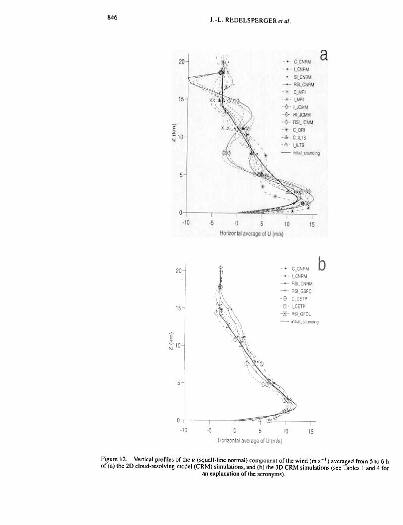
(c) Vertical profilesExamination of the wind profiles from the 3D simulations indicates that the av-
erage effect of the convective system is to decrease the intensity of the low-level jet(Fig. 12(b». All the 3D experiments that include the ice phase also produce an increaseof the line-normal wind between 9 and 16 km related to upward mlotions observed inthese experiments in Figs. IO(g), (h) and (i). The amplitudes of these <:hanges in the windare considerably less (about 5 times) than those found in previous studies of Africansquall lines observed during the COPT81 experiment (Caniaux et £j~l. 1995). The line-parallel wind is also slightly decreased in low levels in experiment~. CETP and GFDL(Fig. 13). In contrast to the other 3D models. the CETP 3D exoeriments with and without
844 J .-L. REDEI_SPERGER et al.
C2D-QRI120-JCMM
ba '"
[00
! !
"'-.
:...J
12D-MRI
Figure 11 As Fig. 10, but for the total hydrometeor (liquid + solid) fields (g kg-I. contour interval 1.0 g kg-texcept that the first two isolines correspond to values of 0.1 and 0.5 g kg-I ).
an ice phase predict an increase of line-normal wind in the boundary layer. This featureis not observed and needs to be understood in the future.
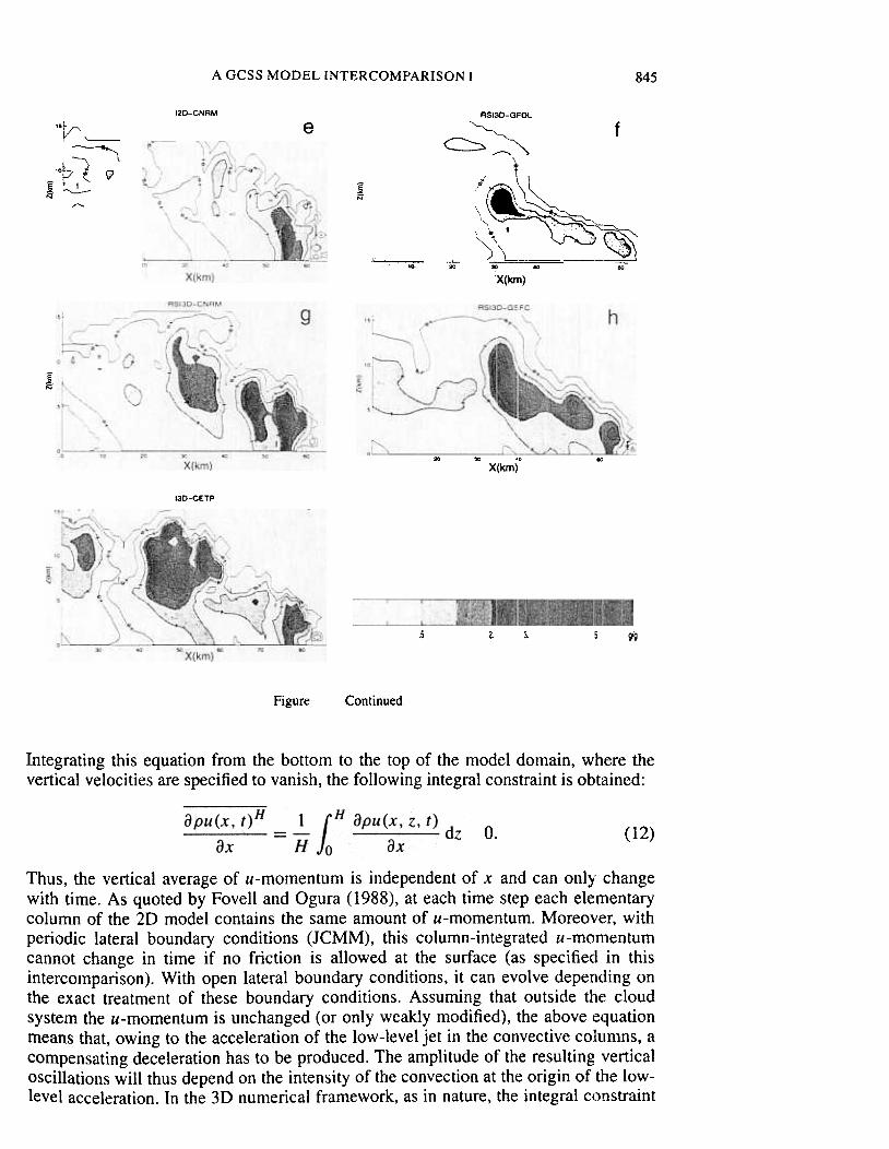
All the 2D experiments exhibit an acceleration of the low-level jet which is absentin all 3D experiments (Fig. 12(a)). Above the jet, the 2D models also show verticaloscillations in the line-normal wind. The amplitude of acceleration and oscillationsdepends on models and convection inte:nsity. More active convection induces largeramplitudes of acceleration and oscillations. Thus, the JCMM 2D experiments thatproduce more hydrometeors (Fig. 6) anlj rainfall (Fig. 4) than other 2D models havethe largest oscillations. The 2D experiments with no ice phase (less active) have thesmallest oscillations. The different beha'viour of line-normal wind, as predicted by the2D and 3D models, can be analysed as foJlow. Horizontal cross-sections of the simulatedsquall lines (Figs. 7 and 8) clearly display the three-dimensional character of the flow,both at the convective-cell scale and the system scale. In particular, the structure of thehorizontal flow (not shown) shows an asymmetric structure over a significant part ofthe system, with a tendency to form vortices at the northern and southern parts of thesquall line. These features were clearly observed in the northern part by Doppler radars(Jorgensen et al. 1997). The central part exhibits flow acceleration relative to the otherparts. The northern and southern parts of the system have an orientation which differsfrom the low-level environmental shear, and the momentum transports consequentlydiffer. To a first approximation, the flow structure in the central part of the squall line isquasi-2D and, in this limited part of the ~;ystem, the 3D simulations produce an increasein the line-normal shear which is well reproduced by the 2D simulations. The originof vertical oscillations in the 2D simulations can then be explained by considering theanelastic continuity equation in a 2D framework:
1
A GCSS MODEL INTERCOMPARISON I 845
12D-CNRM RSI3D-GFDL
~c:::::::::.~~
fe
"V'
' =:-~
-'O
~.5 I
N "'"
9
~
(I\ ~~~~;~}~\ ~" ' ~ t , c;,
)"\ --
~N
---=
~ 40
X(knl)
,. ,, o. .. 80
IN
20 ~ '0
X(km)eo
130-CETP
.5 2 3 5 '19
Figure Continued.
Integrating this equation from the bottom to the top of the model t:lomain, where thevertical velocities are specified to vanish, the following integral constraint is obtained:
o. (12)
Thus, the vertical average of u-momentum is independent of x and can only changewith time. As quoted by Fovell and Ogura (1988), at each time step each elementarycolumn of the 2D model contains the same amount of u-momentum. Moreover, withperiodic lateral boundary conditions (JCMM), this column-integrated u-momentumcannot change in time if no friction is allowed at the surface (as specifiect in thisintercomparison). With open lateral boundary conditions, it can evolve depending onthe exact treatment of these boundary conditions. Assuming that outside the cloudsystem the u-momentum is unchanged (or only weakly modified), 1the above equationmeans that, owing to the acceleration of the low-level jet in the convective columns, acompensating deceleration has to be produced. The amplitude of the resulting verticaloscillations will thus depend on the intensity of the convection at th(~ origin of the low-level acceleration. In the 3D numerical framework, as in nature, the integral constraint
846 J.-L. REDELSPERGERetal.
Figure 12. Vertical profiles of the u (squall-line normal) compont:nt of the wind (m s-l) averaged from 5 to 6 hof (a) the 20 cloud-resolving model (CRM) simulations, and (b) the 3D CRM simulations (see Tables I and 4 for
an explanation of the acronyms).
A GCSS MODEL INTERCOMPARISON 847
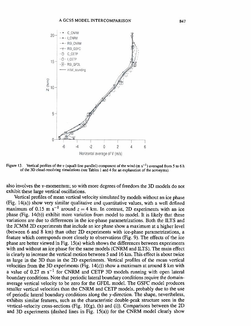
Figure 13. Vertical profiles of the v (squall-line parallel) component of the wind (m s-l) averaged from 5 to 6 hof the 3D cloud-resolving simulations (see Tables I and 4 for an explanation of the acronyms)"
also involves the v-momentum; so with more degrees of freedom the 3D models do notexhibit these large vertical oscillations.
Vertical profiles of mean vertical velocity simulated by models without an ice phase(Fig. 14(a)) show very similar qualitative and quantitative values, with a well definedmaximum of 0.15 m s-1 around z = 4 km. In contrast, 2D experiments with an icephase (Fig. 14(b)) exhibit more variation from model to model. It is likely that thesevariations are due to differences in the ice-phase parametrizations. Both the ILl'S andthe JCMM 2D experiments that include an ice phase show a maximuJm at a higher level(between 6 and 8 km) than other 2D experiments with ice-phase parametrizations, afeature which corresponds more closely to observations (Fig. 9). Th(~ effects of the icephase are better viewed in Fig. 15(a) which shows the differences between experimentswith and without an ice phase for the same models (CNRM and ILTS.). The main effectis clearly to increase the vertical motion between 5 and 16 km. This effect is about twiceas large in the 3D than in the 2D experiments. Vertical profiles of the mean verticalvelocities from the 3D experiments (Fig. 14(c)) show a maximum at around 8 km witha value of 0.27 m s-1 for CNRM and CETP 3D models running with open lateralboundary conditions. Note that periodic lateral boundary conditions r(~quire the domain-average vertical velocity to be zero for the GFDL model. The GSFC model producessmaller vertical velocities than the CNRM and CETP models, probably due to the useof periodic lateral boundary conditions along the y-direction. The shape, nevertheless,exhibits similar features, such as the characteristic double-peak stnlcture seen in thevertical-velocity cross-sections (Fig. 10(g), (h) and (i)). Comparisons between the 2Dand 3D experiments (dashed lines in Fig. 15(a)) for the CNRM model clearly' show
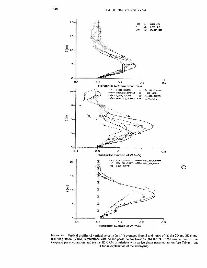
848 J.-L. RI~DI~LSPERGER,etal.
20--CNRM_2[) -MRI_2D-oijE- ORI_2D -6- IL TS_2D
CNRM_3[) -~ -CETP _3D
~15
~-;::;10
5
0
-,
0.3-0.1 0.0 0.1 0'.2Horizontal average of W (m/s:~
; 1_21:1_CNAM .SI_2D_CNAM--~ ASI 2D CNAM --~ -, 2D MAl
:;:. -~ -'_2C;_JCMM ---0-- RI_2D_JCMM..,0 --~',- 0 ~ ASI__2D_JCMM -,~- 1_2D_ILTS
, 0 0.,
20
15 x.
~N 10
,,- -.': -',
"x 6'~:';~~~,' -', '. "':'-""~;.;: :~-
',--',-. ---' ~, ". ' .x .'." ~,~,
---',' ,,:.:;y.i, ;;:-:::;':':;'Co. :- : -' ~~ :=::00.1
0.0 0.1 0.2Horizontal average of W (m/s)
'_3D_CNRM -RSI_3D_CNRM-¥- RSI_.3D_GSFC -"H:-. RSI_3D_GFDL-E!)- 1_3D_CETP
::J>
5
0
-I
I
0.3
,l~I" I
" I" ,
20
c15
~N 10 '~, ---
5
0
-0.1
~"",~~~;;;J- ~ -,
/ -~k~~~.,1g ---:;.-~ -r -;;,-- --:-
I ...
:--
~ I I
0.0 0.11 0.2 0.3Horizontal averclge of W (m/s)
Figure 14. Vertical profiles of vertical velocity (m s--I) averaged from 5 to 6 hours of (a) the 2D and 3D cloud-resolving model (CRM) simulations with no ice-pha.se parametrizaltion, (b) the 2D CRM simulations with anice-phase parametrization, and (c) the 3D CRM simulations with an ice-phase parametrization (see Tables I and
4 for an explanation of the acrl)nyms).
~
A GCSS MODEL INTERCoMPARISoN 849
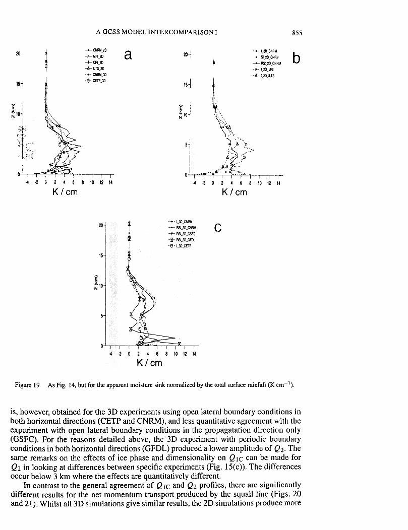
Figure 15. Differences between experiments illustrating the effects of ice-phase paran1etrizations al1d dimen-sionality. (a) The vertical velocity (m s-l), (b) the apparent heat source normalized by the total surfact: rainfall(K cm-l), and (c) the apparent moisture sink normalized by the total surface rainfall (K cm-I). The solid linesshow the differences between experiments with and without an ice-phase parametrization, and the dashed linesshow the differences between the 3D and 2D experiments (see Tables 1 and 4 for an explaJ1ation of the acl;onyms).
850 J .-L. REDELSPERGER el oJ.
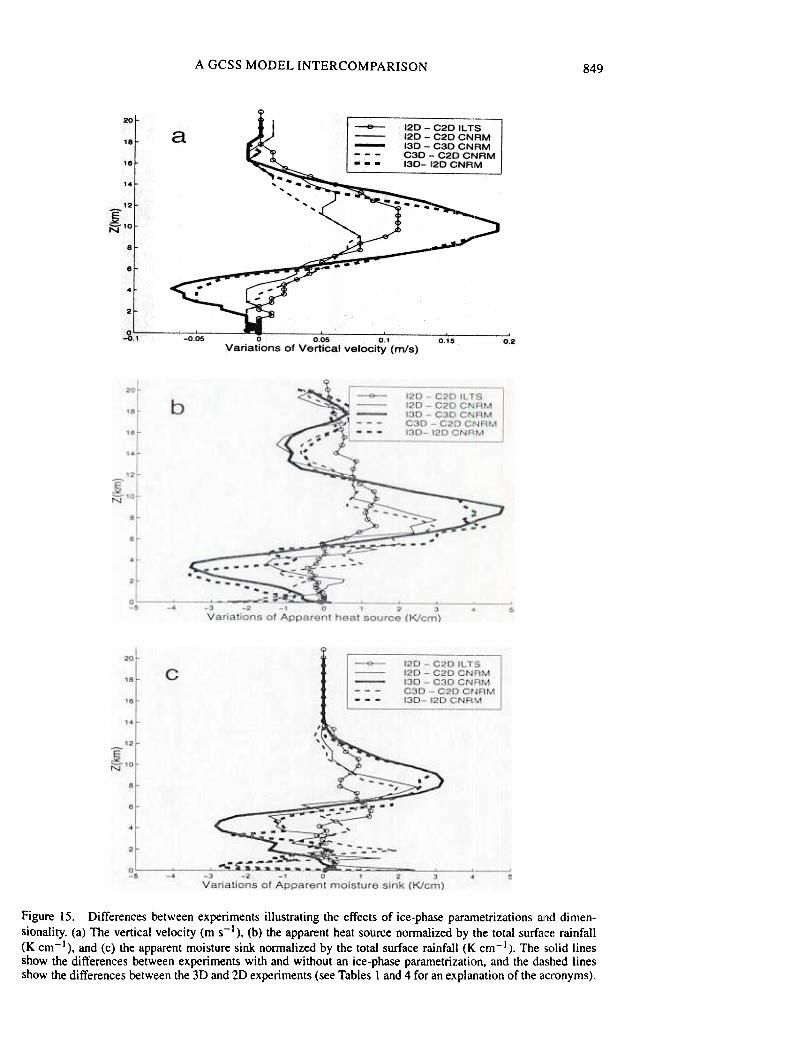
that the inclusion of the third dimension has an eff(~(:t similar in shape and amplitude tothat of including the ice phase (solid lines in Fig. 15(a)). The main effect is clearly toincrease the vertical motion (up to 0.08 and 0.2 m s:-1 for no-ice and ice experiments,respectively) between the heights of 5 and 16 km. A more surprising result is thedecrease observed below 5 km in the 3D run that ificludes an ice phase compared withthe results from the 2D run with ice and the 3D run without ice. This shows that boththe ice-phase parametrization and three-dimensionality are important. Also, the effectsare not simply addititive as no such eff(~ct is obse]:"',red when the ice phase is added inthe 2D runs for both the ILTS and the CNRM modlels, and when the third dimensionis added for the CNRM model without an ice phase. Looking at the same profiles, butin the convective and stratiform regions (not shown:I, reveals that the differences comemainly from the stratiform region where the motions are more intense in the 3D modelsthan in the 2D models. The larger development of tile stratiform region in experimentsincluding the ice phase explain the increase of both upward and downward motionspresent in the stratiform region.
Typical vertical profiles of the rain water content are shown in Fig. 16. The maximaare found at altitudes between about 3 and 4 km in models both with and without an icephase, and have similar values in each case. This sug,gests that much of the precipitationis generated by 'warm-rain' processes between the cloud base and the melting level,which is at around 5 km. The 3D exp4~riments with an ice phase tend to show therain maximum at a higher altitudes than comparable 2D experiments. This suggeststhe organization of precipitation differs in the 3D models. The vertical velocity fields(Fig. 10) show indeed that the second core of the upldraught is generally more delayedin the 2D than in the 3D runs. In addition, the updraughts are more intense in the 3Druns than in the 2D runs (Fig. 3), resulting in a lrurger production of ice particles inthe 3D runs. Rain produced from iced hydrometeor melting is then larger in the 3Dthan in the 2D models. This also contributes tow'ards producing the rain maximumat a higher altitude. In all experiments, below the l(~vel of maximum rain the verticaltransport and evaporation contribute to give a negati1ve gradient approximately equal to0.02 kg kg-1m-I.
The cloud vertical structure and cloud-top altitud(~ for ice and no-ice experiments arecontrasted by comparing the profiles of total water c:ontent (liquid + solid). As shown inFig. 17, all the no-ice simulations have tiheir maximum total hydro meteor content wellbelow the melting level, whereas the ice..phase mo(jels have the maximum at or abovethe melting level. Cloud tops are lower in the experinrlents without an ice phase (around12 km) than in experiments with an ice phase (around 16 km). Most of the profiles oftotal water content from experiments with ice (Figs. 17(b) and (c)) give qualitativelysimilar profiles, with an increase from 0 at z = 5 km up to a mean value of 0.4 g kg-Iand then a decrease above, as with the iprofile of rain water content (Figs. 16(b) and(c). There are, however, larger variations, in the maxiimum values of total water contentthan in the rain water content. In partic1Jlar, the MI.~I and JCMM 2D models predictmaximum values between 0.55 and 0.7 g kg-I although, as noted above, the JCMMmodel is strongly sensitive in this aspect Ito the ice-particle mean fall-speed.
Looking only at the ice experiments, large differences in ice contents aloft (abovethe melting level) are likely to have a significant imp:act in long-duration simulations inwhich radiative feedbacks playa major role in the evolution of the cloud system (e.g.Krueger 1998). These differences need tlJ be investijgated further. Comparison of totalwater contents for the 2D CNRM and ILrS experim(~nts with and without an ice-phaseparametrization indicates slight changes in the first ~) km, and much greater values for
A GCSS MODEL INTERCOMPARISON 851
---CNAM_2D -MAI_2D-*- OAI_2D -6- IL TS_2D
CNAM_3D -e -CETP _3D
20
a
15
5
-"E,:. 1 0
\ ~::~~=-=::;~N ""'... ;~:~:: x~: ~
~.-'.:;:-- ---
~
>0
0.0 0.05 0.1 0.15 0.2 0.25 0.3 0.35
Rainwater mixing ratio (g/kg)
1_2D_CNRM .SI_2D_CNRM--RSI_2D_CNRM -"* -1_2D_MRI
-~ -1_2D_.JCMM -.~- RI_2D_.JCMM~ RSI_2D_.JCMM -& -1_2D_IL TS
0.4
20
t>15
E~;:::; 10
5
~
x-
0
0.0 0.05 0.1 0.15 0.2 0.25 0.3 0.35Rainwater mixing ratio (g/kg)
1_30_CNRM --RSI_30_CNRM-¥- RSI_30_GSFC ~ RSI_30_GFOL-E!)- 1_30_CETP
0.4
20
c:
15
E;;::;-10
5
0
,5 ,~"~~,,J!;o;; , , " ~_4 -~"A~-
.-0.0 0.05 0.1 0.15 0.2 0.25 0.3 0.35 0.4
Rainwater mixing ratio (g/kg)
As in Fig. 14, but for the rain water content (g kg-l ).Figure 16.
J.-L. REDELSPERGER er al.852
--CNRM_2D -~ MRI_2D-*- ORI_2D --b- IL TS_2D
CNRM_3D -~ -CETP _3D20
15
E~N 10
'..,.~
5
..I I I I
0.1 0.2 0.3 0.4 0.5 0.6 0.7 0.8
Water mixing ratio of tota'! hydrometeors (g/kg)1_2D_CNRM ..SI_2D_CNRM
--RSI_~!D_CNRM -"* -1_2D_MRI
-~ -1_2D_.JCMM --<!>-- RI_2D_JCMM~ RSI_~!D_JCMM -6 -1_2D_IL TS
0
0.0
20
15
~N10
~-~)e>
'--t:;::-, --,~
-',- ;:$- ~ ---
.-:;~5~--~-- -<!;S5
x
~ I I I I
0.1 0.2 0.3 0.4 0.5 0.6 0.7 0.8
Water mixing ratio of tots,l hydrometeors (glkg)
1_3D_CNAM ---ASI_3D_CNAM-¥- ASI_3D_GSFC -H-- ASI_3D_GFDL-E!>- 1_3D_CETP
0
0.0
20
c
15
'-~~N10
"@
5
.........,(!J"
\ .-
I -1 I I
0.0 0.1 0.2 0.3 0.4 0.5 0.6 0.7 0.8
Water mixing ratio of to'tal hydromete,:>rs (g/kg)
0
As in Fig. 14, but for the total water content (liquid + solid) (g kg-I ).Figure 17.
A GCSS MODEL INTERCOMPARISON I 853
the ice runs aloft. The latter effect can be related to the increase of vertical veloc:ity asshown above.
Figures 16(c) and 17(c) both show that the 3D GFDL simulation with periodic lateralboundary conditions along both horizontal directions produces lower mixing ratios forrain and total hydrometeors than the 3D simulations with open boundary conditions.As discussed previously, this behavior is consistent with the absence of a feedback be-tween the scale of the convective system and larger scales. This absence results from theperiodic lateral boundary conditions, which preclude the development of destabilizingdomain-averaged vertical motions (Fig. 14). Differences in model microphysical for-mulations could also explain some of the differences. However, the model with p,eriodiclateral boundary conditions has also been used to simulate a compo~;ite easterly wavein the tropical east Atlantic (Donner et al. 1999). In this latter simulation, the e~ffectsof vertical motions at scales larger than the convective system were imposed throughtendencies in the domain-averaged temperature and humidity fields. Precipitation waswithin 30% of observed values. Therefore, it is very likely that most of the differences inthe precipitation and hydrometeors in Figs. 4(c), 5(c), 6(c), 16(c), and 17(c) arise fromthe imposition of periodic lateral boundary conditions along both horizontal dire,~tionson a relatively small domain.
(d) Impacts on the large scale
One of the main underlying uses of sophisticated CRMs is to be able to diagnose theeffects of mesoscale convective systems on the atmosphere. Furthernilore, the datasetsgenerated by CRMs can be used to evaluate in detail the different aspects of cloudparametrizations used in GCMs (see Bechtold et al. 1999). Using Eq:s. (5) and (:6), theapparent heat and moisture sources (Q I C and Q2 respectively) due to convection havebeen computed from the CRM output for different parts of the system. In the presentpaper, only the total sources normalized by the total surface rainfall are presented. Theunits are expressed in (K day-I)(cm day-I)-1 (or, equivalently, in K cm-I).
Previous studies (e.g. Lafore et al. 1988; Tao et al. 1993) have 5:hown that !;qualllines produce two main effects, namely a strong heating in the free troposphert~ plusa cooling in the boundary layer. As shown in Fig. 18, all experiments exhibit thisoverall behaviour of the apparent heat source. All models predict a cooling at lowlevels which is of order 1-2 K cm-1 (normalized by the rainfall:~ caused by rainevaporation, as previously discussed. However, the vertical profile of heating showsvariations from experiment to experiment and from model to model. The inclusion ofan ice parametrization is important in determining the profiles of QIIC. By releasingadditional latent heat of fusion and generating stronger updraughts, the main effect isto create a second maximum of QIC at a higher altitude. As with previous profiles,differences in the profile of QIC for similar experiments can be relatec! to differences inice-phase parametrization used in each model.
More insight into the effect of ice schemes can be obtained by looking at thedifferences for the same model (ILTS and CNRM) with and without an lice-phase scheme(Fig. l5(b». The ice phase decreases QIC below 5 km and increases it betw(~en 5and 12 km. The amplitude of the variations is different between models, and largerin 3D than in 2D. Comparisons between the 2D and 3D experiment~) (Fig. 15(b» forthe CNRM model show that taking into account the third dimension has an ~~ffectsimilar in shape and amplitude to that of including an ice-phase p2lfametrization, atleast between 5 and 12 km. The main effect is to increase the app,lfent heat slource(up to 3 and 4.5 K cm-1 for the no-ice and ice experiments) between 5 and ]l~~ km.~
854 J.-L. REDELSPERGER et al.
CNRII_20-*- 1IFa_20~ ---0AI_20 : -6- 1.15_20
:' -+- CNRII_~
-~- CETP_~
I
I
, I
0
K/cm
a201 b201
i
15l151
E I
~1'15-
-IE~-1N
5~
I I I
4 6 8 8
K/cm
""I.D_CNFII---~.D.OAI
+ ~_D.GSfC+~_D_Gf!I.'&'I.D.CE1P
c15- ~
,I
r
5-
"'A~t'l\
j0-1 -
.2 0 2 4 8 B
K/cm
E~v 10-'II
Figure 18. As Fig. 14. but for the apparent heat source normalized by the total surface rainfall (K cm
As with the vertical velocity profile, a decrease is observed below 5 km in the 3D runwith an ice phase in comparison with both the 2D run with ice and the 3D run withno ice. The inclusion of both the ice-ph:lse parametrization and three-dimensionality isimportant for detem1ining the profile of QIC. These differences originate mainly fromchanges in the stratiform region since the: convective region is dominated by liquid-phaseprecipitation production below the freezing level. These features can be directly relatedto the differences in the profi)es of verti(:al velocity as discussed above (Fig. 15(a)).
Similar results to Q I C are obtained v/hen comparing the vertical profiles of apparentmoisture sinks, Q2, normalized by the to,tal surface rainfall (Fig. 19). All models predicta drying of the atmosphere. One difference is at near-surface levels where some modelspredict no moistening whereas some 2D models predict moistening in the boundarylayer. Overall, the differences are larger for Q2 than for Q\c. A rather good agreement
, -+- 1_2D_CNRM
...".. .51 20 CNRM, --x., --RSI_2D_CNRM
.-'* -I 20 MAl:, .~- 1:20:/lT5
I
I --""'"
0 I
0.2 0 2 4 6
A GCSS MODEL INTERCOMPARISON I 855
-+- CNRM_2D
-j(- MRI_2D
-+- ORI_2D-A- ILTS_2D-+- CNRM_3D
-(9- CETP_3D
-+- 1_2D_CNAM
.SI_2D_CNAM-+- RSI_2D_CNAM
-*- 1_2D_MAI
-6- 1_2D_ILTS
;
a20- b2O-JI
*
15~151
K/cm
E I~10~N I
'~' , , " ,
" ,", ,
'~:~,::'-\I ".
5-i 'x! "'...'.-, ..'1 ::xI .'!!0 ' roc, i I I !
-4 .2 0 2 4 6 8 10 12 14
K/cm
5-
(~
As Fig. 14, but for the apparent moisture sink normalized by the total surface rainfall (K cm-l).Figure 19.
is, however, obtained for the 3D experiments using open lateral bounldary conditions inboth horizontal directions (CETP and CNRM), and less quantitative agreement with theexperiment with open lateral boundary conditions in the propagata1:ion direction only(GSFC). For the reasons detailed above, the 3D experiment with periodic boiundaryconditions in both horizontal directions (GFDL) produced a lower amplitude of (;~2' Thesame remarks on the effects of ice phase and dimensionality on Ql': can be made forQ2 in looking at differences between specific experiments (Fig. 15(c». The diffe:rencesOccur below 3 km where the effects are quantitatively different.
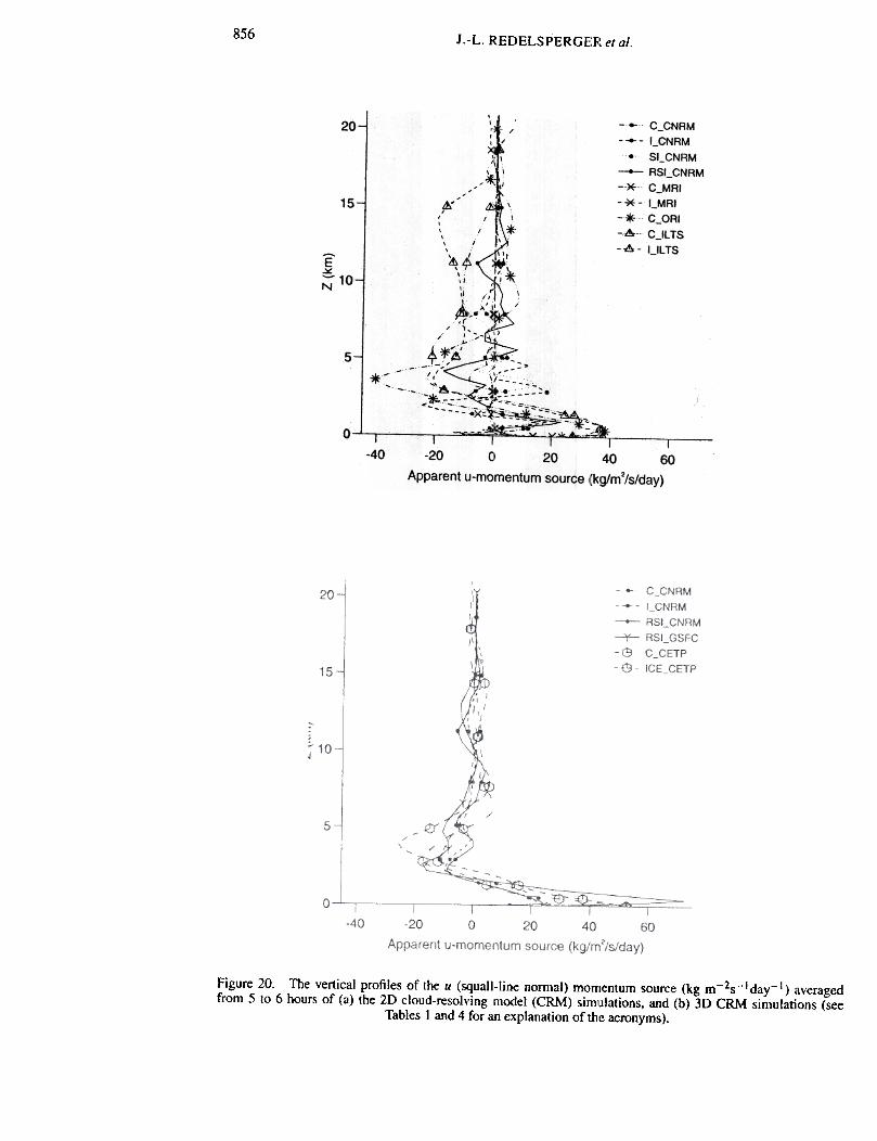
In contrast to the general agreement of Q lC and Q2 profiles, there are significantlydifferent results for the net momentum transport produced by the squall line (Figs. 20and 21). Whilst all 3D simulations give similar results, the 2D simulations produce more
! IN
0
856 J.-L. REDELSPERGE~Fl et a/.
Figure 20. The vertical profiles of the u (squall-lin'~ noffilal) momentum source (kg m-2s-1 day-I) averagedfrom 5 to 6 hours of (a) the 20 cloud-resolving moc!el (CRM) simllllations, and (b) 3D CRM simulations (see
Tables I and 4 for an e~;planation of the acronyms).

A GCSS MODEL INTERCOMPARISON I 857
-+- C_CNRM
-+- I_CNRM
--RSI_CNRM+ RSI_GSFC-(9- C_CETP-(9- I_CETP
20
I.:I j,
15
E~~ 10
5
0
I
I
:~I\IJ I '. I
i'.
---
.15 .10 .5 0 5 10 15 20 25
Apparent v-momentum source (kgim2/s/day)
Figure 21. The vertical profiles of v (squall-line parallel) momentum source (kg m-2s-1 day-I) averaged from5 to 6 hours of the 3D cloud-resolving model (CRM) simulations (see Tables I and 4 for an explanation of the
acronyms).
oscillatory behaviour, though the low levels are more coherent. This result is consistentwith the previous discussion about the differences between the momentum profiles,and it supports a recommendation for using a 3D framework or, if not possible (e.g.for computational considerations), a 2D framework with a relaxation towards a meanhorizontal wind (initial or observed). This latter approach has been used with successfor the second case (see introduction) selected by the Precipitating Convective CloudSystems Group of the GCSS (Krueger 1998). Although the use of a 2D model precludesthe study of momentum transport, it keeps the wind profile closer to the observations, akey parameter in determining the convective organization. Examinaltion of the profilesof momentum sources from the 3D simulations suggests that, on avt~rage, the effect ofthe convective system is to decrease the shear.
CONCLUSION5
This GCSS intercomparison study has, for the first time, enabled the comparison ofeight CRMs for the case of an oceanic tropical squall line observed during the TOGA-COARE experiment. Numerous papers have shown that the overall squall-line structureis determined from the cold pool and environmental wind shear (e.g. ~rhorpe et al. 1982;Redelsperger and Lafore 1988; Rotunno et al. 1988). This explains why, over~lli. boththe 2D and 3D models performed well in simulating most of the main. observed featuresof the squall line, in particular its structure and propagation. The g,oal of the present

858 J.-L. REDELSPERGER et a.l.
work was also to perforn1 a first quantitcltive interco,mparison of quantities describingthe convective intensity and the key features for pclrametrization in GCMs. Most ofthe models were also able to predict a similar rainlfall and integrated water contentevolutions and agreed quantitatively. The apparent h,eat and moisture sources also had asimilar shape from model to model under some experimental configurations, though toa lesser extent. The 3D experiments with an ice-pha.se parametrization and with openlateral boundary conditions along the direction of :~ystem propagation showed goodagreement for most parameters. Compariison of the 3D simulated fields with the onesderived from two different analyses of airborne Doppler radar data indicated that 3Dmodels with open lateral boundary conditions along the direction of system propagationare able to simulate the proper dynamical structure.
Surface fluxes and radiative processes were foUl1ld to have only a small impact onthe experiments, slightly increasing the intensity of the convection and those quantitiesrelated to the rainfall. This conclusion is based on radiative processes invoked for a shortperiod of time (7 hours). Also, with regarcj to surfacc~ fluxes, squall lines extract most oftheir energy from the ambient atmospheve thanks to their fast propagation. In contrast,some of the results were found to be sensitive to the microphysical scheme and to theframework dimensionality (2D versus 3D).
The line-averaged vertical motion taken from Doppler radar observations duringthe linear stage of the squall line displayed a double-peaked updraught structure. Thisfeature was also simulated by the 3D CRMs. Thc~ second peak at around 10 kmin height was obtained only when an i,ce-phase parametrization was used. The 2Dsimulations with an ice-phase parametrization also exhibited this structure, although.t and z locations of these peaks differed. Snapshots indicate that the 2D experimentsexhibited large temporal variability in their structun~s; this feature was also observedin the time series. The 20 simulations produced smaller values of maxima and minimaof vertical velocity than the 3D ones (about half the magnitudes). For both 2D and3D experiments the downdraught values were about half the updraught ones, a resultalso true for the mean values in the convective region. The use of periodic lateralboundary conditions along the direction of system! propagation over a small domainwas found to decrease the intensity of the system, ~~iving a smaller stratiform region,lower vertical velocities and smaller water contents. In this case, full advection ofhydrometeors ejected from the convective region was not allowed. Confirn1ing thispoint, the 2D experiments using a larg'~ domain (1000 km) together with periodiclateral boundary conditions were well able to produce stratiforn1 regions and showeda reasonable quantitative agreement for global parameters (such as the integrated watercontent and rainfall) with the 3D model n~sults.
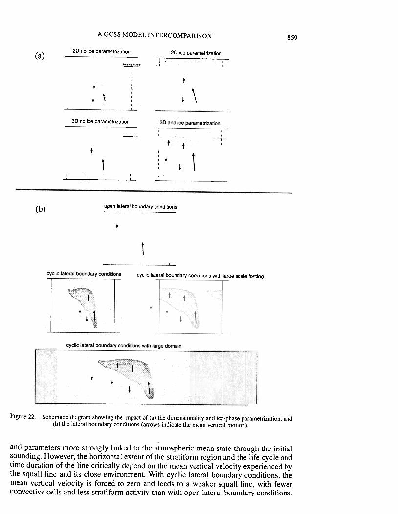
The impacts of the dimensionality, i,ce phase and lateral boundary conditions aresummarized in Fig. 22. Ice-phase processes tend to increase both the vertical and thehorizontal extent of the convective systl~m significantly (Fig. 22(a)). The horizontalextent of the stratiform part depends, however, on the ice-phase parametrization; thisis especially true in 2D. The squall line ,exhibits much less temporal variability in 3Dthan in 2D, with a less pronounced tilting. The 3D framework leads to the developmentof deeper convective cells and a larger stratiform re!~ion (Fig. 22(a)). In this respect, theice-phase parametrization and the third dimension ,l(:t in much the same way, althoughthrough different (by nature) processes. The model sensitivity to the lateral boundaryconditions (Fig. 22(b)) is directly relate~d to the impact of the interactions betweenthe convective system and its large-sca.le environment. Different choices of lateralboundary conditions do not modify the basic convec:tive features, such as the intensityof convective up- and downdraughts, thl~ maximum vertical extent of the squall line,
A GCSS MODEL INTERCOMPARISON 859
20 no ice parametrization 20 ice parametrization(a) .'
I '..
..I
t
\~
3D no ice parametrization
I
,'
t I
I
I ,II
I
I
~, ,.I
open lateral boundary conditions(b)
t
cyclic lateral boundary conditions with largt~ scale forcing
Figure 22. Schematic diagram showing the impact of (a) the dimensionality and ice-phase parametrization, and(b) the lateral boundary conditions (arrows indicate the mean vertical motion).
and parameters more strongly linked to the atmospheric mean state through d\e~ initialsounding. However, the horizontal extent of the stratiform region aruj the life c:ycle andtime duration of the line critically depend on the mean vertical velocity experienlced bythe squall line and its close environment. With cyclic lateral boundary conditic,ns, themean vertical velocity is forced to zero and leads to a weaker squ2111 line. with fewerconvective cells and less stratiform activity than with open lateral boundary conditions.
860 J.-L. REDEIJSPERGERetal.
Using a much larger domain than the width of the squall line itself (Fig. 22(b)) can toovercome this deficiency. When a mean large-scale ascent is applied to a domain withcyclic lateral boundary conditions (as in the second case of GCSS) the intensity of theconvective system increases, although spurious effect~~ can arise owing to the horizontaladvection of hydrometeors.
Examination of the wind profile evolution and momentum sources from the 3Dsimulations suggests that, on average, the squall line has the main effect of decreasingthe shear. This result is in contrast to th(~ behaviour of African squall lines observedand simulated during the COPT81 expeilment, whe~re an increase in shear was foundin some parts of the atmosphere. One possible reas,on, in agreement with the recentdetailed analysis of Trier et at. (1998), is the relatively small linear portion of thepresent system, with different types of flow in the northern, southern and central partsof the squall line. The COPT8l case looked more like the central part of the presentsystem. The 2D experiments were not abll~ to capture the same evolution in wind. Theypredicted an increase of the jet and gene~rally led to large vertical oscillations of theline-normal component of the wind. The,oretical explanations based on the continuityequation have been given. The treatment of lateral boundary conditions is also importantfor this matter. Thus, periodic lateral boundary conditions preclude any change in thevertical average of u-momentum in each column of the 2D models. This result suggeststhat in 2D it is better to relax the domain-average horizontal wind towards observedwinds. This approach has been successfully followed for the other intercomparisoncase (Krueger 1998) and, whilst this precludes the study of momentum transport, thewind profile stays close to the observations, which is a key factor in determining theconvective organization.
It is worth noting that this difficult and long exercise was found to be very useful bythe participants in allowing them to checl[( many parts of their codes and to find someerrors. Clearly more confidence in the codes has be~c~n gained from this exercise. It isclear that this first intercomparison has tOI be considered only as a first step. Neverthe-less, similarities and differences between 2D and 3D models have been identified onthe basis of numerous experiments with the eight different models. Also, the resultsare a motivation to work to reduce the uncertaintie~. coming from the microphysicalparametrizations. As an example, discrepancies found with one of the 2D models whencomparing with other models were reduc(~d when the mean fall speed of cloud ice wasincreased. Though ice processes are generally thought to be important for time-scales;:: I day, the present results show that the~y also nee:dl to be considered for time scalesof few hours. This emphasises the impol1ance of further study into the sensitivity ofmodels to microphysical parametrizations for such case studies. In order to improve ice-phase parametrizations, the authors recornmend the design of a field experiment fullydedicated to this fundamental issue. This should also include within the dataset in-situobservations of the upper-tropospheric cloud microphysical properties, measurementsof which were unavailable during TOGA--COARE.
Finally, diagnostics issued from the intercompalison illustrate that datasets fromCRMs validated against observations can be used to evaluate and develop cloud param-etrizations used in large-scale models. Such an approach is presented in a companionpaper (Bechtold et at. 1999).
ACKNOWLEDGEMENTS
We would like to express our gratitude to Dr M. J\1oncrieff who led the GCSS Pre-cipitating Convective Clouds Working Group during the project. Enthusiastic support
A GCSS MODEL INTERCOMPARISON I 861
from Prof K. Browning, the chainnan of European Cloud-REsolving Modelling project(EUCREM) and GCSS, is gratefully acknowledged. Support from Prof S. Kruegerwas also appreciated. Discussions at the initial stage of the project with Drs S. Trier,M. A. LeMone and D. Jorgensen were helpful in setting up the initial conditions. Re-search at the CNRM/GAME and the Joint Centre for Mesoscale Metl~orology (JCMM)were partly funded by the European Commission through the EUCRJSM project .ENV 4CT95 0107. One of the authors of this paper (K. Nakamura) would like to thank theCenter for Analysis and Prediction of Stonns (University of Oklahoma), which wasresponsible for the development of the Advanced Regional Prediction System model.Runs perfonned at the Centre d'etude des Environnements Terrestre e:t Planetaires havebenefitted from help ofT. Biju, J. P. Lafore, J. P. Pinty, P. Jabouille and J. Stein. Two ofthe authors (W. K. Tao and S. Lang) were supported by the National Aeronautics andSpace Administration (NASA) Tropical Rainfall Measuring Mission, and their comput-ing resources were provided by the NASA Goddard Space Flight Center. The JCMM issupported by the UK Meteorological Office and the University of Reading.
2000
REFERENCES
A GCSS model intercomparison for a tropical squall lineobserved during TOGA-COARE. Ui: Intercomparison ofsingle-column models and a cloud-resolving model.. Q. J. R.Meteorol. Soc., 126,865-888
An intercomparison of radiatively driven entrainment and turbu-lence in a smoke cloud, as simulated by different numericalmodels. Q. J. R. Meteorol. Soc., 125, ~;91-424
1999
Bechtold. P.. Redelsperger. J.-L..Beau. I.. Blackburn. M..Brinkop. S.. Grandpeix. J.- Y.Grant. A.. Gregory. D..Guichard. F.. Hoff. C. andloannidou. E.
Bretherton. C. S.. MacVean. M. K.Bechtold. P.. ChIond. A..Cotton. W. R.. Cuxart. J..Cuijpers. H..Khairoutdinov. M..Kosovic. B.. Lewellen. D..Moeng. C.-H.. Siebesma. P..Stevens. B.. Stevens. D. E..Sykes. I. and Wyatt. M. C.
Caniaux. G.. Redelsperger. I.-L.and Lafore. J.-P.
1994
Caniaux. G.. Lafore, J.-P. andRedelsperger,J.-L.
1995
1988Chen, S. and Cotton, W. R.
Chong, M., Amayenc, P.,Scialom, G. and Testud, J.
1987
1999Donner, L. J., Seman, C.J. andHemler, R.S.
Fovell R. G. and Ogura, Y. 1988
1992Gates, W. L.
1993Held I. M., Hemler. R. S. andRamaswamy. V.
Houze. R. A. 1977
199\Ikawa, M. and Saito, K.
A numerical study of the stratifoml region of a fast-moving squallline. Part I. General description, and water and heat blldgets.J. Almas. Sci., 51, 2046--2074
A numerical study of the stratifoml region of a fast-moving squallline. Part n: Relationship between m:lSS, pressure and mo-mentum fields. J. Almas. Sci., 52, 331--352
The sensitivity of a simulated extratropical mesoscale convectivesystem to longwave radiation and ice-phase microphysics.J. Almas. Sci., 45, 3897-3910
A tropical squall line observed during the COJYr81 experiment inWest Africa. Part I: Kinematic structUI'e inferred from! dual-doppler radar data. Man. Wealher Rev.. lIS, 670-694.
Three-dimensional cloud-system modeling of GATE convection.J. Almas. Sci., 56.1885-1912
Numerical simulation of a mjdlatitude squctllline in two dimen-sions. J. Armas. Sci., 45, 3846--3879
AMIP: The atmospheric model intercomparison projec:t. Bull.Ame/: Metearol. Soc., 73, 1962-1970
Radiative-convective equilibrium with explicit two-dimensionalmoist convection. J. Almas. Sci., 50, 3S111-3927
Structure and dynamics of a tropical squall line system observedduring GATE. Man. Weal her Rev., 105" 1540-1567
'Description of a nonhydrostatic model developed at the Fore-cast Resean;h Department of the MFU'. MRI Tech. Rep.28, (available from the Meteorology Research Institute,Tsukuba, Japan)
Structure and evolution of the 22 February 1993 TOGA-COAREsquall line: Observations of precipital:ion. circulation, andsurface energy fluxes. J. Armas. Sci., s.I, 1961-1985
1997Jorgensen. D. P.. LeMone. M. A.and Trier, S. B.

862 J.-L. REr:'ELSPERGER et al.
Krueger. S. K. 1998
Lafore, J.-Po, Redelsperger, J.-L.and Jaubert, G.
1988
'A (XSS intercomparison of cloud-resolving models based onTOGA-COAFE observations'. Pp113-l27 in Proceedingsof the workshop in 'New insights and approaches to convec-tive pararneu;zation', European Centre for Medium-RangeWeather Fort',casts, Reading, UK
Comparison between a three-dimensional simulation and Dopplerradar data of a tropical squall line: Transports of mass, mo-mentum heat and moisture. J. Armos. Sci.. 45, 3483-3500
The Meso-NH atrnospheric simulation system. Part I: Adiabaticformulation and control simulations, Ann. Geophys.. 16,90-109
1998Lafore, J.-P., Stein, J., Asencio, N.,Bougeault, P., Ducrocq, V.,Duron, J., Fisher, C.,Hireil, Ph., Mascart, P.,Pinty, J. P., Redelsperger, J.-L.,Richard, E. andVil-Guerau de Arellano, J.
LeMone, M. A., Jorgensen, D. P.and Smull, B. F.
1994
LeMone, M. A., Zipser, E. J. andTrier, S. B.
1998
1983
1997
'The impact of two convective systems of sea-surface stressesin COARE'. Pp. 40-44 in Preprints of the 6th conferenceon mesoscale processes. American Meteorological Society,Portland. USA
The role of environmental shear and CAPE in determining thestructure and evolution of mesoscale convective systems dur-ing TOGA-COARE. J. Atmos. Sci., 55,3493-3564
Bulk parameterization of the snow field in a cloud model. J. Cli-mate Appl. Meteorol., 22, 1065-1092
Dynamical influence of microphysiscs in tropical squall lines:A numerical study. Mon. Weather Rev.. 125, 2193-2210
Simu'!ation of a S1.ratocumulus-topped PBL: Intercomparisonamong different numerical codes. Bull. Arne!: Meteorol. Soc..77,261-278
1996
GEWEX Cloud System Study (GCSS) Working Group 4: Precip-itating convective cloud systems. Bull. Arner. Meteorof. Soc.,'78,831-845
1997
Lin, Y. L., Farley, R. D. andOrville, H. D.
Liu, C., Moncrieff, M. W. andZipser, E. J.
Moeng, C.-H., Cotton, W. R.,Bretherton, C. S., Chlond, A.,Khairoutdinov, M.,Krueger, S. K.,Lewellen, W. S,MacVean, M. K.,Pasquier, J. R., Rand, H. A,Siebesma, A. P., Sykes, R. I.and Stevens, B.
Moncrieff M. W., Gregory, D.,Krueger, S. K.,Redelsperger, J.-L. andTao, W. K.
Montmerle, Th. and Lemaitre, Y. 1998
Nicholls. M. E. 1987
Pinty. J. P. and Jabouille. P. 1998
1986Redelsperger, J.-L. andSommeria, G.
Redelsperger, J.-L. and Lafore, J.-P. 1988
1996Redelsperger J.-L., Gregory. D.,Krueger. S. K.,Moncrieff, M. W. andTao, W. K.
Thre(:-dimensional variational data analysis to retrieve thermo-dynamical fields from various nested wind measurements..f. Armos, Ocean. Techno/" 7, 64G--665
A comparison of the results of a two-dimensional numerical sim-ulation of a tropical squall line with observations, Mon.'Weather Rev., 115,3055-3077
'A mixed-phased cloud parameterization for use in a meso-~;cale non-hydrostatic model: simulations of a squall line;md of orographic precipitation', In the Proceedings of the<:Ioud physics conference, American Meteorological Society,Boston, USA
Three~dimensional simulation of a convective storm: sensitivity5:tudies on subgrid parameterization and spatial resolution..I'. Armos. Sci" 43, 2619-2635.
Three-dimensional simulation of a tropical squall-line: Convec-tive organization and thermodynamic vertical transports,J'. Armos. Sci., 45,1334-1356
'GE~fEX Cloud System Study (GCSS) on precipitating convec-tive cloud sytems model intercomparisons. CASE I: Tropical(ICeanic convection of TOGA-COARE'. Unpublished (avail-able from J. -L. Redelsperger, CNRM/GAME, 42 AvenueCoriolis, 31057 Toulouse, France, or fromhttp://www.cnrm.meteo.fr/gcss/)
Convt:ction in TOGA-COARE: Horizontal scale, morphology,and rainfall production, J. Armos. Sci., 55,2715-2729
A theory for strong, long-lived squall lines. J. Armos. Sci., 45,1.f63-485
1998Rickenbach, T. M. andRutledge, S. A.
Rotunno, R., Klemp, J. B. andWeisman, M. L.
1988

A GCSS MODEL INTERCOMPARISON 863
1988Rutledge, S.A., Houze, R. A. Jr.,Biggerstaff, M. I. andMatejka, T.
Saito, K. and Kato, T. 1996
1997
The Oklahoma-Kansas mesoscale convective system of 10--11June 1985: Precipitation structure and single-Doppler radaranalysis. Mon. Weather Rei'., 116,1409-1430
On the modification of the MRI nonhydrostatic nesting model.Tenki, 43, 369-382
Shipboard radar rainfall patterns within the TOGA COARE IFA.Bull. Arne!: Meteorol. Soc., 78,2817-2836
Short, A. D., Kucera, P. A.,Ferrier, B. S., Gerlach, J. C.,Rutledge, S. A. andThiele, O. W.
Shutts, G.J. and Gray, M. 1994
1996
A numerical modelling study of the geostrophic adjustment pro-cess following deep convection. Q. ,f. .R. Meteoro{. Soc., 120,1145-1178
Intraseasonal oscillations in 15 atmospheric general circulationmodels: results from an AMIP dial~nostic subprojl~ct. Clim.Dynamics, 12, 325-357
Sl.ingo J. M.. Sperber. K. R..Boyle. J. S., Ceron, J. P..Dix, M., Dugas, B.,Ebisuzaki, W.. Fyfe, J.,Gregory, D., Gueremy. J. F.Hack, J., Harzallah, A.,Inness, P.. Kitoh. A.,Lau, W. K., McAvaney, B.,Madden. R. Mathews, A..Palmer, T. N., Park, C.-K.,Randall, D. and Renno, N.
Swann, H. A. 1996
Tao, W.-K. and Simpson, J. 1989
Tao, W.-K., Simpson, J., Sui. C.-H.,Ferrier, B., Lang, S. Scala. J.,Chou. M.-D. and Pickering, K.
Tao, W.-K.. Simpson. J. andFerrier. B.
1993
1997
Thorpe, A. J.. Miller M. J. andMoncrieff. M. W.
1982
1996Trier, S. B., Skamarock, W. C.,LeMone, M. A, Parsons, D. B.and Jorgensen, D. P.
Trier, S. B., Skamarock, W. C. andLeMone, M. A
1997
Trier, S. B., LeMone, M. A andSkamarock, w. C.
1998
1996
'The development and validation of ,a microphysics; schemefor cloud-resolving model studies of deep convection'.Ph.D. thesis, University of Reading, UK
Modeling study of a tropical squall type c:onvective lint:. J. Atmas.Sci., 46, 177-202
The Goddard cumulus ensemble model. Part I: Model description.Terr: Atmas. Ocean. Sci., 4, 35-72
Heating, moisture, and water budgets of tropical and midlatitudesquall lines: Comparisons and sensitivity of longw'ave radi-ation. J. Atmas. Sci.. SO, 673-690
'Simulations of mesoscale convective systems'. pp. 77--112 in theProceedings of the ECMWF workshop on new insights andapproaches to convective parametrization, Europl~~m Centrefor Medium-Range Weather Forecasts, Shinfield F'ark, Read-ing,UK
Two-dimensional convection in non-constant shear: A model ofmid-latitude squall lines. Q. J. R. M'eteara/. Sac., 108,739-762
Structure and evolution of the 22 FebruaIY 1993 TOGf\--COAREsquall line: Numerical simulations. .r. Atmas. Sci., 53, 2861-2886
Structure and evolution of the 22 FebruaIY 1993 TOGA--COAREsquall line: Organization mechanisms inferred from! numeri-cal simulation. J. Armas. Sci., 54, 386-407
Effect of three-dimensional structure on the stormwide horizontalaccelerations and momentum budgl~t of a simulatl~d squallline. Man. Weather Rev., 126,2580-2598
The impact of a surface layer on TOGA-COARE cloud systemdevelopment. Man. WeatherRe,,:,l~~, 2753-2763
'ARPS Version 4.0 User's Guide'. Unpublished (available fromthe Center for Analysis and Prediction of Storms, Universityof Oklahoma, 100 E. Boyd St., Nonnan OK 73019, USA)
Numerical simulations of tropical squall line clusters: Two-dimensional model. J. Metearo/. Soc. Japan. 64,469-491
Mesoscale and convective scale downdrafts as distinct compo-nents of squall-line circulation. Mon. Weather Rev., 105,1568-1589
Wang, Yo, Tao, Wo-K. andSimpson, J.
Xue, Mo, Droegemeier, K. K.,Wong, Yo, Shapiro, Ao andBrewster, K.
Yoshizaki, M.
1995
1986
Zipser, E. J. 1977