Embed Size (px)
Citation preview
A functional coefficient model view of the
Feldstein-Horioka puzzle
Helmut Herwartz∗ and Fang Xu†
November 2006
Abstract: What does the saving-investment (SI) relation really measure and how
should the SI relation be measured? These are two of the most discussed issues trig-
gered by the so called Feldstein-Horioka puzzle. Based on panel data we introduce a
new variant of functional coefficient models that allow to separate long and short to
medium run parameter dependence. We apply the latter to uncover the determinants
of the SI relation. Macroeconomic state variables such as openness, the age depen-
dency ratio, government current and consumption expenditures are found to affect
the SI relation significantly in the long run.
Keywords: Saving-investment relation, Feldstein-Horioka puzzle, functional coeffi-
cient models,
JEL Classification: C33, E21, E22
∗Institute for Statistics and Econometrics, Christian-Albrechts-University of Kiel, Olshausenstr.40-60, D–24118 Kiel, Germany, [email protected].
†Corresponding author. Institute for Statistics and Econometrics, Christian-Albrechts-Universityof Kiel, Olshausenstr. 40-60, D–24118 Kiel, Germany, [email protected], Fax: (+49)431-880-7605.
1

1 Introduction
“How internationally mobile is the world’s supply of capital?” This is the question
investigated by Feldstein and Horioka (1980), henceforth FH (1980). By means of
a between regression for OECD countries, FH (1980) document a strong correlation
linking the domestic investment and saving, which is argued to be at odds with capital
mobility. Following FH (1980) one would expect that under perfect capital mobility
the correlation between a country’s saving and investment ratio should be small. As
such the diagnosed high correlation is in contrast to established theoretical frameworks
in open economy macroeconomics and also to the believe that capital markets have
experienced substantial liberalization.
The so-called “Feldstein Horioka puzzle” (FH puzzle) has provoked a lively dis-
cussion in both theoretic and empirical literature. Two of the most investigated ques-
tions are: What does the saving-investment relation really measure and how should
the saving-investment relation be measured? To answer the first question, various
determinants of the SI relation have been suggested in the theoretical literature such
as population growth (Obstfeld 1986), the intertemporal budget constraint (Coakley,
Kulasi and Smith 1996, Taylor 2002), output fluctuations in non-traded goods (Tesar
1993), or current account targeting (Artis and Bayoumi 1992). Since the intertem-
poral budget constraint seems to be one of the most convincing reasons for a high
SI relation, most recent empirical investigations for the SI relation are concentrating
on a potential cointegration relation between saving and investment.1 Thereby, error
correction models are suggested as the suitable framework to measure the SI rela-
tion.2 However, no unique evidence for a cointegration relation between saving and
investment is found. Compared to the abundant empirical investigations for the in-
tertemporal budget constraint, empirical contributions linking all other determinants
of the SI relation are rather scarce. A few exceptions and identified factors are Sum-
mers (1988) (government budget balance), AmirKhalkhali, Dar and AmirKhalkhali
(2003) (government size), Kasuga (2004) (financial structures) and Sachsida and Cae-
tano (2000) (the variability between external and domestic saving). Furthermore, in
these contributions there exists no unique model to measure the SI relation along with
potential determinants.
In this paper, we suggest a new semiparametric approach to investigate the de-
terminants of the SI relation. The latter is derived as a bivariate generalization of
functional coefficient models (Cai, Fan and Yao 2000). We adopt a new bootstrap
based venue of inference which is suitably immunized against adverse effects of (mild)
under- or oversmoothing of semiparametric functional estimates. To identify poten-
tial determinants of the SI relation the formalized semiparametric model is suitable
1Abbott and Vita (2003), Gulley (1992), Ho (2002a), Ho (2002b), Leachman (1991), Lemmenand Eijffinger (1995), Haan and Siermann (1994), Miller (1988), Vita and Abbott (2002).
2Bajo-Rubio (1998), Coiteux and Olivier (2000), Jansen (1996), Jansen and Schulze (1996),Jansen (1998), Moreno (1997), Ozmen and Parmaksiz (2003b), Ozmen and Parmaksiz (2003a),Pelagidis and Mastroyiannis (2003), Pelgrin and Schich (2004), Schmidt (2001), Sinha and Sinha(2004), Taylor (1996), Taylor (1998).
2

to cope with cross sectional heterogeneity, time and factor dependence. It allows to
separate deterministic from measurable economic conditions characterizing the em-
pirical SI relation over time. Moreover, it allows to distinguish long and short run
factor impacts on the SI relation.
We analyze annual data spanning the period 1971 to 2002 for various (partly
overlapping) cross sections characterizing the world economy, developing countries,
the OECD, the EU and the Euro area. With respect to the choice of potential factor
variables we rely on recent studies by Edwards (1995), Debelle and Faruqee (1996),
Milesi-Ferretti and Razin (1997), Milesi-Ferretti and Razin (1998), Masson, Bayoumi
and Samiei (1998), and Chinn and Prasad (2003). The employed factor variables
allow a classification into three groups: Potential determinants of saving, investment
or the current account balance and factors describing the integration of goods and
financial markets. In addition, the scope of variables measuring the dependence of
the SI relation on country size is addressed.
From functional coefficient models, an economies’ degree of openness, its age de-
pendency ratio and government current and consumption expenditures are identified
to have a significantly negative influence on the SI relation in the long run. Besides,
countries with high GDP (measuring the effect of country size) are more likely to
have a high SI relation. According to these results, the interpretation of a high SI
relation as a signal for low capital mobility in FH (1980) has to be treated with care.
As a consequence, empirically high SI relations could reflect goods market friction,
demographic development or fiscal consolidation rather than being puzzling.
The remainder of the paper is organized as follows: In the next Section we briefly
sketch some core theoretical contributions provoked by FH (1980). In Section 3 we
initiate our empirical analysis by highlighting that the empirical SI relation has ex-
perienced some weakening over more recent time periods and might be driven by
measurable economic factors. Given that the link between domestic saving and in-
vestment is likely heterogeneous over time as well as factor dependent we introduce a
semiparametric approach to evaluate the SI relation in Section 4. We derive the new
framework from univariate functional coefficient models, and discuss briefly model
representation, estimation, implementation and inferential issues. Empirical results
obtained from the latter venue of modeling are provided in Section 5. Section 6 sum-
marizes briefly our main findings and concludes. More detailed information on the
investigated (cross sections of) economies and factors is given in the Appendix.
2 Economic models explaining a high SI relation
In this section, we sketch briefly some of the leading explanations offered in macro-
economics to explain a high SI relation. For a detailed review over the literature
on the FH puzzle the reader may consult Coakley, Kulasi and Smith (1998). From
the viewpoint of economic theory, firstly, general equilibrium models have been con-
structed that allow a high SI relation in response to exogenous shocks under high or
3

perfect capital mobility. By means of a life-cycle model Obstfeld (1986) demonstrates
that, given a rise in the population growth rate, both the saving and the investment
ratio increase. Mendoza (1991) constructs a real-business-cycle model of a small open
economy with moderate adjustment costs and small variability and persistence of
technological shocks. The latter turns out to be consistent with a positive correla-
tion between domestic saving and investment, although financial capital is perfectly
mobile.
Secondly, the stationarity of the current account balance implied by the long run
intertemporal budget constraint (solvency constraint) could induce a high SI relation.
By construction, saving minus investment equals the current account balance. Thus, a
close SI relation might reflect stationarity of the current account. Introducing a market
determined risk premium on borrowing, Coakley, Kulasi and Smith (1996) show that
the long run solvency constraint implies a stationary current account. For the case
of a simple Solovian economy with stochastic growth, Taylor (2002) demonstrates
that stationarity of the current account is a sufficient condition for the long run
intertemporal budget constraint to hold. In this vein of economic models a high SI
association reflects the solvency constraint, but not necessarily capital immobility.
However, the empirical evidence on the stationarity of current account balances is
weak or mixed.
In the third place a high SI relation may be due to a government targeting the
current account balance. Artis and Bayoumi (1992) argue that the current account
balance was an important target for monetary policy in the 1970s, but not in the
1980s. This policy change appears to correspond to a reduction in the SI relation
among OECD countries in the 1980s.
A recent perspective on the latter two issues that takes the bounded nature of
current account measures in unit root tests into account is provided in Herwartz
and Xu (2006c). They argue that the current account balance is a bounded non-
stationary process and empirical rejections of the unit root hypothesis might be due
to the existence of bounds in the sense of policy controls or crises. Thus, the high
SI relation might be partially caused by the existence of the bounds on the current
account imbalances.
Finally, the goods market, not the capital market, may be seen as the binding con-
straint linking domestic saving and investment. From this perspective, Tesar (1993)
demonstrates that a model with stochastic fluctuations in the output of non-traded
goods is consistent with a high SI association. In case non-traded goods account for
a significant share of total output, consumer preferences over traded and non-traded
goods and over the intertemporal allocation of consumption may introduce low cross-
country correlations of aggregate consumption and an optimal portfolio biased towards
claims on domestic output. Describing the so–called consumption correlations puzzle
(Backus, Kehoe and Kydland 1992) and the home-bias portfolio puzzle (French and
Poterba 1991), the latter effects are in line with a high SI relation. Comparably, Obst-
feld and Rogoff (2000) demonstrate that moderate transactions costs of international
trade may cause a substantial difference in real interest rates in spite of full financial
4

market integration. In turn, real interest rate differentials might give rise to a high
SI relation.
3 Preliminary analyses
Having reviewed theoretical approaches to modeling the SI relation, we introduce the
data and motivate the use of alternative cross sections in this section. Furthermore,
stylized features of the empirical SI relation, as e.g. its downward trending behavior,
will be illustrated by means of standard between regressions as in FH (1980) and time
dependent regressions as adopted by Sinn (1992) or Blanchard and Giavazzi (2002).
Finally, the issue of factor dependence is addressed.
3.1 The data
In the empirical literature on the SI relation, most authors concentrate on one or two
specific cross sections such as OECD members, EU countries, the Euro area, large or
less developed economies. In this paper, we investigate a set of specific cross sections,
and a general cross section sampled from all over the world and containing as many
economies as possible conditional on data availability. The latter is one of the largest
cross sections that has been considered to analyse the SI relation. Distinguishing
numerous specific cross sections will be useful to reconsider former analyses relating
the SI relation e.g. to the degree of market integration or the state of development.
The large cross section promises a global view on descriptive features of the correlation
between domestic saving and investment and its underlying determinants.
We investigate the SI relation with seven alternative (partly overlapping) cross
sections using annual data from 1971 to 2002 drawn from the World Development
Indicators CD-Rom 2004 published by the World Bank. These cross sections are
composed as follows:
1) The first and most comprehensive sample covers 97 countries from all over the
world (W97), for which most observations of the saving and investment ratio
from 1971 to 2002 are available. For 6 countries data for 2002 are not available.
These missing values are estimated by means of univariate autoregressive models
of order 1 with intercept. Although data for Sao Tome and Principe and Lesotho
are published, these two countries are not included owing to an outstandingly
high negative saving ratio prevailing over quite a long period. A list of all 97
countries contained in W97 is provided in the Appendix.
2) All OECD countries except Czech Republic, Poland, Slovak Republic and Lux-
embourg comprise the second cross section and is denoted with O26. The first
three countries are not included due to data nonavailability. Luxembourg is
often excluded in empirical analyses of the SI relation owing to presumably
peculiar determinants of its savings.
5

3) The third sample we consider covers 14 major countries of the European Union
(E14), which are the O26 countries without Australia, Canada, Hungary, Ice-
land, Japan, Korea, Mexico, New Zealand, Norway, Switzerland, Turkey and
the US. Contrasting this subgroup with O26 may reflect the EU effect on the
SI relation.
4) As the fourth cross section 11 Euro area economies excluding Luxembourg (E11)
are investigated. E11 differs from E14 by exclusion of Denmark, Sweden and
the UK. In the Euro area, there is no exchange rate risk and financial markets
should be more integrated in comparison with the remainder of the EU.
5) To offer a ’complementary’ view at the link between market integration and the
SI relation, we investigate a fifth cross section defined as O26 minus E11. Here
we focus on weaker forms of market integration and try to isolate their impact
on the SI relation.
6) Conditioning the SI relation on the state of economic development has become
an important avenue to solve the FH puzzle. Therefore we analyze a sixth cross
section that collects less developed economies. The latter is obtained as W97
minus O26 and denoted in the following as L71.
7) Finally, for completeness and to improve on the comparability of our results
to FH (1980) we will also consider the cross section employed in their initial
contribution (F16). The latter comprises 16 OECD countries namely O26 ex-
cluding France, Hungary, Korea, Mexico, Norway, Portugal, Spain, Switzerland
and Turkey.
3.2 Between regressions
To investigate the SI relation, FH (1980) make use of a between regression
I∗i = α + βS∗i + ei, i = 1 . . . N, (1)
where I∗i = 1/TT∑
t=1
I∗it, S∗i = 1/TT∑
t=1
S∗it, I∗it = Iit/Yit and S∗it = Sit/Yit, with Iit, Sit and
Yit, t = 1, . . . , T , denoting gross domestic investment, gross domestic saving and gross
domestic product (GDP) in time period t and country i, respectively. Implementing
the between regression in (1) with annual data covering the period 1971 to 2002,
we obtain the results shown in panel A of Table 1. Between regression estimates
are significantly positive in all cross sections except E11 and E14. Excluding the
two latter cross sections from model comparison between regressions offer degrees of
explanation between 52% (O26) and 83% (O15). Following the arguments in FH
(1980) a significantly positive SI relation in W97 is not surprising. Some patterns of
capital market segmentation are likely over a group of 97 economies sampled from all
over the world. From a global perspective capital mobility is limited ‘on average’. For
E14 and E11, the coefficient estimates are insignificant and thereby confirm the EU
6

and Euro effect. Capital mobility is high among EU countries and even higher in the
Euro area. In F16, both the estimated SI relation (0.62) and the degree of explanation
(0.58) are smaller for the period 1971 to 2002 compared to the corresponding results
(0.887 and 0.91) given in FH (1980) for the period 1960 to 1974. The latter finding
is consistent with the presumption that capital mobility has increased over time.
Furthermore, it could be shown that the estimated SI relation becomes insignificant
in F16 if Japan, the UK and the US are excluded, thereby signalling a large country
effect.
Given the weakened evidence in favor of a large or even significant SI relation
in more recent samples in comparison with FH (1980), it is sensible to check the
robustness of the previous between regression results by means of two equally sized
sub-samples, covering the periods 1971 to 1986 and 1987 to 2002, respectively. Be-
tween regression results obtained for these two subperiods are documented in panels
B and C of Table 1. It can be seen that the estimated SI relation has decreased in all
cross sections. This evidence points to some variation of the SI relation and, moreover,
is consistent with the generally improving integration of capital and goods markets.
Furthermore, the between estimates are insignificantly different from zero in E14 and
E11 for both subperiods. Although the SI relation in OECD economies (O26, F16,
O15) is still significantly different from zero, it is much smaller for the more recent pe-
riod. The degree of explanation achieved by between regressions for the second subset
is lower than for the first, and varies between 26% (F16) and 68% (O15) when E11
and E14 are excluded. It is worthwhile mentioning that as an alternative to between
regressions pooled regression models deliver results which are qualitatively identical
to those reported for the between regressions. We do not provide pooled estimates in
detail for space considerations.
In the light of the latter results one may conjecture that the FH puzzle is not such
a big puzzle anymore when concentrating on more recent time windows. In a similar
vein, using data for 12 OECD countries from 1980 to 2001, Coakley, Fuertes and
Spagnolo (2004) show the insignificance of the SI relation by means of nonstationary
panel models. Blanchard and Giavazzi (2002) also document a small SI relation in
a pooled regression for the EU area using the sample period 1991 to 2001. From a
statistical as well as economic viewpoint, however, potential time variation of the SI
relation provokes some subsequent issues. With regard to statistical aspects it is not
clear in how far conclusions offered by (misspecified) time homogeneous econometric
models are spurious or robust under respecification of the model. From an economic
perspective it is tempting to disentangle the economic forces behind the observed
decreasing trend in the SI relation. With regard to the latter aspect it is of particular
interest to separate deterministic time features from measurable economic factors
driving the SI relation. The next paragraph will underscore that the SI relation is
likely not homogenous within the two subsamples considered so far but time varying
throughout.
7

3.3 Time dependent SI relations
To address the time variation of the SI relation in some more detail, we employ a
sequence of (time specific) cross sectional OLS regressions as proposed by Sinn (1992)
or Blanchard and Giavazzi (2002):
I∗it = αt + βtS∗it + eit, i = 1 . . . N. (2)
Time varying slope estimates, βt, t = 1971, . . . , 2002, obtained from model (2) for the
three non-overlapping cross sections (L71, O15 and E11) are shown in Figure 1 jointly
with corresponding 95% confidence intervals. Eyeball inspection confirms that the SI
relation has decreased over time in all cross sections. It has declined from around 0.39
to 0.18 in L71 (similarly in W97), from 0.8 to 0.2 in O15 (O26 and F16) and from 0.5 to
zero in E11 (E14). Regarding E14 and E11 our results are in line with Blanchard and
Giavazzi (2002). A sharp reduction of βt between 1975 and 1980 is found for F16, E14
and E11. This evidence might be due to the fact that many industrialized economies
experienced current account deficits in this period. The latter might mirror the effects
of oil price shocks in the late 1970s. According to Sachs (1981), however, changes in
investment opportunities rather than oil price changes dominated the medium run
behavior of current accounts in the 1970s.
3.4 Factor dependence - profiles of estimated SI relations
Given the apparently decreasing trend of the SI relation documented in the last two
subsections, it is tempting to investigate if the decrease of empirical SI relations
is a purely deterministic feature or could be explained by (measurable) economic
conditions. Providing a first view at the determinants of empirical SI relations we
perform cross sectional regressions of the following type:
βi = γ0 + γ1wi + ei, i = 1, ...N, (3)
where wi = 1/TT∑
t=1
wit is a measure of some factor characterizing the i-th member
of the cross section. The dependent variable βi in (3) is the slope estimate obtained
from cross section specific regressions,
I∗it = αi + βiS∗it + eit, t = 1, ...T. (4)
In case γ1 differs significantly from zero we regard the respective factor to affect the SI
relation. The regression in (3) takes a cross sectional view at the determinants of the
SI relation. The latter is justified in the light of highly significant and quantitatively
substantial panel heterogeneity diagnosed in Herwartz and Xu (2006b).
As a particular caveat of the regression in (3) one may point out that the dependent
variables are not observed but (unbiased) estimators from some first step regression.
As a more direct variant to detect factor dependence using observable regressands,
one may regard a model
I∗it = αi + γ0S∗it + γ1wiS
∗it + eit (5)
8

that is obtained from substituting βi = γ0 +γ1wi in (4). Running the latter regression
we find that the point estimates for γ1 are rather close to those obtained from (3).
We believe, however, that owing to potential cross sectional heterogeneity and auto-
correlation of model disturbances eit in (5) estimation uncertainty is easier to control
in the cross sectional regression (3). We refrain from providing detailed results for the
disaggregated regression model in (5) for space considerations.
We find two factors for which a significant influence is diagnosed for at least two
of the non-overlapping cross sections, L71, O15 and E11. Results from corresponding
profile regressions are reported in Table 2. We discuss them in turn:
• A negative impact of the age dependency ratio on the cross sectional SI relation
is diagnosed over 4 OECD samples and W97. The higher the ratio of dependents
to the working-age population, the less is, ceteris paribus, the domestic saving.
This might lead to the disconnection of domestic saving and investment.
• The openness ratio has a significantly negative effect on the SI relation for OECD
economies and less developed countries. More open economies have more inte-
grated good markets which in turn might lead to a weaker SI relation. Separating
the openness ratio into the ratios of exports and imports to GDP, significantly
negative effects on the SI relation are confirmed for both components.
Apart from parameter significance documented in Table 2, the detected cross sec-
tion patterns are mostly uniform in the sense that the diverse profile regressions
indicate the same direction of potential state variables affecting the SI relation. As
a further result it is worthwhile to point out that specific factors suggested by eco-
nomic theory as, for instance, population growth, country size or fiscal variables, fail
to describe the cross sectional pattern of SI relations significantly. The latter fail-
ure of significance, however, may also be addressed to a false presumption of time
homogeneity of the SI relation or the factor state (wi) or both. When performing a
surface regression by regressing βi simultaneously on the explanatory factors listed in
Table 2, it turns out that owing to multicollinearity only two factors remain to have
significant explanatory power. Such surface regressions detect the age dependency
ratio and one of the trade related measures (openness, exports, imports) to explain
estimates βi significantly.
4 Functional coefficient models
The preceding analyses have shown that the link between domestic saving and in-
vestment exhibits some downward trending behavior. Moreover, profile regressions
reveal that the correlation between domestic saving and investment may be explained
conditional on some economic factor variables, which confirms the country specific
nature of the SI relation as argued by Herwartz and Xu (2006b). Given the likelihood
of parameter variation over two data dimensions, all empirical approaches followed so
9

far carry the risk of providing biased results since at most one dimension of potential
parameter dependence has been taken into account. From the latter observations,
one may refrain from modeling the SI relation by means of econometric specifica-
tions presuming some restrictive form of (cross sectional or time) homogeneity or
state invariance. As a consequence one may alternatively opt for local models where
the parameters of interest are given conditionally on some economic state variable
measured over both dimensions of the panel. For the latter reasons we will adopt
semiparametric models that can be seen as a bivariate generalization of functional
coefficient models as introduced by Cai, Fan and Yao (2000). A further merit of this
approach and its local implementation is that it might give valuable information on
the accuracy of the restrictive nature of parametric models. In the following we briefly
sketch the functional coefficient model, it’s estimation, implementation and inferential
issues.
4.1 Model representation
To discuss model representation we start, for convenience, with a one dimensional
factor model fitting into the framework introduced by Cai, Fan and Yao (2000). In
a second step the bivariate state dependent model, as employed in this work, will be
provided.
Consider the following semiparametric extension of a pooled regression:
I∗it = α(w(i)it ) + δ(w
(i)it )t + β(w
(i)it )S∗it + eit
≡ yit = x′itβ(w(i)it ) + eit, β(•) = (α(•), δ(•), β(•))′. (6)
The model in (6) formalizes the view that the SI relation responses to (changes of)
some underlying factor, w(i)it , characterizing the state of economy i. The inclusion of
a deterministic trend term in (6) is thought to disentangle deterministic features of
the SI relation from factor dependence. To measure economic states it is natural to
represent the factor in some standardized form so that cross sectional comparisons
are facilitated. Owing to potential nonstationarity of the time path of a particular
factor variable measured for a specific cross section member, we consider standardized
factors
w(i)it = (wit − w
(hp)it )/σi(gap(w)). (7)
In (7) w(hp)it is the long run time path of a particular factor variable as obtained from
applying the Hodrick-Prescott (HP) filter (Hodrick and Prescott 1997) to wit, t =
1, . . . , T . Accordingly, the process wit− w(hp)it describes the ‘factor gap’ for economy i
having unconditional (cross section specific) variance σ2i (gap(w)). To implement (7)
with yearly factor observations we set the HP smoothing parameter to 6.25 as recom-
mended by Ravn and Uhlig (2002). Note that the standardized ‘factor gap’ as defined
in (7) has an unit unconditional variance. As an alternative for w(hp)it to measure a
factor’s long run time path, one may a-priori also consider a cross sectional mean, i.e.
wi = 1/T∑
t=1 wit. In case a particular factor variable is nonstationary, however, it is
10

not clear what wi actually measures and, as such, it will not be representative for the
factor over the entire sample period. In the opposite case of a stationary factor vari-
able, wi is an efficient approximation of the factor’s ‘steady state’ but the efficiency
loss implied by applying the HP filter might be moderate. Since controlling the time
series features of diverse factor variables over a cross section as large as W97 is not
at the core of our analysis, we prefer the HP filter as an approximation of a factor’s
long run time path.
Along the latter lines one may evaluate local SI relations conditional on scenarios
where a particular factor variable for the i-th cross section member is above, close to
or below its long run time path. Regarding, for instance, the ratio of exports plus
imports over GDP as a factor, states of lower vs. higher ‘openness’ observed for a given
economy over time could be distinguished to evaluate the SI relation locally. From
the empirical features of the SI relation uncovered in Section 3.3, however, one may
regard the model not only to depend on the location of the country specific factor
relative to its long run time path but also on the factor’s time features measured
against other economies comprising the cross section. In a standardized fashion, the
latter measure is w(t)it = (wit − wt)/σt(w), where wt and σt(w) denote the empirical
(time dependent) cross sectional mean, wt = 1/N∑N
i=1 wit, and time specific standard
error of wit, respectively. Note that wt, t = 1, . . . , T, might be interpreted as a factor’s
long run time path measured over the cross section. In case the latter is as large as
W97, wt approximates a factor’s global evolution over time. For instance, with regard
to the openness variable, wt is suitable to reflect the world wide trend towards global
specialization and an intensified international exchange of goods. Since wt is defined
as an arithmetic mean over the cross section its local interpretation does not suffer
from the potential of stochastic trends governing country specific factor processes.
Generalizing the model in (6), both dimensions of a particular factor variable could
be used to formalize a local view at the pooled regression model as
I∗it = α(w(i) = w(i)it , w(t) = w
(t)it ) (8)
+ δ(w(i) = w(i)it , w(t) = w
(t)it )t + β(w(i) = w
(i)it , w(t) = w
(t)it )S∗it + eit
≡ yit = x′itβ(w(i), w(t)) + eit
= x′itβ(ω) + eit, (9)
with xit = (1, t, S∗it)′ and ω = (w(i), w(t)). The inclusion of a (local) trend parame-
ter within the functional model allows to distinguish deterministic and time varying
measurable economic conditions which are supposed to impact on the SI relation.
4.2 Estimation
To estimate the factor dependent parameter vector β(ω) in (9) we proceed similar to
a trivariate version of the Nadaraya Watson estimator (Nadaraya 1964, Watson 1964).
11

The latter builds upon the following weighted sums of cross products of observations:
Z(w(i), w(t)) =N∑
i=1
T∑t=1
xitx′itKi,h(w
(i)it − w(i))Kt,h(w
(t)it − w(t)), (10)
Y(w(i), w(t)) =N∑
i=1
T∑t=1
xityitKi,h(w(i)it − w(i))Kt,h(w
(t)it − w(t)), (11)
where the components of the bivariate factor variable ωit = (w(i)it , w
(t)it ) have been
defined previously as
w(i)it = (wit − w
(hp)it )/σi(gap(w)), w
(t)it = (wit − wt)/σt(w).
In (10) and (11) we denote K•,h(u) = K•(u/h)/h, where K(·) is a kernel function
and h is the bandwidth parameter. From the moments given in (10) and (11), the
semiparametric estimator is obtained as
β(ω) = β(w(i), w(t)) = Z−1(ω)Y(ω). (12)
As it is typical for kernel based estimation, the choice of the bandwidth parameter is of
crucial importance for the factor dependent estimates given in (12) (Hardle, Hall and
Marron 1988). For bandwidth selection, we use Scott’s rule of thumb (Scott 1992).
Since the unconditional standard deviation of the factor variables over both data
dimensions is (close to) unity by construction, the rule of thumb bandwidth is h =
(NT )−1/6. With regard to the kernel function, we use the Gaussian kernel, K(u/h) =
(2π)−1/2 exp(−0.5(u/h)2). Generally, NT is the number of observations available for
the factor variable. For the practical implementation of the bivariate kernel estimator
in the present case, we have to point out that owing to missing observations the
actual panel used for estimation is unbalanced for numerous factor variables. For
convenience, the latter feature of the panel is suppressed by the employed notation.
4.3 Implementation
The trivariate model formalized in (9) offers a local view at the SI relation condi-
tional on a particular economic variable describing the state of an economy in two
directions. As a consequence estimation results could be provided in terms of three
dimensional graphs. Since our interest here is focussed on some overall impact of a
particular factor on the SI relation, however, we will display estimation results from
the model in (9) along particular paths of the state variables. The latter perspective
has the advantage that estimation results can be provided in the familiar form of two
dimensional functional estimates. To be explicit, estimates of the following local SI
relations will be shown:
(i) β(w(i) = v, w(t) = −1, 0, 1),
(ii) β(w(i) = 0, w(t) = v), v = −2 + 0.1k, k = 0, 1, 2, . . . , 40.
Conditioning the evaluation of local estimates on states with either w(i) = 0 or w(t) =
0 provides different insights into the determinants of the SI relation that allow a
12

classification into short and long run impacts. To get an intuition for the latter
interpretations, we discuss the kernel based weighting schemes in (10) and (11) in
some more detail.
• Short run determinants
Conditional on w(t) = 0 local SI relations are evaluated with putting higher
weights on those members of a particular cross section that follow closely the
cross sectional time trend (wt), as, for instance, the globally trending behavior
towards an intensified exchange of goods. Similarly, conditional on positive (+1,
say) or negative (−1) values of w(t), local SI relations are evaluated with those
economies getting the highest weight which are above or below the factor specific
trend. As a particular merit of the semiparametric approach it is noteworthy
that the composition of the latter ‘artificial’ cross sections is time dependent,
i.e. the weighting scheme picks up effects of a country falling behind or keeping
up with the global perspective. Apart from the time varying kernel weight,
Kt,h(•), it is the ‘inner factor variation’ around its country specific trend that
enters the local weighting scheme for the given country (Ki,h(•)). In the latter
sense, conditional estimates of the SI relation exploit short run factor variation.
Since short run factor dependence might differ according to a countries’ position
relative to the cross sectional average, it is tempting to compare various local
estimates, conditioned upon w(t) = −1, 0, 1 say.
• Long run determinants
Conditional on w(i) = 0, country specific weights Ki,h(•) are the highest for those
observations where a particular factor realization in country i is close to the long
run time path characterizing this particular economy. Varying in the same time
the location of w(t) = −2, . . . , 2 allows to exploit ‘outer factor variation’ for
quantifying local states of the SI relation. In this case, the chosen support of
w(t) will subsequently put high kernel weight, Kt,h(•), on those economies which
are below, close to or above a factor’s overall time path. Since changes of the
latter relative positions are likely to reflect long term economic conditions or
policy strategies, local SI relations conditional on w(i) = 0 are interpreted here
as long run characteristics of the SI relation.
• An illustration
The latter perspectives of factor variation are illustrated for the case of the
openness ratio (measured in %) in Figure 2. The left hand side panel shows
time series of the openness ratio (dashed line) for all countries in O26 jointly
with the time path of the average openness degree. The latter corresponds
to w(t) = 0. For three particular economies, Germany, the US and Japan, the
openness ratio and it’s corresponding country specific trend (w(i) = 0) are shown
in the medium panel as dashed and solid curves, respectively. When evaluating
long run dependence of the SI relation on openness, factor realizations close to
the latter trend enter the kernel regression with the highest weight. To estimate
short run impacts of openness on the SI relation, factor variation around the long
13

run trend (shown in right hand side panel of Figure 2) contributes to kernel based
weighting while in the same time the relative location of a particular economy
within the cross section is fixed. Given the openness measure as displayed in
the medium panel of Figure 2, it is likely that inner German variations get a
higher/lower kernel based weight than factor variations measured for Japan or
the US conditional on a relatively high/low degree of openness (w(t) = 1/w(t) =
−1).
4.4 Inference
Inference on state dependence of the SI relation may proceed conditional on some (ap-
proximation of) asymptotic properties of the Nadaraya Watson estimator (Nadaraya
1964, Watson 1964). In semi- and nonparametric modeling, bootstrap approaches
have become a widely used toolkit for inferential issues. For univariate factor de-
pendent regressions, Cai, Fan and Yao (2000) advocate a residual based resampling
scheme to infer on factor dependence against a structurally invariant model specifica-
tion. Owing to the relatively small sized available samples, residual based resampling
might suffer from the instance that, in the boundaries of the factor support, func-
tional estimates could become wiggly and at the same time residual estimates unre-
liably small. Moreover, residual estimation could be adversely affected by possible
over- or undersmoothing as a consequence of rule of thumb based bandwidth selec-
tion. In the light of the latter caveats, we decide in favor of some resampling from
the data which, similar to pairwise bootstrapping (Freedman 1981), promises valid
significance levels even in case of local under- or oversmoothing. In the framework of
parametric functional specifications Herwartz and Xu (2006a) illustrate that residual
based resampling is outperformed by the latter approach to resampling. The adopted
approach to contrast a structurally invariant model against the local formalization is
implemented along the following lines:
1) The local estimate in (12) can be seen as a function of the data and the chosen
bandwidth parameter, i.e.
β(ω) = f{yit, x′it, ωit = (w
(i)it , w
(t)it ), h, i = 1, . . . , N, t = 1, . . . , T}. (13)
2) To distinguish the cases of factor dependence and factor invariance of the SI
relation we compare local estimates as given in (13) with bootstrap counterparts
β∗(ω) = f{yit, x
′it, ω
∗it = (w
(i∗)it , w
(t∗)it ), h, i = 1, . . . , N, t = 1, . . . , T}, (14)
where bivariate tuples ω∗it = (w(i∗)it , w
(t∗)it ) are drawn with replacement from the
set of bivariate variables wit = (w(i)it , w
(t)it ). Since sample information on the yit
and x′it is not affected by the bootstrap the adopted scheme will disconnect any
potential link between the selected factor variable on the one hand and the SI
relation on the other hand. If the true underlying SI relation is state invariant
estimates β(ω) and β∗(ω) are likely to differ only marginally over the support
of the state variable.
14

3) Drawing a large number, R = 1000 say, of bootstrap estimates β∗(ω) allows
to decide if the null hypothesis of a state invariant SI relation can be rejected
at some state ω = (w(i), w(t)). For this purpose, estimates β(ω) are contrasted
with a confidence interval constructed from its bootstrap distribution β∗(ω).
For this study, we will use the 2.5% and 97.5% quantiles of β∗(ω) as a 95%
confidence interval to hold for the parameter β under the null hypothesis of
state invariance. Accordingly, we regard the actual estimate to differ locally
from the unconditional relation with 5% significance if β(ω) is not covered by
the bootstrap confidence interval.
Alternatively, state dependent and invariant model representations could be con-
trasted by means of cross-validation (CV) criteria (Allen 1974, Stone 1974, Geisser
1975). The latter is seen as an out-of-sample based means to distinguish the relative
merits of competing models that is not trivially affected by outstanding factors as
e.g. the number of model parameters. Since semiparametric estimates could become
quite wiggly in the boundaries of the factor support, we provide CV measures only
for those observations which correspond to ‘regular’ factor realizations such that
cv(mod) =1
NT
N∑i=1
T∑t=1
|yit − yit(mod)|I(−2 ≤ w(t)it ≤ 2)I(−2 ≤ w
(i)it ≤ 2), (15)
where I(•) is an indicator function and mod refers either to state dependent or inde-
pendent models. In (15) ‘forecasts’ yit(mod) for the dependent variable are based on
so-called leave one out or jackknife estimators, i.e.
yit(mod) = x′itβmod,it, (16)
with βmod,it
, being an estimated parameter vector that is obtained from a particular
model, yit = x′itβmod,it+ eit, after removing the it-th pair of dependent and explana-
tory variables from the sample. Apart from model comparison by means of absolute
forecast errors we will also consider CV criteria derived from squared forecast errors,
i.e.
cv2(mod) =
1
NT
N∑i=1
T∑t=1
(yit − yit(mod))2. (17)
5 Results
In this section, we report results obtained from the state dependent model (9). Our
discussion will not cover local estimates of the intercept (α(ω)) and trend parameter
(δ(ω)) of the model. Rather we will concentrate on the empirical features of the SI
relation, i.e. on local estimates β(ω). As mentioned, the inclusion of a deterministic
trend term in (9) was meant to allow an evaluation of factor impacts on the SI relation
conditional on deterministic time features. We also estimated the local model exclud-
ing the deterministic trend term. Instead of providing any explicit results obtained
15
from these exercises for space considerations, we confirm that functional relationships
turn out to be invariant in shape under inclusion or exclusion of a deterministic trend
variable. For most factors, however, slopes of functional forms were more pronounced
for the model without deterministic trend. In addition, evaluating estimation uncer-
tainty by means of resampling schemes obtains confidence intervals for the SI relation
which are throughout wider for the functional regression model including the deter-
ministic trend term.
5.1 Results for cross-validation comparison
For the three groups of factors considered, CV criteria comparing the merits of local
estimates (12) against pooled regressions are reported in Table 3. Since the results
from model comparison based on squared and absolute forecast errors are very similar,
we only provide CV criteria for the latter. CV estimates for the semiparametric model
are given in Table 3 as a fraction of the pooled regression (time invariant version of
(9)) CV statistics.
As can be seen from Table 3, the relative performance of the functional coefficient
model (9) against the pooled regression differs over the alternative cross sections as
well as over the selected factor variables. For instance, used as a measure for capital
market segmentation, an economies’ real interest rate differential measured against
some world index (for details see Section 5.2.2) does not help to improve the pooled
model since the relative CV measures are close to unity throughout. With only a
very few exceptions, all relative CV estimates are less than unity and thereby indicate
some gain in jackknife forecasting offered by the local model. To assess the significance
of the relative measure, one should take into account that, depending on the cross
section, CV criteria are determined on the basis of a very large number of observations
(up to 3100 for W97). Thus, moderate relative measures, varying between 0.90 and
0.97 say, may already signal a significant improvement of the invariant regression
achieved by the local model. In some cases, the relative CV measures are clearly in
favor of the local model. Conditioning, for instance, the SI relation on (the natural
logarithm of) GDP when modeling F16 or E14 relative CV estimates are 0.74 and
0.75, respectively.
With regard to the larger cross sections W97 and L71, it is in particular the ratio
of imports over GDP that provides the strongest improvement of the pooled model.
For this factor variable the relative CV measures are 0.90 and 0.88 for W97 and L71,
respectively.
With regard to model evaluation by means of CV criteria, it is worthwhile men-
tioning that the latter statistics indicate overall model performance. Even if relative
CV estimates are smaller than but close to unity it is still possible that over partic-
ular areas of the factor space local estimates differ significantly from corresponding
quantities computed under an assumption of global homogeneity. We turn now to the
provision and discussion of local estimates of the SI relation.
16

5.2 Results for functional estimation
5.2.1 Factors impacting on saving, investment or the current account
Age dependency ratio
As displayed in the left hand side panels of Figure 3, the age dependency ratio affects
significantly the SI relation in the long run for all displayed cross sections of developed
countries (E11, F16, O26). Conditional on country specific long run trends (w(i) = 0),
the empirical SI relation is decreasing in the time specific age dependency (w(t)it =
(wit − wt)/σt(w)).
The observed negative impact of the age dependency ratio on the SI relation
is consistent with the “Life Cycle Hypothesis” (LCH) suggested by Modigliani and
Brumberg (1954). According to the latter theory, consumption or saving is affected by
the age distribution of the population. Most households do not have a constant flow of
income over their lifetimes. In order to smooth their consumption path, young agents
should borrow and retired agents shall finance themselves from their past savings.
Therefore, if the age dependency ratio, the ratio of the dependent population to the
working-age population, is high, the aggregate saving rate shall be low. The latter
might disconnect the links between domestic saving and investment. In the empirical
literature (Modigliani 1970, Masson et al. 1998) the influence of the age dependency
ratio on the saving ratio has been mainly confirmed by means of studies with cross-
country or pooled data.
Regarding the level of the functional SI relations, it is worthwhile to point out that
the between estimates given in Table 1 are likely not representative for the entire cross
sections. For instance, the estimated between coefficient for E11, β = −0.11, is far
below the SI relation measured over states of a relatively low age dependency ratio.
As such, homogeneous models like (1) run the risk of providing biased approximations
of the link between domestic saving and investment. Note that the latter caveat of a
homogeneous model formalization may also be illustrated with other potential factor
variables.
For less developed economies (L71), the estimated SI relation shows a U-shaped
behavior when interpreted as a function of the age dependency ratio. To explain
the latter, one may conjecture that for less developed economies age dependency
affects saving (consumption smoothing) and investment (growth prospect) in a more
symmetric fashion than implied by the LCH for developed economies. As the most
comprehensive cross section, the results for the long run SI relation given for W97
can be seen as an aggregate over the features of developed (O26) and less developed
(L71) economies with the latter introducing some mild, i.e. insignificant, U-shaped
pattern. In sum, the results for W97 underscore that the negative impact of age
dependency on the SI relation dominates according to the significantly decreasing
functional estimates over the factor support −2 ≤ w(t) ≤ 0.5.
Effects of short run variations in the age dependency on the SI relation are not
observed (medium panels of Figure 3). Conditional on (w(t) = −1, 0, 1) the estimated
17

functional forms are more or less constant. However, comparing conditional estimates
for w(t) = 1 and w(t) = −1, it turns out that the former are almost uniformly above
the latter for developed economies (E11, F16, O26). The right hand side panels
show the difference between these two estimated short run effects, i.e. β(w(i) =
v, w(t) = 1)− β(w(i) = v, w(t) = −1), and the corresponding 95% confidence intervals.
The significantly negative difference is confirmed for E11 and F16 over the supports
−1 ≤ w(i) ≤ 1 and for O26 given −2 ≤ w(i) ≤ 1.6.
Similar to the latter results on the short run behavior of the SI relation condi-
tional on age dependency, analyses conditional on other factors also reveal that the
link between domestic saving and investment is mostly stable in response to inner
country factor variation. For this reason, we will concentrate in the following on the
functional relations characterizing the SI relation in the long run.
Population growth
Following Obstfeld (1986), population growth might govern saving as well as invest-
ment and thereby explain a high positive correlation between the latter variables.
Long run effects of population growth on the SI relation for W97 are shown in the
medium panel of Figure 6. Apart from boundary effects, the conditional estimates
are well stabilized around the between estimates β = 0.43 documented in Table 1. A
clear trending pattern of the functional estimates cannot be diagnosed.
Per capita income
As a potential measure of an economies’ state of development, the impact of global
variation (W97) of per capita income on the SI relation is shown in the left hand side
panel of Figure 6. From a-priori reasoning one may expect that for a less developed
country, the domestic investment ratio is high in response to high rates of return, and
the domestic saving ratio is lower owing to a high growth prospect. In contrast, for
rich industrial economies with high per capita income, the domestic investment ratio
is low because of low rates of return, and the domestic saving ratio is high owing to
a low growth prospect. Hence, a hump-shaped SI relation is expected conditional on
an increase of per capita income. Our empirical evidence on the impact of per capita
income on the SI relation confirms the latter considerations merely to some extent.
Conditional on economies having per capita income above the cross sectional average
(W97), a significantly decreasing trend is visible from Figure 6. Functional estimates,
similar to W97 in shape as well as in level, are found for L71. For the remaining cross
sections a hump like pattern cannot be detected which might be addressed to a higher
degree of factor homogeneity within these subsamples. For space considerations we
do not show detailed estimation results obtained for per capita income.
Fiscal variables
Firstly, the government budget balance is considered as a fiscal variable which might
have an influence on the SI relation. A full offset of private saving to government
deficits (Ricardian equivalence) is generally rejected in the empirical literature. Bern-
heim (1987) shows that a unit increase in the government deficit is related with a
18

decrease in consumption of 0.5 to 0.6. This evidence supports the view that gov-
ernment deficits might be positively correlated with current account deficits, thereby
describing so-called “Twin Deficits”. Based on this argument, we shall expect a hump-
shaped SI relation conditional on an increasing government budget balance since a
high current account imbalance is consistent with a low SI relation. As can be seen
in the left hand side panels of Figure 4, hump-shaped functional estimates of the SI
relation are only observed to some extent. While a significant left part of a hump
shape is found for developed economies (O26), the right part is found to be significant
for less developed economies (L71). However, a significant influence of the government
budget balance on the SI relation is not observed for W97.
In the second place, we consider the influence of the composition of government
expenditures on the SI relation. As can be seen from the upper right hand side
panel of Figure 4, a significantly decreasing estimated SI relation is obtained for W97
conditional on increasing total government expenditure. For the remaining cross-
sections, similar effects are found. A high government deficit spending might higher
interest rates, and thus crowd out private investment and induce an increase in private
saving. Furthermore, a partial offset of private saving to government deficit spending
due to the expectation of increasing future tax may provoke a further increase in
private saving. Therefore, high government spending might be related with a low SI
relation. When we decompose total government expenditures to government capital,
current and consumption expenditure for W97, significantly decreasing functional
estimates are also obtained for the latter two components (the lower right hand side
panels in Figure 4). Since government capital expenditure is generally viewed as
productive, increasing future taxes might not be expected, which leaves private saving
unaffected. Therefore, no significant influence of the government capital expenditure
on the SI relation is observed.
5.2.2 Factors measuring integration of goods and financial markets
Openness
Conditioning the SI relation on the long run path of an economies’ openness mea-
sured as the sum of imports and exports over GDP obtains significantly decreasing
functional estimates for W97 (Figure 5). The latter reflects that domestic investment
is naturally bounded by domestic saving for a closed economy. Separating W97 in
its two divisions O26 and L71, we find that the overall trend is most obvious for the
group of less developed economies. The latter impression might mirror that L71 is
likely more heterogenous with regard to country specific degrees of openness. When
alternatively decomposing the openness measure in its two components, exports over
GDP and imports over GDP, we obtain that the common factor results documented
for more closed economies (−2 < w(t) < −1) are most obvious for the import over
GDP measure. At the opposite, for more open economies (1 < w(t) < 2), it appears
to be the export over GDP component having the strongest impact on the SI rela-
tion evaluated conditional on openness. By construction, the ‘openness’ variable is a
measure reflecting good markets integration. As such, our results for the conditional
19

SI relation motivate the view that the SI relation is perhaps not only reflecting capi-
tal market separation as stated by FH (1980) but also barriers of international trade
(Obstfeld and Rogoff 2000).
Interest rate parity
Having discussed the impact of openness as a measure of good markets integration on
the SI relation it is also tempting to relate the latter to some measure approximating
capital market integration. For this purpose we use the absolute real interest rate dif-
ferential measured for a particular economy towards a world real interest rate index.
Country specific real interest rates are the lending rates charged by banks on loans to
prime customers adjusted for inflation. To approximate the real world interest rate
we construct a GDP weighted average of real interest rates among the US, Germany
and Japan. Instead of using the interest rate differential directly we presume that
positive and negative realizations are equally informative for the prevalence of capital
market frictions. Therefore we investigate the impact of the absolute real interest
differential on the SI relation. As documented in the right hand side panel of Figure
6, a significant impact of the real interest rate differential on the SI relation for W97
is not found in our analysis for the global perspective which is also representative for
all remaining cross sections (not shown for space considerations). Still, however, one
may regard the different unconditional levels of empirical SI relations as reported in
Table 1, for E11 against O15 say, to signal a mitigating impact of market integration
on the SI relation.
By using the real interest rate differential, we are aware that this measure might
not only correspond to capital mobility, as argued by Frankel (1992). As another
potential measure of capital mobility, we consider the nominal interest rate differential.
However, significant impacts of this measure on the SI relation are not obtained.
5.2.3 Large country effect
As can be seen in Figure 7, significantly positive long run impacts of the log GDP on
the SI relation can be diagnosed for E11, O26 and W97, thereby supporting a large
country effect. A large country might have a higher SI relation than a small country
owing to an endogenous domestic interest rate. For the cross section of less developed
economies we cannot confirm a large country effect which might be expected given
that L71 collects small economies by definition.
To summarize, according to functional coefficient estimation the SI relation is found
to be rather stable in the short run, but factor dependent in the long run. A low SI
relation might be due to a high degree of the trade openness, high age dependency
ratio, or high government current and consumption expenditures. In addition, small
countries tend to have a lower SI relation in comparison with larger economies.
20
5.3 Implications
In light of the diagnosed factor dependent nature of empirical SI relations it is natural
to address its’ potential implications. We discuss two issues in turn.
Firstly, the increasing integration of capital markets alone does not automatically
decrease the correlation between domestic saving and investment. The integration of
global capital markets is necessary but not sufficient for a high net capital in(out)-flow
and thus a low SI relation. The extent to which the domestic saving and investment are
disconnected is depending on variables as the openness ratio, the age dependency ratio
and government current and consumptions expenditures according to our analysis.
Economies with high age dependency ratios or high exports have more money to lend
and thus seek internationally the highest return. Comparably, economies with high
government consumption and current expenditures or high imports might have more
incentive to borrow internationally at the lowest costs. For these economies the SI
relation may be low.
Secondly, since a low SI relation tend to correspond to a high current account
imbalance, determinants of the SI relation can also be regarded as determinants of
the current account. Based on our results, high government current and consumption
expenditure may induce a high current account imbalance for most economies. For
OECD countries, a high current account imbalance might also mirror a high age de-
pendency ratio. Furthermore, the increasing degree of openness in good markets might
provide countries with the possibility to sustain long run current account imbalances.
6 Conclusions
In this paper we investigate the relation between domestic saving and investment for
seven cross sections covering the sample period 1971 to 2002. A new framework of
bivariate functional coefficient models is applied to estimate conditional SI relations.
We propose a resampling scheme to address inferential issues for the new model. Our
bivariate functional approach allows to separate factor dependence of the SI relation
in the short and long run. In the short run, the factor dependent SI relations are
found to be rather stable. In the long run, however, a set of economic factors is
found to impact the SI relation. The latter are an economies’ openness ratio, the
age dependency ratio and government expenditures. Supporting evidence for the
large country effect on the SI relation is also found. Since the SI relation can be
influenced by other macroeconomic variables than financial market integration, it
might be inappropriate to learn about international capital mobility from saving and
investment data.
21
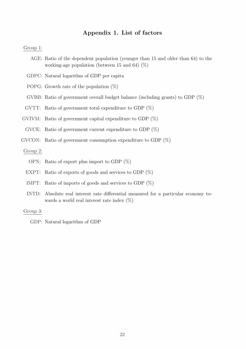
Appendix 1. List of factors
Group 1:
AGE: Ratio of the dependent population (younger than 15 and older than 64) to the
working-age population (between 15 and 64) (%)
GDPC: Natural logarithm of GDP per capita
POPG: Growth rate of the population (%)
GVBB: Ratio of government overall budget balance (including grants) to GDP (%)
GVTT: Ratio of government total expenditure to GDP (%)
GVIVM: Ratio of government capital expenditure to GDP (%)
GVCE: Ratio of government current expenditure to GDP (%)
GVCON: Ratio of government consumption expenditure to GDP (%)
Group 2:
OPN: Ratio of export plus import to GDP (%)
EXPT: Ratio of exports of goods and services to GDP (%)
IMPT: Ratio of imports of goods and services to GDP (%)
INTD: Absolute real interest rate differential measured for a particular economy to-
wards a world real interest rate index (%)
Group 3:
GDP: Natural logarithm of GDP
22

Appendix 2. List of countries included in W97
1 DZA-Algeria 33 DEU-Germany 65 NZL-New Zealand2 ARG-Argentina 34 GHA-Ghana 66 NER-Niger3 AUS-Australia 35 GRC-Greece 67 NGA-Nigeria4 AUT-Austria 36 GTM-Guatemala 68 NOR-Norway5 BGD-Bangladesh 37 GUY-Guyana 69 PAK-Pakistan6 BRB-Barbados 38 HTI-Haiti 70 PRY-Paraguay7 BEL-Belgium 39 HND-Honduras 71 PER-Peru8 BEN-Benin 40 HKG-Hong Kong, China 72 PHL-Philippines9 BWA-Botswana 41 HUN-Hungary 73 PRT-Portugal10 BRA-Brazil 42 ISL-Iceland 74 RWA-Rwanda11 BFA-Burkina Faso 43 IND-India 75 SAU-Saudi Arabia12 BDI-Burundi 44 IDN-Indonesia 76 SEN-Senegal13 CMR-Cameroon 45 IRL-Ireland 77 SGP-Singapore14 CAN-Canada 46 ISR-Israel 78 ZAF-South Africa15 CAF-Central African Republic 47 ITA-Italy 79 ESP-Spain16 CHL-Chile 48 JAM-Jamaica 80 LKA-Sri Lanka17 CHN-China 49 JPN-Japan 81 SUR-Suriname18 COL-Colombia 50 KEN-Kenya 82 SWZ-Swaziland19 ZAR-Congo, Dem. Rep. 51 KOR-Korea, Rep. 83 SWE-Sweden20 COG-Congo, Rep. 52 KWT-Kuwait 84 CHE-Switzerland21 CRI-Costa Rica 53 LUX-Luxembourg 85 SYR-Syrian Arab Republic22 CIV-Cote d’Ivoire 54 MDG-Madagascar 86 THA-Thailand23 DNK-Denmark 55 MWI-Malawi 87 TGO-Togo24 DOM-Dominican Republic 56 MYS-Malaysia 88 TTO-Trinidad and Tobago25 ECU-Ecuador 57 MLI-Mali 89 TUN-Tunisia26 EGY-Egypt, Arab Rep. 58 MLT-Malta 90 TUR-Turkey27 SLV-El Salvador 59 MRT-Mauritania 91 UGA-Uganda28 FJI-Fiji 60 MEX-Mexico 92 GBR-United Kingdom29 FIN-Finland 61 MAR-Morocco 93 USA-United States30 FRA-France 62 MMR-Myanmar 94 URY-Uruguay31 GAB-Gabon 63 NPL-Nepal 95 VEN-Venezuela, RB32 GMB-Gambia, The 64 NLD-Netherlands 96 ZMB-Zambia
97 ZWE-Zimbabwe
23
References
Abbott, A. and Vita, G. D. (2003). Another piece in the Feldstein-Horioka puzzle,
Scottish Journal of Political Economy 50: 69–89.
AmirKhalkhali, S., Dar, A. A. and AmirKhalkhali, S. (2003). Saving-investment
correlations, capital mobility and crowding out: some further results, Economic
Modelling 20: 1137–1149.
Artis, M. and Bayoumi, T. (1992). Global capital market integration and the current
account, in M. Taylor (ed.), Money and Financial Markets, Cambridge, MS and
Oxford: Blackwell, pp. 297–307.
Backus, D., Kehoe, P. and Kydland, F. (1992). International real business cycles,
Journal of Political Economy 100: 745–775.
Bajo-Rubio, O. (1998). The saving-investment correlation revisited: The case of
Spain, 1964-1994, Applied Economics Letters 5: 769–772.
Bernheim, B. D. (1987). Ricardian equivalence: An evaluation of theory and evidence,
NBER Macroeconomics Annual 1987, Cambridge, Mass.: MIT Press.
Blanchard, O. and Giavazzi, F. (2002). Current account deficits in the euro area.
the end of the feldstein horioka puzzle?, MIT Department of Economics Working
Paper 03-05.
Cai, Z., Fan, J. and Yao, Q. (2000). Functional-coefficient regression models for
nonlinear time series, Journal of the American Statistical Association 95: 941–
956.
Chinn, M. and Prasad, E. S. (2003). Medium-term determinants of current accounts
in industrial and developing countries: An empirical exploration, Journal of In-
ternational Economcis 59: 47–76.
Coakley, J., Fuertes, A.-M. and Spagnolo, F. (2004). Is the Feldstein-Horioka puzzle
history?, The Manchester School 72: 569–590.
Coakley, J., Kulasi, F. and Smith, R. (1996). Current account solvency and the
Feldstein-Horioka puzzle, Economic Journal 106: 620–627.
Coakley, J., Kulasi, F. and Smith, R. (1998). The Feldstein-Horioka puzzle and capital
mobility: A review, International Journal of Finance and Economics 3: 169–188.
Coiteux, M. and Olivier, S. (2000). The saving retention coefficient in the long run
and in the short run, Journal of International Money and Finance 19: 535–548.
Debelle, G. and Faruqee, H. (1996). What determines the current account? a cross-
sectional and panel approach, Technical Report 96/58, IMF Working Papers.
24

Edwards, S. (1995). Why are saving rates so different across countries?: An interna-
tional comparative analysis, NBER Working Paper 5097.
Feldstein, M. and Horioka, C. (1980). Domestic saving and international capital flows,
Economic Journal 90: 314–329.
Frankel, J. A. (1992). Measuring international capital mobility: A review, American
Economic Review 82(2): 197–202.
Freedman, D. A. (1981). Bootstrapping regression models, Annals of Statistics
9: 1218–1228.
French, K. and Poterba, J. (1991). Investor diversification and international equity
markets, American Economic Review 81: 222–226.
Gulley, O. D. (1992). Are saving and investment cointegrated?, Economics Letters
39: 55–58.
Haan, J. D. and Siermann, C. L. (1994). Saving, investment, and capital mobility. a
comment on Leachman, Open economies review 5: 5–17.
Hardle, W., Hall, P. and Marron, J. S. (1988). How far are automatically chosen
regression smoothing parameters from their optimum?, Journal of the American
Statistical Association 83: 86–99.
Herwartz, H. and Xu, F. (2006a). A new approach to bootstrap inference in functional
coefficient models, mimeo, Christian-Albrechts-University of Kiel.
Herwartz, H. and Xu, F. (2006b). Panel data model comparison for the investigation
of the saving-investment relation, Economics Working Paper 2006-06, Christian-
Albrechts-University of Kiel.
Herwartz, H. and Xu, F. (2006c). Reviewing the sustainability/stationarity of cur-
rent account imbalances with tests for bounded integration, Economics Working
Paper 2006-07, Christian-Albrechts-University of Kiel.
Ho, T.-W. (2002a). The Feldstein-Horioka puzzle revisited, Journal of International
Money and Finance 21: 555–564.
Ho, T.-W. (2002b). A panel cointegration approach to the investment-saving correla-
tion, Empirical Economics 27: 91–100.
Hodrick, R. J. and Prescott, E. C. (1997). Postwar u.s. business cycles: An empirical
investigation, Journal of Money, Credit and Banking 29: 1–16.
Jansen, W. J. (1996). Estimating saving-investment correlations: evidence for oecd
countries based on an error correction model, Journal of International Money
and Finance 15: 749–781.
Jansen, W. J. (1998). Interpreting saving-investment correlations, Open Economies
Review 9: 205–217.
25

Jansen, W. J. and Schulze, G. G. (1996). Theory-based measurement of the saving-
investment correlation with an application to norway, Economic Inquiry 34: 116–
132.
Kasuga, H. (2004). Saving-investment correlations in developing countries, Economics
Letters 83: 371–376.
Leachman, L. L. (1991). Saving, investment, and capital mobility among OECD
countries, Open economies review 2: 137–163.
Lemmen, J. J. and Eijffinger, S. C. (1995). The quantity approach to financial integra-
tion: The Feldstein-Horioka criterion revisited, Open economies review 6: 145–
165.
Masson, P. R., Bayoumi, T. and Samiei, H. (1998). International evidence on the
determinants of private saving, The World Bank Economic Review 12: 483–501.
Mendoza, E. G. (1991). Real business cycles in a small open economy, American
Economic Review 81: 797–818.
Milesi-Ferretti, G. M. and Razin, A. (1997). Sharp reductions in current account
deficits: An empirical analysis, NBER Working Paper 6310.
Milesi-Ferretti, G. M. and Razin, A. (1998). Current account reversals and currency
crises: Empirical regularities, NBER Working Paper 6620.
Miller, S. M. (1988). Are saving and investment cointegrated?, Economics Letters
27: 31–34.
Modigliani, F. (1970). The life-cycle hypothesis of saving and intercountry differences
in the saving ratio, in W. Eltis, M. Scorr and J. Wolfe (eds), Induction, Trade,
and Growth: Essays in Honour of Sir Roy Harrod, Clarendon Press, Oxford.
Modigliani, F. and Brumberg, R. (1954). Utility analysis and the consumption func-
tion: An interpretation of cross-section data, in K. K. Kurihara (ed.), Post-
Keynesian Economics, Rutgers University Press.
Moreno, R. (1997). Saving-investment dynamics and capital mobility in the Us and
Japan, Journal of International Money and Finance 16: 837–863.
Nadaraya, E. (1964). On estimating regression, Theory of Probability and its Appli-
cations 10: 186–190.
Obstfeld, M. (1986). Capital mobility in the world economy: Theory and measure-
ment, Carnegie-Rochester Conference Series on Public Policy 24: 55–104.
Obstfeld, M. and Rogoff, K. (2000). The six major puzzles in international macro-
economics: Is there a common cause?, in B. S. Bernanke and K. Rogoff (eds),
NBER Macroeconomics Anuual 2000, The MIT Press, pp. 339–390.
26

Ozmen, E. and Parmaksiz, K. (2003a). Exchange rate regimes and the Feldstein-
Horioka puzzle: The Freanch evidence, Applied Economics 35: 217–222.
Ozmen, E. and Parmaksiz, K. (2003b). Policy regime change and the Feldstein-
Horioka puzzle: The UK evidence, Journal of Policy Modeling 25: 137–149.
Pelagidis, T. and Mastroyiannis, T. (2003). The saving-investment correlation in
greece, 1960-1970: Implications for capital mobility, Journal of Policy Modeling
25: 609–616.
Pelgrin, F. and Schich, S. (2004). National saving-investment dynamics and interna-
tional capital mobility, Working Paper 2004-14, Bank of Canada.
Ravn, M. O. and Uhlig, H. (2002). On adjusting the HP-filter for the frequency of
observations, Review of Economics and Statistics 84: 371–380.
Sachsida, A. and Caetano, M. A.-R. (2000). The Feldstein-Horioka puzzle revisited,
Economics Letters 68: 85–88.
Schmidt, M. B. (2001). Savings and investment: Some international perspectives,
Sourthern Economic Journal 68: 446–456.
Scott, D. W. (1992). Multivariate Density Estimation: Theory, Practice, and Visual-
ization, John Wiley & Sons, New York, Chichester.
Sinha, T. and Sinha, D. (2004). The mother of all puzzles would not go away, Eco-
nomics Letters 82: 259–267.
Sinn, S. (1992). Saving-investment correlations and capital mobility: On the evidence
from annual data, Economic Journal 102: 1162–1170.
Summers, L. H. (1988). Tax policy and international competitiveness, in J. Frankel
(ed.), International Aspects of Fiscal Polices, Chicago: University of Chicago
Press, pp. 349–386.
Taylor, A. M. (1996). International capital mobility in history: The saving-investment
relationship, NBER Working Paper 5743.
Taylor, A. M. (1998). Argentina and the world capital market: Saving, investment,
and international capital mobility in the twentieth centruy, Journal of Develop-
ment Economics 57: 147–184.
Taylor, A. M. (2002). A century of current account dynamics, Journal of International
Money and Finance 21: 725–748.
Tesar, L. L. (1993). International rsik-sharing and non-traded goods, Journal of
International Economics 35: 69–89.
Vita, G. D. and Abbott, A. (2002). Are saving and investment cointegrated? an ardl
bounds testing approach, Economics Letters 77: 293–299.
Watson, G. (1964). Smooth regression analysis, Sankhya, Series A 26: 359–372.
27

Table 1: Between regression
I∗i = α + βS∗i + ei
Samples W97 L71 O26 O15 F16 E14 E11
Panel A: 1971 - 2002
β 0.43(11.24)
0.42(9.37)
0.59(5.11)
0.77(7.96)
0.62(4.44)
0.13(0.53)
−0.16(−0.71)
R2 0.57 0.56 0.52 0.83 0.58 0.02 0.05
Panel B: 1971 - 1986
β 0.44(9.44)
0.42(7.54)
0.69(6.58)
0.86(10.43)
0.66(4.50)
0.36(1.46)
0.18(0.78)
R2 0.48 0.45 0.64 0.89 0.59 0.15 0.06
Panel C: 1987 - 2002
β 0.38(9.96)
0.39(8.76)
0.39(3.27)
0.65(5.23)
0.30(2.24)
−0.02(−0.10)
−0.14(−0.90)
R2 0.51 0.53 0.31 0.68 0.26 0.00 0.08
This table reports slope estimates from the between regressions of the investment ratio on the savingratio. t-statistics appear in parentheses below the coefficient estimates. Coefficients which aresignificant at the 5% level are highlighted in bold face.
Table 2: Parametric factor dependence of the SI relation
γ1 in βi = γ0 + γ1wi + ui
Factor W97 L71 O26 O15 F16 E14 E11
AGE −0.006(−2.51)
0.001(0.15)
−0.026(−2.41)
−0.018(−1.48)
−0.052(−2.52)
−0.060(−2.26)
−0.068(−2.57)
OPN −0.004(−3.84)
−0.004(−3.41)
−0.005(−1.53)
0.000(0.06)
−0.006(−2.10)
−0.009(−2.68)
−0.009(−2.93)
EXPT −0.007(−3.53)
−0.007(−3.23)
−0.009(−1.54)
−0.000(−0.03)
−0.011(−2.04)
−0.016(−2.55)
−0.017(−2.68)
IMPT −0.009(−4.05)
−0.007(−3.50)
−0.010(−1.50)
0.002(0.16)
−0.012(−2.14)
−0.019(−2.79)
−0.020(−3.18)
t-critical value at 5% 1.985 1.994 2.064 2.131 2.145 2.179 2.262
OLS slope estimates for profile regressions (3). t-statistics appear in the parentheses below thecoefficient estimates. Coefficient estimates which are significant at the 5% level are highlighted inbold face. A list of abbreviations for the employed factor variables is given in the Appendix.
28

Table 3: Factor dependent model comparison
Factor W97 L71 O26 O15 F16 E14 E11
Group 1AGE 0.97 0.98 0.92 0.93 0.94 0.96 0.94GDPC 0.95 0.93 0.79 0.89 0.86 0.75 0.74POPG 0.99 1.00 0.98 0.91 0.95 0.91 0.93GVBB 0.99 0.99 0.96 0.97 0.92 0.96 1.02GVTT 0.96 0.96 0.91 0.91 0.87 0.87 0.86GVIVM 0.96 0.96 0.97 0.97 0.95 0.92 0.92GVCE 0.97 0.98 0.90 0.92 0.87 0.86 0.85GVCON 0.96 0.97 0.87 0.89 0.82 0.84 0.91
Group 2OPN 0.93 0.93 0.94 0.86 0.83 0.98 0.91EXPT 0.94 0.93 0.90 0.81 0.81 0.97 0.96IMPT 0.90 0.88 0.89 0.82 0.84 0.93 0.87INTD 1.01 1.00 1.00 1.04 0.98 1.00 1.02
Group 3GDP 0.95 0.98 0.89 0.92 0.74 0.75 0.78
This table reports CV criteria (absolute forecast errors) comparing of local estimates (12) againstthe factor invariant trivariate regression. Semiparametric CV estimates are given as a fraction of thepooled regression CV statistics.
29

1971 1980 1990 2002−0.5
0
0.5
1L71
1971 1980 1990 2002−1
−0.5
0
0.5
1
1.5
2O15
1971 1980 1990 2002−1
−0.5
0
0.5
1
1.5
2E11
Figure 1: Estimated time varying SI relations obtained from model (2) for the three non-overlappingcross sections. The solid line with stars shows the point estimates and the two dashed lines are thecorresponding 95% confidence intervals.
1971 1980 1990 20020
20
40
60
80
100
120
140
160
180
200
1971 1980 1990 200210
20
30
40
50
60
70
1971 1980 1990 2002−5
−4
−3
−2
−1
0
1
2
3
4
5
GermanyJapanUS
Germany
Japan
US
Figure 2: Dynamics of the openness ratio. The left hand side panel shows the observations for thecountries in O26 (dashed line) and the corresponding cross-sectional averages (solid line with stars).The medium panel displays the openness degree of Germany, the US and Japan (dashed line), andthe corresponding long run trend (solid line). The right hand side panel illustrates the deviationsfrom the long run trend for the given three countries.
30

−0.5
0
0.5
1E11
−1
0
1
2E11
0
0.5
1
1.5F16
−0.5
0
0.5
1F16
−1
0
1
2O26
0
0.5
1
1.5O26
−0.5
0
0.5
1L71
0
0.5
1L71
−2 −1 0 1 20
0.5
1
w(i)=v, w(t)=−1 ,0 ,1
W97
−2 −1 0 1 20
0.5
1
w(i)=0, w(t)=v
W97
−2
−1
0
1E11
−1
0
1F16
−2
−1
0
1O26
−0.5
0
0.5L71
−2 −1 0 1 2−0.5
0
0.5W97
Figure 3: Functional estimates of the SI relation conditional on the age dependency ratio for fiveselected cross sections. The left hand side panels show the estimated long run effects β(w(i) =0, w(t) = v) (solid). Dashed lines are the corresponding 95% confidence intervals. The mediumpanels display the short run effects for three local paths, i.e. β(w(i) = v, w(t) = 0) (circled line),β(w(i) = v, w(t) = −1) (solid) and β(w(i) = v, w(t) = 1) (dotted). The right hand side panels showthe difference between two estimated short run effects (solid), i.e. β(w(i) = v, w(t) = 1) − β(w(i) =v, w(t) = −1), and the corresponding 95% confidence intervals (dashed).
31

0
0.5
1
1.5GVBB: O26
−0.5
0
0.5
1GVBB: L71
−2 −1 0 1 2−0.5
0
0.5
1GVBB: W97
−0.5
0
0.5
1GVTT: W97
0
0.2
0.4
0.6
0.8GVIVM: W97
−0.5
0
0.5
1GVCE: W97
−2 −1 0 1 20
0.2
0.4
0.6
0.8GVCON: W97
Figure 4: Functional estimates of the SI relation conditional on fiscal variables. The long runeffects β(w(i) = 0, w(t) = v) are displayed. The solid line shows the point estimates and the dashedlines are the corresponding 95% confidence intervals.
32
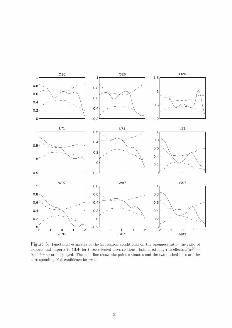
0
0.2
0.4
0.6
0.8
1O26
−0.5
0
0.5
1L71
−2 −1 0 1 20
0.2
0.4
0.6
0.8
1
OPN
W97
0.2
0.4
0.6
0.8
1O26
−0.2
0
0.2
0.4
0.6L71
−2 −1 0 1 2−0.2
0
0.2
0.4
0.6
0.8
EXPT
W97
0
0.5
1
1.5O26
0
0.2
0.4
0.6
0.8
1L71
−2 −1 0 1 20
0.2
0.4
0.6
0.8
1
IMPT
W97
Figure 5: Functional estimates of the SI relation conditional on the openness ratio, the ratio ofexports and imports to GDP for three selected cross sections. Estimated long run effects β(w(i) =0, w(t) = v) are displayed. The solid line shows the point estimates and the two dashed lines are thecorresponding 95% confidence intervals.
33

−2 −1 0 1 2−0.1
0
0.1
0.2
0.3
0.4
0.5
0.6GDPC
−2 −1 0 1 20
0.1
0.2
0.3
0.4
0.5
0.6
0.7POPG
−2 −1 0 1 20
0.1
0.2
0.3
0.4
0.5
0.6
0.7
0.8INTD
Figure 6: Functional estimates of the SI relation conditional on per capita income, the populationgrowth rate and the absolute real interest rate differential. Estimated long run effects β(w(i) =0, w(t) = v) are displayed for W97. The solid line shows the point estimates and the two dashed linesare the corresponding 95% confidence intervals.
−2 −1 0 1 2−0.2
−0.1
0
0.1
0.2
0.3
0.4
0.5
0.6
0.7E11
−2 −1 0 1 20.2
0.3
0.4
0.5
0.6
0.7
0.8
0.9
1O26
−2 −1 0 1 20.1
0.2
0.3
0.4
0.5
0.6
0.7
0.8
0.9W97
Figure 7: Functional estimates of the SI relation conditional on the logarithm of GDP. Estimatedlong run effects β(w(i) = 0, w(t) = v) are displayed. The solid line shows the point estimates and thetwo dashed lines are the corresponding 95% confidence intervals.
34