Embed Size (px)
Citation preview
In the Proceedings of the IEEE conference on Computer Vision and Pattern Recognition (CVPR), 2011
A fully automated greedy square jigsaw puzzle solver
Dolev Pomeranz Michal Shemesh Ohad Ben-Shahar
[email protected] [email protected] [email protected]
Computer Science Department, Ben-Gurion University of The Negev, Beer Sheva, Israel
Abstract
In the square jigsaw puzzle problem one is required to re-
construct the complete image from a set of non-overlapping,
unordered, square puzzle parts. Here we propose a fully au-
tomatic solver for this problem, where unlike some previous
work, it assumes no clues regarding parts’ location and re-
quires no prior knowledge about the original image or its
simplified (e.g., lower resolution) versions. To do so, we
introduce a greedy solver which combines both informed
piece placement and rearrangement of puzzle segments to
find the final solution. Among our other contributions are
new compatibility metrics which better predict the chances
of two given parts to be neighbors, and a novel estima-
tion measure which evaluates the quality of puzzle solutions
without the need for ground-truth information. Incorporat-
ing these contributions, our approach facilitates solutions
that surpass state-of-the-art solvers on puzzles of size larger
than ever attempted before.
1. Introduction
The popular jigsaw puzzle problem exists for many cen-
turies, long before it was first solved by a computer in
the 20th century. Given n jigsaw puzzle parts of an im-
age, it is required to reconstruct the complete image. Al-
though phrased as a game, this problem, which was proved
to be NP-complete [2, 7], serves a platform for many ap-
plications, e.g. in biological [14], molecular [22], text and
speech [12, 25], archaeological contexts [3, 10], and image
editing [4].
The traditional jigsaw puzzle problem assumes pieces of
various shapes, and indeed earlier computational work con-
sidered the problem in this form. The first jigsaw solver
proposed by Freeman and Garder in 1964 [8] was designed
to solve apictorial puzzles and was able to handle nine-piece
problems. By the end of the century, shaped-based solvers
were already able to reconstruct puzzles of more than 200
pieces [9]. The use of appearance and chromatic informa-
tion began only three decades after the work of Freeman
and Garder (e.g., [11, 6, 21, 24, 23, 13, 15]).
A major building block in most appearance-based puzzle
solvers evaluate the similarity between two parts, and the
strategies for doing so typically divide into two groups. One
approach compares the appearance of the abutting bound-
aries while using a formal distance measure between these
two vectors (e.g., [11, 6, 21, 24, 13, 15]). Alternatively, it
was suggested to use the entire part and measure its statis-
tical properties in order to group similar parts together [15]
or as a means to define pairwise similarity measures [11].
Once the similarity between two parts is estimated, differ-
ent classes of algorithms are employed to solve the puz-
zle, and in particular, previous methods have used greedy
algorithms [7, 15], dynamic programming [1], genetic al-
gorithms [21] and approximation algorithms on graphical
models [5].
Recently, Cho et al. [5] presented a probabilistic solver
which achieves approximated puzzle reconstruction via a
graphical model and a probability function that is maxi-
mized via loopy belief propagation. Since they lack a local
evidence term required for their graphical model, they em-
ployed two strategies that exploit prior knowledge - either
a dense-and-noisy evidence which estimates the low reso-
lution image from a bag of parts, or a sparse-and-accurate
evidence which assumes that a few parts, called “anchor
patches”, are given by an oracle (e.g., a human observer)
at their correct location in the puzzle. While only semi-
automatic, their approach was seminal in its ability to han-
dle puzzles with over 400 pieces.
In this paper we challenge the state-of-the-art in jigsaw
puzzle solving in several ways. We suggest a computational
framework that can handle in reasonable time square jigsaw
puzzles of size larger than ever attempted before. How-
ever, we completely exclude the use of clues, oracles, or
human intervention, as well as any use of prior knowledge
about the original image or simplified (e.g., lower resolu-
tion) versions of it. Despite these significant restrictions,
our approach achieves better than state-of-the-art perfor-
mance, and frequently succeeds in providing completely ac-
curate puzzle solutions.
9
Our puzzle solving framework is based on a greedy
solver, which works in several phases. First a compatibility
function is computed to measure the affinity between two
neighboring parts (as often done in other solvers as well).
Then the solver solves three problems - the placement prob-
lem, the segmentation problem, and the shifting problem.
The placement module places all parts on the board in an in-
formed fashion, the segmentation module identifies regions
which are likely to be assembled correctly, and the shift-
ing module relocates regions and parts to produce the final
result.
Our main contribution is a fully automated solver which
uses no clues, hints, or other prior knowledge whatsoever.
In addition, our contributions also include the proposal of
new and better compatibility metrics, as well as the intro-
duction of the concept of an estimation metric which evalu-
ates the quality of a given solution without any reference to
the original, ground-truth image. As we show, these metrics
become a critical tool that facilitates self evaluation in case
when no clues or prior knowledge are available. In what fol-
lows we first discuss these, as well as the rest of the metrics
involved in the solver.
2. Metrics
2.1. Compatibility Metrics
A compatibility metric is at the foundation of every jig-
saw solver. Given two puzzle parts xi, xj and a possible
spatial relation R between them, the compatibility function
predicts the likelihood that these two parts are indeed placed
as neighbors with relation R in the correct solution. With
R ∈ {l, r, u, d}, we use C(xi, xj , R) to denote the compat-
ibility that part xj is placed on either of the left, right, up,
or down side of part xi, respectively.
Optimally, one would wish to find a metric C such that
C(xi, xj , R) = 1 iff part xj is located to the R side of xi
in the original image and 0 otherwise. If such a function
exists, the jigsaw puzzle problem could be solved in poly-
nomial time by a greedy algorithm [7]. Motivated by the
above, we first discuss how one can measure the accuracy
of a compatibility function and then seek a compatibility
function C which is as accurate and discriminative as pos-
sible.
Measuring Compatibility Accuracy: In order to compare
between compatibility metrics, we denote the classification
criterion as the ratio between correct placements and the to-
tal number of possible placements. Similar to Cho et al. [5],
we define the correct placement of parts xi and xj accord-
ing to the compatibility metric C if part xj is in relation Rto part xi in the original image and if
∀xk ∈ Parts, C(xi, xj , R) ≥ C(xi, xk, R) . (1)
Recently, Cho et al. [5] evaluated five compatibility met-
rics, among which the dissimilarity-based compatibility
metric showed to be the most discriminative. Inspired by
both the dissimilarity-based metric and the characteristics
of natural images, we propose two new types of compatibil-
ity metrics, which will be described shortly after we review
the dissimilarity-based compatibility metric.
Dissimilarity-based Compatibility: The dissimilarity be-
tween two parts xi, xj can be measured by summing up the
squared color differences of the pixels along the parts’ abut-
ting boundaries [5]. For example, if we represent each color
image part in normalized LAB space by a K×K×3 matrix
(where K is the part width/height in pixels) then the dissim-
ilarity between parts xi and xj , where xj is to the right of
xi, can be defined as
D(xi, xj , r) =
K∑
k=1
3∑
d=1
(xi(k,K, d)− xj(k, 1, d))2 . (2)
We do emphasize that dissimilarity is not a distance mea-
sure, i.e., D(xj , xi, R) is not necessarily the same as (and
almost always different than) D(xi, xj , R).Although the dissimilarity-based metric was shown to be
the most discriminative among the tested metrics in Cho et
al. [5], the observation that it is related to the L2 norm of
the boundaries’ difference vector suggests that other norms
of the same difference vector could behave even better. In-
spired by the use of non Euclidean norms in image opera-
tions such as noise removal [19] or diffusion [20], and by
the observation that the L2 norm penalizes large boundary
differences very severely even though such large differences
do exist in natural images, we evaluated other Lp norms as
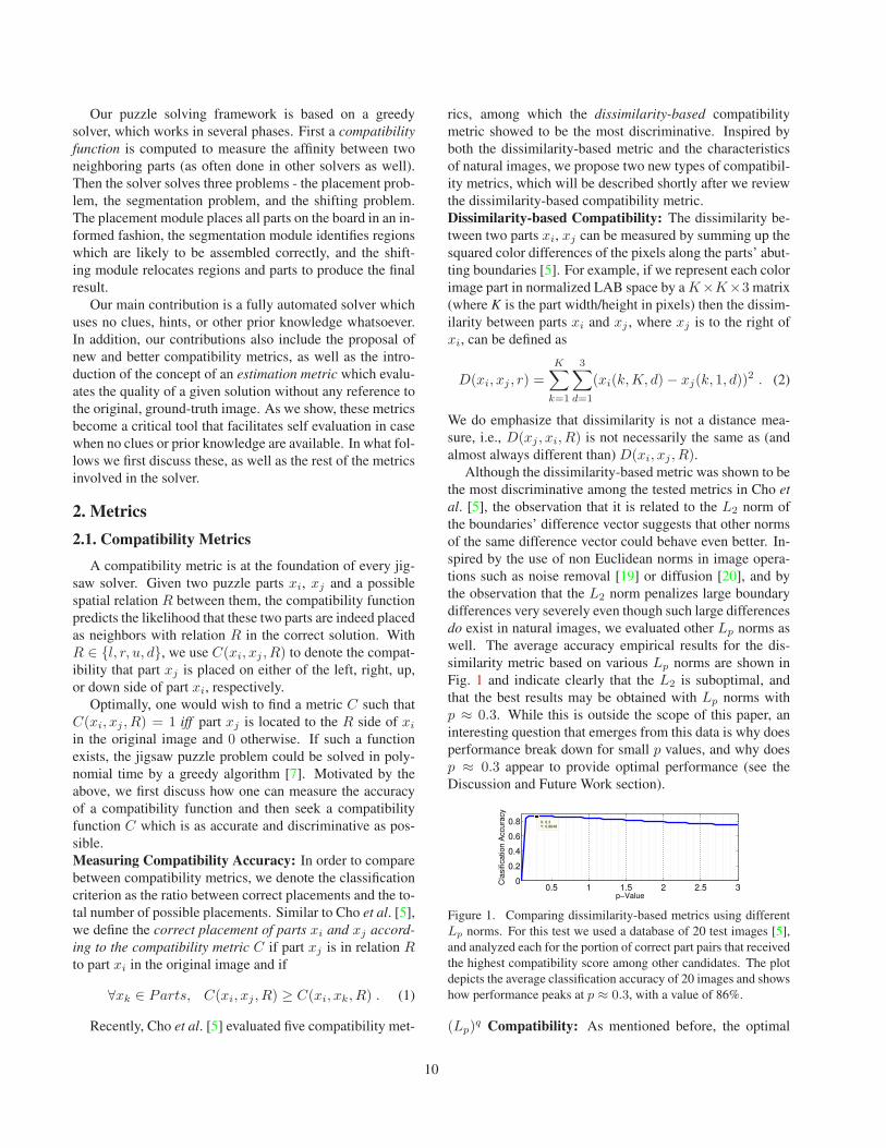
well. The average accuracy empirical results for the dis-
similarity metric based on various Lp norms are shown in
Fig. 1 and indicate clearly that the L2 is suboptimal, and
that the best results may be obtained with Lp norms with
p ≈ 0.3. While this is outside the scope of this paper, an
interesting question that emerges from this data is why does
performance break down for small p values, and why does
p ≈ 0.3 appear to provide optimal performance (see the
Discussion and Future Work section).
0.5 1 1.5 2 2.5 30
0.2
0.4
0.6
0.8 X: 0.3Y: 0.8648
p−Value
Cla
sific
atio
n A
ccu
racy
Figure 1. Comparing dissimilarity-based metrics using different
Lp norms. For this test we used a database of 20 test images [5],
and analyzed each for the portion of correct part pairs that received
the highest compatibility score among other candidates. The plot
depicts the average classification accuracy of 20 images and shows
how performance peaks at p ≈ 0.3, with a value of 86%.
(Lp)q Compatibility: As mentioned before, the optimal
10
compatibility function should also be as discriminative aspossible. In order to reflect the scattering of the dissimilar-ity values when obtaining their compatibility measures,wealso experimented with different powers q of the Lp norms.For example, the (Lp)
q compatibility for parts xi, xj wherexj is to the right of xi is defined as:
Dp,q(xi, xj , r) =
(
K∑
k=1
3∑
d=1
(|xi(k,K, d)− xj(k, 1, d)|)p
)
q
p
.
(3)
Having these dissimilarity values, we also propose to ob-
tain its compatibility measure slightly differently than done
previously. In particular, we define
C(xi, xj , R) ∝ exp
(
−Dp,q(xi, xj , R)
quartile(i, R)
)
, (4)
where quartile(i,R) is the quartile of the dissimilarity be-
tween all other parts in relation R to part xi. The quartile
normalization gives us valuable information about the scat-
tering of the compatibility function values, and in particular
emphasizes discriminative scattering.Although the value of q does not affect the dissimilarity
classification accuracy, it does have a significant effect onour solver’s performance. While Cho et al. [5] used p = 2and q = 2 in their dissimilarity metric (Eq. 2), we found thatoptimal results are achieved with power value q = 1/16 and
hence prefer to use a (Lp=3/10)q=1/16, i.e.,
Dp,q(xi, xj , r) =
(
K∑
k=1
3∑
d=1
(|xi(k,K, d)− xj(k, 1, d)|)3
10
)5
24
.
(5)
Prediction-based Compatibility: While dissimilarity-
based metrics may be improved greatly by employing (Lp)q
affinities, other possibilities may be promising as well. In
particular, as opposed to measure differences, one may at-
tempt to quantify how well one can predict the boundary
content of one part based on the boundary content of the
other. The better the prediction, the higher the compatibil-
ity of the two parts, a measure we call a Prediction-based
Compatibility.Naturally, predictions over the boundaries can be made
using Taylor’s expansion. A first order prediction wouldneed an estimation of the derivative of each part at itsboundary, a computation that can be done numerically inone of several ways. For example, employing backwarddifferences estimation using the last two pixels in each rownear the boundary, one can obtain a prediction of the firstpixel in the neighboring part. The quality of this predictioncan then be verified against the actual pixel value from thesecond part by using any desired norm, and in general, us-ing (Lp)
q for preselected p and q as discussed above in thedissimilarity measure. Importantly, we repeat this computa-tion for both parts in a symmetric fashion. For example, theprediction metric for two parts xi, xj with relation r when
using (Lp)q with p = 3/10 and q = 1/16 can be expressed
by the following expression
Pred(xi, xj , r) =∑K
k=1
∑
3
d=1[
([2xi(k,K, d)− xi(k,K − 1, d)]− xj(k, 1, d))3
10+
([2xj(k, 1, d)− xj(k, 2, d)]− xi(k,K, d))3
10
] 5
24
(6)
and obtain its compatibility measure as in Eq. 4.
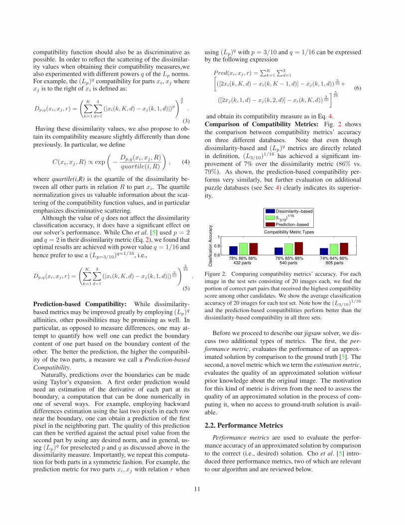
Comparison of Compatibility Metrics: Fig. 2 shows
the comparison between compatibility metrics’ accuracy
on three different databases. Note that even though
dissimilarity-based and (Lp)q metrics are directly related
in definition, (L3/10)1/16 has achieved a significant im-
provement of 7% over the dissimilarity metric (86% vs.
79%). As shown, the prediction-based compatibility per-
forms very similarly, but further evaluation on additional
puzzle databases (see Sec 4) clearly indicates its superior-
ity.
78% 86% 86% 76% 85% 88% 74% 84% 86%0.6
0.8
1Compatibility Metric Types
432 parts 540 parts 805 parts
Cla
sific
ation A
ccura
cy
Dissimilarity−based
(L3/10
)1/16
Prediction−based
Figure 2. Comparing compatibility metrics’ accuracy. For each
image in the test sets consisting of 20 images each, we find the
portion of correct part pairs that received the highest compatibility
score among other candidates. We show the average classification
accuracy of 20 images for each test set. Note how the (L3/10)1/16
and the prediction-based compatibilities perform better than the
dissimilarity-based compatibility in all three sets.
Before we proceed to describe our jigsaw solver, we dis-
cuss two additional types of metrics. The first, the per-
formance metric, evaluates the performance of an approx-
imated solution by comparison to the ground truth [5]. The
second, a novel metric which we term the estimation metric,
evaluates the quality of an approximated solution without
prior knowledge about the original image. The motivation
for this kind of metric is driven from the need to assess the
quality of an approximated solution in the process of com-
puting it, when no access to ground-truth solution is avail-
able.
2.2. Performance Metrics
Performance metrics are used to evaluate the perfor-
mance accuracy of an approximated solution by comparison
to the correct (i.e., desired) solution. Cho et al. [5] intro-
duced three performance metrics, two of which are relevant
to our algorithm and are reviewed below.
11
Direct Comparison Metric: The direct comparison met-
ric calculates the ratio between the number of parts in the
approximated solution which are placed in their correct lo-
cation and the total number of parts [5].
Neighbor Comparison Metric: The neighbor comparison
metric calculates the ratio between the number of correct
neighbors placement for each part and the total number of
neighbors [5].
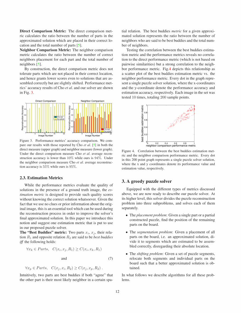
By construction, the direct comparison metric does not
tolerate parts which are not placed in their correct location,
and hence grants lower scores even to solutions that are as-
sembled correctly but are slightly shifted. Performance met-
rics’ accuracy results of Cho et al. and our solver are shown
in Fig. 3.
5 10 15 200
0.2
0.4
0.6
0.8
1
Diriect Comparison
Image Number
Reconstr
uction A
ccura
cy
Cho etal
Our solver
5 10 15 200
0.2
0.4
0.6
0.8
1
Neighbor Comparison
Image Number
Reconstr
uction A
ccura
cy
Cho etal
Our solver
Figure 3. Performance metrics’ accuracy comparison. We com-
pare our results with those reported by Cho et al. [5] in both the
direct measure (upper graph) and neighbor measure (lower graph).
Under the direct comparison measure Cho et al. average recon-
struction accuracy is lower than 10% while ours is 94%. Under
the neighbor comparison measure Cho et al. average reconstruc-
tion accuracy is 55% while ours is 95%.
2.3. Estimation Metrics
While the performance metrics evaluate the quality of
solutions in the presence of a ground truth image, the es-
timation metric is designed to provide such quality scores
without knowing the correct solution whatsoever. Given the
fact that we use no clues or prior information about the orig-
inal image, this is an essential tool which can be used during
the reconstruction process in order to improve the solver’s
final approximated solution. In this paper we introduce this
notion and suggest one estimation metric that is put to use
in our proposed puzzle solver.
The “Best Buddies” metric: Two parts xi, xj , their rela-
tion R1 and opposite relation R2 are said to be best buddies
iff the following holds:
∀xk ∈ Parts, C(xi, xj , R1) ≥ C(xi, xk, R1)
and
∀xp ∈ Parts, C(xj , xi, R2) ≥ C(xj , xp, R2) .
(7)
Intuitively, two parts are best buddies if both “agree” that
the other part is their most likely neighbor in a certain spa-
tial relation. The best buddies metric for a given approxi-
mated solution represents the ratio between the number of
neighbors who are said to be best buddies and the total num-
ber of neighbors.
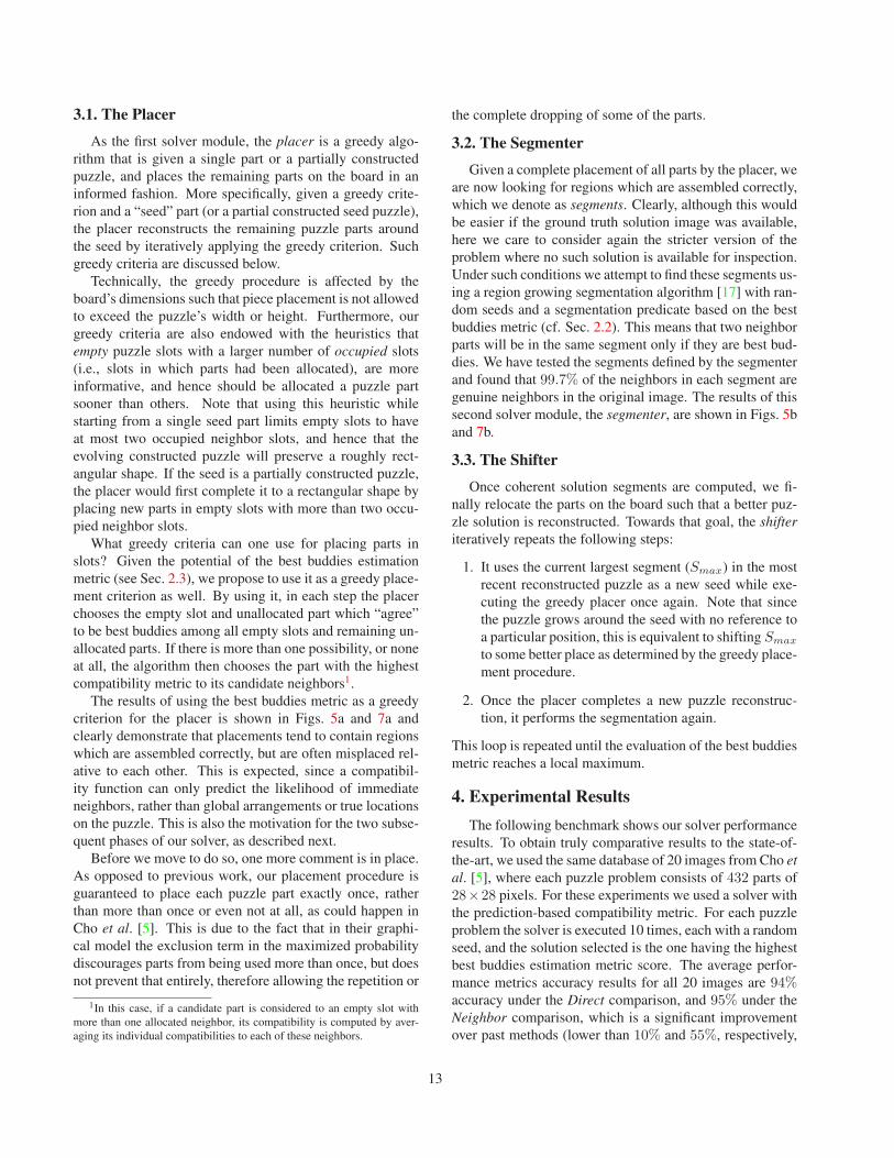
Testing the correlation between the best buddies estima-
tion metric and the performance metrics reveals no correla-
tion to the direct performance metric (which is not based on
pairwise similarities) but a strong correlation to the neigh-
bor performance metric. Fig.4 depicts this relationship as
a scatter plot of the best buddies estimation metric vs. the
neighbor performance metric. Every dot in the graph repre-
sent a single puzzle solver solution, where the x-coordinates
and the y-coordinate denote the performance accuracy and
estimation accuracy, respectively. Each image in the set was
tested 10 times, totaling 200 sample points.
0 0.2 0.4 0.6 0.8 10
0.2
0.4
0.6
0.8
1
neighbor comparison performance metricbest buddie
s e
stim
ation m
etr
ic
Figure 4. Correlation between the best buddies estimation met-
ric and the neighbor comparison performance metric. Every dot
in this 200 point graph represents a single puzzle solver solution,
where the x and y coordinates denote its performance value and
estimation value, respectively.
3. A greedy puzzle solver
Equipped with the different types of metrics discussed
above, we are now ready to describe our puzzle solver. At
its higher level, this solver divides the puzzle reconstruction
problem into three subproblems, and solves each of them
separately.
• The placement problem: Given a single part or a partial
constructed puzzle, find the position of the remaining
parts on the board.
• The segmentation problem: Given a placement of all
parts on the board, i.e. an approximated solution, di-
vide it to segments which are estimated to be assem-
bled correctly, disregarding their absolute location.
• The shifting problem: Given a set of puzzle segments,
relocate both segments and individual parts on the
board such that a better approximated solution is ob-
tained.
In what follows we describe algorithms for all these prob-
lems.
12
3.1. The Placer
As the first solver module, the placer is a greedy algo-
rithm that is given a single part or a partially constructed
puzzle, and places the remaining parts on the board in an
informed fashion. More specifically, given a greedy crite-
rion and a “seed” part (or a partial constructed seed puzzle),
the placer reconstructs the remaining puzzle parts around
the seed by iteratively applying the greedy criterion. Such
greedy criteria are discussed below.
Technically, the greedy procedure is affected by the
board’s dimensions such that piece placement is not allowed
to exceed the puzzle’s width or height. Furthermore, our
greedy criteria are also endowed with the heuristics that
empty puzzle slots with a larger number of occupied slots
(i.e., slots in which parts had been allocated), are more
informative, and hence should be allocated a puzzle part
sooner than others. Note that using this heuristic while
starting from a single seed part limits empty slots to have
at most two occupied neighbor slots, and hence that the
evolving constructed puzzle will preserve a roughly rect-
angular shape. If the seed is a partially constructed puzzle,
the placer would first complete it to a rectangular shape by
placing new parts in empty slots with more than two occu-
pied neighbor slots.
What greedy criteria can one use for placing parts in
slots? Given the potential of the best buddies estimation
metric (see Sec. 2.3), we propose to use it as a greedy place-
ment criterion as well. By using it, in each step the placer
chooses the empty slot and unallocated part which “agree”
to be best buddies among all empty slots and remaining un-
allocated parts. If there is more than one possibility, or none
at all, the algorithm then chooses the part with the highest
compatibility metric to its candidate neighbors1.
The results of using the best buddies metric as a greedy
criterion for the placer is shown in Figs. 5a and 7a and
clearly demonstrate that placements tend to contain regions
which are assembled correctly, but are often misplaced rel-
ative to each other. This is expected, since a compatibil-
ity function can only predict the likelihood of immediate
neighbors, rather than global arrangements or true locations
on the puzzle. This is also the motivation for the two subse-
quent phases of our solver, as described next.
Before we move to do so, one more comment is in place.
As opposed to previous work, our placement procedure is
guaranteed to place each puzzle part exactly once, rather
than more than once or even not at all, as could happen in
Cho et al. [5]. This is due to the fact that in their graphi-
cal model the exclusion term in the maximized probability
discourages parts from being used more than once, but does
not prevent that entirely, therefore allowing the repetition or
1In this case, if a candidate part is considered to an empty slot with
more than one allocated neighbor, its compatibility is computed by aver-
aging its individual compatibilities to each of these neighbors.
the complete dropping of some of the parts.
3.2. The Segmenter
Given a complete placement of all parts by the placer, we
are now looking for regions which are assembled correctly,
which we denote as segments. Clearly, although this would
be easier if the ground truth solution image was available,
here we care to consider again the stricter version of the
problem where no such solution is available for inspection.
Under such conditions we attempt to find these segments us-
ing a region growing segmentation algorithm [17] with ran-
dom seeds and a segmentation predicate based on the best
buddies metric (cf. Sec. 2.2). This means that two neighbor
parts will be in the same segment only if they are best bud-
dies. We have tested the segments defined by the segmenter
and found that 99.7% of the neighbors in each segment are
genuine neighbors in the original image. The results of this
second solver module, the segmenter, are shown in Figs. 5b
and 7b.
3.3. The Shifter
Once coherent solution segments are computed, we fi-
nally relocate the parts on the board such that a better puz-
zle solution is reconstructed. Towards that goal, the shifter
iteratively repeats the following steps:
1. It uses the current largest segment (Smax) in the most
recent reconstructed puzzle as a new seed while exe-
cuting the greedy placer once again. Note that since
the puzzle grows around the seed with no reference to
a particular position, this is equivalent to shifting Smax
to some better place as determined by the greedy place-
ment procedure.
2. Once the placer completes a new puzzle reconstruc-
tion, it performs the segmentation again.
This loop is repeated until the evaluation of the best buddies
metric reaches a local maximum.
4. Experimental Results
The following benchmark shows our solver performance
results. To obtain truly comparative results to the state-of-
the-art, we used the same database of 20 images from Cho et
al. [5], where each puzzle problem consists of 432 parts of
28×28 pixels. For these experiments we used a solver with
the prediction-based compatibility metric. For each puzzle
problem the solver is executed 10 times, each with a random
seed, and the solution selected is the one having the highest
best buddies estimation metric score. The average perfor-
mance metrics accuracy results for all 20 images are 94%accuracy under the Direct comparison, and 95% under the
Neighbor comparison, which is a significant improvement
over past methods (lower than 10% and 55%, respectively,
13
placer results segmenter results final solution
(2-a) (2-b) (2-c)
(3-a) (3-b) (3-c)
Original Image
Image 2
Image 3
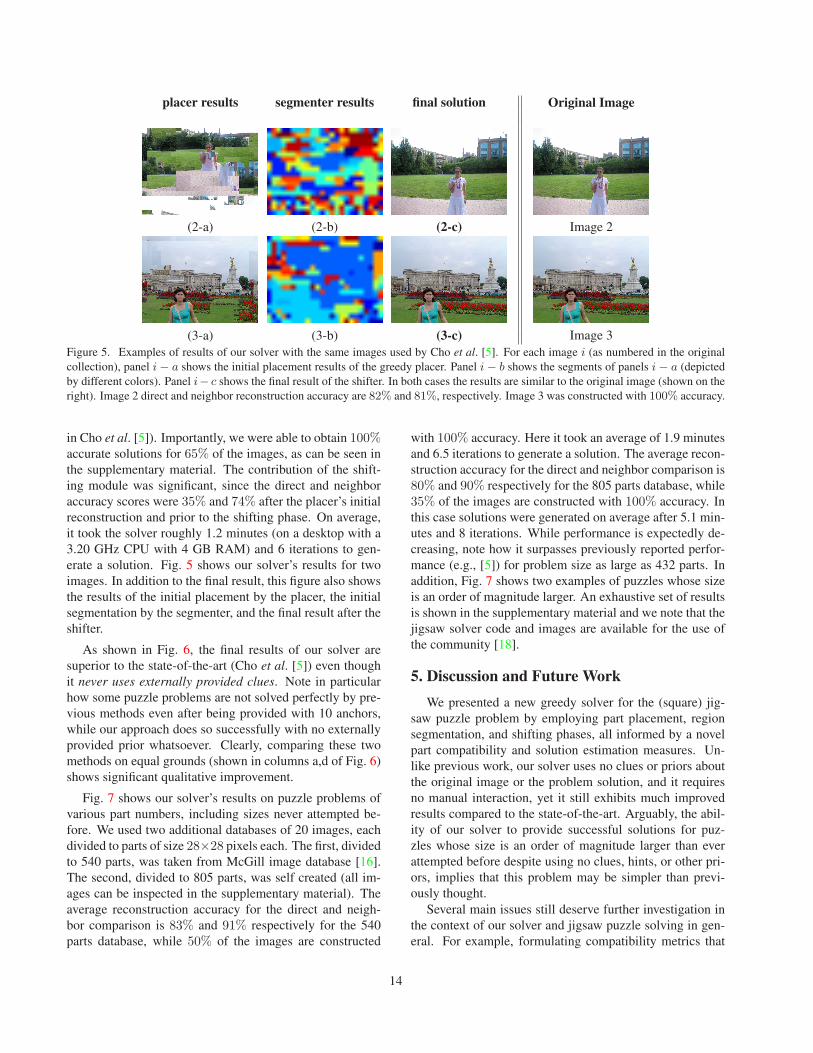
Figure 5. Examples of results of our solver with the same images used by Cho et al. [5]. For each image i (as numbered in the original
collection), panel i− a shows the initial placement results of the greedy placer. Panel i− b shows the segments of panels i− a (depicted
by different colors). Panel i− c shows the final result of the shifter. In both cases the results are similar to the original image (shown on the
right). Image 2 direct and neighbor reconstruction accuracy are 82% and 81%, respectively. Image 3 was constructed with 100% accuracy.
in Cho et al. [5]). Importantly, we were able to obtain 100%accurate solutions for 65% of the images, as can be seen in
the supplementary material. The contribution of the shift-
ing module was significant, since the direct and neighbor
accuracy scores were 35% and 74% after the placer’s initial
reconstruction and prior to the shifting phase. On average,
it took the solver roughly 1.2 minutes (on a desktop with a
3.20 GHz CPU with 4 GB RAM) and 6 iterations to gen-
erate a solution. Fig. 5 shows our solver’s results for two
images. In addition to the final result, this figure also shows
the results of the initial placement by the placer, the initial
segmentation by the segmenter, and the final result after the
shifter.
As shown in Fig. 6, the final results of our solver are
superior to the state-of-the-art (Cho et al. [5]) even though
it never uses externally provided clues. Note in particular
how some puzzle problems are not solved perfectly by pre-
vious methods even after being provided with 10 anchors,
while our approach does so successfully with no externally
provided prior whatsoever. Clearly, comparing these two
methods on equal grounds (shown in columns a,d of Fig. 6)
shows significant qualitative improvement.
Fig. 7 shows our solver’s results on puzzle problems of
various part numbers, including sizes never attempted be-
fore. We used two additional databases of 20 images, each
divided to parts of size 28×28 pixels each. The first, divided
to 540 parts, was taken from McGill image database [16].
The second, divided to 805 parts, was self created (all im-
ages can be inspected in the supplementary material). The
average reconstruction accuracy for the direct and neigh-
bor comparison is 83% and 91% respectively for the 540
parts database, while 50% of the images are constructed
with 100% accuracy. Here it took an average of 1.9 minutes
and 6.5 iterations to generate a solution. The average recon-
struction accuracy for the direct and neighbor comparison is
80% and 90% respectively for the 805 parts database, while
35% of the images are constructed with 100% accuracy. In
this case solutions were generated on average after 5.1 min-
utes and 8 iterations. While performance is expectedly de-
creasing, note how it surpasses previously reported perfor-
mance (e.g., [5]) for problem size as large as 432 parts. In
addition, Fig. 7 shows two examples of puzzles whose size
is an order of magnitude larger. An exhaustive set of results
is shown in the supplementary material and we note that the
jigsaw solver code and images are available for the use of
the community [18].
5. Discussion and Future Work
We presented a new greedy solver for the (square) jig-
saw puzzle problem by employing part placement, region
segmentation, and shifting phases, all informed by a novel
part compatibility and solution estimation measures. Un-
like previous work, our solver uses no clues or priors about
the original image or the problem solution, and it requires
no manual interaction, yet it still exhibits much improved
results compared to the state-of-the-art. Arguably, the abil-
ity of our solver to provide successful solutions for puz-
zles whose size is an order of magnitude larger than ever
attempted before despite using no clues, hints, or other pri-
ors, implies that this problem may be simpler than previ-
ously thought.
Several main issues still deserve further investigation in
the context of our solver and jigsaw puzzle solving in gen-
eral. For example, formulating compatibility metrics that
14
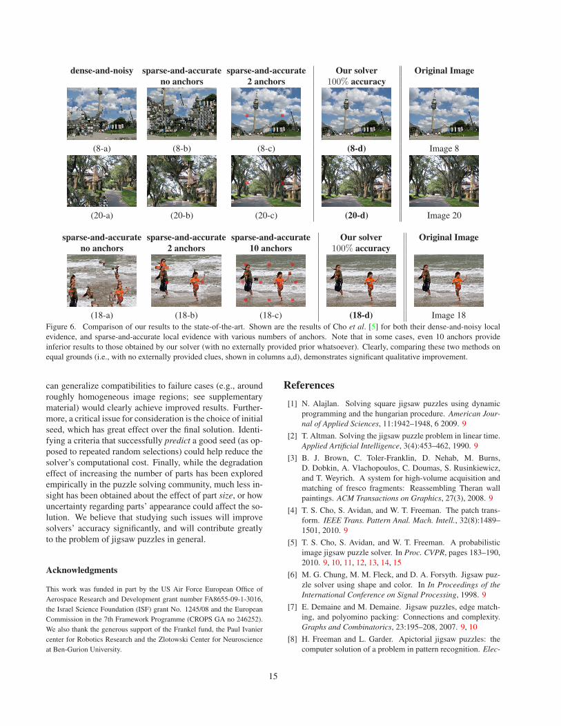
dense-and-noisy sparse-and-accurate sparse-and-accurate Our solver Original Image
no anchors 2 anchors 100% accuracy
(8-a) (8-b) (8-c) (8-d) Image 8
(20-a) (20-b) (20-c) (20-d) Image 20
sparse-and-accurate sparse-and-accurate sparse-and-accurate Our solver Original Image
no anchors 2 anchors 10 anchors 100% accuracy
(18-a) (18-b) (18-c) (18-d) Image 18
Figure 6. Comparison of our results to the state-of-the-art. Shown are the results of Cho et al. [5] for both their dense-and-noisy local
evidence, and sparse-and-accurate local evidence with various numbers of anchors. Note that in some cases, even 10 anchors provide
inferior results to those obtained by our solver (with no externally provided prior whatsoever). Clearly, comparing these two methods on
equal grounds (i.e., with no externally provided clues, shown in columns a,d), demonstrates significant qualitative improvement.
can generalize compatibilities to failure cases (e.g., around
roughly homogeneous image regions; see supplementary
material) would clearly achieve improved results. Further-
more, a critical issue for consideration is the choice of initial
seed, which has great effect over the final solution. Identi-
fying a criteria that successfully predict a good seed (as op-
posed to repeated random selections) could help reduce the
solver’s computational cost. Finally, while the degradation
effect of increasing the number of parts has been explored
empirically in the puzzle solving community, much less in-
sight has been obtained about the effect of part size, or how
uncertainty regarding parts’ appearance could affect the so-
lution. We believe that studying such issues will improve
solvers’ accuracy significantly, and will contribute greatly
to the problem of jigsaw puzzles in general.
Acknowledgments
This work was funded in part by the US Air Force European Office of
Aerospace Research and Development grant number FA8655-09-1-3016,
the Israel Science Foundation (ISF) grant No. 1245/08 and the European
Commission in the 7th Framework Programme (CROPS GA no 246252).
We also thank the generous support of the Frankel fund, the Paul Ivanier
center for Robotics Research and the Zlotowski Center for Neuroscience
at Ben-Gurion University.
References
[1] N. Alajlan. Solving square jigsaw puzzles using dynamic
programming and the hungarian procedure. American Jour-
nal of Applied Sciences, 11:1942–1948, 6 2009. 9
[2] T. Altman. Solving the jigsaw puzzle problem in linear time.
Applied Artificial Intelligence, 3(4):453–462, 1990. 9
[3] B. J. Brown, C. Toler-Franklin, D. Nehab, M. Burns,
D. Dobkin, A. Vlachopoulos, C. Doumas, S. Rusinkiewicz,
and T. Weyrich. A system for high-volume acquisition and
matching of fresco fragments: Reassembling Theran wall
paintings. ACM Transactions on Graphics, 27(3), 2008. 9
[4] T. S. Cho, S. Avidan, and W. T. Freeman. The patch trans-
form. IEEE Trans. Pattern Anal. Mach. Intell., 32(8):1489–
1501, 2010. 9
[5] T. S. Cho, S. Avidan, and W. T. Freeman. A probabilistic
image jigsaw puzzle solver. In Proc. CVPR, pages 183–190,
2010. 9, 10, 11, 12, 13, 14, 15
[6] M. G. Chung, M. M. Fleck, and D. A. Forsyth. Jigsaw puz-
zle solver using shape and color. In In Proceedings of the
International Conference on Signal Processing, 1998. 9
[7] E. Demaine and M. Demaine. Jigsaw puzzles, edge match-
ing, and polyomino packing: Connections and complexity.
Graphs and Combinatorics, 23:195–208, 2007. 9, 10
[8] H. Freeman and L. Garder. Apictorial jigsaw puzzles: the
computer solution of a problem in pattern recognition. Elec-
15
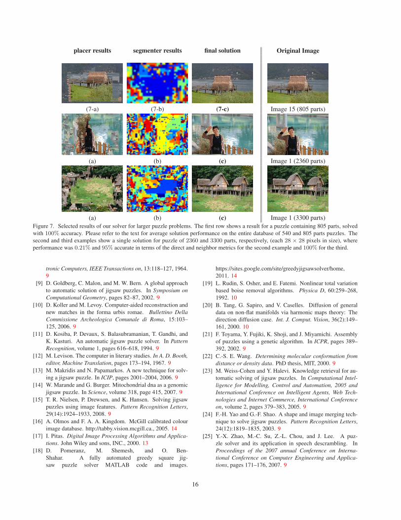
placer results segmenter results final solution
(7-a) (7-b) (7-c)
(a) (b) (c)
(a) (b) (c)
Original Image
Image 15 (805 parts)
Image 1 (2360 parts)
Image 1 (3300 parts)
Figure 7. Selected results of our solver for larger puzzle problems. The first row shows a result for a puzzle containing 805 parts, solved
with 100% accuracy. Please refer to the text for average solution performance on the entire database of 540 and 805 parts puzzles. The
second and third examples show a single solution for puzzle of 2360 and 3300 parts, respectively, (each 28 × 28 pixels in size), where
performance was 0.21% and 95% accurate in terms of the direct and neighbor metrics for the second example and 100% for the third.
tronic Computers, IEEE Transactions on, 13:118–127, 1964.
9
[9] D. Goldberg, C. Malon, and M. W. Bern. A global approach
to automatic solution of jigsaw puzzles. In Symposium on
Computational Geometry, pages 82–87, 2002. 9
[10] D. Koller and M. Levoy. Computer-aided reconstruction and
new matches in the forma urbis romae. Bullettino Della
Commissione Archeologica Comunale di Roma, 15:103–
125, 2006. 9
[11] D. Kosiba, P. Devaux, S. Balasubramanian, T. Gandhi, and
K. Kasturi. An automatic jigsaw puzzle solver. In Pattern
Recognition, volume 1, pages 616–618, 1994. 9
[12] M. Levison. The computer in literary studies. In A. D. Booth,
editor, Machine Translation, pages 173–194, 1967. 9
[13] M. Makridis and N. Papamarkos. A new technique for solv-
ing a jigsaw puzzle. In ICIP, pages 2001–2004, 2006. 9
[14] W. Marande and G. Burger. Mitochondrial dna as a genomic
jigsaw puzzle. In Science, volume 318, page 415, 2007. 9
[15] T. R. Nielsen, P. Drewsen, and K. Hansen. Solving jigsaw
puzzles using image features. Pattern Recognition Letters,
29(14):1924–1933, 2008. 9
[16] A. Olmos and F. A. A. Kingdom. McGill calibrated colour
image database. http://tabby.vision.mcgill.ca., 2005. 14
[17] I. Pitas. Digital Image Processing Algorithms and Applica-
tions. John Wiley and sons, INC., 2000. 13
[18] D. Pomeranz, M. Shemesh, and O. Ben-
Shahar. A fully automated greedy square jig-
saw puzzle solver MATLAB code and images.
https://sites.google.com/site/greedyjigsawsolver/home,
2011. 14
[19] L. Rudin, S. Osher, and E. Fatemi. Nonlinear total variation
based boise removal algorithms. Physica D, 60:259–268,
1992. 10
[20] B. Tang, G. Sapiro, and V. Caselles. Diffusion of general
data on non-flat manifolds via harmonic maps theory: The
direction diffusion case. Int. J. Comput. Vision, 36(2):149–
161, 2000. 10
[21] F. Toyama, Y. Fujiki, K. Shoji, and J. Miyamichi. Assembly
of puzzles using a genetic algorithm. In ICPR, pages 389–
392, 2002. 9
[22] C.-S. E. Wang. Determining molecular conformation from
distance or density data. PhD thesis, MIT, 2000. 9
[23] M. Weiss-Cohen and Y. Halevi. Knowledge retrieval for au-
tomatic solving of jigsaw puzzles. In Computational Intel-
ligence for Modelling, Control and Automation, 2005 and
International Conference on Intelligent Agents, Web Tech-
nologies and Internet Commerce, International Conference
on, volume 2, pages 379–383, 2005. 9
[24] F.-H. Yao and G.-F. Shao. A shape and image merging tech-
nique to solve jigsaw puzzles. Pattern Recognition Letters,
24(12):1819–1835, 2003. 9
[25] Y.-X. Zhao, M.-C. Su, Z.-L. Chou, and J. Lee. A puz-
zle solver and its application in speech descrambling. In
Proceedings of the 2007 annual Conference on Interna-
tional Conference on Computer Engineering and Applica-
tions, pages 171–176, 2007. 9
16