A framework of traveling companion discovery on trajectory data streams

3

A Framework of Traveling Companion Discovery on TrajectoryData Streams

LU-AN TANG, University of Illinois at Urbana-Champaign and Microsoft Research AsiaYU ZHENG and JING YUAN, Microsoft Research AsiaJIAWEI HAN, University of Illinois at Urbana-ChampaignALICE LEUNG, BBN TechnologiesWEN-CHIH PENG, National Chiao Tung UniversityTHOMAS LA PORTA, Pennsylvania State University

The advance of mobile technologies leads to huge volumes of spatio-temporal data collected in the form oftrajectory data streams. In this study, we investigate the problem of discovering object groups that traveltogether (i.e., traveling companions) from trajectory data streams. Such technique has broad applications inthe areas of scientific study, transportation management, and military surveillance. To discover travelingcompanions, the monitoring system should cluster the objects of each snapshot and intersect the clusteringresults to retrieve moving-together objects. Since both clustering and intersection steps involve high com-putational overhead, the key issue of companion discovery is to improve the efficiency of algorithms. Wepropose the models of closed companion candidates and smart intersection to accelerate data processing. Adata structure termed traveling buddy is designed to facilitate scalable and flexible companion discoveryfrom trajectory streams. The traveling buddies are microgroups of objects that are tightly bound together.By only storing the object relationships rather than their spatial coordinates, the buddies can be dynam-ically maintained along the trajectory stream with low cost. Based on traveling buddies, the system candiscover companions without accessing the object details. In addition, we extend the proposed framework todiscover companions on more complicated scenarios with spatial and temporal constraints, such as on theroad network and battlefield. The proposed methods are evaluated with extensive experiments on both realand synthetic datasets. Experimental results show that our proposed buddy-based approach is an order ofmagnitude faster than the baselines and achieves higher accuracy in companion discovery.

Categories and Subject Descriptors: H.2.8 [Database Applications]: Data Mining

General Terms: Algorithms, Experimentation, Performance

Additional Key Words and Phrases: Trajectory, data stream, clustering

L.-A. Tang is currently affiliated with NEC Labs America.The work was supported in part by U.S. NSF grants IIS-0905215, CNS-0931975, CCF-0905014, IIS-1017362,the U.S. Army Research Laboratory under Cooperative Agreement no. W911NF-09-2-0053 (NS-CTA). Theviews and conclusions contained in this document are those of the authors and should not be interpreted asrepresenting the official policies, either expressed or implied, of the Army Research Laboratory or the U.S.Government.Authors’ addresses: L.-A. Tang (corresponding author), University of Illinois at Urbana-Champaign, 601 EJohn St, Champaign, IL 61820; email: [email protected]; Y. Zheng and J. Yuan, Microsoft ResearchAsia; J. Han, University of Illinois at Urbana-Champaign, 601 E John St, Champaign, IL 61820; A. Leung,BBN Technologies; W.-C. Peng, National Chiao Tung University, 300, Taiwan, Hsinchu City, Dong District,Taiwan, ROC; T. La Porta, Pennsylvania State University, 201 Old Main, University Park PA 16802.Permission to make digital or hard copies of part or all of this work for personal or classroom use is grantedwithout fee provided that copies are not made or distributed for profit or commercial advantage and thatcopies show this notice on the first page or initial screen of a display along with the full citation. Copyrights forcomponents of this work owned by others than ACM must be honored. Abstracting with credit is permitted.To copy otherwise, to republish, to post on servers, to redistribute to lists, or to use any component of thiswork in other works requires prior specific permission and/or a fee. Permissions may be requested fromPublications Dept., ACM, Inc., 2 Penn Plaza, Suite 701, New York, NY 10121-0701 USA, fax +1 (212)869-0481, or [email protected]© 2013 ACM 2157-6904/2013/12-ART3 $15.00DOI: http://dx.doi.org/10.1145/2542182.2542185

ACM Transactions on Intelligent Systems and Technology, Vol. 5, No. 1, Article 3, Publication date: December 2013.

3:2 L.-A. Tang et al.

ACM Reference Format:Tang, L.-A., Zheng, Y., Yuan, J., Han, J., Leung, A., Peng, W.-C., and Porta, T. L. 2013. A framwork of travelingcomanion discovrey on trajectory data streams. ACM Trans. Intell. Syst. Technol. 5, 1, Article 3 (December2013), 34 pages.DOI: http://dx.doi.org/10.1145/2542182.2542185

1. INTRODUCTION

The technical advances in mobile devices and tracking technologies have generatedhuge amount of trajectory data recording the movement of people, vehicles, animals,and natural phenomena in a variety of applications, such as social network, trans-portation management, scientific studies, and military surveillance [Zheng and Zhou2011]: (1) In Foursquare1, the users check in the sequence of visited restaurants andshopping malls as trajectories. In many GPS-trajectory-sharing Web sites like Ge-olife [Zheng et al. 2010], people upload their travel or sports routes to share withfriends. (2) Many taxis in major cities have been embedded with GPS sensors. Theirlocations are reported to the transportation system in the format of streaming tra-jectories [Yuan et al. 2010; Tang et al. 2011]. (3) Biologists solicit the moving trajec-tories of animals like migratory birds for their research2. (4) The battlefield sensornetwork watches the designated area and collects the movement of possible intrud-ers [Tang et al. 2010]. Their trajectories are watched by military satellites all thetime.

In the aforementioned applications, people usually expect to discover the objectgroups that move together, that is, traveling companions. For example, commuterswant to discover people with the same route to share car pools. Scientists would like tostudy the pathways of species migration. Information about traveling companions canalso be used for resource allocation, security management, infectious disease control,and so on.

Despite wide applications, the discovery of traveling companions is not efficientlysupported in existing systems, partly due to the following challenges.

—Colocation. Companions are objects that travel together. Here “travel together”means the objects are spatially close at the same time. Many state-of-the-art tra-jectory clustering methods, retrieving the object’s major moving direction from theirtrajectories, ignore the temporal information of objects [Lee et al. 2007; Har-Peled2003; Li et al. 2004; Yang et al. 2009; Zhang and Lin 2004; Jensen et al. 2007]. Hencethey cannot be directly used for companion discovery.

—Incremental discovery. In several applications like military surveillance, the systemneeds to monitor objects for a long time and discover companions as soon as possible.Hence the algorithm should report the companions in an incremental manner, thatis, output the results simultaneously while receiving and processing the trajectorydata stream.

—Efficiency. Most trajectories are generated in a format of data stream. Huge amountsof data arrive rapidly in a short period of time. The monitoring system has to clusterthe data and intersect the clusters for companions. These steps involve high compu-tational overhead. The algorithm should develop efficient data structures to processlarge-scale data.

—Effectiveness. The number of companions is usually large. The system should re-port the large and long-lasting companions rather than small and short-time ones.

1http://foursquare.com.2http://www.movebank.org.


A Framework of Traveling Companion Discovery on Trajectory Data Streams 3:3

The companion discovery algorithm should be effective to select the most importantresults.

—Spatio-temporal constraints. In real applications, objects move with several spatialand temporal constraints, such as where a vehicles travel along the road network, themilitary objects need to follow certain orders to leave the team for a short time. Thealgorithm should be adapted for such constraints to improve the system feasibilityand applicability.

We are aware that several studies have retrieved object groups similar to the travelingcompanions, such as flock [Gudmundsson and Kreveld 2006], convoy [Jeung et al.2008], and swarm [Li et al. 2010]. However, most of them are designed to work onstatic datasets on 2D Euclidean space, and some methods need multiple scans of thedata, or cannot output results in an incremental manner. Hence it is still desirable toprovide high-quality but less costly techniques for companion discovery on trajectorystreams with spatio-temporal constraints.

In this study, we investigate the models, principles, and methodologies to discovertraveling companions from trajectory streams. Since the objects keep on moving inthe trajectory streams, it is hard to maintain an index for their spatial positions.However, the relationships among most objects are gradual evolutions rather thanfierce mutations. The traveling buddy is proposed to store the relationship. Such amodel can be easily maintained along the data streams. Thus, in this article, we explorethe traveling-buddy-based companion discovery, which is able to discover companionswithout accessing the object details and significantly improve the system’s efficiency.The main contributions of this study include: (1) introducing the companion modelsto define the problem; (2) proposing the concepts of smart intersection and closedcompanions to accelerate data processing; (3) analyzing the bottleneck of the problemand proposing a traveling-buddy-based approach; (4) extending the proposed methodsto complicated scenarios with spatio-temporal constraints, developing the methodsto discover the road companions and loose companions; and (5) demonstrating thescalability and feasibility of the proposed methods by experiments on both real andsynthetic datasets.

This article substantially extends the version on ICDE 2012 conference [Tang et al.2012], in the following ways: (1) introducing the concepts of road companion and loosecompanion to model the companion discovery problems on more complicated scenar-ios; (2) analyzing the main bottleneck of road companion discovery and proposing afiltering-and-refinement-based framework; (3) designing new algorithms with the roadbuddy for efficient companion discovery on road networks; (4) proposing the leavingtime threshold and introducing the concept of loose companion to release the time con-straints for more effective companion discovery; (5) carrying out the time complexityanalysis for proposed algorithms; (6) providing complete formal proofs for lemmas andpropositions; (7) covering the related work in more details and including recent ones;and (8) expanding our performance studies on datasets on road networks and battle-field. The experimental results show that the new proposed methods are an order ofmagnitude faster than the old ones in Tang et al. [2012].

The rest of the article is organized as follows. Section 2 defines the problem;Section 3 introduces the general framework of companion discovery; Section 4 pro-poses the traveling-buddy-based method; Section 5 extends the proposed methods todiscover companions on road networks; Section 6 discusses the techniques to discovercompanions with released temporal constraints; Section 7 evaluates the algorithms’performances; Section 8 gives a survey of the related work and finally in Section 9 weconclude the work.



Fig. 1. Example: discover traveling companions.

2. PROBLEM DEFINITION

In the various applications of traveling companion, there are some common principlesshared in different scenarios. We illustrate the characteristics of companion discoveryby the following example.

Example 1. Ten objects are tracked by a monitoring system. Figure 1 shows theirpositions in four snapshots. There are three key issues to discover the companions.

—Cluster. The companions are the objects that travel together, that is, in the samecluster. Since the people, vehicles, and animals often move and organize in arbitraryways, the companion shape is not fixed. In Figure 1, the objects are grouped inround shape in snapshots s1 and s2, while in s3, they are moving in a queue and thecompanions are formed as thin and long ellipses.

—Consistency. The companions should be consistent enough to last for a few snapshots.This feature makes it possible to find the companions by intersecting the clusters ofdifferent snapshots.

—Size. Most users are only interested in object groups that are big enough. They mayhave requirements on the companion’s size. For example, if the user sets the sizethreshold as four and requires the companion to last for at least four snapshots, then{o1, o2, o3, o4} is the result companion.

To discover the traveling companions with various shapes, we employ the concepts ofdensity-based clustering [Ester et al. 1996] in this study.

Definition 1 (Direct Density Connection). Let O be the object set in a snapshot, ε bethe distance threshold, μ be the density threshold, and Nε(oi) = {o j ∈ O | dist(oi, o j) ≤ε}. Object o j is directly density connected from object oi if o j ⊂ Nε(oi) and |Nε (oi) | ≥ μ.

Definition 2 (Density Connection). Let O be the object set in a snapshot, object oiis density connected to object o j , if there is a chain of objects {o1, . . . , on} ∈ O whereo1 = o j , on = oi such that oi+1 is directly density connected from oi.

With the concepts of density connection, we formally define the traveling companionas follows.

Definition 3 (Traveling Companion). Let δs be the size threshold and δt be the du-ration threshold, a group of objects q is called traveling companion if:



Fig. 2. List of notations.

(1) the members of q are density connected by themselves for a period t where t � δt;(2) q’s size size(q) � δs.

Problem Definition. Let trajectory data stream S be denoted by a sequence ofsnapshots {s1, s2, . . . , si, . . .}. Each snapshot si = {(o1, x1,i, y1,i), (o2, x2,i, y2,i), . . . , (on, xn,i,yn,i)}, where xj,i, yj,i are the spatial coordinates of object o j at snapshot si. When thedata of snapshot si arrives, the task is to discover companion set Q that contains allthe traveling companions so far.

We will introduce the framework and techniques for companion discovery in the nextfew sections. Figure 2 lists the notations used throughout this article.

3. COMPANION DISCOVERY FRAMEWORK

3.1. The Clustering-and-Intersection Method

A general framework of clustering and intersection is proposed in Gudmundsson andKreveld [2006] and Jeung et al. [2008] to retrieve the convoy patterns. This frameworkcan also be adapted to discover companions on trajectory streams: The idea is to re-trieve companion candidates by counting common objects in the clusters from differentsnapshots. The system keeps clustering the objects in coming snapshots and intersect-ing them with the stored candidates. In this way the candidates are gradually refinedto become resulting companions.

Definition 4 (Companion Candidate). Let δs be the size threshold and δt be the du-ration threshold, a group of objects r is a companion candidate if:

(1) the members of r are density connected by themselves for a period t where t < δt;(2) size(r) � δs.

Intuitively, the companion candidates are the object groups with enough size butshorter duration. The candidate’s size reduces when intersecting with the clusters fromother snapshots, but its lasting time increases. Once a candidate’s time grows longerthan the threshold, it will be reported as a traveling companion. Meanwhile, as soonas the candidate is not large enough, it is no longer qualified and should be removedfrom memory. Figure 3 lists the steps of the clustering-and-intersection algorithm.

Algorithm 1 first performs density-based clustering for all the objects in comingsnapshots (lines 1–3). Then the system refines companion candidates by intersectingthem with new clusters (lines 4–7). The intersection results with enough size are



Fig. 3. Algorithm: the clustering-and-intersection method.

stored as new candidates (lines 8–9). The ones with enough duration are reported astraveling companions (lines 10–11). The new clusters are added to the candidate set(line 12). At last the candidate set R is updated to process following snapshots (line 13).

PROPOSITION 1. Let n1 be the size of objects and n2 be the total size of candidate set R.The time complexity of Algorithm 1 is O(n2

1 + n1 ∗ n2).

PROOF. In the clustering step, the algorithm needs O(n21) time to generate density-

based clusters3. In the intersection step, suppose there are average m1 clusters andm2 candidates, the system carries out m1 ∗ m2 intersections, and the intersection takesl1 ∗ l2 time, where l1 is the average cluster size and l2 is the average candidate size.Since m1 ∗ l1 = n1, m2 ∗ l2 = n2, thus the time complexity of the intersection step isO(m1 ∗ m2 ∗ l1 ∗ l2) = O(n1 ∗ n2) and the total time complexity is O(n2

1 + n1 ∗ n2).

Example 2. Figure 4 shows the running process of the clustering-and-intersectionalgorithm. Suppose each snapshot lasts for 10 minutes, the size threshold is 3 and thetime threshold is 40 minutes. The objects are first clustered in each snapshot. Twoclusters in s1 are taken as the candidates, namely r1 and r2. Then they are intersectedwith the clusters in s2, meanwhile, the cluster of s2 is also added as a new candidater3. The clustering and intersection steps are carried out in each snapshot. Finally, thealgorithm reports {o1, o2, o3, o4} as a traveling companion in s4. The total intersectiontimes are 29, and the largest candidate set R appears in s3 with 23 objects involved.

3.2. The Smart-and-Closed Algorithm

The computational overhead of the clustering-and-intersection method is high in bothtime and space. In each snapshot, the intersection is carried out in every pair of can-didate and cluster. However, most intersections cannot generate qualified results withenough size. In this section we introduce the methods to improve the efficiency: (1) the

3The clustering process can be improved to O(n1 ∗logn1) with a spatial index, however, it is costly to maintainsuch a spatial index in each time snapshot [Lee et al. 2003].



Fig. 4. Example: the clustering-and-intersection method.

smart algorithm stops the intersection step early once it is impossible to generate qual-ified candidates, and (2) the closed candidates are used to help reduce the memory cost.

LEMMA 1. Let r be a companion candidate and δs be the size threshold, if there aremore than size(r)−δs objects of r already appearing in intersected clusters, continuouslyintersecting r with remaining clusters will not generate any meaningful results withsize larger than δs.

PROOF. Since each object only appears once in a single snapshot and only belongs toone cluster4, if there are more than size(r)− δs objects appearing in already intersectedclusters, even in the best case (all the remaining objects are in a single cluster), theintersection result will still be smaller than size(r) − (size(r) − δs) = δs.

Lemma 1 can be used to improve the candidate refining process with smart intersec-tion. Once an object is found in the cluster, the algorithm removes it from the candidate.The intersection process will stop earlier if there are less than δs objects remaining inthe candidate.

Another problem of the clustering-and-intersection method is the space efficiency;if all new clusters are added as candidates, the size of the candidate set will in-crease rapidly as the trajectory stream passes-by. Such a huge candidate set is a

4The clustering methods used in this study are all “hard-clustering”, that is, an object can only belong to onecluster.



Fig. 5. Algorithm: the smart-and-closed discovery.

burden for system memory. In the worst case, all the clusters stay constant in theseries of snapshots, the intersection process cannot prune any existing candidates,and all the new clusters are added to the candidate set. After m snapshots, thesystem needs to maintain an m ∗ n size candidate set, where n is the number ofobjects.

In Figure 4, candidates r3 and r5 in s3 contain the same objects with different lastingtime. In such cases, the system only needs to store the one with longer time (e.g., r3).Such candidates like r3 are called closed candidates.

Definition 5 (Closed Candidate). For a companion candidate ri, if there does notexist another candidate rj such that ri ⊆ rj , and ri ’s duration is less than rj ’s duration,then ri is a closed candidate.

Armed with Lemma 1 and Definition 5, we propose the smart-and-closed algorithm.The modifications are underlined in Figure 5: the algorithm removes intersected objectsfrom the candidate set and checks its remaining size before the next intersection (lines5 and 9); when adding the new clusters to the candidate set, the algorithm alwayschecks if there is already a candidate containing the same objects but with longerduration, and only the ones passing the closeness check are added as new candidates(lines 14–15).

In the worst case, Algorithm 2 cannot prune any candidates and the time complexityis the same as Algorithm 1. However, we find out that the smart-and-closed algorithmcan save about 50% time and space in the experiments.

Example 3. Figure 6 shows the running process of the smart-and-closed algorithm.In snapshot s3, when making intersections for candidate r1 with three clusters, theprocess ends early after the first round. Since the system only stores closed candidates,the largest candidate set size is only 19 in s2, and the total intersection time is 12, lessthan half of the cost in the clustering-and-intersection algorithm.



Fig. 6. Example: smart-and-closed algorithm.

Fig. 7. Example: individual sensitivity problem.

4. TRAVELING-BUDDY-BASED DISCOVERY

The smart-and-closed algorithm improves the efficiency of the intersection step togenerate companions, but the system still has to cluster the objects in each snap-shot. The density-based clustering costs O(n2) time without a spatial index, wheren is the number of objects [Han and Kamber 2006]. Due to the dynamic natureof streaming trajectories (i.e., the objects’ positions are always changing), maintain-ing traditional spatial indexes (such as R-tree or quad-tree) at each time snapshotincurs high cost [Lee et al. 2003]. In this section, we introduce a new structure,called traveling buddy, to maintain the relationship among objects and help discovercompanions.

4.1. The Traveling Buddy

In streaming trajectories, the objects keep on moving and updating their positions,however, the changes of object relationships are gradual evolutions rather than fiercemutations. The object relationships are possible to be retained in a few snapshots, thatis, the objects are likely to stay together with several members of the current cluster.It is attractive to reuse such information to speed up the clustering tasks. However,the system cannot reuse it directly. The major issue is about the intrinsic feature of



density-based clustering. Unlike other types of clusters, the results of density-basedclustering may be quite different due to minor position changes of an individual object.This phenomenon is called individual sensitivity as illustrated in Example 4.

Example 4. Figure 7 shows two consecutive snapshots of the trajectory stream.Suppose the density threshold μ is set to three. In snapshot s1, two clusters c1 andc2 are independent. However in s2, object o1 moves a little to the south, and thismovement makes the two clusters density connected and merged as one cluster c3.Such cases may impose important meanings in real applications, for instance, in thescenario of infected disease monitoring, the people in the two clusters should then bewatched together since the disease may spread among them.

The time cost of checking individual sensitivity is quadratic to the cluster size,and in many cases the system has to generate large clusters to produce meaningfulcompanions. Hence high computational overhead is still involved in the clusteringstage.

Then is it possible to explore a smaller and more flexible structure? In the real world,there are some kinds of microgroups in a trajectory stream. For example, couples wouldlike to stay together on trips, military units operate in teams, families of birds, deer, andother animals often move together in species migration. Such objects stay closer to eachother than outside members. Even though they might not be as big as the companion,their information can be used to help clustering. Since they are way smaller than thecluster, their maintenance cost is much lower.

Definition 6 (Traveling Buddy). Let O be the object set and δγ be the buddy radiusthreshold, traveling buddy b is defined as a set of objects satisfying: (1) b ⊆ O; (2) for∀oi ∈ b, dist(oi, cen(b)) � δγ , where cen(b) is the geometry center of b. The buddy’s radiusγ is defined as the distance from cen(b) to b’s farthest member.

The traveling buddies can be initialized by incrementally merging the objects intwo steps: (1) treating all objects as individual buddies; and (2) merging them withtheir nearest neighbors. This process stops if the buddy’s radius is larger than γ .The initialization step costs O(n2) time for n objects. However, this step only needs tobe carried out once and the traveling buddies are dynamically maintained along thestream.

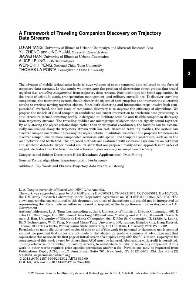
There are two kinds of operations to maintain buddies on the data stream, namely,split and merge, as shown in the following example.

Example 5. Figure 8 shows the traveling buddies in two snapshots. Traveling buddyb1 is split into three parts in snapshot s2. At the same time, b2, b3, and a part of b1 aremerged as a new buddy in s2.

When the data of a new snapshot st+1 arrives, the maintenance algorithm first up-dates the center of each buddy b. For object oi ∈ b, the system calculates the shift (�xi,�yi) between st+1 and st. And the new center is updated as

cent+1(b) = cent(b) +∑

oi∈b

(�xi,�yi).

Then every object oi ∈ b checks its distance to the buddy center; if the distanceis larger than δγ , oi will be split out as a new buddy. The cen(b) is also updated bysubtracting the shift of oi.

The second operation is to merge the buddies that are close to each other. Iftwo buddies bi and bj satisfy the following equation, they should be merged as a



Fig. 8. Example: merge and split buddies.

Fig. 9. Algorithm: buddy maintenance.

new buddy.

dist(cen(bi), cen(bj)) + γi + γ j � 2δγ

Suppose bi has mi objects and bj has mj objects, the new buddy bk’s center is computedas cen(bk) = (mi ∗ cen(bi) + mj ∗ cen(bj))/(mi + mj). Therefore, the system does not needto access the detailed coordinates of each object to merge buddies; the computation canbe done with the information from the old buddy’s center and size.

The detailed steps of buddy maintenance are shown in Figure 9. When the data ofa new snapshot arrives, the algorithm first updates the center of each buddy (line 2).Then each buddy member is checked to see whether a split operation is needed (lines3–7). At last, the system scans the buddy set and merges the buddies that are close toeach other (lines 10–13).

PROPOSITION 2. Let mbe the average number of traveling buddies and nbe the numberof objects. The time cost of Algorithm 3 is O(n + m2).



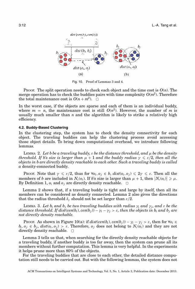
Fig. 10. Proof of Lemmas 3 and 4.

PROOF. The split operation needs to check each object and the time cost is O(n). Themerge operation has to check the buddies pairs with time complexity O(m2). Thereforethe total maintenance cost is O(n + m2).

In the worst case, if the objects are sparse and each of them is an individual buddy,where m = n, the maintenance cost is still O(n2). However, the number of m isusually much smaller than n and the algorithm is likely to strike a relatively highefficiency.

4.2. Buddy-Based Clustering

In the clustering step, the system has to check the density connectivity for eachobject. The traveling buddies can help the clustering process avoid accessingthose object details. To bring down computational overhead, we introduce followinglemmas.

LEMMA 2. Let b be a traveling buddy, ε be the distance threshold, and μ be the densitythreshold. If b’s size is larger than μ + 1 and the buddy radius γ � ε/2, then all theobjects in b are directly density reachable to each other. Such a traveling buddy is calleda density-connected buddy.

PROOF. Note that γ � ε/2, thus for ∀oi, o j ∈ b, dist(oi, o j) � 2γ � ε. Then all themembers of b are included in Nε(oi). If b’s size is larger than μ + 1, then

∣∣Nε(oi)∣∣ � μ.

By Definition 1, oi and o j are directly density reachable.

Lemma 2 shows that, if a traveling buddy is tight and large by itself, then all itsmembers can be considered as density connected. Lemma 2 also gives the directionsthat the radius threshold δγ should not be set larger than ε/2.

LEMMA 3. Let bi and bj be two traveling buddies with radius γi and γ j , and ε be thedistance threshold. If dist(cen(bi), cen(bj)) − γi − γ j > ε, then the objects in bi and bj arenot directly density reachable.

PROOF. As shown in Figure 10(a): if dist(cen(bi), cen(bj)) − γi − γ j > ε, then for ∀oi ∈bi, o j ∈ bj , dist(oi, o j) > ε. Therefore, o j does not belong to Nε(oi) and they are notdirectly density reachable.

Lemma 3 tells us that, when searching for the directly density reachable objects fora traveling buddy, if another buddy is too far away, then the system can prune all itsmembers without further computation. This lemma is very helpful. In the experimentsit helps prune more than 80% of the objects.

For the traveling buddies that are close to each other, the detailed distance compu-tation still needs to be carried out. But with the following lemmas, the system does not



Fig. 11. Algorithm: buddy-based clustering.

need to compute distances between all the pairs. Lemma 4 provides heuristics to speedup the computation.

LEMMA 4. Let bi, bj be two density-connected buddies and ε be the distance threshold.If ∃oi ∈ bi, o j ∈ bj such that dist(oi, o j) � ε, then all the objects of bi and bj are densityconnected.

PROOF. As Figure 10(b) shows, since bi is a density-connected traveling buddy and|Nε(oi)| � μ, if dist(oi, o j) � ε, then oi and o j are directly density reachable. Sinceall the objects in bi and bj are directly density reachable from oi and o j , respectively,therefore, all the objects in the two traveling buddies are density connected.

Based on Lemma 4, once the system finds a pair of objects close to each other, itends the computation and considers the corresponding buddies density connected. Thedetailed algorithm is listed in Figure 11. The algorithm first updates the buddy set in anew snapshot (line 1). Then it randomly picks a buddy and initializes it as a new cluster(lines 2–4). For each buddy in the cluster, the algorithm checks its density connectivityto others (lines 5–18). The far-away buddies are filtered out (Lines 8–9). With the helpof Lemma 4, the algorithm searches density reachable buddies and objects and addsthem to the cluster (lines 10–18). Finally, the algorithm outputs clustering results whenall the buddies are processed (line 20).

In the worst case, Algorithm 4 is still with O(n2) time complexity, where n is thenumber of objects. But in most cases, Lemmas 3 and 4 can prune the majority ofbuddies and save time for distance computation. The experiment results show thatbuddy-based clustering is an order of magnitude faster than the original clusteringalgorithm.



Fig. 12. Algorithm: buddy-based companion discovery.

4.3. Companion Discovery with Buddies

The buddies are not only useful in the clustering step, they are also helpful for theintersection process to generate companions. When intersecting a candidate with acluster, the system needs to check whether each candidate’s objects appear in the clusteror not. The information of traveling buddies can provide a shortcut to this process: If abuddy stays unchanged during the period, and it appears both in the candidate and thecluster, then the system can put all its members into the intersection result withoutaccessing the detailed objects.

To efficiently utilize the buddy information, a buddy index is designed to keep thecandidates dynamically updated with the buddies.

Definition 7 (Buddy Index). The buddy index is a triple {BID, ObjSet, CanIDs},where BID is the buddy’s ID, ObjSet is comprised of the object members of the buddy,and CanIDs records the IDs of candidates containing the buddy.

As long as the buddy stays unchanged, the candidates only store the BID instead ofdetailed objects. While making intersections, the buddy is treated as a single object.When the buddy changes, the system updates all the candidates in CanIDs and replacesBID with the corresponding objects in ObjSet. The buddy-based companion discoveryalgorithm is listed in Figure 12.

When a new snapshot arrives, the algorithm performs buddy-based clustering andupdates the buddy index (lines 2–4), then selects out the candidates with enough size(lines 5–6). The candidates are intersected with the generated clusters with the help ofthe buddy index (lines 7–10). The candidate’s duration and size are checked again afterthe intersection, and the qualified ones are output as the companions (lines 11–14).Finally, the closed candidates are added to the memory for further processing (lines15–17).

Example 6. Figure 13 shows the running process for buddy-based companion dis-covery. There are four buddies initialized in snapshot s1. In the candidates, the buddy



Fig. 13. Example: buddy-based discovery.

ID is stored instead of detailed objects. In snapshot s2, the four buddies stay the sameand the algorithm makes intersections by only checking their BIDs. Although the totalintersection time is not reduced, the time cost for each intersection operation has beenbrought down. It is common that different candidates contain the same objects, such asr1 and r3 in s2. The buddy index helps to keep only one copy of the objects and add onlypointers (the BIDs) to candidates. Therefore, the space cost is further reduced. In s3,the buddy b3 is no longer valid, then the system updates candidate r2, using the objectsto replace the buddy’s ID. In s4, traveling companion r1 is discovered as {b1, b2}. Withthe help of the buddy index, the system can easily look up detailed objects and outputthe companion as {o1, o2, o3, o4}.

5. ROAD COMPANION DISCOVERY

In the previous sections, we have investigated the problem of companion discovery on2D Euclidean space. However, many objects move on road networks in real applications.There are several unique difficulties for companion discovery on the road network. Inthis section we explore the problem of discovering road companions.

5.1. Problem Formulation

Example 7. Figure 14 shows the example of moving vehicles on the road network.There are several issues different from the companion discovery in 2D Euclidean space.



Fig. 14. Example: traveling companions on road network.

—Distance computation. In the road network, the distance between two objects shouldbe the length of the shortest path connecting them, rather than a straight linebetween them. As shown in the figure, o1 and o2 are close to each other in theEuclidean space, but they are on different directions. The road network distancebetween them is actually much larger.

—Moving direction. In most cases, the road companion moves in the shape of a line. Themoving direction of the object is an important factor in determining the companion.For example, o7, o8, and o9 in Figure 14 have neighboring vehicles o10 and o11 movingin opposite direction. Such vehicles should not be counted as the companion mem-bers. Therefore, traditional density-based clustering should be modified to model thevehicle’s moving directions.

Since the road companion discovery is a new type of problem, it is necessary tomodify some basic concepts of the traveling companion and redefine the task with newconstraints.

Definition 8 (Direct Road Connection). Let O be the object set in a snapshot, M bethe road network, and ε be the distance threshold. Object o j is directly road connectedfrom object oi on M if netd(oi, o j) ≤ ε, where netd(oi, o j) is the road network distancebetween oi and o j on M.

Note that we remove the requirements about density and replace the Euclideandistance with the road network distance in Definition 8.

Definition 9 (Road Connection). Let O be the object set in a snapshot, M be theroad network, object oi is road connected to object o j on M, if there is a chain of objects{o1, . . . , on} ∈ O where o1 = o j , on = oi such that oi+1 is directly road connected from oion M.

Based on the previous definitions, we can formally define the task of road companiondiscovery as follows.

Definition 10 (Road Companion). Let M be the road network, δs be the size thresh-old, and δt be the duration threshold, a group of objects q is called road companionif:

(1) the members of q are road connected on M for a period t where t ≥ δt;(2) q’s size size(q) ≥ δs.

Problem Definition. Let trajectory data stream S be denoted by a sequence of snapshots{s1, s2, . . . , si, . . .}. Each snapshot si = {(o1, x1,i, y1,i), (o2, x2,i, y2,i), . . . , (on, xn,i, yn,i)},



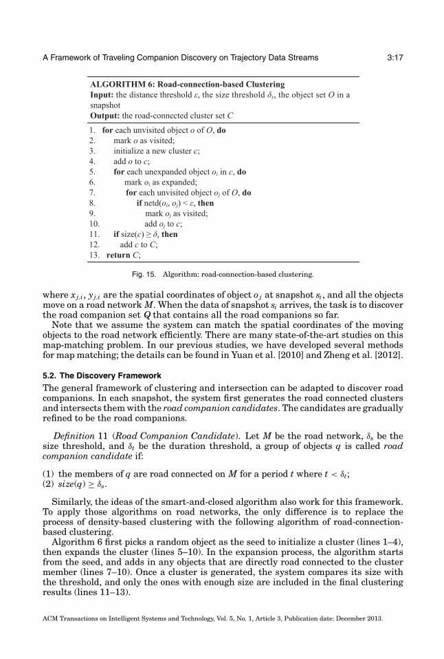
Fig. 15. Algorithm: road-connection-based clustering.

where xj,i, yj,i are the spatial coordinates of object o j at snapshot si, and all the objectsmove on a road network M. When the data of snapshot si arrives, the task is to discoverthe road companion set Q that contains all the road companions so far.

Note that we assume the system can match the spatial coordinates of the movingobjects to the road network efficiently. There are many state-of-the-art studies on thismap-matching problem. In our previous studies, we have developed several methodsfor map matching; the details can be found in Yuan et al. [2010] and Zheng et al. [2012].

5.2. The Discovery Framework

The general framework of clustering and intersection can be adapted to discover roadcompanions. In each snapshot, the system first generates the road connected clustersand intersects them with the road companion candidates. The candidates are graduallyrefined to be the road companions.

Definition 11 (Road Companion Candidate). Let M be the road network, δs be thesize threshold, and δt be the duration threshold, a group of objects q is called roadcompanion candidate if:

(1) the members of q are road connected on M for a period t where t < δt;(2) size(q) ≥ δs.

Similarly, the ideas of the smart-and-closed algorithm also work for this framework.To apply those algorithms on road networks, the only difference is to replace theprocess of density-based clustering with the following algorithm of road-connection-based clustering.

Algorithm 6 first picks a random object as the seed to initialize a cluster (lines 1–4),then expands the cluster (lines 5–10). In the expansion process, the algorithm startsfrom the seed, and adds in any objects that are directly road connected to the clustermember (lines 7–10). Once a cluster is generated, the system compares its size withthe threshold, and only the ones with enough size are included in the final clusteringresults (lines 11–13).



PROPOSITION 3. Let n be the size of object set O and N be the total node number ofroad network M. The time complexity of Algorithm 6 is O(n2 ∗ N).

PROOF. There are three loops in Algorithm 6 (lines 1, 5, and 7). In the worst case,no objects are road connected. Hence the algorithm has to run n times for the loopsin lines 1 and 7, and 1 time for the loop in line 5 (each cluster only contains oneobject in such a case). The total running number is O(n2). In each run, the systemhas to find the shortest path between objects oi and o j to compute their road networkdistance. The time cost of the shortest path searching step is determined to the detailedalgorithm and heuristics [Pearl 1984]. In the worst case, the algorithm has to visit allthe nodes of M to find out the shortest path, hence the time complexity of Algorithm 6is O(n2 ∗ N).

In many applications, the road network M contains millions of nodes, that is, Nis a quite large number. To make things worse, the system may not have enoughmemory to load in M in one time. Therefore the shortest path computation involveshuge I/O overhead. The time cost of Algorithm 6 is much larger than the density-basedclustering, and it is not feasible for efficient road companion discovery on trajectorystreams.

The bottleneck in Algorithm 6 is searching for the directly road connected objects(lines 7–10). For a particular object oi, the system has to find the shortest paths betweenoi and all unvisited objects. This computation process is the most costly step of thealgorithm. However, it is actually not necessary to compute all those shortest paths,and the algorithm’s time cost can be reduced significantly with the following lemma.

LEMMA 5. In the road network M, if the Euclidean distance between two objects oiand o j is larger than the distance threshold ε, oi and o j are not directly road connected.

PROOF. In the Euclidean space, the shortest path between oi and o j is a straight lineconnection. Since the road network M is also in the same Euclidean space, the Eu-clidean distance must be less than or equal to the road network distance: dist(oi, o j) ≤netd(oi, o j). If dist(oi, o j) > ε, then netd(oi, o j) > ε. According to Definition 8, oi and o jare not directly road connected.

Lemma 5 can help accelerate the road connection clustering process. We developa new clustering algorithm with the filtering-and-refinement strategy, as listed inFigure 16.

The main step of Algorithm 7 is at line 8. Since the main workload of the road-connection-based clustering is on the shortest path computation, Algorithm 7 is de-signed to reduce such computation and avoid the huge I/O cost of accessing the roadnetwork data. When searching for the directly road connected objects for object oi, thesystem first computes the Euclidean distance dist(oi, o j), the measure whose compu-tation only needs the coordinates of oi and o j and involves no I/O cost. If dist(oi, o j)is already larger than the threshold ε, according to Lemma 5, o j is not possible to beroad connected with o j , and the system can filter it without any further computation.In such way, about 80% of the objects are pruned and the algorithm is nearly an orderof magnitude faster in our experiments.

PROPOSITION 4. Let n be the size of object set O, N be the total node number of roadnetwork M, and m be the number of objects that pass the filtering process. The timecomplexity of Algorithm 7 is O(n2 + mN).

PROOF. With the filtering-and-refinement strategy, the algorithm only needs to com-pute road network distances for the mobjects which pass the filtering process. Thereforethe total time complexity is O(n2 + mN).



Fig. 16. Algorithm: clustering with filtering-and-refinement.

Note that m is much smaller than n with a reasonable distance threshold ε. Andthe Euclidean distance computation does not need to access the road network M. Thecomputation time and I/O overhead are reduced dramatically.

5.3. The Road-Buddy-Based Approach

The road-connection-based clustering algorithm also has the problem of individual sen-sitivity. The similar idea of traveling buddy can be applied to improve the algorithm’sefficiency. The road buddy is thus proposed to maintain small groups of objects movingtogether along the roads.

Definition 12 (Road Buddy). Let M be the road network, O be the object set, and δγ

be the buddy radius threshold, the road buddy b is defined as a set of objects satisfying:(1) b ⊆ O; (2) for ∀oi ∈ b, netd(oi, netcen(b)) ≤ δγ , where netcen(b) is the projection ofthe geometry center of b on the road network M. The buddy’s radius γ is defined as theroad network distance from netcen(b) to b’s farthest member.

To obtain netcen(b), the system needs to first compute the geometry center of b, thenemploy a map-matching algorithm to project the geometry center to the nearest road.In this study, we use the map matching algorithm developed in our previous works[Yuan et al. 2010].

The road buddy has the same operations of split and merge as the traveling buddy.Their initializations are also similar. Their major difference is at the maintenanceprocess. Because it is costly to compute the road network distance from netcen(b) to eachmember, the maintenance algorithm employs the filtering-and-refinement strategy toreduce time cost, as listed in Figure 17.

When the data of a new snapshot arrives, Algorithm 8 first computes the networkcenter of each buddy (lines 2–3), then checks each road buddy to see whether a splitoperation is needed (lines 4–11), finally scans the buddy set and merges the ones thatare close to each other (lines 12–17). The key steps of filtering-and-refinement are atlines 5, 6, 14, and 15. Before computing the road network distance between two points,



Fig. 17. Algorithm: road buddy maintenance.

the algorithm checks whether their Euclidean distance is passing the threshold andonly carries out further computation on the qualified pairs.

The road buddy can be used to improve the efficiency of road-connection-based clus-tering and companion generation by avoiding accessing the object details. Similar tothe traveling buddy, we propose several lemmas that are helpful for road companiondiscovery.

LEMMA 6. Let b be a road buddy, ε be the distance threshold. If the buddy radiusγ ≤ ε/2, then all the objects in b are directly road connected to each other. Such a roadbuddy is called a road connected buddy.

PROOF. Note that γ ≤ ε/2, thus for ∀oi, o j ∈ b, netd(oi, netcen(b)) ≤ γ andnetd(o j, netcen(b)) ≤ γ . Hence there exists a path ζ bypassing netcen(b) that connectsoi and o j , and length(ζ ) ≤ 2γ ≤ ε. Therefore netd(oi, o j) ≤ length(ζ ) ≤ ε. According toDefinition 8, oi and o j are directly road connected.

LEMMA 7. Let bi, bj be two road connected buddies and ε be the distance threshold.If ∃oi ∈ bi, o j ∈ bj such that netd(oi, o j) ≤ ε, then all the objects of bi and bj are networkconnected.

PROOF. If netd(oi, o j) ≤ ε, then oi and o j are directly road connected. Since all theobjects in bi and bj are directly road connected from oi and o j , respectively, therefore,all the objects in the two traveling buddies are road connected.

Lemma 6 and 7 can be used to speed up the road-connection-based clustering. Thelemmas show that if two buddies are tight by themselves and close to each other, thesystem can consider all their members as road connected without further computation.



Fig. 18. Algorithm: road-buddy-based clustering.

LEMMA 8. Let bi and bj be two road buddies with radius γi and γ j , and ε be thedistance threshold. If dist(netcen(bi), netcen(bj)) ≥ γi + γ j + ε, then the objects in bi andbj are not directly road connected.

PROOF. As Lemma 5 shows, the Euclidean distance is the lower bound of road net-work distance, netd(netcen(bi), netcen(bj)) ≥ dist(netcen(bi), netcen(bj)) ≥ γi +γ j +ε, thenfor ∀oi ∈ bi, o j ∈ bj , netdist(oi, o j) ≥ ε. Therefore, oi and o j are not directly networkconnected.

Lemma 8 is helpful to prune most of the unconnected buddies in road-connection-based clustering. Especially the lemma does not require the system to compute anyroad network distance on M. The system only needs the network center of buddies andtheir radius as input (which are already computed), and the huge I/O cost could besaved.

The detailed algorithm is listed in Figure 18. Algorithm 9 first calls Algorithm 8 toupdate the road buddies with new data (line 1), then randomly picks a road buddyas the seed to form a cluster (lines 2–4). The algorithm searches for the buddies thatare road connected and adds them to the cluster (lines 2–18). The buddies that aredistant from the seed are filtered out directly without detailed distance computation(lines 8–9). The algorithm searches road connected buddies with Lemmas 6 and 7 (lines10–18). Finally, the algorithm outputs the clustering results when all road buddies areprocessed (line 20).

The buddy index can be retrieved from road buddies and help companion genera-tion. Because this technique is actually independent from the metrics and distancecomputation, Algorithm 5 can be applied directly on road buddies.



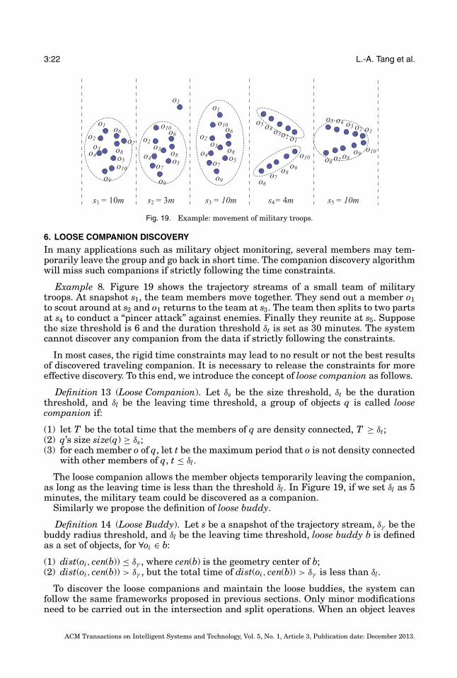
Fig. 19. Example: movement of military troops.

6. LOOSE COMPANION DISCOVERY

In many applications such as military object monitoring, several members may tem-porarily leave the group and go back in short time. The companion discovery algorithmwill miss such companions if strictly following the time constraints.

Example 8. Figure 19 shows the trajectory streams of a small team of militarytroops. At snapshot s1, the team members move together. They send out a member o1to scout around at s2 and o1 returns to the team at s3. The team then splits to two partsat s4 to conduct a “pincer attack” against enemies. Finally they reunite at s5. Supposethe size threshold is 6 and the duration threshold δt is set as 30 minutes. The systemcannot discover any companion from the data if strictly following the constraints.

In most cases, the rigid time constraints may lead to no result or not the best resultsof discovered traveling companion. It is necessary to release the constraints for moreeffective discovery. To this end, we introduce the concept of loose companion as follows.

Definition 13 (Loose Companion). Let δs be the size threshold, δt be the durationthreshold, and δl be the leaving time threshold, a group of objects q is called loosecompanion if:

(1) let T be the total time that the members of q are density connected, T ≥ δt;(2) q’s size size(q) ≥ δs;(3) for each member o of q, let t be the maximum period that o is not density connected

with other members of q, t ≤ δl.

The loose companion allows the member objects temporarily leaving the companion,as long as the leaving time is less than the threshold δl. In Figure 19, if we set δl as 5minutes, the military team could be discovered as a companion.

Similarly we propose the definition of loose buddy.

Definition 14 (Loose Buddy). Let s be a snapshot of the trajectory stream, δγ be thebuddy radius threshold, and δl be the leaving time threshold, loose buddy b is definedas a set of objects, for ∀oi ∈ b:

(1) dist(oi, cen(b)) ≤ δγ , where cen(b) is the geometry center of b;(2) dist(oi, cen(b)) > δγ , but the total time of dist(oi, cen(b)) > δγ is less than δl.

To discover the loose companions and maintain the loose buddies, the system canfollow the same frameworks proposed in previous sections. Only minor modificationsneed to be carried out in the intersection and split operations. When an object leaves



Fig. 20. Experiment settings.

the companion candidate or buddy, the system does not remove that object or split thebuddy immediately, instead puts the object/buddy in a buffer to be removed/split after atime period of δl. If the object returns in δl, the remove/split command will be canceled.Such modification does not influence the general frameworks of companion discovery.The other steps of the clustering-and-intersection algorithm, smart-and-closed method,and the buddy-based approach remain the same for loose companion discovery, hencewe omit the details here due to space limitation.

7. PERFORMANCE EVALUATION

7.1. Experiment Setup

Datasets. We evaluate the proposed methods on both real and synthetic trajectorydatasets. The taxi dataset (D1) is retrieved from the Microsoft GeoLife and T-Driveprojects [Yuan et al. 2010; Zheng et al. 2010] with the road network of Beijing. Thetrajectories are generated from GPS devices installed on 500 taxis in the city of Beijing.The dataset is available to the public5. The military trajectory dataset (D2) is retrievedfrom the CBMANET project [Krout 2007], in which an infantry battalion of 780 units,divided as 30 teams, moves from Fort Dix to Lakehurst for a mission on two routesin 3 hours. Meanwhile, to test the algorithm’s performance in large datasets, we alsogenerate two synthetic datasets (D3 and D4), being comprised of 1,000 to 10,000 objects,with more than 10 million data records.

Baselines. The proposed Smart-and-Closed algorithm (SC) and Buddy-based discov-ery algorithm (BU) are compared with Clustering-and-Intersection method (CI), whichis used as the framework to find convoy patterns [Jeung et al. 2008]; and two state-of-the-art algorithms: (1) The Swarm pattern (SW) [Li et al. 2010] that captures theobjects moving within arbitrary shape of clusters for certain snapshots that are possi-bly nonconsecutive; (2) the TraClu algorithm (TC) [Lee et al. 2007] that discovers thecommon subtrajectories with a density-based line-segment clustering algorithm.

Environments. The experiments are conducted on a PC with Intel 6400 Dual CPU2.13 GHz and 2.00GB RAM. The operating system is Windows 7 Enterprise. All thealgorithms are implemented in Java on the Eclipse 3.3.1 platform with JDK 1.6.0. Theparameter settings are listed in Figure 20.

7.2. Comparisons in Discovery Efficiency

In this section we conduct experiments to evaluate the efficiency of companion discov-ery algorithms in Euclidean space. Since both SW and TC cannot output the resultsincrementally, we take the running time of the entire dataset as the measure for time

5GeoLife GPS Trajectories Datasets. Released at: http://research.microsoft.com/en-us/downloads/b16d359d-d164-469e-9fd4-daa38f2b2e13/default.aspx.



Fig. 21. Efficiency: (a) time, (b) space on different datasets.

Fig. 22. Efficiency: (a) time, (b) space versus δs.

cost. The size of candidate set (number of objects) is used to measure the space cost ofcompanion computation. The only exception is TC, where since the algorithm only car-ries out the subtrajectory clustering task and does not store any companion candidates,TC’s space cost is not included in the experiment.

We first evaluate the algorithm’s time and space costs on different datasets withdefault settings. Figure 21 shows the experiment results. Note that the y-axes are inlogarithmic scale. BU achieves the best performances on all the datasets. In the largestdataset D4, BU is an order of magnitude faster than CI and SW. BU’s space cost is only20% of SW and less than 5% of CI.

Figure 22 illustrates the influences of companion size threshold δs in the experi-ments. The experiment is carried on dataset D3. Based on default settings, we evaluatethe algorithms with different values of δs. Generally speaking, when the size thresholdgrows larger, the filtering mechanism is more effective to prune more companion can-didates in each snapshot. The space costs reduce significantly, and the running timesalso decrease for fewer intersections.

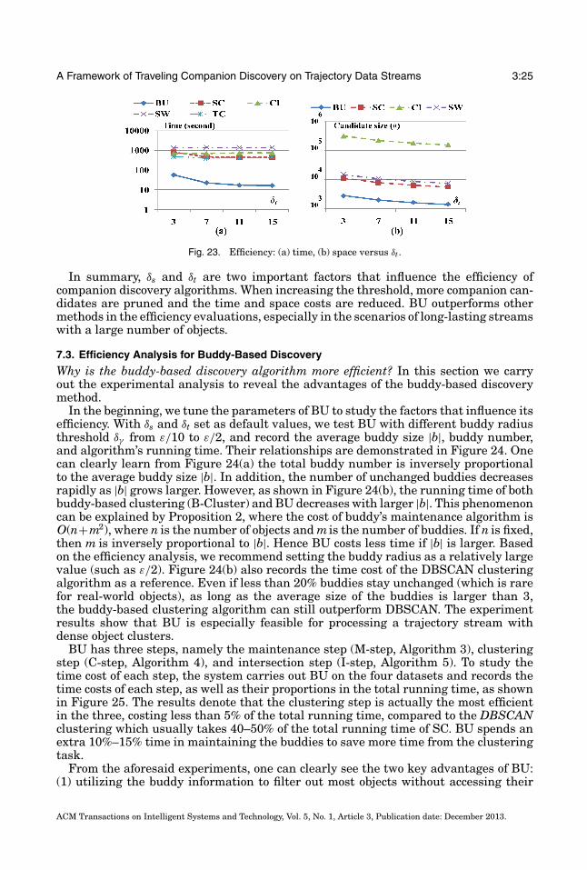
We also study the influence of duration threshold δt. Based on default settings, theexperiments are conducted on dataset D3. The value of δt is changed from 3 to 15, andthe algorithm’s performances are shown in Figure 23. BU, SC, and CI are all fasterwhen δt grows larger, because many companion candidates are not consistent enoughto last for a long time. When setting δt as 15 snapshots, BU can process the datasetin less than 20 seconds (Figure 23(a)). It is almost an order of magnitude faster thanSC and CI. TC is not influenced by δs and δt, since it is only a clustering algorithm anddoes not generate any companion candidates. Beside TC, SW also could not improvethe performance when δt increases. The reason is SW utilizes the object growth strategyto prune candidates. Such heuristics could only work with the size threshold δs, butcannot benefit from larger δt.



Fig. 23. Efficiency: (a) time, (b) space versus δt.

In summary, δs and δt are two important factors that influence the efficiency ofcompanion discovery algorithms. When increasing the threshold, more companion can-didates are pruned and the time and space costs are reduced. BU outperforms othermethods in the efficiency evaluations, especially in the scenarios of long-lasting streamswith a large number of objects.

7.3. Efficiency Analysis for Buddy-Based Discovery

Why is the buddy-based discovery algorithm more efficient? In this section we carryout the experimental analysis to reveal the advantages of the buddy-based discoverymethod.

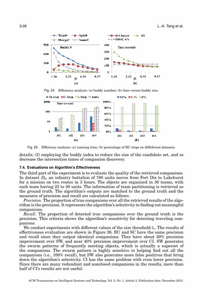
In the beginning, we tune the parameters of BU to study the factors that influence itsefficiency. With δs and δt set as default values, we test BU with different buddy radiusthreshold δγ from ε/10 to ε/2, and record the average buddy size |b|, buddy number,and algorithm’s running time. Their relationships are demonstrated in Figure 24. Onecan clearly learn from Figure 24(a) the total buddy number is inversely proportionalto the average buddy size |b|. In addition, the number of unchanged buddies decreasesrapidly as |b| grows larger. However, as shown in Figure 24(b), the running time of bothbuddy-based clustering (B-Cluster) and BU decreases with larger |b|. This phenomenoncan be explained by Proposition 2, where the cost of buddy’s maintenance algorithm isO(n+m2), where n is the number of objects and m is the number of buddies. If n is fixed,then m is inversely proportional to |b|. Hence BU costs less time if |b| is larger. Basedon the efficiency analysis, we recommend setting the buddy radius as a relatively largevalue (such as ε/2). Figure 24(b) also records the time cost of the DBSCAN clusteringalgorithm as a reference. Even if less than 20% buddies stay unchanged (which is rarefor real-world objects), as long as the average size of the buddies is larger than 3,the buddy-based clustering algorithm can still outperform DBSCAN. The experimentresults show that BU is especially feasible for processing a trajectory stream withdense object clusters.

BU has three steps, namely the maintenance step (M-step, Algorithm 3), clusteringstep (C-step, Algorithm 4), and intersection step (I-step, Algorithm 5). To study thetime cost of each step, the system carries out BU on the four datasets and records thetime costs of each step, as well as their proportions in the total running time, as shownin Figure 25. The results denote that the clustering step is actually the most efficientin the three, costing less than 5% of the total running time, compared to the DBSCANclustering which usually takes 40–50% of the total running time of SC. BU spends anextra 10%–15% time in maintaining the buddies to save more time from the clusteringtask.

From the aforesaid experiments, one can clearly see the two key advantages of BU:(1) utilizing the buddy information to filter out most objects without accessing their



Fig. 24. Efficiency analysis: (a) buddy number; (b) time versus buddy size.

Fig. 25. Efficiency analysis: (a) running time; (b) percentage of BU steps on diffeferent datasets.

details; (2) employing the buddy index to reduce the size of the candidate set, and sodecrease the intersection times of companion discovery.

7.4. Evaluations on Algorithm’s Effectiveness

The third part of the experiment is to evaluate the quality of the retrieved companions.In dataset D2, an infantry battalion of 780 units moves from Fort Dix to Lakehurstfor a mission on two routes in 3 hours. The objects are organized in 30 teams, witheach team having 25 to 30 units. The information of team partitioning is retrieved asthe ground truth. The algorithm’s outputs are matched to the ground truth and themeasures of precision and recall are calculated as follows.

Precision. The proportion of true companions over all the retrieved results of the algo-rithm is the precision. It represents the algorithm’s selectivity in finding out meaningfulcompanions.

Recall. The proportion of detected true companions over the ground truth is theprecision. This criteria shows the algorithm’s sensitivity for detecting traveling com-panions.

We conduct experiments with different values of the size threshold δs. The results ofeffectiveness evaluation are shown in Figure 26. BU and SC have the same precisionand recall since they output identical companions. They have about 20% precisionimprovement over SW, and near 40% precision improvement over CI. SW generatesthe swarm patterns of frequently meeting objects, which is actually a superset ofthe companions. The swarm pattern is highly sensitive to helping find out all thecompanions (i.e., 100% recall), but SW also generates more false positives that bringdown the algorithm’s selectivity. CI has the same problem with even lower precision.Since there are many redundant and nonclosed companions in the results, more thanhalf of CI’s results are not useful.



Fig. 26. Effectiveness: (a) precision, (b) recall versus δs.

Fig. 27. Effectiveness: (a) precision, (b) recall versus δt.

Again, TC is not affected by the parameters of δs and δt. TC takes the movementdirection as an important measure to compute subtrajectory clusters; its results reflectthe major directions of the object movements. However, such clusters may not capturethe information of companions, because the companion member’s moving directionmight be different. As an illustration, please go back to Figure 1. From snapshot s2 tos3, the moving directions of o8 and o9 are different, hence they may be put in differentsubtrajectory clusters.

Another interesting observation is that, in Figure 26, BU, SC, CI, and SW’s precisionsall increase when δs becomes larger, since fewer companions can pass a higher sizethreshold. However, if δs is set too high (more than 25), several true companions willalso be filtered out and the algorithm cannot achieve 100% recall.

In the next experiment, we study the influence of time threshold δt. Figure 27 showsthe precision and recall of the five algorithms with different δt on D2. BU and SC achievebetter performance than SW and CI. When increasing δt, the algorithm’s precisionincreases, but they can still keep a high recall. Since all the true companions last fora long period in D2, if we set δt greater than 11, both BU and SC can achieve 100%precision and recall. However, if δt is set too high, for example, 15, no companion canbe discovered since there exist no object groups moving together for such a long time.

In general, BU and SC can guarantee 100% recall (i.e., not missing any real com-panion), we suggest that in real applications, the user should set a relatively high timethreshold to filter out false positives, but a moderate size threshold to guarantee thealgorithm’s sensitivity.

7.5. Experiments on Road Companion Discovery

To test the efficiency of road companion discovery, we perform the evaluation on datasetD1 with the road network of Beijing, which has 106,579 road nodes and 141,380



Fig. 28. Efficiency: (a) time; (b) I/O of road companion discovery versus δs.

Fig. 29. Efficiency: (a) time; (b) I/O of road companion discovery versus δt.

road segments. The default size threshold δs is set as 8 and the time threshold δtis set as 11. In this experiment, we compare the performance of four methods: (1) theClustering-and-Intersection framework with road network distance computation (CI);(2) the Smart-and-Closed algorithm with road network distance computation (SC);(3) the smart-and-closed algorithm with Filtering-and-Refinement strategy (FR); and(4) The Road-Buddy-based method (RB).

We first evaluate the time and space costs of road companion discovery. The numberof accessed road nodes is used as the measure for I/O cost. Based on default settings, weevaluate the algorithms with different values of δs. Figure 28 shows the running timeand accessed node number. Generally speaking, when the size threshold grows larger,both running time and I/O costs decrease. The computation cost of road companiondiscovery is much larger than the traveling companion discovery on Euclidean space.This is mainly caused by the high I/O overhead in road network distance computation.Since the road network distance computation becomes the major cost, SC cannot savemuch time comparing to CI. However, FR and RB are an order of magnitude fasterthan SC and CI, because they utilize the filtering-and-refinement strategy to avoidmost unnecessary road network distance computations. The effects of RB are better,since RB groups the objects in small buddies and limits the distance computation in asmall region with lower I/O overhead.

The influence of duration threshold δt is also studied in our experiment. Based ondefault settings, the value of δt is changed from 3 to 15; the algorithms’ performancesare shown in Figure 29. All the algorithms run faster when δt grows larger, becausefewer road companion candidates can last for a long time. Again, RB and FR only cost20%–50% time as CI and SC.

The experiment results show that the main bottleneck of road companion discoveryis at the distance computation stage. The traditional companion discovery methods,



Fig. 30. Efficiency: (a) time; (b) space versus δl.

Fig. 31. Effectiveness: (a) precision; (b) recall versus δl.

BU and SC, do not work well on the road networks. The new frameworks of RB andFR reduce the time cost on unnecessary shortest path computation, therefore they canachieve higher efficiency peformances.

7.6. Evaluations on Loose Companion Discovery

In the previous experiments, we set the leaving threshold δl as 0. In this section, weconduct experiments on loose companion discovery. We run the algorithms of BU, SC,and CI on dataset D3 by tuning δl from 0–6 snapshots.

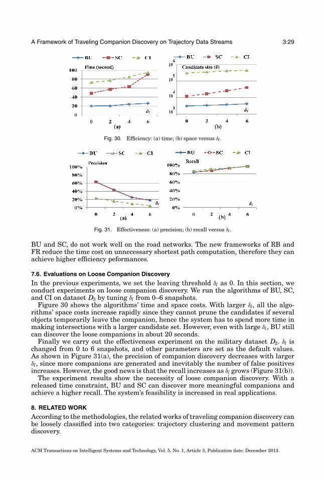
Figure 30 shows the algorithms’ time and space costs. With larger δl, all the algo-rithms’ space costs increase rapidly since they cannot prune the candidates if severalobjects temporarily leave the companion, hence the system has to spend more time inmaking intersections with a larger candidate set. However, even with large δl, BU stillcan discover the loose companions in about 20 seconds.

Finally we carry out the effectiveness experiment on the military dataset D2. δl ischanged from 0 to 6 snapshots, and other parameters are set as the default values.As shown in Figure 31(a), the precision of companion discovery decreases with largerδl, since more companions are generated and inevitably the number of false positivesincreases. However, the good news is that the recall increases as δl grows (Figure 31(b)).

The experiment results show the necessity of loose companion discovery. With areleased time constraint, BU and SC can discover more meaningful companions andachieve a higher recall. The system’s feasibility is increased in real applications.

8. RELATED WORK

According to the methodologies, the related works of traveling companion discovery canbe loosely classified into two categories: trajectory clustering and movement patterndiscovery.



8.1. Trajectory Clustering

The works in this category focus on developing efficient algorithms to cluster movingobjects. Gaffney and Smyth first proposed the fundamental principles of clusteringmoving objects based on the theories of probabilistic modeling [Gaffney and Smyth1999; Cadez et al. 2000]. Many distance functions, such as DTW [Yi et al. 1998] andLCSS [Gunopoulos 2002] are proposed. Lee et al. proposed a novel partition-and-groupframework to find the clusters based on subtrajectories [Lee et al. 2007].

In Har-Peled [2003], Har-Peled shows that the moving objects can be clustered whenthe resulting clusters are competitive at any time during the motion. Yang et al. pro-posed the idea of a neighbor-based pattern detection method for windows [Yang et al.2009]. Ester et al. made the progress to generate incremental clusters [Ester et al.1998]. Li et al. propose a microcluster [Li et al. 2004] based schema to cluster movingobjects. Zhang and Lin use the k-center clustering algorithm [Gonzalez 1985] for his-togram construction. A distance function combining velocity and position differencesis proposed in their work [Zhang and Lin 2004]. More recently, Jensen et al. utilize thevelocity features to cluster objects for the current and near future positions [Jensenet al. 2007].

However, as pointed out in Jeung et al. [2008], most of the aforsaid methods cannotbe used directly for traveling companion discovery. The major problem is that thosealgorithms tend to generate clusters for the entire trajectory dataset, instead of eachsnapshot. Hence the detailed object relationships and evolving companion patternsare all lost. In addition, some algorithms require the object’s velocity in advance andneed to scan the data for multiple times. Such requirements are not fit for trajectorystreams.

8.2. Movement Pattern Discovery

Movement pattern discovery is a hot topic in recent years. The problem has beenvariously referred to as the search for flocks [Gudmundsson and Kreveld 2006], movingclusters [Kalnis et al. 2005], spatial-tempo joins [Bakalov et al. 2005], spatial colocations[Yoo and Shekhar 2004], meetings [Gudmundsson et al. 2004], convoys [Jeung et al.2008], moving groups [Aung 2008], swarms [Li et al. 2010] and so on.

One of the earliest works is flock discovery [Gudmundsson et al. 2004]. A flock isdefined as a group of objects moving together within a circular region [Gudmundssonand Kreveld 2006]. There are several variations of this model: Variable flock permitsthe members to change during the time span [Benkert et al. 2008],while meeting isa circle similar to flock but fixed in a single location all the time [Gudmundsson andKreveld 2006]. However, such shapes are restricted to circles and the results are alsosensitive to the parameter of radius.

Li et al. designed a flow scan algorithm for hot route mining [Li et al. 2007]. Liu etal. mined frequent trajectory patterns by using RF tag arrays. Their work successfullydemonstrated the feasibility and the effectiveness of movement patterns in real life [Liuet al. 2007]. Tao et al. proposed the technique of spatio-temporal aggregation using asketch index. This method can process the queries an order of magnitude faster thanthe previous works [Tao et al. 2004]. Giannotti et al. proposed the interest-region-basedmining algorithm [Giannotti et al. 2007]. Horvitz et al. propose the models of usinggroups of mobile users to discover congestions in urban areas [Horvitz et al. 2005].The shortest path problem has been studied on land surface [Xing and Shahabi 2010;Liu and Wong 2011] and this technique has been used to process the k-NN queries[Shahabi et al. 2008; Xing et al. 2009]. Tao et al. propose the techniques to find k-skipshortest paths [Tao et al. 2011]. Yuan et al. present a cloud-based system computingcustomized and practically fast driving routes for an end-user using traffic conditionsand driver behavior, which is a milestone study in this field [Yuan et al. 2011].



Fig. 32. The comparison with related works.

Zhang et al. propose the techniques to produce intersections of streaming movingobjects [Zhang et al. 2008, 2011]. This method is a big improvement from existingalgorithms by the speedup of several orders of magnitude. Nutanong et al. use a saferegion to report objects that do not change over time [Nutanong et al. 2008, 2010].The proposed V*-Diagram has much smaller I/O and computation costs than previousmethods. It outperforms the best existing technique by two orders of magnitude.

However, since the preceding methods focus more on discovering hot spots, regions, orroutes rather than object groups, they cannot be used directly for companion discovery.

Kalnis et al. proposed the first study to automatic extraction of moving clusters fromlarge spatial datasets [Kalnis et al. 2005]. In a recent work, Jeung et al. proposed theframework of convoy query [Jeung et al. 2008]. It is a significant step forward in theworks of movement pattern mining, since it allows the objects to organize in arbitraryshapes. Li et al. further released the constraints of convoy and proposed the swarmpattern to discover object groups in a sporadic way [Li et al. 2010].

The concepts of convoy and swarm patterns are similar to traveling companion.However, the convoy mining algorithm needs to scan the entire trajectory into memoryto make trajectory simplification, and the system also needs to load the whole datasetinto memory to search for swarms. It is impractical to use such a method in a datastream environment. The swarm pattern is a frequent itemset-based concept. Since itis difficult to detect large size frequent itemsets [Zhu et al. 2007], the swarm patternhas limited applicability for datasets with large-scale objects. The major advantage ofthe companion discovery technique is about the discovery efficiency. The buddy-basedmethod can discover the companions of arbitrary shapes an order of magnitude faster.Hence it is a feasible method to be applied in the data stream scenarios of huge amountof trajectories.

Figure 32 compares the features of some related methods with the proposed algo-rithms to discovery of traveling companions, road companions, and loose companions.

9. CONCLUSION AND FUTURE WORK

In this study we investigate the problem of traveling companion discovery on trajectorydata streams. We propose the algorithms of smart-and-closed discovery to efficientlygenerate companions from trajectory data. The model of traveling buddy is proposedto help improve both the clustering and intersection processes for companion discov-ery. The proposed methods are extended to more complex scenarios for road compan-ion and loose companion discovery. We evaluate the proposed algorithms in extensive



experiments on both real and synthetic datasets. The buddy-based method is shown tobe an order of magnitude faster than existing approaches on both Euclidean space androad networks. The effectiveness of the buddy-based algorithm also outperforms othercompetitors in terms of precision and recall.

In the future, we are going to integrate the companion discovery methods toreal application services such as battlefield monitoring systems and traffic analysisservices.

REFERENCES

AUNG, H.-H. 2008. Discovering moving groups of tagged objects. Tech. rep., National University of Singapore.http://www.nus.edu.sg/.

BAKALOV, P., HADJIELEFTHERIOU, M., AND TSOTRAS, V. J. 2005. Time relaxed spatiotemporal trajectory joins.In Proceedings of the 13th Annual ACM International Workshop on Geographic Information Systems(GIS’05). 182–191.

BENKERT, M., GUDDMUNDSSON, J., HUBNER, F., AND WOLLE, T. 2008. Reporting flock patterns. Comput. Geom.Theory Appl. 41, 3, 111–125.

CADEZ, I. V., GAFFNEY, S., AND SMYTH, P. 2000. A general probabilistic framework for clustering individualsand objects. In Proceedings of the 6th ACM SIGKDD International Conference on Knowledge Discoveryand Data Mining (KDD’00). 140–149.

ESTER, M., KRIEGEL, H.-P., SANDER, J.,WIMMER, M., AND XU, X. 1998. Incremental clustering for mining in adata warehousing environment. In Proceedings of the 24th International Conference on Very Large DataBases (VLDB’98). 323–333.

ESTER, M., KRIEGEL, H.-P., SANDER, J., AND XU, X. 1996. A density-based algorithm for discovering clustersin large spatial databases with noise. In Proceedings of the 2nd International Conference on KnowledgeDiscovery and Data Mining (KDD’96). 226–231.

GAFFNEY, S. AND SMYTH, P. 1999. Trajectory clustering with mixtures of regression models. In Proceedingsof the 5th ACM SIGKDD International Conference on Knowledge Discovery and Data Mining (KDD’99).63–72

GIANNOTTI, F., NANNI, M., PEDRESCHI, D., AND PINELLI, F. 2007. Trajectory pattern mining. In Proceedings ofthe 13th ACM SIGKDD International Conference on Knowledge Discovery and Data Mining (KDD’07).330–339.

GONZALEZ, T. 1985. Clustering to minimize the maximum intercluster distance. Theor. Comput. Sci. 38,293–306.

GUDMUNDSSON, J. AND KREVELD, M. V. 2006. Computing longest duration flocks in trajectory data. In Proceed-ings of the 14th Annual ACM International Symposium on Advances in Geographic Information Systems(GIS’06). 35–42.

GUDMUNDSSON, J., KREVELD, M. V., AND SPECKMANN, B. 2004. Efficient detection of motion patterns in spatio-temporal data sets. In Proceedings of the 12th Annual ACM International Workshop on GeographicInformation Systems (GIS’04). 250–257.

GUNOPOULOS, D. 2002. Discovering similar multidimensional trajectories. In Proceedings of the 18th Interna-tional Conference on Data Engineering (ICDE’02). 673–684.

HAN, J. AND KAMBER, M. 2006. Data Mining: Concepts and Techniques 2nd Ed. Morgan Kaufmann.HAR-PELED, S. 2003. Clustering motion. Discr. Comput. Geom. 31, 4, 545–565.HORVITZ, E., APACIBLE, J., SARIN, R., AND LIAO, L. 2005. Prediction, expectation, and surprise: Methods, designs,

and study of a deployed traffic forecasting service. In Proceedings of the 21st Conference on Uncertaintyin Artificial Intelligence (UAI’05).

JENSEN, C. S., LIN, D., AND OOI, B. C. 2007. Continuous clustering of moving objects. IEEE Trans. Knowl. DataEngin. 19, 9, 1161–1174.

JEUNG, H., YIU, M. L., ZHOU, X., JENSEN, C. S., AND SHEN, H. T. 2008. Discovery of convoys in trajectory databases.Proc. VLDB Endow. 1, 1, 1068–1080.

KALNIS, P., MAMOULIS, N., AND BAKIRAS, S. 2005. On discovering moving clusters in spatial-temporal data.In Proceedings of the 9th International Conference on Advances in Spatial and Temporal Databases(SSTD’05). 364–381.

KROUT, T. 2007. Cb manet scenario data distribution. Tech. rep., BBN.LEE, J.-G., HAN, J., AND WHANG, K.-Y. 2007. Trajectory clustering: A partition-and-group framework. In Pro-

ceedings of the ACM SIGMOD International Conference on Management of Data (SIGMOD’07). 593–604.



LEE, M., HSU, W., JENSEN, C. S., CUI, B., AND TEO, K. 2003. Supporting frequent updates in r-trees: A bottom-upapproach. The VLDB J. 18, 3, 719–738.

LI, X., HAN, J., LEE, J.-G., AND GONZALEZ, H. 2007. Traffic density based discovery of hot routes in roadnetworks. In Proceedings of the 10th International Conference on Advances in Spatial and TemporalDatabases (SSTD’07). 441–459.

LI, Y., HAN, J., AND YANG, J. 2004. Clustering moving objects. In Proceedings of the 10th ACM SIGKDDInternational Conference on Knowledge Discovery and Data Mining (KDD’04). 617–622.

LI, Z., DING, B., HAN, J., AND KAYS, R. 2010. Swarm: Mining relaxed temporal moving object clusters accuratediscovery of valid convoys from moving object trajectories. Proc. VLDB Endow. 3, 723–734.

LIU, L. AND WONG, R. C.-W. 2011. Finding shortest path on land surface. In Proceedings of the ACM SIGMODInternational Conference on Management of data (SIGMOD’11). 433–444.

LIU, Y., CHEN, L., PEI, J., CHEN, Q., AND ZHAO, Y. 2007. Mining frequent trajectory patterns for activitymonitoring using radio frequency tag arrays. In Proceedings of the 5th IEEE International Conferenceon Pervasive Computing and Communications (PerCom’07).

NUTANONG, S., ZHANG, R., TANIN, E., AND KULIK, L. 2008. The v*-diagram: A query dependent approach tomoving knn queries. Proc. VLDB Endow. 1, 1, 1095–1106.

NUTANONG, S., ZHANG, R., TANIN, E., AND KULIK, L. 2010. Analysis and evaluation of v*-knn: An efficientalgorithm for moving knn queries. VLDB J. 19, 3, 307–332.

PEARL, J. 1984. Heuristics: Intelligent Search Strategies for Computer Problem Solving. Addison-WesleyLongman Publishing Co.

SHAHABI, C., TANG, L. A., AND XING, S. 2008. Indexing land surface for efficient knn query. Proc. VLDB Endow.1, 1, 1020–1031.

TANG, L.-A., YU, X., KIM, S., HAN, J., HUNG, C.-C., AND PENG, W.-C. 2010. Tru-alarm: Trustworthiness analysisof sensor networks in cyber-physical systems. In Proceedings of the IEEE International Conference onData Mining (ICDM’10). 1079–1084.

TANG, L.-A., ZHENG, Y., XIE, X., YUAN, J., YU, X., AND HAN, J. 2011. Retrieving k-nearest neighboring trajectoriesby a set of point locations. In Proceedings of the 12th International Conference on Advances in Spatialand Temporal Databases (SSTD’11). 223–241.

TANG, L.-A., ZHENG, Y., YUAN, J., HAN, J., LEUNG, A., HUNG, C.-C., AND PENG, W.-C. 2012. On discovery of travelingcompanions from streaming trajectories. In Proceedings of the 28th IEEE International Conference onData Engineering (ICDE’12). 186–197.

TAO, Y., KOLLIOS, G., CONSIDINE, J., LI, F., AND PAPADIAS, D. 2004. Spatio-temporal aggregation using sketches.In Proceedings of the 20th IEEE International Conference on Data Engineering (ICDE’04). 214.

TAO, Y., SHENG, C., AND PEI, J. 2011. On k-skip shortest paths. In Proceedings of the ACM SIGMOD Interna-tional Conference on Management of Data (SIGMOD’11). 421–432.

XING, S. AND SHAHABI, C. 2010. Scalable shortest paths browsing on land surface. In Proceedings of the 18th

SIGSPATIAL International Conference on Advances in Geographic Information Systems (GIS’10). 89–98.XING, S., SHAHABI, C., AND PAN, B. 2009. Continuous monitoring of nearest neighbors on land surface. Proc.

VLDB Endow. 2, 1, 1114–1125.YANG, D., RUNDENSTEINER, E. A., AND WARD, M. O. 2009. Neighbor-based pattern detection for windows over

streaming data. In Proceedings of the 12th International Conference on Extending Database Technology:Advances in Database Technology (EDBT’09). 529–540.

YI, B., JAGADISH, H. V., AND FALOUTSOS, C. 1998. Efficient retrieval of similar time sequences under timewarping. In Proceedings of the 14th International Conference on Data Engineering (ICDE’98). 201–208.

YOO, J. S. AND SHEKHAR, S. 2004. A partial join approach for mining co-location patterns. In Proceedings of the12th Annual ACM International Workshop on Geographic Information Systems (GIS’04). 241–249.

YUAN, J., ZHENG, Y., XIE, X., AND SUN, G. 2011. Driving with knowledge from the physical world. In Proceedingsof the 17th ACM SIGKDD International Conference on Knowledge Discovery and Data Mining (KDD’11).316–324.

YUAN, J., ZHENG, Y., ZHANG, C., XIE, W., XIE, X., SUN, G., AND HUANG, Y. 2010. T-drive: Driving directions basedon taxi trajectories. In Proceedings of the 18th SIGSPATIAL International Conference on Advances onGeographical Information Systems (GIS’10). 99–108.

ZHANG, Q. AND LIN, X. 2004. Clustering moving objects for spatial-temporal selectivity estimation. In Proceed-ings of the 15th Australasian Database Conference (ADC’04). 123–130.

ZHANG, R., LIN, D., RAMAMOHANARAO, K., AND BERTINO, E. 2008. Continuous intersection joins over movingobjects. In Proceedings of the 24th International Conference on Data Engineering (ICDE’08). 863–872.

ZHANG, R., QI, J., LIN, D., WANG, W., AND WONG, R. C.-W. 2011. A highly optimized algorithm for continuousintersection join queries over moving objects. VLDB J. 21, 4, 561–586.



ZHENG, K., ZHENG, Y., XIE, X., AND ZHOU, X. 2012. Reducing uncertainty of low-sampling-rate trajectories. InProceedings of the 28th IEEE International Conference on Data Engineering (ICDE’12). 1144–1155.

ZHENG, Y., XIE, X., AND MA, W. 2010. GeoLife: A collaborative social networking service among user, locationand trajectory. IEEE Data Engin. Bull. 33, 2, 32–40.

ZHENG, Y. AND ZHOU, X. 2011. Computing with Spatial Trajectories. Springer.ZHU, F., YAN, X., HAN, J., YU, P. S., AND CHENG, H. 2007. Mining colossal frequent patterns by core pattern

fusion. In Proceedings of the 23rd International Conference on Data Engineering (ICDE’07). 706–715.

Received February 2012; revised March 2012; accepted May 2012


Documents

A framework of traveling companion discovery on trajectory data streams