'$ ��

' $ � ��

I N F O R M A T I K

� �

A Framework of

Refutational Theorem Proving

for

Saturation-BasedDecision Procedures

Yevgeny Kazakov

MPI–I–2005–2-004 August 2005

FORSCHUNGSBERICHT RESEARCH REPORT

M A X - P L A N C K - I N S T I T U TFÜR

I N F O R M A T I K

Stuhlsatzenhausweg 85 66123 Saarbrücken Germany

Authors’ Addresses

Max-Planck-Institut für InformatikStuhlsatzenhausweg 8566123 SaarbrückenGermanyPhone: +49 681 9325-215Fax: +49 681 9325-299Email: ykazakov@mpi-inf.mpg.de

Acknowledgements

The author has been supported by the International Max Planck ResearchSchool for computer science (IMPRS). I would like to thank Hans de Nivellefor reading several sections of this report and providing a valuable feedback.

Abstract

Automated state-of-the-art theorem provers are typically optimised for par-ticular strategies, and there are only limited number of options that can beset by the user. Probably because of this, the general conditions on ap-plicability of saturation-based calculi have not been thoroughly investigated.However for some applications, e.g., for saturation-based decision procedures,one would like to have more options in order to design flexible saturationstrategies.

In this report we revisit several well-known saturation-based calculi usedin automated deduction: Ordered Resolution, Ordered Paramodulation, Su-perposition and Chaining calculi. We give a uniform account on completenessproofs for these calculi using the standard model construction procedures ofBachmair and Ganzinger. By careful inspection of these proofs, we formulatesome variations of inference rules and general conditions on orderings underwhich the calculi remain refutationally complete. In particular, we consid-erably generalise the known class of admissible orderings for the Chainingcalculi.

We also consider in details the standard notion of redundancy, estimatethe complexity for the steps of the clause normal form transformation, andgive a computational model of the saturation process.

Keywords

Automated deduction, Theorem proving

Contents

Contents 1

1 Introduction 3

2 Logical Preliminaries 52.1 First-Order Logic . . . . . . . . . . . . . . . . . . . . . . . . . . . . 5

2.1.1 Syntax of first-order logic . . . . . . . . . . . . . . . . . . . 52.1.2 Semantics of first-order logic . . . . . . . . . . . . . . . . . . 8

2.2 First-Order Clause Logic . . . . . . . . . . . . . . . . . . . . . . . . 102.3 Term Rewrite Systems . . . . . . . . . . . . . . . . . . . . . . . . . 152.4 Orderings . . . . . . . . . . . . . . . . . . . . . . . . . . . . . . . . 19

2.4.1 Multiset and lexicographic extensions of orderings . . . . . . 192.4.2 Reduction orders . . . . . . . . . . . . . . . . . . . . . . . . 212.4.3 The ordered Knuth-Bendix completion . . . . . . . . . . . . 24

2.5 Substitutions And Unification . . . . . . . . . . . . . . . . . . . . . 252.6 Covering Expressions and Atomic Substitutions . . . . . . . . . . . 282.7 Saturation-Based Theorem Proving . . . . . . . . . . . . . . . . . . 32

3 The Ordered Resolution Calculus 353.1 Refutational Completeness for the Ground Version . . . . . . . . . . 363.2 Refinements of the Resolution Calculus . . . . . . . . . . . . . . . . 403.3 Redundancy: the Static View . . . . . . . . . . . . . . . . . . . . . 443.4 Redundancy: the Dynamic View . . . . . . . . . . . . . . . . . . . . 453.5 Lifting . . . . . . . . . . . . . . . . . . . . . . . . . . . . . . . . . . 513.6 Selection Functions for General Clauses . . . . . . . . . . . . . . . . 563.7 Hyper-Resolution Strategies . . . . . . . . . . . . . . . . . . . . . . 58

4 Equational Reasoning 594.1 The Ordered Paramodulation Calculus . . . . . . . . . . . . . . . . 60

4.1.1 Refutational completeness for the ground clauses . . . . . . 624.1.2 Lifting . . . . . . . . . . . . . . . . . . . . . . . . . . . . . . 65

4.2 The Superposition Calculus . . . . . . . . . . . . . . . . . . . . . . 66

5 Chaining Calculi 725.1 Reasoning with Transitive Relations . . . . . . . . . . . . . . . . . . 735.2 Reasoning with Compositional Binary Relations . . . . . . . . . . . 775.3 The Subterm Chaining Calculus . . . . . . . . . . . . . . . . . . . . 825.4 Refutational Completeness . . . . . . . . . . . . . . . . . . . . . . . 845.5 Hyper-Inferences . . . . . . . . . . . . . . . . . . . . . . . . . . . . 89

1

5.6 Redundancy . . . . . . . . . . . . . . . . . . . . . . . . . . . . . . . 91

6 Clause Normal Form Transformation 946.1 Negation Normal Form . . . . . . . . . . . . . . . . . . . . . . . . . 946.2 The Structural Transformation . . . . . . . . . . . . . . . . . . . . 966.3 Skolemization . . . . . . . . . . . . . . . . . . . . . . . . . . . . . . 1016.4 Clausification . . . . . . . . . . . . . . . . . . . . . . . . . . . . . . 1056.5 Summary for CNF-Transformations . . . . . . . . . . . . . . . . . 107

7 The Theorem Proving Process 1097.1 Simplification Rules . . . . . . . . . . . . . . . . . . . . . . . . . . . 109

7.1.1 Simplification rules extending a signature . . . . . . . . . . . 1117.2 A Model of a Saturation Process . . . . . . . . . . . . . . . . . . . . 112

7.2.1 Correctness of the theorem-proving procedures . . . . . . . . 1147.2.2 Complexity of saturation procedures . . . . . . . . . . . . . 116

A Technical Appendixes 118A.1 Lifting and Redundancy with Selection Functions . . . . . . . . . . 118

A.1.1 Abstract calculi and approximations . . . . . . . . . . . . . 118A.1.2 Ground closures . . . . . . . . . . . . . . . . . . . . . . . . . 120

A.2 Subsumption . . . . . . . . . . . . . . . . . . . . . . . . . . . . . . 124

Bibliography 126

Index 131

2

1 Introduction

In this report we revisit the general framework of saturation-based theorem provingin its modern form, which is known after [Bachmair & Ganzinger, 1990, 1994].Unfortunately, since this material is relatively new, there is almost no literatureon this topic that covers all known calculi in a systematic way and gives a detailedaccount on model construction procedures and redundancy elimination techniques.We recommend to look into the overview papers [Bachmair & Ganzinger, 1998a,2001; Nieuwenhuis & Rubio, 2001]. In this report we try to present all standardcalculi and their completeness proofs in a uniform and detailed way.

Saturation-based calculi are mainly used in automated theorem provers likeVampire [Riazanov & Voronkov, 2002] and Spass [Weidenbach, Brahm, Hillen-brand, Keen, Theobalt & Topić, 2002]. These theorem provers are designed forproving or disproving first-order formulas in a fully-automated manner without auser interaction. To obtain the best performance, such provers employ particularsaturation strategies which are tightly connected with the indexing data structuresused in the provers. For example, many theorem provers support only few typesof orderings and use data structures which allow one to quickly retrieve maximalelements w.r.t. these orderings.

Optimisations can considerably boost up the performance of a prover whichmakes it useful for solving general first-order problems. However such optimisationslimit the flexibility of the prover: it is often not possible to alter the default strategysignificantly using, say, custom orderings and selection functions. But why shouldone change these parameters if a prover performs well with the default ones? Itis often the case that one needs to apply a theorem prover for a rather restrictedclass of problems, say for reasoning problems in description logics. Then it ispossible, at least theoretically, to tweak the strategy for this particular class ofproblems. In many cases one can come up with a procedure that can decide thegiven class of formulas, or even guarantee some complexity bounds for the memoryconsumption and the running time of the procedure. Such procedures that usetheorem-proving calculi for deciding classes of formulas are called saturation-baseddecision procedures.

Saturation-based decision procedures have been studied starting from works ofJoyner Jr. [1976] who described several saturation strategies that decide some well-known fragments of first-order logics. Later, his technique has been extended tomany clause classes [Tammet, 1990; Fermüller, Leitsch, Tammet & Zamov, 1993;Hustadt & Schmidt, 1999; de Nivelle, 2000], modal and description logics [Schmidt,1997; Hustadt, 1999; Ganzinger, Hustadt, Meyer & Schmidt, 2001; Hustadt, Motik& Sattler, 2004] and fragments of first-order logics [Bachmair, Ganzinger & Wald-mann, 1993; Ganzinger & de Nivelle, 1999; de Nivelle & Pratt-Hartmann, 2001;de Nivelle & de Rijke, 2003].

3

Saturation-based decision procedures for expressive fragments of first-order log-ics typically make use of several refinements of saturation-based calculi, such asredundancy elimination techniques and basic strategies. Designing of powerfulsaturation-based procedures is highly dependant on flexibility of the underlyingcalculi. Hence the primary goal of this report is to study general conditions onapplicability of standard calculi, which we do by careful analysis of completenessproofs of [Bachmair & Ganzinger, 1990, 1994]. Because most of the results inthis report have been obtained by using the standard techniques of Bachmair &Ganzinger [1990, 1994], we do not claim novelty of the work presented here. Insteadof this, our work should be regarded as a reference to saturation-based calculi, inparticular, for saturation-based decision procedures. However, there are also somenew results in this report. These include some generalisations for the class of ad-missible orderings for the chaining calculi introduced by [Bachmair & Ganzinger,1995, 1998b]. These generalisations make it possible to obtain saturation-baseddecision procedures for extensions of the guarded fragment with compositionalaxioms [see Kazakov, 2005].

Another emphasis in this report is put on the notion of redundancy . In theo-rem proving, redundancy is used to justify certain simplification techniques whichhave a considerable impact on the performance of theorem provers. As has beenmentioned above, redundancy elimination techniques also play a significant rôle inmany saturation-based decision procedures, where it allows one to handle poten-tially dangerous situations.

This report is organised as follows. We start with standard logical preliminariesin section 2, where the relevant material about first-order logic and term rewritingis given. In section 3 we introduce the resolution calculus, on which we demonstratethe main theoretical aspects of refutational theorem proving: model construction,refinements, redundancy and lifting. Then we show how this approach can beextended to equational theories in section 4, and theories of transitive and com-positional relations in section 5. After that we focus on complexity issues: Insection 6 we consider the clause normal form transformations in details, and, insection 7 we formulate some useful simplification rules and give a computationalmodel of the saturation process.

4

2 Logical Preliminaries

Before proceeding to preliminary material, we make several conventions aboutabbreviations and notations used throughout this report.

We assume the usual notation for sets: {a, b, . . . } denotes a set consisting ofelements a, b,. . . , {} is the empty set , 2S denotes a powerset of S (the set ofsubsets of S), {S|P} denotes a set of elements from S which have the property P ,]S is the cardinality of S. The usual set-theoretic operations include: ∪ (union),∩ (intersection), \ (difference), we also denote by S1 tS2 the disjoint union whichis the same as S1 ∪ S2, but additionally expresses that S1 ∩ S2 = {}. Here andeverywhere else = is the syntactic equality.

We also adopt some notation for recursively defined sets and functions fromfunctional programming (which could be better understood from examples thanexplained here). Finally the following abbreviations should be expanded as:

w.r.t. ⇒ “with respect to”w.l.o.g. ⇒ “without loss of generality”

iff ⇒ “if and only if”

2.1 First-Order Logic

In this section we give basic definitions and state important facts about the first-order predicate logic. A more detailed introduction to some material in this sectioncan be found in standard logical textbooks, e.g., in [Fitting, 1996].

2.1.1 Syntax of first-order logic

A first-order signature is a triple Σ = (Pre, Fun, Var), where Pre is a set of first-order predicate symbols, Fun is a set of first-order functional symbols and Var is aset of first-order variables. Every predicate symbol p ∈ Pre and every functionalsymbol f ∈ Fun is assigned with a unique integer ar(p) ≥ 0, ar(f) ≥ 0 called thearity of a predicate/functional symbol. Functional symbols f with ar(f) = 0 areusually called constants. A signature Σ = (Pre, Fun, Var) is relational , if Fun = {}.Let us fix some signature Σ.

The set of first-order terms over a signature Σ is recursively defined using thegrammar:

TmΣ ::= x | f(t1,.., tn) . (1)

where x ∈ Var, f ∈ Fun, n = ar(f) and ti ∈ TmΣ for 1 ≤ i ≤ n are alreadyconstructed terms. In other words, the set of first-order terms over Σ is the small-est set containing all variables from Var and is closed under application of theconstructor f(·,.., ·) with ar(f) positions for terms. Similarly, the set of first-order

5

atoms over a signature Σ is defined by the grammar:

AtΣ ::= p(t1,.., tm) . (2)

where p ∈ Pre is a predicate symbol with m = ar(p) and tj ∈ TmΣ for 1 ≤ j ≤ m.The set of first-order formulas over Σ is defined recursively by the following

grammar:FmΣ ::= A | F1 ∨ F2 | F1 ∧ F2 | ¬F1 | ∀y.F1 | ∃y.F1 . (3)

where A ∈ AtΣ, Fi ∈ FmΣ, i = 1, 2, and y ∈ Var. Symbols ∨,∧,¬ called respec-tively the disjunction, the conjunction and the negation, are the boolean connec-tives. The symbols ∀ and ∃ are called the universal quantifier and the existentialquantifier. We will make use of additional abbreviations: F1 → F2 stands for¬F1 ∨ F2; ∧∨ stands for either conjunction or disjunction and Q stands for eitherthe universal or the existential quantifier. The vector x represents some sequenceof variables x1,.., xk for k ≥ 0, where xi ∈ Var, 1 ≤ i ≤ k. In such a case, theformula ∃x.F (∀x.F ) is syntactical sugar for ∃x1.∃x2...∃xk.F (∀x1.∀x2...∀xk.F ).

We adopt the following notation for the introduced objects. We will usuallyuse the letters (perhaps with indices) x, y, z – for variables; f, g, h – for functionalsymbols; c – for constants; a, b, p, q – for predicate symbols; r, s, t – for terms;A, B, P, Q, R – for atoms; F, G, H – for formulas. In the form these symbols arewritten here, they refer to a type of an element (meaning some functional symbol,predicate symbol, atom etc.), rather than to a concrete element. So, in somesense these letters are meta-variables of the respective types. We use this notationin recursive definitions (like those given above) or for describing transformationprocedures. For instance, by writing p(x) ∨ q(y) we do not mean that p and qare distinct predicate symbols and x and y are disjoint variables. When we usetypewriting font for these letters: x, f, a, A, F, etc., we refer to particular elements.This will be usually used in examples, where, say x stands for a fixed variable name,a – for a fixed predicate symbol and A – for some fixed atom.

We use the pairs of parenthesis (..) and [..] to indicate the order in which theconnectives are used in the construction of a first-order formula: ∀y.(a(x)→ [b(x)∧c(y)]). However, for conciseness, we may omit some parenthesis. In such situationswe assume the following precedences on the first-order constructors from highest tolowest: ∀, ∃,¬,∧,∨,→. In case of ambiguity, parenthesis are restored starting withsymbols with the higher precedence. For example the formula ∀x.¬A→B ∧ ¬C ∨ D

shorthands ([∀x.(¬A)]→ [(B ∧ [¬C]) ∨ D]). However, this example demonstrates arather pathological case, which would likely not appear in real formulas.

A signature Σ may contain a distinguished binary predicate symbol ' whichis called the equality predicate. In this case we deal with the first-order logic withequality . We use the infix notation for equational atoms: s ' t, which is notdistinguished from t ' s. The negation of an equational atom is denoted by s 6' t.

6

Throughout this theses we will usually omit the prefix “first-order” when speak-ing about terms, atoms and formulas of first-order logic. We will often give recur-sive definitions for functions and prove properties by induction over (1), (2) and(3). Below we define some useful recursive functions and relations.

The size |t|, |A|, |F |, of a first-order term t, atom A and formula F are definedrecursively over definitions (1), (2) and (3) as follows:

|t| := |x| = 1 |

|f(t1,.., tn)| = 1 + |t1| +···+ |tn| .

|A| :=|p(t1,.., tm)| = 1 + |t1| +···+ |tm| .

|F | := |A| = |A| |

|¬F1| = |F1| + 1 |

|F1 ∧∨ F2| = |F1| + |F2| + 1|

|Qy.F1| = |F1| + 1 .

(4)

The subterm relation s E t, s E F and subformula relation G E F for terms s,t and formulas G and F are defined as follows:

s E t := s E s, always |

s E f(t1,.., tn), if s E t1 or .. or s E tn |

s E p(t1,.., tm), if s E t1 or .. or s E tm|

s E F1 ∧∨ F2, if s E F1 or s E F2 |

s E ¬F1, if s E F1 |

s E Qy.F1, if s E F1 .

G E F := G E G, always |

G E F1 ∧∨ F2, if G E F1,or G E F2 |

G E ¬F1, if G E F1 |

G E Qy.F1, if G E F1 .

(5)

The relation C is the strict variant of E (i.e., C is E∩ 6=); the relations D andB are the symmetric variants of respectively E and C.

An occurrence of a variable x is free in a formula F , if there is no subformulaof the form Qx.F ′ of F containing this occurrence. Otherwise the occurrence of xis bounded . A variable x is free in F if x has a free occurrence in F . The set of freevariables of a formula of F is denoted by free[F ], whereas the set of all variablesof F is denoted by vars[F ] (note that free[F ] ⊆ vars[F ] but not the other wayaround). The width width(F ) of a first-order formula F is the maximal number offree variables in a subformula of F : width(F ) = max ]{free[G] | G E F}.

We write F [G] (F [s], h[s]) to denote a respective formula or a term with indi-cated occurrences of its subformula G (or its subterm s). F [G/H] (F [s/t], h[s/t])denotes the result of replacing all these occurrences by a formula H (term t).When replaced occurrences are clear from the context, we shorten this to F [H](F [t], h[t]). The polarity pol(F [H]) of an occurrence of a formula H in F is a

7

value from {1, 0} (1 – for positive, 0 – for negative, that is determined as follows:

pol(F [G]) := pol(G[G]) = 1 |

pol(F1[G] ∧∨ F2) = pol(F1[G]) |

pol(F1 ∧∨ F2[G]) = pol(F2[G]) |

pol(¬F1[G]) = 1 − pol(F1[G])|

pol(Qy.F1[G]) = pol(F1[G]) .

(6)

That is, (i) a formula has a positive occurrence in itself; (ii) polarity of occurrencesare not changed when applying conjunction, disjunction or quantification and (iii)polarity is flipped if negation is applied.

2.1.2 Semantics of first-order logic

The semantics for first-order formulas is defined by means of first-order inter-pretations. Given a signature Σ, a first-order interpretation (sometimes called aΣ-structure) is a pair I = (D, ·I), where D is a non-empty set called the domain ofthe interpretation, and ·I is a mapping that associates (i) to every functional sym-bol f ∈ Fun with n = ar(f) a function f I : Dn → D; (ii) to every non-equalitypredicate symbol p ∈ Pre \ {'} with m = ar(p) a relation pI ⊆ Dm.

Let Σ = (Pre, {}, Var) be a relational signature and I = (D, ·I) be a Σ-interpretation. A restriction of the interpretation I to a non-empty subdomainD′ ⊆ D, D′ 6= {} is a Σ-interpretation I ′ = I|D′ = (D′, ·I

′

) such that pI′

=pI ∩ D′m for every p ∈ Pre, where m = ar(p). In this case we say that I is anextension of I ′.

A (variable) valuation is a mapping η : Var → D. For any x ∈ Var and d ∈ D,let {x 7→ d}·η denote the valuation for which η′(x) = d and η′(y) = η(y) for x 6= y.The value [t]Iη ∈ D of a term t ∈ TmΣ under an interpretation I with a valuationη is defined recursively over the term structure (1):

[t]Iη := [x]Iη = η(x) |

[f(t1,.., tn)]Iη = fI([t1]Iη ,.., [tn]Iη ) .

(7)

The truth value [F ]Iη ∈ {true, false} for a formula F ∈ FmΣ under I and η is

8

defined recursively over the definitions for atoms (2) and for formulas (3):

[A]Iη := [p(t1,.., tm)]Iη = true iff ([t1]Iη ,.., [tm]Iη ) ∈ pI |

[t1 ' t2]Iη = true iff [t1]

Iη = [t2]

Iη .

[F ]Iη := [A]Iη = given |

[F1 ∨ F2]Iη = true iff [F1]

Iη = true or [F2]

Iη = true |

[F1 ∧ F2]Iη = true iff [F1]

Iη = true and [F2]

Iη = true |

[¬F1]Iη = true iff [F1]

Iη = false |

[∀y.F1]Iη = true iff [F1]

I{y 7→d}·η = true for all d ∈ D |

[∃y.F1]Iη = true iff [F1]

I{y 7→d}·η = true for some d ∈ D .

(8)

A first-order formula F is satisfiable in an interpretation I, if there exists a val-uation η such that [F ]Iη = true. In this case I is a model for F . We usuallydenote models of formulas by the letter M, possibly with indices. A formula Fis satisfiable if it is satisfiable in some interpretation. The dual notion to satisfia-bility is validity. A formula F is valid in an interpretation I (notation: I � F , if[F ]Iη = true for every valuation η. A formula F is valid (in symbols: � F ) if F isvalid in every interpretation I. The following proposition expressing the dualitybetween the notions of satisfiability and validity can be easily proven by inductionover definition (8):

Proposition 2.1. For every first-order formula F , F is valid iff ¬F is not satis-fiable.

A formula G is a logical consequence of a formula F (notation: F � G), if forevery interpretation I and valuation η, [F ]Iη = true implies that [G]Iη = true. Aformula G is (logically) equivalent to F (notation: G ≡ F ) if both formulas arelogical consequences of each other. Formulas F and G are equisatisfiable when Fis satisfiable iff G is satisfiable.

We will often extend signatures by adding new predicate or functional symbols.This requires modification of interpretations in such a way that satisfiability offormulas over the old signature is preserved.

Definition 2.2 (Conservative). A signature Σ′ = (Pre′, Fun′, Var′) is called anextension of a signature Σ = (Pre, Fun, Var), if Pre ⊆ Pre′, Fun ⊆ Fun′ andVar ⊆ Var′. In such a situation, we say that a Σ′-interpretation I ′ = (D′, ·I

′

) isan expansion of a Σ-interpretation I = (D, ·I), if (i) D = D′ and (ii) fI′

= fI,pI

′

= pI for every functional symbol f ∈ Fun ⊆ Fun′ and every predicate symbolp ∈ Pre ⊆ Pre′.

We say that a formula F ′ is conservative over a formula F if (i) F is a logicalconsequence of F ′ and (ii) every model of F can be expanded to a model of F ′. 33

9

The following proposition is an easy consequence of the definitions above:

Proposition 2.3. Let F ′ be a formula that is conservative over a formula F . Then(i) F ′ and F are equisatisfiable and (ii) for any formula F ′′, if F ′′ is conservativeover F ′, then F ′′ is conservative over F .

In other words, Proposition 2.3 says that the result of any conservative trans-formation is always equisatisfiable with its input and that a composition of severalconservative transformations is again a conservative transformation. These prop-erties shall be often used in transformation procedures for first-order formulas thatwe consider later. A particularly useful transformation is a replacement of occur-rences of a subformula by some other formula: F [G] ⇒ F [G/H]. Under certainconditions one can show that the result of the transformation is a logical conse-quence of its input:

Lemma 2.4 (Replacement Lemma). Let F [G] be a first-order formula withindicated positive occurrences of a subformula G. Let M be a model for F [G] andH be a formula such that M � G→H. Then M is also a model for the formulaF [G/H].

Proof. The lemma can be straightforwardly shown by induction over the structureof the formula F [G] using definition (6) for polarity of a subformula. 22

2.2 First-Order Clause Logic

Most automated theorem provers (ATPs) for first-order logic do not operate di-rectly with formulas, but with their simpler clause normal forms. A (first-order)literal L is an atom A or a negation of an atom ¬A. Two literals A and ¬A aresaid to be complementary. LtΣ denotes the set of all literals constructed over asignature Σ. A clause is a disjunction of literals C = L1 ∨···∨ Lk. The set ofall clauses is denoted by ClΣ. A clause C is interpreted as the first-order formula∀x.C, where x are all variables of C: x = vars[C]. In other words, all variables of aclause C are implicitly universally quantified. Hence, C is true in an interpretationI, if I � ∀x.C. A clause set N ⊆ ClΣ is true in an interpretation I if every clauseC from N is true in I.

It is possible to give an effective conservative transformation converting anyfirst-order formula to a clause set (this will be discussed in detail in section 6).This conversion, together with Proposition 2.3 allows one to reduce the validityproblem �?F for a first-order formula F to the satisfiability problem for a clauseset: “Given a clause set N check if it is satisfiable in some interpretation”. Withthis problem we are concerned in the rest of this section.

As long as we stay within clause logic, models can be restricted to those of avery special form that are called Herbrand models.

10

A term/atom/literal or a clause is called ground if it contains no variables.We assume that a first-order signature Σ = (Pre, Fun, Var) contains at least oneconstant (otherwise we add some fixed constant c0), so the set Tm0

Σ of groundterms over Σ is not empty: {} 6= Tm0

Σ⊆ TmΣ. The sets of ground atoms and

ground literals are denoted respectively by At0

Σand Lt0

Σ.

First we restrict ourselves to the clause logic without equality. In such acase, a Herbrand Σ-interpretation is an interpretation H = (Tm0

Σ, ·H), where

fH(t01,.., t

0n) = f(t0

1,.., t0n) ∈ Tm0

Σ for every f ∈ Fun and t0i ∈ Tm0

Σ, i = 1, .., n.That is, the domain of a Herbrand interpretation (also known as a Herbrand baseand a Herbrand universe) is the set of all ground terms over Σ, and functionalsymbols are interpreted in a canonical way : the result of application of a functionto ground terms is a ground term constructed from these elements. In particu-lar, this implies that for any ground term t0 ∈ Tm0

Σand any variable valuation

∗ : Var → Tm0

Σ, the value of [t0]H∗ = t0.

Remark 2.5. A Herbrand interpretation for a signature Σ without equality can beuniquely represented by a subset I of ground atoms At0

Σ over Σ. Indeed, the onlyparameter of a Herbrand interpretation H that is not fixed, is the interpretation ofpredicate symbols, which can be represented using I as follows: (t0

1,.., t0m) ∈ pH iff

p(t01,.., t

0m) ∈ I. Such representations of Herbrand models will be used in section 3,

where we prove completeness for the ordered resolution calculus. 33

The following is a variant of the fundamental Herbrand theorem formulated forclause logic1:

Theorem 2.6 (Herbrand Theorem). Every satisfiable clause set N has a Her-brand model.

Proof. We prove Theorem 2.6 for the clause logic without equality and later wewill show how to extend this proof for equality Herbrand interpretations (whichwill be defined).

Let M = (D, ·M) be a model of N . We construct a Herbrand model H of Nfrom M. Let us fix some valuation ∗ : Var → D of variables. For every predicatesymbol p ∈ Pre and ground term t0

i ∈ Tm0

Σ, 1 ≤ i ≤ m = ar(p), we define

(t0

1,.., t0

m) ∈ pH iff ([t0

1]M∗ ,.., [t0

m]M∗ ) ∈ pM (9)

Note that this definition does not really depends on the choice of ∗, since all termsare ground. To put this definition differently, H corresponds to the set of groundatoms from AtΣ that are true in M (see Remark 2.5).

1The original Herbrand theorem was formulated for provability of first-order formulas. Thereare many different variations of this theorem in literature [see e.g., Fitting, 1996]

11

We claim that H is a model for N . More precisely, for every every valuationη : Var → Tm0

Σwe construct a valuation η′ : Var → D such that for every

clause C ∈ ClΣ, we have [C]Hη = [C]Mη′ . Since for every clause C ∈ N , we have[C]Mη′ = true, this will imply that [C]Hη = true, which proves that H is a modelfor N , since η is an arbitrary valuation.

Let the valuation η′ be defined from η as follows: η′(x) := [η(x)]M∗ . By inductionover definition (7) it is easy to show that for every term t ∈ TmΣ, we have [t]Mη′ =

[[t]Hη ]M∗ . Hence for every atom A = p(t1,.., tm) ∈ AtΣ, according to definition (8)we have:

[A]Mη′ = true iff ([t1]Mη′ ,.., [tm]Mη′ ) ∈ pM iff ([[t1]

Hη ]M∗ ,.., [[tm]Hη ]M∗ ) ∈ pM

(by (9)) iff ([t1]Hη ,.., [tm]Hη ) ∈ pH iff [A]Hη = true. (10)

Property (10) is extended using (8) for every clause C ∈ ClΣ: [C]Mη′ = [C]Hη , whichwas required to show. 22

There is a difficulty in extending Theorem 2.6 to the case with equality. Theconstruction given in the proof above does not go through, since, in particular theproperty (10) fails for equational atoms. Sure, there might be a situation when[s0]Mη = [t0]Mη for some different ground terms s0 6= t0, so [s0 ' t0]Mη = true, but[s0 ' t0]Hη′ = false, since [s0]Hη′ = s0 6= t0 = [t0]Hη′ . The solution to this problem isto modify the notion of Herbrand interpretation by unifying several ground termsinto a single domain element.

A equivalence relation ∼ ∈ D × D is any reflexive, symmetric and transitivebinary relation, i.e., satisfying the properties: (i) d1 ∼ d1 (reflexivity); (ii) d1 ∼ d2

implies d2 ∼ d1 (symmetry) and (iii) (d1 ∼ d2 and d2 ∼ d3) implies d1 ∼ d3

(transitivity) for every di ∈ D, i = 1, 2, 3. An ∼-equivalence class for an elementd ∈ D is the maximal subset d ⊆ D containing d such that d1 ∼ d for every d1 ∈ d.An equivalence class for an element is unique and can be represented by any of itselements: d1 = d for any d1 ∈ d. We assume that there is a function assigning toevery equivalence class d, one of its elements d↓ ∈ d called the representative of d.

An equivalence relation on ground terms ≈ ∈ Tm0

Σ×Tm0

Σis called a congruence

relation if it is compatible w.r.t. application of functional symbols, or, in otherwords, it admits the following monotonicity axioms: for every functional symbolf ∈ Fun, and ground terms s0

i , t0i ∈ Tm0

Σ, 1 ≤ i ≤ n = ar(f), we have s01 ≈

t01, . . . , s

0n ≈ t0

n implies that f(s01,.., s

0n) ≈ f(t0

1,.., t0n). An equivalence class w.r.t. to

a congruence relation is called a congruence class. Now we are ready to define anotion of Herbrand interpretation for the clause logic with equality.

Definition 2.7. An (equality) Herbrand interpretation is an interpretation H =

(Tm0Σ, ·H), where (i) Tm0

Σis the set of all congruence classes of ground terms w.r.t.

12

some congruence relation ≈ ⊆ Tm0

Σ× Tm0

Σ: Tm0

Σ= {t0 | t0 ∈ Tm0

Σ} and (ii)

fH(t01,.., t

0n) = t0 ∈ Tm0

Σwhere t0 = f(t0

1,.., t0n) ∈ Tm0

Σ. 33

We need to show that this definition is correct, i.e., the interpretation H doesnot depend on the choice of representatives for equivalence classes in case (ii):

Proposition 2.8 (Correctness of Definition 2.7). Let s0 = f(s01,.., s

0n), t0 =

f(t01,.., t

0n) and s0

i = t0i for all i with 1 ≤ i ≤ n. Then s0 = t0.

Proof. For every i with 1 ≤ i ≤ n, we have that s0i = t0

i implies s0i ≈ t0

i . So, bymonotonicity axiom (since ≈ is a congruence relation) we obtain s0 ≈ t0 whichimplies s0 = t0. 22

Note that the notion of Herbrand interpretation for signatures without equalityis subsumed by Definition 2.7, when ≈ is the identity congruence relation “=” (thatis, the syntactic equality). Now the Herbrand Theorem can be also proven for thecase with equality:

Proof of Theorem 2.6 for clause logic with equality. We modify the construction ofHerbrand interpretation as follows. Given a model M = (D, ·M) for N , we de-fine a congruence relation ≈ ⊆ Tm0

Σ× Tm0

Σby setting s0 ≈ t0 iff [s0]M∗ = [t0]M∗

(again, the choice of a variable valuation ∗ is irrelevant since the terms s0 and t0 areground). Obviously ≈ is an equivalence relation, and by (8) it fulfills monotonicityaxioms, so ≈ is a congruence relation. The rest of Herbrand interpretation, i.e.,the interpretation of non-equality predicate symbols can be defined analogously to(9). One should simply replace ground terms with their equivalence classes:

(t01,.., t

0m) ∈ pH iff ([t0

1↓]M∗ ,.., [t0

m↓]M∗ ) ∈ pM (11)

This definition is correct, i.e., it does not matter which representatives t0i↓ for

equivalence classes t0i we choose for 1 ≤ i ≤ m, since s0

i = t0i implies si ≈ ti, and so

[s0i ]M∗ = [t0

i ]M∗ according to the definition of ≈. The rest of the proof goes without

considerable modifications:Given a valuation η : Var → Tm0

Σ, we define a new valuation η′ : Var → D

by η′(x) := [η(x)↓]M∗ (which is again a correct definition). By induction over thedefinition (7) one easily extends this property to arbitrary terms: [t]Mη′ = [[t]Hη ↓]

M∗ ,

t ∈ TmΣ. For non-equational atoms A = p(t1,.., tm) this property together with(11) implies the following analog of (10):

[A]Mη′ = true iff ([t1]Mη′ ,.., [tm]Mη′ ) ∈ pM iff ([[t1]

Hη ↓]

M∗ ,.., [[tm]Hη ↓]

M∗ ) ∈ pM

(by (11)) iff ([t1]Hη ,.., [tm]Hη ) ∈ pH iff [A]Hη = true. (12)

13

In addition, for equational atoms A = t ' s we have:

[A]Mη′ = true iff [s]Mη′ = [t]Mη′ iff [[s]Hη ↓]M∗ = [[t]Hη ↓]

M∗

(by definition of ≈) iff [s]Hη ↓ ≈ [t]Hη ↓ iff [s]Hη = [t]Hη iff [A]Hη = true.

(13)

The property [A]Mη′ = [A]Hη proven for all atoms, can be extended using (8) to allclauses C ∈ ClΣ: [C]Mη′ = [C]Hη . Hence, for every C ∈ N we have [C]Hη = [C]Mη′ =true. 22

We are now concerned with the question of how to represent equality Herbrandinterpretations. It is easy to modify the representation described in Remark 2.5 totake into account congruence relations. We extend any congruence relation ≈ onground terms to ground non-equational atoms as follows: p(s0

1,.., s0m) ≈ p′(t0

1,.., t0m′)

iff (i) p = p′ (and consequently m = m′), and (ii) s0i ≈ t0

i for all i with 1 ≤ i ≤ m.Let At0

Σbe the set of equivalence classes of At0

Σmodulo ≈.

Remark 2.9. An equality Herbrand interpretation can be uniquely represented bya pair (≈, I), where ≈ is a congruence relation on Tm0

Σand I ⊆ At0

Σ. Indeed, the

only parameter of an equality Herbrand interpretation H that is not fixed, is theinterpretation of non-equational predicate symbols, which can be represented usingI as follows: (t0

1,.., t0m) ∈ pH iff A ∈ I for A := p(t0

1,.., t0m). This definition can be

easily shown to be correct (i.e., does not depend on the choice of representativesfor equivalence classes). 33

Now the question is, how to represent a congruence relation and equivalenceclasses induced by it? It seems to be not very efficient to enumerate all equivalentpairs of ground terms to store a congruence relation, since many of these pairscan be “derived” using the congruence axioms: reflexivity, symmetry, transitivityand monotonicity. In subsection 2.3 we demonstrate how congruence relations andcongruence classes can be efficiently represented using so-called rewrite rules.

In the remaining part of this section we introduce additional terminology thathelps to characterize different types of clauses in saturation-based decision proce-dures. By an expression E we mean a term or a literal. An expression symbole is either a functional symbol f or a predicate symbol p or a negated predicatesymbol ¬p. In the last two cases we deal with a literal symbol l. The arity ar(e)(ar(l)) of an expression symbol e (or a literal symbol l) is the arity of the predicateor the functional symbol it is produced from. Sometimes we will form expres-sions by attaching a sequence of arguments (t1,.., tn) to an expression symbol e:E = e(t1,.., tn), where ti ∈ TmΣ, 1 ≤ i ≤ n = ar(e). In this case we say also that(t1,.., tn) are the arguments of E.

14

The size |E|, |C| of an expression E or a clause C is determined by treatingthem as appropriate terms or formulas. The depth depth(E) and the variable depthvardepth(E) of an expression E are determined as follows:

depth(E) := depth(x) = 1 |

depth(e(t1,.., tn)) = 1 + max{0, depth(t1),.., depth(tn)} .

vardepth(E) := vardepth(x) = 1 |

vardepth(E0) = 0 if E0 is ground |

vardepth(e(t1,.., tn)) = 1 + max{0, vardepth(t1),.., vardepth(tn)}

if some ti with 1 ≤ i ≤ n is not ground .

(14)

An expression E is shallow , if depth(E) ≤ 2, i.e., all arguments of the expressionare variables or constants. A literal L is simple if depth(L) ≤ 3, i.e., all itsarguments are shallow. An expression E or a clause C is functional if it containsat least one functional symbol.

2.3 Term Rewrite Systems

Term rewriting is typically used to model changes in dynamical systems (for ex-ample, for describing a model of computation for a programming language). Inthe context of saturation-based theorem proving, rewrite systems often representa static information (models). The purpose of this section is to demonstrate theusage of rewriting techniques for representing congruence relations and congruenceclasses. A more detailed account of the material in this and the subsequent sec-tions can be found in [Dershowitz, 1987; Baader & Nipkow, 1998; Dershowitz &Plaisted, 2001].

A rewrite relation ⇒ is a monotone relation on ground terms: ⇒ ⊆ Tm0

Σ×Tm0

Σ,

i.e., satisfying the property: h0[s0]⇒ h0[t0] if s0 ⇒ t0 (monotonicity). By *⇒ wedenote transitive reflexive closure of ⇒, and by *⇔ we denote the equivalence closureof ⇒ (i.e., *⇔ := (⇒∪⇐)∗ is the minimal equivalence relation containing ⇒).Note that *⇔ is a congruence relation because the relation ⇒, and consequently*⇔ are monotone.

A (ground) rewrite system R is a set of (ground) rewrite rules of the forms0 ⇒ t0, where s0, t0 ∈ Tm0

Σ. The term s0 is called a redex of the rewrite rules0 ⇒ t0. A rewrite relation ⇒R induced by a ground rewrite system R is the smallestrewrite relation containing all rules from R. A ground term s0 ∈ Tm0

Σis irreducible

(w.r.t. R) if s0 ⇒R t0 for no term t0 ∈ Tm0

Σ. A term t0 is a normal form of s0 (w.r.t.

R) if s0 *⇒R t0 and t0 is irreducible. We denote by t0⇓R some normal form of a term

15

t0 (in case it exists). A rewrite system R is terminating or well-founded if there isno infinite sequence of terms s0

1 ⇒R s02 ⇒R···⇒R s0

i ⇒R··· .Termination of a rewrite system guarantees the existence of a normal form for

every ground term, but not its uniqueness. Normal forms are unique if a rewritesystem is confluent (also called Church-Rosser): whenever s0 *⇒R t0

1 and s0 *⇒R t02,

then the terms t01 and t0

2 are R-joinable, i.e., there exists h0 ∈ Tm0

Σsuch that

t01

*⇒R h0 and t02

*⇒R h0. In this case we will also write t01 ⇓R t0

2 and say that theequation t0

1 ' t02 converges, or has a rewrite proof in R. Similarly, confluence alone

does not suffice for existence of normal forms, but for their uniqueness: Indeed,two different joinable terms cannot be both irreducible, so every ground term hasat most one R-normal form.

A terminating, confluent rewrite system is called convergent . It can be shownthat for convergent rewrite systems, s0 *⇔R t0 implies s0⇓R = t0⇓R. Thus, one couldeffectively decide the equivalence problem s0 *⇔?

R t0 for any ground terms s0 and t0:indeed, this amounts in checking whether s0 and t0 are R-joinable: s0 ⇓?

R t0, whichcan be done by computing and comparing their normal forms s0⇓R and t0⇓R byapplying finitely many R-rewrite steps. These results can be summarized in thefollowing Proposition:

Proposition 2.10. Let R be a convergent rewrite system for ground terms Tm0

Σ.

Then for every s0, t0 ∈ Tm0

Σ (i) there exist unique normal forms s0⇓R and t0⇓R

w.r.t. R and (ii) s0 *⇔R t0 iff s0⇓R = s0⇓R.

The algorithm for checking equivalence of ground terms given above, can beused to represent the congruence closure ≈E induced by a finite set E of groundequations of form s0 ' t0 (i.e., ≈E is the least congruence relation containing allequations from E). For this purpose, one should find a convergent rewrite systemR, such that *⇔R coincides with ≈E. The last property can be achieved by takinga rewrite system which consists of the oriented equations from E: s ≈E t orientsto s0 ⇒ t0. However, the resulted rewrite system may not be convergent.

Knuth & Bendix [1970] formulated a necessary and sufficient condition for aterminating rewrite system to be convergent and presented a so-called comple-tion procedure which computes a convergent rewrite system for a set of groundequations.

We say that redexes s01, s0

2 of two rewrite rules s01 ⇒ t0

1 and s02 ⇒ t0

2 are overlap-ping if s0

1 E s02 or s0

2 E s01, or in words, one redex is a subterm of the other redex.

We break the symmetry in this definition by assuming that s01 E s0

2 (w.l.o.g.), i.e.,s02 = s0

2[s01]. In this situation, the equation s0

2[t01] ' t0

2 is called the critical pairbetween these two rewrite rules and the term s0

2[s01] is called the overlapped term.

The critical pair between rules of a confluent rewrite system R has a rewrite proofin R, since the overlapped term is reducible to both terms in the critical pair:

16

s02[s

01]⇒ s0

2[t01] and s0

2[s01]⇒ t0

2. The converse does not necessary hold for all rewritesystems, but for terminating rewrite systems this can be shown:

Lemma 2.11 (Critical Pair Lemma, Knuth & Bendix [1970]). A termi-nating rewrite system R is confluent iff every critical pair between the rules in Rconverges.

Lemma 2.11 provides the basis for the following congruence closure procedurethat is called the (ground) Knuth-Bendix completion. Starting with a finite setof ground equations E, we want to compute a convergent rewrite system R suchthat ≈E is equal to *⇔R. This can be done by applying the inference rules fromSystem 1.

Orient Superpose

O :s0 ' t0

s0⇓R ⇒ t0⇓R

S :s0 ⇒ t0 w0[s0]⇒ v0

w0[t0] ' v0

if s0⇓R 6= t0⇓R.

System 1: Ground Knuth-Bendix completion KB0

System 1 describing the Knuth-Bendix completion procedure is a simple exam-ple of inference systems we will deal with in this report. The procedure is given inform of a calculus KB0 that consists of two inference rules: Orient and Superpose.The short versions for the names of the inference rules O and S will be used inapplications of these rules. The premises of the rules are drawn above the sepa-ration line and the conclusions of the rules are drawn below. The first rule hasone premise and the second rule is applied to two premises. The prerequisites forapplications of rules called the conditions of inference rules are written below eachrule (if there are any).

The rules can be applied in don’t care nondeterministic fashion, i.e., any plausi-ble inference rule can be executed at every moment of time. However, we generallyassume that application of the rules is (i) sequential, i.e., several rules cannot beapplied simultaneously, and (ii) fair, i.e., no inference can be postponed infinitelylong. We shall see another type of nondeterminism, called don’t know nondeter-minism, when we consider nondeterministic inference rules.

Starting with a finite set of equations E we apply inference rules from System 1which produce rewrite rules of R and new equations. The condition of the firstinference rule Orient is verified w.r.t. the current rewrite system R. Note, that thisrule can be applied to an equation s0 ' t0 in two different ways, since equations aretreated symmetrically. One application introduces the rewrite rule s0 ⇒ t0, and theother orients the equation to t0 ⇒ s0. Note that after an application of Orient, its

17

premise converges, so the rule becomes inapplicable the second time. The secondinference rule Superpose is applied to overlapping rewrite rules and produces thecritical pair of these rewrite rules. After Orient is applied to this equation, thecritical pair of these rewrite rules converges.

If the inference procedure terminates, i.e., if no new equation or a rewrite rulecan be produced, then we have computed a set of rewrite rules R for E. Speakingin general terms, we say that in this case, the set of equations and rewrite rulesis saturated w.r.t. KB0 and that we have computed a saturation for E. Thereare several possible rewrite systems that can be computed for the same inputE, because of nondeterministic nature of the inference process. If a computedrewrite system R is terminating, then by Lemma 2.11 it is convergent, since everycritical pair is derived by Superpose and converges by Orient. In this case wehave computed R such that *⇔R coincides with ≈E. Unfortunately, there are twoassumptions in this proposition that do not necessary hold for arbitrary derivations:(i) termination of the inference procedure and (ii) termination of the computedrewrite system. We demonstrate this in the following example:

Example 2.12. Let us compute a rewrite system for the set E consisting of equa-tions 1. f(a) ' a and 2. g(f(a)) ' f(g(a)). The inference rules from KB0 can beapplied in several different ways:

Saturation A:O[1]: 3. a⇒ f(a)O[2]: 4. − n.t.−

Saturation B:O[1] : 3. f(a)⇒ a

O[2] : 4. g(f(a))⇒ f(g(a))

S[3; 4]: 5. g(a) ' f(g(a))

O[5] : 6. g(a)⇒ f(g(a))

Saturation C:O[1]: 3. f(a)⇒ a

O[2]: 4. f(g(a))⇒ g(f(a))

Saturation A is an example of non-termination of the procedure. Here wehave oriented the first equation f(a) ' a into the rewrite rule a⇒ f(a). This hasbeen a wrong decision, since now we cannot execute the rule Orient for the secondequations, since the normalization procedure for the terms g(f(a)) and f(g(a)) inthe condition of the rule does not terminate.

In Saturation B we have oriented the first equation in a right way: f(a)⇒ a

and have successfully computed all inferences (we have underlined the matchedterms). Although the computed rewrite system is confluent, it is not terminatingbecause of the last rewrite rule: 6. g(a)⇒ f(g(a)). If we had oriented equation 5to the opposite direction, we would have obtained a convergent rewrite system.

In Saturation C we obtained a terminating rewrite system immediately, byorienting the initial equations in such a way that no critical pair is produced. 33

Example 2.12 shows that orienting the equations in a right way is crucial fortermination of Knuth-Bendix completion and for producing a terminating rewrite

18

system. It seems that the right way to orient equations is to make rewritingfrom “larger” to “smaller” terms. In the next section we will see how to force thecompletion procedure terminate for ground equations using certain orderings.

2.4 Orderings

Ordering restrictions were shown to be useful not only in the context of termrewriting, but also as refinements in many saturation-based theorem proving pro-cedures.

A (strict partial) ordering (or order) � on a set D is a transitive and irreflexivebinary relation on D. If � is a strict ordering then its reflexive closure is denotedby �.

A quasi-ordering % on D is any reflexive and transitive relation on D. Anequivalence relation induced by a quasi-ordering % is the symmetrical part ∼ of%: d1 ∼ d2 iff d1 % d2 and d2 % d2. A strict part � of a quasi-ordering % is thedifference between % and ∼: d1 � d2 iff d1 % d2 and d2 6% d1. Note that the strictpart � of % is the greatest ordering contained in %.

An ordering � is total or linear if every two different elements are comparableby �, i.e., for every d1, d2 ∈ D, d1 6= d2 implies that either d1 � d2 or d2 � d1. Anordering � is well-founded or Noetherian if there is no infinite descending chaind1 � d2 � · · · of elements di ∈ D, i ≥ 1. A total well-founded order is called awell-order .

2.4.1 Multiset and lexicographic extensions of orderings

A multiset of elements from D is a function M : D →�

, where�

is the set ofnatural numbers. The number M(d) is called the multiplicity of an element d inM , d ∈ D. We say that an element d belongs to a multiset M (in symbols d ∈ M)if M(d) > 0. The size |M | of a multiset M is defined by |M | :=

∑d∈D M(d). A

multiset M is finite if |M | < ∞.Note that every subset D of D is uniquely represented by a multiset MD that is

the characteristic function of D: MD(d) = 1 iff d ∈ D. Conversely a multiset canbe seen as a set in which several occurrences of the same element are allowed. Giventhis correspondence, it is not difficult to extend some set-theoretic operations tomultisets: the multiset union M1 ∪ M2 of two multisets M1 and M2 is defined by(M1 ∪ M2)(d) := M1(d) + M2(d); the multiset intersection M1 ∩ M2 is given by(M1∩M2)(d) := min(M1(d), M2(d)) and the multiset difference M1\M2 is definedby (M1 \ M2)(d) = max(0, M1(d) − M2(d)) for all d ∈ D. We say that M1 is asubmultiset of M2 (notation M1 ⊆ M2), if M1 \ M2 = {}

m, where the last is the

empty multiset, that is given by {}m(d) = 0 for every d ∈ D.

19

Let � be an ordering on D and D be a multiset of elements from D. Anelement d ∈ D is called maximal (strictly maximal) w.r.t. D if d′ � d (d′ � d)for no d′ ∈ D. An element d ∈ D is greatest (strictly greatest) w.r.t. D if d � d′

(d � d′) for all elements d′ ∈ D. An element d ∈ D is (strictly) maximal or(strictly) greatest in D, if it is respectively (strictly) maximal or (strictly) greatestw.r.t. D \ {d}. The notions of (strictly) minimal and (strictly) least elementsw.r.t. D (in D) are defined analogously by inverting respective relations (� to ≺and � to �).

Any ordering � on D can be extended to an ordering �mul

on finite multisetsof D as follows: M1 �

mulM2 iff (i) M1 6= M2 and (ii) for every element d ∈ D,

either M1(d) ≥ M2(d), or, otherwise there exists for some d′ � d, d′ ∈ D, suchthat M1(d

′) > M2(d′) . The ordering �

mulis called the multiset extension of of

the ordering �.

Example 2.13. Let D = {a, b, c} and M1 = {a, b}m, M2 = {a, c, c}

m, M3 = {b, b, b}

m

be multisets over D. Formally, this notation means that M1(a) = 1, M1(b) = 1,M1(c) = 0; M2(a) = 1, M2(b) = 0, M2(c) = 2 and M3(a) = 0, M3(b) = 3, M3(c) = 0.Then M1 ∪ M2 = {a, a, b, c, c}

m, M1 ∩ M3 = {b}

m, M2 \ M1 = {c, c}

m. Let � be an

ordering on D such that a � b � c and �mul

be the multiset extension of �. ThenM1 �mul

M2 �mulM3. 33

The following proposition states that the multiset extension of an orderinginherits many properties of the ordering it is based on:

Proposition 2.14. Let � be a strict partial ordering on D. Then its multisetextension �

mulis a strict partial ordering and:

(i) �mul

is total iff � is total and(ii) �

mulis well-founded iff � is well-founded.

Any ordering � on D can be extended to an ordering �n

lexon Dn called the

lexicographic extension of of � as follows: (d1,.., dn) �n

lex(d′

1,.., d′n) iff there exists

i with 1 ≤ i ≤ n such that di � d′i, and for all j with 1 ≤ j < i, we have

dj = d′j. Continuing Example 2.13, it is easy to show by this definition that

(a, b, c) �3lex

(b, c, c) �3lex

(c, b, a) �3lex

(c, b, b) �3lex

(c, c, a). Often we omit theindex n in �n

lex, when the number of elements in vectors is clear from the context.

The idea of the lexicographic extension of an ordering can be further extendedto combine several orderings. Let (D1,�1), (D2,�2),. . . (Dn,�n) be orderedsets. We can define a lexicographic combination of orderings �1,�2,..,�n as abinary relation �1..n

lex(also denoted by (�1,..,�n)) on D1 × ···× Dn satisfying:

(d1, d2,.., dn) �1..n

lex(d′

1, d′2,.., d

′n) iff there exists i with 1 ≤ i ≤ n such that di �i d′

i,and for all j with 1 ≤ j < i, we have dj = d′

j. Note that the lexicographic ex-tension �n

lexof an ordering � is a lexicographic combinations of n copies of �.

20

The following is a variant of Proposition 2.14 for lexicographic combinations oforderings:

Proposition 2.15. Let �i be strict partial orderings on Di for i with 1 ≤ i ≤ nand let �1..n

lexbe its lexicographic combination. Then �1..n

lexis a strict partial ordering

and:(i) �1..n

lexis total iff every �i with 1 ≤ i ≤ n is total and

(ii) �1..n

lexis well-founded iff every �i with 1 ≤ i ≤ n is well-founded.

2.4.2 Reduction orders

In automated deduction, orders are used to constrain inferences and are applied tosyntactical objects of clause logic: terms, literals and clauses. For these domains,additional classification of orders is possible.

Let � be an ordering on ground expressions over a signature Σ (i.e., on groundterms and ground literals). We say that � is a rewrite ordering if � is a rewriterelation, i.e., it admits the monotonicity property: for every ground terms s0, t0

and a ground expression E0 with s0 C E0, s0 � t0 implies E0[s0] � E0[t0/s0].A reduction ordering is a well-founded rewrite ordering. An ordering � has thesubterm property if E0 � t0 for every t0 C E0. A simplification ordering is anyreduction ordering with the subterm property.

It is easy to show that every total reduction ordering must have the subtermproperty for ground terms. Indeed, otherwise s0 � t0[s0] for some terms s0 C t0 andby monotonicity we obtain an infinite descending chain: s0 � t0[s0] � t0[t0[s0]] �· · · . It is not, however, true that a total reduction ordering must have the subtermproperty: L0[t0] � t0 for a subterm t0 of a literal L0, because literals cannotstrictly occur in other expressions. In the remaining part of this section we restrictourselves to ground term orderings, i.e., orderings over the domain D = Tm0

Σ.Most term orderings used in applications nowadays are variations of either

Knuth-Bendix ordering [Knuth & Bendix, 1970] or a lexicographic path ordering[Kamin & Lévy, 1980]. Both orderings are based on a precedence �, which is astrict order on functional symbols Fun of a signature Σ.

The Knuth-Bendix ordering A weight function is any function weight : Fun →�

that assigns a non-negative integer2 to every functional symbol from Fun. Aweight function weight(·) is admissible for a precedence � iff (i) weight(c) > 0 forevery constant c and (ii) for every unary functional symbol f ∈ Fun, weight(f) = 0implies that f is �-greatest element in Fun (i.e., for every for every g ∈ Fun\{f},we have f � g). The weight function is recursively extended to the set of ground

2some definitions, e.g., in [Baader & Nipkow, 1998], allow for non-negative real weights, how-ever the advantage of this is not very clear

21

terms Tm0

Σ as follows: weight(f(t01,.., t

0n)) := weight(f)+weight(t0

1)+···+weight(t0n).

Note, that if weight(f) = 1 for every functional symbol f ∈ Fun, then weight(t) =|t|, where |t| is the size of t.

Definition 2.16. The Knuth-Bendix ordering (short KBO), induced by a prece-dence � and an admissible weight function weight(·) is defined as follows: Forevery pair of ground terms s0 = f(s0

1,.., s0n) and t0 = g(t0

1,.., t0m) we have s0 �kbo t0

iff one of the following conditions holds:

(1) weight(s0) > weight(t0), or(2) weight(s0) = weight(t0), but f � g, or(3) weight(s0) = weight(t0), f = g (and hence m = n), and (s0

1,.., s0n) �kbo

lex

(t01,.., t

0n),

where �kbolex

is the lexicographic extension of �kbo. 33

Note that the Knuth-Bendix ordering is, in some sense, a recursive lexicographiccombination of (i) the ordering > on integers, (ii) the ordering � on functionalsymbols and (iii) the lexicographic extension �

lexof the ordering itself. It can

be shown that for any precedence and admissible weight function, Knuth-Bendixordering is a simplification order:

Theorem 2.17 ([see Baader & Nipkow, 1998, Theorem 5.4.20]). Let �be a precedence on functional symbols Fun of a signature Σ and weight(·) be anadmissible weight function for �. Then the Knuth-Bendix order �kbo induced by� and weight(·) is a simplification ordering.

Note, that if the precedence � on functional symbols is total, then �kbo basedon this precedence is total as well. Indeed, by Definition 2.16, if s0 6�kbo t0 andt0 6�kbo s0 for some ground terms s0 = f(s0

1,.., s0n) and t0 = g(t0

1,.., t0m), then (1)

weight(s0) = weight(t0); (2) f = g and (3) (s01,.., s

0n) = (t0

1,.., t0n) (by induction

hypothesis, since the lexicographic extension of a total order is a total order byProposition 2.15).

Proposition 2.18. Let �kbo be the Knuth-Bendix order induced by a total prece-dence � and a weight function weight(·). Then �kbo is a total ordering.

The lexicographic path ordering A reduction ordering can be defined basedon a precedence of functional symbols only:

Definition 2.19. The lexicographic path ordering (short LPO), induced by a prece-dence � is defined as follows: For every pair of ground terms s0 = f(s0

1,.., s0n) and

t0 = g(t01,.., t

0m) we have s0 �lpo t0 iff one of the following conditions holds:

(1) s0i �lpo t0 for some i with 1 ≤ i ≤ n, or

22

(2) f � g and s0 �lpo t0j for all j with 1 ≤ j ≤ m, or

(3) f = g (and hence m = n), and (s01,.., s

0n) �lpo

lex(t0

1,.., t0n),

where �lpolex

is the lexicographic extension of �lpo.33

Analogs of Theorem 2.17 and Proposition 2.18 can be shown for LPO-orderings:

Theorem 2.20 ([see Baader & Nipkow, 1998, Theorem 5.4.14]). For anyprecedence � on functional symbols Fun, the ordering �lpo induced by � is asimplification ordering on Tm0

Σ.

Proposition 2.21. Let � be a total precedence on Fun, then the ordering �lpo

induced by � is a total ordering on Tm0

Σ.

Proof. The proof of this proposition is slightly more involved than for the case ofKBO-orderings. By induction on |s0|+|t0| we prove that either s0 = t0 or s0 �lpo t0

or t0 �lpo s0. Let s0 = f(s01,.., s

0n) and t0 = g(t0

1,.., t0m).

We may assume that s0i 6�lpo t0 and t0

j 6�lpo t0 for all i with 1 ≤ i ≤ n and allj with 1 ≤ j ≤ m (otherwise s0 �lpo t0 or, respectively t0 �lpo s0 by condition (1)from Definition 2.16). By induction hypothesis, we should have t0 �lpo s0

i ands0 �lpo t0

j for all these pairs of terms since |t0| + |s0i | < |s0| + |t0| and |s0| + |t0

j| <|s0| + |t0| for all i with 1 ≤ i ≤ n and all j with 1 ≤ j ≤ m.

Consider first the case when f 6= g. Since � is total, then either f � g org � f . In this case, condition (2) from Definition 2.16 implies that s0 �lpo t0 ort0 �lpo s0 respectively.

If f = g then condition (3) from Definition 2.16 is applied, by which the termst0 and s0 should be comparable, since the lexicographic extension of a total orderingis a total ordering by Proposition 2.15. 22

There are variations of KBO and LPO-orderings, where the condition (3) isextended for functional symbols with status (for LPO ordering this extension isknown as the recursive path ordering with status, or short RPOS [see Dershowitz,1987]). A status status(f) of a functional symbol f ∈ Fun is an element from{left, right, multiset}. Definition 2.16 and Definition 2.19 can be extended totake the status of symbols into account by replacing the condition (3) with:

(3′) · · · f = g (and hence m = n), and either(l) status(f) = left and (s0

1,.., s0n) �∗

lex(t0

1,.., t0n), or

(r) status(f) = right and (s0n,.., s0

1) �∗lex

(t0n,.., t0

1), or(m) status(f) = multiset and {s0

1,.., s0n}m

�∗mul

{t01,.., t

0n}m

,where ∗ ∈ {kbo, lpo} and �∗

lex, �∗

mulare the lexicographic and the

multiset extensions for respective orderings.

23

KBO and LPO orders can be used for ground expressions by treating predi-cate symbols and negation as functional symbols (i.e., by defining precedence andweight functions on them). In the following example, we demonstrate a differ-ence between KBO and LPO-orderings, that is be important for saturation-baseddecision procedures.

Example 2.22. Consider two atoms: p(t0, t0) and q(f(t0)), where p and q are pred-icate symbols, f is a functional symbol and t0 is some ground term. Let � be aprecedence on predicate and functional symbols such that f � p and let �lpo bethe LPO-ordering induced by �. Then we have q(f(t0)) �lpo p(t0, t0). Indeed,t0 �lpo t0, therefore by condition (1) from Definition 2.19 we have f(t0) �lpo t0.Since f � p, by condition (2) we have f(t0) �lpo p(t0, t0) which yields again bycondition (1) that q(f(t0)) �lpo p(t0, t0). Note, that this holds for every groundterm t0.

However it is not possible to have q(f(t0)) �kbo p(t0, t0) for all terms t0 usinga KBO-ordering �kbo. Indeed, for every admissible weight function weight(·), onecan construct a term t0 with a large enough weight so that weight(p(t0, t0)) =weight(p) + 2·weight(t0) > weight(q) + weight(f) + weight(t0) = weight(q(f(t0))).

33

2.4.3 The ordered Knuth-Bendix completion

Now we return to the congruence closure procedure described in subsection 2.3and refine the calculus KB0 from System 1. The idea is to use a total reductionordering � to guide orientation of ground equations.

Orient Superpose

O :s0 ' t0

s0⇓R ⇒ t0⇓R

S :s0 ⇒ t0 w0[s0]⇒ v0

w0[t0] ' v0

if s0⇓R � t0⇓R.

Superposition

SP :s0 ' t0 w0[s0] ' v0

w0[t0] ' v0

where (i) s0 � t0 and (ii) w0[s0] � v0

System 2: Ground ordered Knuth-Bendix completion KB0

� and Superposition

In System 2 we formulated two variants of ordered Knuth-Bendix completion.The left variant is a refinement of KB0, where we have restricted applications ofthe rule Orient to produce only rewrite rules from larger terms to smaller ones(w.r.t. �).

Since a rewrite rule correspondent to an equation is completely determined byan ordering, one could join the Orient and Superpose rules into a single Superpositionrule, shown in the right part of System 2. This rule is the main rule for equalityhandling in almost all saturation-based calculi for equational clause logic.

24

Application of Superposition always terminates for ground equalities when atotal reduction ordering � of ω-type is used. An ordering � on D is of ω-type,if for every element d ∈ D there are at most finitely many smaller elements inD w.r.t. �, i.e., the set {d′ ∈ D | d � d′} is finite. KBO-ordering with positiveweights (weight(f) > 0 for all f ∈ Fun) is an instance of such orderings as thereare only finitely many ground terms of a bounded weight. LPO is an example of asimplification ordering which is not of ω-type. We shell see it in a moment below.

If an ordering is of ω-type, then Superposition can generate only finitely manyequations, since the greatest (w.r.t. �) term in the conclusion is strictly smallerthen the greatest term in the premise of this rule: w0[s0] � w0[t0], w0[s0] � v0,because of the conditions (i) and (ii) of the rule respectively. Since there are onlyfinitely many terms that are smaller than a given term w.r.t. an ordering �, thenonly finitely many equations can be generated by the procedure.

Unfortunately, the completion procedure, as it is given by the Superpositionrule, does not always terminate for ground equations if a total reduction order �is not of ω-type. This is demonstrated in the following example:

Example 2.23. Let us perform completion for set E = {g(f(a)) ' f(a), f(a) ' a}of equations, using an LPO-ordering �lpo based on a precedence f � g � a:

given : 1. g(f(a)) ' f(a)

given : 2. f(a) ' a

SP[2; 1]: 3. f(a) ' g(a)

SP[3; 1]: 4. f(a) ' g(g(a))

SP[3; 2]: 5. g(a) ' a

SP[4; 1]: 6. f(a) ' g(g(g(a)))

SP[4; 2]: 7. g(g(a)) ' a

SP[4; 3]: 8. g(g(a)) ' g(a)SP[6; 1]: 9. f(a) ' g(g(g(g(a))))

SP[6; 2]: 10. g(g(g(a))) ' a

SP[6; 3]: 11. g(g(g(a))) ' g(a). . . etc . . .

It is easy to see that the inference procedure does not terminate. This is becausethere are infinitely many ground terms smaller than f(a) w.r.t. �lpo (in particular,all terms constructed from g and a only). Termination can be regained for arbi-trary total reduction ordering [see Exercise 6.7 in Baader & Nipkow, 1998], whendeletion of unnecessary equations is applied. Note, that the right premise of theSuperposition rule is no longer needed after this rule is applied, since it follows fromthe other two equations containing smaller terms. Speaking in general terms, suchan equation is redundant and can be deleted from the set. In the example above,equation 1 becomes redundant after the step 3, thus, all inferences, except 5 are notneeded and the procedure terminates. The resulted rewrite system consists of therules obtained by orienting equations 2 and 5 into R := {f(a)⇒ a, g(a)⇒ a}. 33

2.5 Substitutions And Unification

In clause logic we deal with expressions that may possibly contain variables. In thissection we introduce some necessary notions and prove important facts regarding

25

non-ground expressions.A substitution is a function that maps variables to terms σ : Var → TmΣ,

which is denoted by σ = {x1/t1, x2/t2,.., xn/tn,..}, or, shortly σ = {x/t} (herebyσ(xi) = ti). The domain of a substitution Dom(σ) := {xi ∈ Var | σ(xi) 6= xi}.The range of a substitution Ran(σ) := {σ(xi) | xi ∈ Dom(σ)}. The identitysubstitution is a substitution such that id(x) = x for every x ∈ Var. In otherterms, Dom(id) = {}. A substitution σ is a renaming , if (i) Ran(σ) ⊆ Var and(ii) x 6= y implies σ(x) 6= σ(y). A substitution σ0 is ground iff σ(x) ∈ Tm0

Σ forevery x ∈ Var.3 Given a set of variables V ⊆ Var, a restriction of a substitutionσ to V is a substitution σ|V , that is defined as follows:

σ|V (x) :=

{σ(x) if x ∈ V ;

x if x 6∈ V .The application of a substitution to expressions and formulas is defined recursivelyin Figure 1. A composition of substitutions σ1 and σ2 is a new substitution denoted

Figure 1 Application of a substitutiont·σ := x·σ = σ(x) |

f(t1, t2,.., tn)·σ = f(t1·σ, t2·σ,.., tn·σ) .

A·σ :=a(t1, t2,.., tn)·σ = a(t1·σ, t2·σ,.., tn·σ) .

F ·σ := A·σ = A·σ |

(F1 ∧∨ F2)·σ = (F1·σ) ∧∨ (F2·σ) |

(¬F1)·σ = ¬(F1·σ) |

(Qy.F1)·σ = Qy.(F1·σ|Var\{y}) .

by σ1·σ2 that is defined as follows: (σ1·σ2)(x) := (σ1(x))·σ2. It can be shownby induction over the definitions of TmΣ and FmΣ that for every t ∈ TmΣ andF ∈ FmΣ: t·(σ1·σ2) = (t·σ1)·σ2 and F ·(σ1·σ2) = (F ·σ1)·σ2. Hence, composition ofsubstitutions is an associative operation. Because of this, we will often omit bracesin sequences of substitution applications: F ·σ1·σ2· · · ·σn. Note that σ1·σ2 = id,implies that both σ1 and σ2 are renamings.

An expression E2 is an instance of an expression E1 (notation: E2 &i E1

and, symmetrically E1 .i E2), iff there exists a substitution σ1 such that E2 =E1·σ1. Without loss of generality, one can assume that Dom(σ1) ⊆ free[E1] sinceotherwise, one can take σ1|free[E1]

instead of σ1. Note that &i is a quasi-ordering (seesubsection 2.4), since: (i) E = E·id implies reflexivity of &i and (ii) E2 = E1·σ1

and E3 = E2·σ2 imply E3 = E1·σ3, where σ3 = σ1·σ2, which implies transitivity of&i.

Let ∼i denote the equivalence relation induced by &i (i.e., E1 ∼i E2 iff E1 &i E2

and E2 &i E1). Then E1 ∼i E2 if there exists a renaming σ1 such that E2 = E1·σ1.Indeed, from E1 = E2·σ2 and E2 = E1·σ1 (w.l.o.g. Dom(σ1) = free[E1]), one implies

3It is generally assumed that every substitution has a finite domain, which we do not requirein this report, since otherwise it is more tricky to define the notion of a ground substitution

26

that E1 = E1·σ1·σ2, so, σ1·σ2 = σ1|free[E1]·σ2 = id|free[E1]

= id, which implies thatboth σ1 and σ2 are renaming substitutions. The strict instance ordering >i is thedifference between &i and ∼i .

The instance ordering can be extended on substitutions by defining σ2 &i σ1

iff σ2 = σ1·σ for some substitution σ. In this case σ2 is called an instance of (ormore specific than) σ1, and σ1 is called more general than σ2. The relation &i is aquasi-ordering on substitutions, which can be shown similarly to &i on expressions.Note also that id is the greatest, i.e., the most specific element w.r.t. &i.

A unification problem4 is a set P = {E1=E ′1,.., En=E ′

n} of equations betweenexpressions, n ≥ 0. A solution for a unification problem P, called a unifier is asubstitution σ such that Ei·σ = E ′

i·σ for every i with 1 ≤ i ≤ n. Note that anysubstitution is a unifier for the empty unification problem (i.e., when n = 0). Amost general unifier (or, shortly mgu) for the unification problem P is a unifier σsuch that it is more general than any other unifier σ′, i.e., σ′ &i σ. Note that thisdefinition implies that a most general unifier is unique up to a renaming, i.e., ifσ1 and σ2 are two mgu’s for P, then σ1 ∼i σ2. Below we give an algorithm thatcomputes a most general unifier for a unification problem.

Figure 2 A unification proceduremgu(P) := mgu({}) = id | (Empty)

mgu(P t {e(s1,.., sn)=e(t1,.., tn)}) = mgu(P t {s1=t1,.., sn=tn}) | (Decompose)

mgu(P t {e(s1,.., sn)=e′(t1,.., tm)}) = ⊥, if e 6= e′ | (Clash)

mgu(P t {x=t}) = ⊥, if x C t | (Occurs-Check)

mgu(P t {s=y}) = mgu(P t {y=s}), if s 6∈ Var | (Orient)

mgu(P t {x=t}) = {x/t}·mgu(P·{x/t}), if x 6C t . (Eliminate)

In Figure 2 we define by induction a unification function, that given a uni-fication problem P, returns an mgu for it, if there exists one. We introduce aspecial undefined substitution ⊥ for the case when no mgu exists for P to makethe function mgu(·) total. We adopt a convention, according to which ⊥ mapsevery term to a special undefined constant ?. So, ⊥·σ = ⊥ for any substitutionσ and ⊥ is a unifier for every unification problem (the most specific unifier). Fora unification problem P = {E1=E ′

1,.., En=E ′n} and a substitution σ, P·σ denotes

the unification problem {E1·σ=E ′1·σ,.., En·σ=E ′

n·σ}. Throughout this report weassume that mgu(P) is the most general unifier returned by the unification proce-dure in Figure 2. When P consists of one equation P = {E=E ′}, we usually writemgu(E, E ′) instead of mgu({E=E ′}).

Proposition 2.24. The unification procedure defined in Figure 2 terminates forevery input P and produces a substitution σ which is a most general unifier for P.

4In this report we are concerned only with the syntactic unification problems

27

Proof. First we show that the unification procedure terminates. Let |P| be the sizeof P and vars[P] be the set of variables in P for a unification problem P that aredefined in the following way:

|P| := |{}| = 0 |

|{s=t}| = |s| + |t|, if t 6∈ Var |

|{s=y}| = |s| + |y|+ 1 |

|P1 t P2| = |P1| + |P2| .

vars[P] := vars[{}] = {} |

vars[{s=t}] = vars[s] ∪ vars[t] |

vars[P1 t P2] = vars[P1] ∪ vars[P2] .

Note that in every recursion call of function mgu(·) in Figure 2, either the numberof variables ]vars[P] decreases, or ]vars[P] remains unchanged, but |P| decreases.Therefore the function mgu(P) always terminates. Now we can use induction overit to prove properties for its returned value. It is not difficult to show the followingproperties for σ = mgu(P) by induction over mgu(·): (i) σ is a unifier for P and(ii) for every unifier σ′ for P, σ′ &i σ. So, σ is a most general unifier for P. 22

Remark 2.25. The unification algorithm given in Figure 2 is not optimal for theunification problem. There are examples [see Example 4.6.11 in Baader & Nipkow,1998], where this algorithm requires an exponential space (and time). It is possibleto implement a unification procedure in almost linear time and in linear space [fordiscussion of complexity issues for unification algorithms, please, refer to Baader& Nipkow, 1998]. We use the simple unification algorithm above to study localproperties of unification for some classes of expressions that we define below. 33

2.6 Covering Expressions and Atomic Substitutions

The notion of covering expressions has been introduced by Fermüller et al. [1993]to describe resolution decision procedures for certain clause classes. The followingnotions and results originate from [Fermüller et al., 1993].

Definition 2.26 (Atomic). A term is atomic if it is either a constant or a variable.A substitution σ is atomic on a set of variables V , if for every x ∈ V , σ(x) is atomic.A substitution σ is atomic if σ is atomic on Var (equivalently on Dom(σ)). 33

The nice property of atomic substitutions is that they do not change the depthof the expression when applied to it:

Proposition 2.27. Let E be an expression and σ be a substitution that is atomicon vars[E]. Then depth(E·σ) = depth(E).

Definition 2.28 (Covering). An expression E covers a set of variables V (no-tation: E ∝ V ) iff every non-atomic subterm t of E contains all variables form V(V ⊆ vars[t]). An expression E1 covers an expression E2 (or a clause C) (notation:

28

E1 ∝ E2, E1 ∝ C) iff E1 covers vars[E2] (vars[C]). An expression E is coveringiff E ∝ E. A clause C is covering iff all literals from C cover C. 33

Note that from Definition 2.28 it follows that for every expression E that coversa set of variables V , every subterm t of E also covers V . In symbols: t E E ∝ Vimplies t ∝ V . Note that every expression containing only atomic subterms coversevery set of variables and every expression. Hence the relation ∝ is not transitiveon expressions, since, in particular f(x) ∝ x ∝ f(y), but f(x) 6∝ f(y).

Example 2.29. The following expressions cover the set of variables V = {x, y}:a(c, f(x, y)); a(h(x, x, c, y), y); a(h(x, x, f(x, y), f(y, x)), c); a(x, c); x; c;z; a(x, z); a(c, h(x, z, c, y), y) and a(f(x, y), z).All expressions in the first line cover each other. Every expression in the secondline covers every expression in the first line. The last expression covers none of theexpressions in the last line. The expression before, covers all expressions. All butthe last expressions are covering.

The following expressions do not cover V = {x, y}: a(g(x), x); a(c, f(y, c));a(x, f(x, z)); a(f(x, y), g(z)); a(g(c), f(x, y)); and a(f(x, x), y).However first three of them are covering. First two and last two expressions arecovered by every expression from the first group. 33

Covering expression often appear in the result of Skolemization for relationalfirst-order formulas. Skolemization is a transformation of first-order formulas thatintroduces new functions for existential quantified variables of a formula accord-ing to the Axiom of Choice which can be concisely formulated as follows: “If∀x.∃y.F [x, y] holds then there exists a function f∃y.F (x) such that ∀x.F [x, f∃y.F (x)]holds”. Skolemization procedure(s) shall be discussed in details in subsection 6.3.Here we just note, that the function f∃y.F(x) (called the Skolem function) that re-places existentially quantified variable, usually cover the subformula followed bythe existential quantifier for which it has been introduced (i.e., it contains all itsvariables). This results in covering expressions.

The class of covering expressions can be extended to so-called weakly coveringexpressions. This notion has been used for defining many decidable clause classes,including E+ [Fermüller et al., 1993] and a clause class for the guarded fragment[de Nivelle, 1998b; de Nivelle & de Rijke, 2003]. We will not make use of weaklycovering expressions in our proofs, but we include their definition for the sake ofcompleteness.

Definition 2.30 (Weakly Covering). An expression E weakly covers a set ofvariables V , iff every non-ground subterm t of E contains all variables from V(V ⊆ vars[t]). An expression E1 weakly covers an expression E2 (or a clause C),iff E1 weakly covers vars[E2] (vars[C]). An expression E is weakly covering iff E

29

weakly covers E. A clause C is weakly covering iff all literals in C weakly coverC. 33

Every covering expression is obviously, a weakly covering expression. The con-verse does not hold in general: the expression a(x, f(c)) is weakly covering, butnot covering. Weakly covering expressions have similar properties to covering ex-pressions, if one think of ground subterms (such as f(c)) as new constant names.

The following simple property relates covering expressions and atomic substi-tutions, and can bee seen a s a converse of Proposition 2.27:

Proposition 2.31. Let E be an expression that is covering for a set of variablesV (E ∝ V ). Then for any substitution σ, depth(E·σ) = depth(E) implies that σis atomic on V .

Proof. The property can be shown by a simple induction on depth(E). 22

Now we are going to give a lemma that plays an important rôle for provingdecidability of some clause classes by resolution.

Lemma 2.32. Let E1 and E2 be covering expressions such that depth(E1) ≥depth(E2). Let σ = mgu(E1=E2). Then σ is atomic on vars[E1].

The lemma essentially says that unification of covering expressions does not en-large their maximal depth, since by Proposition 2.27, depth(E2·σ) = depth(E1·σ) =depth(E1). This argument can be used in saturation-based decision procedures forshowing that the depth of generated clauses does not grow beyond a certain limit.To give a more concise proof of Lemma 2.32, we extend the covering relation andformulate a more general result for unification problems, which will be proven byinduction over the function mgu(P) given in Figure 2.

Definition 2.33 (Variable Superset). A variable superset V is a set of variablesets which is denoted by V = {V1, .., Vp}, where p ≥ 0 and Vi with 1 ≤ i ≤ pare sets of variables (Vi ⊆ Var, it is not required that Vi ∩ Vj = {} for i 6= j).We say that an expression E covers a variable superset V (notation: E ∝ V ), ifevery non-atomic subterm t of E contains all variables from some V ∈ V . We saythat a unification problem P := {E1=E ′

1,.., En=E ′n} covers a variable superset V

(notation: P ∝ V ), if Ei ∝ V and E ′i ∝ V for every i with 1 ≤ i ≤ n. 33

Example 2.34. Consider a variable superset V := {{x, y}, {y, z}}. The followingexpressions cover V :a(f(x, y), f(y, z)); a(c, f(y, x)); a(y, z); a(x, z); a(c, y); x.

The following expressions do not cover V :a(c, f(c, c)); a(z, f(y, c)); a(f(x, y), f(x, z)). 33

30

Proposition 2.35. Let E be an expression and V be a variable superset. ThenE ∝ V iff t ∝ V for every term t E E.

Let V be a variable superset, and x be a variable. We denote by V \\x a variablesuperset obtained from V by removing all sets V ∈ V that contain the variable x:V \\x := {V ∈ V | x 6∈ V }.

Proposition 2.36. Let E1 be an expression, t be a non-atomic term and V 1, V 2

be variable supersets such that E1 ∝ V 1 and t ∝ V 2. Then for every x ∈ Var,E1·{x/t} ∝ ((V1\\x) ∪ V2).

Proof. Consider any non-atomic subterm t′ of E1·{x/t}. Clearly, there are twocases possible:

(i) t′ = t′1·{x/t}, where t′1 is a subterm of E1. If x 6∈ vars[t′1] then t′ = t′1 ∝ V 1\\xand there exists V1 ∈ (V 1\\x) such that V1 ⊆ vars[t′1] = vars[t′]. If x ∈ vars[t′1] thent is a subterm of t′, hence there exists V2 ∈ V 2 such that V2 ⊆ vars[t] ⊆ vars[t′].(ii) t′ is a subterm of t. Then V2 ⊆ vars[t′] for some V2 ∈ V 2. 22

Lemma 2.37 (Covering Lemma). Let P be a unification problem and V be avariable superset such that P ∝ V . Let σ := mgu(P). Then σ is atomic on someV ∈ V .

Proof. We prove the lemma by induction over the definition of the function mgu(P)given in Figure 2. For the base case (Empty), the lemma holds, since id is an atomicsubstitution. For the cases (Clash) and (Occurs-Check), the lemma also holds,since ⊥ is an atomic substitution as well (it maps every variable to the undefinedconstant). The transformations of the unification problem in cases (Decompose)and (Orient) preserve the conditions of the lemma (see Proposition 2.35), and donot change the mgu that is returned, so these cases are trivial. The only non-trivialstep is (Eliminate) which we consider in more detail. Assume that the conditionsof the lemma holds for the unification problem P ∪ {x=t}. Consider two cases:

(i) If t is not an atomic term, then x 6∈ vars[t] (otherwise x C t), thus t ∝ (V \\x).By Proposition 2.36, P·{x/t} ∝ ((V \\x) ∪ (V \\x)) = (V \\x). So, we can apply theinduction hypothesis, by which we obtain that σ′ = mgu(P·{x/t}) is atomic onsome V ∈ (V \\x). Since x 6∈ V , the substitution σ = {x/t}·σ′ is atomic on V .(ii) If t is atomic, then P·{x/t} ∝ V

′, where V

′:= {((V \{x})∪vars[t]) | V ∈ V }.

By induction hypothesis, σ′ = mgu(P·{x/t}) is atomic on some V ′ = ((V \ {x}) ∪

vars[t]) ∈ V′. Thus σ = {x/t}·σ′ is atomic on V . 22

Proof of Lemma 2.32. Given a unification problem P = {E1=E2}, we applyLemma 2.37 for variable superset V := {vars[E1], vars[E2]}. As a conclusion,

31

we obtain that σ = mgu(P) is atomic on either vars[E1] or on vars[E2]. Sup-pose σ is not atomic on vars[E1]. Then σ is atomic on vars[E2] and depth(E2) =depth(E2·σ) = depth(E1·σ) > depth(E1) (see Propositions 2.27 and Theorem 2.31),which contradicts the assumption depth(E1) ≥ depth(E2). 22

At the end, we prove one more useful property for the covering relation thatdescribes its monotonicity w.r.t. substitutions.

Proposition 2.38. Let E1, E2 be expressions such that E1 ∝ E2 and vars[E2] ⊆vars[E1]. Then for every substitution σ:

(a) depth(E1) > depth(E2) implies depth(E1·σ) > depth(E2·σ);

(b) depth(E1) = depth(E2) implies depth(E1·σ) ≥ depth(E2·σ);

Proof. The proposition can be easily proven by induction on depth(E1). 22

2.7 Saturation-Based Theorem Proving

A saturation-based (= refutational) theorem prover works with a set of clausesby applying inference rules from a certain parametrised inference system calleda calculus. We have already seen examples of calculi in subsection 2.3 and sub-section 2.4 which describe the Knuth-Bendix completion. Finding a completionwhich we call a saturation w.r.t. an inference system is not the primary goal ofcalculi used in theorem provers. Their objective is to find a refutation of an inputclause set which is a derivation of a basic contradiction, and thereof to establishunsatisfiability of the input clause set. On the other hand, (finite) saturations canbe used as an effective witness for satisfiability of an input clause set.

Starting from this section, we refer to a clause C = L1∨···∨Lk as to the multisetconsisting of its literals L = {L1, .., Lk}m

. In other words, we do not distinguishclauses that differ only in permutation of literals. We could have represented aclause by a set of literals, however, as will be seen later, the multiset representationis more suitable for completeness proofs. The empty clause, i.e., the disjunctionof no literals is denoted by �. Semantically, the empty clause is a neutral elementw.r.t. disjunction and hence is always false. The empty clause plays the rôle of abasic contradiction that one needs to derive to establish unsatisfiability of a clauseset.

Definition 2.39 (Inference, Inference System, Derivation). An inference(from k clauses) is an element π ∈ Clk+1

Σwhich is written in the form C1,.., Ck ` C,

where k ≥ 0 and Ci ∈ ClΣ, C ∈ ClΣ are first-order clauses for 1 ≤ i ≤ k. The setof all inferences (with k premises) for a signature Σ is denoted by InfΣ (Infk

Σ). An

inference rule (with k premises) is a subset Rk ⊆ InfkΣ

of inferences with k premises.

32

We will write Rk : C1,.., Ck ` C or R[C1,.., Ck] :C instead of (C1,.., Ck ` C) ∈ R.An inference system S is a finite set of inference rules.

Given an inference π = (C1,.., Ck ` C) ∈ InfΣ, we write N π C if {C1,.., Ck} ⊆N . In this case we say that the clause C is π-derived in one step from N . Thisrelation is straightforwardly extended to inference rules and inference systems:N R C if N π C for some π ∈ R; N S C if N R C for some R ∈ S. 33

We often refer to an inference system S as to the set of its inferences: {π ∈InfΣ | R : π ∈ S}. For a set of inferences S ⊆ InfΣ we denote S(N) := {C ∈ClΣ | N π C, π ∈ S} to be the set of all clauses that are S-derivable from Nin one step. Similar notation is applied to any inference π, inference rule R andinference system S, where π(N), R(N) and S(N) denote the set of clauses thatare respectively π-derivable, R-derivable or S-derivable from N in one step.

Definition 2.40 (Saturation, Soundness and Completeness). A clause setN is called S-saturated if S(N) ⊆ N . The S-saturation of a clause set N0 is thesmallest saturated set S∗(N0) containing N0. For a clause C ∈ S∗(N0) we also saythat C is derivable from N0 (in several steps).

An inference system S is sound if � /∈ S∗(N0) for no satisfiable clause set N0.An inference system S is (refutationally) complete for a clauses set N ⊆ ClΣ if� ∈ S∗(N0) for every unsatisfiable clause set N0 ⊆ N . 33

Remark 2.41. Note that the saturation of a clause set N0 is the minimal fixed-point w.r.t. the operator N 7→ N ∪ S(N). Hence, by the fixed-point theorem,for every N0 ⊆ ClΣ, its saturation S∗(N0) always exists and unique. Moreover,every C ∈ S∗(N0) belongs to the result of some finite iteration of this operator:N ′

0 ∪ S(N ′0 ∪ · · · ∪ S(N ′

0)), where N ′0 is a finite subset of N0, i.e., C ∈ S∗(N ′

0). Inother words, every clause that is S-derivable from N0 can be derived from somefinite subset of N0 in finitely many steps. 33

In most inference systems that we introduce, conclusion of every rule is a logicalconsequences of the premises of this rule.5 Therefore, soundness of such inferencesystem is trivial. Although any sound inference systems can be used for proofsearch, calculi that are refutationally complete are especially useful in automateddeduction, since they (theoretically) allow one to find a proof for every provablefirst-order formula. Therefore a considerable effort is put towards finding efficientrefutationally complete saturation strategies.

Every non-ground clause can be essentially seen as a representation for the setof all its ground instances. Indeed, the Herbrand theorem (Theorem 2.6) impliesthe following:

5However in section 7 we introduce inference rules that do not have this property

33

Lemma 2.42 (Lifting Lemma). Let N be a clause set over a signature Σ con-taining at least one constant symbol and let N gr be the set of all ground instancesof N . Then N is satisfiable iff N gr is satisfiable.

Lemma 2.42 provides a main theoretical foundation for saturation-based the-orem proving. It allows one to design a calculus operating on the ground level ,i.e., with ground clauses only, and then, to apply the lifting lemma for obtaininga calculus for non-ground clauses. For the last step, unification is often employedas an effective means of computing a representation for the set of common groundinstances of expressions.

The most commonly used technique nowadays for proving completeness ofsaturation-based calculi is the model generation method developed by Bachmair &Ganzinger [1990, 1994]. Using this method, simple completeness proofs for manycalculi can be obtained in a uniform way. Moreover, this method allows one toformulate a quite general notion of redundancy that gives rise to numerous refine-ments of saturation procedures.

34

3 The Ordered Resolution Calculus

Resolution calculus was invented by Robinson [1965] and later became the mostsuccessful method for automated deduction in first-order logic. The Resolutioncalculus in its basic form is given in System 3. This calculus consists of two

(Binary) Resolution (Positive) Factoring

R :C ∨ A D ∨ ¬B

Cσ ∨ DσF :

C ∨ B ∨ A

Cσ ∨ Aσ

where σ = mgu(A, B). where σ = mgu(A, B).

System 3: The Resolution calculus R

inference rules: Resolution and Factoring. These rules are applied to first-orderclauses and produce new clauses using a unifier for a pair of its literals. Weunderline expressions that are to be unified in inference rules to improve theirreadability.

In this section we demonstrate the main principles of saturation-based calculiand the model generation method. We give a completeness proof for the resolutioncalculus by showing that it admits a so-called reduction property for counterexam-ples. We see how this completeness proof allows one to restrict the calculus andto formulate a notion of redundancy which potentially improves efficiency of thesaturation procedure.

Remark 3.1. The resolution calculus R is a sound inference system. More gener-ally, the conclusion of every inference rule is a logical consequences of its premises.Indeed, since all variables in clauses are implicitly universally quantified, every in-stance of a clause is a logical consequence of this clause. Hence, for the Resolutionrule we have: C ∨ A �Cσ ∨ Aσ, D ∨ ¬B � Dσ ∨ ¬Bσ. Since Aσ = Bσ, this givesus C ∨ A, D ∨ ¬B �(Cσ ∨ Aσ) ∧ (Dσ ∨ ¬Aσ) ≡ Cσ ∨ Dσ. For the Factoring rule,similarly C ∨ A ∨ B � Cσ ∨ Aσ ∨ Bσ ≡ Cσ ∨ Aσ since Aσ = Bσ. 33

Recall, that a calculus is refutationally complete if every unsatisfiable clauseset has a refutation, that is a derivation of the empty clause. Dually, if there isno way to derive the empty clause from a clause set, then this clause set mustbe satisfiable. In other words, a calculus is complete if every clause set whosesaturation does not contain the empty clause is satisfiable. Since the saturation ofany clause set is a superset of this set, refutational completeness for the resolutioncalculus R can be equivalently formulated as follows:

Theorem 3.2 (Completeness of R). Let N be a clause set that is saturatedin inference system of R. Then N is satisfiable iff N does not contain the emptyclause �.

35

3.1 Refutational Completeness for the Ground Version

In this section we prove completeness for the ground (also called propositional)version of resolution calculus R0, which is given in System 4. This calculus is

Resolution Factoring

R :C ∨ A D ∨ ¬A

C ∨ DF :

C ∨ A ∨ A

C ∨ A

System 4: The propositional resolution calculus R0

applied to a set of ground clauses Cl0Σ, thus unification is replaced here by identity

checking (two unifiable ground expressions are equal). Unless stated otherwise,all clauses and expressions in this section are ground. The following theorem is arestriction of Theorem 3.2 to ground clauses:

Theorem 3.3 (Completeness of R0). Let N be a set of ground clauses that issaturated w.r.t. R0. Then N is satisfiable iff N does not contain the empty clause�.

Proof. The “only if” part of this theorem is trivial, since every clause set containingthe empty clause is unsatisfiable. The non-trivial part of the theorem is the “if”direction.

Let N be a clause set saturated w.r.t. R0 and not containing the empty clause�. We assume this set to be fixed in this proof. We are going to construct a modelfor N inductively over subsets of N .

Let � be an ordering on ground literals. We extend � to an ordering on groundclauses by taking the multiset extension of � (which shall be also denoted by �).Note that the empty clause � is the least clause w.r.t. �. We introduce additionalnotation: NC := {C ′ ∈ N | C ′ ≺ C}, NC := {C ′ ∈ N | C ′ � C ′} denote the set ofclauses from N that are smaller, respectively smaller or equal then the clause C.

We describe a procedure that assigns to every subset NC and NC of N aHerbrand model IC and IC respectively. The Herbrand models IC and IC areviewed as sets consisting of ground atoms (see Remark 2.5). The models areconstructed by induction over C ∈ Cl0

Σw.r.t. the ordering �. In order to make

induction work, this ordering should be well-founded. Since � is initially definedon ground literals, we require that this ordering enjoys the following properties:

Definition 3.4 (Admissible Order). An ordering � is admissible for resolutionif:

(W) � is a well-order on ground literals;(R1) ¬A � A for every ground atom A. 33

36

Admissible orders do exist. By the well-ordering theorem, every set can be well-ordered.6 It suffices to take a well-order on all negative literals and a well-order onall positive literals and set every negative literal greater then every positive one.

Definition 3.5 (Productive Clause). A clause C is called productive w.r.t. aninterpretation I if (i) I 2 C and (ii) C = C ′ ∨ A, where A is a positive literalwhich is strictly greatest element w.r.t. C ′. In this case we say that C producesthe atom A w.r.t. I and we assign ∆IC := {A}. If C is not productive we assign∆IC := {}. 33

Definition 3.6 (Candidate Models). Let N ⊆ Cl0Σ

and C ∈ Cl0Σ. The candidate

models IN for N , IC for NC and IC for NC are defined inductively as follows:IN :=

⋃C∈N

IC ; IC :=⋃

C′∈NC

IC′

, and IC := IC ∪ ∆ICC. 33

Note that if C is a minimal clause w.r.t. N then IC = {} (the empty set isthe neutral element w.r.t. the set union operation). Since � is a well-foundedordering on Cl0Σ, the candidate model IN is well-defined for every clause set N . SoDefinition 3.6 is correct.

We usually check productiveness of a clause C w.r.t. the model IC . For thisspecial case we shorten ∆ICC to ∆C and say that C produces ∆C. We use thenotation C = C ′ ∨ A? to indicate that A ∈ ∆C.

The candidate models are not necessarily models for respective clause sets (theyare only “candidates” to be so). This shall be demonstrated in the next example.However, for saturated sets it is indeed the case, which we are going to show inthe rest of the proof.

Example 3.7. Let us find the candidate model for the clause set N0 in Figure 3.We fix an admissible ordering � such that¬A � A � ¬B � B � C. So the clausesin this table are listed in ascending order w.r.t. �. Clause 3 is the least clause,hence I3 = {}. Since I3 �¬B, then clause 3 is true in I3. So it produces noatom, which is indicated in the last column of the table. Continuing, we haveI2 = I3 = I3 ∪ ∆3 = {}. Clause 2 is false in I2, so it produces its greatest atomA. Finally, I1 = I2 ∪ I3 = {A}. Although clause 1 is false in I1, it may not beproductive, since its greatest literal ¬A is negative. Therefore, no atom is produced.We have obtained a candidate model IN0 = I1 ∪ I2 ∪ I3 = {A} for clause set N0

which is not a model of N0, since the clause 1 is false in IN0 .The reason why the candidate model for N0 is not a model for N0 is hidden

in the “conflict” between clauses 1 and 2 which have complementary literals ¬A

6This theorem is equivalent to Axiom of Choice. However for Herbrand universes over a finitesignature, that are used for lifting of calculi, one can use KBO or LPO-orderings and not relyon Axiom of Choice

37

Figure 3 Candidate models for clause sets

N0 Clauses C ∆C

1. B ∨ ¬A −2. C ∨ B ∨ AA? A

3. C ∨ ¬B −

⇓

N1 Clauses C ∆C

1. B ∨ ¬A −2. C ∨ B ∨ A −3. C ∨ ¬B −

R[2; 1]: 4. C ∨ B ∨ B −F[4]: 5. C ∨ BB? B

=⇒

N2 Clauses C ∆C

1. B ∨ ¬A −R[1; 3]: 8. C ∨ ¬A −

2. C ∨ B ∨ A −R[2; 3]: 9. C ∨ C ∨ A −F[9]: 10. C ∨ A −

3. C ∨ ¬B −R[2; 1]: 4. C ∨ B ∨ B −R[4; 3]: 11. C ∨ C ∨ B −

F[4]: 5. C ∨ BB? B

R[11; 3]: 12. C ∨ C ∨ C −F[12],R[5; 3]: 6. C ∨ C −F[6]: 7. CC? C

and A respectively. Consider the clause set N1, where we have added the resolventR[2; 1]: 4 between these clauses and its factor F[4]: 5. In this new clause set, theclause 2 yielding a conflict before, is not productive anymore, since the clause 5produces the atom B which makes clause 2 true in I2. However again, the candidatemodel IN1 = {B} for N1 is not a model for N1 (neither is for N0) since clause 3is false in IN1. The reason is again in that clauses 3 and 5 have complementaryliterals.

Finally, consider a clause set N2 which is obtained from N1 by producing allremaining resolution and factoring inferences between the clauses, i.e., N2 is asaturation of N0 w.r.t. R. The candidate model IN2 = {B, C} for this clause set isindeed a model for N2 and hence for N0. 33

We confirm our conjecture and prove that the candidate model for every satu-rated clause set is a model for this set. This result is a consequence of the followingtwo lemmas. The proofs of these lemmas are supplied with small tables similarto those given in Example 3.7. These tables demonstrate situations for differentcases that we consider.

Lemma 3.8 (Properties of Candidate Models). Let N be a clause set forwhich candidate models are constructed according to Definition 3.6. Then for everyC ∈ N (i) IC⇓� C implies that IN⇓�C and (ii) If C = (C ′ ∨ A?) is productivew.r.t. IC then IN⇓2 C ′.

38

N Clauses C ∆C

D D′ ∨ A? Ag

C C ′ ∨ ¬A ?

Proof. (i) If IC⇓� A for some positive atom A in C, thenIN⇓� A �C. Otherwise, there should be a clause D = (D′ ∨A?) � C producing an atom A that occurs negatively in C. Butthis situation is not possible, since otherwise C � ¬A � A � D(here we have used condition (R1) for admissible orderings from Definition 3.4).This contradicts the assumption D � C.

N Clauses C ∆C

C1 C ′1 ∨ B? B

g g

C

C ′︷ ︷C ′′ ∨ B ∨ A? A

(ii) Assume that IN � C ′. First, note that IC 2 C ′ sinceC is a productive clause. Hence there should be a clauseC1 � C that produces some atom B which occurs positivelyin C ′. But this situation is not possible, since, otherwiseB � A � C ′ � B. 22

Note that Lemma 3.8 holds for arbitrary clause sets, not only for saturatedones. The fact that N is saturated is used in the next lemma which is the mainingredient of the model generation method. If IN is not a model for a clause set Nthen there must be a counterexample for IN , that is a clause D ∈ N which is falsein IN . The lemma claims that if N is saturated, then any counterexample D forIN , except for the empty clause �, can be reduced, i.e., there must be an inferencerule from D that produces a smaller counterexample D1 ∈ N than D.

Lemma 3.9 (Counterexample-Reduction Lemma). Let N be a set of groundclauses which is saturated w.r.t. OR0�

Sel. Then for every D ∈ N with IN 2 D 6= �

there exists D1 ∈ N such that D1 ≺ D and IN 2 D1.

Proof. Let IN⇓2 D for some clause D ∈ N . Then ID⇓2 D, since otherwise byLemma 3.8 (i) we would have IN⇓�D. In particular, clause D cannot be pro-ductive. So, we have ID⇓ = ID⇓2 D. According to the definition of productiveclauses (see Definition 3.5), this situation is possible only in the following cases:either (1) D has at least one negative literal and for every such literal L = ¬A wehave ID � A, or (2) the maximal literal in D is positive, but not strictly maximal(these cases are not mutually exclusive).

N Clauses C ∆C

D D′ ∨ ¬A −gD1 C ′ ∨ D′ ?C C ′ ∨ A? A

In case (1), D = (D′ ∨ ¬A), where ID �A so there existsa clause C = (C ′ ∨ A?) ∈ N that produces the atom A. Thismeans that the Resolution rule can be applied to the clauses Cand D which yields the clause R[C; D]: D1 = (C ′ ∨ D′) ∈ N .The conclusion of this inference D1 is smaller than the clauseD, since ¬A � A � C ′. Moreover, IN 2 D1, since IN 2 D′ (from IN 2 D) andIN 2 C ′ (by Lemma 3.8 (ii)). Thus, we have found a smaller counterexample D1

for IN .

39

N Clauses C ∆C

D D′ ∨ A ∨ A −g

D1 D′ ∨ A ?

In case (2), D = (D′ ∨ A ∨ A), where A is the greatestliteral in D. In this case, the Factoring rule can be appliedto D which produces the clause F[D]: D1 = (D′ ∨ A) ∈ N .Obviously, D � D1 and IN 2 D1, since IN 2 D. So D1 is asmaller counterexample for IN than D. 22

The proof of Theorem 3.3 now can be concluded as follows. Suppose IN is nota model for N . Then the set X = {D | IN 2 D} of counterexamples for IN is notempty. Since � is a well-order on N , there is a least element D0 ∈ X w.r.t. � (i.e.,D � D0 for every D ∈ X). But this is not possible, since by Lemma 3.9 thereexists a smaller counterexample than D0. Hence IN is a model for N and N is asatisfiable clause set. 22

Theorem 3.3 has the following rather unexpected consequence:

Corollary 3.10 (Compactness for Propositional Clause Logic). Let N0 bea set of ground clauses. Then N0 is unsatisfiable iff some finite subset of N0 isunsatisfiable.

Proof. The “if” part of the corollary is trivial. To prove the “only if” part, assumethat N0 is an unsatisfiable clause set. Let N be the saturation of N0 under R0, i.e.,N := R0∗(N0). By Theorem 3.3, N must contain the empty clause �. This clauseis derivable from a finite subset of N0 (see Remark 2.41) using a sound inferencesystem. Therefore this finite subset of clauses is unsatisfiable. 22

3.2 Refinements of the Resolution Calculus

Let us analyze the proof of Theorem 3.3, in particular, arguments used in Coun-terexample -Reduction Lemma (Lemma 3.9). Note that in this proof we have usedthat the set N is closed only w.r.t. restricted forms of the Resolution and Factoringinferences:

• the resolved atom in the left premise of the Resolution rule is a strictly max-imal in this clause and

• the factored atom in the premise of the Factoring rule is maximal in thisclause.

Moreover, note that cases (1) and (2) in the proof of Lemma 3.9 are not mutu-ally exclusive, and any negative literal ¬A of the clause D can be chosen in case(1) to reduce the counterexample. This freedom can be restricted using so-calledselection strategies.

40

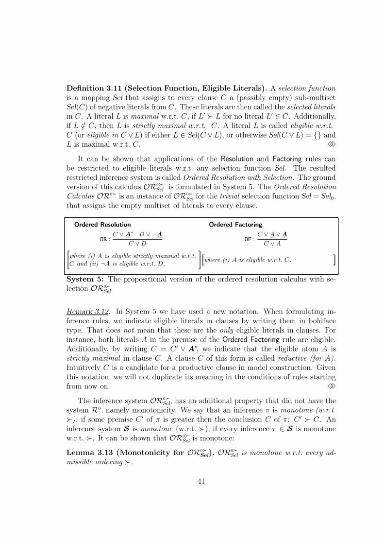
Definition 3.11 (Selection Function, Eligible Literals). A selection functionis a mapping Sel that assigns to every clause C a (possibly empty) sub-multisetSel(C) of negative literals from C. These literals are then called the selected literalsin C. A literal L is maximal w.r.t. C, if L′ � L for no literal L′ ∈ C. Additionally,if L /∈ C, then L is strictly maximal w.r.t. C. A literal L is called eligible w.r.t.C (or eligible in C ∨L) if either L ∈ Sel(C ∨L), or otherwise Sel(C ∨L) = {} andL is maximal w.r.t. C. 33

It can be shown that applications of the Resolution and Factoring rules canbe restricted to eligible literals w.r.t. any selection function Sel. The resultedrestricted inference system is called Ordered Resolution with Selection. The groundversion of this calculus OR0�

Selis formulated in System 5. The Ordered Resolution

Calculus OR0� is an instance of OR0�Sel

for the trivial selection function Sel = Sel0,that assigns the empty multiset of literals to every clause.

Ordered Resolution Ordered Factoring

OR :C ∨ A? D ∨ ¬A

C ∨ DOF :

C ∨ A ∨ A

C ∨ A

where (i) A is eligible strictly maximal w.r.t.C and (ii) ¬A is eligible w.r.t. D.

where (i) A is eligible w.r.t. C.

System 5: The propositional version of the ordered resolution calculus with se-lection OR0�

Sel

Remark 3.12. In System 5 we have used a new notation. When formulating in-ference rules, we indicate eligible literals in clauses by writing them in boldfacetype. That does not mean that these are the only eligible literals in clauses. Forinstance, both literals A in the premise of the Ordered Factoring rule are eligible.Additionally, by writing C = C ′ ∨ A?, we indicate that the eligible atom A isstrictly maximal in clause C. A clause C of this form is called reductive (for A).Intuitively C is a candidate for a productive clause in model construction. Giventhis notation, we will not duplicate its meaning in the conditions of rules startingfrom now on. 33

The inference system OR0�Sel, has an additional property that did not have the

system R0, namely monotonicity. We say that an inference π is monotone (w.r.t.�), if some premise C ′ of π is greater then the conclusion C of π: C ′ � C. Aninference system S is monotone (w.r.t. �), if every inference π ∈ S is monotonew.r.t. �. It can be shown that OR0�

Selis monotone:

Lemma 3.13 (Monotonicity for OR0�Sel

). OR0�Sel is monotone w.r.t. every ad-

missible ordering �.

41

Proof. We must show that the conclusion of the Ordered Resolution and OrderedFactoring rules from ground clauses are smaller then some premise of these rules:

(1) OR : C ∨ A?, D ∨ ¬A ` C ∨ D (Ordered Resolution):We show that the conclusion of the Ordered Resolution rule is always smaller than itsright premise. Indeed, by condition (R1) of admissible ordering (see Definition 3.4),we must have ¬A � A. Additionally, by condition (i) of this inference rule, wehave A � C. This implies (D ∨ ¬A) � (C ∨ D), what was required to show.

(2) OF : C ∨ A ∨ A ` C ∨ A (Ordered Factoring):Monotonicity of the Ordered Factoring rule is obvious, since � is monotone w.r.t.multiset inclusion of clauses: (C ∨ A ∨ A) � (C ∨ A). 22

Theorem 3.14 (Completeness of OR0�Sel

). Let N be a set of ground clauses thatis saturated in the inference system OR0�

Selbased on an admissible ordering � and

a selection function Sel. Then N is satisfiable iff N does not contain the emptyclause �.

Proof. The proof of this theorem goes in the same way as for Theorem 3.3, exceptfor a couple of moments below.

(a) We need to modify the notion of a productive clause (see Definition 3.5).A clause C ∈ N is productive w.r.t. an interpretation I if (i) I 2 C and (ii)C = C ′ ∨ A?, i.e., A is an eligible literal which is �-strictly greatest w.r.t. C ′. Inthis case, C produces A.

(b) If I 2 D but D is not productive w.r.t. I, then this is only possible if either Dis the empty clause, or (1) D = D′∨¬A (i.e., ¬A is eligible in D) for some A suchthat I �A, or there are no negative eligible literals and hence (2) D = D′ ∨A∨A(i.e., A is eligible in D but not strictly maximal). The proof of Counterexample-Reduction Lemma (Lemma 3.9). must be adjusted accordingly for these cases. Inboth cases either the Ordered Resolution rule or the Ordered Factoring rule can beapplied which reduces a counterexample. 22

In fact, ordered resolution is complete for a larger class of orderings than or-derings admissible according to Definition 3.4. Condition (W) (well-foundednessand totality) can be dropped without affecting refutational completeness. The re-sulted class of orderings is called A-orderings [Kowalski & Hayes, 1968], [see alsoChapter 5 in Fermüller et al., 1993]. We define an extension of A-orderings forground literals called L-orderings:

Definition 3.15 (L-ordering). An ordering � on ground literals is called L-ordering if:

(R1) ¬A � A for every ground atom A. 33

42

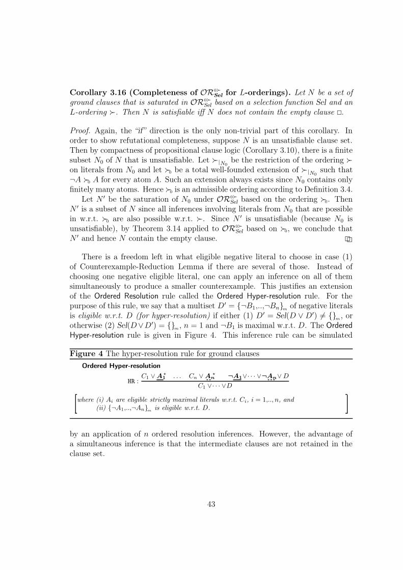
Corollary 3.16 (Completeness of OR0�Sel

for L-orderings). Let N be a set ofground clauses that is saturated in OR0�

Selbased on a selection function Sel and an

L-ordering �. Then N is satisfiable iff N does not contain the empty clause �.

Proof. Again, the “if” direction is the only non-trivial part of this corollary. Inorder to show refutational completeness, suppose N is an unsatisfiable clause set.Then by compactness of propositional clause logic (Corollary 3.10), there is a finitesubset N0 of N that is unsatisfiable. Let �|N0

be the restriction of the ordering �on literals from N0 and let �0 be a total well-founded extension of �|N0

such that¬A �0 A for every atom A. Such an extension always exists since N0 contains onlyfinitely many atoms. Hence �0 is an admissible ordering according to Definition 3.4.

Let N ′ be the saturation of N0 under OR0�Sel based on the ordering �0. Then

N ′ is a subset of N since all inferences involving literals from N0 that are possiblein w.r.t. �0 are also possible w.r.t. �. Since N ′ is unsatisfiable (because N0 isunsatisfiable), by Theorem 3.14 applied to OR0�

Sel based on �0, we conclude thatN ′ and hence N contain the empty clause. 22

There is a freedom left in what eligible negative literal to choose in case (1)of Counterexample-Reduction Lemma if there are several of those. Instead ofchoosing one negative eligible literal, one can apply an inference on all of themsimultaneously to produce a smaller counterexample. This justifies an extensionof the Ordered Resolution rule called the Ordered Hyper-resolution rule. For thepurpose of this rule, we say that a multiset D′ = {¬B1,..,¬Bn}m

of negative literalsis eligible w.r.t. D (for hyper-resolution) if either (1) D′ = Sel(D ∨ D′) 6= {}

m, or

otherwise (2) Sel(D∨D′) = {}m, n = 1 and ¬B1 is maximal w.r.t. D. The Ordered

Hyper-resolution rule is given in Figure 4. This inference rule can be simulated

Figure 4 The hyper-resolution rule for ground clauses

Ordered Hyper-resolution

HR :C1 ∨ A1

? . . . Cn ∨ An? ¬A1∨· · · ∨¬An∨ D

C1 ∨· · · ∨D

where (i) Ai are eligible strictly maximal literals w.r.t. Ci, i = 1,.., n, and(ii) {¬A1,..,¬An}m

is eligible w.r.t. D.

by an application of n ordered resolution inferences. However, the advantage ofa simultaneous inference is that the intermediate clauses are not retained in theclause set.

43

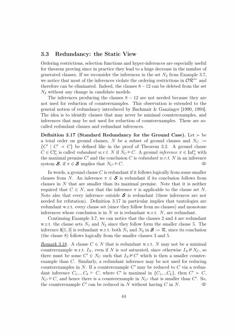
3.3 Redundancy: the Static View

Ordering restrictions, selection functions and hyper-inferences are especially usefulfor theorem proving since in practice they lead to a huge decrease in the number ofgenerated clauses. If we reconsider the inferences in the set N2 from Example 3.7,we notice that most of the inferences violate the ordering restrictions in OR0� andtherefore can be eliminated. Indeed, the clauses 8− 12 can be deleted from the setN2 without any change in candidate models.

The inferences producing the clauses 8 − 12 are not needed because they arenot used for reduction of counterexamples. This observation is extended to thegeneral notion of redundancy introduced by Bachmair & Ganzinger [1990, 1994].The idea is to identify clauses that may never be minimal counterexamples, andinferences that may be not used for reduction of counterexamples. These are so-called redundant clauses and redundant inferences.

Definition 3.17 (Standard Redundancy for the Ground Case). Let � bea total order on ground clauses, N be a subset of ground clauses and NC :={C ′ | C ′ ≺ C} be defined like in the proof of Theorem 3.2. A ground clauseC ∈ Cl0

Σis called redundant w.r.t. N if NC �C. A ground inference π ∈ Inf0

Σwith

the maximal premise C ′ and the conclusion C is redundant w.r.t. N in an inferencesystem S, if π ∈ S implies that NC′ �C. 33

In words, a ground clause C is redundant if it follows logically from some smallerclauses from N . An inference π ∈ S is redundant if its conclusion follows fromclauses in N that are smaller than its maximal premise. Note that it is neitherrequired that C ∈ N , nor that the inference π is applicable to the clause set N .Note also that every inference outside S is redundant (these inferences are notneeded for refutation). Definition 3.17 in particular implies that tautologies areredundant w.r.t. every clause set (since they follow from no clauses) and monotoneinferences whose conclusion is in N or is redundant w.r.t. N , are redundant.

Continuing Example 3.7, we can notice that the clauses 2 and 4 are redundantw.r.t. the clause sets N1 and N2 since they follow form the smaller clause 5. Theinference R[1, 3] is redundant w.r.t. both N1 and N2 in S := R, since its conclusion(the clause 8) follows logically from the smaller clauses 3 and 5.

Remark 3.18. A clause C ∈ N that is redundant w.r.t. N may not be a minimalcounterexample w.r.t. IN , even if N is not saturated, since otherwise IN 2 NC , sothere must be some C ′ ∈ NC such that IN 2 C ′ which is then a smaller counter-example than C. Similarly, a redundant inference may be not used for reducingcounterexamples in N : If a counterexample C ′ may be reduced to C via a redun-dant inference C1,.., Ck ` C, where C ′ is maximal in {C1,..,Ck}, then C ′ � C,NC′ �C, and hence there is a counterexample in NC′ that is smaller than C ′. So,the counterexample C ′ can be reduced in N without having C in N . 33

44

Redundancy notions allow one to weaken the conditions of Theorem 3.14, sothat the conclusion of this theorem still holds. We say that a clause set N issaturated up to redundancy w.r.t. an inference system S, if every S-inference π =C1,.., Ck ` C from N (i.e. when π ∈ S and Ci ∈ N , i = 1,.., k) is redundant w.r.t.N . The following is a stronger version of Theorem 3.14:

Theorem 3.19 (Completeness for OR0�Sel

-Saturated Sets up to Redun-dancy).Let N be a set of ground clauses that is saturated up to redundancy in OR0�

Selbased

on an admissible ordering � and a selection function Sel. Then N is satisfiable iffN does not contain the empty clause �.

Proof. The proof of this theorem proceeds in the same way as for Theorem 3.14.The only modification that has to be done, is the case in Counterexample-ReductionLemma, when an inference reducing a counterexample is possible but has not beenmade because of redundancy. In this case one applies the argument given in Re-mark 3.18 to find a smaller counterexample. 22

3.4 Redundancy: the Dynamic View

In order to use Theorem 3.19 effectively, one should come up with a derivationstrategy such that for every clause set N either (i) the empty clause is eventuallyderived and hence N is unsatisfiable, or otherwise, (ii) the process can be continued(forever) and a saturated set is obtained (“in the limit”). Modern saturation-basedtheorem provers implement a combination of two interleaving processes:

1. Deduction, during which conclusions of (non-redundant) inferences areproduced and

2. Deletion, during which unnecessary (redundant) clauses are removed froma clause set.

The precise definition of this process can be given using an abstract notion ofredundancy:

Definition 3.20 (Redundancy Criterion).An (abstract) redundancy criterion is a pair R = (RCl(·), RInf (·)) of functions, thatassign for every clause set N ⊆ ClΣ, a set RCl(N) ⊆ ClΣ of R-redundant clausesw.r.t. N and a set RInf (N) ⊆ InfΣ of R-redundant inferences w.r.t. N , such thatfor all sets of clauses N ′ and N with N \ N ′ ⊆ RCl(N) the following propertieshold:

(R1) if N is unsatisfiable, then N ′ is unsatisfiable;(R2) RCl(N) ⊆ RCl(N

′);(R3) RInf (N) ⊆ RInf (N

′);

45

A redundancy criterion R is effective, if in addition:

(R4) for every inference π ∈ InfΣ such that π(N) ⊆ N , we have π ∈ RInf (N).33

Conditions (R1) – (R4) for a redundancy criterion R have the following mean-ing: If a clause set N ′ is obtained from a clause set N by removing some redundantclauses and adding some other clauses, then this transformation preserves (R1):unsatisfiability of clause sets as well (R2): redundancy of clauses and (R3): re-dundancy of inferences. Finally, condition (R4) implies that an inference becomesredundant as long as its conclusion has been added to a clause set.

The trivial but effective redundancy criterion is the “smallest” R0 = (R0

Cl(·), R0Inf (·))

that admits all properties (R1) – (R4), which can be defined as follows: R0Cl(N) := {};

R0Inf (N) := {(C1,.., Ck ` C) ∈ InfΣ | C ∈ N}.

The redundancy criterion given in Definition 3.17 is called the standard redun-dancy criterion (for ground clauses) R

S�gr = (R�

Cl0(·), RS�Inf0(·)) w.r.t. an inference

system S parametrized by an ordering �. When we speak about redundancywithout mentioning R, we usually refer to this notion. We show that this redun-dancy criterion admits all properties of Definition 3.20.

Lemma 3.21 (Standard Redundancy Criterion). The notion of standardredundancy R

S�gr = (R�

Cl0(·), RS�Inf0(·)) is a redundancy criterion for ground clauses.

If in addition the inference system S is monotone, then RS�gr is effective.

Proof. For showing the properties (R1) – (R3) for RS�gr , it suffices to prove that

for every sets N , N ′ of ground clauses and a ground clause C we have thatN \ N ′ ⊆ R

�Cl0(N) implies N ′ �N and N ′

C �NC . Indeed, N ′ �N guarantees theproperty (R1). Since C ∈ R

�Cl0(N) iff NC �C, we have that N ′

C � NC implies (R2):R�Cl0(N) ⊆ R

�Cl0(N

′). Similarly, π ∈ RS�Inf0(N) iff NC′ �C for the maximal premise

C ′ of π ∈ S, so N ′C �NC implies (R3): R

S�Inf0(N) ⊆ R

S�Inf0(N

′).Note that NC \ N ′

C ⊆ R�Cl0(N) ∩ NC ⊆ R

�Cl0(NC), so it suffices to show that

N \ N ′ ⊆ R�Cl0(N) implies N ′ � N . This can be done as follows. Suppose this

property does not hold and let C be a minimal w.r.t. � clause in N such thatN ′ 2 C, so N ′ �NC . Then C ∈ N \ N ′ ⊆ R

�Cl0(N), hence NC �C and we have

obtained a contradiction N ′ � Nc � C with N ′ 2 C.To show (R4), let π ∈ S. Since S is monotone, we have C ′ � C for some

premise C ′ and the conclusion C of π. If C ∈ N or C ∈ R�Cl0(N) then NC′ � NC �C,

and so π ∈ RS�Inf0(N). 22

Remark 3.22. The proof of Lemma 3.21 uses the fact that the ordering � is well-founded, when we claim existence of a minimal w.r.t. � clause C satisfying certain

46

properties. Actually, this lemma does not hold for general L-orderings. For ex-ample, in the clause set N = {A1,¬A1, A2,¬A2, . . . , Ai,¬Ai, . . . } with ¬A1 � A1 �¬A2 � A2 � · · · , all clauses are redundant w.r.t. N (i.e., N ⊆ RCl(N)). Indeed,every clause Ai or ¬Ai with i ≥ 1, follows from the pair of smaller clauses Aj,¬Aj

with j = i + 1. So, N \ {} ⊆ RCl(N) but {}2 N , since N is inconsistent. Thisexample shows that the notion of standard redundancy is not fully compatiblewith L-orderings. However, some redundancy elimination techniques, in particu-lar, tautology deletion can be justified also for L-orderings [see Kowalski & Hayes,1968]. 33

An abstract model of a saturation procedure can be defined using the binaryrelation ⇒ on clause sets called the (theorem-proving) derivation relation ⇒, thatis defined in Figure 5 using two rules. The Deduction rule allows one to extend

Figure 5 Theorem-proving derivations “⇒” for S and R

DeductionN ⇒ N ∪ N ′ if N ′ ⊆ [S \ RInf (N)](N)

DeletionN ⇒ N \ N ′ if N ′ ⊆ RCl(N)

a clause set by adding conclusions of non-R-redundant S-inferences. Using theDeletion rule a clause set can be filtered by removing R-redundant clauses. A(finite or countably infinite) sequence N0 ⇒ N1 ⇒ N2 ⇒ · · · is called a (theorem-proving) derivation from N0 (based on S and R). The set N∞ :=

⋃i≥0

⋂j≥i Nj of

all persisting clauses is called the limit of the derivation. Sometimes we say thatN∞ is an (S,R)-saturation of N0 for the reasons that will be clear in a moment.

Lemma 3.23 (Properties of the Limit Set). Let N0 ⇒ N1 ⇒ · · · be a deriva-tion based on S and R. Then (i) if N0 is unsatisfiable then N∞ is unsatisfiable;(ii) RCl(

⋃i≥0 Ni) ⊆ RCl(N∞) and (iii) RInf (

⋃i≥0 Ni) ⊆ RInf (N∞).

Proof. Let N ′ := (⋃

i≥0 Ni). For every clause C ∈ N ′ \ N∞ there exists somei ≥ 0 such that C ∈ Ni \ Ni+1 ⊆ RCl(Ni). Indeed, otherwise either C /∈ N ′, orC ∈

⋂i≥j Nj ∈ N∞ for some j ≥ 0. By condition (R2) of redundancy criterion (see

Definition 3.20), C ∈ Ni \ Ni+1 ⊆ RCl(Ni) ⊆ RCl(N′) and so N ′ \ N∞ ⊆ RCl(N

′).Now claim (i) of the lemma follows from condition (R1) of redundancy criterion,

since N0 \ N∞ ⊆ N ′ \ N∞ ⊆ RCl(N′). Claims (ii) and (iii) follow respectively

from conditions (R2) and (R3) of redundancy criterion. 22

Definition 3.24 (Fair Derivation). A theorem-proving derivation N0 ⇒ N1 ⇒· · · based on S and R is called fairsaturation, if for every inference π ∈ S fromN∞ (i.e., when π(N∞) 6= {}), there exists some j ≥ 0 such that π is redundantw.r.t. Nj. 33

47

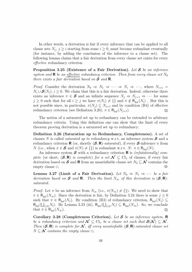
In other words, a derivation is fair if every inference that can be applied to allclause sets Nj, j ≥ i starting from some i ≥ 0, must become redundant eventually(for instance, by adding the conclusion of the inference to a clause set). Thefollowing lemma claims that a fair derivation from every clause set exists for everyeffective redundancy criterion.

Proposition 3.25 (Existence of a Fair Derivation). Let S be an inferencesystem and R be an effective redundancy criterion. Then from every clause set N0

there exists a fair derivation based on S and R.

Proof. Consider the derivation N0 ⇒ N1 ⇒ · · · ⇒ Ni ⇒ · · · , where Ni+1 =Ni ∪S(Ni), i ≥ 0. We claim that this is a fair derivation. Indeed, otherwise thereexists an inference π ∈ S and an infinite sequence Nj ⇒ Nj+1 ⇒ · · · for somej ≥ 0 such that for all i ≥ j we have π(Ni) 6= {} and π /∈ RInf (Ni) . But this isnot possible since, in particular, π(Nj) ⊆ Nj+1 and by condition (R4) of effectiveredundancy criterion (see Definition 3.20), π ∈ RInf (Nj+1). 22

The notion of a saturated set up to redundancy can be extended to arbitraryredundancy criteria. Using this definition one can show that the limit of everytheorem proving derivation is a saturated set up to redundancy:

Definition 3.26 (Saturation up to Redundancy, Completeness). A set ofclauses N is called saturated up to redundancy w.r.t. an inference system S and aredundancy criterion R (or, shortly (S,R)-saturated), if every S-inference π fromN (i.e., when π ∈ S and π(N) 6= {}) is redundant w.r.t. N : π ∈ RInf (N).

An inference system S with a redundancy criterion R is (refutationally) com-plete (or short, (S,R) is complete) for a set N ⊆ ClΣ of clauses, if every fairderivation based on S and R from an unsatisfiable clause set N0 ⊆ N contains theempty clause �. 33

Lemma 3.27 (Limit of a Fair Derivation). Let N0 ⇒ N1 ⇒ · · · be a fairderivation based on S and R. Then the limit N∞ of this derivation is (S,R)-saturated.

Proof. Let π be an inference from N∞ (i.e., π(N∞) 6= {}). We need to show thatπ ∈ RInf (N∞). Since the derivation is fair, by Definition 3.24 there is some j ≥ 0such that π ∈ RInf (Nj). By condition (R3) of redundancy criterion, RInf (Nj) ⊆RInf (

⋃i≥0 Ni). By Lemma 3.23 (iii), RInf (

⋃i≥0 Ni) ⊆ RInf (N∞). So, we conclude

that π ∈ RInf (N∞). 22

Corollary 3.28 (Completeness Criterion). Let S be an inference system, R

be a redundancy criterion and N ⊆ ClΣ be a clause set such that S(N ) ⊆ N .Then (S,R) is complete for N , iff every unsatisfiable (S,R)-saturated clause setN ⊆ N contains the empty clause �.

48

Proof. The “only if ” part of the corollary is simple: If (S,R) is complete for N andN ⊆ N is an unsatisfiable (S,R)-saturated clause set, then the trivial derivationconsisting only of N is fair: all S-inferences from N are R-redundant w.r.t. N .Hence, from completeness of (S,R), we obtain that N contains the empty clause�.

To prove the “if ” part, suppose that (S,R) is not complete. Then there exists afair derivation N0 ⇒ N1 ⇒ · · · from an unsatisfiable clause set N0 ⊆ N based on Sand R such that � /∈ Ni for every i ≥ 0. Note that for every i ≥ 0, we have Ni ⊆ N .Hence the limit N∞ of the derivation is a subset of N . By Lemma 3.23 (i), N∞ isunsatisfiable, since N0 is unsatisfiable. Moreover, N∞ ⊆

⋃i≥0 Ni, hence � /∈ N∞.

But this is not possible, since by Lemma 3.27, N∞ is (S,R)-saturated, and by ourassumption, � ∈ N∞. 22

Remark 3.29. Note that the “only if ” part of Corollary 3.28, holds without theassumption that S(N ) ⊆ N . 33

Corollary 3.30 (Completeness for OR0�Sel

with Redundancy). (OR0�Sel

, RS�gr )

is complete for the set Cl0Σ

of ground clauses.

Proof. By Theorem 3.19, every (OR0�Sel, R

S�gr )-saturated unsatisfiable subset N ⊆

Cl0Σ

of ground clauses contains the empty clause �. Hence the corollary is a conse-quence of Corollary 3.28 because OR0�

Sel(Cl0Σ) ⊆ Cl0Σ. 22

Note 3.31. Definitions of redundancy criteria and fair derivations vary in literature.Our definition of redundancy criteria is equivalent to the one given in [Bachmair& Ganzinger, 2001]. This definition can be weaken, in particular condition (R2)can be replaced with condition (R2)′: “N ⊆ N ′ implies RCl(N) ⊆ RCl(N

′)”, so thatLemma 3.27 still holds. For an even weaker definition of redundancy criterion see[Bachmair, Ganzinger & Waldmann, 1994].

We have also strengthened the definition of fair derivation, compared to the onegiven in [Bachmair & Ganzinger, 2001; Bachmair et al., 1994], since it appears tobe more handy for showing fairness of saturation strategies that we describe in sec-tion 7). In this form it is more close to the definition of fairness given in [Nieuwen-huis & Rubio, 2001]. The weakest, although completely useless definition wouldbe to say that a derivation is fair if N∞ is (S,R)-saturated. 33

A limit of a theorem proving derivation for a given clause set N0 is not uniquein general. Even a finite clause set may have several different minimal satura-tions w.r.t. the standard redundancy criterion, as demonstrates the example below.However for the trivial redundancy criterion R

0, the saturation is always uniqueand consists of all clauses S∗(N0) that are derivable from the initial clause set, asno deletion step takes place.

49

Example 3.32. Let � be an admissible ordering such that ¬A � A � ¬B � B �¬C � C. Consider the clause set N0 := {¬AA?, AA?∨ C, BB ∨ BB, BB?∨ ¬C}. This clauseset has two derivations based on OR0� and R

S�gr that produce different minimal

saturated set up to redundancy given in Figure 6. The (non-redundant) inferencesthat can be applied to N0 are OR[2; 1] and OF[3]. Depending on the order in whichthese inferences are applied we obtain two different derivations.

Figure 6 Computing saturated sets with redundancy

N0 : {①

¬AA?,②

AA?∨ C,③

BB ∨ BB,④

BB?∨ ¬C}⇓ OR[2;1]

N1 : {①

¬AA?,②

AA?∨ C,③

BB ∨ BB,④

BB?∨ ¬C,⑤

CC?}⇓ DelRed

N2 : {①

¬AA?,④

BB?∨ ¬C,⑤

CC?}

N0 : {①

¬AA?,②

AA?∨ C,③

BB ∨ BB,④

BB?∨ ¬C}⇓ OF[3]

N ′1 : {

①

¬AA?,②

AA?∨ C,③

BB ∨ BB,④

BB?∨ ¬C,⑥

BB?}⇓ DelRed

N ′2 : {

①

¬AA?,②

AA?∨ C,⑥

BB?}⇓ OR[2;1]

N ′3 : {

①

¬AA?,②

AA?∨ C,⑥

BB?,⑤

CC?}⇓ DelRed

N ′4 : {

①

¬AA?,⑥

BB?,⑤

CC?}

In the first derivation, we have applied inference OR[2; 1] which produced clause5. CC?. This clause renders clause 2 redundant since the last clause contains literalC. Moreover, clause 3 and hence inference OF[3] become redundant w.r.t. N1 sinceclause 3 follows from the smaller clauses 4 and 5. After we delete all redundantclauses in N1 (2 and 3 are the only clauses in N1 that are redundant w.r.t. N1),we obtain a clause set N2 which is saturated in OR0� (up to redundancy), sinceno further inferences apply.

If we apply inference OF[3] first (see the right derivation in Figure 6), we obtainclause 6. BB?, which renders clauses 3 and 4 redundant. After the deletion step,inference OR[2; 1] remains possible, and at the end, a different saturated set N ′

4 isproduced. 33

One can argue that the set N ′4 is a “better” saturated set than the set N2, since

N2 \N ′4 ⊆ RCl(N

′4) but not vice versa. Note that the clause 6 can be obtained from

the clauses 4 and 5 by applying an (unordered) resolution inference. The result ofthis inference, i.e., the clause 6 makes the clause 4 redundant. This inference isan instance of a so-called Subsumption Resolution inference rule [see Bachmair &Ganzinger, 2001]. To allow such useful inferences, a calculus is usually enhancedwith additional simplification rules. We return to this point in section 7.

50

3.5 Lifting

By Lifting Lemma (Lemma 2.42), every clause set N represents the set of itsground instances N gr (here represents means “is equisatisfiable with”). Hence, forlifting a refutationally complete calculus from ground clauses it suffices to finda sound inference system for general clauses such that for every set N that issaturated w.r.t. this system, the set of its ground instances N gr is saturated w.r.t.the ground calculus.

In this section we describe the lifted version OR� of the ordered resolutioncalculus, and in the next section, we show how selection functions can be integratedinto this model. To describe OR�, we need to “lift” the ordering restrictions fromthe ground calculus OR0�.

Definition 3.33 (Liftable Orders, Lifting). An order � on expressions is calledliftable if there exists an order �0 on ground expressions such that E1 � E2 impliesthat E1σ�0 E2σ for every ground substitution σ. The lifting of an order � definedon ground expressions is a liftable order containing � (which we denote by thesame letter) that is defined as follows: E1 � E2 iff for every ground substitutionσ it holds that E1σ � E2σ. 33

Note that the lifting of a total order on ground expressions may not be a to-tal order: two unifiable different expressions (e.g., p(x, c) and p(c, x)) may notbe comparable by �, since they have a common instance. To give another ex-ample, consider an LPO-ordering based on the precedence f � p � q � c (seeDefinition 2.19). The atoms p(x, x) and q(y) are not comparable by �lpo, sincep(c, c) �lpo q(c), but q(f(c)) �lpo p(c, c). On the other hand, p(x, y) �lpo q(y) andq(f(x)) �lpo p(x, x). From Example 2.22, it also follows that q(f(x)) �kbo p(x, x)never holds.

An order � on atoms is usually extended to literals by setting ¬A � A �¬B � B for all atoms A � B. By LPO (or KBO) order on literals we mean thisextension of the respective lifted orders from ground clauses.

Definition 3.34 (Admissible Orders for Ordered Resolution). An order �on literals is called admissible for resolution, if (i) � is liftable and (ii) � isadmissible for ground literals according to Definition 3.4. 33

Note that by this definition, an admissible order should be total on groundliterals. Recall, that a literal L is maximal w.r.t. a clause C, if L′ � L for noliteral L′ ∈ C. If in addition L /∈ C, then L is called strictly maximal w.r.t. C.The lifted version of the Ordered Resolution calculus OR� (without selection) isgiven in System 6. The inference rules are applied to clauses whose variables arerenamed apart , so that they do not have variables in common. This can be alwaysdone, since all variables in clauses are implicitly universally quantified. The ordered

51

Ordered Resolution Ordered Factoring

OR :C ∨ A? D ∨ ¬B

Cσ ∨ DσOF :

C ∨ B ∨ A

Cσ ∨ Aσ

where (i) σ = mgu(A, B); (ii) Aσ is strictly maximalw.r.t. Cσ and (iii) ¬Bσ is maximal w.r.t. Dσ

where (i) σ = mgu(A, B); (ii) Aσ ismaximal w.r.t. Cσ ∨ Bσ.

System 6: The ordered resolution calculus OR�

resolution calculus OR� defines a sound inference system, since it is a restrictionof resolution calculus R, which is sound (see Remark 3.1).

Inference rules of System 6 are organized in such a way that, if an orderedresolution inference is possible from some ground instances of clauses, then theinference should be possible from these (non-ground) clauses that captures theresult of the ground inference (see Figure 7).

Figure 7 The lifting diagram for OR�

OR�:

OR0�:

C ∨ A?, D ∨ ¬B Cσ ∨ Dσ

C0 ∨ A0?, D0 ∨ ¬A0 C0 ∨ D0

__

gr��

__

gr

��

OR+3

OR +3

C ∨ B ∨ A Cσ ∨ Aσ

C0 ∨ A0 ∨ A0

C0 ∨ A0

__

gr

��

__

gr

��

OF+3

OF +3

The way how the ordering restrictions (ii) and (iii) are applied in the conditionsof OR�-inference rules in System 6, is called a-posteriori , i.e., after an inferenceis made. This way the inferences are more restrictive than with a-priori orderingrestrictions, i.e., for σ = id. The a-priori ordering restrictions for the inferencerules of OR� are indicated by our notation for (strictly maximal) eligible literals(see Remark 3.12).

Remark 3.35. Note that even a-posteriori ordering restrictions do not guaranteethat there is always a ground instance of the respective inference that satisfies theordering restrictions. For example, a simple inference:

OR :a(x, x) ∨ cc(xx, yy)? ¬cc(uu, vv) ∨ ¬b(v, v)

a(x, x) ∨ ¬b(y, y)(15)

with the unifier σ := {u/x, v/y}, satisfies all a-posteriori (and a-priori) orderingrestrictions of the ordered resolution rule for KBO-ordering �kbo based on a prece-dence with a � b � c. However, for any inference from ground instances of thepremises of (15):

OR :a(s0, s0) ∨ cc(s0, t0)? ¬cc(s0, t0) ∨ ¬b(t0, t0)

a(s0, s0) ∨ ¬b(t0, t0)(16)

52

we must have weight(t0) > weight(s0) from the ordering restrictions for the leftpremise, and weight(s0) > weight(t0)weight from the restrictions for the rightpremise, which is not possible. Hence, the inference rule (15) has no ground in-stances. 33

The problem spotted in Example 3.35 can be addressed using an extension ofthe standard redundancy criterion (see Definition 3.17) for general clauses:

Definition 3.36 (Standard Redundancy). Let � be an admissible order ac-cording to Definition 3.34. A clause C is redundant w.r.t. N (notation: C ∈R�Cl(N)), if every ground instance Cσ of C is redundant w.r.t. N gr (according to

Definition 3.17). An inference π = C1,.., Ck ` C is redundant w.r.t. N (in S)(notation: π ∈ R

S�Inf (N)), if every ground instance πσ := C1σ,.., Ckσ ` Cσ (i.e.,

when all Ciσ with i = 1,.., k and Cσ are ground), is redundant w.r.t. N gr in S 0,where S 0 is the restriction of S to ground clauses. 33

Note that an instance πσ may be not an inference of S 0 even if π ∈ S, sincethe unified expressions might not match, or ordering restrictions may be violated.For example, the inference (15) in Remark 3.35 has no valid ground instances. Inthis case the inference π is vacuously redundant, since all its ground inferences arenot in S 0 and hence redundant (see remark after Definition 3.17). Inferences thatare outside S are redundant as well, since according to the lifting diagram (seeFigure 7) they may not have valid ground instances.

Lemma 3.37 (Standard Redundancy Criterion). The notion of standard re-dundancy R

S� = (R�Cl(·), R

S�Inf (·)) given in Definition 3.36 is a redundancy criterion

for general clauses ClΣ. In addition, if S 0 is monotone, then RS� is effective.

Proof. Lemma 3.37 is a consequence of Lemma 3.21 since by Definition 3.36, forevery clause sets N ′ and N , we have N ⊆ R

�Cl(N) iff Ngr ⊆ R

�Cl0(N

gr), and for

every set of inferences S, we have S ⊆ RS�Inf (N) iff Sgr ⊆ R

S0�Inf0 (Ngr), where Sgr is

the set of all ground instances of inferences in S. 22

To demonstrate a non-trivial case of redundant inferences, we consider an ex-ample from [Nieuwenhuis & Rubio, 2001], that shows how resolution inferencesbetween transitivity axioms can be avoided.

Example 3.38. Consider the set consisting of the single clause T : ¬p(x, y) ∨¬p(y, z) ∨ p(x, z) that expresses the transitivity axiom for p: “p(x, y) and p(y, z)implies p(x, z)”. Let � be some admissible ordering that is a rewrite ordering forground expressions (see subsection 2.4, p. 21), say KBO or LPO ordering.

Every negative literal of T is maximal in T, since it is maximal in its instancewhere all variables are replaced by the same ground term. For many orderings �

53

(again, in particular for KBO or LPO), the positive literal is also maximal, hencethe Ordered Resolution rule can be applied to (two copies of) T:

OR :¬p(x, y) ∨ ¬p(y, z) ∨ pp(xx, zz)? ¬pp(uu, vv) ∨ ¬p(v, w) ∨ p(u, w)

¬p(x, y) ∨ ¬p(y, z) ∨ ¬p(z, w) ∨ p(x, w)(17)

with the unifier is σ := {u/x, v/z}. The conclusion of this inference is the clause:

OR[T; T] : T′. ¬p(x, y) ∨ ¬p(y, z) ∨ ¬p(z, w) ∨ p(x, w);

which can be seen as a weak transitivity axiom. For similar reasons as for T, theclause T′ can be further resolved with T producing even longer clauses:

OR[T′ ; T] : T′′ . ¬p(x, y) ∨ ¬p(y, z) ∨ ¬p(z, u) ∨ ¬p(u, w) ∨ p(x, w);OR[T′′; T] : T′′′. ¬p(x, y) ∨ ¬p(y, z) ∨ ¬p(z, u) ∨ ¬p(u, v) ∨ ¬p(v, w) ∨ p(x, w);

. . . etc.Now we show how the notion of redundancy can be used to avoid all these

dangerous inferences. First we show that the clause T′ is not always redundantw.r.t. the clause set {T} when the inferences above are possible.

Consider any LPO ordering �lpo and suppose that the clause T′ is redundantw.r.t. {T}. By Definition 3.36, this in particular means that the following groundinstance of T′ :

T′0. ¬p(s0, r0) ∨ ¬pp(r0, t0)?∨ ¬p(t0, h0) ∨ p(s0, h0) (18)

with r0 �lpo s0 �lpo t0 �lpo h0, follows from the set {T′}grT′0

of smaller groundinstances of T. We claim that {T′}gr

T′0contains either the left clause from (19) or

the left clause from (20) below:

¬p(s0, r0) ∨ ¬p(r0, t0) ∨ p(s0, t0); ¬p(s0, t0) ∨ ¬p(t0, h0) ∨ p(s0, h0); (19)

¬p(r0, t0) ∨ ¬p(t0, h0) ∨ p(r0, h0); ¬p(s0, r0) ∨ ¬p(r0, h0) ∨ p(s0, h0). (20)

Indeed, otherwise I0 := {p(s0, r0), p(r0, t0), p(t0, h0)} is a model of {T′}grT′0

: the onlyinstances of T in which both negative literals are false are the left clauses from (19)and (20), which we assume to be not in {T′}gr

T′0. But I0 is not a model of T′0, hence

T′0 does not follow from {T′}grT′0

.On the other hand, none of these left clauses may be in {T′}gr

T′0, because they

are �lpo-greater than T′0, since p(s0, t0) �lpo ¬p(t0, h0)∨ p(s0, h0) and p(r0, h0) �lpo

¬p(s0, r0)∨p(s0, h0). Hence T′0 does not follow from {T′}grT′0

and so T′ is not redundantw.r.t. {T}.

Although the clause T′ is not redundant w.r.t. {T}, it is possible to show thatinference (17) that has produced T′, is redundant w.r.t. {T} for every monotone

54

admissible ordering � that is total on ground terms.7 To show redundancy, ac-cording to Definition 3.36, we should consider arbitrary ground instance (19) ofthe Ordered Resolution inference (17) that produces instance (18) of the conclusionof this inference (we discard the LPO-ordering considered before). We need todemonstrate that clause (18) follows from some instances of T that are smallerthan the maximal premise of this ground inference, namely the right clause from(19). We show that the clauses from (20) are those instances that we need.

Obviously, clause (18) is a consequence of (20). What remains to be shown, isthat both clauses from (20) are smaller than the right clause from (19). To provethis, we use the conditions of the Ordered Resolution rule that is applied to (19).The ordering restrictions for the left premise yield: p(, t0) � ¬p(, r0) � p(, r0) andp(, t0) � ¬p(r0, t0) � p(r0, t0). By monotonicity and totality of � on ground terms,we obtain that t0 � r0 and � r0. This together with the ordering restrictions forthe right premise yield ¬p(, t0) � ¬p(t0, h0) � ¬p(r0, h0) � p(r0, h0). Now it iseasy to check that the right clause from (19) is �-larger than both clauses from(20). Hence, the inference (17) is redundant w.r.t. {T}.

Similarly, it can be shown that the resolution inference with the second negativeliteral of T is redundant. Here we need to consider an arbitrary instance (20) of theordered resolution inference and, using the ordering restrictions demonstrate, thatthe conclusion of this inference can be obtained by (unordered) resolution from thesmaller clauses (19). 33

It is hard to come up with a general algorithm using which redundancy ofclauses and inferences can be shown. In the Saturate system [Ganzinger, Nieuwen-huis & Nivela, 2002], some concrete techniques for proving redundancy are imple-mented. For the particular example above with �=�lpo, this prover finds redun-dancy automatically by employing clausal rewriting combined with LPO constraintsolving. In [Kazakov, 2005] we demonstrate how the proof model described in Ex-ample 3.38 can be adapted to obtain decision procedures for variety of non-trivialfragments of first-order logic with transitive predicates and related theories.

The notion of saturation up to redundancy (see Definition 3.26) can be appliedto the ordered resolution calculus OR� with the (extended) standard redundancycriterion from Definition 3.36. Our goal now is to show refutational completenessof this calculus.

Theorem 3.39 (Completeness of OR� with Redundancy). (OR�, RS�) isrefutationally complete for ClΣ.

Proof. Since RS� is a redundancy criterion (see Lemma 3.37), by the completeness

criterion (see Corollary 3.28), it suffices to show that every unsatisfiable set N that

7In [Nieuwenhuis & Rubio, 2001] redundancy of this inference has been shown only for LPO

55

is saturated in OR� up to redundancy, contains the empty clause �. Furthermore,it suffices to prove that (i) if N is (OR�, RS�)-saturated then N gr is (OR0�, RS�

gr )-saturated. Indeed, this together with (ii) N is unsatisfiable implies that N gr isunsatisfiable and (iii) � /∈ N implies that � /∈ N gr, yield a contradiction if � /∈ N ,since (OR0�, RS�

gr ) is complete (see Corollary 3.30).The fact (i) is a consequence of the following two lemmas that follow directly

from the introduced definitions:

Lemma 3.40. For every clause C 0 ∈ Ngr, there exists a clause in C ∈ N suchthat C 0 is a ground instance of C and for every literal L0 that is (strictly) maximalin C 0, the correspondent literal L in C is (strictly) maximal in C.

Lemma 3.41. For every inference π0 = C 01 ,.., C

0k ` C 0 ∈ OR0� from Ngr there

exists an inference π = C1,.., Ck ` C ∈ OR� from N , such that π0 is an instanceof π. Moreover, if π is redundant w.r.t. N then π0 is redundant w.r.t. N gr. 22

3.6 Selection Functions for General Clauses

Selection functions can be extended to clauses with variables in the same wayas given in Definition 3.11, that is a selection function Sel selects a sub-multisetSel(C) of negative literals in every clause C. To integrate selection functionsinto OR� as it is done for OR0�

Sel, we extend the notion of eligible literals (see

Definition 3.11) as follows: Given a clause C and a substitution σ, we say that aliteral L is eligible (strictly maximal) w.r.t. C and σ if either L ∈ Sel(C ∨ L), orotherwise Sel(C ∨ L) = {} and Lσ is (strictly) maximal w.r.t. Cσ. The OrderedResolution calculus with selection OR�

Sel parametrized by a selection function Seland an admissible ordering � is given in System 7.

Ordered Resolution Ordered Factoring

OR :C ∨ A? D ∨ ¬B

Cσ ∨ DσOF :

C ∨ B ∨ A

Cσ ∨ Aσ

where (i) σ = mgu(A, B); (ii) A is eligible strictlymaximal w.r.t. C and σ and (iii) ¬B is eligiblew.r.t. D and σ.

where (i) σ = mgu(A, B); (ii) A iseligible w.r.t. C and σ.

System 7: The ordered resolution calculus with selection OR�Sel

There are some technical difficulties in proving refutational completeness of theordered resolution with selection functions. In particular, the calculus in System 7is no longer compatible with the lifting diagram in Figure 7, since the selectedliterals in a clause and its ground instances may not correspond. It is possible to

56

fix this problem by allowing only “liftable” selection functions in similar way howit is done for orderings. However this is not desirable in practice, where a selectionfunctions are used to control the behaviour of a saturation procedure, like in theexample below.

Example 3.42. To demonstrate the problems that arise with arbitrary selectionfunctions, consider the clause set

N0 = {pp(xx, ff(xx))?, qq(xx, ff(xx))?, ¬p(x, y) ∨ ¬qq(xx, xx)], ¬pp(xx, xx)]∨ ¬q(x, y)}.

First, it is reasonable to set the selection function Sel to select the negative literalswith one variable in the last two clauses, since this ensures that no inferences canbe drawn between the clauses (here and further we mark selected literals by ]).Now, the question is, what should be selected in clause ¬p(c, c) ∨ ¬q(c, c), whichis a common ground instance of the last two clauses? Regardless which selectionfunction we choose, the lifting diagram in Figure 7 will not work: If literal ¬p(c, c)becomes eligible in this ground instance, then the inference between clauses p(x, x)and ¬p(x, y)∨¬qq(xx, xx)] is not possible, although it is possible between its groundinstances p(c, c) and ¬pp(cc, cc) ∨ ¬q(c, c). The situation when literal ¬q(c, c) iseligible in clause ¬p(c, c) ∨ ¬q(c, c) is symmetric.

However for the fixed clause set N , it is always possible to extend the selectionfunction to ground literals such that every inference between clauses from N gr

will correspond to some inferences between clauses from N . This idea is used forproving completeness of OR�

Sel with non-liftable selection functions. Please find inAppendix A.1 the details of the proof. 33

There are other related technical problems with general selection functions, inparticular, how to define the notion of redundant inferences. This is also discussedin Appendix A.1. Using techniques discuss in this appendix, it is possible to justifyso-called subsumption deletion:

Definition 3.43 (Subsumption). A clause C subsumes a clause D (or D issubsumed by C) if Cσ ⊆ D for some substitution σ (the inclusion between clausesis the inclusion between their multisets of literals). A clause C strictly subsumes aclause D (D is strictly subsumed by C) if C subsumes D but D does not subsumeC. 33

For example, the clause a(x) ∨ a(y) subsumes the clauses a(x) ∨ a(x), a(y) ∨a(x)∨a(c), a(f(x))∨a(c), but not, say the clause a(x) or the clause a(f(x)). Notealso that clauses which subsume each other are variants of each other.

It is possible to extend the notion of redundancy in such a way that clausesthat are strictly subsumed by C are redundant w.r.t. C and hence can be deletedduring a saturation process. For details, please see Appendix A.2.

57

3.7 Hyper-Resolution Strategies

The extension of ground resolution calculus with the hyper-inference given inFigure 4 can be lifted in a similar way. To formulate the resulted inference system,we say that a multiset D′ = {¬B1,..,¬Bn}m

of negative literals is eligible w.r.t. Dand σ (for hyper-resolution) if either (a) D′ = Sel(D ∨ D′) 6= {}

m, or, otherwise

(b) Sel(D ∨ D′) = {}m, n = 1 and ¬B1σ is maximal w.r.t. Dσ. Now the Ordered

Hyper-Resolution calculus with selection HR�Sel

is defined by replacing the OrderedResolution rule with the Ordered Hyper-resolution rule given in Figure 8.

Figure 8 The hyper-resolution rule

Ordered Hyper-resolution

HR :C1 ∨ A1

? . . . Cn ∨ An? ¬B1∨· · · ∨¬Bn∨ D

C1σ ∨· · · ∨Dσ

where (i) σ = mgu({A1=B1, . . . , An=Bn}); (ii) Aiσ are eligible strictly maximal w.r.t. Ci

and σ, i = 1,.., n and (iii) {¬B1,..,¬Bn}mis eligible w.r.t. D and σ.

The hyper-resolution rule can be further extended to a more powerful rule witha-posteriori selection strategy, which has been employed in [de Nivelle & de Ri-jke, 2003] for deciding the loosely guarded fragment. This rule can be describedusing the a-posteriori selection function Sela that assigns to a unification problemP = {A1=B1,.., An=Bn} between first-order atoms, its non-empty subproblem:Sela(P) ⊆ P, Sela(P) 6= {}. The extended Ordered Hyper-resolution is given inFigure 9.

Figure 9 The hyper-resolution rule with a-posteriori selection

Ordered Hyper-resolution

HR :C1 ∨ A1

? . . . Ck ∨ Ak? . . . Cn ∨ An

? ¬B1∨· · · ∨¬Bk ∨· · · ∨¬Bn ∨ D

C1τ ∨· · · ∨¬Bk+1τ ∨· · · ∨¬Bnτ ∨ Dτ

where (i) σ = mgu({A1=B1, . . . , An=Bn}); (ii) Ai are eligible strictly maximal w.r.t. Ci andσ, 1 ≤ i ≤ n; (iii) {¬B1,..,¬Bn}m

is eligible w.r.t. D and σ; (iv) Sela({A1=B1,.., An=Bn}) ={A1=B1,.., Ak=Bk} and (v) τ = mgu({A1=B1,.., Ak=Bk}).

58

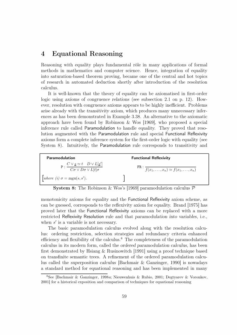
4 Equational Reasoning

Reasoning with equality plays fundamental rôle in many applications of formalmethods in mathematics and computer science. Hence, integration of equalityinto saturation-based theorem proving, became one of the central and hot topicsof research in automated deduction shortly after introduction of the resolutioncalculus.

It is well-known that the theory of equality can be axiomatised in first-orderlogic using axioms of congruence relations (see subsection 2.1 on p. 12). How-ever, resolution with congruence axioms appears to be highly inefficient. Problemsarise already with the transitivity axiom, which produces many unnecessary infer-ences as has been demonstrated in Example 3.38. An alternative to the axiomaticapproach have been found by Robinson & Wos [1969], who proposed a specialinference rule called Paramodulation to handle equality. They proved that reso-lution augmented with the Paramodulation rule and special Functional Reflexivityaxioms form a complete inference system for the first-order logic with equality (seeSystem 8). Intuitively, the Paramodulation rule corresponds to transitivity and

Paramodulation Functional Reflexivity

P :C ∨ s ' t D ∨ L[s′]

Cσ ∨ Dσ ∨ L[t]σFR :

f(x1, . . . , xn) ' f(x1, . . . , xn)

where (i) σ = mgu(s, s′).

System 8: The Robinson & Wos’s [1969] paramodulation calculus P

monotonicity axioms for equality and the Functional Reflexivity axiom scheme, ascan be guessed, corresponds to the reflexivity axiom for equality. Brand [1975] hasproved later that the Functional Reflexivity axioms can be replaced with a morerestricted Reflexivity Resolution rule and that paramodulation into variables, i.e.,when s′ is a variable is not necessary.

The basic paramodulation calculus evolved along with the resolution calcu-lus: ordering restriction, selection strategies and redundancy criteria enhancedefficiency and flexibility of the calculus.8 The completeness of the paramodulationcalculus in its modern form, called the ordered paramodulation calculus, has beenfirst demonstrated by Hsiang & Rusinowitch [1991] using a proof technique basedon transfinite semantic trees. A refinement of the ordered paramodulation calcu-lus called the superposition calculus [Bachmair & Ganzinger, 1990] is nowadaysa standard method for equational reasoning and has been implemented in many

8See [Bachmair & Ganzinger, 1998a; Nieuwenhuis & Rubio, 2001; Degtyarev & Voronkov,2001] for a historical exposition and comparison of techniques for equational reasoning

59

systems such as Vampire [Riazanov & Voronkov, 2002], Spass [Weidenbach etal., 2002], E [Schulz, 2002] and Bliksem [de Nivelle, 1998a].

In this section we review the ordered paramodulation calculus OP�Sel and the

superposition calculus SP�Sel

. We present completeness proofs for these calculi ac-cording to the general model construction schema demonstrated for the resolutioncalculus. Although the superposition calculus is more restrictive than the para-modulation calculus, the last can be still used for deciding certain shallow clauseclasses, for example the one for the guarded fragment [see Kazakov, 2005].

4.1 The Ordered Paramodulation Calculus

The ordered paramodulation calculus OP�Sel is an extension of the ordered resolution

calculus OR�Sel

with two rules given in System 9. Like ordered resolution, thiscalculus is parametrized by an ordering � on literals and a selection functionSel, but the ordering � is now extended also to terms. In order to simplify the

Ordered Paramodulation Reflexivity Resolution

OP :C ∨ s ' t? D ∨ L[s′]

Cσ ∨ Dσ ∨ L[t]σRR :

C ∨ s 6' s′

Cσ

where (i) σ = mgu(s, s′); (ii) s ' t is eligible strictlymaximal w.r.t. C and σ; (iii) L[s′] is eligible (strictlymaximal if positive) w.r.t. D and σ; (iv) (sσ ' tσ) 6�L[s′]σ; (v) tσ 6� sσ and (vi) s′ is not a variable.

where (i) σ = mgu(s, s′) and (ii) s 6's′ is eligible w.r.t. C and σ.

System 9: The ordered paramodulation calculus OP�Sel

exposition of calculi with equality, we identify every non-equational atom A ∈ At−Σ

with the equation A ' T (and its negation with A 6' T), where T is some fixedconstant, which intuitively stands for “True”. This allows us to deal only withequational atoms of the form E1 ' E2 over two sorts of expressions E1, E2 ∈At−Σ t TmΣ.

Definition 4.1 (Admissible Order). An ordering � is admissible for parmodu-lation if � is admissible for resolution (see Definition 3.34) and additionally:

(T) � is total on ground terms with the least element T;(E1) t ≺ s C L implies L[s] � L[t] (monotonicity);(E2) t ≺ s C E1 implies (E1[s] ' E2) � (s ' t); 33

Condition (T) and (E1) of admissible ordering together with (L) from Defi-nition 3.4 imply that � is a total reduction ordering on ground expressions (seep. 21). Condition (E2) ensures that an equational atom s ' t used in a paramo-dulation inference is always smaller than the atom into which paramodulation is

60

performed, except, perhaps, for equational atoms of the form s ' h with s � t � h.In this case the last atom can be paramodulated into the first. Note that since �is liftable, it suffices to require conditions (E1) – (E2) for ground expressions only.

An admissible ordering for paramodulation can be obtained, for example, bytaking the lifting of any total reduction ordering � on ground terms and non-equational ground atoms, like KBO or LPO, extended to equational literals bytreating every positive literal E1 ' E2 as the multiset {E1, E2}m

and every negativeliteral E1 6' E2 as the multiset {E1, E1, E2, E2}m

.It is easy to show that Ordered Paramodulation and Reflexivity Resolution are

sound and that the restriction of OP�Sel

to ground clauses forms a monotone infer-ence system:

Lemma 4.2 (Monotonicity for OP�Sel

). OP�Sel

is monotone for ground clausesw.r.t. every admissible ordering �.

Proof. Monotonicity of the Ordered Resolution and Ordered Factoring rules has beenalready shown in Lemma 3.13 (recall that every ordering � that is admissible forparamodulation is also admissible for resolution). It remains to show monotonicityof the Ordered Paramodulation and Reflexivity Resolution rules:

(1) OP : C ∨ s ' t?, D ∨ L[s] ` C ∨ D ∨ L[t] (Ordered Paramodulation):We show that the conclusion of the Ordered Paramodulation rule is always smallerthan the right premise of this rule. Indeed, by conditions (iv) and (ii) of this rule,we must have L[s] � (s ' t) � C. By condition (v) of this rule and condition (E1)of admissible ordering, we have L[s] � L[t]. Hence, D∨L[s] � (C ∨D∨L[t]) whatwas required to show.

(2) RR : C ∨ s 6' s ` C (Reflexivity Resolution):This inference rule is obviously monotone since � is monotone w.r.t. multisetinclusion. 22

The standard redundancy criterion RS� = (R�

Cl(·), RS�Inf (·)) is extended to equa-

tional calculi without new surprises. As usual, we say that a ground clause C 0 isredundant w.r.t. a set of ground clauses N 0, if C 0 follows from N 0

C0 . A groundinference π0 is redundant w.r.t. N 0 in OP 0�

Sel′ if either π0 /∈ OP 0�

Sel′ or, otherwise,

the conclusion of π0 follows from N 0C0

ifor some premise C 0

i of π0. Note, that “fol-lows” here means in the theory of equality. We will often say that such redundancycriterion is based on semantical entailment , in this case in equational theory.

A (general) clause C is redundant w.r.t. a clause set N if every ground instanceC 0 ∈ {C}gr of C is redundant w.r.t. N gr. An inference π is redundant w.r.t. N inOP�

Sel, if every ground instance π0 of π is redundant w.r.t. N gr in OP0�

Sel′ for every

projection Sel′ of Sel from the premises of π.

61

4.1.1 Refutational completeness for the ground clauses

In this section we consider the restriction OP 0�Sel of the ordered paramodulation

calculus OP�Sel

to the ground clauses Cl0Σ. Unless stated otherwise, all terms and

clauses in this section are ground.We extend the model construction given in subsection 3.1 to the paramodula-

tion calculus. Given a set of ground clauses N that is saturated (up to redundancy),we are going to construct a candidate model IN for N . Every model that we con-struct in our procedure is represented by a set of oriented ground equational atomsI, which form a rewrite system: E1 ' E2 with E1 � E2 is read as E1 ⇒E2. The(rewrite) model induced by I is denoted by I⇓ and is defined by setting an atomA = (E1 ' E2) to be true in I⇓ (notation: I⇓�A) iff the equation E1 ' E2

converges w.r.t. ⇒I , i.e., the expressions E1 and E2 are I-joinable: E1 ⇓I E2 (recallthe notations and definitions from subsection 2.3). In particular, a non-equationalatom A ∈ At−Σ is true in I⇓, iff A⇓I = T.

The interpretation I⇓ is equational only if the underlying rewrite system isconvergent. By Critical Pair Lemma (Lemma 2.11), a rewrite system is convergentif and only if it is terminating and confluent. Termination of I is guaranteed bythe ordering �, since every admissible ordering is well-founded. Confluence of Iwill be implied from a stronger property:

Definition 4.3 (Canonical Rewrite System). Given an atom A and a set ofatoms I, let IA (IA) denote a set of atoms from I that are smaller (resp. smalleror equal) than A. We say that an atom A = (E1 ' E2) is irreducible w.r.t. I ifboth E1 and E2 are irreducible w.r.t. I. A rewrite system (= set of atoms) I iscanonical (for paramodulation) if every atom A from I is irreducible w.r.t. IA. 33

It will be shown below that every canonical rewrite system is confluent. Inaddition, canonical rewrite systems admit a nice property, namely that for provingan equation E1 ' E2, it suffices to use only those rewrite rules that are not greaterthan this equation:

Lemma 4.4 (Canonical Proofs). Let I be a canonical rewrite system. Then(i) I is confluent and (ii) for every atom A := (E1 ' E2), we have I⇓�A iffIA⇓�A.

Proof. (i) In order to show that I is confluent, let A = (E1 ⇒ E2) and A′ =

(E ′1 ⇒E ′

2) be two different overlapping rewrite rules from I with E ′1 E E1, then

either (a) E ′1 C E1 and hence A � A′ (by condition (E2) of admissible ordering),

which means that A is reducible w.r.t. IA, or (b) E1 = E ′1 and either A is reducible

w.r.t. IA (if A � A′), or A′ is reducible w.r.t. IA′ (if A′ � A). Both cases are notpossible since I is canonical.

62

(ii) The “if ” part of this case is trivial since IA ⊆ I. To show the “onlyif ” part, we employ induction on A over the well-ordered set (At0

Σ,�). Recall,

that I⇓�(E1 ' E2) iff E1 ⇓I E2. If both expressions in E1 and E2 from A areirreducible w.r.t. I, then E1 = E2, and the lemma is trivial, which provides thebasis of induction.

W.l.o.g. assume that expression E1 is reducible by some rewrite rule (E ′1 ⇒ E ′

2) ∈

I. If A � (E ′1 ⇒ E ′

2), then by the induction hypothesis, the equation (E1[E′1/E

′2] '

E2) ≺ A (by condition (E1)) is true in IA⇓, and so IA⇓� A, which was requiredto show.

Now suppose that A ≺ (E ′1 ⇒E ′

2). Since E ′1 E E1, this is only possible if

E ′1 = E1, because of condition (E2) for admissible orderings. For similar reasons,

E ′2 � E2 and E ′

2 is irreducible w.r.t. I (otherwise it is reducible by some rewriterule that is smaller than E ′

1 ⇒ E ′2, which is not possible since I is canonical). Hence

E1⇓I = E ′2 � E2 and the equation E1 ' E2 cannot converge. Therefore this case

is not possible. 22

Now we describe a model construction for the paramodulation calculus.

Definition 4.5 (Productive Clause). A clause C is productive w.r.t. a set ofatoms I, if (i) I⇓2 C; (ii) C = C ′ ∨A, where A = (E1 ' E2) is an eligible strictlygreatest atom w.r.t. C ′ and E1 � E2,9 and (iii) A is irreducible w.r.t. I. In thiscase we say that C produces a rewrite rule ∆IC := (E1 ⇒ E2) w.r.t. I. If C is notproductive, we assign ∆IC := {}. 33

Definition 4.6 (Candidate Models). Let N ⊆ Cl0Σ

and C ∈ Cl0Σ. The candidate

models for N , NC and NC are induced respectively by the sets IN , IC and IC thatare defined as follows:IN :=

⋃C∈N

IC ; IC :=⋃

C′∈NC

IC′

, and IC := IC ∪ ∆C, where ∆C := ∆ICC. 33

Lemma 4.7 (Properties of Candidate Models). Let N be a clause set forwhich candidate models are constructed according to Definition 4.6. Then for everyC ∈ N , (i) IC⇓�C implies that IN⇓�C and (ii) If C = (C ′ ∨ A?) is productivew.r.t. IC then IN⇓2 C ′.

N Clauses C ∆C

C C ′ ∨ ¬B ?

Proof. (i) If IC⇓� A for some positive atom A in C, thenIN⇓� A �C. Otherwise, C should contain negatively someatom B such that IC⇓2 B, but IN⇓�B. This situation isnot possible, since by Lemma 4.4, IB⇓� B, but IB ⊆ IC 2 B, since B ≺ ¬B � C(by condition (R1) of admissible ordering).

9Note that E1 = E2 is already not possible by condition (i), hence the maximal atom in Ccan be always oriented

63

N Clauses C ∆C

C

C ′︷ ︷C ′′ ∨ B ∨ A? A

(ii) Assume that for some productive clause C = (C ′ ∨ A?),we have IN⇓� C ′. First, note that IC⇓2 C ′ since C is aproductive clause. Hence there exists an atom B whichoccurs positively in C ′, and becomes true in IN⇓. SinceIN forms a canonical rewrite system (by condition (iii) of productive clause), byLemma 4.4 (ii), IB⇓�B. Since C � A � B, we have IC⇓� IB⇓�B �C ′. Acontradiction. 22

Lemma 4.8 (Counterexample-Reduction Lemma). Let N be a set of groundclauses which is saturated w.r.t. OP�

Sel up to redundancy. Then for every clauseD ∈ N with IN⇓2 D 6= �, there exists D1 ∈ N such that D1 ≺ D and IN⇓2 D1.

Proof. Let IN⇓2 D for some clause D ∈ N . Then ID⇓2 D, since otherwise byLemma 4.7 (i) we would have IN⇓�D. In particular, clause D cannot be pro-ductive. So, we have ID⇓ = ID⇓2 D. According to the definition of productiveclauses (see Definition 4.14), this situation is possible only in the following cases:

N Clauses C ∆C

D D′ ∨ s 6' s −gD1 D′ ?

(1) D = (D′∨¬A) for some eligible literal ¬A in D, and ID⇓� A = (E1 ' E2).W.l.o.g. assume that E1 � E2. Then either (1.1) E1 = E2 =s for some ground term s ∈ Tm0

Σ, or (1.2) the atom A is

reducible w.r.t. ID.In case (1.1), the Reflexivity Resolution rule can be applied

to D that produces a smaller clause RR[D]: D1 = D′ ∈ Nthan D which is false in IN⇓.

N Clauses C ∆C

D D′ ∨ ¬A[s] −g

D1 C ′ ∨ D′ ∨ ¬A[t] ?

C C ′ ∨ s ' t? s⇒ t

In case (1.2), A must be reducible by some rewriterule produced by a clause C = (C ′ ∨ B) ≺ D. If this is aterm rewrite rule B = (s⇒ t), then the Ordered Paramo-dulation rule can be applied to C and D that producesa clause OP[C, D]: D1 = (C ′ ∨ D′ ∨ ¬A[t]) ∈ N whichis smaller counterexample than D. If B = (P ⇒ T), where P is a non-equationalatom, then A = (P ⇒ T), hence the Ordered Resolution rule can be applied to Cand D that produces a clause OR[C, D]: D1 = (C ′ ∨ D′) ∈ N which is again asmaller counterexample than D.

(2) D = (D′ ∨A∨A), where A is an eligible greatest literal in D. In this case,the Ordered Factoring rule is applied to D that produces a clause OF[D]: D1 =(D′ ∨ A) ∈ N which is a smaller counterexample than D. 22

Counterexample-Reduction Lemma implies completeness of the ground orderedparamodulation calculus:

Theorem 4.9 (Completeness of OP0�

Selwith Redundancy).

(OP 0�Sel

, RS�) is complete for the set Cl0Σ

of ground clauses.

64

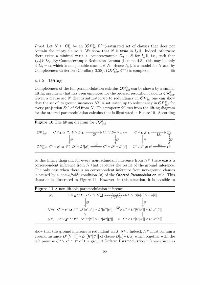
Proof. Let N ⊆ Cl0Σ be an (OP0�Sel, R

S�)-saturated set of clauses that does notcontain the empty clause �. We show that N is true in IN⇓. Indeed, otherwisethere exists a minimal w.r.t. � counterexample D0 ∈ N for IN⇓, i.e., such thatIN⇓2 D0. By Counterexample-Reduction Lemma (Lemma 4.8), this may be onlyif D0 = �, which is not possible since � /∈ N . Hence IN⇓ is a model for N and byCompleteness Criterion (Corollary 3.28), (OP 0�

Sel, RS�) is complete. 22

4.1.2 Lifting

Completeness of the full paramodulation calculus OP�Sel can be shown by a similar

lifting argument that has been employed for the ordered resolution calculus OR�Sel

.Given a clause set N that is saturated up to redundancy in OP�

Sel one can showthat the set of its ground instances N gr is saturated up to redundancy in OP 0�

Sel′ for

every projection Sel′ of Sel from N . This property follows from the lifting diagramfor the ordered paramodulation calculus that is illustrated in Figure 10. According

Figure 10 The lifting diagram for OP�Sel

OP�Sel

:

OP0�Sel′

:

C ∨ s ' t?, D ∨ L[s′] Cσ ∨ Dσ ∨ L[t]σ

C0 ∨ s0 ' t0?, D0 ∨ L0[s0] C0 ∨ D0 ∨ L0[t0]

__

gr��

__

gr��

OP+3

OP +3

C ∨ s 6' s′ Cσ

C0 ∨ s0 6' s0 C0

__

gr

��

__

gr

��

RR+3

RR +3

to this lifting diagram, for every non-redundant inference from N gr there exists acorrespondent inference from N that captures the result of the ground inference.The only case when there is no correspondent inference from non-ground clausesis caused by a non-liftable condition (v) of the Ordered Paramodulation rule. Thissituation is illustrated in Figure 11. However, in this situation, it is possible to

Figure 11 A non-liftable paramodulation inference

N :

Ngr:

Ngr:

ooooooo OOOOOOOC ∨ s ' t?, D[x] ∨ L[x] C ∨ D[h[s]] ∨ L[h[t]]

C0 ∨ s0 ' t0?, D0[h0[s0]] ∨ L0[h0[s0]] C0 ∨ D0[h0[s0]] ∨ L0[h0[t0]]

C0 ∨ s0 ' t0?, D0[h0[t0]] ∨ L0[h0[t0]] C0 ∨ D0[h0[s0]] ∨ L0[h0[t0]]

g

�

__

gr��

__

gr��

OP+3

OP +3

show that this ground inference is redundant w.r.t. N gr. Indeed, Ngr must contain aground instance D0[h0[t0]]∨L0[h0[t0]] of clause D[x]∨L[x] which together with theleft premise C 0 ∨ s0 ' t0 of the ground Ordered Paramodulation inference implies

65

the conclusion of this inference. Since both of these clauses are smaller thenthe maximal clause D0[h0[s0]] ∨ L0[h0[s0]] of the inference (because s0 � t0), thisinference is redundant according to the standard redundancy criterion. Hence thelifting diagram in Figure 10 holds (recall, that correspondence must be establishedonly for non-redundant inferences).

Theorem 4.10 (Completeness of OP�

Selwith Redundancy). (OP�

Sel, RS�)

is complete.

Similar usage of redundancy can also justify a very useful refinement of theOrdered Paramodulation rule with simultaneous paramodulation: see Figure 12. In

Figure 12 The simultaneous ordered paramodulation rule

(Simulteneous) Ordered Paramodulation

OP :C ∨ s ' t? D[s′] ∨ L[s′]

Cσ ∨ D[t]σ ∨ L[t]σ

where (i) σ = mgu(s, s′); (ii) s ' t is eligible strictly maximal w.r.t. C and σ; (iii) L[s′] iseligible (strictly maximal if positive) w.r.t. D and σ; (iv) (sσ ' tσ) 6� L[s′]σ; (v) tσ 6� sσand (vi) s′ is not a variable.

this rule, paramodulation is simultaneously performed into several occurrences ofthe term s′ in the right premise. It can be shown that the usual paramodula-tion inference becomes redundant as long as the conclusion of the simultaneousparamodulation inference has been drawn:

ooooooo OOOOOOOC ∨ s ' t?, D[s] ∨ L[s] C ∨ D[s] ∨ L[t]

C ∨ s ' t?, C ∨ D[t] ∨ L[t] C ∨ D[s] ∨ L[t]�

OP +3

OP (Simult.) g��

(21)

The simulteneous paramodulation inference rule can be realized through an ad-ditional selection function, that given a clause, its literal and a subterm in thisliteral, selects some other occurrences of this subterm in this clause. The rulemust be applied on all selected subterms in the clause. For the purpose of ourdecision procedures, we will use the full selection, i.e., we will apply simultaneousparamodulation rule on all subterms s′ in the right premise.

4.2 The Superposition Calculus

We can notice some similarity between the ordered paramodulation calculus andthe ordered Knuth-Bendix completion procedure described in subsection 2.3 in

66

System 2. Both saturation procedures result in an equational model that is rep-resented by a convergent rewrite system. However the Superposition rule is morerestricted then the Ordered Paramodulation rule in that the former rewrites onlythe largest term of an equational atom. The ideas behind the Knuth-Bendix com-pletion and the paramodulation calculus have been joined into the superpositioncalculus that has been first introduced in [Bachmair & Ganzinger, 1990]. The su-perposition calculus SP�

Selis an extension of the ordered resolution calculus OR�

Sel

with inference rules given in System 10. Instead of a single Ordered Paramodula-

Ordered Paramodulation

OP :C ∨ s ' t? D ∨ L[s′]

Cσ ∨ Dσ ∨ L[t]σ

where (i) σ = mgu(s, s′); (ii) s ' t is eligible strictly maximal w.r.t. C and σ; (iii) L[s′] iseligible (strictly maximal if positive) w.r.t. D and σ; (iv) L[s′] is a non-equational literal;(v) tσ 6� sσ and (vi) s′ is not a variable.

Positive Superposition Negative Superposition

PS :C ∨ s ' t? D ∨ r[s′] ' h

?

Cσ ∨ Dσ ∨ r[t]σ ' hσNS :

C ∨ s ' t? D ∨ r[s′] 6' h?

Cσ ∨ Dσ ∨ r[t]σ 6' hσ

where (i) σ = mgu(s, s′); (ii) s ' t is eligiblestrictly maximal w.r.t. C and σ; (iii) r ' his eligible strictly maximal w.r.t. D and σ;(iv) (sσ ' tσ) 6� (rσ ' hσ); (v) tσ 6� sσ;(vi) hσ 6� rσ and (vii) s′ is not a variable.

where (i) σ = mgu(s, s′); (ii) s ' t is eligiblestrictly maximal w.r.t. C and σ; (iii) r 6' his eligible strictly maximal w.r.t. D and σ;(iv) tσ 6� sσ; (v) hσ 6� rσ and (vi) s′ is not avariable.

Reflexivity Resolution Equality Factoring

RR :C ∨ s 6' s′

CσEF :

C ∨ s′ ' h ∨ s ' t?

Cσ ∨ tσ 6' hσ ∨ s′σ ' hσ

where (i) σ = mgu(s, s′) and (ii) s 6' s′ iseligible w.r.t. C and σ.

where (i) σ = mgu(s, s′); (ii) s ' t is eligiblestrictly maximal w.r.t. C ∨ s′ ' h and σ, and(iii) tσ 6� sσ.

System 10: The superposition calculus SP�Sel

tion rule now we have three inference rules: the Ordered Paramodulation rule intonon-equational literals, the Positive Superposition rule for paramodulation into themaximal term of positive equations and the Negative Superposition rule for para-modulation into the maximal term of negative equations.10 Additionally we havea new inference rule Equality Factoring whose rôle will be revealed in a moment.

10Ordered Paramodulation into non-equational literals is often described as an instance of Pos-itive Superposition or Negative Superposition when atoms are viewed as equations over two sortsof expressions

67

Note that a restriction of the superposition calculus to positive unit equationalatoms is our well-known ordered Knuth-Bendix completion procedure.

In order to prove refutational completeness for the superposition calculus SP�Sel,

we modify the model construction given for the paramodulation calculus OP�Sel

. Itseems like we only need to relax the condition (iii) from the definition of productiveclause (see Definition 4.5), such that the maximal non-equational expression of themaximal atom A in a clause C is irreducible w.r.t. a current rewrite system. If weaccept this definition, we obtain a rewrite system which has the following property:

Definition 4.11 (Canonical Rewrite System). A rewrite system I is canonical

(for superposition) if for every rule A = (E1 ⇒E2) ∈ I, the expression E1 isirreducible w.r.t. IA. 33

An analog of Lemma 4.4 can be proven for rewrite systems that are canonicalfor superposition. For this we need to introduce additional notation. Given anexpression E, let IE denote the set of atoms from I whose expressions are notgreater than E: IE := {(E1 ' E2) ∈ I | E1 � E, E2 � E}. Then the followingproperty holds:

Lemma 4.12 (Canonical Proofs). Let I be a canonical rewrite system. Then(i) I is confluent and (ii) for every atom A := (E1 ' E2) with E1 � E2, we haveI⇓�A iff IE1⇓�A.

Proof. The proof for case (i) of this lemma is identical to the one for Lemma 4.4.Case (ii) follows from the fact that every expression involved in a rewrite proof forA := (E1 ' E2) is not greater then the maximal expression from {E1, E2}. 22

Unfortunately an analog of Lemma 4.7 does not hold if candidate models areconstructed according to the modified procedure above. This is demonstrated inthe following example:

N Clauses C ∆C

1. a 6' c ∨ aa 6' bb −

2. a ' c ∨ aa ' bb? a⇒ b:::::

3. bb ' cc? b⇒ c

Example 4.13. Let � be an ordering such that a �b � c. Consider a clause set N shown in the tableto the right. Clauses 1 – 3 from N are arranged indecreasing order w.r.t. �. Clause 3 produces a rewriterule b⇒ c. Although the maximal atom a ' b ofclause 2 is reducible w.r.t. to this rewrite rule, itsmaximal term a is not. Hence, clause 2 produces a rewrite rule a⇒ b. But nowthe remaining literal a ' c of this clause becomes true in I2 and consequently inIN . Hence, the important property (ii) of candidate models (see Lemma 4.7) isviolated (if this property does not hold, then an inference between a productiveclause and a counterexample might produce a clause that is true in a candidatemodel).

68

This example also demonstrates why the Equality Factoring rule is needed. It iseasy to see that the clause set N is unsatisfiable. Indeed, the empty clause can bederived from N in the paramodulation calculus: clauses 2, 3 produce a ' c andclauses 1, 3 produce a 6' c ∨ a 6' c by applying Ordered Paramodulation inferencesinto b and the Ordered Factoring rule. The rest inferences are straightforward.However the only possible superposition inferences from N are Negative Superpo-sition between clause 2 and 1 and Equality Factoring from 2. The first inferenceproduces a tautology. Hence, an empty clause cannot be derived from N withoutthe Equality Factoring rule if deletion of tautoloties is allowed.11 33

In order to retain the properties of productive clauses, we modify the notion ofproductive clause such that the situation described in Example 4.13 becomes notpossible:

Definition 4.14 (Productive Clause). A clause C is productive clause w.r.t.set of atoms I, if (i) I⇓2 C; (ii) C = C ′ ∨ A, where A = (E1 ' E2) is aneligible strictly greatest atom w.r.t. C ′ with E1 � E2; (iii) E1 is irreducible w.r.t.I and (iv) (I ∪ {E1 ⇒ E2})⇓2 C ′. In this case C produces a rewrite rule ∆IC :=

(E1 ⇒E2) w.r.t. I. If C is not productive, then we assign ∆IC := {}. 33

For proving remaining technical lemmas, we need two additional requirementsfor orderings which may be used in the superposition calculus.

Definition 4.15 (Admissible Order). An ordering � is admissible for superpo-sition if � is admissible for paramodulation (see Definition 4.1) and addittionally:

(E3) s � t � h implies (s 6' h) � (s ' t), and(E4) s � t � h implies (s ' t) � (t 6' h). 33

Condition (E3) for equational atoms plays a similar role as condition (R1) fornon-equational atoms. Condition (E4) is needed to ensure monotonicity of theEquality Factoring rule:

Lemma 4.16 (Monotonicity for SP�

Sel). SP�

Sel is monotone for ground clausesw.r.t. every admissible ordering �.

Proof. Ordered Paramodulation, Positive Superposition and Negative Superpositionare restrictions of the Ordered Paramodulation rule from the paramodulation cal-culus, which is proved to be monotone. The Reflexivity Resolution rule is left un-changed. It remains to show monotonicity of the Equality Factoring rule.

11However, this example does not imply that the Equality Factoring rule is strictly necessarywhen tautologies are not deleted. In fact, Bachmair & Ganzinger [1997] proved that a variant ofsuperpostion calculus without Equality Factoring called the strict superposition calculus , remainscomplete. To prove this, they formulated a waker notion of redundancy and used basic strategiesin order to avoid superposition into variables

69

(1) EF : C ∨ s ' h ∨ s ' t? ` C ∨ t 6' h ∨ s ' h (Equality Factoring):From conditions (ii) and (iii) of this rule, we have (s ' t) � (s ' h), and s � t,which implies (by totality and monotonicity of �) that t � h. Using condition(E4) of admissible orderings (see Definition 4.15), we obtain: (s ' t) � (t 6' h).Hence, (C ∨ s ' h ∨ s ' t) � (C ∨ t 6' h ∨ s ' h) what was required to show. 22

Lemma 4.17 (Properties of Candidate Models). Let N be a set of groundclauses. Then for every C ∈ N , (i) IC⇓�C implies that IN⇓�C and (ii) IfC = (C ′ ∨ A?) is productive w.r.t. IC then IN⇓2 C ′.

N Clauses C ∆C

C C ′ ∨ ¬B ?

Proof. (i) If IC⇓� A for some positive atom A in C, thenIN⇓� A �C. Otherwise, C should contain negatively someatom B = (E ' E ′) such that IC⇓2 B, but IN⇓�B. SinceE 6= E ′, w.l.o.g. we can assume that E � E ′. Then by Lemma 4.12, IE⇓�B.But for every atom (E1 ⇒ E2) ∈ IE, we have E � E1 � E2, and so C � ¬B =(E 6' E ′) � (E1 ' E2) by conditions (E1) and (E3) of admissible orderings. HenceIE⇓� IC⇓2 B, which contradicts to IE⇓�B.

N Clauses C ∆C

C

C ′︷ ︷C ′′ ∨ B ∨ A? A

(ii) Assume that for some productive clause C = (C ′ ∨ A?),we have IN⇓� C ′. Since IC⇓2 C ′, there must be some pos-itive atom B in C ′ that is true in IN⇓. Since IN⇓ iscanonical for superposition, then by Lemma 4.12 we haveIE � B, where E is the maximal non-equational expression in B. If B is a non-equational atom, then this situation is not possible, since IE⇓ = IB⇓ ⊆ IC⇓2 C ′.So B = (s ' h) for some ground terms s � h (s 6= h, since IC⇓2 B).

N Clauses C ∆C

D1 D′ ∨ s ' t? s⇒ tg

C C ′′ ∨B︷ ︷

s ' h ∨

A︷ ︷s ' t′ ? s⇒ t′

Since Is⇓� B but IC⇓2 B, there is a minimalproductive clause of the form D1 = (D′

1 ∨ (s 't)) � C such that ID

1 ⇓� B. Since B = (s 'h) ≺ A � (s ' t), then A must be an atom ofthe form (s ' t′), with s � t′. But the term sin (s ' t) must be irreducible w.r.t. ID1 by condition (iii) of productive clause(see Definition 4.14). This is only possible when D1 = C. So, IC⇓ = (IC ∪

{s⇒ t′})⇓�B = (s ' h) �C ′. This situation is not possible by condition (iv) ofproductive clause from Definition 4.14. 22

Lemma 4.18 (Counterexample-Reduction Lemma). Let N be a set of groundclauses which is saturated w.r.t. SP�

Sel up to redundancy. Then for every clauseD ∈ N with IN⇓2 D 6= �, there exists D1 ∈ N such that D1 ≺ D and IN⇓2 D1.

Proof. Let IN⇓2 D for some clause D ∈ N . Then ID⇓2 D, since otherwise byLemma 4.17 (i) we would have IN⇓�D. In particular, clause D cannot be pro-ductive. So, we have ID⇓ = ID⇓2 D. According to the definition of productiveclauses (see Definition 4.14), this situation is possible only in the following cases:

70

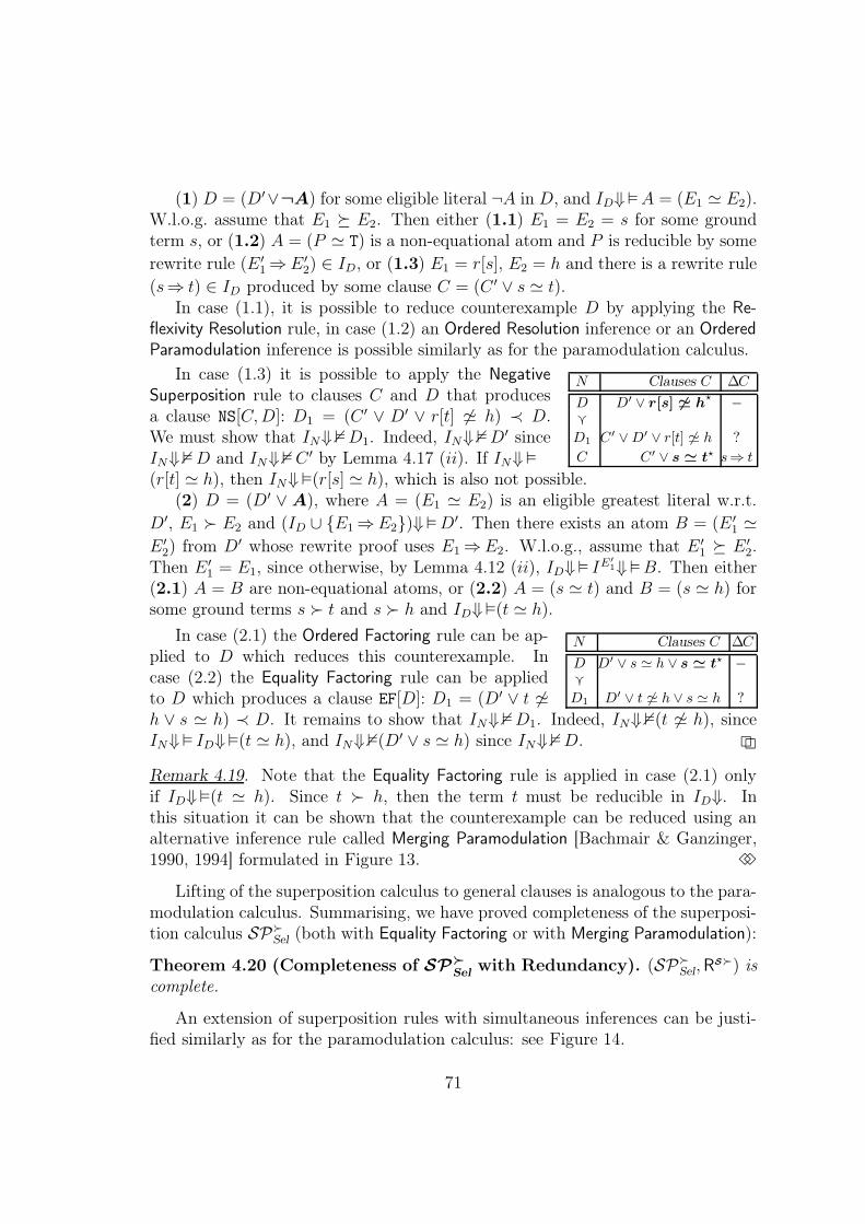
(1) D = (D′∨¬A) for some eligible literal ¬A in D, and ID⇓� A = (E1 ' E2).W.l.o.g. assume that E1 � E2. Then either (1.1) E1 = E2 = s for some groundterm s, or (1.2) A = (P ' T) is a non-equational atom and P is reducible by somerewrite rule (E ′

1 ⇒ E ′2) ∈ ID, or (1.3) E1 = r[s], E2 = h and there is a rewrite rule

(s⇒ t) ∈ ID produced by some clause C = (C ′ ∨ s ' t).In case (1.1), it is possible to reduce counterexample D by applying the Re-

flexivity Resolution rule, in case (1.2) an Ordered Resolution inference or an OrderedParamodulation inference is possible similarly as for the paramodulation calculus.

N Clauses C ∆C

D D′ ∨ r[s] 6' h?

−g

D1 C ′ ∨ D′ ∨ r[t] 6' h ?

C C ′ ∨ s ' t? s⇒ t

In case (1.3) it is possible to apply the NegativeSuperposition rule to clauses C and D that producesa clause NS[C, D]: D1 = (C ′ ∨ D′ ∨ r[t] 6' h) ≺ D.We must show that IN⇓2 D1. Indeed, IN⇓2 D′ sinceIN⇓2 D and IN⇓2 C ′ by Lemma 4.17 (ii). If IN⇓�

(r[t] ' h), then IN⇓�(r[s] ' h), which is also not possible.(2) D = (D′ ∨ A), where A = (E1 ' E2) is an eligible greatest literal w.r.t.

D′, E1 � E2 and (ID ∪ {E1 ⇒E2})⇓� D′. Then there exists an atom B = (E ′1 '

E ′2) from D′ whose rewrite proof uses E1 ⇒E2. W.l.o.g., assume that E ′

1 � E ′2.

Then E ′1 = E1, since otherwise, by Lemma 4.12 (ii), ID⇓� IE′

1⇓�B. Then either(2.1) A = B are non-equational atoms, or (2.2) A = (s ' t) and B = (s ' h) forsome ground terms s � t and s � h and ID⇓�(t ' h).

N Clauses C ∆C

D D′ ∨ s ' h ∨ s ' t? −gD1 D′ ∨ t 6' h ∨ s ' h ?

In case (2.1) the Ordered Factoring rule can be ap-plied to D which reduces this counterexample. Incase (2.2) the Equality Factoring rule can be appliedto D which produces a clause EF[D]: D1 = (D′ ∨ t 6'h ∨ s ' h) ≺ D. It remains to show that IN⇓2 D1. Indeed, IN⇓2(t 6' h), sinceIN⇓� ID⇓�(t ' h), and IN⇓2(D′ ∨ s ' h) since IN⇓2 D. 22

Remark 4.19. Note that the Equality Factoring rule is applied in case (2.1) onlyif ID⇓�(t ' h). Since t � h, then the term t must be reducible in ID⇓. Inthis situation it can be shown that the counterexample can be reduced using analternative inference rule called Merging Paramodulation [Bachmair & Ganzinger,1990, 1994] formulated in Figure 13. 33

Lifting of the superposition calculus to general clauses is analogous to the para-modulation calculus. Summarising, we have proved completeness of the superposi-tion calculus SP�

Sel(both with Equality Factoring or with Merging Paramodulation):

Theorem 4.20 (Completeness of SP�

Selwith Redundancy). (SP�

Sel, RS�) is

complete.

An extension of superposition rules with simultaneous inferences can be justi-fied similarly as for the paramodulation calculus: see Figure 14.

71

Figure 13 The merging paramodulation rule

Merging Paramodulation

MP :C ∨ s ' t? D ∨ u ' v ∨ r ' h[s′]

?

Cσ ∨ Dσ ∨ rσ ' h[t]σ ∨ uσ ' vσ

where (i) σ = mgu({s=s′, r=u}); (ii) s ' t is eligible strictly maximal w.r.t. C and σ;(iii) r ' h is eligible strictly maximal w.r.t. D ∨ u ' v and σ; (iv) tσ 6� sσ; (v) hσ 6� rσand (vi) s′ is not a variable.

Figure 14 The simultaneous superposition rules

(Simulteneous) Positive Superposition (Simulteneous) Negative Superposition

PS :C ∨ s ' t? D[s′] ∨ r[s′] ' h[s′]

?

Cσ ∨ D[t]σ ∨ r[t]σ ' h[t]σNS :

C ∨ s ' t? D[s′] ∨ r[s′] 6' h[s′]?

Cσ ∨ D[t]σ ∨ r[t]σ 6' h[t]σ

where (i) σ = mgu(s, s′); (ii) s ' t is eligiblestrictly maximal w.r.t. C and σ; (iii) r ' his eligible strictly maximal w.r.t. D and σ;(iv) (sσ ' tσ) 6� (rσ ' hσ); (v) tσ 6� sσ;(vi) hσ 6� rσ and (vii) s′ is not a variable.

where (i) σ = mgu(s, s′); (ii) s ' t is eligiblestrictly maximal w.r.t. C and σ; (iii) r 6' his eligible strictly maximal w.r.t. D and σ;(iv) tσ 6� sσ; (v) hσ 6� rσ and (vi) s′ is not avariable.

5 Chaining Calculi

The ordered paramodulation and ordered resolution calculi are examples of calculimodulo theory, in these cases – the theory of equality. The advantage of calculiwith built-in equality over direct treatment of equational axioms, is that the proofsearch for the first is restricted to a relatively narrow class of proofs, namely therewrite proofs. This basic idea can be further extended to capture some theoriesthat are weaker than equational theories. Below, we revisit specialised chainingcalculi for transitive and compositional binary relations that have been introducedby Bachmair & Ganzinger [1995, 1998b]. Using an extension of the model construc-tion method from the previous sections, we prove completeness of these calculi fora quite general class of orderings, which will play essential rôle in the decision pro-cedures that we are going to present. Among other things, we will discuss necessityfor special Transitivity Factoring and Compositional Resolution rules in chaining cal-culi which can be seen as non-symmetric analogs of the Equality Factoring rule.We also describe a particular hyper-inference strategy, and extend the standardredundancy criterion to suit a larger class of compositional theories.

72

5.1 Reasoning with Transitive Relations

In calculi with built-in theory, we have two types of signature elements: the in-terpreted (or special) symbols whose interpretation is restricted in a theory, andthe remaining free symbols. In chaining calculi we will have only binary predicatesymbols as special symbols. We have already used one special predicate symbol,namely equality ', which can be easily distinguished from others because of itsinfix notation s ' t, i.e., when the predicate symbol is situated between the ar-guments. We continue this tradition, and will use the infix notation sSt for allspecial binary predicate symbols S. We say special atoms or special literals forthose atoms or literals that contain special predicate symbols.

Since we will talk about calculi with build-in theories, we will do all logicalreasoning modulo theory as well. We say that a clause (set) is T -satisfiable (hereT denotes a theory), if it has a T -model , i.e., a model which admits all axioms ofT . The entailment relation modulo theory is denoted by T�. The notion of standardredundancy based on semantical entailment is also extended to theories. We saythat a ground clause C 0 (or a ground inference π0) is T -redundant w.r.t. a set ofground clauses N 0, if N 0

C0 T� C 0 (respectively, N 0C0

1T�C 0, where C 0

1 is the maximalpremise of π0). Redundancy of non-ground clauses and inferences is defined asusual, by considering their eligible ground instances. It will be usually the casethat a theory is known from the context, so we will often say “redundant” insteadof “T -redundant”.

In this section we consider a theory of transitivity T in which some specialpredicates T are restricted to admit the transitivity property:

xTy ∧ yTz→xTz (Transitivity) (22)

Equality is a transitive symmetric reflexive relation that admits monotonicity prop-erty. A transitive relation should behave similar to equality, except that it is neithersymmetric, nor reflexive or monotone. Using this observation, we try to obtain aspecialised calculus for transitive relation from the superposition calculus, by re-moving symmetry, reflexivity and monotonicity of the equality predicate ' fromthis calculus.

By modifying the Positive Superposition and Negative Superposition inferencerules we arrive to the inference rules given in Figure 15. The Ordered Chaining ruleis obtained from the Positive Superposition rule, by removing symmetry and mono-tonicity of equality, so that a sound inference rule for transitive relations remains.The Negative Chaining rule is similarly obtained from the Negative Superpositionrule, however, now we have two variants of rules since the transitive relation mightnot be symmetric and we must distinguish chaining into the left argument fromthe chaining into the right argument.

73

Figure 15 Ordered chaining rules for transitive relations

Ordered Chaining

OC :C ∨ tTs? D ∨ s′Tt′?

Cσ ∨ Dσ ∨ tσT t′σ

where (i) σ = mgu(s, s′); (ii) tT s is eligible strictly maximal w.r.t. C and σ; (iii) s′T t′ iseligible strictly maximal w.r.t. D and σ; (iv) tσ 6� sσ and (v) t′σ 6� s′σ.

Negative Chaining

NC :C ∨ sT t? ¬(s′Th) ∨ D

Cσ ∨ ¬(tσThσ) ∨ Dσ

C ∨ tTs? ¬(hTs′) ∨ D

Cσ ∨ ¬(hσT tσ) ∨ Dσ

where (i) σ = mgu(s, s′); (ii) sT t is eligiblestrictly maximal w.r.t. C and σ; (iii) ¬(s′Th)is eligible w.r.t. D and σ; (iv) tσ 6� sσ and(v) hσ 6� s′σ.

where (i) σ = mgu(s, s′); (ii) tT s is eligiblestrictly maximal w.r.t. C and σ; (iii) ¬(hTs′)is eligible w.r.t. D and σ; (iv) tσ 6� sσ and(v) hσ 6� s′σ.

The Reflexivity Resolution rule does not have any counterpart for transitiverelation, since they are not necessary reflexive. The Equality Factoring rule canbe easily modified into a Transitivity Factoring rule for transitive relations: seeFigure 16. The chaining calculus in this form has been considered, for instance

Figure 16 The chaining calculus with the Transitivity Factoring rule is incomplete

Transitivity Factoring

TF :C ∨ sT t ∨ s′Th

Cσ ∨ ¬(hσT tσ) ∨ sσT tσ

C ∨ tT s ∨ hTs′

Cσ ∨ ¬(tσThσ) ∨ tσTsσ

where (i) σ = mgu(s, s′); (ii) sT t is eligiblestrictly maximal w.r.t. C∨¬(s′Th) and σ, and(iii) tσ 6� sσ.

where (i) σ = mgu(s, s′); (ii) tT s is eligiblestrictly maximal w.r.t. C∨¬(hTs′) and σ, and(iii) tσ 6� sσ.

in [Struth, 2001], where this calculus has been derived syntactically by analysingresolution proofs involving transitivity axioms. Unfortunately this calculus is notcompatible with tautology deletion12 (it seems to be that this was not knownbefore):

N : 1. aTb3 ∨ aaTTbb4?

2. aTb2 ∨ aaTTbb3?

3. aTb1 ∨ aaTTbb2?

4. ¬(aTb3) ∨ ¬(aaTTbb4)?

5. ¬(aTb2) ∨ ¬(aaTTbb3)?

6. ¬(aTb1) ∨ ¬(aaTTbb2)?

7. bb1TTbb4?

8. bb4TTbb1?

Example 5.1. Consider a setN consisting of clauses 1 – 8,where T is a transitive pred-icate symbol and a � b4 �b3 � b2 � b1.

12Contrary to what has been claimed in [Ganzinger et al., 2001], possibly by a mistake

74

1. aTb3 ∨ aTb4

2. aTb2 ∨ aTb3

3. aTb1 ∨ aTb2

OO

OO

OO

OO

OO

OO

OO

OO BB

����

��

��

First note that this clause set is unsatisfiable. Indeed, supposethere exists a T -model M for N (i.e., where T is interpreted by atransitive relation). Then at least one literal from each clause 1 –3 must be true in M. Since all atoms 7 and 8 are also true in M,then we have M T� aTb1 iff M T� aTb4. By simple combinatorialanalysis, one can observe that for some clause from 1 – 3, both literals must betrue in M (the figure to the right shows which literals should be simultaneouslytrue or false in M). However this is not possible because of clauses 4 – 6.

9. ¬(bb4TTbb3)?

10. ¬(bb4TTbb2)?

11. ¬(bb3TTbb2)?

12. ¬(bb3TTbb1)?

13. ¬(bb2TTbb1)?

14. ¬(bb3TTbb4)?

15. ¬(bb2TTbb4)?

16. ¬(bb2TTbb3)?

17. ¬(bb1TTbb3)?

18. ¬(bb1TTbb2)?

Although the clause set N is unsatisfiable, a con-tradiction cannot be derived in the chaining calculuswith the Transitivity Factoring rule. To demonstrateit in a simple way, we add clauses 9 – 18 to N thatexpress that the remaining pairs of constants b1 – b4

are not related to each other by the transitive relation (see the table to the right).Obviously, after we add these clauses, the clause set N remains unsatisfiable.

OC[7, 8]: 19. bb1TTbb1?The Ordered Chaining rule can be applied only to clauses 7

and 8 which produces a new clause 19. The Negative Chainingrule is possible between clauses 1 – 3 and clauses 4 – 6, between clause 8 andclauses 9, 10, and between clause 7 and clauses 14, 15. It is easy to see that theconclusion of every such inference is either a tautology (for inferences NC[1, 4],NC[2, 5] and NC[3, 6]), or is subsumed by (and redundant w.r.t.) some clause from9 – 18. The only possible Ordered Resolution inferences are OR[1, 4], OR[2, 5] andOR[3, 6] that produce tautologies as well. The Ordered Factoring rule cannot beapplied to N . It is possible to apply the Transitivity Factoring rule to clauses 1 – 3,but its conclusions will be also subsumed by clauses 9 – 18. Hence, the empty clausecannot be derived from N using the inference rules listed above, when deletion oftautologies and subsumed clauses is allowed.

We stress, that the reason of incompleteness is caused here only by tautologydeletion as an instance of redundancy elimination techniques13, since it was shownin [Bachmair & Ganzinger, 1997] that the chaining calculus with a weaker notionof redundancy is complete even without the Transitivity Factoring rule. 33

Note that Example 5.1 does not work, if the relation T is additionally symmetric(like equality). In this case, additional chaining inferences between clauses 1 – 3are possible, which allow one to derive the empty clause. In fact, chaining withthe Transitivity Factoring rule is complete with the standard redundancy criterionfor partial equivalences, i.e., for transitive and symmetric relations.

13It is possible to show that a slightly longer saturation of clauses 1 – 8 does not contain theempty clause when only tautologies are deleted. So subsumption deletion is not the reason ofincompleteness for the chaining calculus with Transitivity Factoring

75

Refutational completeness for the chaining calculus with the standard redun-dancy criterion can be restored using the Transitivity Resolution rule proposed in[Bachmair & Ganzinger, 1995, 1998b], which is given in Figure 17. Transitivity

Figure 17 The Transitivity Resolution rule

Transitivity Resolution

TR :C ∨ sTh ∨ s′′Tt′? D ∨ s′Tt

?

Dσ ∨ ¬(tσThσ) ∨ sσThσ

C ∨ hTs ∨ t′Ts′′? D ∨ tTs′?

Dσ ∨ ¬(hσT tσ) ∨ hσTsσ

where (i) σ = mgu({s=s′, s=s′′}); (ii) s′′T t′

is eligible strictly maximal w.r.t. C ∨ sTh andσ; (iii) s′T t is eligible strictly maximal w.r.t.D and σ; (iv) s′′σT t′σ 6� s′σT tσ; (v) tσ 6� s′σand (vi) hσ 6� sσ.

where (i) σ = mgu({s=s′, s=s′′}); (ii) t′Ts′′

is eligible strictly maximal w.r.t. C ∨hTs andσ; (iii) tT s′ is eligible strictly maximal w.r.t.D and σ; (iv) t′σTs′′σ 6� tσTs′σ; (v) tσ 6� s′σand (vi) hσ 6� sσ.

Resolution rule is a sound inference rule that represents a controlled applicationof resolution between the second premise of the rule D ∨ s′T t

? and a transitivityclause ¬(sT t)∨¬(tTh)∨sTh (the right variant of this rule is obtained by swappingthe arguments of T ). Note that the conclusion of the rule is a T -consequence ofthe right premise of this rule only. Note also, that an application of the TransitivityFactoring rule to clause C = (C ∨ sT t ∨ s′Th) can be simulated a self-applicationof the Transitivity Resolution rule (when both premises are C) followed by deletionof the duplicate literal sσThσ.

Continuing Example 5.1, the empty clause from clauses 1 – 8 can be now derivedusing the Transitivity Resolution rule as follows:

TR[3, 1] : 9. ¬(b4Tb1) ∨ aTb1 ∨ aaTTbb3?

OR[9, 5] : 10. ¬(b4Tb1) ∨ aTb1 ∨ ¬(aaTTbb2)OR[3, 10]: 11. ¬(b4Tb1) ∨ aTb1 ∨ aaTTbb1

OF[11] : 12. ¬(b4Tb1) ∨ aaTTbb1?

NC[12, 4]: 13. ¬(b4Tb1) ∨ ¬(b1Tb4) ∨ ¬(aaTTbb3)OR[2, 13]: 14. ¬(b4Tb1) ∨ ¬(b1Tb4) ∨ aaTTbb2

?

OR[14, 6] : 15. ¬(b4Tb1) ∨ ¬(b1Tb4) ∨ ¬(aaTTbb1)OR[12, 15]: 16. ¬(b4Tb1) ∨ ¬(b4Tb1) ∨ ¬(bb1TTbb4)OR[7, 16] : 17. ¬(b4Tb1) ∨ ¬(bb4TTbb1)OR[8, 17] : 18. ¬(bb4TTbb1)OR[8, 18] : 19. �

For proving completeness of chaining calculus, we adapt the model constructiongiven for superposition calculus. Given a set of ground clauses N that is saturatedunder chaining calculus, we construct a model, which is represented by a set IN

of ground atoms, including those with transitive predicates. Similar to equality,we will read atoms involving transitive predicates as rewrite rules, however nowthey will be (i) labelled (or sorted), since we might possibly have several transitivepredicates, and (ii) oriented, since now transitive predicates are not necessarilysymmetric. Following [Bachmair & Ganzinger, 1995, 1998b], we say that eachtransitive atom sT t induces either a left-to-right rewrite rule s

T⇒ t when s � t, or

a right-to-left rewrite rule sT⇐ t when s ≺ t, or a two-way rewrite rule s

T⇔ t, when

76

s = t. Note that (sT⇐ t) 6= (t

T⇒ s). This correspondence is one-to-one between

transitive atoms and rewrite proofs. From now on, we do not distinguish specialatoms from the rewrite rules that they induce.

Given a set of atoms I, we say that an atom sT t has a rewrite proof in I (insymbols: s ⇓T

I t) if either (i) sT⇔ t ∈ I, or (ii) there exists a non-empty sequence

of rewrite steps based on I of the form s = s0T⇒ s1

T⇒ · · ·

T⇒ sk

T⇐ · · ·

T⇐ sn = t,

where 0 ≤ k ≤ n. A rewrite model I⇓ induced by a set of atoms I consists of allatoms from I and all atoms that have a rewrite proof in I. The rewrite model I⇓does not necessarily satisfy transitivity axioms. Indeed, consider I := {tT s, sTh}

with s � t and s � h, i.e., I = {tT⇐ s, s

T⇒ h}. Then I⇓� tT s, I⇓� sTh but

I⇓2 tTh. A minimal T -model in which all atoms from I are true must containall atoms sT t that have a chain proof in I, i.e., a non-empty sequence of atomss0Ts1, s1Ts2, . . . , sn−1Tsn from I, where s = s0 and s = sn. A rewrite proof is achain proof that either consists of one two-way rewrite step, or is composed fromleft-to-right rewrite steps followed by right-to-left rewrite steps.

Obviously, not every chain proof is a rewrite proof. In the example above, theatom tTh has a chain proof t

T⇐ s

T⇒ h in I, which is not a rewrite proof. Note that

for this set I, it is possible to apply the Ordered Chaining rule to atoms tT s andsTh from I. If we augment I with the conclusion tTh of this inference, we obtaina rewrite proof for tTh.

a

b

c

d

e

f

g

??���

��///

/// GG������

��???

��??? ??���''O

OO 77o

oo //�� ��

��

A fragment of a chain proof of the form tT⇐ s

T⇒ h is called

a peak . The peaks in chain proofs can be eliminated by re-placing them with the conclusion of the Ordered Chaining rule.If all peaks in a chain proof are eliminated then we obtain a rewrite proof. Hence asaturation with the Ordered Chaining rule can be seen as an analog of Knuth-BendixCompletion procedure for transitive relations. It is easy to see that a variant ofthe Critical Pair Lemma holds for this ordered chaining completion, namely, if Iis a set of atoms that is closed under the Ordered Chaining rule then every atomthat has a chain proof in I, has a rewrite proof in I. In other words, if I is a setof atoms that is saturated in ordered chaining, then I⇓ is a minimal T -model inwhich all atoms from I are true.

5.2 Reasoning with Compositional Binary Relations

Before giving a formal proof for refutational completeness of the chaining calculus,we discuss a possibility of its extension to more general theories than the theory oftransitivity. Transitivity axiom (22) can be seen as a compositional law for binaryrelations of form (23).

S ◦ T ⊆ H = xSy ∧ yTz→xHz (23)

77

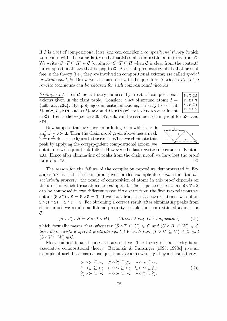
If C is a set of compositional laws, one can consider a compositional theory (whichwe denote with the same latter), that satisfies all compositional axioms from C.We write (S ◦T ⊆ H) ∈ C (or simply S ◦T ⊆ H when C is clear from the context)for compositional laws that belong to C. As usual, predicate symbols that are notfree in the theory (i.e., they are involved in compositional axioms) are called specialpredicate symbols. Below we are concerned with the question: to which extend therewrite techniques can be adopted for such compositional theories?

S ◦ T⊆S

T ◦ S⊆T

S ◦ S⊆T

T ◦ T⊆S

Example 5.2. Let C be a theory induced by a set of compositionalaxioms given in the right table. Consider a set of ground atoms I ={aSb, bTc, cSd}. By applying compositional axioms, it is easy to see thatI C� aSc, I C� bTd, and so I C� aSd and I C� aTd (where C� denotes entailmentin C). Hence the sequence aSb, bTc, cSd can be seen as a chain proof for aSd andaTd.

a

b

c

dS ��?

????

??T

??�������

S

��???

????

S //

T //______

Now suppose that we have an ordering � in which a � b

and c � b � d. Then the chain proof given above has a peakb

T⇐ c

S⇒ d: see the figure to the right. When we eliminate this

peak by applying the correspondent compositional axiom, weobtain a rewrite proof a

S⇒ b

T⇒ d. However, the last rewrite rule entails only atom

aSd. Hence after eliminating of peaks from the chain proof, we have lost the prooffor atom aTd. 33

The reason for the failure of the completion procedure demonstrated in Ex-ample 5.2, is that the chain proof given in this example does not admit the as-sociativity property : the result of composition of atoms in this proof depends onthe order in which these atoms are composed. The sequence of relations S ◦ T ◦ Scan be composed in two different ways: if we start from the first two relations weobtain (S ◦ T) ◦ S = S ◦ S = T, if we start from the last two relations, we obtainS ◦ (T ◦ S) = S ◦ T = S. For obtaining a correct result after eliminating peaks fromchain proofs we require additional property to hold for compositional axioms forC:

(S ◦ T ) ◦ H = S ◦ (T ◦ H) (Associativity Of Composition) (24)

which formally means that whenever (S ◦ T ⊆ U) ∈ C and (U ◦ H ⊆ W ) ∈ Cthen there exists a special predicate symbol V such that (T ◦ H ⊆ V ) ∈ C and(S ◦ V ⊆ W ) ∈ C.

Most compositional theories are associative. The theory of transitivity is anassociative compositional theory. Bachmair & Ganzinger [1995, 1998b] give anexample of useful associative compositional axioms which go beyond transitivity:

� ◦ � ⊆ �; % ◦ % ⊆ %; ∼ ◦ ∼ ⊆ ∼;� ◦ % ⊆ �; � ◦ ∼ ⊆ �; % ◦ ∼ ⊆ %;% ◦ � ⊆ �; ∼ ◦ � ⊆ �; ∼ ◦ % ⊆ %.

(25)

78

For the particular axioms above it is especially easy to check the associativityproperty. Let � be a precedence on special predicate symbols such that � �% � ∼. Then the compositional axioms above can be characterised as follows:

Definition 5.3. Given a precedence � on special predicate symbols, we say that acompositional theory C is induced by � if C = {S◦T ⊆ H | H = max�(S, T )}. 33

All compositional axioms in (25) are induced by the precedence � given above.Every compositional theory that is induced by a precedence �, is evidently asso-ciative, and composition of several special relations can be computed as follows:

S1 ◦ · · · ◦ Sn ⊆ S iff S = max�(S1,.., Sn).

Bachmair & Ganzinger [1998b] have restricted the class of allowed composi-tional axioms to those induced by a total precedence on special predicates. Themodel construction and redundancy elimination will work if one imposes a weakerrestrictions on compositional axioms:

Definition 5.4. We say that a set C of compositional axioms is compatible witha precedence � on special predicates if (S ◦ T ⊆ H) ∈ C implies that S ≥≥ H orT ≥≥ H. 33

However, in this report we do not impose any of these restrictions, since thereare many interesting compositional theories that do not enjoy this property, likethe one given in the example below. Unfortunately, this will require certain mod-ification of standard redundancy for the chaining calculus.

Example 5.5. Consider a theory consisting of special binary predicate symbols Pi

for every natural i with 0 ≤ i < p which admit the following compositional axioms:

Pn ◦ Pm ⊆ P(n+m mod p) (26)

for every n and m with 0 ≤ n < p and 0 ≤ m < p. It is easy to check that thiscompositional theory is associative. Indeed, Pn1

◦ · · · ◦ Pnk⊆ P(n1+···+nk mod p) does

not depend on the order in which these compositional axioms are applied.However, if p > 1, then there is no total precedence � on special predicate

symbols that is compatible with all compositional axioms. Indeed, assume that� is such a precedence and Pm is the maximal special predicate symbol w.r.t.to this precedence. Then P(m−1 mod p) ◦ P(m+1 mod p) ⊆ Pm, hence it is not possiblethat P(m−1 mod p) ≥≥ Pm or P(m+1 mod p) ≥≥ Pm unless either (m − 1 = m mod p), or(m + 1 = m mod p), which is only possible when p = 1. 33

The ordered chaining calculus for compositional binary relations OC�Sel

is for-mulated in System 11. In all inference rules we assume that S, T and H are special

79

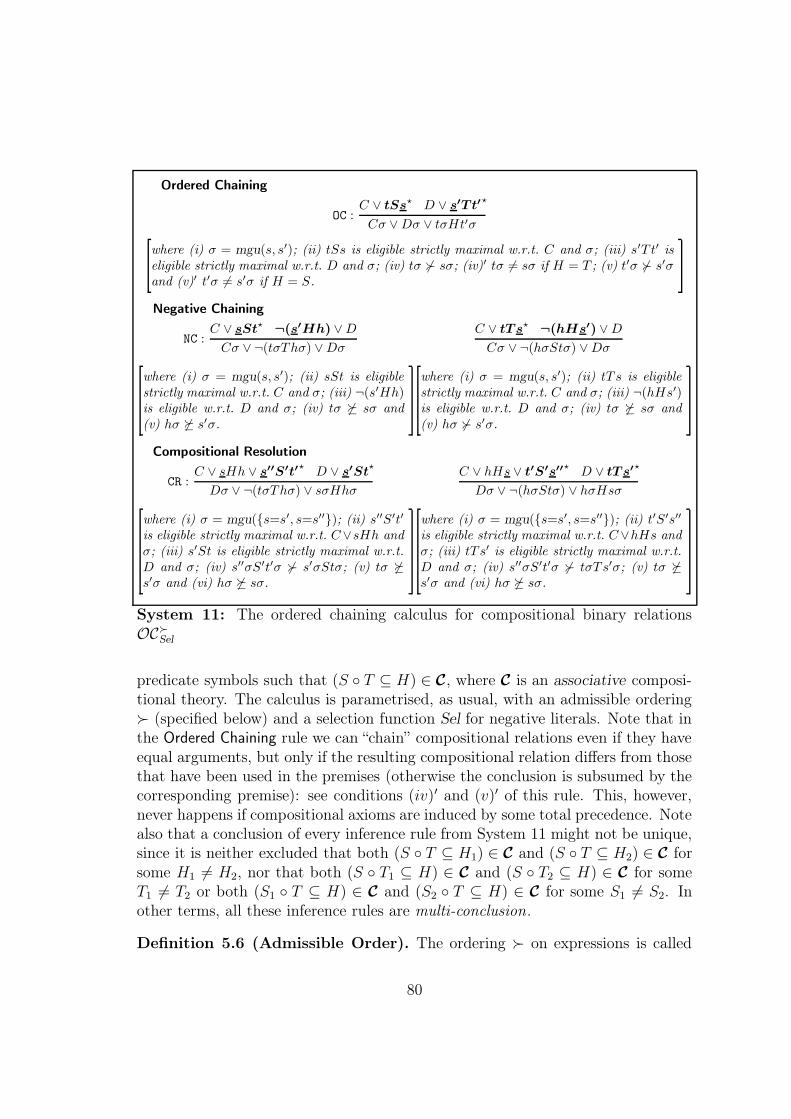
Ordered Chaining

OC :C ∨ tSs? D ∨ s′Tt′?

Cσ ∨ Dσ ∨ tσHt′σ

where (i) σ = mgu(s, s′); (ii) tSs is eligible strictly maximal w.r.t. C and σ; (iii) s′T t′ iseligible strictly maximal w.r.t. D and σ; (iv) tσ 6� sσ; (iv)′ tσ 6= sσ if H = T ; (v) t′σ 6� s′σand (v)′ t′σ 6= s′σ if H = S.

Negative Chaining

NC :C ∨ sSt? ¬(s′Hh) ∨ D

Cσ ∨ ¬(tσThσ) ∨ Dσ

C ∨ tTs? ¬(hHs′) ∨ D

Cσ ∨ ¬(hσStσ) ∨ Dσ

where (i) σ = mgu(s, s′); (ii) sSt is eligiblestrictly maximal w.r.t. C and σ; (iii) ¬(s′Hh)is eligible w.r.t. D and σ; (iv) tσ 6� sσ and(v) hσ 6� s′σ.

where (i) σ = mgu(s, s′); (ii) tT s is eligiblestrictly maximal w.r.t. C and σ; (iii) ¬(hHs′)is eligible w.r.t. D and σ; (iv) tσ 6� sσ and(v) hσ 6� s′σ.

Compositional Resolution

CR :C ∨ sHh ∨ s′′S′t′? D ∨ s′St

?

Dσ ∨ ¬(tσThσ) ∨ sσHhσ

C ∨ hHs ∨ t′S′s′′? D ∨ tTs′?

Dσ ∨ ¬(hσStσ) ∨ hσHsσ

where (i) σ = mgu({s=s′, s=s′′}); (ii) s′′S′t′

is eligible strictly maximal w.r.t. C∨sHh andσ; (iii) s′St is eligible strictly maximal w.r.t.D and σ; (iv) s′′σS′t′σ 6� s′σStσ; (v) tσ 6�s′σ and (vi) hσ 6� sσ.

where (i) σ = mgu({s=s′, s=s′′}); (ii) t′S′s′′

is eligible strictly maximal w.r.t. C∨hHs andσ; (iii) tT s′ is eligible strictly maximal w.r.t.D and σ; (iv) s′′σS′t′σ 6� tσTs′σ; (v) tσ 6�s′σ and (vi) hσ 6� sσ.

System 11: The ordered chaining calculus for compositional binary relationsOC�

Sel

predicate symbols such that (S ◦ T ⊆ H) ∈ C, where C is an associative composi-tional theory. The calculus is parametrised, as usual, with an admissible ordering� (specified below) and a selection function Sel for negative literals. Note that inthe Ordered Chaining rule we can “chain” compositional relations even if they haveequal arguments, but only if the resulting compositional relation differs from thosethat have been used in the premises (otherwise the conclusion is subsumed by thecorresponding premise): see conditions (iv)′ and (v)′ of this rule. This, however,never happens if compositional axioms are induced by some total precedence. Notealso that a conclusion of every inference rule from System 11 might not be unique,since it is neither excluded that both (S ◦ T ⊆ H1) ∈ C and (S ◦ T ⊆ H2) ∈ C forsome H1 6= H2, nor that both (S ◦ T1 ⊆ H) ∈ C and (S ◦ T2 ⊆ H) ∈ C for someT1 6= T2 or both (S1 ◦ T ⊆ H) ∈ C and (S2 ◦ T ⊆ H) ∈ C for some S1 6= S2. Inother terms, all these inference rules are multi-conclusion.

Definition 5.6 (Admissible Order). The ordering � on expressions is called

80

admissible for chaining if � is admissible for resolution (see Definition 3.34) andadditional:

(T) � is total on ground terms,

and for every compositional axiom S ◦T ⊆ H and terms s � t, s � h, the followinghold:

(C1) ¬(sHh) � (sSt); ¬(hHs) � (tT s); ¬(sHs) � (tT s);(C2) ¬(sHh) � ¬(tTh); ¬(hHs) � ¬(hSt); ¬(sHs) � ¬(sSt);(C3) (sSt) � ¬(tTh); (tT s) � ¬(hSt); (sHs) � (sSt) 33

Conditions (C1) and (C2) are needed to ensure monotonicity of the NegativeChaining rule and condition (C3) guarantees monotonicity of the CompositionalResolution rule:

Lemma 5.7 (Monotonicity for OC�Sel

). All rules except the Ordered Chaining

rule from OC�Sel

are monotone for ground clauses w.r.t. every admissible ordering.

Proof. (1) Negative Chaining:We show that the conclusion of this rule is always smaller than its right premise:

(1.a) NC : C ∨sSt?, ¬(sHh)∨D ` C ∨¬(tTh)∨D (Negative Chaining, left):By conditions (iv) and (v) of this rule we must have s � t and s � h (we usetotality condition (T) for ordering � here). Since S ◦ T ⊆ H, by conditions (C1)and (C2) of admissible orderings (see Definition 5.8), we have ¬(sHh) � (sSt)and ¬(sHh) � ¬(tTh). By condition (ii) of the rule we have (sSt) � C. Hence¬(sHh) � C. An so, (¬(sHh) ∨ D) � (C ∨ ¬(tTh) ∨ D).

(1.b) NC : C∨tT s?, ¬(hHs)∨D ` C∨¬(hSt)∨D (Negative Chaining, right):By condition (v) of this rule we must have s � h. If s � h, then the situation isfully symmetric to the left version of this rule. If s = h, then we should use thelast properties from conditions (C1) and (C2): ¬(hHs) = ¬(sHs) � (tT s) and¬(hHs) = ¬(sHs) � ¬(sSt). Again, since (tT s) � C by condition (ii) of the rule,we obtain (¬(hHs) ∨ D) � (C ∨ ¬(hSt) ∨ D).

(2) Compositional Resolution:We show that the conclusion of this rule is smaller that its right premise:

(2.a) CR : C ∨ sHh ∨ sS′t′?, D ∨ sSt? ` D ∨ ¬(tTh) ∨ sHh (CompositionalResolution, left):By conditions (iv) and (ii) of this rule, we have (sSt) � (sS ′t) � (sHh). Addition-ally, by condition (C3) of admissible orderings, we have (sSt) � ¬(tTh). Hence(D ∨ sSt) � (D ∨ ¬(tTh) ∨ sHh).

(2.b) CR : C ∨ hHs ∨ t′S′s?, D ∨ tT s? ` D ∨ ¬(hSt) ∨ hHs (Compositional

Resolution, right):This case is completely symmetric to case (2.a). 22

81

Unfortunately the Ordered Chaining rule might not be monotone if the underly-ing compositional axioms are not compatible with any total precedence on specialpredicate symbols (see Definition 5.4 and Example 5.5). Indeed, for every ordering� that is monotone for the Ordered Chaining rule, one can define such a prece-dence � by setting S � T iff cSc � cT c, where c is some fixed constant. Thenmonotonicity of the Ordered Chaining rule would imply that max�(cSc, cT c) � cHcfor every compositional axiom S ◦ T ⊆ H, hence S ≥≥ H or T ≥≥ H and so allcompositional axiom would have been admissible with �.

5.3 The Subterm Chaining Calculus

It is possible to combine the chaining calculus and the superposition calculus tohandle compositional theories with equality. One could simply use the OrderedParamodulation rule to perform paramodulation into non-equational literals (in-cluding all special non-equational literals) as before. However it is possible touse the advantage of compositional theory and perform paramodulation inferencesonly into the largest argument of special literals. Essentially, we treat the equalitypredicate ' as a part of a compositional theory. We assume that every composi-tional theory C contains all axioms ' ◦ S ⊆ S and S ◦ ' ⊆ S for every specialpredicate symbol S. However we do not allow the equational predicate to be theresult of composition of non-equational predicates, i.e., S ◦ T ⊆ ' implies S = 'and T = '. This is done to avoid problems with monotonicity.

Applying these modifications, we obtain a so-called subterm chaining calculusthat is an extension of the ordered chaining calculus from System 11 with infer-ence rules given in System 12, where now equality can be used as a compositionalpredicate symbol. Note that the Positive Superposition and the Negative Superposi-tion rules are instances of the Ordered Subterm Chaining and the Negative SubtermChaining rules respectively, when S = ' (in the left variants). The right variantsof these rules are not needed for equational literals, since we treat equality sym-metrically. The Equality Factoring rule is simulated by a self-application of theCompositional Resolution rule for equational atoms.

Definition 5.8 (Admissible Order). The ordering � on expressions is calledadmissible (for subterm chaining) if � is admissible for chaining (see Definition 5.8)and superposition (see Definition 4.15). 33

Lemma 5.9 (Monotonicity for SC�Sel

). All rules except the Ordered Chaining

rule from SC�Sel are monotone for ground clauses w.r.t. every admissible ordering.

Proof. Monotonicity of the Negative Chaining, Compositional Resolution, ReflexivityResolution and Equality Factoring rules has been already shown (see Lemma 5.7and Lemma 4.16). The remaining rules Ordered Subterm Chaining and Negative

82

Ordered Paramodulation Reflexivity Resolution

OP :C ∨ s ' t? D ∨ L[s′]

Cσ ∨ Dσ ∨ L[t]σRR :

C ∨ s 6' s′

Cσ

where (i) σ = mgu(s, s′); (ii) s ' t is eligiblestrictly maximal w.r.t. C and σ; (iii) L[s′]is eligible (strictly maximal if positive) w.r.t.D and σ; (iv) L[s′] is a non-special literal;(v) tσ 6� sσ and (vi) s′ is not a variable.

where (i) σ = mgu(s, s′) and (ii) s 6' s′ iseligible w.r.t. C and σ.

Ordered Subterm Chaining

OSC :C ∨ s ' t? r[s′]Sh

?∨ D

Cσ ∨ r[t]σShσ ∨ Dσ

C ∨ s ' t? hSr[s′]?∨ D

Cσ ∨ hσSr[t]σ ∨ Dσ

where (i) σ = mgu(s, s′); (ii) s ' t is eligiblestrictly maximal w.r.t. C and σ; (iii) rShis eligible strictly maximal w.r.t. D and σ;(iv) (sσ ' tσ) 6� (rσShσ); (v) tσ 6� sσ;(vi) hσ 6� rσ and (vii) s′ is not a variable.

where (i) σ = mgu(s, s′); (ii) s ' t is eligiblestrictly maximal w.r.t. C and σ; (iii) hSris eligible strictly maximal w.r.t. D and σ;(iv) (sσ ' tσ) 6� (hσSrσ); (v) tσ 6� sσ;(vi) hσ 6� rσ; (vi)′ S 6= ', and (vii) s′ isnot a variable.

Negative Subterm Chaining

NSC :C ∨ s ' t? ¬(r[s′]Sh) ∨ D

Cσ ∨ ¬(r[t]σShσ) ∨ Dσ

C ∨ s ' t? ¬(hSr[s′]) ∨ D

Cσ ∨ ¬(hσSr[t]σ) ∨ Dσ

where (i) σ = mgu(s, s′); (ii) s ' t is eligiblestrictly maximal w.r.t. C and σ; (iii) ¬(rSh)is eligible w.r.t. D and σ; (iv) tσ 6� sσ;(v) hσ 6� rσ and (vi) s′ is not a variable.

where (i) σ = mgu(s, s′); (ii) s ' t is eligiblestrictly maximal w.r.t. C and σ; (iii) ¬(hSr)is eligible w.r.t. D and σ; (iv) tσ 6� sσ;(v) hσ 6� rσ; (v)′ S 6= ', and (vi) s′ is not avariable.

System 12: The subterm chaining calculus SC�Sel

Subterm Chaining are monotone since they are restricted versions of the OrderedParamodulation rule. 22

Admissible orderings for the chaining calculi can be obtained by taking any totalreduction ordering � on ground terms and non-special atoms (say, KBO or LPO)and associating with every ground literal L = (E1 S E2) (or L = ¬(E1 S E2))14 acomplexity measure:

c(L) := ( max(L) , 1−pol(L) , min(L) , S(L) , o(L) ) (27)

where max(L) and min(L) are respectively the maximal and the minimal expres-sions from {E1, E2}; pol(L) is the polarity of the literal, (recall, that pol(L) = 1

14We use equational representation for non-special literals as described in subsection 4.1

83

if L is positive and pol(L) = 0 if L is negative, see p. 7); S(L) = S is the specialpredicate symbol of L (if L is non-special literal then we have S(L) := ') and o(L)is the orientation of L: o(L) = 1 if S is non-symmetric and E1 � E2, and o(L) = 0otherwise. Now, the literals are compared according to this vector representation,i.e., by the lexicographic combination (�, >,�,�, >) of orderings (recall the def-inition and properties from p. 20), where � is an ordering on ground terms andnon-special expressions, > is the standard ordering on natural numbers and � isa precedence on special predicate symbols. It is relatively straightforward to verifyall conditions of admissible orderings for the lifting of the ordering defined by thiscomplexity measure.

Note 5.10. In [Bachmair & Ganzinger, 1998b] the class of admissible orders �has been restricted to those induced by a complexity measure similar to (27) (inthis paper these orderings are called strongly admissible). In this report we haveanalysed the completeness proof and formulated more general conditions (C1) –(C3) for admissible orderings. This will allow us to tailor specific orderings fordeciding certain fragments of first-order logic over compositional theories, whichwould not be possible within the class of strongly admissible orderings. 33

5.4 Refutational Completeness

In this section we give a formal proof of refutational completeness for the subtermchaining calculus SC�

Selwhich is the most general chaining calculus from those

we have described. The completeness proof goes as usual, by model constructionwhich associates with each clause set N a candidate model IN⇓ induced by a setof atoms IN , which we view as a labelled rewrite system.

Let I be a set of ground atoms. A (labelled) rewrite relation induced by a setof atoms I is defined by E1

S⇒I E2 (E1

S⇐I E2, E1

S⇔I E2) if (i) E1

S⇒E2 ∈ I (resp.

E1S⇐E2 ∈ I, E1

S⇔E2 ∈ I) or (ii) S = ', E1 = E1[E

′1] and E2 = E2[E

′2] for some

(E ′1 ⇒E ′

2) ∈ I. In other words, a rewrite relation induced by I is a minimal set oflabelled rewrite rules that contains I and monotone w.r.t. equality.

Definition 5.11 (Rewrite Proofs). An atom A := (E S E ′) has a rewriteproof in I (in symbols: E ⇓S

I E ′), if there exists a sequence of expressionsE = E0, E1,.., Ek, Ek+1,.., En = E ′ for 0 ≤ k ≤ n, and a sequence of special predi-cate symbols S1, S2,.., Sn such that: (i) S1 ◦ S2 ◦ · · · ◦ Sn ⊆ S; (ii) Ei−1

Si⇒I Ei for1 ≤ i ≤ k − 1; (iii) Ei−1

Si⇐I Ei for k + 1 ≤ i ≤ n and (iv)15 either Ek−1Sk⇒I Ek or

Ek−1Sk⇔I Ek (see the left part of Figure 18). 33

15This condition is not needed if k = 0

84

Figure 18 Rewrite and non-rewrite proofs for ordered chainingvalleys: elementary non-valleys:

orE0

S︷ ︷S1⇒ E1 · · ·

Sk-1⇒ Ek−1Sk⇒ Ek

Sk+1

⇐ · · ·Sn⇐ En

E0S1⇒ E1 · · ·

Sk-1⇒ Ek−1Sk⇔ Ek

Sk+1

⇐ · · ·Sn⇐ En

E0S1⇐ E1

S2⇒ E2 (peak)

E0S1⇔ E1

S2⇒ E2, E0S1⇐ E1

S2⇔ E2 (plateau)

E0S1⇔ E1

S2⇔ E2 (plane)

In other words, a rewrite proof is a chain consisting of let-to-right rewritesteps followed by at most one two-way rewrite step and a sequence of right-to-leftrewrite steps. These rewrite proofs are called valleys in [Bachmair & Ganzinger,1998b]. The elementary non-valley chains of length 2 can be classified as follows:(i) E0

S1⇐E1S2⇒E2 is a peak ; (ii) E0

S1⇔E1S2⇒E2 or E0

S1⇐E1S2⇔ E2 is a plateau and

(iii) E0S1⇔E1

S2⇔ E2 is a plain. In all these chains it must be that E1 � E0 andE1 � E2. A valley can be seen as a chain that do not contain any peaks, plateausor plains.

A (rewrite) model I⇓ induced by a set of atoms (= labelled rewrite rules) I isdefined by I⇓�A = (E1 S E2) iff A has a rewrite proof in I. Given an expressionE, let IE denotes the set of atoms from I whose non-special expressions are notgreater than E: IE := {(E0 S1 E2) ∈ I | E0 � E, E1 � E}. Then the followingproperty can be shown:

Lemma 5.12 (Properties of Rewrite Proofs). Let I be a set of atoms and A bean atom whose maximal non-special expression is E. Then I⇓� A iff IE⇓�Aiff I(¬A)⇓�A.

Proof. Every rewrite proof in IE or I(¬A) is also a rewrite proof in I. Hencefrom IE⇓�A or I(¬A)⇓� A it follows that I⇓� A. To prove “only if” parts ofthis lemma, suppose the atom A = (E S E ′) has a rewrite proof P := (E =E0 S1 E1 · · · Sn En = E ′). W.l.o.g., assume that E � E ′ (the remaining case isconsidered symmetrically). It follows from the definition of a rewrite proof thatevery expression Ei with 0 ≤ i ≤ n involved in P , is not greater than E. HenceIE⇓� A.

It remains to show that I(¬A) � A as well. For this we need to use the condi-tions of admissible ordering from Definition 5.6. We demonstrate that every atomEi−1 Si Ei from P , is smaller than ¬A. If both Ei−1 and Ei are smaller then E =E0, then ¬A = ¬(E0 S En) � (E0 S ′

i Ei), where S1◦. . .◦Si ⊆ S ′i (by condition (C1)

of admissible orderings). And finally, (E0 S ′i Ei) � ¬(Ei−1 Si Ei) � (Ei−1 Si Ei)

(by conditions (C3) and (R1) of admissible orderings). If either Ei−1 or Ei is equalto E = E0, then Ei−1 Si Ei is either the first or the last step in P . Hence, thefollowing cases can be distinguished: (a) i = 1 and E = E0 = Ei−1 � Ei 6= En, or(b) i = n and E = E0 6= Ei−1 ≺ Ei = En, or (c) i = n = 1, i.e., A = (Ei−1 Si−1 Ei).In case (a), we have ¬A � (Ei−1 Si−1 Ei) by condition (C1) of admissible ordering.

85

Case (b) is symmetric to case (a). In case (c), ¬A � (Ei−1 Si−1 Ei) by condition(R1) of admissible ordering. 22

It is not always true that a rewrite model induced by a set of atoms admitscompositional and/or equational axioms. This is however true if the set of atomsI is complete in the following sense:

Definition 5.13 (Canonical Rewrite System). We say that a plateau, peakor a plain E0 S1 E1 S2 E2 commutes in I if S1 ◦S2 ⊆ S implies that E0 S E2 has arewrite proof in I. A rewrite system I is canonical (for chaining) if every plateau,peak or a plain in I commutes. 33

Below we establish an analog of Critical Pair Lemma for labelled rewrite sys-tems:

Lemma 5.14 (Canonical Proofs). Let I be a canonical rewrite system for or-dered chaining and A be an atom. Then I T� A iff I⇓�A.

Proof. The “if” part of this lemma is trivial, since every rewrite proof in I is achain in I. In order to show the remaining part of the lemma, let P := (E0 S1

E1 S2 E2 · · · Sn En) be a chain for A = (E0 S En) based on I with S1◦· · ·◦Sn ⊆ S.We show by induction on multiset {E0, E1,.., En}m

(w.r.t. the multiset extensionof the ordering � on expressions) that I⇓� A.

Suppose the chain P is not a rewrite proof. Then there should be a peak,a plateau or a plain Ei−1 Si Ei Si+1 Ei+1 in P , i.e., with Ei � Ei−1 and Ei �Ei+1. Since I is canonical, then I⇓� Ei−1 S ′

i+1 Ei+1, where Si ◦ Si+1 ⊆ S ′i+1,

i.e., there is a valley Ei−1 S1i E1

i S2i E2

i · · · Ski Ei+1 with S1

i ◦ S2i ◦ · · ·Sk

i ⊆ S ′i+1

based on I. Note, that in particular Ei � Eji for all j with 1 ≤ j < k, and so,

{Ei−1, Ei, Ei+1}m� {Ei−1, E

1i ,.., E

k−1i , Ei+1}m

. Hence, we found a new chain for Awith a smaller complexity. By induction hypothesis, we obtain that I⇓�A. 22

Definition 5.15 (Candidate Models, Productive Clauses). Let N ⊆ Cl0Σand C ∈ Cl0

Σ. The candidate models IN⇓ for N , IC⇓ for NC and IC⇓ for NC are

induced respectively by the sets IN , IC and IC that are defined as follows:IN :=

⋃C∈N IC ; IC =

⋃C′∈NC

IC′

, and IC := IC ∪ ∆C, where ∆C := {A} if:

(i) IC⇓2 C;

(ii) C = (C ′ ∨ A) where A is an eligible maximal atom w.r.t. C ′, and

(iii) for every C1 = (C ′1 ∨A1) ∈ NC with ∆C1 = {A1}, we have (IC ∪ {A})⇓2 C ′

1.

If there is no atom A satisfying conditions (i) – (iii), we assign ∆C = {}. If∆C 6= {}, we call clause C productive w.r.t. N and say that C produces ∆C. 33

86

Lemma 5.16 (Properties of Candidate Models). Let the candidate modelsand productive clauses for a set N of ground clauses be defined like in Defini-tion 5.15. Then for every C ∈ N , (i) IC⇓� C implies that IN⇓� C, and (ii) ifC = C ′ ∨ A? is a productive clause, then IN⇓2 C ′.

Proof. (i) In order to show the first property, assume that IC⇓� C, but IN⇓2 C.This is only possible if for some atom B = (E1 S E2) occurring negatively in C,we have IC⇓2 B but IN⇓� B. Then by Lemma 5.12, I(¬B)⇓�B, which is notpossible since ¬B � C.

Part (ii) of this lemma is guaranteed by the case (iii) of the definition forproductive clauses (see Definition 5.15). 22

Lemma 5.17 (Counterexample-Reduction Lemma). Let N be a set of groundclauses which is saturated w.r.t. SC�

Sel. Then for every clause D ∈ N with IN⇓2 D 6=

�, there exists a clause D1 ∈ N such that D1 ≺ D and IN⇓2 D1.

Proof. If D is a counterexample for IN⇓, i.e., IN⇓2 D, then ID⇓ = ID⇓2 D (herewe use Lemma 5.16 (i)). By Lemma 5.16 (ii), D cannot be a productive clause,so Definition 5.15 leaves us only the following possibilities:

(1) D = (D′ ∨ ¬A), where ¬A is an eligible literal in D, and ID⇓� A =(E1 H E2) for some special predicate symbol H. For definiteness, assume thatE1 � E2 (the remaining case E2 � E1 is considered symmetrically). Then either(1.1) H = ' and E1 = E2 = s for some ground term s, or (1.2) A = (P ' T)

is a non-special atom and P is reducible by some rewrite rule (E ′1 ⇒E ′

2) ∈ IC ,16

or (1.3) E1 = s, E2 = h and the first step in the rewrite proof of A = (sHh) iss

S⇒ t for some S 6= ' and a ground term t ≺ s, or (1.4) E1 = r[s], E2 = h and

the first step in the rewrite proof of A = (r[s]Hh) is done by (s⇒ t) ∈ ID. Thecases (1.1) and (1.2) are identical to those considered for the paramodulation andsuperposition calculi. The principally new cases for the chaining calculus are (1.3)and (1.4).

N Clauses C ∆C

D D′ ∨ ¬(sHh) −g

D1 C ′ ∨ D′ ∨ ¬(tTh) ?

C C ′ ∨ sSt? sS⇒ t

In case (1.3) the rewrite rule sS⇒ t must be pro-

duced by some productive clause C = (C ′∨sSt?) ≺ D.Moreover, there exists a special predicate symbol Tsuch that S ◦T ⊆ H and IN⇓�(tTh). Then a NegativeChaining inference with the conclusion NC[C, D]: D1 =(C ′ ∨D′ ∨¬(tTh)) ∈ N is possible which is a smaller clause than D. D1 is a coun-terexample for IN⇓, since IN⇓2 D′, IN⇓�(tTh) and IN⇓2 C ′ by Lemma 5.16 (ii).

16Note that no labeled rewrite rule can be used in a rewrite proof for A, since P is not a term

87

N Clauses C ∆C

D D′ ∨ ¬(r[s]Hh) −g

D1 C ′ ∨ D′ ∨ ¬(r[t]Hh) ?

C C ′ ∨ s ' t? s⇒ t

In case (1.4) the rewrite rule s⇒ t is producedby some productive clause C = (C ′ ∨ s ' t?). Thenthe Negative Subterm Chaining rule can be applied toC and D which produces a clause NSC[C, D]: D1 =(C ′ ∨ D′ ∨ ¬(r[t]Hh)) ∈ N which is a smaller coun-terexample for IN⇓ than D.

N Clauses C ∆C

D D′ ∨ (E1 S E2)︸ ︸A

−

g

C C ′′ ∨

B︷ ︷(E′

1 H E′2) ∨ A1

? A1

(2) D = (D′∨A), where A = (E1 S E2) is an el-igible maximal literal in D, but D is not productivebecause condition (iii) from Definition 5.15 is vio-lated. In this case, there exists a productive clauseC = (C ′ ∨ A1

?) � D, such that (ID ∪ A)⇓� C ′,i.e., C ′ = (C ′′ ∨ B) where (ID ∪ A)⇓� B = (E ′

1 H E ′2). Assume that E1 � E2

(the case E2 � E1 is considered symmetrically). Then E1 � E ′1 and E1 � E ′

2,since otherwise for E ′ := max{E ′

1, E′2}, we have IN⇓� IE′

⇓ = (ID ∪A)E′

⇓�B (byLemma 5.12) which is not possible by Lemma 5.16 (ii). Since atom A is used inthe rewrite proof of B, then E1 = E ′

1 and either (2.1) it is a one-step rewrite proof,i.e., A = B, or (2.2) A 6= B and E1 � E2: see the definition of rewrite proofs(Definition 5.11). In case (2.1) A � A1 � B = A hence C = D, A1 = B and thecounterexample can be reduced using the Ordered Factoring rule.

N Clauses C ∆C

D D′ ∨ sSt? −g

D1 D′ ∨ ¬(tTh) ∨ sHh ?C C ′ ∨ sHh ∨ sS′t′? A

In case (2.2), A and B must be special atoms: A =(sSt) and B = (sHh) for some ground terms s � tand s � h. The case s = h is not possible becauseotherwise by the last property from condition (C3) ofadmissible orderings (see Definition 5.8), we have B =

(sHs) � (sSt) = A. Since (IN ∪ {sS⇒ t})⇓� sHh then IN⇓� tTh for some special

predicate symbol T such that S ◦ T ⊆ H. Then the conclusion CR[C, D]: D1 =(D′∨¬(tTh)∨sHh) a Compositional Resolution inference, which is a smaller clausethan D1, must belong to N . Since IN⇓2 D′, IN⇓�(tTh) and IN⇓2 sHh (the lastis by Lemma 5.16 (ii) applied to C), we have obtained a smaller counterexamplethan D. 22

Remark 5.18. It is possible to dramatically restrict the Compositional Resolutionrule when the maximal literal s′′S ′t′ in the left premise is equality. We show that inthe correspondent case of Counterexample-Reduction Lemma (Lemma 5.17, case(2.2)) a counterexample can be reduced using the Ordered Subterm Chaining orthe following extension of the Equality Factoring rule for other special predicatesymbols: see Figure 19.

88

Figure 19 An extension of the Equality Factoring rule for compositional theories

Equality Factoring

EF :C ∨ s′Hh ∨ s ' t?

Cσ ∨ ¬(tσHhσ) ∨ s′σHhσ

C ∨ hHs′ ∨ s ' t?

Cσ ∨ ¬(hσHtσ) ∨ hσHs′σ

where (i) σ = mgu(s, s′); (ii) s ' t is eligiblestrictly maximal w.r.t. C ∨ s′Hh and σ, and(iii) tσ 6� sσ.

where (i) σ = mgu(s, s′); (ii) s ' t is eligiblestrictly maximal w.r.t. C ∨ hHs′ and σ, and(iii) tσ 6� sσ.

N Clauses C ∆C

D D′ ∨ sSt? −g

D2 C ′ ∨ sHh ∨ t′St ∨ D′ ?

C C ′ ∨ sHh ∨ s ' t′? s⇒ t′

gD1 C ′ ∨ ¬(t′Hh) ∨ sHh ?

Indeed, if in case (2.2) of Lemma 5.17 S ′ = ' ,then there are only two following cases possible:

Case (a) IN⇓�(t′St). Since IN⇓� tTh, thenIN⇓�(t′Hh) and the conclusion EF[C]: D1 = (C ′∨¬(t′Hh) ∨ sHh) ∈ N of an Equality Factoring in-ference from C is a smaller counterexample thanD.

Case (b) IN⇓2(t′St). Then the conclusion OSC[C, D]: D2 = (C ′ ∨ sHh∨ t′St∨D′) ∈ N of an Ordered Subterm Chaining inference from C and D is a smallercounterexample than D. 33

Note 5.19. In the original completeness proofs for ordered chaining calculi, Bach-mair & Ganzinger [1995, 1998b] used a slightly different model construction. Givena saturated set of clauses N they have showed by induction over a well ordering� that IC⇓� C. So the counterexamples in their sense are those clauses C thatare false in IC⇓ (not in IN⇓ like here). The advantage of the model constructionthat we have presented here is twofold. First, the structure and philosophy of ourproof goes along with the completeness proofs for the ordered resolution and thesuperposition calculi. Second, we clearly separate properties of candidate modelsfor arbitrary clause sets (in Lemma 5.16) from those for saturated sets of clauses(in Lemma 5.17).

Going slightly deeper into details, condition (iii) of productive clauses (see Def-inition 5.15) is missing in [Bachmair & Ganzinger, 1995, 1998b] which clearly givesproblems with the property (ii) from Lemma 5.16. Without this condition, theproperties of productive clauses and counterexample reduction have to be demon-strated together in one inductive proof, which can be carried out only for saturatedclause sets. 33

5.5 Hyper-Inferences

It is possible to define hyper-inferences for the chaining calculi in similar fashion asit has been done for the resolution calculus (see Figure 8 and Figure 9 on p.58). A

89

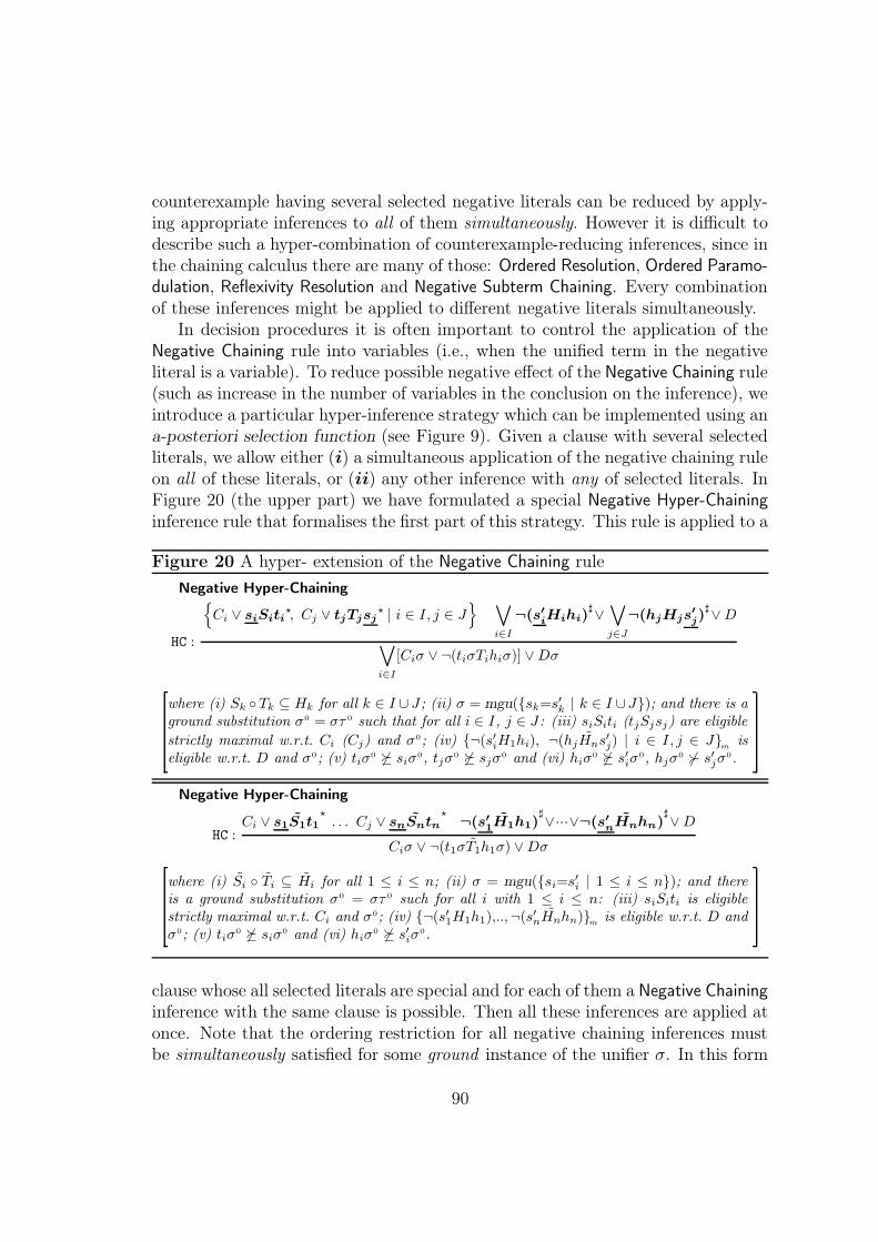
counterexample having several selected negative literals can be reduced by apply-ing appropriate inferences to all of them simultaneously. However it is difficult todescribe such a hyper-combination of counterexample-reducing inferences, since inthe chaining calculus there are many of those: Ordered Resolution, Ordered Paramo-dulation, Reflexivity Resolution and Negative Subterm Chaining. Every combinationof these inferences might be applied to different negative literals simultaneously.

In decision procedures it is often important to control the application of theNegative Chaining rule into variables (i.e., when the unified term in the negativeliteral is a variable). To reduce possible negative effect of the Negative Chaining rule(such as increase in the number of variables in the conclusion on the inference), weintroduce a particular hyper-inference strategy which can be implemented using ana-posteriori selection function (see Figure 9). Given a clause with several selectedliterals, we allow either (i) a simultaneous application of the negative chaining ruleon all of these literals, or (ii) any other inference with any of selected literals. InFigure 20 (the upper part) we have formulated a special Negative Hyper-Chaininginference rule that formalises the first part of this strategy. This rule is applied to a

Figure 20 A hyper- extension of the Negative Chaining rule

Negative Hyper-Chaining

HC :

{Ci ∨ siSiti

?, Cj ∨ tjTjsj? | i ∈ I, j ∈ J

} ∨

i∈I

¬(s′iHihi)

]∨

∨

j∈J

¬(hjHjs′j)

]∨ D

∨

i∈I

[Ciσ ∨ ¬(tiσTihiσ)] ∨ Dσ

where (i) Sk ◦Tk ⊆ Hk for all k ∈ I ∪ J ; (ii) σ = mgu({sk=s′k | k ∈ I ∪ J}); and there is aground substitution σ0 = στ 0 such that for all i ∈ I, j ∈ J : (iii) siSiti (tjSjsj) are eligible

strictly maximal w.r.t. Ci (Cj) and σ0; (iv) {¬(s′iH1hi), ¬(hjHns′j) | i ∈ I, j ∈ J}m

iseligible w.r.t. D and σ0; (v) tiσ

0 6� siσ0, tjσ

0 6� sjσ0 and (vi) hiσ

0 6� s′iσ0, hjσ

0 6� s′jσ0.

Negative Hyper-Chaining

HC :Ci ∨ s1S1t1

?. . . Cj ∨ snSntn

?¬(s′

1H1h1)

]∨···∨¬(s′

nHnhn)]∨ D

Ciσ ∨ ¬(t1σT1h1σ) ∨ Dσ

where (i) Si ◦ Ti ⊆ Hi for all 1 ≤ i ≤ n; (ii) σ = mgu({si=s′i | 1 ≤ i ≤ n}); and thereis a ground substitution σ0 = στ 0 such for all i with 1 ≤ i ≤ n: (iii) siSiti is eligiblestrictly maximal w.r.t. Ci and σ0; (iv) {¬(s′1H1h1),..,¬(s′nHnhn)}

mis eligible w.r.t. D and

σ0; (v) tiσ0 6� siσ

0 and (vi) hiσ0 6� s′iσ

0.

clause whose all selected literals are special and for each of them a Negative Chaininginference with the same clause is possible. Then all these inferences are applied atonce. Note that the ordering restriction for all negative chaining inferences mustbe simultaneously satisfied for some ground instance of the unifier σ. In this form

90

the rule is more restrictive than if the ordering restrictions are verified separatelyfor σ, as is usually done (recall the discussion from Example 3.35). This helps tofilter-out many unnecessary chaining inferences:

Example 5.20. Consider a clause D := (¬xxTTyy ∨ ¬yyTTxx), where T is a transitivepredicate symbol. Both negative literals in this clause are maximal, since theydiffer only by permutation of variables. Hence it is possible to apply the OrderedChaining rule to both of them, e.g., with a clause C := f(x)Tx. However theNegative Hyper-Chaining rule with (two copies of) C cannot be applied to bothliterals of D simultaneously, since condition (vi) of this rule is violated. Indeed,there is no ground substitution σ0 such that yσ0 6� xσ0 and xσ0 6� yσ0. Note, thatthis condition can be possibly satisfied for a non-ground substitution σ. 33

To simplify the exposition and usage of the Negative Hyper-Chaining rule (inparticular the annoying distinction between “left” and “right” arguments of specialpredicate symbols), we introduce additional notation. For every binary predicatesymbol S, we introduce a shortcut S` that denotes the inverse of S, i.e., (xS`t) :=(tSx). According to this notation, every compositional axiom S ◦ T ⊆ H inducesa compositional axiom T ` ◦S` ⊆ H` on inverse relations. Finally, let S stand forS or S`. Using this notation, the Negative Hyper-Chaining can be formulated morecompactly (although with condition (vi) relaxed) in the lower part of Figure 20.

5.6 Redundancy

The standard redundancy criterion based on semantical entailment cannot be di-rectly adapted for the chaining calculus. The problem is caused by the OrderedChaining rule which might be not monotone. Note that monotonicity of thisrule has not been used in our model construction, in particular in the proof ofCounterexample-Reduction Lemma (Lemma 5.17), since this rule may not reducecounterexamples. The sole purpose of this rule is to guarantee that the candidatemodel IN⇓ constructed for a saturated clause set N is a C-model.

To show why the standard redundancy does not work, suppose, that we havea compositional axiom (S ◦ T ⊆ H) ∈ C with H 6= S, H 6= T and tHt � tSt,tHt � tT t for some ground term t. That is, we have a situation when the OrderedChaining inference from clauses tSt and tHt is possible but not monotone. Usingthe standard redundancy criterion based on semantical entailment (w.r.t. a theoryC), it is easy to see that clause C := tHt is redundant w.r.t. an unsatisfiable clauseset N := {tSt, tT t, tHt, ¬(tHt)}, since NC := {tSt, tT t} C� tHt. However, theempty clause could not be derived from N if we delete clause C permanently . Ifwe analyse the model construction given in Counterexample Reduction Lemma(Lemma 5.17), we notice that although NC C� C, this does not suffices to establishthat IC⇓� C, since IC⇓ is not necessarily a C-model. In the particular example

91

above, we cannot delete C, because it is a productive clause that should reducethe minimal counterexample in N .

Let us review the arguments used to justify the standard redundancy criterion.A ground clause C ∈ N might not be considered in the model construction, ifwe know a-priory that either IN⇓2 NC (which is by Lemma 5.16 (i) equivalentto IC⇓2 NC), or IC⇓� C (hence C is not a productive clause and not a coun-terexample). In both cases C may neither be a minimal counterexample nor aproductive clause that reduces the minimal counterexample. To put it simple, aclause C is redundant if IC⇓�NC implies IC⇓� C. However, contrary to paramo-dulation or superposition calculi, the set NC is not necessary saturated under thechaining inference rules even if N is saturated. Hence, IC might not be canonical,and so IC⇓ is might not be a C-model, which means that NC C�C is not sufficientto establish redundancy.

It is possible to characterise redundancy by means of rewrite proofs, similarlyas it is done for instance in [Bachmair & Ganzinger, 1997], by noticing that ev-ery set IC must be closed under monotone Ordered Chaining inferences. However,demonstrating entailment via rewrite proofs is less convenient than by semanticalarguments, therefore we formulate redundancy using a sufficient semantical ap-proximation. Note that in order to establish redundancy for C, it suffices to showthat IC1⇓� NC1 implies IC1⇓� C for some C1 ≺ C. If the last property holdsthen either there exists a counterexample in NC1 , which is smaller than C, or theclause C is not productive, hence C might not be considered. Although IC is notclosed under the Ordered Chaining rule, the set IC1 might be closed. This idea isformalised using the following notion:

Definition 5.21 (Redundancy Ordering). A redundancy ordering for an ad-missible ordering � (for chaining calculi) is a partial ordering �· on ground literalssuch that the following conditions hold:

(CRO1) �· ⊆ �, � ◦ �· ⊆ �, �· ◦ � ⊆ �;(CRO2) S ◦ T ⊆ H, L �· tSs, L �· sTh and s � t, s � h

imply that L �· tHh 33

Using a redundancy ordering we can express a property for inference systemswhich is weaker than monotonicity. An inference π (an inference system S) isweakly monotone w.r.t. �· , if for every ground clause C 0 the set of the clausesthat are ≺· -smaller than C 0, is closed under π (respectively S). Note that if π ismonotone w.r.t. � for ground clauses, then it is weakly monotone w.r.t. �.

Condition (CRO1) from Definition 5.21 expresses that �· is a partial sub-ordering of � which is closed under composition with �. This is needed to insurethat every inference that is monotone w.r.t. � remains weakly monotone w.r.t. �· .Note that if � is well-founded, then �· is also well-founded. Condition (CRO2) isneeded to ensure that the Ordered Chaining rule is weakly monotone w.r.t. �· .

92

Lemma 5.22 (Weak Monotonicity for SC�Sel

). The subterm chaining calculusSC�

Selis weakly monotone w.r.t. every redundancy ordering �· for any admissible

ordering �.

For example, given an admissible ordering � defined by (27), a redundancyordering �· for � can be induced by the following complexity measure on literals:

c(L) := ( max(L) , 1−pol(L) , min(L) ) (28)

It is easy to see that this ordering fulfils both conditions from Definition 5.21 w.r.t.� from (27).

Now, the standard redundancy criterion is defined as usual, but w.r.t. a redun-dancy ordering �· instead of an admissible ordering �:

Definition 5.23 (Standard Redundancy). Given a set of ground clauses N 0,and a ground clause C 0, let N 0

≺·C0 := {C 01 ∈ N 0 | C 0

1 ≺· C 0} be the set of groundclauses from N 0 that are ≺· -smaller than C 0.

A ground clause C 0 is redundant w.r.t. a set of ground clauses N 0, if C 0 followsin C from the set N 0

≺·C0 . A ground inference π0 is redundant w.r.t. N 0 in SC�Sel

′ ifeither π0 /∈ SC�

Sel′ or, otherwise, the conclusion of π0 follows in C from N 0

≺·C0i

forsome premise C 0

i of π0.A (general) clause C is redundant w.r.t. a clause set N if every ground instance

C 0 ∈ {C}gr of C follows in C from N gr. An inference π is redundant w.r.t. N inSC�

Sel, if for every projection Sel′ of Sel from the premises of π, the ground instance

π0 of π is redundant w.r.t. N gr in SC�Sel

′ .We denote this redundancy criterion by R

S �· = (R�·Cl(·), R

S �·Inf (·)). 33

It is easy to show that this notion of redundancy is a redundancy criterionindeed according to Definition 3.20: the proof of this fact is just a repetition of theproof for Lemma 3.21 (for this we only need to use that �· is well founded). Finally,we establish completeness for the subterm chaining calculus with redundancy:

Theorem 5.24 (Completeness of SC�

Selwith Redundancy).

(SC�Sel

, RS �· ) is complete for every selection function Sel, admissible ordering �and every redundancy ordering �· for �.

Proof. Let N be saturated up to redundancy and N gr be the set of ground in-stances of N . We need to consider a situation, when an inference π reducing acounterexample D in N gr is redundant w.r.t. N gr, i.e., the conclusion D1 of π fromNgr follows from clauses N≺·D in theory C. Since the subterm chaining calculusis weakly monotone w.r.t. �· , then N≺·D is saturated under SC�

Sel. By induction

hypothesis, I≺·D⇓ is a C-model for N≺·D and consequently for D1. Thus, I≺·D⇓� D1

which means that D1 is not a counterexample. So redundant inferences might notbe used for reduction of counterexamples. 22

93

6 Clause Normal Form Transformation

Saturation-based theorem provers operate not with first-order formulas but withsets of clauses. To use provers for full first-order logic, it is required to transformformulas into a clause normal form (CNF). It is well-known that the quality of theCNF- transformation has a great impact on efficiency and success of the overalltheorem proving attempt. There are examples, where (naïve) textbook proceduresproduce exponentially large CNF’s in the size of the input first-order formula,which makes them not very useful in practice.

For saturation-based decision procedures the CNF-transformation plays evenmore important rôle, since the transformation has to map a decidable first-orderfragment into a decidable clause class. Thus, essential properties, that contributeto decidability of a particular first-order fragment should be inherited into theirclause representations.

CNF-transformation has been thoroughly studied in literature [for the overviewsee Nonnengart & Weidenbach, 2001; Baaz, Egly & Leitsch, 2001]. The traditionalway of producing CNF’s for decidable first-order fragments consists of three mainsteps. First, a formula is translated into a negation normal form by pushing nega-tion inwards as far as possible. Second, a so-called structural transformation isapplied to a formula, that splits the formula into a conjunction of simple formu-las. In the last step, skolemization is employed that introduces Skolem functionsfor existentially quantified variables. After this step the universal quantifiers aredropped and the result is written in a clause form.

Below we present all these transformations in their general form and later wegive their variants for considered first-order fragments. In our presentation we makea special emphasis on complexity issues of transformations. We estimate a worsttime complexity of transformations and the size of their results. Some materialpresented in this section belongs to a logical folklore (especially transformationprocedures and complexity calculations), therefore it is hard to give any referenceor historical remarks about them. For the same reason, many proofs may seem toosketchy. This section does not aim in giving comprehensive account of techniquesand results about CNF transformation. For those, the reader is forwarded to theoverview articles [Nonnengart & Weidenbach, 2001; Baaz et al., 2001] where manyaspects of doing CNF-transformation in efficient way are presented and furtherlinks to literature are provided.

6.1 Negation Normal Form

A first-order formula (involving conjunction, disjunction and negation as the onlyboolean connectives) is in negation normal form (or shortly NNF) if negationsymbol appears only in front of atoms in this formula. A transformation that puts

94

a first-order formula into NNF is probably the simplest normalization step. Givena first-order formula, one has to distribute negation over other boolean connectivesand quantifiers using the usual de-Morgan’s lows:

¬(A ∧ B) ⇒ ¬A ∨ ¬B¬(A ∨ B) ⇒ ¬A ∧ ¬B

¬¬A ⇒ A¬∀x.A ⇒ ∃x.¬A¬∃x.A ⇒ ∀x.¬A

(29)

Figure 21 Negation normal form transformation for first-order formulas

FO ::= A | F1 ∨ F2 | F1 ∧ F2 | ¬F1 | ∀y.F1 | ∃y.F1.

[F ]nnf := [A]nnf = A |

[F1 ∧ F2]nnf = [F1]

nnf ∧ [F2]nnf |

[F1 ∨ F2]nnf = [F1]

nnf ∨ [F2]nnf |

[¬F1]nnf = [F1]

nnf¬ |

[∀y.F1]nnf = ∀y.[F1]

nnf |

[∃y.F1]nnf = ∃y.[F1]

nnf .

[F ]nnf¬ := [A]nnf = ¬A |

[F1 ∧ F2]nnf¬ = [F1]

nnf¬ ∨ [F2]

nnf¬ |

[F1 ∨ F2]nnf¬ = [F1]

nnf¬ ∧ [F2]

nnf¬ |

[¬F1]nnf¬ = [F1]

nnf |

[∀y.F1]nnf¬ = ∃y.[F1]

nnf¬ |

[∃y.F1]nnf¬ = ∀y.[F1]

nnf¬ .

Formally, we define a NNF-transformation for the set of first-order formu-las assuming that they are constructed according to the grammar FO given inFigure 21, where A is an atom A = a(x), and F1, F2 ∈ FO. As usual, we think offormulas involving other connectives: A→B and A ↔ B as abbreviations standingfor ¬A ∨ B and (¬A ∨ B) ∧ (¬B ∨ A) respectively. Negation normal form [F ]nnf

of a formula F is obtained by applying the function [·]nnf that is defined recur-sively over the definition of FO and using additional auxiliary function [·]nnf

¬ (seeFigure 21). We have used an additional function [·]nnf

¬ for computing a negationnormal form of a negated formula. Defining NNF-transformation in this waymakes it more obvious that recursion terminates [compare, for instance, our trans-formation with the one defined in Baaz et al., 2001]. Moreover the functions aredefined by a proper recursion over the grammar definition of FO. We will seelater, that normal forms and clause sets for different fragments can be found muchmore easily given recursive definitions for the fragments.

Proposition 6.1. For every formula F ∈ FO the result G = [F ]nnf of NNF-transformation can be computed in polynomial time in |F | and produces a formulaG in negation normal form such that (i) G is equivalent to F and (ii) |G| ≤ 2·|F |.

Proof. Given a formula F ∈ FO, the result of NNF-transformation [F ]nnf iscomputed according to the definition in Figure 21 using at most |F | recursivecalls (ones for every subformula). Every recursion call takes a polynomial time

95

(depends on a data structure used to manipulate with formulas), so the result canbe computed in polynomial time in the size of the input formula.

By induction over the construction of F ∈ FO it is easy to show that [F ]nnf ≡ F ,[F ]nnf

¬ ≡ ¬F , |[F ]nnf | ≤ 2·|F | and |[F ]nnf¬ | ≤ 2·|F |. 22

The goal of NNF-transformation is to produce an equivalent formula havingonly positive occurances of non-atomic subformulas. This is needed for the subse-quent structural transformation step. Note that the set of first-order formulas innegation normal form can be defined by the grammar:

[FO]nnf ::= A | ¬A | F1 ∨ F2 | F1 ∧ F2 | ∀y.F1 | ∃y.F1. (30)

where A is an atom and F1, F2 ∈ [FO]nnf .

Example 6.2. Let us compute negation normal form for the formula:

F := (∀y.(a(x) ∧ b(y))→∃z.c(x, z)) ≡def (¬∀y.(a(x) ∧ b(y)) ∨ ∃z.c(x, z)).

Applying the function [·]nnf according to the definition in Figure 21, we obtain:

[F ]nnf = [¬∀y.(a(x) ∧ b(y)) ∨ ∃z.c(x, z)]nnf

= ([¬∀y.(a(x) ∧ b(y))]nnf ∨ [∃z.c(x, z)]nnf )

= ([∀y.(a(x) ∧ b(y))]nnf¬ ∨ ∃z.[c(x, z)]nnf )

= (∃y.[a(x) ∧ b(y)]nnf¬ ∨ ∃z.c(x, z))

= (∃y.([a(x)]nnf¬ ∨ [b(y)]nnf

¬ ) ∨ ∃z.c(x, z))

= (∃y.(¬a(x) ∨ ¬b(y)) ∨ ∃z.c(x, z)) ∈ [FO]nnf .

33

6.2 The Structural Transformation

The structural transformation plays important rôle not only for obtaining resolu-tion decision procedures, but in automated reasoning in general, where it is moreknown as formula renaming [see Nonnengart & Weidenbach, 2001]. The basic prin-ciple of the structural transformation can be formulated as follows. Let F [G] bea first-order formula with positive occurances of a subformula G. Then F [G] canbe replaced with the formula F [G/PG] ∧ ∀x.(PG→G), where PG = pG(x) is a freshpredicate (not occurring in F [G]) with free[G] ⊆ x, which is a satisfiability pre-serving transformation. In other words, if one replaces a positive subformula by apredicate containing all variables of this formula and adds a universally closed con-junct expressing that the predicate implies the replaced formula, then one obtainsan equisatisfiable formula. The conjunct that is added is also called a definitionfor the subformula G, and the predicate pG(x) is called a definitional predicate

96

(sometimes called a label) for G. One also says that the subformula G is beingrenamed with the predicate PG.

Proposition 6.3. Let F [G] be a first-order formula with positive occurances of asubformula G. Let PG = pG(x) be a (fresh) definitional predicate for G such thatfree[G] ⊆ x. Then F [G/PG] ∧ ∀x.(PG→G) is conservative over F [G].

Proof. For proving this proposition, we need to show that (i) F [G] is a logicalconsequence of F [G/PG]∧∀x.(PG→G) and (ii) any model of F [G] can be expandedto a model of F [G/PG] ∧ ∀x.(PG →G) (see Definition 2.2). The point (i) followsfrom Replacement Lemma 2.4. To prove the point (ii), let M be a model for F [G].We expand the model M to a model M′ by interpreting the new predicate symbolpG such that pM

′

G(x) :≡ GM. This is always possible, since free[G] ⊆ x. Obviously,

this expanded interpretation M′ is a model of F [G/PG] ∧ ∀x.(PG→G). 22

The structural transformation has been initially used for propositional CNFtransformation. Using additional (introduced) propositional symbols it was possi-ble to avoid exponential blow-up for the situations, where there is no polynomialCNF’s over the initial signature. The simple example of such situation is theformula:

Pn = (A1 ∧ A′1) ∨ (A2 ∧ A′2) ∨ · · · ∨ (An ∧ A′n), n > 0 (31)

which has a CNF, consisting of 2n clauses. If one introduces a new propositionalsymbol Bi, for every conjunct Ai ∧ A′i, 1 ≤ i ≤ n the formula Pn can be representedby 2n + 1 clauses:

B1 ∨ B2 ∨ · · · ∨ Bn;¬B1 ∨ A1; ¬B2 ∨ A2; · · · ¬Bn ∨ An;¬B1 ∨ A′1; ¬B2 ∨ A′2; · · · ¬Bn ∨ A′n;

Note that Pn is not equivalent to the conjunction of these clauses: in an interpreta-tion where all Bi are false the conjunction is false, but Pn can be either false or trueindependently from the values of Bi, 1 ≤ i ≤ n. However, the sets of the clausesabove is conservative over Pn: (i) the formula Pn is a logical consequence of theseclauses and (ii) every model of Pn can be expanded to a model for the clauses byinterpreting Bi as Ai ∧ A′i, 1 ≤ i ≤ n.

The structural transformation is even more useful for first-order formulas. Therepeated application of renaming for quantified subformulas of a first-order for-mula can lower the quantifier alternation degree of the formula, which results insmaller and simpler clauses. Formula renaming techniques have other advantagesfor proof search [see Nonnengart & Weidenbach, 2001], however, the most impor-tant advantage of the structural transformation is that it preserves in some sensethe structure of the input first-order formula [for a related discussion see Baaz et

97

Figure 22 The structural transformation for a recursively defined set of formulas

F ::= B1 | B2 | · · · | Bn | R1[F1,.., Fk1] | R2[F1,.., Fk2

] | · · · | Rm[F1,.., Fkm]

[F ]str := PF ∧ [F ]def ;

[F ]def := [Bi]def = ∀x.(PF →Bi), | 1 ≤ i ≤ n,

[Rj [F1,.., Fkj]]def = ∀x.(PF →Rj [PF1

,.., PFkj]) ∧ [F1]

def ∧···∧ [Fkj]def | 1 ≤ j ≤ m.

al., 2001]. The structural transformation makes it possible to inherit the propertiesof formulas from decidable fragments to their clause normal forms.

The structural transformation can be defined recursively over a sets of formulasF represented by a general grammar in Figure 22, where Bi, 1 ≤ i ≤ n are first-order formulas for base cases of the definition, and Rj[F1,.., Fkj

], 1 ≤ j ≤ m arerecursive constructors of new formulas from old ones. Hereby we assume thatevery Fi with 1 ≤ i ≤ kj occurs positively in Rj[F1,.., Fkj

].17 The definition (30)for first-order formulas in negation normal form is an example of such recursiveconstruction. The result of structural transformation for a formula F ∈ F isdefined by [F ]str := PF ∧[F ]def , where PF is a definitional predicate for F and [F ]def

is a conjunction of formulas expressing definitions for the introduced predicates.[F ]def is defined recursively over F (see Figure 22). According to this definition, aformula F is matched to one of the cases of the recursive definition for F and theresult is computed accordingly. Here PF = pF (x) is a (fresh) definitional predicatefor F and x = free[F ]. For example, the function [·]def for the set of first-orderformulas in negation normal form defined by (30) has the following form:

[F ]def := [A]def = ∀x.(PF →A) |

[¬A]def = ∀x.(PF →¬A) |

[F1 ∨ F2]def = ∀x.(PF →PF1

∨ PF2) ∧ [F1]

def ∧ [F2]def |

[F1 ∧ F2]def = ∀x.(PF →PF1

∧ PF2) ∧ [F1]

def ∧ [F2]def |

[∀y.F1]def = ∀x.(PF →∀y.PF1

) ∧ [F1]def |

[∃y.F1]def = ∀x.(PF →∃y.PF1

) ∧ [F1]def .

(32)

Remark 6.4. Please note that the structural transformation is defined not for aformula, but for its recursive definition. A formula might be represented by manydifferent recursive definitions, and consequently might have several different resultsof the structural transformation. Note also that the structural transformation(32) applied to a formula in NNF produces a formula in NNF (according to ourconvention A→B is a shortcut for ¬A ∨ B). 33

17The structural transformation can be also defined for negative occurances of subformulas,however we do not need this since we put formulas into negation normal form first

98

Note that the result [G]str of the structural transformation for a formula G ∈ Fcomputed according to the definitions in Figure 22, can be written as follows:

[G]str = PG ∧∧

F=Bi

∀x.(PF →Bi) ∧∧

F = Rj [F1,.., Fkj]

∀x.(PF →Rj[PF1,.., PFkj

]), (33)

where the conjunctions are taken over subformulas F of G. In particular, the totalnumber of conjuncts is at most |G|. Now we give some other properties for thestructural transformation.

Lemma 6.5. Let a formula set F and a function [·]def be defined like in Figure 22.Let F [G] be a first-order formula with positive occurrences of a subformula G ∈ F .Then F [G/PG] ∧ [G]def is conservative over F [G].

Proof. We prove Lemma by induction over the construction of G ∈ F . For a basecase G = Bi, 1 ≤ i ≤ n by Proposition 6.3, F [PG] ∧ ∀x.(PG →G) = F [PG] ∧ [G]def

is conservative over F [G].To prove Lemma for the induction step corresponding to a constructor Rj with

1 ≤ j ≤ m, i.e. for G = Rj[G1,.., Gkj] (see Figure 22), assume by induction hypoth-

esis that Lemma holds for the formulas G1, . . . , Gkj. That is, for any F [Gi] with

positive occurrences of Gi, F [PGi] ∧ [Gi]

def is conservative over F [Gi], 1 ≤ i ≤ kj .Then of the following sequence of formulas, each formula is conservative over theprevious one:

F [G] = F [Rj[G1,.., Gkj]] (⇒ by Proposition 6.3)

F [PG] ∧ ∀x.(PG→Rj[G1,.., Gkj]) (⇒ by induction hypothesis)

F [PG] ∧ ∀x.(PG→Rj[PG1,.., PGkj

]) ∧ [G1]def ∧···∧ [Gkj

]def = F [PG] ∧ [G]def .22

Proposition 6.6. Let a formula set F and a function [·]str be defined like inFigure 22. Then the result H := [G]str of structural transformation for G ∈ F canbe computed in polynomial time in |G| and produces a formula H such that (i) His conservative over G and (ii) |H| = O(w·|G|), where w := width(G).

Proof. Given a formula G ∈ F , the function [G]str is computed with at most |G|recursive calls. By induction on G it is easy to show that every recursion step canbe done in polynomial time (the polynomial depends on the data structure usedto represent formulas).

The property (i) follows from Lemma 6.5, when we take F [G] := G. To showthe property (ii), note that every conjunct in (33) has the size at most O(w),where w := width(G), since formulas Ei with 1 ≤ i ≤ n and operators Rj with1 ≤ j ≤ m are fixed for the formula set F and the size of every definitional

99

predicate |PF | ≤ w + 1 (which is the number of variables in the subformula F of Gplus the size of the predicate symbol pF ). Since the number of such conjuncts isat most |G|, we conclude that |[G]str| = O(w·|G|). 22

Example 6.7. Let us now perform the structural transformation for the result ofNNF- transformation G := [F ]nnf = (∃y.(¬a(x) ∨ ¬b(y))∨ ∃z.c(x, z)) ∈ [FO]nnf

computed in Example 6.2. The result of structural transformation for G is theformula [G]str = PG ∧ [G]def , where PG = p0(x) (p0 is a fresh predicate symbol in-troduced for G), and [G]def is computed according to the definition (32) as follows:

[G]def = [∃y.(¬a(x) ∨ ¬b(y)) ∨ ∃z.c(x, z)]def

= ∀x.(p0(x)→(p1(x) ∨ p2(x))) ∧ [∃y.(¬a(x) ∨ ¬b(y))]def ∧ [∃z.c(x, z)]def ;

( p1(x) is introduced for ∃y.(¬a(x) ∨ ¬b(y)); p2(x) is introduced for ∃z.c(x, z) )

[∃y.(¬a(x) ∨ ¬b(y))]def = ∀x.(p1(x)→∃y.p3(x, y)) ∧ [¬a(x) ∨ ¬b(y)]def ;

( p3(x, y) is introduced for ¬a(x) ∨ ¬b(y) )

[¬a(x) ∨ ¬b(y)]def = ∀xy.(p3(x, y)→p4(x) ∨ p5(y)) ∧ [¬a(x)]def ∧ [¬b(y)]def

= ∀xy.(p3(x, y)→p4(x) ∨ p5(y)) ∧ ∀x.(p4(x)→¬a(x))

∧∀y.(p5(y)→¬b(y))

( p4(x) is introduced for ¬a(x); p5(y) is introduced for ¬b(y) )

[∃z.c(x, z)]def = ∀x.(p2(x)→∃z.p6(x, z)) ∧ [c(x, z)]def

= ∀x.(p2(x)→∃z.p6(x, z)) ∧ ∀xz.(p6(x, z)→c(x, z))

( p6(x, z) is introduced for c(x, z) ).

The result of the structural transformation for G is the conjunction of the under-lined formulas:

[G]str = p0(x) ∧ ∀x.[p0(x)→(p1(x) ∨ p2(x))] ∧ ∀x.[p1(x)→∃y.p3(x, y)]∧

∀xy.[p3(x, y)→p4(x) ∨ p5(y)] ∧ ∀x.[p4(x)→¬a(x)] ∧ ∀y.[p5(y)→¬b(y)]∧

∀x.[p2(x)→∃z.p6(x, z)] ∧ ∀xz.[p6(x, z)→c(x, z)]. (34)

which is of the form (33).Although the result looks more complicated to a human eye than the input

formula, it is more easy to process by a theorem prover since every conjunct nowhas a very simple form. 33

100

6.3 Skolemization

In the next step of CNF-transformation the existentially quantified variables ofa formula are skolemized. For the purpose of obtaining saturation-based deci-sion procedures one usually uses the standard outermost Skolemization. Given aformula F in negation normal (30), the result [F ]ski /[F ]sko of applying the inner-most/outermost Skolemization to F is recursively defined in subsection 6.3, where

Figure 23 Skolemization for first-order formulas in NNF

[F ]sk∗ := [A]sk

∗ = A |

[¬A]sk∗ = ¬A |

[F1 ∨ F2]sk∗ = [F1]

sk∗ ∨ [F2]

sk∗ |

[F1 ∧ F2]sk∗ = [F1]

sk∗ ∧ [F2]

sk∗ |

[∀y.F1]sk∗ = ∀y.[F1]

sk∗ | ∗ ∈ {i, o}

[∃y.F1]ski = [F1]

ski ·{y/fF (x)} . (innermost Skolemization)

or

[∃y.F1]sko = [F1·{y/fF (x)}]sk

o . (outermost Skolemization)

[F ]skm := [A]sk

m = A |

[¬A]skm = ¬A |

[F1 ∨ F2]skm = [F1]

skm ∨ [F2]

skm |

[F1 ∧ F2]skm = [F1]

skm ∧ [F2]

skm |

[∀y.F1]skm = ∀y.[F1]

skm |

[∃y.F1]skm = [F1]

skm ·{y/fF(x)} | [F1·{y/fF (x)}]sk

m .

(mixed Skolemization)

A is an atom, F1, F2 ∈ [FO]nnf and fF (x) is a Skolem function introduced forthe existentially quantified formula F = ∃y.F1 over its free variables x = free[F ].According to this definition, Skolemization replaces every occurrence of an exis-tentially quantified variable y in F1 by a Skolem function fF (x). The differencebetween innermost and outermost Skolemizations, is that the first method per-forms Skolemization “from inside out”: skolemizes a subformula and then performsa substitution, whereas the second method applies a substitution immediately andthen proceed skolemizing subformulas. In the second case one usually obtainssmaller Skolem functions, since the number of free variables in a subformula de-creases. This is, however, not always the case as can be demonstrated in thefollowing example:

Example 6.8. Let us skolemize the formula F = ∃z.(a(x,y,z) ∧ ∃u.b(z,u)) in theinnermost and outermost way:

[F ]ski =

=[∃z.(a(x,y,z)∧∃u.b(z,u))]ski

=[a(x,y,z)∧∃u.b(z,u)]ski ·{z/f1(x,y)}

=a(x,y,z)∧[∃u.b(z,u)]ski ·{z/f1(x,y)}

=a(x,y,z)∧[b(z,u)]ski ·{u/f2(z)}·{z/f1(x,y)}

=a(x,y,z)∧b(z,u)·{u/f2(z)}·{z/f1(x,y)}

=a(x,y,z)∧b(z, f2(z))·{z/f1(x,y)}

=a(x,y, f1(x,y))∧b(f1(x,y), f2(f1(x,y)))

[F ]sko =

=[∃z.(a(x,y,z)∧∃u.b(z,u))]sko

=[(a(x,y,z)∧∃u.b(z,u))·{z/f1(x,y)}]sko

=[a(x,y, f1(x,y)∧∃u.b(f1(x,y), u)]sko

=a(x,y, f1(x,y))∧[∃u.b(f1(x,y), u)]sko

=a(x,y, f1(x,y))∧[b(f1(x,y), u)]sko ·{u/f3(x, y)}

=a(x,y, f1(x,y))∧[b(f1(x,y), f3(x, y))]sko

=a(x,y, f1(x,y))∧b(f1(x,y), f3(x, y))

101

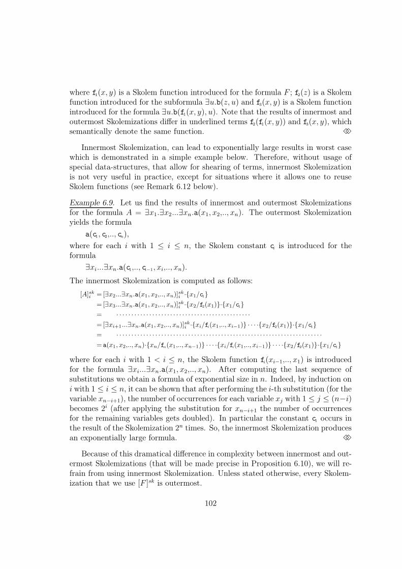
where f1(x, y) is a Skolem function introduced for the formula F ; f2(z) is a Skolemfunction introduced for the subformula ∃u.b(z, u) and f3(x, y) is a Skolem functionintroduced for the formula ∃u.b(f1(x, y), u). Note that the results of innermost andoutermost Skolemizations differ in underlined terms f2(f1(x, y)) and f3(x, y), whichsemantically denote the same function. 33

Innermost Skolemization, can lead to exponentially large results in worst casewhich is demonstrated in a simple example below. Therefore, without usage ofspecial data-structures, that allow for shearing of terms, innermost Skolemizationis not very useful in practice, except for situations where it allows one to reuseSkolem functions (see Remark 6.12 below).

Example 6.9. Let us find the results of innermost and outermost Skolemizationsfor the formula A = ∃x1.∃x2...∃xn.a(x1, x2,.., xn). The outermost Skolemizationyields the formula

a(c1, c2,.., cn),

where for each i with 1 ≤ i ≤ n, the Skolem constant ci is introduced for theformula

∃xi...∃xn.a(c1,.., ci−1, xi,.., xn).

The innermost Skolemization is computed as follows:

[A]ski =[∃x2...∃xn.a(x1, x2,.., xn)]sk

i ·{x1/c1}

=[∃x3...∃xn.a(x1, x2,.., xn)]ski ·{x2/f2(x1)}·{x1/c1}

= · · · · · · · · · · · · · · · · · · · · · · · · · · · · · · · · · · · · · · · · · · · · ·

=[∃xi+1...∃xn.a(x1, x2,.., xn)]ski ·{xi/fi(x1,.., xi−1)} · · · ·{x2/f2(x1)}·{x1/c1}

= · · · · · · · · · · · · · · · · · · · · · · · · · · · · · · · · · · · · · · · · · · · · · · · · · · · · · · · · · · · · · · · · · · · · ·

=a(x1, x2,.., xn)·{xn/fn(x1,.., xn−1)} · · · ·{xi/fi(x1,.., xi−1)} · · · ·{x2/f2(x1)}·{x1/c1}

where for each i with 1 < i ≤ n, the Skolem function fi(xi−1,.., x1) is introducedfor the formula ∃xi...∃xn.a(x1, x2,.., xn). After computing the last sequence ofsubstitutions we obtain a formula of exponential size in n. Indeed, by induction oni with 1 ≤ i ≤ n, it can be shown that after performing the i-th substitution (for thevariable xn−i+1), the number of occurrences for each variable xj with 1 ≤ j ≤ (n−i)becomes 2i (after applying the substitution for xn−i+1 the number of occurrencesfor the remaining variables gets doubled). In particular the constant c1 occurs inthe result of the Skolemization 2n times. So, the innermost Skolemization producesan exponentially large formula. 33

Because of this dramatical difference in complexity between innermost and out-ermost Skolemizations (that will be made precise in Proposition 6.10), we will re-frain from using innermost Skolemization. Unless stated otherwise, every Skolem-ization that we use [F ]sk is outermost.

102

Innermost and outermost Skolemizations can be mixed (some quantifiers canbe skolemized in innermost others in outermost way). This hybrid Skolemization isdenoted by [F ]skm (see the definition in subsection 6.3). The result of Skolemizationis not logically equivalent to the input formula, but preserves its (un)satisfiability.

Proposition 6.10. For any formula F ∈ [FO]nnf the result of mixed Skolemiza-tion [F ]skm (outermost Skolemization [F ]sko ) can be computed in exponential (poly-nomial) time in |F | such that the following holds: (i) [F ]skm is conservative over Fand (ii) |[F ]skm | ≤ (w + 1)e·|F |; |[F ]sko | ≤ (w + 1)·|F |, where w = width(F ) and eis the number of existential quantifiers in F .

Proof. In every computation of the function [F ]skm there are at most |F | recursivecall (exactly one for every logical connective in F , since a substitution does notchange any of those). Therefore the recursive function [·]skm always terminates.Since there are at most linear number of recursion calls, the computation time forSkolemization is mainly influenced by the (intermediate) sizes of formulas, whichwe estimate below.

To estimate the size of [F ]skm , note that during its computation exactly e substi-tutions have been applied to a formula (one for every existential quantifier). Everysubstitution increases the size of the formula in at most w +1 times (every Skolemfunction contains at most w variables). Therefore, the size of the result |[F ]skm | isbounded by (w + 1)e·|F |. For the outermost Skolemization, we can obtain a muchlower bound, since one could notice that Skolem functions cannot be nested in theresult [F ]sko . Indeed, according to the definition of [·]sko given in Figure 23, Skolemfunctions that are substituted for variables do not contain variables that will beinstantiated afterwards. So, the size of the result |[F ]sko | cannot exceed the value(w + 1)·|F |, which is polynomial in |F |. Hereby, we have proven the point (ii) ofProposition.

The bounds on the sizes of skolemized formulas imply that the procedure com-puting mixed (outermost) Skolemization can be implemented in exponential (re-spectively polynomial) time in the size of the input. It remains to show the point(i) of Proposition which we do by induction over [·]skm .

First, it can be shown that F is a logical consequence of [F ]skm . The base caseand induction steps for conjunction and disjunction is trivial. For the case witha universal quantifier, ∀y.F1 is a logical consequence of [∀x.F1]

skm = ∀x.[F1]

skm by

Replacement Lemma (see Lemma 2.4), since F1 is a logical consequence of [F1]skm

by induction hypothesis. For the case with an existential quantifier, ∃y.F1 is alogical consequence of the formula F1·{y/fF(x)}, which by induction hypothesis isa logical consequence of both [F1]

skm ·{y/fF(x)} and [F1·{y/fF (x)}]skm .

Now we prove that any model M of F can be expanded to a model M′ of[F ]skm . We expand any interpretation M by defining the interpretation of new

103

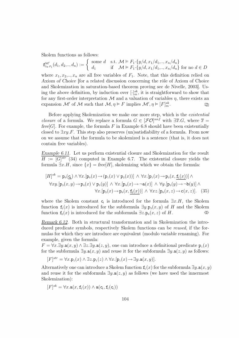
Skolem functions as follows:

fM′

∃y.F1(d1, d2,.., dn) :=

{some d s.t. M � F1·{y/d, x1/d1,.., xn/dn}d1 if M � F1·{y/d, x1/d1,.., xn/dn} for no d ∈ D

where x1, x2,.., xn are all free variables of F1. Note, that this definition relied onAxiom of Choice [for a related discussion concerning the rôle of Axiom of Choiceand Skolemization in saturation-based theorem proving see de Nivelle, 2003]. Us-ing the above definition, by induction over [·]skm , it is straightforward to show thatfor any first-order interpretation M and a valuation of variables η, there exists anexpansion M′ of M such that M, η � F implies M′, η � [F ]skm . 22

Before applying Skolemization we make one more step, which is the existentialclosure of a formula. We replace a formula G ∈ [FO]nnf with ∃x.G, where x =free[G]. For example, the formula F in Example 6.8 should have been existentiallyclosed to ∃xy.F . This step also preserves (un)satisfiability of a formula. From nowon we assume that the formula to be skolemized is a sentence (that is, it does notcontain free variables).

Example 6.11. Let us perform existential closure and Skolemization for the resultH := [G]str (34) computed in Example 6.7. The existential closure yields theformula ∃x.H, since {x} = free[H], skolemizing which we obtain the formula:

[H]sk = p0(c1) ∧ ∀x.[p0(x)→(p1(x) ∨ p2(x))] ∧ ∀x.[p1(x)→p3(x, f1(x))]∧

∀xy.[p3(x, y)→p4(x) ∨ p5(y)] ∧ ∀x.[p4(x)→¬a(x)] ∧ ∀y.[p5(y)→¬b(y)]∧

∀x.[p2(x)→p6(x, f2(x))] ∧ ∀xz.[p6(x, z)→c(x, z)]. (35)

where the Skolem constant c1 is introduced for the formula ∃x.H, the Skolemfunction f1(x) is introduced for the subformula ∃y.p3(x, y) of H and the Skolemfunction f2(x) is introduced for the subformula ∃z.p6(x, z) of H. 33

Remark 6.12. Both in structural transformation and in Skolemization the intro-duced predicate symbols, respectively Skolem functions can be reused, if the for-mulas for which they are introduce are equivalent (modulo variable renaming). Forexample, given the formula:F = ∀x.∃y.a(x, y)∧ ∃z.∃y.a(z, y), one can introduce a definitional predicate p1(x)for the subformula ∃y.a(x, y) and reuse it for the subformula ∃y.a(z, y) as follows:

[F ]str = ∀x.p1(x) ∧ ∃z.p1(z) ∧ ∀x.[p1(x)→∃y.a(x, y)].

Alternatively one can introduce a Skolem function f1(x) for the subformula ∃y.a(x, y)and reuse it for the subformula ∃y.a(z, y) as follows (we have used the innermostSkolemization):

[F ]sk = ∀x.a(x, f1(x)) ∧ a(c1, f1(c1))

104

where the Skolem constant c1 is introduced for the subformula ∃z.∃y.a(z, y). Thisre-usage technique can further refine the structural transformation and Skolemiza-tion which yield smaller CNF’s in many situations [see Nonnengart & Weidenbach,2001]. 33

6.4 Clausification

Clausification is probably the most expensive transformation in computation of aclause normal form. Like Skolemization it can produce exponentially large results,if not used carefully.

After Skolemization step we may assume that all existentially quantified vari-ables are eliminated and only universally quantified variables left (remember thatour formula is closed). We drop the universal quantifiers (first, renaming allbounded variables apart), since they do not carry any information anymore. Thus,we assume that all variables of the resulted expression are implicitly universallyquantified. The obtained formula has the following simple form:

P ::= L | F1 ∨ F2 | F1 ∧ F2 . (36)

where L ::= a(t1, t2,.., tn) | ¬a(t1, t2,.., tn) is a literal, that is, an atom or its nega-tion, whose arguments are first-order terms. Now an expression of the form (36) istranslated to a set of clauses using a clausification transformation. A quantifier-free first order formula F in negation normal form is in conjunction normal form(also denoted CNF since there is not much difference with clause normal form) ifany subformula of the form F1 ∨ F2 of F does not contain conjunctions. Duringthe clausification step, the conjunctions are repeatedly distributed over disjunc-tions using the following rewrite rules applied to subformulas of a formula:

A ∨ (B ∧ C) ⇒ (A ∨ B) ∧ (A ∨ C) and (A ∧ B) ∨ C ⇒ (A ∨ C) ∧ (B ∨ C)

There are different ways to show that this transformation terminates. The trans-formation rules above can be oriented using an LPO-ordering [see Bachmair &Ganzinger, 2001], however this does not give one any complexity bounds for thetransformation. In order to estimate the time spent on clausification and the size ofthe result, we compute the result [F ]cnf of CNF transformation using the function[· | ·]cnf defined in Figure 24. The function [· | ·]cnf is defined recursively over thefirst argument F ∈ P of the form (36). The second argument is used for bookkeep-ing a disjunction of literals that are cut from the formula F while decomposing it.

The main difficulty in proving termination of this function (and estimating itscomputational cost) arises in the last recursion step, which normalizes a formulamodulo associativity of disjunction. For this purpose we introduce a new weight

105

Figure 24 Clausification for quantifier-free first-order formulas

[F ]cnf := [F | ⊥]cnf ;

[F |C]cnf := [L |C]cnf = C ∨ L |

[F1 ∨ L |C]cnf = [C ∨ L]cnfF1 |

[F1 ∧ F2 |C]cnf = [F1 |C]cnf ∧ [F2 |C]cnf |

[F1 ∨ (F2 ∧ F3) |C]cnf = [F1 ∨ F2 |C]cnf ∧ [F1 ∨ F3 |C]cnf |

[F1 ∨ (F2 ∨ F3) |C]cnf = [(F1 ∨ F2) ∨ F3 |C]cnf .

|F |cnf := |L|cnf = 1 |

|F1 ∨ F2|cnf = |F1|cnf + |F2|1

cnf + 1 |

|F1 ∧ F2|cnf = |F1|cnf + |F2|cnf + 1 .

|F |1cnf := |L|1cnf = 1 |

|F1 ∨ F2|1cnf = |F1|

1cnf + |F2|

1cnf + 2 |

|F1 ∧ F2|1cnf = |F1|

1cnf + |F2|

1cnf + 1 .

function | · |cnf that is defined in Figure 24. The weight function |F |cnf sums theweights literals, conjunction and disjunction symbols in F . All these symbols havea weight 1 unless it is a disjunction symbol that appears inside the right disjunctF2 of some subformula F1 ∨ F2 of F . In this case the weight of the disjunctionsymbol is 2 (additional penalty is added for the occurrence in a right disjunct).For example, |(L1 ∨ L2) ∨ L3|cnf = 5, but |L1 ∨ (L2 ∨ L3)|cnf = 6, which makes itpossible to orient the last recursion step (associativity of disjunction). Using theweight function | · |cnf we show that clausification terminates in exponential timeand produces at most exponentially large CNF.

Proposition 6.13. For any formula F ∈ P defined according to (36), the result ofclausification S := [F ]cnf can be computed in polynomial time in 2|F | and producesa formula S in CNF such that (i) S ≡ F and (ii) |S| ≤ 2|F |.

Proof. First we show that for any formula F ∈ P there are at most 22·|F | recursivecalls of the function [· | ·]cnf possible during the computation of [F ]cnf . Observethat in every recursion call the weight of the first parameter strictly decreases:

|F1 ∨ L|cnf = |F1|cnf + |L|1cnf + 1 > |F1|cnf ;

|F1 ∧ F2|cnf = |F1|cnf + |F2|cnf + 1 > max(|F1|cnf , |F2|cnf);

|F1 ∨ (F2 ∧ F3)|cnf = |F1|cnf + (|F2|1cnf + |F3|

1cnf + 1) + 1 >

> |F1|cnf + max(|F2|1cnf , |F3|

1cnf) + 1 =

= max(|F1 ∨ F2|cnf , |F1 ∨ F3|cnf);

|F1 ∨ (F2 ∨ F3)|cnf = |F1|cnf + (|F2|1cnf + |F3|

1cnf + 2) + 1 >

> (|F1|cnf + |F2|1cnf + 1) + |F3|

1cnf + 1 = |(F1 ∨ F2) ∨ F3|cnf .

Note also that |F |cnf < 2·|F | for every F ∈ P.The computation tree for [F | ·]cnf is a binary tree: every recursion step fires at

most two recursive calls of the function [· | ·]cnf . On every branch of this tree thereare at most |F |cnf < 2·|F | recursion calls (the weight function cannot decrease

106

more than |F |cnf times). Therefore, the size of the recursion tree and the totalnumber of recursion calls used in computation of [F ]cnf is bounded by 22·|F |. Belowwe will show that the function produces the output of the size at most 2|F |. Thiswill imply that clausification can be computed in polynomial time in 2|F | (thepolynomial overhead is caused by manipulations with intermediate results, thatdepend on a data structure implementation).

Since we have proved that the function [· | ·]cnf terminates, we may use inductionover it. By such an induction now it is easy to show that the result of clausificationis equivalent to the input formula and has at most exponential size in the inputformula. More precisely, (i) [F |C]cnf ≡ C ∨F and (ii) |[F |C]cnf | < (|C|+2)·2|F |.This respectively imply the parts (i) and (ii) of Proposition. 22

Clausification of a formula F ∈ P produces a conjunction of disjunctions. Wedrop the conjunctions between disjunctions and view the result as sets of clauses.All clauses have implicitly disjoint variables (which are implicitly universally quan-tified), so we can reuse variable names.

Example 6.14. By applying clausification for the formula computed in Exam-ple 6.11, we obtain the following set of clauses:

p0(c1);¬p0(x) ∨ p1(x) ∨ p2(x);¬p1(x) ∨ p3(x, f1(x));¬p3(x, y) ∨ p4(x) ∨ p5(y);

¬p4(x) ∨ ¬a(x);¬p5(y) ∨ ¬b(y);¬p2(x) ∨ p6(x, f2(x));¬p6(x, z) ∨ c(x, z).

33

Remark 6.15. Although clausification is exponential in worst case (see example(31)), most translations that we give for fragments are polynomial. This is mainlybecause of the structural transformation step which is applied before clausification.Since the structural transformation produces a formula of the form (33), we need toperform clausification only for conjuncts of these formula, which have a fixed formfor a fragment. Therefore, every conjunct is translated into CNF with a linearoverhead in the size and clausification can be computed in polynomial time. 33

6.5 Summary for CNF-Transformations

Complexity estimations for the steps of CNF-transformation are summarized inTable 1. As seen from the table, the most expensive steps of the transformationare Skolemization and clausification, which are exponential in worst case. Notethat this does not really imply that CNF-transformation is doubly exponential inworst case, since Skolemization produces possibly exponentially large literals, but

107

Table 1 Summary for complexity of CNF transformations\Transformation NNF Structural Ex. Closure Skolemization Clausification

Complexity\ 99K [ ]nnf99K 99K [ ]str99K F 99K∃x.F 99K [ ]sk99K 99K [ ]cnf99K

Size 2·|F | O(w·|F |) w + |F |(w + 1)e·|F |

(w + 1) · |F |∗2|F |

O(|F |)†

Time p(|F |) p(|F |) p(|F |)p((w + 1)e·|F |)

p(|F |)∗p(2|F |)p(|F |)†

where w = width(F ); ∗for outermost Skolemizatione = the number of existential quantifiers in F ; †in combination with structuralp(·) is a polynomial function. transformation

leaves the number of boolean connectives polynomial, whereas clausification expo-nentially increases the number of boolean connectives leaving literals unchanged.Thus, the result of CNF-transformation is at most exponential in the size of theinput formula.

In decision procedures one typically employs polynomial CNF-transformation.This is achieved by (i) using the outermost skolemization and (ii) applying thestructural transformation before clausification step (see Remark 6.15). In fact,in most procedures, CNF-transformation produces a result of the size O(w·|F |),where w is the width of the input formula F .

108

7 The Theorem Proving Process

In this section we revisit the saturation process considered in subsection 3.4. So far,saturation process has been described from an abstract viewpoint (see Figure 5),now we address it from pragmatic side. We discuss how a saturation-based strategycan be implemented. Here we mainly address the following two questions: (1) howredundancy can be practically used in theorem provers and (2) how deductionof clauses can be organised in a fair way? In order to answer these and otherquestions, we consider a simple model of a saturation-based theorem prover. Thismodel will be used for deriving complexity bounds for decision procedures that wepresent afterwards.

7.1 Simplification Rules

The calculi introduced in previous sections form a core inference system in saturation-based theorem provers. The inference rules of these calculi are usually called thededuction rules. Besides deduction rules, most calculi employ additional simplifi-cation rules during a saturation process. Simplification rules implement deletion ofredundant clauses and clause rewriting (i.e., replacing clauses with simpler ones).Their purpose is to keep the search space of a theorem prover manageable, i.e.,to keep as small number of clauses as possible. In fact, modern theorem proverssuch as Vampire [Riazanov & Voronkov, 2002] or Spass [Weidenbach et al., 2002],spend most of their computation time on simplification and not on deduction.

The general form of simplification rules that we consider in this report is spec-ified by

A Simplification Rule

SR :S ∪ [[S ′ ]]

S1 || · · · || Sn

where the conditions of the rule hold

(37)

where S, S ′, S1, .., Sn are clause sets. Some premises of a simplification rule mightbe enclosed in brackets [[···]], which means that they should be deleted after thisinference is applied. Simplification rules might be multi-conclusion, i.e., possiblyseveral clauses can be produced in an inference. We also admit nondeterminis-tic inference rules, i.e., when there are several choices between conclusions of aninference rules called the possible conclusions of the rule (here we separate thesechoices with || ).

Definition 7.1 (Admissible Simplification Rules).We say that a simplification rule R : S ∪ [[S ′ ]] ` S1 || · · · || Sn is sound if every

109

model for S ∪ S ′ is a model for some Si with 1 ≤ i ≤ n. R is compatible with aredundancy criterion R = (RCl(·), RInf (·)) if for every i with 1 ≤ i ≤ n, we haveS ′ ⊆ RCl(S ∪ Si). Finally, we say that a simplification rule R is admissible for acalculus C based on a redundancy criterion R if R is sound and compatible withR. 33

Soundness of simplification rules is required to ensure that a rule can be alwaysapplied such that it preserves satisfiability of a clause set. Additionally, deletion ofpremises must be performed according to a redundancy criterion in order to retainrefutational completeness. In other words, application of simplification rules shouldnot prevent from deriving the empty clause from an unsatisfiable clause set. Thetype of nondeterminism in simplification rules is a “don’t know ” nondeterminism,meaning that only a certain choice of possible conclusions (which is a-priori notknown) preserves satisfiability of a clause set. This makes a saturation process alsonondeterministic (i.e., with backtracking).

Figure 25 Some simplification rules used in saturation-based theorem provers

Tautology Deletion Elimination of Duplicate Literals

TD :[[C ∨ A ∨ ¬A ]]

ED :[[C ∨ L ∨ L ]]

C ∨ L

— —

Subsumption Deletion Splitting

SD :C [[D ]]

SP :[[C ∨ D ]]

C || D

where (i) C strictly subsumes Dwhere (i) C 6= �; (ii) D 6= � and(iii) vars[C] ∩ vars[D] = {}.

In figure 25 we list some simplification rules which are often used in saturation-based theorem provers.18 We have already discussed several times the impact oftautology deletion on refutational completeness of some calculi. The TautologyDeletion rule implements deletion of simple syntactical tautologies. This rule isapplied to a clause that has complementary literals and does nothing except thatit deletes this clause. Another similar simplification rule is Elimination of DuplicateLiterals, which is applied to a clause that has multiple occurrences of some literaland replaces it with a clause in which duplicate occurrences of this literal areremoved. The Subsumption Deletion rule is applied to two clauses, one of whichstrictly subsumes the other. This rule does not produce any conclusion, but deletes

18See [Weidenbach, 2001] for a variety of other simplification rules that are commonly used insaturation-based theorem provers

110

the subsumed clause. Finally, the Splitting rule is applied to a clause C ∨ D thatconsists of two non-empty variable disjoint parts C and D. If such a clause is truein a model, then either C must be true or D must be true in this model. This ruleimplements this nondeterministic choice and deletes the premise of this rule. It iseasy to check that all simplification rules from Figure 25, are admissible accordingto Definition 7.1 w.r.t. the standard redundancy criterion with subsumption (seeAppendix A.2).

7.1.1 Simplification rules extending a signature

For some saturation-based decision procedures we need to employ simplificationrules that might extend a signature. An example of such inference rules is thefollowing rule:

Splitting through New Predicate Symbol

SPP :C ∨ D

C ∨ uC(x)

D ∨ ¬uC(x)

where (i) C 6= �; (ii) D 6= �; (iii) vars[C]∩vars[D] = xand (iv) u

Cis an extended predicate symbol introduced

for C.

(38)

This simplification rule splits a clause consisting of two subclauses C and D byintroducing a new predicate symbol u

C(x) over common variables of these sub-

clauses. In case when uC(x) is sufficiently small in the ordering, the premise of

this rule becomes redundant w.r.t. to the conclusions of this rule (obviously, thepremise logically follows from the conclusions of this rule). An instance of Splittingthrough New Predicate Symbol, when C and D do not have variables in common,has been considered in [Riazanov & Voronkov, 2001; de Nivelle, 2001] for sim-ulating the Splitting rule and to avoid backtracking in saturation-based theoremprovers.

In order to integrate such inference rules in our framework, we assume thatfor every extended predicate or functional symbol u that might be introduced bya simplification rule, there is a function that given a first-order interpretation Iover the initial signature, expands this interpretation to new signature elements. Inother words, interpretation of base elements of a signature, uniquely determines theinterpretation for every extended element. We will denote by uI the interpretationof the symbol u under this expansion of I.

Extension of interpretations for introduced predicate symbols can be done bysupplying first-order definitions for them. For example, formula u

C(x) above can

111

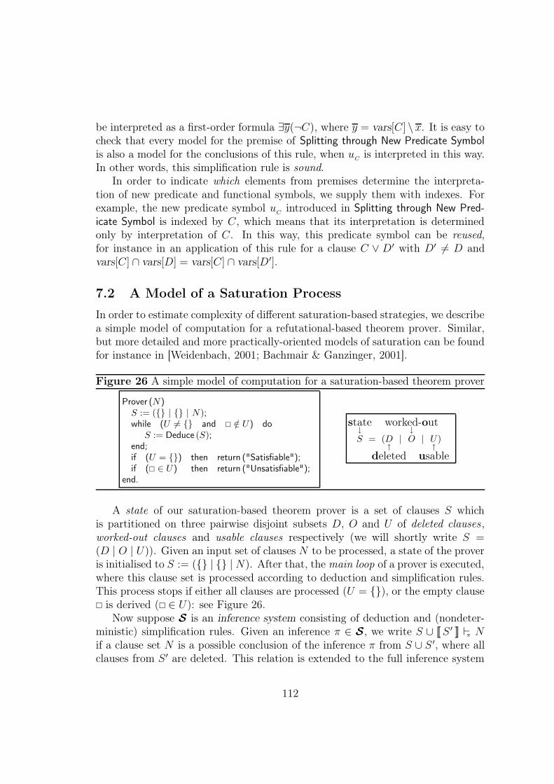
be interpreted as a first-order formula ∃y(¬C), where y = vars[C] \x. It is easy tocheck that every model for the premise of Splitting through New Predicate Symbolis also a model for the conclusions of this rule, when u

Cis interpreted in this way.

In other words, this simplification rule is sound.In order to indicate which elements from premises determine the interpreta-

tion of new predicate and functional symbols, we supply them with indexes. Forexample, the new predicate symbol u

Cintroduced in Splitting through New Pred-

icate Symbol is indexed by C, which means that its interpretation is determinedonly by interpretation of C. In this way, this predicate symbol can be reused,for instance in an application of this rule for a clause C ∨ D′ with D′ 6= D andvars[C] ∩ vars[D] = vars[C] ∩ vars[D′].

7.2 A Model of a Saturation Process

In order to estimate complexity of different saturation-based strategies, we describea simple model of computation for a refutational-based theorem prover. Similar,but more detailed and more practically-oriented models of saturation can be foundfor instance in [Weidenbach, 2001; Bachmair & Ganzinger, 2001].

Figure 26 A simple model of computation for a saturation-based theorem prover

Prover (N)S := ({} | {} | N);while (U 6= {} and � /∈ U) do

S := Deduce (S);end;if (U = {}) then return ("Satisfiable");if (� ∈ U) then return ("Unsatisfiable");

end.

state↓

S = (D↑

deleted

|

worked-out↓

O | U↑

usable

)

A state of our saturation-based theorem prover is a set of clauses S whichis partitioned on three pairwise disjoint subsets D, O and U of deleted clauses,worked-out clauses and usable clauses respectively (we will shortly write S =(D | O | U)). Given an input set of clauses N to be processed, a state of the proveris initialised to S := ({} | {} | N). After that, the main loop of a prover is executed,where this clause set is processed according to deduction and simplification rules.This process stops if either all clauses are processed (U = {}), or the empty clause� is derived (� ∈ U): see Figure 26.

Now suppose S is an inference system consisting of deduction and (nondeter-ministic) simplification rules. Given an inference π ∈ S, we write S ∪ [[S ′ ]] π Nif a clause set N is a possible conclusion of the inference π from S ∪ S ′, where allclauses from S ′ are deleted. This relation is extended to the full inference system

112

by writing S ∪ [[S ′ ]] S N when N is the set of all clauses that are obtained in onestep from clauses S ∪ S ′ and S ′ is the set of all clauses that were deleted in theseinferences, i.e., formally:

S∪[[ S ′ ]] S N iff N =⋃

π∈S

Nπ; S ′ =⋃

π∈S

S ′π; where S∪S ′\S ′

π∪[[ S ′π ]] π Nπ. (39)

In order to explain how deduction takes place, we need to introduce additionaloperation with theorem proving states, namely insertion of clauses. Given a the-orem proving state S = (D | O | U), the result of insertion of a clause set Ninto S is a theorem proving state defined by: S ∪ N = (D | O | U) ∪ N :=D | O | (U ∪ N \ (D ∪ O)). It is obvious that insertion preserves disjointnessfor the sets of deleted, worked-out and usable clauses. Now the transformationDeduce(S) performing deduction of new clauses in the main loop of a prover isdefined in Figure 27 According to this definition, the next theorem proving state is

Figure 27 Deduction of new clauses

DeduceD | O t O′ | {C} t U ⇒ (D ∪ O′ | O ∪ {C} | U) ∪ N where O ∪ {C} ∪ [[O′ ]] S N

D | O t O′ | {C} t U ⇒ (D ∪ O′ ∪ {C} | O | U) ∪ N where O ∪ [[ {C} ∪ O′ ]] S N

obtained from the previous state by (1) selecting a usable clause, (2) inserting con-clusions of all inferences between this clause and worked-out clauses, (3) movingdeleted clauses into D and (4) moving the selected clause into the set of worked-out clauses O if it has not been deleted. Note that the Deduce transformationmight be nondeterministic, since the relation S is not necessary functional be-cause of nondeterministic simplification rules. However, if all simplification rulesare deterministic, then the saturation procedure is also deterministic.

In our model of saturation, deleted clauses are not removed from a clause set,but moved into a special set D of deleted clauses (speaking in deferent terms, theseclauses are marked as deleted). This is done to implement a so-called permanentdeletion. Using permanent deletion, clauses that were once deleted, are memo-rised in a theorem proving state which prevents it from deriving them again. Thishelps avoiding (infinite) repetitions of deriving/deletion of the same clauses andsolves certain problems with fairness of a saturation process. However, permanentdeletion requires more memory.19 For certain inference rules, like Tautology Dele-tion or Elimination of Duplicate Literals it is possible to completely remove deletedpremises, when these inference rules are applied eagerly. Eager application of asimplification rule means that the rule is applied to a clause set as soon as it has

19This is a reason why most of theorem provers do not use permanent deletion and solveproblems with fairness by different means

113

become applicable. In this case, all clauses are kept normalised w.r.t. these rules.For example, eager application of Elimination of Duplicate Literals, amounts to dele-tion of all duplicate literals in clauses that are produced. The only requirement foreager application, is that this normalisation process must always terminate. It ispossible to show that, in fact, all simplification rules from Figure 25 can be usedeagerly, i.e., saturation of every clause set w.r.t. these inference rules always ter-minates (indeed, conclusions of these inference rules have a strictly smaller literalsthan their premises).

In Figure 28, we modified the computational model from Figure 26 to make useof eager simplification rules. For this, we have defined an additional transforma-tion Simplify(S) for states of a prover. This transformation performs all one-step

Figure 28 A model of computation with eager simplification rules

Prover (N)S:=Normalise ({} | {} | N);while (U 6= {} and � /∈ U) do

S:=Normalise (Deduce (S));end;if (U = {}) then return ("Satisfiable");if (� ∈ U) then return ("Unsatisfiable");

end.

Normalise (S)repeat

S′:= S;S := Simplify (S′);

until (S = S′);return(S);

end.

SimplifyD | O t O′ | U t U ′ ⇒ (D ∪ O′ | O | U) ∪ N where O ∪ U ∪ [[O′ ∪ U ′ ]] Se

N

inferences from the set of worked-out and usable clauses w.r.t. the set Se of eagersimplification rules of an inference system. If a worked-out clause is deleted duringany of these inferences, than it is moved into the set D of deleted clauses. On theother hand, all deleted usable clauses are simply removed from a clause set. Thistransformation is iteratively repeated until nothing new is derived or deleted. Thedescribed procedure is implemented using function Normalise(S), which is appliedin a state of a prover after each deduction step.

7.2.1 Correctness of the theorem-proving procedures

Before using the procedures given in Figure 26 and Figure 28, we have to demon-strate their correctness. That is, we need to show their (1) soundness: for everysatisfiable input set N there is a branch where a prover does not return "Unsat-isfiable", and (2) completeness: for every unsatisfiable input set N a prover mustreturn "Unsatisfiable".

Soundness for a theorem prover follows from soundness of inference rules be-cause the Deduce and the Simplify transformations can be always applied in a

114

satisfiability-preserving way. For showing completeness, we need to make addi-tional assumptions about the data structure used to operate with sets of clauses(to ensure, in particular, that the results of different operations can be alwayscomputed). We assume that there is an efficient mechanism that provides for:

1. Insertion of clauses: Given a theorem proving state S, the result of inser-tion of a clause set N into S can be effectively computed.

2. Enumeration of clauses: For every state S = (D | O | U), the sets O andU of worked-out and usable clauses can be effectively enumerated.

3. Fair selection of usable clauses: There is a function Choose(·) that givena theorem proving state S = (D | O | U) selects a usable clause Choose(S) ∈ Usuch that for every sequence of theorem proving states Si = (Di | Oi | Ui),i = 1, 2,.., n,.., with Choose(Si) /∈ Uj when 1 ≤ i < j, we have

⋃i≥1

⋂j≥i Uj =

{}. In other words, if selected clauses are permanently removed from the setof usable clauses, then every usable clause will be eventually removed.

The first property can be achieved by keeping the set of all clauses sorted, andchecking whether a clause is already in this set during insertion. In this way,insertion of each clause C in a state S can be done in time O(|C|). For the secondproperty, one can use links to the “next” and “previous” elements in O and U . Thethird property can be implemented in various ways, for instance, by assigning toevery new clause a positive weight (say, the number of symbols in a clause) andselecting a minimal new clause according to this weight [see Weidenbach, 2001].

Properties 1 and 2 above insure that one can always compute the results oftransformations Deduce and Simplify. It is easy to see that every state S computedin saturation process contains all inferences from the set O of worked-out clauses.Since deletion of clauses is done according to a redundancy criterion, all clausesfrom D must be redundant w.r.t. S.

Note that rules Deduce and Simplify are instances of theorem proving derivationsgiven in Figure 5. Hence, the limit of every sequence S1 \ D1, S2 \ D2, · · · ofnon-deleted clauses from theorem proving states, is saturated up to redundancyprovided that all derivations were performed fairly (see Definition 3.24 on p. 47). Inthis case, completeness of our theorem prover follows from Completeness Criterion(see Corollary 3.28).

Fairness of derivations is guaranteed by assumption 3 above. Indeed, if someinference π can be applied to all Si\Di starting from some j ≥ 1, then by condition3, there exists k ≥ j such that Ok contains all premises of π. Hence the conclusionof π must be in Sk, and so π is redundant w.r.t. Sk \ Dk.

115

7.2.2 Complexity of saturation procedures

In many saturation-based decision procedures it is possible to estimate the maximalnumber of different clauses that might be produced by a saturation procedure. Thisgives a bound on space complexity of decision procedures. We will use the modelof theorem prover given in Figure 28 to estimate the time required to compute asaturation of bounded size.

We assume that the conclusion of every inference can be computed in polynomialtime in the size of its premises. This assumption holds for all calculi introducedin this chapter. Moreover, we assume that normalisation of a clause set N w.r.t.eager simplification rules can be done in polynomial time in the size of N . Formany simplification rules and clause classes this is indeed the case. It is possibleto show that normalisation w.r.t. Tautology Deletion, Elimination of Duplicate Lit-erals and Splitting can be done in polynomial time. Checking subsumption is ingeneral an NP-complete problem [see Garey & Johnson, 1979], however for clauseswith bounded number of literals containing all variables of a clause, SubsumptionDeletion can be done in polynomial time [Gottlob & Leitsch, 1985; Ganzinger &de Nivelle, 1999]. In other cases, this rule can be always replaced with a suitablepolynomial approximation [see Weidenbach, 2001].

We give estimation for time complexity of saturation procedures in terms of:

|N | - the size of the initial clause set;

c - the maximal number of normalised clauses;

s - the maximal number of clauses in a normalised clause set;

m - the maximal size of a normalised clause;

k - the maximal number of premises in all deduction and simplificationrules.

Note that s bounds the number of worked-out and usable clauses after each nor-malisation steps, whereas c bounds the total number of clauses (including deletedones) after normalisation. The value s might be strictly smaller than c, if thereare eager simplification rules with at least two premises. For example, if we useSubsumption Deletion eagerly, then s bounds the maximal number of clauses in aset where no clause strictly subsumes other clauses.

Now we estimate the time required to compute a saturation according to theprocedure from Figure 28. Normalisation of the input clause set can be done ittime p(|N |) (where p(·) is a polynomial function). In order to estimate the timerequired for the main loop, note that after each iteration of this loop, the setD ∪ O is incremented exactly on one clause, namely the usable clause which wasselected in the Deduce transformation. Since the total number of clauses in S afternormalisation step is bounded by c, we may have at most c iterations of the mainloop. In each iteration, according to Figure 27, one should compute all possible

116

inferences between worked-out clauses and the selected clause. The number ofsuch inferences is bounded by O(s(k−1)) (recall that the set of worked-out clausesis normalised before this step, hence their total number is bounded by s). Sinceevery inference can be done in polynomial time in m, the computational cost forthe Deduce step is O(s(k−1) ·p(m)), which is also a bound on the size on new clausesthat are derived in this step. The subsequent normalisation step can be done inpolynomial time in this value. Hence the total running time for the saturationprocedure is bounded by:

t = p(|N |) + c · p(m · s(k−1)) (40)

The estimation (40) for the time required to compute a saturation, can possi-bly be refined further, by considering a more detailed model of a theorem proverlike say in [Weidenbach, 2001]. However, the main message of this section is thatthe time complexity for saturation procedures is polynomial in its space complexity(under the given assumptions about complexity of inference rules). One shouldremember, however, that a saturation procedure can be nondeterministic, hencealthough non-deterministic space complexity classes coincide with correspondentnon-deterministic classes (for PSPACE or higher), this is not true for time com-plexity classes.

117

A Technical Appendixes

A.1 Lifting and Redundancy with Selection Functions

In this appendix we describe a completeness proof for the ordered resolution cal-culus with selection functions OR�

Seldefined in subsection 3.6 in System 7. We

also give formal definitions of redundancy criteria for non-ground calculi.

A.1.1 Abstract calculi and approximations

Before introducing a technique for proving completeness of OR�Sel, we consider the

lifting procedure described for OR� in section 3 from a more abstract viewpoint.

Definition A.1 (Calculus).An (abstract) calculus is a quadruple C = (L, P , Sp,Rp), where:

1. L = (D, �L, TL) is a logic, where D is a nonempty set called the domain;�L ∈ D is a basic contradiction, and TL ⊆ 2D is a collection of satisfiablesets that enjoys the following properties: (i) D1 ⊆ D2 ∈ TL implies D1 ∈ TL

and (ii) {�L} /∈ TL;

2. P is a non-empty set of admissible parameters of the calculus and for eachp ∈ P :

3. Sp ⊆ InfD := {(d1,.., dk ` d) | di, d ∈ D, 1 ≤ i ≤ k ≥ 0} is an inferencesystem and

4. Rp = (RpCl(·), R

pInf (·)) is a redundancy criterion, where for every D ⊆ D we

have RpCl(D) ⊆ D is the set of redundant clauses w.r.t. D and R

pInf (D) ⊆ InfD

is the set of redundant inferences w.r.t. D, are such that the analogs ofconditions in Definition 3.20 hold:

for every D \ D′ ⊆ RCl(D), (R1) D /∈ TL implies D′ /∈ TL, (R2) RCl(D) ⊆RCl(D

′) and (R3) RInf (D) ⊆ RInf (D′). R is effective if in addition (R4) π ∈

RInf (D) for every π ∈ InfD with π(d) ⊆ D.

The basic notions for inference systems and redundancy criteria from the defini-tions 2.39, 2.40, 3.24 and 3.26 are easily modified for abstract calculi. A clause setN is called C-saturated if N is (Sp,Rp)-saturated for some p ∈ P . The calculusC is (refutationally) complete if for every p ∈ P , (Sp,Rp) is complete for D. 33

For example, the (ground version) of the ordered resolution calculus with selec-tion OR0�

Sel is a calculus based on the ground clause logic, i.e., L := (Cl0Σ, �, {N ⊆Cl0

Σ| N is satisfiable}). For simplicity, we identify the set of (ground) clauses with

118

the correspondent logic (i.e., here L = Cl0Σ). OR0�Sel is parametrized by the set

P := {(�, Sel) | “�” is admissible} of admissible orderings and selection func-tions. For every choice of a parameter p = (�, Sel) ∈ P , the inference systemSp := OR0�

Selis defined in System 5 and Rp := R

S�gr is the standard redundancy

criterion for ground clauses. The calculus OR0�Sel

is complete because, as it wasshown in Corollary 3.30, (Sp,Rp) is complete for any choice of admissible param-eters. Similarly, OR� is a calculus for the logic L := ClΣ and is parametrized byP := {� | “�” is admissible}. It is complete by Theorem 3.39.

The completeness criterion formulated in Corollary 3.28 can be extended with-out considerable modifications to abstract calculi as follows:

Lemma A.2 (Completeness Criterion for Calculi). Let C = (L, P , Sp,Rp)be a calculus. Then C is complete iff for every C-saturated set D ⊆ D, if D /∈ TL

then �L ∈ D.

This criterion motivates the following definition, using which it is possible totransfer completeness of one calculus to completeness of the other calculus:

Definition A.3 (Approximates). Given calculi C = (L = (D, �L, TL), P , Sp,Rp)and C′ = (L′ = (D′, �L

′, TL′), P ′, S ′

p,R′p), we say that C approximates C′ if there

exists a function α : 2D 7→ 2D′

such that for every D ⊆ D: (i) D is C-saturatedthen α(D) is C′-saturated, (ii) D /∈ TL implies α(D) /∈ TL

′ and (iii) �L /∈ Dimplies �L

′ /∈ α(D). 33

Definition A.3 is derived from the concept of approximation between theoremproving systems that has been introduced in [Bachmair et al., 1994] to reducerefutational completeness from one system to the other. In Theorem 3.39 wehave shown that the calculus OR� approximates its ground version OR0� via themapping gr : N 7→ N gr. This in the end made it possible to transfer completenessof OR0� to completeness of OR�. The arguments used in this proof can begeneralized to the following

Lemma A.4 (Relative Completeness). Let C = (L, P , Sp,Rp) be a calculusthat approximates a calculus C ′ = (L′, P ′, S ′

p,R′p) via α. Then C is complete if C ′

is complete.

Proof. Assume that C′ is complete but C is not. By the completeness criterion forcalculi (Theorem A.2), the last means that there exists a C-saturated set D ⊆ D

such that D /∈ TL and �L /∈ D. Since C approximates C′ via α, we have (i) α(D) isC′-saturated, (ii) α(D) /∈ TL

′ and (iii) �L′ /∈ α(D). However by the completeness

criterion for C′ from (i) and (ii) it follows that �L′ ∈ α(D). A contradiction with

(iii). 22

119

A.1.2 Ground closures

After these preparations, we demonstrate how to establish completeness of theordered resolution calculus with selection OR�

Sel. For this purpose, we introduce

an intermediate calculus ORgc�Sel

and show that OR�Sel

approximates ORgc�Sel

whichapproximates OR0�

Sel. This would imply from Corollary 3.30 by Lemma A.4 thatOR�

Selis complete.

The key concept of the intermediate calculus ORgc�Sel

is the notion of a groundclosure.

Definition A.5 (Ground Closures). A ground (clause) closure is a pair (C 0:C),where C ∈ ClΣ is a clause and C 0 = Cσ ∈ Cl0

Σis a ground instance of C. The set

of all ground closures over a signature Σ is defined by GCΣ.Given a clause set N ⊆ ClΣ, we define Ngc := {(C 0:C) ∈ GCΣ | C ∈ N} to be

the set of all ground closures for clauses in N . For a subset M ⊆ GCΣ, we denoteby Mgr its ground part, i.e., M gr := {C 0 | (C 0: C) ∈ N}. Note that N gr = (Ngc)gr

for all N ∈ ClΣ.A set M ⊆ GCΣ of ground closures is satisfiable if M gr is satisfiable. The logic

of ground closures is given by (GCΣ, (�: �), {M ⊆ GCΣ |M is satisfiable}) which wealso denote by GCΣ. 33

Along with the introduced notation for ground closures, we also write closuresof the form (C 0∨A0:C∨A) and (D0∨¬B0: D∨¬B) respectively as (C 0: C)∨(A0:A)and (D0:D) ∨ ¬(B0: B). However note, that for two ground closures (C 0: C) and(D0: D), the expression (C 0 ∨ D0: C ∨ D) is not necessary a ground closure, if Cand D have shared variables.

The intermediate calculus ORgc�Sel

is based on the logic of ground closures GCΣ

and is parametrized by an admissible ordering � on ground literals and a selectionfunction Sel on (full) clauses. The inference rules for any choice of these parametersare given in System 13. It can be easily shown (see the lifting diagram on Figure 7),

Ordered Resolution Ordered Factoring

OR :(C0: C) ∨ (A0: A)

?(D0: D) ∨ ¬(A0: B)

(C0: Cσ) ∨ (D0: Dσ)OF :

(C0: C) ∨ (A0: B) ∨ (A0: A)

(C0: Cσ) ∨ (A0: Aσ)

where (i) σ = mgu(A, B); (ii) A0 is strictlymaximal w.r.t. C 0 and nothing is selected in C∨A,and (iii) either ¬B is selected in D ∨ ¬B, or,otherwise nothing is selected in D ∨ ¬B and ¬A0

is maximal w.r.t. D0

where (i) σ = mgu(A, B); (ii) A0 ismaximal w.r.t. C 0 ∨ B0 and nothing isselected in C ∨ A ∨ B.

System 13: The intermediate calculus ORgc�Sel

for OR�Sel

that the set of ground closures is closed under inferences of this calculus. Moreover,

120

it is easy to see that for every inference π′ = [(C 01 :C1),.., (C

0k:Ck) ` (C 0:C)] ∈

ORgc�Sel

there exists a correspondent inference π = (C1,.., Ck ` C) ∈ OR�Sel

. Sothe lifting diagram can be extended for OR�

Sel and ORgc�Sel

: See the upper part inFigure 29. We exploit this correspondence for defining the notion of redundancy

Figure 29 The lifting diagram for OR�Sel

OR�Sel

:

ORgc�Sel

:

OR0�Sel′

:

C ∨ A?, D ∨ ¬B Cσ ∨ Dσ

(C0 ∨ A0?:

:C ∨ A?),(D0 ∨ ¬A0:

:D ∨ ¬B)(C0 ∨ D0::Cσ ∨ Dσ)

C0 ∨ A0?, D0 ∨ ¬A0 C0 ∨ D0

__gc

��

__gr

��

__

gc��

__

gr��

OR+3

OR +3

OR +3

C ∨ B ∨ A Cσ ∨ Aσ

(C0 ∨ A0 ∨ A0::C ∨ B ∨ A)

(C0 ∨ A0::Cσ ∨ Aσ)

C0 ∨ A0 ∨ A0 C0 ∨ A0

__

gc��

__

gr��

__

gc��

__

gr��

OF+3

OF +3

OF +3

for calculi parametrized by selection functions.

Definition A.6 (Standard Redundancy with Selection Functions). Let �be an ordering on ground literals that is admissible according to Definition 3.4. Theordering � on ground clauses is extended to ground closures by setting (C 0:C) �(D0: D) iff C 0 � D0. The logical entailment relation � is extended to the set ofground closures as follows: M1 � M2 iff Mgr

1 �Mgr2 .

Let S be an inference system on clauses and S ′ be a correspondent (via alifting diagram) inference systems on ground closures, both parametrized withthe same admissible ordering � and a selection function Sel. Given a set ofground closures M , we say that a ground closure (C 0: C) is redundant w.r.t. M ,if M(C0 :C) �(C 0: C).20 An inference π′ : (C 0

1 : C1),.., (C0

k: Ck) ` (C 0:C) ∈ InfGCΣ

is redundant w.r.t. M in S ′, if π′ ∈ S ′ implies that M(C0i :Ci) �(C 0: C), for some i

with 1 ≤ i ≤ k.Given a clause set N , we say that a clause C is redundant w.r.t. N if every

clause in {C}gc is redundant w.r.t. N gc. An inference π = C1,.., Ck ` C ∈ InfΣ isredundant w.r.t. N in S, if every ground closure (π0: π) := (C 0

1 : C1),.., (C0k: Ck) `

(C 0: C) ∈ InfGC of π is redundant w.r.t. N gc in S ′. 33

To summarise this definition in a practically usable way, a clause C is redun-dant w.r.t. N if every closure (C 0: C) of this clause is redundant w.r.t. the setof ground closures N gc of N , which is when the clause C 0 follows from the set((Ngc)(C0:C))

gr = (Ngr)C0 of the smaller ground instances from N gr. An inferenceπ ∈ S is redundant if every ground closure (π0: π) of this inference is redundant

20As usual, for a set D ⊆ D, ordered by � and d ∈ D, we denote Dd := {d′ ∈ D | d′ ≺ d}

121

w.r.t. Ngc, which is when either (π0: π) /∈ S ′ (this is only possible if π0 does notsatisfy the ordering restrictions for non-selected literals in π), or the conclusionC 0 of π0 follows from the set ((N gc)(C0

i :Ci))gr = (Ngr)C0

iof smaller clauses for some

premise C 0i of π0.

Note that the notions of redundant clauses and redundant inferences given inDefinition A.6, coincide with those given in Definition 3.36, when the selectionfunction is trivial: Sel = Sel0. So, ground closures are essentially needed fordefining redundancy of inferences having selected literals. In the next section, weshow how ground closures allow to refine the notion of redundancy even further.

Lemma A.7 (Standard Redundancy Criterion for Ground Closures). Thenotion of standard redundancy R

S′�

gc = (R�GC(·), RS

′�InfGC

(·)) for ground closures given

in Definition A.6 is a redundancy criterion for every inference system S ′ on groundclosures and a well-founded ordering � on ground clauses. If in addition S ′ ismonotone w.r.t. �, then R

S′�

gc is effective.

Proof. The proof of this lemma is identical to the proof of Lemma 3.21, but forground closures instead of ground clauses. 22

Corollary A.8 (Standard Redundancy Criterion with Selection Func-tions). The extension of the notion of standard redundancy R

S� = (R�Cl(·), R

S�Inf (·))

for inference systems with selection functions given in Definition A.6 a redundancycriterion. In addition, if the correspondent inference system S ′ on ground closuresis monotone, then R

S� is effective.

Proof. Similarly as in the proof of Lemma 3.37, this corollary follows from the factthat for every clause sets N ′ and N , we have N ⊆ R

�Cl(N) iff Ngc ⊆ R

�GC(Ngc), and

for every set of inferences S ⊆ InfΣ, we have S ⊆ RS�Inf (N) iff Sgc ⊆ R

S′�

InfGC(Ngc),

where Sgc ⊆ InfGCΣis the set of all ground closures of inferences in S. 22

Lemma A.9. OR�Sel

approximates ORgc�Sel

.

Proof. We show that the mapping gc : N 7→ N gc, N ⊆ ClΣ is an approximationfunction for OR�

Seland ORgc�

Sel. First note that conditions (ii) and (iii) for ap-

proximations (see Definition A.3) are trivial by definition of the logic for groundclosures (see Definition A.5). In order to demonstrate (i), let N be a clause setthat is saturated in OR�

Selunder some ordering � and selection function Sel. We

show that the set N gc is saturated in ORgc�Sel

under the same parameters. Indeed,for every inference π′ = [(C 0

1 :C1),.., (C0k:Ck) ` (C 0: C)] ∈ ORgc�

Selthere exists a cor-

respondent inference π = (C1,.., Ck ` C) ∈ OR�Sel

. Moreover, by Definition A.6,if π is redundant w.r.t. N then π′ is redundant w.r.t. N gc. Hence the set N gc issaturated in ORgc�

Sel. 22

122

Lemma A.10. ORgc�Sel

approximates OR0�Sel.

Proof. We show that the mapping gr : M 7→ M gr, M ⊆ GCΣ is an approximationfunction for ORgc�

Seland OR0�

Sel. Again, conditions (ii) and (iii) follow from thedefinition of the logic for ground closures. In order to demonstrate (i), let M bea saturated in ORgc�

Selset under some ordering � and selection function Sel. We

show that Mgr is saturated in OR0�Sel under � and a selection function Sel′ that is

defined for Sel using the following notion:

Definition A.11 (Projection of a Selection Function). Given a clause set Nwe say that a selection function Sel′ is a (ground) projection of a selection functionSel from N , if for every clause C 0 ∈ Ngr, there exists a clause C ∈ N such thatSel′(C 0) = Sel(C)·σ for some substitution σ (substitution is applied to a multisetelement-wise). 33

Note that for every clause set N and every selection function Sel there exists atleast one projection of Sel from N : one can set any well-order �N on N and selectfor every C 0 ∈ Ngr the respective selected literals in the minimal w.r.t. �N clauseC such that C 0 = Cσ.

Let Sel′ be a projection of the selection function Sel from M cl := {C ∈ClΣ | (C 0:C) ∈ M}. We claim that the set M gr is saturated in OR0�

Sel under � andSel′. Indeed, for every ground clause C 0 ∈ Mgr by Definition A.11 we can alwaysfind a clause C ∈ ClΣ such that (C 0:C) ∈ M and Sel′(C 0) = Sel(C)·σ. Hence forevery literal L in C and its correspondent literal L0 in C 0, we have L0 ∈ Sel′(C 0)iff L ∈ Sel(C). Now, for every inference π0 = (C 0

1 ,.., C0k ` C 0) ∈ OR0�

Sel′ from

Mgr there exists a correspondent inference π′ = [(C 01 : C1),.., (C

0k: Ck) ` (C 0: C)] ∈

ORgc�Sel

form M (see the lifting diagram in Figure 29). Moreover, π′ is redundant iffπ0 is redundant, since redundancy of inferences on ground closures depends only ontheir ground components (see Definition A.6). Hence Mgr is OR0�

Sel-saturated. 22

Corollary A.12 (Completeness of OR�Sel

with Redundancy). OR�Sel

is arefutationally complete calculus.

Proof. From Lemma A.9 and Lemma A.10 we know that OR�Sel

approximatesOR0�

Sel. Since the calculus OR0�

Selis complete (Theorem 3.30), by relative com-

pleteness (Lemma A.4), the calculus OR�Sel is also complete. 22

Remark A.13. We stress that proving completeness for OR�Sel

without redundancy(i.e., with trivial redundancy) is not a big deal and can be done directly withoutusing ground closures. One can show that whenever a clause set N is saturated inOR�

Sel, then the set Ngr is saturated in OR0�

Sel′ for any projection Sel′ of Sel from

N . Ground closures and intermediate calculus ORgc�Sel

are needed for extendingthe completeness result with standard redundancy criterion. 33

123

A.2 Subsumption

The usage of clause closures can justify an extension of redundancy criterion withsubsumption deletion. Note that redundancy criterion from Definition A.6 doesnot make use of the non-ground components of closures. We can refine an orderingon closures to take them into account.

Recall that the instance ordering &i on expressions and clauses is a quasi-ordering defined for which E2 &i E1 (C2 &i C1) if there exists a substitution σ1

such that E2 = E1σ (C2 = C1σ), i.e., E2 is an instance of E2 (C2 is an instance ofC1). The strict instance ordering >i is the antisymmetric part of &i, i.e., C2 >i C1

iff C2 &i C1 but not C1 &i C2. It is easy to see that the order >i is well-founded onexpressions and clauses: if C2 >i C1 then either (i) |C2| > |C1|, or (ii) |C2| = |C1|,but ]vars[C2] < ]vars[C1] < |C1|.

Let us define the order � on ground closures to be the lexicographic combi-nations of � on ground clauses and >i on general clauses. More precisely, we set

(C 0: C) � (D0:D) iff (i) C 0 � D0, or (ii) C 0 = D0 and C >i D. (41)

Note that if � is a total and/or well-founded on ground clauses then � is respec-tively total and/or well-founded on ground closures since clauses that are instancesof each other should be variants of each other (and we do not distinguish those).

Lemma A.7 and its Corollary A.8 can be reproven when the definition of re-dundancy (Definition A.6) is modified for ordering (41). This extended notion ofredundancy allows one to justify deletion of strictly subsumed clauses.

Recall from Definition 3.43 that a clause C subsumes a clause D if C .i D′ ⊆ D(for some subclause D′ of D), and C strictly subsumes D if C subsumes D butnot the other way round.

Proposition A.14. Let D be strictly subsumed by C. Then D is redundant w.r.t.{C}.

Proof. By Definition 3.43, there exists a substitution σ such that Cσ ⊆ D. sincethe subsumption between C and D is strict, then either (i) this inclusion is strictor (ii) σ is not a renaming.

Consider the sets {C}gc and {D}gc of ground closures of C and D. We mustshow that every ground closure (D0: D) of D follows from some smaller groundclosures from {C}gc w.r.t. to ordering (41). Since D0 = Dτ 0 for some groundsubstitution τ 0, we must have C 0 := (Cσ)τ 0 ⊆ Dτ 0 = D0. Hence, the groundclosure (D0: D) is a logical consequence of the ground closure (C 0:C) ∈ {C}gc. Itremains to show that (D0: D) ≺ (C 0: C).

The last is trivial for case (i) above, since then D0 ( C 0 and hence D0 ≺ C 0.If the inclusion is not strict, we have D0 = C 0. Then since only case (ii) above

124

remains possible, we must have that C >i D. This yields D0 ≺ C 0, what wasrequired to show. 22

Clause closures, which extend ground clause closures, give rise to many otherrefinements of saturation-based procedures and new theorem proving techniques.Among them are the basic strategies [Bachmair, Ganzinger, Lynch & Snyder, 1995],reasoning with constrained clauses [Nieuwenhuis & Rubio, 2001] and instance-based methods [Ganzinger & Korovin, 2003]. These extensions are not used inthis thesis, so we do not cover them here.

125

Bibliography

Baader, F. & Nipkow, T. [1998], Term Rewriting and All That, Cambridge Uni-versity Press, United Kingdom. 15, 21, 22, 23, 25, 28

Baaz, M., Egly, U. & Leitsch, A. [2001], Normal form transformations, in Robinson& Voronkov [2001], chapter 5, pp. 273–333. 94, 95, 97

Bachmair, L. & Ganzinger, H. [1990], On restrictions of ordered paramodulationwith simplification, in ‘Proceedings of the tenth international conference on Au-tomated deduction’, Springer-Verlag New York, Inc., pp. 427–441. 3, 4, 34, 44,59, 67, 71

Bachmair, L. & Ganzinger, H. [1994], ‘Rewrite-based equational theorem provingwith selection and simplification’, Journal of Logic and Computation 4(3), 217–247. 3, 4, 34, 44, 71

Bachmair, L. & Ganzinger, H. [1995], Ordered chaining calculi for first-order the-ories of binary relations, Technical Report MPI-I-95-2-009, Max-Planck-Institutfür Informatik, Saarbrücken, Germany. Revised version to appear in JACM. 4,72, 76, 78, 89

Bachmair, L. & Ganzinger, H. [1997], Strict basic superposition and chaining, Tech-nical Report MPI-I-97-2-011, Max-Planck-Institut für Informatik, Saarbrücken,Germany. 69, 75, 92

Bachmair, L. & Ganzinger, H. [1998a], Equational reasoning in saturation-basedtheorem proving, in W. Bibel & P. Schmitt, eds, ‘Automated Deduction — ABasis for Applications’, Vol. I, Kluwer, chapter 11, pp. 353–397. 3, 59

Bachmair, L. & Ganzinger, H. [1998b], ‘Ordered chaining calculi for first-ordertheories of transitive relations’, Journal of the ACM. Revised Version of MPI-I-95-2-009. 4, 72, 76, 78, 79, 84, 85, 89

Bachmair, L. & Ganzinger, H. [2001], Resolution theorem proving, in Robinson &Voronkov [2001], chapter 2, pp. 19–99. 3, 49, 50, 105, 112

Bachmair, L., Ganzinger, H. & Waldmann, U. [1993], Superposition with simplifi-cation as a decision procedure for the monadic class with equality, in G. Gottlob,A. Leitsch & D. Mundici, eds, ‘Computational Logic and Proof Theory, ThirdKurt Gödel Colloquium, KGC’93’, Vol. 713 of Lecture Notes in Computer Sci-ence, Springer, Brno, Czech Republic, pp. 83–96. 3

126

Bachmair, L., Ganzinger, H. & Waldmann, U. [1994], ‘Refutational theorem prov-ing for hierachic first-order theories’, Applicable Algebra in Engineering, Com-munication and Computing 5, 193–212. 49, 119

Bachmair, L., Ganzinger, H., Lynch, C. & Snyder, W. [1995], ‘Basic paramodu-lation’, Information and Computation 121(2), 172–192. Revised version of TRMPI-I-93-236, 1993. 125

Brand, D. [1975], ‘Proving theorems with the modification method’, SIAM J. Com-put. 4(4), 412–430. 59

de Nivelle, H. [1998a], Description of Bliksem 1.00. (A one page description ofBliksem 1.00 for CASC-15). 60

de Nivelle, H. [1998b], A resolution decision procedure for the guarded fragment,in C. Kirchner & H. Kirchner, eds, ‘Proceedings of the 15th International Con-ference on Automated Deduction (CADE-14)’, Vol. 1421 of Lecture Notes inArtificial Intelligence, Springer Verlag, Lindau, Germany, pp. 191–204. 29

de Nivelle, H. [2000], ‘Deciding the E-plus class by an a posteriori, liftable order’,Annals of Pure and Applied Logic 88(1), 219–232. 3

de Nivelle, H. [2001], Splitting through new proposition symbols., in R. Nieuwen-huis & A. Voronkov, eds, ‘LPAR’, Vol. 2250 of Lecture Notes in Computer Sci-ence, Springer, pp. 172–185. 111

de Nivelle, H. [2003], Translation of resolution proofs into short first-order proofswithout choice axioms., in F. Baader, ed., ‘CADE’, Vol. 2741 of Lecture Notesin Computer Science, Springer, pp. 365–379. 104

de Nivelle, H. & de Rijke, M. [2003], ‘Deciding the guarded fragments by resolu-tion’, Journal of Symbolic Computation 35, 21–58. 3, 29, 58

de Nivelle, H. & Pratt-Hartmann, I. [2001], A resolution-based decision procedurefor the two-variable fragment with equality., in T. N. R. Goré, A. Leitsch, ed.,‘In: Proc. 1st Int. Joint Conf. on Automated Reasoning (IJCAR-2001)’, Vol.2083 of Lect. Notes Artif. Intell., Springer, Berlin, pp. 211–225. 3

Degtyarev, A. & Voronkov, A. [2001], Equality reasoning in sequent-based calculi,in Robinson & Voronkov [2001], chapter 10, pp. 611–706. 59

Dershowitz, N. [1987], ‘Termination of rewriting’, Journal of Symbolic Computa-tion 3(1&2), 69–115. Corrigendum: 4, 3 (December 1987), 409–410. 15, 23

127

Dershowitz, N. & Plaisted, D. A. [2001], Rewriting, in Robinson & Voronkov [2001],chapter 9, pp. 535–610. 15

Fermüller, C., Leitsch, A., Tammet, T. & Zamov, N. [1993], Resolution Methodsfor the Decision Problem, Vol. 679 of LNAI, Springer, Berlin, Heidelberg. 3, 28,29, 42

Fitting, M. [1996], First-Order Logic and Automated Theorem Proving. SecondEdition, Springer. 5, 11

Ganzinger, H. & de Nivelle, H. [1999], A superposition decision procedure for theguarded fragment with equality, in ‘Proc. 14th IEEE Symposium on Logic inComputer Science’, IEEE Computer Society Press, pp. 295–305. 3, 116

Ganzinger, H. & Korovin, K. [2003], New directions in instantiation-based theoremproving, in ‘Proc. 18th IEEE Symposium on Logic in Computer Science’, IEEEComputer Society Press, pp. 55–64. 125

Ganzinger, H., Hustadt, U., Meyer, C. & Schmidt, R. A. [2001], A resolution-baseddecision procedure for extensions of K4, in M. Zakharyaschev, K. Segerberg,M. de Rijke & H. Wansing, eds, ‘Advances in Modal Logic, Volume 2’, Vol. 119of CSLI Lecture Notes, CSLI, Stanford, USA, chapter 9, pp. 225–246. 3, 74

Ganzinger, H., Nieuwenhuis, R. & Nivela, P. [2002], ‘The sat-urate system’. Software and documentation available at:http://www.mpi-sb.mpg.de/SATURATE/Saturate.html. 55

Garey, M. R. & Johnson, D. S. [1979], Computers and Intractability: A Guide tothe Theory of NP-Completeness, W. H. Freeman & Co. 116

Gottlob, G. & Leitsch, A. [1985], ‘On the efficiency of subsumption algorithms’, J.ACM 32(2), 280–295. 116

Hsiang, J. & Rusinowitch, M. [1991], ‘Proving refutational completeness oftheorem-proving strategies: The transfinite semantic tree method’, J. ACM38(3), 559–587. 59

Hustadt, U. [1999], Resolution-Based Decision Procedures for Subclasses of First-Order Logic, PhD thesis, Universität des Saarlandes, Saarbrücken, Germany.3

Hustadt, U. & Schmidt, R. A. [1999], Maslov’s class K revisited, in H. Ganzinger,ed., ‘Automated Deduction—CADE-16’, Vol. 1632 of Lecture Notes in ArtificialIntelligence, Springer, pp. 172–186. 3

128

Hustadt, U., Motik, B. & Sattler, U. [2004], A decomposition rule for decision pro-cedures by resolution-based calculi., in F. Baader & A. Voronkov, eds, ‘LPAR’,Vol. 3452 of Lecture Notes in Computer Science, Springer, pp. 21–35. 3

Joyner Jr., W. H. [1976], ‘Resolution strategies as decision procedures’, Journal ofthe ACM 23(3), 398–417. 3

Kamin, S. & Lévy, J.-J. [1980], Two generalizations of the recursive path ordering,University of Illinois at Urbana-Chapaign. Unpublished manuscript. 21

Kazakov, Y. [2005], Saturation-Based Decision Procedures for Extensions of theGuarded Fragment, PhD thesis, Universität des Saarlandes, Saarbrücken, Ger-many. in preparation. 4, 55, 60

Knuth, D. E. & Bendix, P. B. [1970], Simple word problems in universal alge-bras., in J. Leech, ed., ‘Computational Problems in Abstract Algebra’, PergamonPress, Oxford, U. K., pp. 263–297. 16, 17, 21

Kowalski, R. & Hayes, P. J. [1968], Semantic trees in automatic theorem-proving,in B. Meltzer & D. Michie, eds, ‘Machine Intelligence 4’, Edinburgh U. Press,Edinburgh, Scotland, pp. 87–101. 42, 47

Nieuwenhuis, R. & Rubio, A. [2001], Paramodulation-based theorem proving, inRobinson & Voronkov [2001], chapter 7, pp. 371–443. 3, 49, 53, 55, 59, 125

Nonnengart, A. & Weidenbach, C. [2001], Computing small clause normal forms,in Robinson & Voronkov [2001], chapter 6, pp. 335–367. 94, 96, 97, 105

Riazanov, A. & Voronkov, A. [2001], Splitting without backtracking., in B. Nebel,ed., ‘IJCAI’, Morgan Kaufmann, pp. 611–617. 111

Riazanov, A. & Voronkov, A. [2002], ‘The design and implementation of vampire’,AI Commun. 15(2), 91–110. 3, 60, 109

Robinson, G. A. & Wos, L. [1969], Paramodulation and theorem proving in firstorder theories with equality, in Meltzer & Mitchie, eds, ‘Machine Intelligence 4’,Edinburg University Press. 59

Robinson, J. A. [1965], ‘A machine-oriented logic based on the resolution principle’,Journal of the ACM 12(1), 23–41. 35

Robinson, J. A. & Voronkov, A., eds [2001], Handbook of Automated Reasoning (in2 volumes), Elsevier and MIT Press. 126, 127, 129, 130

129

Schmidt, R. A. [1997], Optimised Modal Translation and Resolution, PhD thesis,Universität des Saarlandes, Saarbrücken, Germany. 3

Schulz, S. [2002], ‘E – A Brainiac Theorem Prover’, Journal of AI Communications15(2/3), 111–126. 60

Struth, G. [2001], Deriving focused calculi for transitive relations, in A. Middel-dorp, ed., ‘Proceedings of the 12th International Conference on Rewriting Tech-niques and Applications (RTA 2001)’, Vol. 2051 of Lecture Notes in ComputerScience, Springer, pp. 291–305. 74

Tammet, T. [1990], The resolution program, able to decide some solvable classes,in P. Martin-Löf & G. Mints, eds, ‘Proceedings of the International Conferenceon Computer Logic (COLOG-88)’, Vol. 417 of LNCS, Springer, pp. 300–312. 3

Weidenbach, C. [2001], Combining superposition, sorts and splitting, in Robinson& Voronkov [2001], chapter 27, pp. 1965–2013. 110, 112, 115, 116, 117

Weidenbach, C., Brahm, U., Hillenbrand, T., Keen, E., Theobalt, C. & Topić, D.[2002], SPASS version 2.0, in A. Voronkov, ed., ‘Automated deduction, CADE-18: 18th International Conference on Automated Deduction’, Vol. 2392 of LectureNotes in Artificial Intelligence, Springer, Kopenhagen, Denmark, pp. 275–279.3, 60, 109

130

Index

SymbolsAt0

Σatoms, ground, 11

AtΣ atoms, 6Cl0Σ ground clauses, 36, 120ClΣ clauses, 10, 120CNF clause normal form, 94–108C theory, of compositional axioms,

78D interpretation, domain of, 8D logic, domain of, 118FmΣ formulas, 6Fun functional symbols, 5GCΣ ground closures, 120–123HR�

Selcalculus, Ordered Hyper-

Resolution, 58H Herbrand interpretation, 11·I interpretation, function, 8I interpretation, 8I|D′ interpretation, restriction of, 8[·]Iη interpretation, value under, 8KB0 calculus, Knuth-Bendix comple-

tion, ground, 17KB0

� calculus, Knuth-Bendix comple-tion, ground Ordered, 24, 66

L logic, 118Lt0

Σ literals, ground, 11LtΣ literals, 10NNF negation normal form, 94–96N∞ theorem-proving derivation, limit

of, 47, 115OC�

Selcalculus, Ordered Chaining, 4,72–93

OP�Sel calculus, Ordered Paramodula-

tion, 60, 60OR0� calculus, Ordered Resolution,

ground, 41OR� calculus, Ordered Resolution, 51OR0�

Sel calculus, Ordered Resolution,with Selection, ground, 41, 118

ORgc�Sel

calculus, Ordered Resolution,with Selection, intermediate,120

OR�Sel calculus, Ordered Resolution,

with Selection, 56, 120P calculus, Paramodulation, 59P calculus, admissible parameters

of, 118Pre predicate symbols, 5P unification problem, 27Q universal or existential qualifier,

6RCl(·) redundancy criterion, R-

redundant clauses, 45, 118RInf (·) redundancy criterion, R-

redundant inferences, 45, 118R calculus, Resolution, 35R

S�gc redundancy criterion, standard,

for ground closures, 122R rewrite system, 15R

S� redundancy criterion, standard,46

Rp redundancy criterion, paramet-rized, 118

R redundancy criterion, 45SC�

Sel calculus, Subterm Chaining, 82SP�

Sel calculus, Superposition, 59, 60,67

Sel(·) selection function, 41, 56–57S inference system, 33, 112Sp inference system, parametrized,

118Σ signature, 5Tm0

Σterms, ground, 11

TmΣ terms, 5TL logic, satisfiable sets, 118T theory, 73Var variables, 5ar(·) arity, 5, 14

131

�L logic, basic contradiction, 118

� empty clause, 32

] cardinality of, 5

∧∨ conjunction or disjunction, 6

F � G consequence, 9

depth(·) depth, 15

S derived in one step, 33

≈ congruence relation, 12, 59s ' t equational atom, 6

∼ equivalence relation, 12

≡ equivalent, 9

false truth value, false, 8

free[F ] variables of a formula, free, 7

·gr ground instances, 34, 51

id identity substitution, 26

S` inverse of a relation, 91

F [s] occurrence, indicated, 7

R inference rule, 32

mgu(·) unification function, 27

T� entailment relation, modulo the-ory, 73

mgu most general unifier, 27

s 6' t equational atom, negation of, 6

∝ covers, 28

�kbo ordering, Knuth-Bendix KBO ,22, 52, 53

� ordering, 19

&i instance, 26, 124�

lexordering, lexicographic extension

of, 20

�lpo ordering, lexicographic pathLPO , 22, 53

�mul

ordering, multiset extension of,20

� precedence, 21, 52% quasi-ordering, 19

� quasi-ordering, 124π inference, 32

pol(F [H]) occurrence, polarity, 7, 83

⇒R rewrite relation, induced by R,15

⇒ theorem-proving derivation, rela-tion, 47

σ|V substitution, restriction of, 26I⇓ rewrite model, 77, 85⇒ rewrite relation, 15s⇒ t rewrite rule, 15, 76] selected literals, 57{} empty set, 5| · | size, 7, 15, 19{· · · }

mmultiset, 19

C subterm, strict, 7B superterm, strict, 7[·]str structural transformation, 96–

100G E F subformula, 7σ substitution, 26s E t subterm, 7s D t superterm, 7true truth value, true, 8� F valid (formula), 9I � F valid in an interpretation, 9η valuation of variables, 8vardepth(·) variable depth, 15vars[F ] variables of a formula, 7weight(·) weight function, 21width(·) width of a formula, 7

AA-ordering, 42a-posteriori restrictions, 52a-posteriori selection function, 58, 90a-priori restrictions, 52abstract redundancy criterion, see re-

dundancy criterionadmissible ordering

for chaining, 81, 82for paramodulation, 60for resolution, 36, 51, 55, 81for subterm chaining, 82

132

for superposition, 69approximates, 119arity ar(·), 5, 14associativity of composition, 78, 80atomic substitution, 28atomic term, 28Axiom of Choice, 29, 104

Bbasic strategies, 4, 69, 125Bliksem, 60

CC-saturated, 118calculus, 17, 32, 118

admissible parameters of P , 118Knuth-Bendix completion KB

ground KB0, 17ground Ordered KB0

�, 24, 66Ordered Chaining OC�

Sel, 4, 72–93

Ordered Hyper-Resolution HR�Sel

,58

Ordered Paramodulation OP�Sel,

60, 60Ordered Resolution OR�, 51

ground OR0�, 41with Selection OR�

Sel, 56, 120

with Selection, ground OR0�Sel

,41, 118

with Selection, intermediateORgc�

Sel, 120

Paramodulation P, 59Resolution R, 35Subterm Chaining SC�

Sel, 82Superposition SP�

Sel, 59, 60, 67strict, 69

candidate model, 37, 63, 84, 86chain proof, 77clausal rewriting, 55clause closure, 125clause normal form CNF, 94–108

clauses ClΣ, 120clausification, 105–107compactness theorem, 40complete (refutationally), 33, 114completeness, 114compositional law, 77congruence axioms, 14, 59congruence relation ≈, 12, 59conjunction normal form, 105conservative over, 9constants, 5constrained clauses, 125counterexample, 39covering, 29covers ∝, 28

weakly, 29critical pair, 16

Ddeduction rules, 109definitional predicate, 96deleted clauses, 112, 113depth depth(·), 15

EE, 60eager simplification, 113eligible w.r.t., 41, 56

for hyper-resolution, 43, 58empty clause �, 32entailment relation �

modulo theory T�, 73equational atom s ' t, 6

negation of s 6' t, 6equisatisfiable, 9, 96equivalence relation ∼, 12existential closure, 104expansion of a model, 9, 97, 103expression, 14expression symbol, 14extended symbol, 111extension of a signature, 9

133

F

fair, 47

first-order logic with equality, 6

full selection, 66

functional clause, 15

G

greatest w.r.t., 20

ground clauses Cl0Σ, 120

ground closures GCΣ, 120–123

ground instances ·gr, 34, 51

ground level, 34

ground term/atom/literal, 11

H

Herbrand base, 11

Herbrand interpretation H, 11

with equality, 12

Herbrand theorem, 11Herbrand universe, 11

hyper-resolution, 58

I

inference π, 32

inference rule R, 32

inference rules, 32inference system S, 33, 112

monotone, 41

parametrized Sp, 118

weakly monotone, 92

infix notation, 6, 73instance &i, 26, 124instance-based methods, 125interpretation I, 8

domain of D, 8

function ·I , 8

restriction of I|D′ , 8

value under [·]Iη , 8

inverse of a relation S`, 91

irreducible, 15, 62

LL-ordering, 42lifting, 34, 51–56, 120–123lifting diagram, 52, 65, 121literal symbol, 14logic L, 118

basic contradiction �L, 118domain of D, 118satisfiable sets TL, 118

Mmain loop, 112, 116maximal w.r.t., 20

literal, 41model (first-order), 9model generation method, 34monotone inference, 41most general unifier mgu, 27multiset {· · · }

m, 19

Nnegation normal form NNF, 94–96Noetherian ordering, 19

Ooccurrence, 7

bounded, 7free, 7polarity pol(F [H]), 7, 83

negative 0, 8positive 1, 8

order, see orderingordering �, 19

Knuth-Bendix KBO �kbo, 22, 52,53

lexicographic extension of �lex

, 20lexicographic path LPO �lpo, 22,

53liftable, 51lifting of, 51multiset extension of �

mul, 20

non-liftable, 51

134

recursive path, with status RPOS,23

simplification, 21total, 19well-founded, 19

ordering restrictions, 44

Pparamodulation into variables, 59partial equivalence, 75peak, 77, 85permanent deletion, 91, 113persisting clauses, 47plain, 85plateau, 85precedence �, 21, 52produces, 37, 42, 63, 69, 86productive clause, 37, 42, 63, 69, 86

Qquasi-ordering %, 19quasi-ordering �, 124

Rredex, 15reduction of counterexamples, 39–40reduction ordering, 21–24reductive clause, 41redundancy, 4, 44–50, 73

standard, 44with selection functions, 121

redundancy criterion R, 45R-redundant clauses RCl(·), 45,

118R-redundant inferences RInf (·), 45,

118based on semantical entailment, 61effective, 46, 118parametrized Rp, 118standard R

S�, 46for ground closures R

S�gc , 122

trivial, 46

redundancy ordering, 92redundant clause, 25, 44, 53, 61, 61,

93, 115, 121redundant ground closure, 121redundant inference, 44, 53, 61, 93,

121refutation, 32refutationally complete, 48, 118renaming, 26, 51renaming of subformulas, see structural

transformationrewrite model I⇓, 77, 85rewrite ordering, 21, 53rewrite proof, 72, 77, 84rewrite relation ⇒, 15

induced by R ⇒R, 15labelled, 84left-to-right, 76overlap, 62right-to-left, 76two-way, 76

rewrite rule s⇒ t, 15, 76labelled, 76overlap, 16

rewrite system R, 15canonical (for chaining), 86canonical (for paramodulation), 62canonical (for superposition), 68confluent, 16convergent, 16terminating, 16, 17well-founded, 16

rules(Binary) Resolution R, 35(Positive) Factoring F, 35Compositional Resolution CR, 80Elimination of Duplicate Literals ED,

110Equality Factoring EF, 67, 89Factoring F, 36Functional Reflexivity FR, 59

135

Merging Paramodulation MP, 72Negative Chaining NC, 74, 80Negative Hyper-Chaining HC, 90Negative Subterm Chaining NSC, 83Negative Superposition NS, 67

Simulteneous, 72Ordered Chaining OC, 74, 80Ordered Factoring OF, 41, 52, 56,

120Ordered Hyper-resolution HR, 43, 58Ordered Paramodulation OP, 60, 67,

83Simulteneous, 66

Ordered Resolution OR, 41, 52, 56,120

Ordered Subterm Chaining OSC, 83Orient O, 17, 24Paramodulation P, 59Positive Superposition PS, 67

Simulteneous, 72Reflexivity Resolution RR, 60, 67, 83Resolution R, 36Splitting through New Predicate

Symbol SPP, 111Splitting SP, 110Subsumption Deletion SD, 110Superpose S, 17, 24Superposition SP, 24Tautology Deletion TD, 110Transitivity Factoring TF, 74Transitivity Resolution TR, 76multi-conclusion, 80, 109

Ssatisfiable (formula), 9satisfiable in an interpretation, 9saturated up to redundancy, 45, 48saturation, 18, 32, 33

fair, 113selected literal, 41selection function Sel(·), 41, 56–57

projection of, 123selection strategies, 40shallow expression, 15signature Σ

relational, 5simple literal, 15simplification rules, 109

admissible, 110compatible with a redundancy cri-

terion, 110eager application of, 113extending a signature, 111–112multi-conclusion, 109nondeterministic, 109sound, 109

size | · |, 19Skolem function, 29, 101Skolemization, 101–105

innermost, 101outermost, 101

sound, 33, 109soundness, 114Spass, 3, 60, 109special atoms, 73special literals, 73special symbols, 73, 78(S,R) is complete for N , 48, 118(S,R)-saturated, 47, 48, 118state of a prover, 112strictly maximal w.r.t., 41strongly admissible, 84structural transformation [·]str, 96–

100substitution σ, 26

ground, 26restriction of σ|V , 26

subsumes (clause), 57, 124strictly, 57, 124

subsumption of clauses, 57, 124–125subterm property (for an ordering), 21

136

TT -model, 73T -redundant, 73T -satisfiable, 73tautology deletion, 47theorem-proving derivation, 47, 115

fair, 47limit of N∞, 47, 115relation ⇒, 47

theory T , 73of compositional axioms C, 78

compatible with a precedence �,79

induced by �, 79transitivity axiom, 53, 59, 73

Uunification function mgu(·), 27

unification problem P, 27unifier, 27usable clauses, 112

Vvalid (formula) � F , 9valid in an interpretation I � F , 9valley, 85valuation of variables η, 8Vampire, 3, 60, 109variable depth vardepth(·), 15

Wweakly covering, 29, 30weight function weight(·), 21well-order, 19width of a formula width(·), 7worked-out clauses, 112, 114

137