Embed Size (px)
Citation preview

CAML-IDSA framework for the correct assessment ofmachine learning-based intrusion detectionsystemsMathew Vermeer
Tech
nisc
heUn
iversite
itDe
lft


CAML-IDSA framework for the correct assessment
of machine learning-based intrusiondetection systems
by
Mathew Vermeerto obtain the degree of Master of Science in Computer Science
Data Science & Technology Trackwith a specialization in Cyber Securityat the Delft University of Technology,
to be defended publicly on 15 July, 2019.
DELFT UNIVERSITY OF TECHNOLOGYFaculty of Electrical Engineering, Mathematics & Computer Science

Mathew Vermeer: CAML-IDS: A Framework for the Correct Assessment of MachineLearning-based Intrusion Detection Systems, © 2019
STUDENT NUMBER: 4216989THESIS COMMITTEE: Prof. dr. ir. R.L. Lagendijk, TU Delft
Prof. dr. M. van Eeten, TU DelftDr.-Ing T. Fiebig, TU DelftDr. S. Picek, TU Delft
An electronic version of this thesis is available at http://repository.tudelft.nl/.

Abstract
The Internet is a relatively new technology that the world has become immensely de-pendent on. It is a tool that makes it possible to simplify our lives and better our so-ciety. But as with many things, there are people who with to exploit this tool we havefor their own malicious gain. One of the mechanisms that we can use for protectionagainst these malicious actors is the intrusion detection system. Machine learning-based intrusion detection systems (IDS) have been heavily researched for a number ofyears now. Much of this research, though, appears to be conducted using impropermethodologies and incorrect evaluation. Such methodologies include training andtesting IDSs with unrealistic data and using uninformative metrics to determine per-formance. In this research, we perform a case study using one such IDS. This IDS istrained and evaluated using real network traffic collected from a real-world network.Additionally, we test its performance on actual attack traffic. This research demon-strates that an IDS that is trained with unrealistic data performs nowhere near as wellas is claimed by the author when trained using real network traffic. Finally, we proposeCAML-IDS, a framework for the correct assessment of machine learning-based intru-sion detection systems. This framework can assist future IDS research by preventingincorrect evaluation, in turn preventing the formulation of incorrect research.
iii


Preface
For the longest time, I thought artificial intelligence and cyber security were either/orsubjects. Being able to combine the two, as well as being able to make a contributionto this field is a dream come true.
Before you lies my contribution to this field: CAML-IDS. This is a framework thatallows for the correct assessment of machine learning-based intrusion detection sys-tems. It is written in order to fulfill the graduation requirements of the Data Science& Technology Track of the Computer Science program with a specialization in CyberSecurity from Delft University of Technology. Most of the work was performed at theFaculty of Technology, Policy and Management.
First and foremost, I would like to thank my supervisor Tobias Fiebig, who providedme with all the support I could have possibly wanted, without the need for any spoon-feeding. I am extremely grateful for this guidance that allowed me to reach the finishline of this project. A big thank you to Michel van Eeten, who helped me out when,planning-wise, things were not going as smooth as we would have liked. Thanks toall members of my thesis committee for their valuable feedback that helped me turn astack of papers into a coherent report. Finally, I will be forever grateful to my parents,my brother, my friends, and my girlfriend for their constant support throughout andunderstanding for all the absences and cancelations due to being glued to the com-puter screen.
It has certainly been a tough journey, but it is one I will certainly look back on witha sense of pleasure, pride, and satisfaction. It is my hope you can appreciate this finalproduct as much as I enjoyed working on it.
Mathew VermeerDelft, July 2019
v


Acronyms
AIDS application-based intrusion detection system.
ANN artificial neural network.
AUC area under the curve.
BGP Border Gateway Protocol.
DNS Domain Name System.
DoS denial of service.
EER Equal Error Rate.
HIDS host-based intrusion detection system.
IDS intrusion detection system.
IoT Internet of Things.
IPv4 Internet Protocol Version 4.
IPv6 Internet Protocol Version 6.
MSE mean-square error.
NIDS network-based intrusion detection system.
PCA principal component analysis.
pcap packet capture.
PR precision-recall.
R2L remote-to-local.
RMSE root-mean-square error.
ROC receiver operating characteristic.
U2R user-to-root.
VM virtual machine.
vii

Contents
Acronyms vii1 Introduction 1
1.1 Research statement . . . . . . . . . . . . . . . . . . . . . . . . . . . . . . 21.2 Research outline . . . . . . . . . . . . . . . . . . . . . . . . . . . . . . . . 3
2 Background literature 52.1 Intrusion detection systems . . . . . . . . . . . . . . . . . . . . . . . . . . 52.2 Machine learning-based intrusion detection systems . . . . . . . . . . . . 62.3 Evaluation of intrusion detection systems . . . . . . . . . . . . . . . . . . 92.4 Dataset collection and generation . . . . . . . . . . . . . . . . . . . . . . 102.5 Summary . . . . . . . . . . . . . . . . . . . . . . . . . . . . . . . . . . . . 14
3 Case study 153.1 IDS selection . . . . . . . . . . . . . . . . . . . . . . . . . . . . . . . . . . 153.2 Kitsune . . . . . . . . . . . . . . . . . . . . . . . . . . . . . . . . . . . . . 16
3.2.1 Components . . . . . . . . . . . . . . . . . . . . . . . . . . . . . . 163.2.2 Experimental setup. . . . . . . . . . . . . . . . . . . . . . . . . . . 193.2.3 Attack traffic . . . . . . . . . . . . . . . . . . . . . . . . . . . . . . 193.2.4 Evaluation. . . . . . . . . . . . . . . . . . . . . . . . . . . . . . . . 21
4 Data collection and processing 234.1 Obtaining appropriate data . . . . . . . . . . . . . . . . . . . . . . . . . . 234.2 Network description . . . . . . . . . . . . . . . . . . . . . . . . . . . . . . 24
4.2.1 Gateway . . . . . . . . . . . . . . . . . . . . . . . . . . . . . . . . . 254.2.2 Mail server . . . . . . . . . . . . . . . . . . . . . . . . . . . . . . . 254.2.3 Web server . . . . . . . . . . . . . . . . . . . . . . . . . . . . . . . 254.2.4 Public DNS server . . . . . . . . . . . . . . . . . . . . . . . . . . . 254.2.5 Private DNS server . . . . . . . . . . . . . . . . . . . . . . . . . . . 264.2.6 Shell access server . . . . . . . . . . . . . . . . . . . . . . . . . . . 264.2.7 Web server with authentication . . . . . . . . . . . . . . . . . . . . 26
4.3 Capturing network traffic . . . . . . . . . . . . . . . . . . . . . . . . . . . 264.3.1 Sanitation . . . . . . . . . . . . . . . . . . . . . . . . . . . . . . . . 26
4.4 Filtering network traffic . . . . . . . . . . . . . . . . . . . . . . . . . . . . 274.5 Results of filtering process . . . . . . . . . . . . . . . . . . . . . . . . . . . 35
5 Attack traffic construction 375.1 Mirai infection . . . . . . . . . . . . . . . . . . . . . . . . . . . . . . . . . 395.2 Fuzzing . . . . . . . . . . . . . . . . . . . . . . . . . . . . . . . . . . . . . 415.3 SYN flooding . . . . . . . . . . . . . . . . . . . . . . . . . . . . . . . . . . 425.4 OS scanning . . . . . . . . . . . . . . . . . . . . . . . . . . . . . . . . . . 435.5 Successful SSH brute-force . . . . . . . . . . . . . . . . . . . . . . . . . . 435.6 DNS abuse and DNS amplification . . . . . . . . . . . . . . . . . . . . . . 44
ix

x Contents
6 IDS evaluation 456.1 Performance evaluation . . . . . . . . . . . . . . . . . . . . . . . . . . . . 456.2 Classifying everyday network traffic . . . . . . . . . . . . . . . . . . . . . 46
6.2.1 Detecting anomalies . . . . . . . . . . . . . . . . . . . . . . . . . . 466.2.2 Unsupervised learning . . . . . . . . . . . . . . . . . . . . . . . . . 54
6.3 Attack simulations . . . . . . . . . . . . . . . . . . . . . . . . . . . . . . . 55
7 Discussion 658 Conclusion 71
8.1 Research objective . . . . . . . . . . . . . . . . . . . . . . . . . . . . . . . 718.2 Future work . . . . . . . . . . . . . . . . . . . . . . . . . . . . . . . . . . . 72
8.2.1 Evaluation of the framework. . . . . . . . . . . . . . . . . . . . . . 728.2.2 Revisiting previous research . . . . . . . . . . . . . . . . . . . . . . 738.2.3 Real-world testing . . . . . . . . . . . . . . . . . . . . . . . . . . . 73
8.3 CAML-IDS . . . . . . . . . . . . . . . . . . . . . . . . . . . . . . . . . . . 74
Bibliography 75
1Introduction
The advent of computing and the Internet has allowed us to construct digital systemsthat increase productivity, run businesses, and manage critical infrastructure. TheInternet has also provided us with a way of sharing and accessing all of these digitalproducts and services from any point in the world. Businesses and organizations haveadapted it into their daily operation.
Hence, businesses and organizations have become extremely reliant on these sys-tems and their proper functioning. All of an organization’s sensitive data is stored ontheir systems, and the services they provide are all made possible through the properfunctioning of the same systems. That means that any abnormality in the availabilityof these systems can have consequences for the organization.
Additionally, for certain institutions, malfunctioning digital systems can also haveimplications for human life and the environment itself. Take, for instance, malfunc-tioning sensors in a nuclear power plant [24], or a country’s critical infrastructure withan openly accessible and poorly secured management panel [4].
While some failures can occur due to honest and unintentional mistakes by an ad-ministrator, designer or legitimate user, there are malicious actors that purposely anddeliberately compromise and cause damage to organizations’ systems. This is evenmade easier by the fact that many of these systems are directly connected to the Inter-net, including critical infrastructure systems [28].
Several tools and techniques exist that help protect networks from malicious ac-tors. A common instance of such tools is using a blacklist-based filter. A blacklist onlykeeps track of illegitimate traffic, meaning that it allows all traffic, except for the typesthat are explicitly defined in the filter. A blacklist is easy to manage, but not entirelyeffective. It is not feasible to define all malicious traffic in the world. Even if it was,every packet would then have to be evaluated against a huge list before being allowed.
On the other hand, we have whitelist-based filters. This filter only allows trafficthat has been explicitly defined, and discards any other traffic. While effective, it is thiseffectiveness that is also its disadvantage. The filter would need to be reconfiguredevery time a user needs to use some software that produces undefined traffic.
A more advanced approach is the intrusion detection system (IDS). An IDS is asystem that is used to detect unwanted intrusion attempts in a network. Since everyorganization has a different network, there is no one-size-fits-all approach for IDSs.For instance, one organization would like to block all Remote Desktop Protocol (RDP)traffic, while another organization might specifically need RDP traffic in order to pro-vide their services.
1

2 1. Introduction
IDSs can employ either signature-based or anomaly-based detection of threats. Asignature-based IDS uses patterns extracted from known threats in order detect thesesame attacks in the future. Even though this approach allows for easy detection ofalready-known threats, new types of threats will not be detected, as no pattern for themis yet known.
Anomaly-based IDSs use machine learning to create a model of legitimate behav-ior, which is then used to detect illegitimate, or anomalous, behavior. Its advantageover signature-based IDSs is that they allow for the detection of previously unknownthreats. There is also the possibility of false positives, however: that previously un-known legitimate traffic is classified as anomalous.
The performance of anomaly-based IDSs is influenced by the choice of trainingdata, and the manner in which the system is trained with said data. Ideally, the trainingdata should be as close to real-world data as possible. In the case an IDS, this meansthat the traffic used for its training should closely match the traffic of the network thatit will protect.
Anomaly-based intrusion detection is an active field of research. Many differentsystems have been designed in order to detect malicious traffic. And while these sys-tems claim a certain level of performance, we have noticed flaws in the methodolo-gies used in much of the available literature. For instance, many use outdated andoverly general network data to train and evaluate their systems. Others use too smallan amount of network data. Due to this, it is possible that the reported performancewill not be the same if the systems were to be tested in a real-world environment.
The lack of proper training and evaluation of classifiers in the literature calls foran alternative method that produces correct and reliable results. This research willfocus on developing such a methodology. This methodology will enable the correctevaluation of machine learning-based IDSs using real-world traffic data. A case studywill be conducted in order to evaluate the performance and validity of the developedmethodology.
1.1. Research statementHow can a machine learning-based intrusion detection
system be correctly evaluated?
The objective of this project is to create a methodology that allows for the correctevaluation of an intrusion detection system.
The research question stated above can be decomposed into several sub-questions.Answering these sub-questions will allow us to answer the main research question it-self.
1. How do we properly collect training data for the machine learning-based IDS?
Data collection is a necessary procedure for this project, since an IDS will needto be trained. Since the IDS will be trained to protect a specific network, thecollected data must be representative of the environment it is collected from.Also, sufficient data must be collected to properly train the used IDS.
2. How do we annotate anomalous data correctly?
Data that is anomalous in one network might not be classified as such in a dif-ferent network. It is therefore necessary to select data that will be anomalous in
1.2. Research outline 3
the specific network that is being investigated. This could be both benign butunwanted network traffic, and malicious traffic.
3. How can anomalous network traffic be injected correctly?
The evaluation of the IDS must be a realistic process. The simulated evaluationscenarios must be similar to those that occur in reality. The order and frequencyin which the anomalous traffic is injected into the network must be realistic, aswell as the amount of anomalous traffic that is injected in a single instance.
4. What are appropriate metrics for determining the performance of an IDS?
Machine learning-based classifiers have many different use cases, and there aremany different metrics that can be used for determining the performance of aclassifier. The choice of metrics is an important one, since different metrics pro-vide different information about a classifier. Image classification may requirea different set of metrics than anomaly detection. To make sure this researchis performed adequately, we must identify the metrics that provide the mostamount of information about a machine learning-based intrusion detection sys-tem.
In order to fully answer the aforementioned questions, we will conduct a case studyon an anomaly-based IDS that was designed and evaluated by its developers in an ar-tificial and unrealistic environment. We will identify common mistakes and use thebest practices from state-of-the-art research to develop a framework that allows for thecorrect evaluation and assessment of a machine learning-based IDS. With this frame-work, the IDS from the case study will be evaluated, and the acquired results can becompared with the original results. The results that we obtain by using this frameworkwill much better illustrate the actual performance of the IDS.
1.2. Research outlineThis research can be split up into two parts. The first part introduces the relevant ter-minology and literature, as well as the anomaly-based IDS that we will use to conductour case study. Chapter 2 gives an overview of different types of IDSs that are devel-oped by different researchers, the techniques that are used in their design, and theirperformance. Common ways of IDS evaluation are discussed, as well as the recom-mended ways that are considered best-practice. Based on the information from thischapter, Chapter 3 describes the IDS that is chosen for the case study, and elaborateson the manner in which it was evaluated.
The second part of the research is conducting the case study itself. Firstly, we needreal-world data to perform this research. Before we can use this data, though, we needan accurate description of the network from which we capture this data. This enablesus to determine ground-truth of the captured data. The process of capturing and fil-tering network traffic is described in Chapter 4. It is also interesting to study the IDS’sdetection performance on actual attack traffic. The process of constructing this attacktraffic is described in Chapter 5. The final evaluation of the IDS is given in Chapter 6,and these results are discussed in Chapter 7. Finally, the constructed framework willbe provided in Chapter 8, as well as some concluding remarks and future research pos-sibilities.


2Background literature
There is more to anomaly detection and IDSs than simply choosing arbitrary machinelearning techniques. This chapter will elaborate on the different steps that need tobe taken when trying to develop an effective IDS. The first section in this chapter willbriefly introduce the the topic of IDSs and the purpose that they serve. There are manydifferent machine learning techniques that can be applied, each with their own advan-tages and drawbacks. The second section will describe a number of machine learning-based IDSs that have been developed over the years. The used methodologies willbe discussed, as well as the obtained results. Evaluation is a process that needs tobe performed soundly in order to produce accurate conclusions. The third sectionwill mention and discuss commonly used metrics and methodologies for sound IDSevaluation. Lastly, no machine learning technique can be properly evaluated withoutappropriate datasets. The last section in this chapter will focus on the suitablenessof current widely-used datasets, as well as other techniques that are used to create orcollect network traffic.
2.1. Intrusion detection systemsIDSs are classified by their placement, and by the techniques that are used for detec-tion itself. As for the placement of an IDS, there are network-based intrusion detec-tion systems (NIDS), host-based intrusion detection systems (HIDS), and application-based intrusion detection systems (AIDS). Depending on its method of detection, anIDS can be signature-based or anomaly-based [41].
A network-based IDS is named as such, because it is placed at a strategic pointwithin a network and analyzes all network packets it receives to detect attacks. It isgenerally a single, independent host whose only purpose is to capture and analyzenetwork traffic. NIDSs can easily allow for the monitoring or large networks. Since anNIDS needs to capture and process all the traffic it receives, it may encounter diffi-culties in doing so if placed within a considerably busy network. Processing speed istherefore a necessary attribute for any NIDS. When an IDS is installed on an existinghost, it is called a host-based IDS. An advantage that an HIDS has over a NIDS is that ithas the ability to analyze the memory and logs of the machine on which it is installed.This gives it the ability to discover which process or user is responsible for any mali-cious activity that is detected. A drawback, though, is that it is unable to monitor thebehavior of the network, as the HIDS installed on a particular host will only have ac-cess to the traffic that this host receives. Application-based IDSs are similar to HIDSs,
5
6 2. Background literature
as they are installed on specific hosts. The difference is that AIDSs monitor only theactivity belonging to a single application on a host. This specialization makes AIDSsvery effective at detecting malicious activity, but any malicious activity outside of themonitored application is not seen [41].
Signature-based IDSs find malicious activity by matching it with a predefined setof patterns or events that are characteristic of known attacks. Although this techniquecertainly is effective at detecting known attacks, it struggles at detecting novel attacks.This is because a signature for the novel attacks is not available yet. Anomaly-basedIDSs work with the assumption that malicious activities behave differently than nor-mal activities. By establishing a baseline for normal behavior, it tries to detect the ma-licious activities by identifying these differences. In this manner, it is often able todetect not only previously-seen attacks, but novel attacks as well. This approach ishardly perfect, and as such produce false positive results [41]. The field of anomaly-based intrusion detection is a heavily researched one, and much of this research relieson machine learning techniques. The next section will discuss in more detail a numberof anomaly-based IDSs that use machine learning techniques to detect anomalies.
2.2. Machine learning-based intrusion detection systemsWang and Stolfo [89] developed a method for anomaly detection based on the analy-sis of payloads that are sent within the network. They call it a payload-based anomalydetector. Given the normal payloads, their system produces a byte frequency distribu-tion of said payloads. This distribution serves as a model for all normal payloads. Thecentroid of this distribution—its geometric center—is computed during the learningphase, and is used for the anomaly detection. Specifically, incoming payloads are cap-tured and their distance to this computed centroid is calculated. The payloads witha distance above a certain threshold are classified as anomalies. Wang and Stolfo usefive differently learned models to evaluate their system. The five models are trainedusing the following data: (i) the packet’s entire payload; (ii) the packet’s first 100 bytes;(iii) the packet’s last 100 bytes; (iv) the entire payload of each connection; and (v) thefirst 1000 bytes of each connection. In this research, Wang and Stolfo use the DARPA1999 IDS dataset [31] for the training and evaluation of the classifier. Additionally, atwo datasets were collected from a university web server by capturing network trafficon two different days. Wang and Stolfo focus solely on TCP traffic. Therefore, attacksusing a transport-layer protocol other than TCP are not detected, and all TCP traffic isfiltered out of the datasets. When training and evaluating the models on the DARPA1999 dataset and limiting the false positive rate to 1%, detection rate was around 60%.They note, however, that their models have difficulty detecting attacks when the pro-tocol’s payload structure varies more than usual. Examples of these protocols wherethe models have trouble detecting attacks are SMTP and Telnet. They use false posi-tive rates and ROC curves to evaluate their system’s performance on the DARPA 1999dataset. This evaluation is not done when using the university web server dataset. Thisis due to the fact that they did not separate the captured traffic into benign and ma-licious. Instead, they trained the models on the dataset from the first day and thentested them on the same dataset, as well as the dataset from the second day. This pro-cess was repeated for the second dataset. Then, the models were trained and testedon the union of both datasets. During this evaluation, the models were able to detectbuffer overflow attacks and Code Red II attacks [78]. Since the data was unlabeled, noperformance metrics were calculated.
Srivastav and Challa [74] propose two similar IDS frameworks that use neural net-
2.2. Machine learning-based intrusion detection systems 7
works to detect four types of attacks: denial of service (DoS), probing, remote-to-local(R2L), and user-to-root (U2R). DoS attacks include attacks such as SYN floods andTeardrop [61], probing includes activities such as port scanning, R2L attacks are at-tempts at achieving unauthorized access to a host from a remote machine, and U2R isgaining unauthorized access to local superuser privileges [75]. The proposed frame-works are layered, and each layer is a chain that is made up of a data pre-processor, anencoder, and a neural network. Each element in the chain passes the data to the next.Every layer has a separate neural network that is responsible for detecting a single typeof attack. If a layer does not detect the type of attack assigned to it, the network traffic ispassed on to the next layer. Once an attack is detected, the process stops and the datais blocked and labeled as malicious. The only difference between the two proposedframeworks is that one has a feature-extraction module in each layer after the data pre-processor, while the other one does not. This feature extraction is achieved by meansof principal component analysis (PCA) [83]. To train and evaluate their system, theyuse KDD Cup 1999 dataset [85], which is derived from the DARPA 1998 dataset [86].For the training process, the training dataset is divided into tree parts: 70% of the datainto the training set, 15% into the validation set, and the remaining 15% into the testset. The system is trained until the mean-square error (MSE) on the validation set isconstant for six epochs. Performance was evaluated using mainly confusion matrices.The first model achieved an overall accuracy of 97.1%, with a detection rate over 90%for every type of attack. However, the false positive rate of this model was nearly 0.25.The second model achieved a slightly lower overall accuracy, namely 94.4%. In thiscase, the false positive rate dropped considerably to 0.08. Somewhat noteworthy isthat a layer would often detect attacks that did not correspond to that particular layer.For instance, in the second model, the layer responsible for detecting R2L attacks de-tected about 77% of U2R attacks before the traffic could reach the responsible U2Rlayer.
Naoum et al.[49] have constructed an IDS using a single neural network to detectall types of attacks. This contrasts the approach by Srivastav and Challa[74] that usesmultiple layers of neural networks that each only detect one single type of attack. Theneural network is trained using the RPROP (resilient propagation) algorithm devel-oped by Riedmiller and Braun [63], which is their improvement on backpropagationusing purely gradient descent. This algorithm allows for a faster and more efficientlearning process. The first element in the system is a pre-processor. This pre-processorconverts the data into a format that is compatible with the neural network. The neuralnetwork is learned with labeled data, and, therefore, in a supervised manner. Duringthe learning process, the weights in the neural network are updated on every iterationuntil the MSE reaches a predetermined number. Naoum et al. experimented with adifferent number of hidden neurons during the training phase and found that 26 hid-den neurons provide the highest detection rate. The data that is fed into the neuralnetwork is classified into one of five categories: normal, DoS attacks, R2L attacks, U2Rattacks, or probing activities. Naoum et al. use the NSL-KDD [87] dataset, which is de-rived from the KDD Cup 1999 dataset. Evaluation is largely based on detection rates.A confusion matrix is provided, although not discussed. All attacks have a detectionrate of over 96%, except for the U2R attacks, which are detected only 54.1% of the time.For the entire test set, they achieve a detection rate of 94.7%, with a rather high falsepositive rate of almost 15.7%.
Shone et al.[70] utilize deep learning techniques for intrusion detection. They feednetwork traffic data into their proposed “non-symmetric deep autoencoder” in order

8 2. Background literature
to learn features from the data in an unsupervised fashion. “Non-symmetric” refers tousing a system containing only an encoding segment, instead of the usual autoencoderstructure that contains the “symmetric” encoder-decoder segments. This is done to re-duce computational complexity and execution time. The “deep” part of their proposedsystem refers to the multiple hidden layers that each encode the output of the previ-ous hidden layer. They stack two of these non-symmetric deep autoencoders on topof each other, with the output of one being the input of the next. The final output ofthe encoders is then fed into a random forest, which performs the actual classification.They train and test the data on both the KDD Cup 1999 dataset [85] and the NSL-KDDdataset [87]. The metrics that are used to evaluate the classifier’s performance are ac-curacy, precision, recall, false positive rate, and F-score [71]. Additionally, a ROC curvewas used to evaluate performance when using the NSL-KDD dataset. When testing onthe KDD Cup 1999 dataset, their system achieved an average accuracy of 97.85% witha false positive rate of about 0.02. However, R2L attacks are rarely detected, and U2Rattacks are never detected at all. Shone et al. point to the lack of of enough attack in-stances to train the classifier on as the reason for this poor performance. The NSL-KDDdataset test consisted of two parts. The first evaluation tested the classifier’s ability toseparate the date into five different classes: normal, DoS, R2L, U2R, and probes. Thesecond evaluation had the classifier separate the data into 13 classes: normal, and the12 specific types of malicious activities present in the dataset. In the 5-class classifi-cation test, the classifier achieved an average accuracy of 85.42% with a false positiverate of approximately 0.15. Again, the classifier had difficulties detecting R2L and U2Rattacks. Compared to the 5-class classification, the 13-class classification provided a3.8% improvement in overall accuracy, which Shone et al. use to support their claimthat their model works more effectively with more complex datasets.
Mirsky et al.[47] use autoencoders for intrusion detection, similarly to Shone etal.[70]. However, instead of stacking two autoencoders on top of each other, Mirskyet al. feed the features extracted from the network data into an ensemble, or collec-tion, of autoencoders simultaneously. The process starts with the arrival of a packetand the extraction of a number of features from the packet, such as IP and MAC ad-dresses, packet timestamps, and packet sizes. The learning process has two phases:the clustering together of the features, and the learning of the autoencoders. After thefeatures are clustered together based on their correlation, each cluster of features isfed into a different autoencoder ensemble. The individual autoencoders measure theabnormality of each subspace (feature) of the packet. All of these measurements arethen used as the input for the final layer of the system, which uses all of the abnormal-ity measurements to calculate a final abnormality score in order to determine whetherthe packet is legitimate or not. They extracted their network traffic from two differentnetworks. One was a private surveillance camera network, and the other one a smalltest network containing a few PCs and a collection of IoT devices. In order to evaluatethe effectiveness of their system, Mirsky et al. performed a series of attacks on theirnetworks and captured the traffic while performing the attack. These attacks includedOS scans, SYN floods [7], and infecting a host with the Mirai botnet malware [1]. Mirskyet al. perform the attacks on the network one at a time. They then fed this attack trafficinto their anomaly detection system. The evaluation of their system is based on truepositive rates, area under the curve (AUC) values, and equal error rates. All the attacktraffic tests they performed on their system, they also performed on a number of dif-ferent anomaly detection systems. They rate the performance of their system based onhow well the rest of these different anomaly detection systems fared. From the results

2.3. Evaluation of intrusion detection systems 9
we can see that their system significantly outperforms most other anomaly detectionsystems when evaluating fuzzing attacks, SSDP floods, and Mirai botnet infections.
2.3. Evaluation of intrusion detection systemsNetwork intrusions are anomalies, and anomaly detection is a classification problem.All instances are classified either as normal or anomalous. While being a classificationproblem, however, the usual practice of using simply overall accuracy does not pro-vide sufficient information about the performance of an anomaly detection system,according to He and Garcia [19]. This is because of the inherent imbalance betweennormal and anomalous instances. In other words, there are far more normal instancesthan anomalous instances in datasets, which is why they are called anomalies. Takea dataset with 0.1% anomalies. A trivial classifier that classifies all instances as nor-mal will still achieve an accuracy of 99.9%, all without detecting a single anomaly. Heand Garcia [19] state that more informative metrics are needed to properly evaluatethese types of systems. These metrics include receiver operating characteristic (ROC)curves, precision-recall scores and curves, and cost curves. The ROC curve plots aclassifier’s false positive rate against its true positive rate. It is used as a measure for aclassifier’s ability to separate classes [83]. ROC curves can be reduced to a single valueby computing the area under the ROC curve (AUC). This AUC value is equivalent to theprobability that the classifier will rank a random positive instance higher than than arandom negative instance [15]. This means that the higher the AUC, the better the av-erage performance of the classifier. The AUC value can be computed without an ROCcurve for a single point using the formula [71]
AUC = 1
2
(T P
T P +F N+ T N
T N +F P
),
where TP is the number of true positive instances, FN the number of false negativeinstances, TN is the number of true negative instances, and FP the number of falsepositive instances. DeLong et al. [12] state, however, that an ROC curve that has fewthresholds will significantly underestimate the true AUC. An ROC curve with a singlethreshold is therefore a worst-case scenario. Precision and recall [83] are computed asfollows:
precision = T P
T P +F Pand recall = T P
T P +F N.
These metrics are more informative than accuracy, because they penalize incorrectclassifications [19]. A precision-recall curve is obtained by plotting precision and re-call against each other. While ROC curves certainly are informative, both He and Gar-cia [19] and Saito and Rehmsmeier [65] state that precision-recall curves are more use-ful than ROC curves when evaluating binary classifiers on imbalanced datasets. ROCcurves are overly optimistic for imbalanced data, He and Garcia [19] state.
Sokolova and Lapalme [71] state that another common metric for binary classifierevaluation is the F1 score. This metric is the harmonic mean of precision and recall,and it is calculated with the following formula:
F1 = 2 · precision · recall
precision+ recallor F1 = 2 ·TP
2 ·TP+FP+FN.
Its values range from 0 to 1, where 1 is its best value.Sommer and Paxson [73] also discuss IDS evaluation. They focus less on met-
rics, and more on methodologies for sound evaluation. First of all, they strongly sug-gest researchers manually examine the classification results. This is often difficult
10 2. Background literature
due to the black-box nature of many types of classifiers, such as artificial neural net-works (ANNs) [90] and random forests [55]. Even so, Sommer and Paxson state thatresearchers need to understand the reason behind certain classification results. Thiscan help researchers identify flaws in their systems. Manual inspection can help re-searchers identify what aspects of the data are responsible for its corresponding clas-sification. For example, researchers can ensure their system is basing anomaly detec-tion on multiple features, instead of just flagging packets based on their packet size.If researchers find that their system’s performance is the result of faulty methodology,they can rethink their approach before publishing inaccurate research or implement-ing unreliable systems. Furthermore, they state that “the single most important stepfor sound evaluation concerns obtaining appropriate data to work with.” This “appro-priate data” is ground-truth data obtained from a real-world environment. Datasetcollection will be further discussed in Section 2.4. Ground-truth in this sense meansthat we can say with certainty that data that is labeled as “normal” truly is normal,and “bad” data truly is bad. Sommer and Paxson go on to recommend that the sys-tem be trained with data different than the data used for the final evaluation. The bestevaluation of all, Sommer and Paxson state, is testing an anomaly detection system inthe real world. The system being deemed useful by real network administrators givesmuch support to the work that was performed by the researchers.
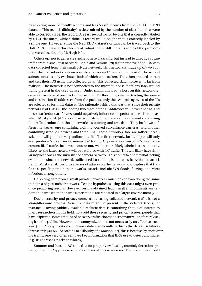
2.4. Dataset collection and generationThere is a particular pair of datasets that is widely used for machine learning-basedintrusion detection research [5, 13, 48, 74, 89], namely the DARPA 1998/1999 IntrusionDetection Evaluation Datasets [31] by Lippmann et al. [33], and its derivative KDD Cup1999 dataset [85]. It is a dataset generated by DARPA, as the name suggests, that con-sists of seven weeks of network traffic. Different versions exists, and these versions areidentified by the year they were created. DARPA claim that this generated dataset issimilar to real network traffic found inside actual Air Force bases. This network traf-fic contains benign activity of hundreds of users on thousands of UNIX hosts. Addi-tionally, this dataset contains malicious traffic produced by an assortment of differentattacks that were launched against hosts in the network. Originally there had beenlittle intrusion detection research using a single dataset shared by different researchgroups. Privacy concerns about the captured network traffic always complicate thepublication of such datasets. Also, a wide range of attacks must be successfully per-formed against different hosts with different systems. For the most part, datasets backthen had neither a wide range of attacks nor a large number of hosts. The networkin the dataset is split into two segments: the internal segment (i.e. inside the base),and the external segment (i.e. outside the base). In the internal segment, there arethree machines that serve as the victim machines, and a gateway that serves as a linkwith the rest of Air Force base PCs and workstations. Most of the hosts in the internalsegment run UNIX-based operating systems. The 1999 edition of the DARPA datasetalso contains Windows NT hosts. A Cisco router connects the inside network with theoutside. The external segment is supposed to represent the Internet. It contains twodifferent gateways: one that provides access to outside web servers, and another thatprovides outside workstations access to the network. This second gateway is wherethe attacks are launched from. Finally, the traffic sniffer is located in front of the Ciscorouter, on the outside. This placement of the sniffer means that internal network traf-fic is not captured. Only the communication between the inside and outside networksis captured. See Figure 2.1 for an illustration of the network. This private network
2.4. Dataset collection and generation 11
was used to generate network traffic that is “similar” to traffic found in real Air Forcebases. The hosts within the internal network segment ran software that generated alarge quantity of network traffic. This allowed a single host to act as if it were instead acollection of hosts, each with its own IP address. User actions such as sending email,using FTP services, or accessing other hosts via Telnet, were automated. These au-tomated user actions were performed using the same software that was used in realAir Force base networks. Examples include sendmail, ftp, and Telnet [33]. Additionalprotocols that can be found in the dataset include HTTP, IRC, DNS, and SNMP, amongothers. The timing of the usage of the different services, as well as the proportions ofall the traffic corresponding to each individual service, was based on actual Air Forcebase network usage, claim Lippmann et al [34]. Usage of synthetic data instead of ac-tual network traffic is due to security and privacy concerns. For the 1998 version of theDARPA dataset, the network traffic included 38 different types of attacks. These attacksrange from reconnaissance activities, like Nmap scans and port sweeps, to more mali-cious ones, such as Smurf [26] and Ping of Death attacks [9]. Much of the attack trafficwas present in the training data. However, many of the attack types were only placedin the test data. This was done to test the effectiveness of IDSs on not only known at-tacks, but on novel attacks as well. Some of the attacks were performed on softwarevulnerabilities that were discovered specifically for the project. The 38 types of attacksare classified into the following four groups: Denial of Service, Remote-to-Local, User-to-Root, and probes. Of these four groups, the tested IDSs were able to “generalizewell” to probes and User-to-Root attacks, but were not able to detect unseen Denial ofService and Remote-to-Local attacks accurately.
Many researchers have been using the DARPA datasets and its derivatives for theirown research projects. They do this in spite of the thorough criticisms the datasetshave received. McHugh’s 2000 paper [40] is one such example. On the datasets, hementions the claim by Lippmann et al. that the network traffic contained in the datasetsare “similar” to real Air Force base traffic, and criticizes the lack of evidence supportingthat claim, statistical or otherwise. Also, McHugh states that Lippman et al. only speakof the frequency and usage time of software utilities. The similarity of the contentof the network traffic created by the utilities is never discussed. It is only mentionedthat the network traffic is constructed using public domain and randomly generateddata sources. Furthermore, no analysis is provided as to the false positive rates of thesynthesized background data. According to McHugh [40], this type of analysis is im-portant, because in order for the synthesized traffic to be a valid substitute for realnetwork traffic, the false positive behavior of the tested IDSs should not differ signif-icantly when classifying real and synthetic network traffic. Another point raised byMcHugh is that Lippmann et al. do not discuss the data rate within their syntheticnetwork, nor any variation in this data rate over time. A quick examination of someof the DARPA dataset revealed an unrealistically low data rate, especially for a networkcontaining such a large number of hosts. Due to this low data rate, the false alarmrates would differ significantly if the IDS were tested on a noisier and more realisticnetwork. As for the attack data, McHugh criticizes the distribution of the attack traf-fic among the background traffic. Most notably, every type of attack was performedroughly the same amount of times. This creates an unrealistic scenario, according toMcHugh, since surveillance or probing activities are by far the most prevalent cause ofmalicious traffic.
Mahoney and Chan [36] are others who criticize the DARPA datasets. They do thisusing a more detailed approach than McHugh [40]. They focus on specific aspects of
12 2. Background literature
the synthetic background traffic and simulated attack traffic. Firstly, they show thatthe network traffic collected from the artificial Air Force base contains simulation arti-facts that can be utilized in order to detect attacks. To demonstrate this, they createdan IDS of very poor quality. This IDS bases its anomaly detection on a single byte ofa packet. If this specific byte was not seen during the training phase (and 60 secondshave passed without detecting an anomaly), then the packet is classified as malicious.It is clear that this IDS would be useless in a real-world scenario. In this particularcase, however, this IDS detects 45% of all attacks, with 43 false positives. This perfor-mance is comparable with the best-performing systems in the original DARPA datasetevaluation. Mahoney and Chan collected network traffic from a university departmen-tal server and mixed this captured traffic into the DARPA dataset. After training andtesting on this newly created dataset, the IDS was barely able to detect any attack atall. Additionally, the false positive rate increased significantly. They also comparedthe synthetic background data to real network traffic they collected from a universityserver. This comparison yielded several findings. For instance, many of the DARPApackets have no IP, TCP, UDP, or ICMP checksums. Also, they found a lack of varietyin many of the DARPA packet fields. The packets’ TTL fields were set only to nine val-ues out of the possible 256 values. The real network traffic, on the other hand, had177 different values. Furthermore, compared to the DARPA dataset, the real networktraffic had much more variety in the types of HTTP, SMTP, and SSH requests. Usingthese values as part of an anomaly detection rule would result in a high false positiverate, since the values are much less predictable in real-world traffic. This is especiallyevident given the low-quality simulation of several attacks. Attacks such as dosnuke,neptune, and queso [33], among others, use only two different TTL values. ICMP pack-ets in the smurf [26] attack contain checksum errors. Detecting these attacks usingthese attributes might increase the performance of the IDS when operating on theDARPA datasets, but such an IDS would be worthless in the real world. Despite themany shortcomings of the DARPA datasets, Mahoney and Chan considered it to be themost sophisticated dataset that was publicly available. To alleviate the dataset’s inher-ent problems, they propose mixing real traffic into the simulated traffic. Though inthis case, it would be important that the real traffic be transformed in such a way thatwould make the real and simulated traffic indistinguishable to an IDS.
Tavallaee et al. [80] performed an analysis on the KDD Cup 1999 dataset. In thisanalysis, they found two significant issues that plague the dataset. These issues affectthe performance of the anomaly detection systems, which in turn results in an inad-equate evaluation of said systems by researchers. The first issue is the vast amount ofredundant records in the KDD Cup 1999 dataset. Training a classifier on this datasetcause it to be biased towards these redundant (frequently-occurring) records, whichmakes the classifier much less likely to learn from records that occur less frequently.Furthermore, these duplicate records in the test set will cause the classifier to presenta much higher detection rate for these specific records than for less frequent records.Tavallaee et al. solved this issue by removing all duplicate records and keeping only asingle instance of each record. They also found that simply using accuracy, detection,and false positive rates for evaluation when using the KDD Cup 1999 dataset is an un-suitable approach for evaluating an anomaly detection system. They discovered thisby learning 21 different classifiers on random subsets of the dataset, and then havingthese classifiers label all the records in the training and test sets. All 21 classifiers wereable to correctly label 98% of the training set and 87% of the test set. To address thissecond issue, the NSL-KDD dataset is made more “challenging”. Tavallaee et al. do this
2.4. Dataset collection and generation 13
by selecting more “difficult” records and less “easy” records from the KDD Cup 1999dataset. This record “difficulty” is determined by the number of classifiers that wereable to correctly label the record. An easy record would be one that is correctly labeledby all 21 classifiers, while a difficult record would be one that is correctly labeled bya single one. However, since the NSL-KDD dataset’s origins can be traced back to theDARPA 1998 dataset, Tavallaee et al. admit that it still contains some of the problemsthat were described by McHugh [40].
Others opt not to generate synthetic network traffic, but instead to directly capturetraffic from a small test network. Labib and Vemuri [29] test their developed IDS withdata collected from their small private network. This network is made up of two sub-nets. The first subnet contains a single attacker and “tens of other hosts”. The secondsubnet contains only two hosts, both of which are attackers. They then proceed to trainand test their IDS using the collected data. This collected data, however, is far fromrealistic. The network is not connected to the Internet, nor is there any backgroundtraffic present in the used dataset. Under minimum load, a host on this network re-ceives an average of one packet per second. Furthermore, when extracting the sourceand destination IP addresses from the packets, only the two trailing bytes of the IPsare selected to form the dataset. The rationale behind this was that, since their privatenetwork is of Class C, the leading two bytes of the IP addresses will never change, andthese two “redundant” bytes would negatively influence the performance of their clas-sifier. Mirsky et al. [47] also chose to construct their own sample networks and usingthe traffic produced in those networks as training and test data. They built two dif-ferent networks: one containing eight networked surveillance cameras, and anothercontaining nine IoT devices and three PCs. These networks, too, are rather unreal-istic, and will produce very uniform traffic. The first network, for example, will onlyever produce “surveillance camera-like” traffic. Any deviation from this “surveillancecamera-like” traffic, be it malicious or not, will be more likely labeled as an anomaly.Likewise, the latter network will be saturated with IoT traffic. This will likely have simi-lar implications as the surveillance camera network. This points to a somewhat lackingevaluation, since the network traffic used for training is not realistic. As for the attacktraffic, Mirsky et al. perform a series of attacks on the networks and capture that traf-fic at a specific point in the networks. Attacks include SYN floods, fuzzing, and Miraiinfection, among others.
Collecting data from a small private network is much easier than doing the samething in a bigger, noisier network. Testing hypotheses using this data might even pro-duce promising results. However, results obtained from small environments are sel-dom the same when the same experiments are repeated in a larger environment [73].
Due to security and privacy concerns, releasing collected network traffic is not astraightforward process. Sensitive data might be present in the network traces, forinstance. Having publicly available realistic data is something that is of interest tomany researchers in this field. To avoid these security and privacy issues, people thathave captured some amount of network traffic choose to anonymize it before releas-ing it to the public. However, this anonymization is not necessarily an effective mea-sure [11]. Anonymization of network data significantly reduces the data’s usefulnessfor research [30, 56]. According to Killourhy and Maxion [27], this is because by anonymiz-ing traffic, one very often removes key information that IDSs use to detect anomalies(e.g. IP addresses, packet payloads).
Sommer and Paxson [73] state that for properly evaluating anomaly detection sys-tems, obtaining “appropriate data” is the most important issue. The researcher should
14 2. Background literature
strive to acquire a dataset that contains real network traffic. This network traffic shouldalso be collected from network that is as large as possible. If possible, different datasetscollected from different networks should be used. They state that working with actualtraffic increases the quality of research, since one can immediately observe the perfor-mance of the studied IDS in a real-world scenario.
Figure 2.1: Diagram of the network in the DARPA datasets [33]
2.5. SummaryMuch research has been done in the field of intrusion detection. Many different ma-chine learning techniques have been applied to this problem, with many researchersclaiming to have created highly effective IDSs. These “highly effective” IDSs are de-signed and evaluated using methodologies and datasets that have been heavily crit-icized by others. For instance, most of the papers discussed in Section 2.2 use someflawed dataset, as the papers by McHugh et al. [40] and Mahoney and Chan [36] havedemonstrated. The rest use data from small, private networks, which is inadvisable,according to Sommer and Paxson [73].
There seems to be large disconnect between these two groups of researchers. Onegroup criticizes current methodologies and suggests more suitable alternatives, whilethe other group never seems to adjust their approach to anomaly detection researchin order to improve the quality of their work.
None of this research has ever been revisited in order to test how the same method-ologies and technologies will perform in a real-world scenario, with real network traf-fic, as Sommer and Paxson suggest [73]. This is unfortunate, since much of this re-search may contain erroneous results and conclusions. Future research is then builton top of these possibly erroneous conclusions, as many researchers will not doubt thevalidity of published research articles. It is therefore in the interest of the entire field ofanomaly detection to verify the findings of such published research.
3Case study
From the background literature presented in Chapter 2, we see many different ap-proaches and methods being developed to resolve a common task, namely automaticintrusion detection. However, many of these methods use data that is flawed [36, 40]for not only the training of the classifiers, but the evaluation as well. The fact that theseinadequate methodologies and data are used for the realization of academic researchraises questions about the validity of said research.
It is therefore interesting to see whether these approaches are able to hold theirown when correctly tested in a real-world environment. By using real-world networktraffic data, we will be able to appropriately evaluate the developed approaches, as wellas the validity of the authors’ conclusions.
3.1. IDS selectionThe first thing that is necessary for this research is an IDS that we can study. Section 2.2lists a number of IDSs that were developed over the years. We will select one of theseIDSs for this project. This choice is made with two factors in mind: the age of thesystem, and its ease of use.
We prefer the IDS to be as recent as possible. Using recent research ensures thatthe techniques used are up to date with current developments in the field of anomalydetection. The two most recent works discussed in Chapter 2 are the systems proposedby Shone et al. [70] and Mirsky et al. [47]. Both published their research early 2018.Coincidentally, both use autoencoder-based approaches for the design of their IDS.
The final selection will therefore be based on each system’s ease of use. Due tothe time constraints set upon this project, we very much favor a system that is easyto set up and easy to use. The system by Mirsky et al. [47] clearly has the advantageover the system by Shone et al. [70] Shone et al. have not made their system publiclyavailable, so trying to obtain it would be unnecessarily time-consuming. On the otherhand, the IDS by Mirsky et al. is open-source, and they have made it publicly availableon GitHub [44]. The public availability of the source code makes it a straightforwardprocess to install the system on our machines. Furthermore, this system also takes itsinput data in raw pcap format, meaning that newly captured network traces can easilybe fed into the system without the need for any data transformation or feature extrac-tion. Thus, the IDS chosen for this research is the Kitsune IDS by Mirsky et al. [47].
15

16 3. Case study
Figure 3.1: Architecture of Kitsune [47]
3.2. KitsuneThe Kitsune system is not simply a classifier, but includes an entire framework of func-tionality. The system uses autoencoders to learn the “normal” behavior of the networkin order to, later on, detect deviations from this “normal” behavior.
An autoencoder is a type of artificial neural network that is trained in an unsuper-vised manner to create a representation of its input [32]. Explained simply, an autoen-coder encodes the data it receives as input as an object of lower dimensionality, afterwhich it tries to reconstruct the higher-dimensional object as accurately as possible.
Its functionality comprises the following elements:
1. Feature Extractor;
2. Feature Mapper; and
3. Anomaly Detector.
See Figure 3.1 for an illustration of Kitsune’s architecture.
3.2.1. ComponentsThis section will discuss the aforementioned components of Kitsune, as well as someof the relevant technical details.
Feature Extractor
Kitsune does not directly operate on raw packet data. Instead, as its name sug-gests, the Feature Extractor component extracts a collection of features from ev-ery captured packet. Packets are parsed and certain information is extractedfrom them. Specifically, the following fields are selected:
– IP version (IPv4/IPv6);
– packet timestamp;
– frame length;
– source and destination IP;
– source and destination MAC address; and
– transport, internet, or link layer protocol [79].
It is from these fields that the eventual features are actually constructed from.
Mirsky et al. emphasize the importance of analyzing the temporal features ofnetwork traffic to find anomalies and possible intrusions. Instead of using packetwindows to compute these statistics, Kitsune uses packet timestamps to createdamped windows, using a technique that Mirsky et al. call Damped Incremental

3.2. Kitsune 17
Statistics. They claim using a conventional window will not scale due to memoryusage, which is one of the reasons for the usage of their damped windows. Foreach packet that arrives, the previously mentioned fields are retrieved. Thesefields are then used to update the statistics in the damped window.
The goal of damped windows is to maintain the temporal statistics of a collec-tion of packets within a given time window, but have the weight of older valuesdecrease as time goes on. Temporal statistics are computed for five differenttime windows λ: 100ms, 500ms, 1.5s, 10s, and 1min (λ = 5,3,1,0.1,0.01). Forevery one of these time windows, Kitsune maintains a collection of incrementalstatistics tuples for each of the following:
– every source MAC-IP address (denoted SrcMAC-IP 1);
– every source and destination IP address pair (denoted SrcIP);
– every connection between a source IP and destination IP (denoted Chan-nel); and
– every connection between a source IP-port pair and destination IP-portpair (denoted Socket);
For all records except the SrcIP records, Kitsune extracts from packets both thepacket size and timestamp. The purpose of the SrcIP records is to capture jit-ter behavior between different hosts, and therefore only extracts timestamps.The tuples corresponding to SrcMAC-IP and SrcIP are used to compute one-dimensional (1D) statistics. The tuples corresponding to Channel and Socketare used to compute two-dimensional (2D) statistics. This naming (1D and 2D)refers to the number of tuples involved in the statistics computations: the 1Dstatistics involve a single one of these tuples, while the 2D statistics are com-puted using two different tuples. The tuples are defined as
I Si ,λ← (w,LS,SS,SRi j ,Tl ast ),
where λ is the time window, w is the weight, LS is the linear sum of the packetsizes, SS is the sum of the squares of the packet sizes, SRi j is the sum of resid-ual products between the tuples I Si ,λ and I S j ,λ, and Tl ast is the timestamp ofthe most recently received packet that corresponds to the given tuple. SRi j usesdata from two different tuples, and is only present in the tuples used for 2D com-putations: Channel and Socket.
Kitsune creates or fetches a tuple for every packet that it receives. It then usesthese tuples to compute a total of 23 statistics to capture the behavior of thenetwork for each of the given time windows. Thus, a total of 115 features areextracted. See Figure 3.2 for the full list of features extracted from the tuples.
It is important to note that the usage of 2D statistics makes Kitsune detectioncontext-dependent. By this, we mean that previous behavior between two hosts,if there is any, is taken into account when evaluating traffic. Therefore, it matterswhether traffic is evaluated within the context of other network traffic or out ofcontext. For example, say there is a malicious host that had previously interactedwith the network in a strictly benign manner. If this host suddenly launches anattack, Kitsune will evaluate these malicious packets differently than in a situa-tion where the malicious host had not previously interacted with the network atall.
1notation taken from Mirsky et al.[47]

18 3. Case study
Figure 3.2: Statistics computed by Kitsune using the incremental statistics tuples [47]
Feature Mapper
The features that are extracted from the network traffic are passed to the FeatureMapper. The Feature Mapper then processes these features in order to producethe input for the Anomaly Detector’s ensemble of autoencoders.
Firstly, the features that are given as input are clustered together using correla-tion between features as the distance between them, which they define as
dcor (u, v) = 1− (u −u) · (v − v)
‖(u −u)‖2‖(v − v)‖2,
where u is the mean of the elements in vector u, and u ·v is the dot product [47].
Out of the 115 features extracted, every cluster will be constructed in such a waythat it contains at most m features, where m is a user-defined parameter. So,each autoencoder will have a maximum of m inputs. This parameter has aneffect on the complexity of the autoencoder ensemble, and therefore also onthe speed and performance of the system as a whole. Mirsky et al. state thata smaller m will “usually” make Kitsune perform better than a higher value ofm, although processing speed will decrease significantly [47]. This makes sense,since a smaller m will lead to a larger amount of clusters, which which will inturn lead to an increase in complexity.
The output of this component is a list of these feature clusters.
Anomaly Detector
The Anomaly Detector is made up of two layers of autoencoders: the EnsembleLayer, and the Output Layer. The Ensemble Layer takes the list of feature clustersas input, while the Output Layer takes the output of the Ensemble Layer as input.
Each autoencoder in the Ensemble Layer will be assigned a single cluster of fea-tures to process. The features are mapped to a subspace and then reconstructedby the autoencoder. After the mapping and reconstruction phases, the root-mean-square error (RMSE) is computed between the original features that werethe inputs of the autoencoders and the reconstructed features. A lower RMSEindicates an accurate reconstruction of the input features, which is the objectiveof the autoencoders. All the RMSE values from the Ensemble Layer are collected,and provided as input to the Output Layer.
3.2. Kitsune 19
The Output Layer is a single autoencoder that has the same amount of inputsas the Ensemble Layer has autoencoders. Every RMSE value from the EnsembleLayer is fed into the Output Layer. Initially, this final autoencoder is trained onthe RMSE values that are computed with normal network traffic. When actu-ally in operation, the Output Layer tries to reconstruct the original RMSE values.It then computes takes the original RMSEs and the reconstructed RMSEs andcomputes one final RMSE value, which will serve as the packet’s anomaly score.
The previous was a brief overview of Kitsune’s inner workings. For a more de-tailed description of the mathematics and algorithms behind Kitsune, see the paperby Mirsky et al. [47].
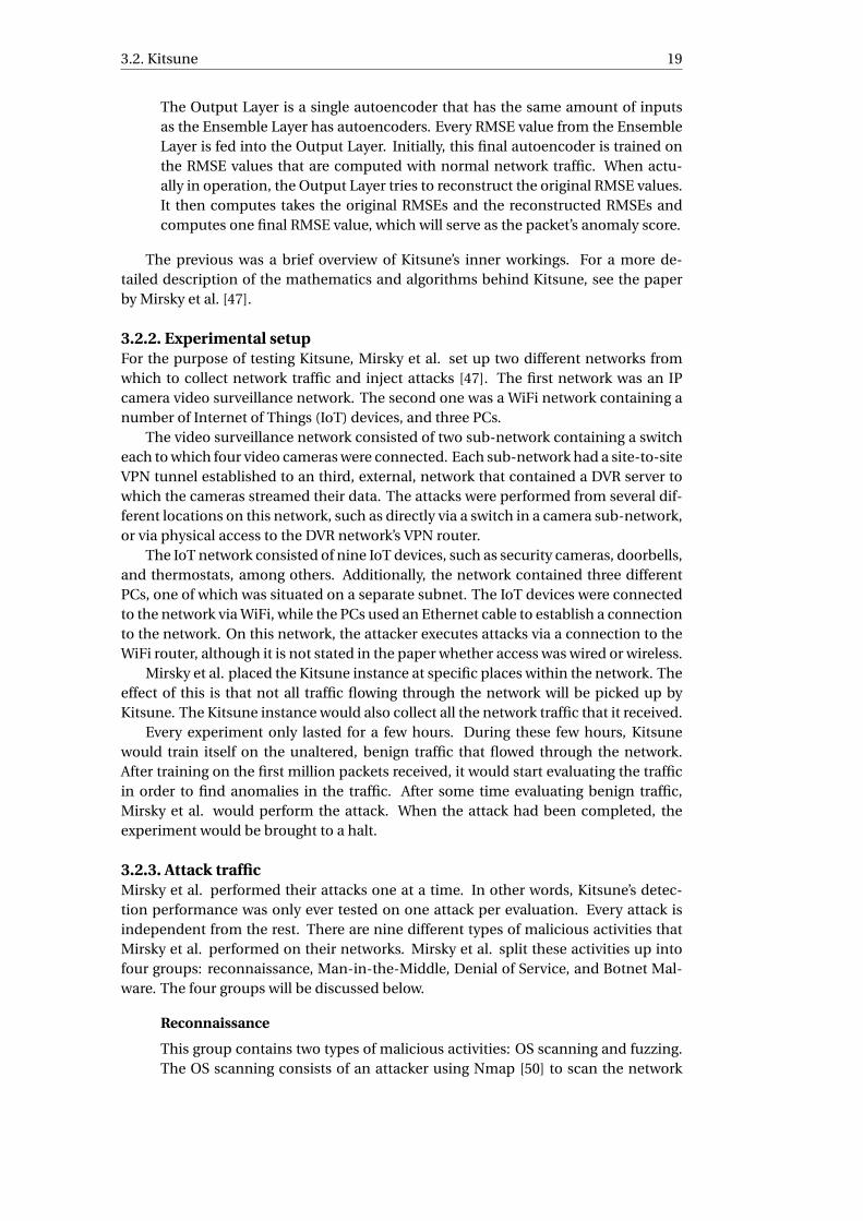
3.2.2. Experimental setupFor the purpose of testing Kitsune, Mirsky et al. set up two different networks fromwhich to collect network traffic and inject attacks [47]. The first network was an IPcamera video surveillance network. The second one was a WiFi network containing anumber of Internet of Things (IoT) devices, and three PCs.
The video surveillance network consisted of two sub-network containing a switcheach to which four video cameras were connected. Each sub-network had a site-to-siteVPN tunnel established to an third, external, network that contained a DVR server towhich the cameras streamed their data. The attacks were performed from several dif-ferent locations on this network, such as directly via a switch in a camera sub-network,or via physical access to the DVR network’s VPN router.
The IoT network consisted of nine IoT devices, such as security cameras, doorbells,and thermostats, among others. Additionally, the network contained three differentPCs, one of which was situated on a separate subnet. The IoT devices were connectedto the network via WiFi, while the PCs used an Ethernet cable to establish a connectionto the network. On this network, the attacker executes attacks via a connection to theWiFi router, although it is not stated in the paper whether access was wired or wireless.
Mirsky et al. placed the Kitsune instance at specific places within the network. Theeffect of this is that not all traffic flowing through the network will be picked up byKitsune. The Kitsune instance would also collect all the network traffic that it received.
Every experiment only lasted for a few hours. During these few hours, Kitsunewould train itself on the unaltered, benign traffic that flowed through the network.After training on the first million packets received, it would start evaluating the trafficin order to find anomalies in the traffic. After some time evaluating benign traffic,Mirsky et al. would perform the attack. When the attack had been completed, theexperiment would be brought to a halt.
3.2.3. Attack trafficMirsky et al. performed their attacks one at a time. In other words, Kitsune’s detec-tion performance was only ever tested on one attack per evaluation. Every attack isindependent from the rest. There are nine different types of malicious activities thatMirsky et al. performed on their networks. Mirsky et al. split these activities up intofour groups: reconnaissance, Man-in-the-Middle, Denial of Service, and Botnet Mal-ware. The four groups will be discussed below.
Reconnaissance
This group contains two types of malicious activities: OS scanning and fuzzing.The OS scanning consists of an attacker using Nmap [50] to scan the network
20 3. Case study
and its hosts and operating system in order to find any possible vulnerabilities.
The fuzzing attack uses SFuzz [10] to probe the surveillance camera’s web servers.It sends a collection of malformed CGI commands to the web servers in hopesof triggering an error and find a vulnerability.
Man-in-the-Middle
These attacks are a special case. As mentioned in Section 3.2.2, the Kitsune in-stance would not receive all the network traffic that flowed through the network.Mirsky et al. state that, although the actual malicious traffic would not be seenby the Kitsune instance, statistical changes in the network’s behavior would bepicked up by Kitsune due to its usage of incremental statistics. They state thatnetwork behavior caused by Man-in-the-Middle attacks, such as packet jitter,can be detected this way.
There are three types of Man-in-the-Middle attacks that were performed on thenetworks. The first is video injection. Since the surveillance cameras maintaina constant stream of video traffic to the DVR server, it is possible for a maliciousactor with access to the network to access this traffic. In this attack, Mirsky et al.inject a recorded video clip into a camera’s live video stream.
The second attack is an ARP poisoning attack. They poison ARP caches in orderto intercept the network traffic between a surveillance camera and the DVR.
The third is the usage of an active wiretap. It is performed by installing a networkbridge on an exposed network cable. This allows the attacker to intercept allnetwork traffic flowing across the network bridge.
Denial of Service
Mirsky et al. perform three types of DoS attacks against their network, the first ofwhich is an SSDP flood. The surveillance cameras use SSDP to advertise them-selves on the network. This can be exploited by attackers who want to overload ahost. The attacker sends the cameras an SSDP request with the IP address of theDVR as a spoofed address. Once received, the cameras “reply” to the DVR with amuch larger SSDP response. This overloads the DVR server.
Second is a SYN flood. Mirsky et al. overload a camera’s web server by sendingit a large number of SYN packets. The result of this attack is the disabling of thecamera’s live video stream.
Lastly is an SSL renegotiation attack. Using the RSA cryptosystem, decryptiontakes significantly longer than encryption. This is because the private exponentis computed as the modular multiplicative inverse of the pubic exponent, there-fore making it much larger than the public exponent [88]. Due to this imbalancein processing speeds, an attacker can flood an SSL service with SSL renegotia-tion requests and disable it by forcing it to perform a huge amount of expensivedecryptions. Mirsky et al. perform this attack on one of the cameras, which dis-ables its live video stream.
Botnet Malware
Mirsky et al. perform this attack not on their surveillance camera network, buton their IoT network. A malicious actor connects to the network’s WiFi accesspoint. He then scans the network for available Telnet services. When one ofthese services is found on an IoT device, the attacker connects to it using default
3.2. Kitsune 21
admin credentials and installs on it the Mirai malware. The infected IoT devicethen starts scanning the network using ARP requests in order to find more livehosts to infect.
3.2.4. EvaluationAs discussed in Section 3.2.1 of this chapter, the final output of Kitsune is an RMSEvalue that serves as an anomaly score for the currently processed packet. The greaterthis RMSE value, the greater the anomaly [47]. A RMSE by itself, however, is not suf-ficient to classify traffic as anomalous. A threshold value needs to be chosen first.Any packet that receives a final RMSE score below this threshold is considered benign.Packets receiving scores above the threshold are classified as anomalous.
Naturally, the choice of threshold value will determine the accuracy of classifica-tion, and hence the overall performance of the classifier itself. Therefore, it is impor-tant that this threshold is not chosen in an arbitrary manner. A way of choosing thisthreshold is to minimize the number of false positives generated by the classifier, sinceintrusion detection systems become practically unusable with even a minute false pos-itive rate [3]. This is the approach that is taken by Mirsky et al. for determining theirthreshold value [47].
For every attack, they select two different thresholds that would give them fixedfalse positive rates of 0 and 0.001 when classifying the benign traffic. We will referto these thresholds as F PR = 0 and F PR = 0.001, respectively. After selecting thesetwo thresholds, the portion of network traffic containing the attack itself is classified.Applying the F PR = 0 and F PR = 0.001 thresholds to the malicious traffic, Mirskyet al. compute two statistics for each threshold (four in total): the true positive rate(TPR) and false negative rate (FNR). In addition to the TPR and FNR, Mirsky et al. usetwo ROC curve [83] statistics: Area Under the Curve (AUC) [17], and Equal Error Rate(EER) [69]. These statistics are computed, not only for Kistune, but for other IDSs andalgorithms, such as Suricata [76], Isolation Forest [35] and pcStream [46]. Kitsune’soverall performance is then determined by comparing it to the performance of theother algorithms on the same attacks.

4Data collection and processing
Usage of inadequate data for the development of IDSs has been highlighted in Chap-ter 2. As stated by Sommer and Paxson [73], one should aim at acquiring a dataset thatcontains real network traffic from an environment that is as large as one can get theirhands on. This is an important aspect of data collection, because it cannot be assumedthat analysis of small environments will yield the same results when such an analysis isperformed on larger and more realistic environments [72]. Performing one’s researchon real network traffic, as opposed to pre-collected data or data collected from an arti-ficial network, improves the quality of the research and its results, since the evaluationof the system will demonstrate its performance in a real-world scenario [73].
4.1. Obtaining appropriate dataFor this research, we will not use pre-collected datasets, such as the DARPA 1998/1999 [31]or KDD Cup 1999 datasets [85]. Neither will we be collecting network traffic from smallexperiment networks, as Labib and Vemuri [29], and Mirsky et al. [47] have done. In-stead, we will follow the recommendations by Sommer and Paxson [73]. They statethat it is important to a research project that datasets be collected from a real-worldenvironment.
We must find and obtain access to as large a network as we can. If this networkbelongs to a third party, agreements need to be made about proper storage and usageof any captured network traffic. Once the agreements have been made and networkaccess has been provided, we will start capturing network traffic. Several weeks ofnetwork traffic will be collected in order to have enough variety in the eventual networktraces. This variety in the traces can include many unique IP addresses, usage of manydifferent protocols, and variety in packet sizes, among many others. Special care needsto be taken of the possible privacy concerns that may arise. In any case that involvessensitive data, measures need to be taken in order to secure this data. If necessary, thissensitive data should be anonymized before being processed.
As stated by Sommer and Paxson [73], obtaining ground-truth data is imperativefor proper IDS evaluation. Without knowledge of the network that is used, it is impos-sible to obtain this ground-truth. Therefore, cooperation between us and the networkadministrator is necessary. The network administrator will need to provide a thor-ough description of the network. This includes the hosts, which services are runningon which ports, and how the hosts communicate between themselves and with exter-nal hosts on the Internet. When we have received the description of the network, we
23
24 4. Data collection and processing
will begin filtering the captured network. The goal is to obtain ground-truth data byfiltering network traffic so that we end up with two sets of network traffic for whichwe know with absolute certainty that one contains only normal traffic and the othercontains only illegitimate or malicious traffic.
The filtering will be performed by creating a static rule-set from the provided net-work description. It is likely that this network description will be incomplete, meaningthat the rule-set created from the description will be incomplete as well. Filtering thenetwork traces using this rule-set will split the data into three categories: legitimatetraffic, illegitimate traffic, and unclassified (i.e. traffic for which no rule currently ex-ists). The next part of the filtering must be an iterative process. Of the unclassifiedtraffic, we will select a subset and discuss this traffic with the network administrator.The network administrator will label this traffic as legitimate or illegitimate. We willthen update the network description and the rule-set, and, once again, filter the net-work traces. This process is repeated until the unclassified traffic disappears and therule-set is able to filter all of the captured network traffic into either the legitimateor illegitimate category. In the case that ground-truth cannot be established about aspecific type of network traffic, it will be removed from the dataset. Ground-truth isessential for anomaly detection datasets, so data of which we are uncertain cannot beincluded in our datasets.
4.2. Network descriptionThe data that will be used in this research is taken from a real-world network. Thissection will describe the layout of this network, as well as the components that it ismade out of.
The services provided by this network are used by a multitude of users from differ-ent places all over the world. While itself a relatively small network compared to largeorganizations, many types of traffic that are also found in such large organizations,such as mail, web, and DNS traffic. The presence of these different types of networktraffic makes this used network a much more realistic one than the artificial networkcreated by Mirsky et al. for their paper [47], since that network mostly consisted out ofIP cameras that output video traffic.
In addition to using IPv4, this network also accepts the newer IPv6 and can use it tocommunicate. All components of the network have both an IPv4 address and an IPv6,with the only exception being the private DNS server. This private DNS server is onlyassigned an IPv4 address.
The network used in this research contains (i) a gateway, (ii) a mail server, (iii) aweb server, (iv) a public DNS server, (v) a private DNS server, (vi) a shell access server,and (vii) a web server requiring authentication.
While every component on the network is a separate and independent unit, in ac-tuality, they are all virtual machines (VM) running on the same physical server. Thegateway VM is the only component that is directly connected to the Internet. Its jobin the network is to provide the remaining virtual machines with Internet access, andto allow for communication between said virtual machines. It does this by means ofa virtual bridge. This virtual bridge is set up on the gateway VM, and is configured tocontain all of the other virtual machines as interfaces. See Figure 4.1 for a diagram ofthe network.
All virtual machines on this server are running OpenBSD 6.3 [52] as operating sys-tem. OS distribution updates are downloaded from an OpenBSD mirror1. An SSH ser-
1https://ftp.halifax.rwth-aachen.de/
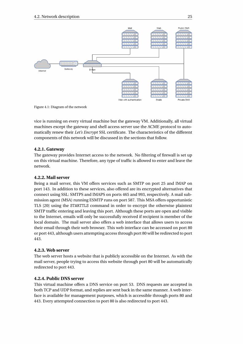
4.2. Network description 25
Figure 4.1: Diagram of the network
vice is running on every virtual machine but the gateway VM. Additionally, all virtualmachines except the gateway and shell access server use the ACME protocol to auto-matically renew their Let’s Encrypt SSL certificate. The characteristics of the differentcomponents of this network will be discussed in the sections that follow.
4.2.1. GatewayThe gateway provides Internet access to the network. No filtering of firewall is set upon this virtual machine. Therefore, any type of traffic is allowed to enter and leave thenetwork.
4.2.2. Mail serverBeing a mail server, this VM offers services such as SMTP on port 25 and IMAP onport 143. In addition to these services, also offered are its encrypted alternatives thatconnect using SSL: SMTPS and IMAPS on ports 465 and 993, respectively. A mail sub-mission agent (MSA) running ESMTP runs on port 587. This MSA offers opportunisticTLS [20] using the STARTTLS command in order to encrypt the otherwise plaintextSMTP traffic entering and leaving this port. Although these ports are open and visibleto the Internet, emails will only be successfully received if recipient is member of thelocal domain. The mail server also offers a web interface that allows users to accesstheir email through their web browser. This web interface can be accessed on port 80or port 443, although users attempting access through port 80 will be redirected to port443.
4.2.3. Web serverThe web server hosts a website that is publicly accessible on the Internet. As with themail server, people trying to access this website through port 80 will be automaticallyredirected to port 443.
4.2.4. Public DNS serverThis virtual machine offers a DNS service on port 53. DNS requests are accepted inboth TCP and UDP format, and replies are sent back in the same manner. A web inter-face is available for management purposes, which is accessible through ports 80 and443. Every attempted connection to port 80 is also redirected to port 443.
26 4. Data collection and processing
4.2.5. Private DNS serverThe private DNS server provides the same services and functionality that the publicDNS server does. The only difference is that DNS requests to this server originate onlyfrom within the local network. Outside access to this server is prohibited.
4.2.6. Shell access serverThe only service this server itself provides is SSH on port 22. This port is accessiblefrom the Internet, although only authorized users are allowed to utilize it. The usersthemselves then have the ability to run or access services that produce other networktraffic, such as ICQ, XMPP, and IRC.
4.2.7. Web server with authenticationThis virtual machine is also a web server. In contrast to the public web server, how-ever, this server uses HTTP Basic authentication in order to grant users access to theweb page. All HTTP requests to port 80 are redirected to port 443. This is necessaryfor confidentiality, since HTTP Basic authentication does not encrypt user credentialsbefore sending them to the web server.
4.3. Capturing network trafficFor the purpose of collecting the network traffic necessary for this research, we madeuse of tcpdump, which is a packet capture and analysis tool [81]. A tcpdump instancewas set up on the gateway VM to capture all the traffic that passes the virtual networkbridge. This includes incoming and outgoing Internet traffic, as well as internal com-munication between the virtual machines themselves within the network.
When writing network traffic to a file, tcpdump writes raw packets straight to disk [39].These packet captures are saved to a pcap file, which contains the captured sequenceof raw packets. This allows the tcpdump instance to run as fast as possible in order tominimize the amount of dropped packets [39].
This tcpdump instance ran uninterrupted for a period of seven weeks, or 49 days.During this time, a total of 33.7 GB of traffic was captured, containing approximately240000 unique IP addresses. Per day, the average packet capture file is around 690 MBin size and contains 12170 unique IP addresses.
4.3.1. SanitationThis is a real-world network with actual users. Given the possibility that the capturednetwork traces contain the users’ sensitive data, we need to take their privacy concernsinto consideration. This means that the captured data must be sanitized in order toremove all of the potentially sensitive information.
This network contains two servers that require network traffic sanitation. Theseare the mail server and the shell access server.
The mail server makes use of SMTP on port 25 for sending emails. Plain SMTP doesnot make use of encryption. Hence, capturing this traffic will also capture the contentsof the users’ emails as plaintext. In order to prevent privacy issues, any packet with port25 as either source or destination port is stripped of its TCP payload. The result of thissanitation is that all SMTP packets are transformed into empty TCP packets, meaningTCP packets with no payload.
The shell access server allows users to set up their own messaging services or con-nect to external messaging services. These messaging services include ICQ, XMPP,and IRC. Network traffic created by these messaging services are not necessarily en-
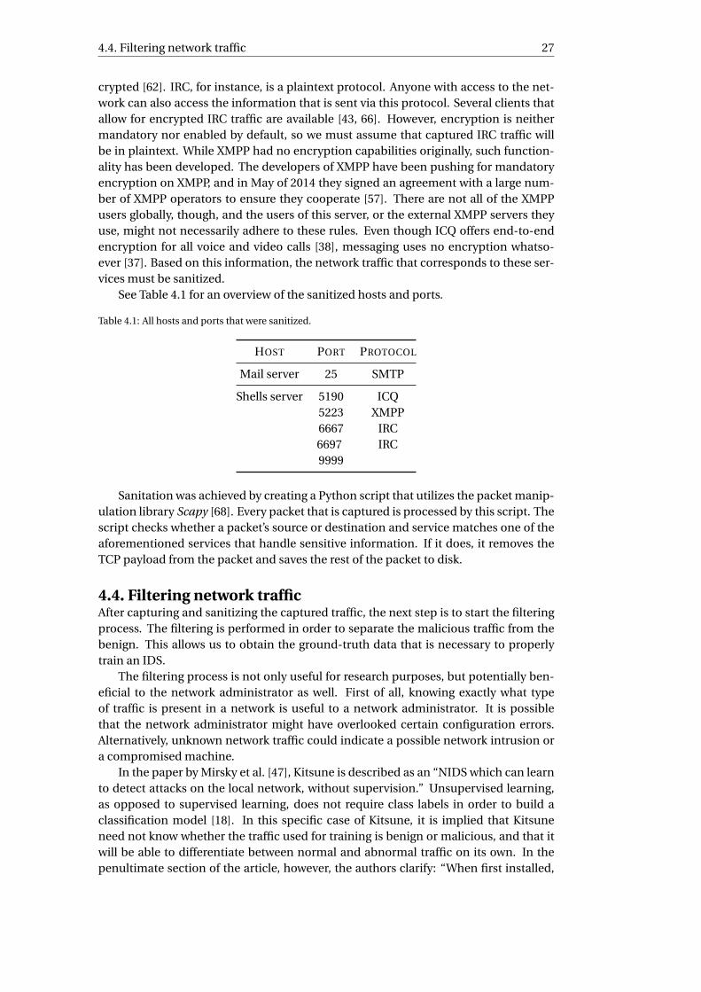
4.4. Filtering network traffic 27
crypted [62]. IRC, for instance, is a plaintext protocol. Anyone with access to the net-work can also access the information that is sent via this protocol. Several clients thatallow for encrypted IRC traffic are available [43, 66]. However, encryption is neithermandatory nor enabled by default, so we must assume that captured IRC traffic willbe in plaintext. While XMPP had no encryption capabilities originally, such function-ality has been developed. The developers of XMPP have been pushing for mandatoryencryption on XMPP, and in May of 2014 they signed an agreement with a large num-ber of XMPP operators to ensure they cooperate [57]. There are not all of the XMPPusers globally, though, and the users of this server, or the external XMPP servers theyuse, might not necessarily adhere to these rules. Even though ICQ offers end-to-endencryption for all voice and video calls [38], messaging uses no encryption whatso-ever [37]. Based on this information, the network traffic that corresponds to these ser-vices must be sanitized.
See Table 4.1 for an overview of the sanitized hosts and ports.
Table 4.1: All hosts and ports that were sanitized.
HOST PORT PROTOCOL
Mail server 25 SMTP
Shells server 5190 ICQ5223 XMPP6667 IRC6697 IRC9999
Sanitation was achieved by creating a Python script that utilizes the packet manip-ulation library Scapy [68]. Every packet that is captured is processed by this script. Thescript checks whether a packet’s source or destination and service matches one of theaforementioned services that handle sensitive information. If it does, it removes theTCP payload from the packet and saves the rest of the packet to disk.
4.4. Filtering network trafficAfter capturing and sanitizing the captured traffic, the next step is to start the filteringprocess. The filtering is performed in order to separate the malicious traffic from thebenign. This allows us to obtain the ground-truth data that is necessary to properlytrain an IDS.
The filtering process is not only useful for research purposes, but potentially ben-eficial to the network administrator as well. First of all, knowing exactly what typeof traffic is present in a network is useful to a network administrator. It is possiblethat the network administrator might have overlooked certain configuration errors.Alternatively, unknown network traffic could indicate a possible network intrusion ora compromised machine.
In the paper by Mirsky et al. [47], Kitsune is described as an “NIDS which can learnto detect attacks on the local network, without supervision.” Unsupervised learning,as opposed to supervised learning, does not require class labels in order to build aclassification model [18]. In this specific case of Kitsune, it is implied that Kitsuneneed not know whether the traffic used for training is benign or malicious, and that itwill be able to differentiate between normal and abnormal traffic on its own. In thepenultimate section of the article, however, the authors clarify: “When first installed,

28 4. Data collection and processing
Kitsune assumes that all traffic is benign while in train-mode.” Due to this, any ma-licious actors already present in the network will be able to circumvent Kitsune’s at-tempts at detection. Technically, Kitsune is an unsupervised system due to its usageof autoencoders [32] for its learning and classification process, which do not need ex-plicit labeling of data. In practicality, however, training on just normal data suggeststhat any candidate data that will be used for training must first be split up into be-nign and malicious traffic before being fed into the system. This is especially the casein the current Bring Your Own Device [6] era. People bring their own devices to theworkplace and use them to access the company network. In turn, these devices bringwith them a large collection of software that produces lots of new network traffic thatwould otherwise never be seen in the company network. Much of the traffic within acompany network will undoubtedly be benign, but one cannot say with certainty thatall of the network traffic is benign without performing some sort of analysis on saidnetwork traffic. Consequently, any real-world network traffic must be analyzed andfiltered before being used as training data.
The objective of this research is to test Kitsune’s classification performance on areal-world network that is noisier and contains a larger variety of types of networktraffic. Additionally, for anomaly detection research, it is imperative to obtain reli-able ground-truth data [73]. Therefore, the traffic that is captured cannot simply beused immediately to train a classifier. The traffic collected from this network must befiltered in order to train Kitsune on ground-truth and completely benign traffic. Anypresence of malicious or unwanted traffic in the training data will influence the classi-fier’s performance.
A Python script was created to perform the filtering process. The script utilizestcpdump’s filter rule functionality. This allows the user to extract a specific portion ofnetwork traffic from either a real-time network traffic stream, or a pcap file containingpreviously collected traffic. This script carries out a number of tasks in order to extractground-truth benign traffic.
Certain services offered by the network require authentication before usage is pos-sible. Therefore, we cannot assume that all network traffic corresponding to this ser-vice is benign. See Table 4.2 for the full list of these services. Access to these services islogged, and these logs enable us to differentiate between benign access and unwantedor malicious connection attempts. The IP addresses that attempt to access the servicesare extracted from the logs and separated into valid and invalid IP addresses. This sep-aration is based on whether the host has successfully completed authentication on thecorresponding service. Once extracted and separated, only the hosts with valid IP ad-dresses have their traffic classified as benign. It is important to note, however, that thevalidity of hosts is not global. That is to say, if a host is considered benign for a certainservice on a single host, it is not assumed that this host is benign on all the other hosts.For instance, a host with a valid connection to the SSH service on the mail server doesnot mean that any connection attempts to the web server’s SSH port will be consideredbenign. Furthermore, there exists the possibility that a host has their IP address classi-fied as both valid and invalid, e.g., a user successfully logging in to their account after anumber of failed attempt. It is difficult to make a distinction between a legitimate userforgetting or mistyping their password and a malicious user attempting to break intoan account. Since obtaining ground-truth benign data is necessary, and determiningthe ground-truth of this specific case is difficult, such hosts, and their correspondingtraffic, are considered malicious.
A drawback of using service logs for this type of filtering, is that logging applica-
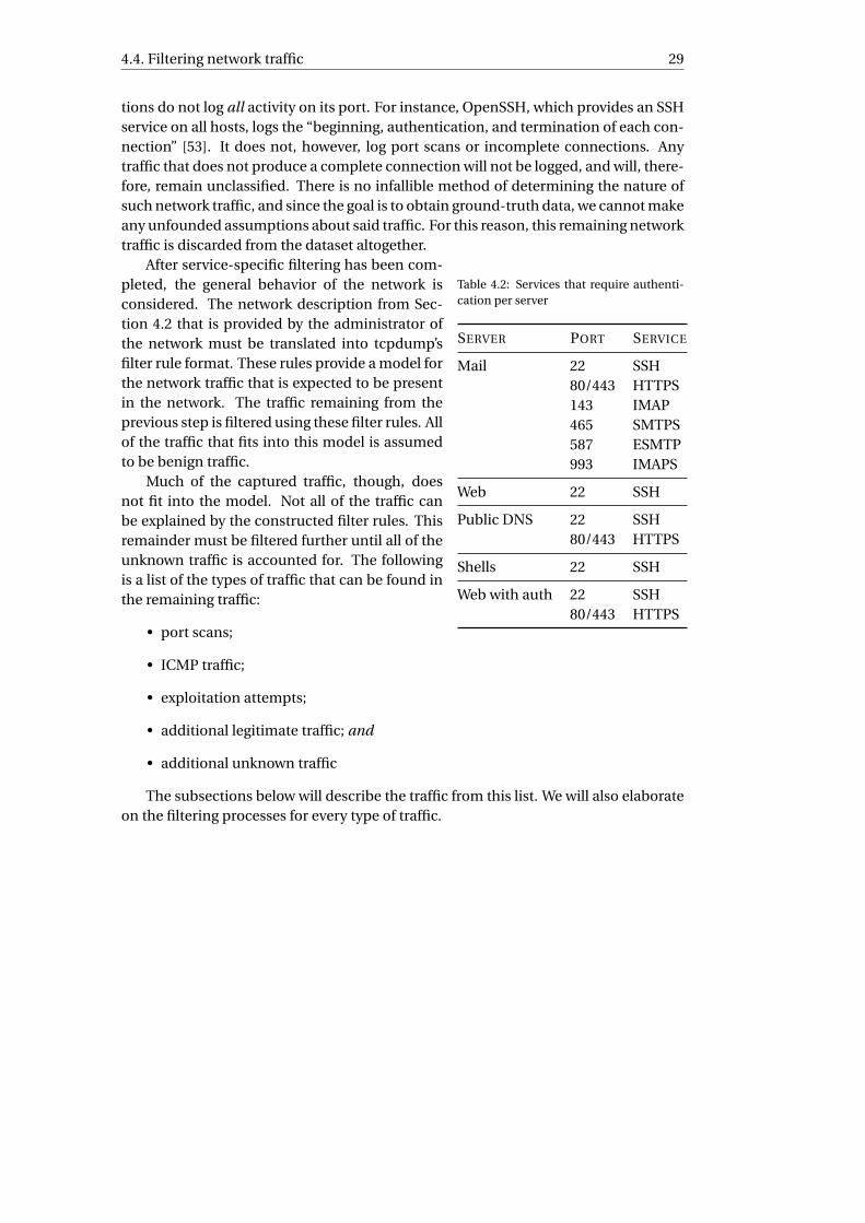
4.4. Filtering network traffic 29
tions do not log all activity on its port. For instance, OpenSSH, which provides an SSHservice on all hosts, logs the “beginning, authentication, and termination of each con-nection” [53]. It does not, however, log port scans or incomplete connections. Anytraffic that does not produce a complete connection will not be logged, and will, there-fore, remain unclassified. There is no infallible method of determining the nature ofsuch network traffic, and since the goal is to obtain ground-truth data, we cannot makeany unfounded assumptions about said traffic. For this reason, this remaining networktraffic is discarded from the dataset altogether.
Table 4.2: Services that require authenti-cation per server
SERVER PORT SERVICE
Mail 22 SSH80/443 HTTPS143 IMAP465 SMTPS587 ESMTP993 IMAPS
Web 22 SSH
Public DNS 22 SSH80/443 HTTPS
Shells 22 SSH
Web with auth 22 SSH80/443 HTTPS
After service-specific filtering has been com-pleted, the general behavior of the network isconsidered. The network description from Sec-tion 4.2 that is provided by the administrator ofthe network must be translated into tcpdump’sfilter rule format. These rules provide a model forthe network traffic that is expected to be presentin the network. The traffic remaining from theprevious step is filtered using these filter rules. Allof the traffic that fits into this model is assumedto be benign traffic.
Much of the captured traffic, though, doesnot fit into the model. Not all of the traffic canbe explained by the constructed filter rules. Thisremainder must be filtered further until all of theunknown traffic is accounted for. The followingis a list of the types of traffic that can be found inthe remaining traffic:
• port scans;
• ICMP traffic;
• exploitation attempts;
• additional legitimate traffic; and
• additional unknown traffic
The subsections below will describe the traffic from this list. We will also elaborateon the filtering processes for every type of traffic.
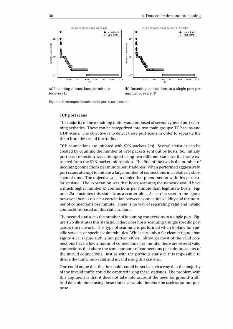
30 4. Data collection and processing
(a) Incoming connections per minutefor every IP
(b) Incoming connections to a single port perminute for every IP
Figure 4.2: Attempted heuristics for port scan detection
TCP port scans
The majority of the remaining traffic was composed of several types of port scan-ning activities. These can be categorized into two main groups: TCP scans andUDP scans. The objective is to detect these port scans in order to separate thethem from the rest of the traffic.
TCP connections are initiated with SYN packets [79]. Several statistics can becreated by counting the number of SYN packets sent out by hosts. So, initially,port scan detection was attempted using two different statistics that were ex-tracted from the SYN packet information. The first of the two is the number ofincoming connections per minute per IP address. When performed aggressively,port scans attempt to initiate a large number of connections in a relatively shortspan of time. The objective was to depict that phenomenon with this particu-lar statistic. The expectation was that hosts scanning the network would havea much higher number of connections per minute than legitimate hosts. Fig-ure 4.2a illustrates this statistic as a scatter plot. As can be seen in the figure,however, there is no clear correlation between connection validity and the num-ber of connections per minute. There is no way of separating valid and invalidconnections based on this statistic alone.
The second statistic is the number of incoming connections to a single port. Fig-ure 4.2b illustrates this statistic. It describes hosts scanning a single specific portacross the network. This type of scanning is performed when looking for spe-cific services or specific vulnerabilities. While certainly a far cleaner figure thanFigure 4.2a, Figure 4.2b is not perfect either. Although most of the valid con-nections have a low amount of connections per minute, there are several validconnections that share the same amount of connections per minute as lots ofthe invalid connections. Just as with the previous statistic, it is impossible todivide the traffic into valid and invalid using this statistic.
One could argue that the thresholds could be set in such a way that the majorityof the invalid traffic could be captured using these statistics. The problem withthis argument is that it does not take into account the need for ground-truth.And data obtained using these statistics would therefore be useless for our pur-pose.
4.4. Filtering network traffic 31
A form of TCP scans is the SYN scan. A side effect of a SYN scan is the creation ofRST packets, either by the host performing the scan, or by the host that is beingscanned [14]. The scanner creates a SYN packet addressed to a specific host andport, and sends it to the target host. In the case that the target port is open, thehost will respond to the scanner with a SYN/ACK packet. The SYN/ACK packettells the scanner that the port is open. After receiving the SYN/ACK packet, thescanner responds with a RST packet to close the connection. If the target portis closed, however, the scanned host does not respond to the scanner with aSYN/ACK packet, but responds with a RST packet instead. In both cases, a RSTpacket is generated by either of the two hosts. Also, since RST packets must begenerated when a port receives packets for which an open connection does notexist [59], we can assume that no legitimate connections will produce RST pack-ets. Hence, the presence of this RST packet can be used to detect SYN scans andthe scanning hosts themselves. The filtering process is then as follows: 1) Forevery RST packet, collect the IP address of the remote host. 2) Extract all of thenetwork traffic corresponding to the collected IP addresses. 3) Classify the ex-tracted traffic as malicious.
Some port scanners, though, do not close the connections they open when scan-ning. Just as the previous case, the scanners send a SYN packet to a certain porton a server, who then responds to the scanner with a SYN/ACK packet. In thestyle of a SYN flood attack [7], the scanner does not to respond to the server witha RST packet, but instead opts to end the connection. This leaves the connec-tion on the server’s side in a half-open state [59]. The server assumes the sentSYN/ACK packet did not successfully arrive at its destination and retransmitsthe packet a number of times before finally closing the connection. Retransmis-sions of the SYN/ACK packets can be identified in the network traffic, and canbe used to detect this type of port scans. The retransmitted SYN/ACK packetsare extracted, and the IP addresses responsible for this traffic are collected. Thetraffic generated by these hosts is then extracted and classified as malicious.
The network traffic captures also contained a number of lone SYN packets origi-nating from remote hosts and addressed to local servers. No matching SYN/ACKpackets appear in the pcap file. Considering there is no firewall or packet fil-ter active on neither the gateway nor the rest of the virtual machines, the SYNpackets could have simply been dropped silently by the virtual machines. Alter-natively, the tcpdump instance could have failed to capture these packets. Eitherway, lone SYN packets that do not attempt to set up a full connection can be in-dicative of port scanning, and, therefore, this traffic should be filtered as well.IP addresses are extracted from the SYN packets, and all traffic corresponding tothose IP addresses is classified as malicious. As mentioned earlier, all TCP con-nections are initiated with SYN packets. By simply filtering out SYN packets, allSYN packets belonging to complete connections will be removed too, be theymalicious or not. It is for this reason that it is important for this step of filteringto be performed last. This ensures that all other traffic has been accounted for,and that lone SYN packets are the only thing left to worry about.
UDP port scans
Seeing as how using connection statistics as in Figure 4.2 did not help with iden-tifying TCP scans, that method was not attempted when trying to identify UDPport scans in the network traffic. Since UDP is a connectionless protocol, there
32 4. Data collection and processing
is no need to use handshakes and establish a connection in order to exchangedata. Given that there is no firewall or filter in place, hosts can just send outany arbitrary UDP datagram to a port listening for UDP traffic, and the port willreceive it [79].
In this network, the only servers that accept UDP traffic are the public DNSserver and the private DNS server. As these two servers are the only users ofUDP traffic, the only legitimate instances of UDP traffic in the network are thefollowing:
– Internal DNS traffic to and from port 53 on the private DNS server.
– Incoming DNS traffic to port 53 on the public DNS server.
– Outgoing DNS traffic from the public DNS server to port 53 on a remoteserver.
Nevertheless, it is wise to avoid using a single blanket filter that captures all butthe aforementioned traffic. Doing so makes it impossible to find possible net-work configuration errors or intrusions that the network administrator is obliv-ious of. Hence, it is interesting to examine the specific instances of UDP scans,because flaws in the network can possibly be identified.
Outside hosts probe many different ports in hope of finding one that respondsto the scan with a UDP packet of their own, thus informing the scanner of anopen port. Many of these attempts are basic scans, but a great deal of them aretargeted scans. Specific ports for which their corresponding services are knownare singled out and receive UDP packets specially crafted for those particularservices. Examples of these include LDAP (Lightweight Directory Access Proto-col) on port 389, SIP (Session Initiation Protocol) on ports 5060 and 5061, andNetBIOS on port 137.
During the examination of the UDP scanning, we discovered an NTP (NetworkTime Protocol) service running on a server where no such service should be run-ning. Upon further investigation by the administrator, it was determined that theNTP service was set up some time in the past for legitimate reasons. The servicewas originally supposed to be running temporarily, but nobody remembered toshut it down afterwards. It could be argued that this traffic should belong withthe rest of the benign traffic, since the service served a legitimate purpose. How-ever, this argument is outweighed by the fact that—by own admission of the net-work administrator—this service is not part of the network’s normal operation.Just because this NTP service turned out to be benign in this particular case,there can be no certainty that no malicious actor will set up an such an NTPservice in the future. Since the classifier should be trained with ground-truthbenign data, placing this traffic with the rest of the benign data will bias the clas-sifier and be of detriment to the results of classification. But because the NTPservice is not malicious either, it cannot be placed with the rest of the malicioustraffic. For this reason, all traffic corresponding to this NTP service was removedcompletely from the dataset.
The rest of the ports receiving UDP packets were examined, and no other irreg-ular incidents were discovered. A filter rule was created for every one of theseports, so that the UDP scans get placed with the malicious traffic.
As none of the other probed services are running on any of the virtual machines,no UDP packets are sent back. Although no server responds to the probes with
4.4. Filtering network traffic 33
UDP packets, closed ports respond to unexpected UDP packets with an ICMPType 3 Code 3 packet (Destination unreachable: Destination port unreachable) [58].ICMP traffic will be discussed in a later section.
Miscellaneous targeted port scans
In the captured traffic, there was one type of port scanning traffic that was nei-ther TCP nor UDP. An outside host was scanning the network for services usingSCTP (Stream Control Transmission Protocol). The network does not run anyservice that uses SCTP, so this is classified as malicious.
ICMP traffic
There are many types of ICMP packets present in the captured traffic. Since thisnetwork operates with both IPv4 and IPv6, both its respective ICMP versionscan be found in the dataset. Different types of these packets serve different pur-poses. Some are part of normal network management traffic, while others can beindicative of malicious activities. Some ICMP traffic can also be used for purelymalicious objectives.
When deciding what ICMP traffic is malicious, we checked out the IP addressesin the packet. The IP addresses were then compared to the lists of valid andinvalid IPs per host and service. If an ICMP packet corresponds to an invalid IPfor a certain service, the packet is placed with the malicious traffic. Conversely,if the packet corresponds to a valid IP and service, the packet is deemed benign.
As mentioned in the UDP port scans section, UDP scans can generate ICMPpackets of the “Destination unreachable” type. The ICMP traffic of this type thatis present in the network traces is the result of UDP scanning. Therefore, thesepackets are part of the malicious traffic and, as such, are classified as malicious.
Ping traffic can be either benign or malicious, depending on the frequency of theping request and the size of the packet. Both the Windows and Linux versions ofthe ping utility sends out one ICMP request per second by default. The networkadministrator has no need for ICMP requests being received by the network ata high frequency. Thus, we set the limit for benign ICMP requests to four persecond for a single host. Any host that sends ICMP requests at this frequency orhigher will have their corresponding ICMP deemed malicious. The rest is placedwith the benign traffic.
An example of a purely malicious instance of ICMP traffic is the Ping of Death [9].This is an IPv4 ICMP packet that is larger than the maximum packet length of anIPv4 packet, which is 65,535 bytes. To extract Ping of Death packets, we createda tcpdump filter rule that examines ICMP packets and their IP header. It thetotal length of the packet exceeds 65,535 bytes, the packet is a malicious one. Allremaining ping traffic is benign.
Furthermore, we also encountered ICMP packets of type Time Exceeded thatoriginate from outside the network. These are ICMP packets that are sent backto a packet’s source by a router when the time-to-live field reaches zero [58]. Thepackets announce that certain DNS packets originating from the public DNSserver did not reach their destination before the expiration of its time-to-livevalue. There is nothing abnormal about either the DNS packet’s destination IPor the contents of the payload. Therefore, a BGP routing loop is the most likelyexplanation as to the cause ICMP Time Exceeded packets. This routing loop
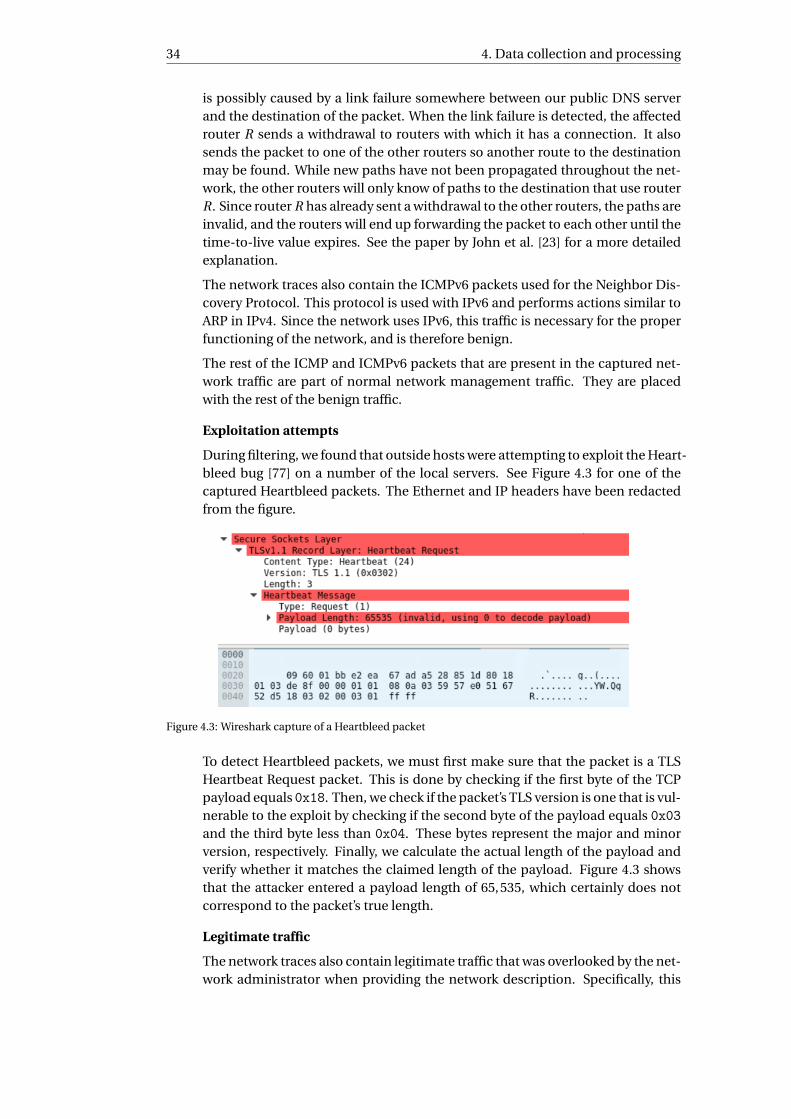
34 4. Data collection and processing
is possibly caused by a link failure somewhere between our public DNS serverand the destination of the packet. When the link failure is detected, the affectedrouter R sends a withdrawal to routers with which it has a connection. It alsosends the packet to one of the other routers so another route to the destinationmay be found. While new paths have not been propagated throughout the net-work, the other routers will only know of paths to the destination that use routerR. Since router R has already sent a withdrawal to the other routers, the paths areinvalid, and the routers will end up forwarding the packet to each other until thetime-to-live value expires. See the paper by John et al. [23] for a more detailedexplanation.
The network traces also contain the ICMPv6 packets used for the Neighbor Dis-covery Protocol. This protocol is used with IPv6 and performs actions similar toARP in IPv4. Since the network uses IPv6, this traffic is necessary for the properfunctioning of the network, and is therefore benign.
The rest of the ICMP and ICMPv6 packets that are present in the captured net-work traffic are part of normal network management traffic. They are placedwith the rest of the benign traffic.
Exploitation attempts
During filtering, we found that outside hosts were attempting to exploit the Heart-bleed bug [77] on a number of the local servers. See Figure 4.3 for one of thecaptured Heartbleed packets. The Ethernet and IP headers have been redactedfrom the figure.
Figure 4.3: Wireshark capture of a Heartbleed packet
To detect Heartbleed packets, we must first make sure that the packet is a TLSHeartbeat Request packet. This is done by checking if the first byte of the TCPpayload equals 0x18. Then, we check if the packet’s TLS version is one that is vul-nerable to the exploit by checking if the second byte of the payload equals 0x03and the third byte less than 0x04. These bytes represent the major and minorversion, respectively. Finally, we calculate the actual length of the payload andverify whether it matches the claimed length of the payload. Figure 4.3 showsthat the attacker entered a payload length of 65,535, which certainly does notcorrespond to the packet’s true length.
Legitimate traffic
The network traces also contain legitimate traffic that was overlooked by the net-work administrator when providing the network description. Specifically, this

4.5. Results of filtering process 35
traffic is composed of network traffic between the Shells server and the IP ad-dress 178.63.40.67 on port 443. This IP address belongs to a chat client website2.Since this is legitimate user traffic, this is placed with the benign traffic.
Unknown traffic
The last portion of unclassified traffic that we encountered was traffic to port443 on the Shells server. This traffic is not supposed to be present, and only oc-curred on a small number of days. Interestingly, none of this traffic is HTTPS,even though it is port 443 that is receiving requests. We know this because theShells server presents an OpenSSH banner when a connection with a host is es-tablished. After examination by the network administrator, no definite explana-tion could be found as to the cause of the OpenSSH service, nor for what purposeit was used. Due to the lack of information on this particular type of networktraffic, we cannot establish the necessary ground-truth. All traffic of this type,namely traffic that corresponds to port 443 on the Shells server, was eliminatedfrom the dataset.
4.5. Results of filtering processFigure 4.4 illustrates the proportion of good, bad, and unclassified traffic before and af-ter the complete filtering process. Specifically, Figure 4.4a illustrates these proportionsafter filtering the traffic using the original description of the network that was providedby the network administrator. Using the filtering rules described in this chapter, wewere able to entirely annotate the unclassified portion of network traffic as good andbad.
An interesting aspect about Figure 4.4a is the increase in unclassified network traf-fic as the days progress. While the original network description was somewhat effectiveat classifying most of the network traffic during the initial portion of the capture, it be-came increasingly difficult to do so later on. This demonstrates the unpredictability oftraffic within a network, and the limited knowledge we have about our own networks.
2https://weechat.org/
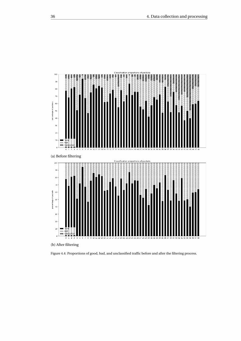
36 4. Data collection and processing
(a) Before filtering
(b) After filtering
Figure 4.4: Proportions of good, bad, and unclassified traffic before and after the filtering process.

5Attack traffic construction
The previous chapter spoke about the network used for the experiment. Its structure,contents, and the different types of traffic that the network receives every day werediscussed. In addition to testing the Kitsune classifier on the everyday traffic of a real-world network, it is interesting to see how well the classifier would fare against networktraffic that is undeniably malicious.
In the research by Mirsky et al. [47], they evaluate the performance of their classifierby simulating a number of attacks on their artificial networks. Nine different attacksare simulated in the network, which can be categorized into four types:
• Reconnaissance: OS scan, fuzzing.
• Man-in-the-Middle: Video injection, ARP poisoning, active wiretap.
• Denial of Service: SSDP flood, SYN flood, SSL renegotiation.
• Botnet Malware: Mirai infection.
After allowing the Kitsune instance to train itself on a stream of benign traffic, oneof these attacks was performed on the network. This process was then repeated forevery attack in the list.
Mirsky et al. have released the datasets of the captured traffic from their networkthat were used in the testing of Kitsune [45] in the form of pcap files. Directly testingour Kitsune instance on this dataset, however, will not provide us with any meaningfulresults. This is because our network, and all the network traffic found within it, differssignificantly from the network used by Mirsky et al. The difference is not only in typeof network traffic (web, mail, SSH, etc. vs. mostly video), but more subtle differences,such as IP and MAC addresses, and network latency. Any of these differences couldgive a classifier enough reason to label certain traffic as malicious, whether or not itactually is.
Therefore, it is necessary to transform the provided datasets to resemble our ownnetwork traffic as closely as possible. Doing so will ensure that our Kitsune instanceis evaluating the attack traffic on the aspects that actually make the traffic malicious,as opposed to, for instance, IP or MAC addresses it as never seen before. On the otherhand, we must not alter the datasets too much. Since the idea is to replicate the evalu-ation performed by Mirsky et al., the altered attack traffic must still resemble the origi-nal attack traffic. Only by ensuring this, will the results obtained from our experiments
37
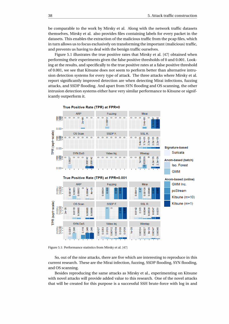
38 5. Attack traffic construction
be comparable to the work by Mirsky et al. Along with the network traffic datasetsthemselves, Mirsky et al. also provides files containing labels for every packet in thedatasets. This enables the extraction of the malicious traffic from the pcap files, whichin turn allows us to focus exclusively on transforming the important (malicious) traffic,and prevents us having to deal with the benign traffic ourselves.
Figure 5.1 illustrates the true positive rates that Mirsky et al. [47] obtained whenperforming their experiments given the false positive thresholds of 0 and 0.001. Look-ing at the results, and specifically to the true positive rates at a false positive thresholdof 0.001, we see that Kitsune does not seem to perform better than alternative intru-sion detection systems for every type of attack. The three attacks where Mirsky et al.report significantly improved detection are when detecting Mirai infections, fuzzingattacks, and SSDP flooding. And apart from SYN flooding and OS scanning, the otherintrusion detection systems either have very similar performance to Kitsune or signif-icantly outperform it.
Figure 5.1: Performance statistics from Mirsky et al. [47]
So, out of the nine attacks, there are five which are interesting to reproduce in thiscurrent research. These are the Mirai infection, fuzzing, SSDP flooding, SYN flooding,and OS scanning.
Besides reproducing the same attacks as Mirsky et al., experimenting on Kitsunewith novel attacks will provide added value to this research. One of the novel attacksthat will be created for this purpose is a successful SSH brute-force with log in and
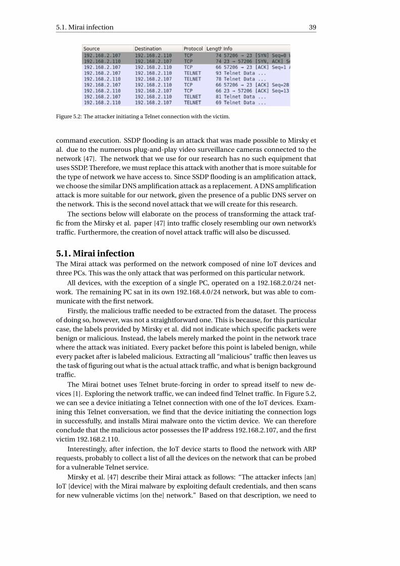
5.1. Mirai infection 39
Figure 5.2: The attacker initiating a Telnet connection with the victim.
command execution. SSDP flooding is an attack that was made possible to Mirsky etal. due to the numerous plug-and-play video surveillance cameras connected to thenetwork [47]. The network that we use for our research has no such equipment thatuses SSDP. Therefore, we must replace this attack with another that is more suitable forthe type of network we have access to. Since SSDP flooding is an amplification attack,we choose the similar DNS amplification attack as a replacement. A DNS amplificationattack is more suitable for our network, given the presence of a public DNS server onthe network. This is the second novel attack that we will create for this research.
The sections below will elaborate on the process of transforming the attack traf-fic from the Mirsky et al. paper [47] into traffic closely resembling our own network’straffic. Furthermore, the creation of novel attack traffic will also be discussed.
5.1. Mirai infectionThe Mirai attack was performed on the network composed of nine IoT devices andthree PCs. This was the only attack that was performed on this particular network.
All devices, with the exception of a single PC, operated on a 192.168.2.0/24 net-work. The remaining PC sat in its own 192.168.4.0/24 network, but was able to com-municate with the first network.
Firstly, the malicious traffic needed to be extracted from the dataset. The processof doing so, however, was not a straightforward one. This is because, for this particularcase, the labels provided by Mirsky et al. did not indicate which specific packets werebenign or malicious. Instead, the labels merely marked the point in the network tracewhere the attack was initiated. Every packet before this point is labeled benign, whileevery packet after is labeled malicious. Extracting all “malicious” traffic then leaves usthe task of figuring out what is the actual attack traffic, and what is benign backgroundtraffic.
The Mirai botnet uses Telnet brute-forcing in order to spread itself to new de-vices [1]. Exploring the network traffic, we can indeed find Telnet traffic. In Figure 5.2,we can see a device initiating a Telnet connection with one of the IoT devices. Exam-ining this Telnet conversation, we find that the device initiating the connection logsin successfully, and installs Mirai malware onto the victim device. We can thereforeconclude that the malicious actor possesses the IP address 192.168.2.107, and the firstvictim 192.168.2.110.
Interestingly, after infection, the IoT device starts to flood the network with ARPrequests, probably to collect a list of all the devices on the network that can be probedfor a vulnerable Telnet service.
Mirsky et al. [47] describe their Mirai attack as follows: “The attacker infects [an]IoT [device] with the Mirai malware by exploiting default credentials, and then scansfor new vulnerable victims [on the] network.” Based on that description, we need to
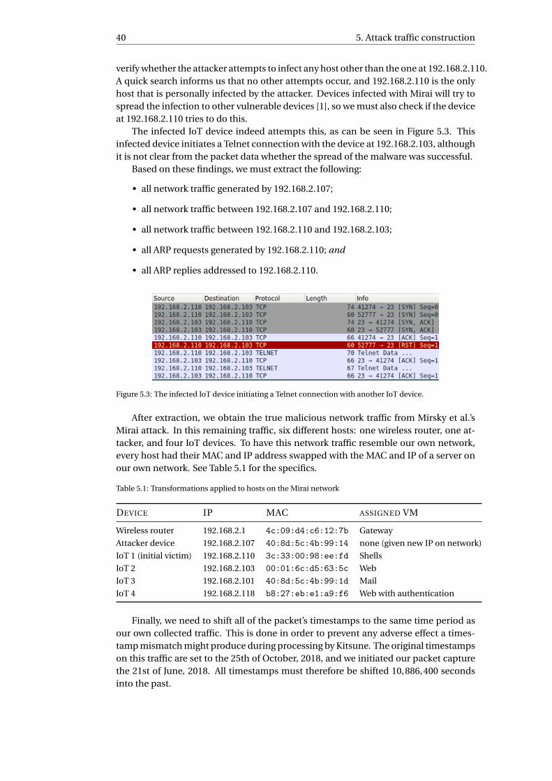
40 5. Attack traffic construction
verify whether the attacker attempts to infect any host other than the one at 192.168.2.110.A quick search informs us that no other attempts occur, and 192.168.2.110 is the onlyhost that is personally infected by the attacker. Devices infected with Mirai will try tospread the infection to other vulnerable devices [1], so we must also check if the deviceat 192.168.2.110 tries to do this.
The infected IoT device indeed attempts this, as can be seen in Figure 5.3. Thisinfected device initiates a Telnet connection with the device at 192.168.2.103, althoughit is not clear from the packet data whether the spread of the malware was successful.
Based on these findings, we must extract the following:
• all network traffic generated by 192.168.2.107;
• all network traffic between 192.168.2.107 and 192.168.2.110;
• all network traffic between 192.168.2.110 and 192.168.2.103;
• all ARP requests generated by 192.168.2.110; and
• all ARP replies addressed to 192.168.2.110.
Figure 5.3: The infected IoT device initiating a Telnet connection with another IoT device.
After extraction, we obtain the true malicious network traffic from Mirsky et al.’sMirai attack. In this remaining traffic, six different hosts: one wireless router, one at-tacker, and four IoT devices. To have this network traffic resemble our own network,every host had their MAC and IP address swapped with the MAC and IP of a server onour own network. See Table 5.1 for the specifics.
Table 5.1: Transformations applied to hosts on the Mirai network
DEVICE IP MAC ASSIGNED VM
Wireless router 192.168.2.1 4c:09:d4:c6:12:7b Gateway
Attacker device 192.168.2.107 40:8d:5c:4b:99:14 none (given new IP on network)
IoT 1 (initial victim) 192.168.2.110 3c:33:00:98:ee:fd Shells
IoT 2 192.168.2.103 00:01:6c:d5:63:5c Web
IoT 3 192.168.2.101 40:8d:5c:4b:99:1d Mail
IoT 4 192.168.2.118 b8:27:eb:e1:a9:f6 Web with authentication
Finally, we need to shift all of the packet’s timestamps to the same time period asour own collected traffic. This is done in order to prevent any adverse effect a times-tamp mismatch might produce during processing by Kitsune. The original timestampson this traffic are set to the 25th of October, 2018, and we initiated our packet capturethe 21st of June, 2018. All timestamps must therefore be shifted 10,886,400 secondsinto the past.
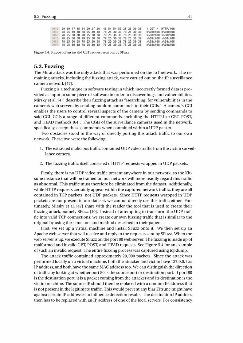
5.2. Fuzzing 41
Figure 5.4: Snippet of an invalid GET request sent out by SFuzz
5.2. FuzzingThe Mirai attack was the only attack that was performed on the IoT network. The re-maining attacks, including the fuzzing attack, were carried out on the IP surveillancecamera network [47].
Fuzzing is a technique in software testing in which incorrectly formed data is pro-vided as input to some piece of software in order to discover bugs and vulnerabilities.Mirsky et al. [47] describe their fuzzing attack as “[searching] for vulnerabilities in thecamera’s web servers by sending random commands to their CGIs.” A camera’s CGIenables the users to control several aspects of the camera by sending commands tosaid CGI. CGIs a range of different commands, including the HTTP-like GET, POST,and HEAD methods [64]. The CGIs of the surveillance cameras used in the network,specifically, accept these commands when contained within a UDP packet.
Two obstacles stood in the way of directly porting this attack traffic to our ownnetwork. These two were the following:
1. The extracted malicious traffic contained UDP video traffic from the victim surveil-lance camera.
2. The fuzzing traffic itself consisted of HTTP requests wrapped in UDP packets.
Firstly, there is no UDP video traffic present anywhere in our network, so the Kit-sune instance that will be trained on our network will more readily regard this trafficas abnormal. This traffic must therefore be eliminated from the dataset. Additionally,while HTTP requests certainly appear within the captured network traffic, they are allcontained in TCP packets, not UDP packets. Since HTTP requests wrapped in UDPpackets are not present in our dataset, we cannot directly use this traffic either. For-tunately, Mirsky et al. [47] share with the reader the tool that is used to create theirfuzzing attack, namely SFuzz [10]. Instead of attempting to transform the UDP traf-fic into valid TCP connections, we create our own fuzzing traffic that is similar to theoriginal by using the same tool and method described in their paper.
First, we set up a virtual machine and install SFuzz onto it. We then set up anApache web server that will receive and reply to the requests sent by SFuzz. When theweb server is up, we execute SFuzz on the port 80 web server. The fuzzing is made up ofmalformed and invalid GET, POST, and HEAD requests. See Figure 5.4 for an exampleof such an invalid request. The entire fuzzing process was captured using tcpdump.
The attack traffic contained approximately 20,000 packets. Since the attack wasperformed locally on a virtual machine, both the attacker and victim have 127.0.0.1 asIP address, and both have the same MAC address too. We can distinguish the directionof traffic by looking at whether port 80 is the source port or destination port. If port 80is the destination port, it is a packet coming from the attacker and its destination is thevictim machine. The source IP should then be replaced with a random IP address thatis not present in the legitimate traffic. This would prevent any bias Kitsune might haveagainst certain IP addresses to influence detection results. The destination IP addressthen has to be replaced with an IP address of one of the local servers. For consistency
42 5. Attack traffic construction
with our network, we replace this destination IP address with the IP address of theWeb server. If port 80 is the source port, then the packet is a reply to the attackercoming from the web server. The source IP is then replaced with the IP address of ourWeb server, and the destination IP is replaced with the randomly chosen IP address.Furthermore, MAC addresses need to be fixed according to the working of our network:in case of incoming traffic (i.e. fuzzing traffic addressed to our Web server), the sourceMAC is replaced with a previously-unseen MAC, and the destination MAC is replacedwith the MAC of our network’s Gateway VM. Outgoing packets get the source MAC ofour Web server, and the randomly chosen MAC address as destination MAC.
5.3. SYN flooding
A SYN flood is a denial-of-service attack in which an attacker sends out of SYN requeststo a certain server. The objective is to consume all of the victim’s server resources inorder to prevent the server from providing its service to legitimate users.
The SYN flooding attack dataset is also one that is released by Mirsky et al. [45]The attack is performed using the hping3 tool [67]. The attacker sends a flood of SYNpackets to the web server (HTTP port 80) of a single video surveillance camera, whichcauses its video stream to halt. The source IP address in the SYN packets are spoofedand replaced with random IP addresses. This dataset contains normal video trafficover UDP and over HTTPS. The malicious traffic itself that is present in the datasetconsists of the SYN/ACK packets that the victim camera sends out in response to theincoming SYN requests, as well as retransmissions of these SYN/ACK packets whenno ACK packet is received from the spoofed IP addresses. The original malicious SYNpackets are not available in the dataset, because these packets did not reach the seg-ment of the network where Mirsky et al. had set up their Kitsune instance [47].
This situation would not occur in our case, since all of the servers are connectedto a central gateway. Therefore, this dataset is not suitable for our experiments, andwe must create our own SYN flood dataset that is more appropriate for our type ofnetwork.
For our dataset, we decided to simulate a 100 Mbps SYN flood. A single SYN packetis 60 bytes, meaning that a 100 Mbps SYN flood would have to contain around 210,000SYN packets per second. Just like the dataset released by Mirsky et al., these SYN pack-ets contain spoofed source IP addresses. In the original dataset, the SYN packets wereaddressed to a web server on port 80. For the newly created dataset, the SYN packetsare addressed to port 80 of our own Web server. Finally, it is necessary to ensure thatthe SYN packet’s timestamps correspond to the 21st of June, 2018. This dataset wasconstructed with the use of Scapy.
However, this dataset that was created has two limitations that were not possibleto avoid due to them being caused by Kitsune itself. The Python version of Kitsunethat is released by Mirsky et al. [44] can consume a great deal of memory when deal-ing with large surges of traffic. Much more than the unreleased C++ version of theIDS [47]. Because of these issues with memory consumption, we were forced to limitthe number of SYN packets to a just million packets. In a 100 Mbps SYN flood, this isapproximately five seconds worth of traffic. Also, every new IP address creates a newincremental statistic tuple, consuming more memory in the process. As a result, wealso limited the randomization of the source IP addresses. All spoofed addresses are ofthe form 123.123.123.x, where x is the only randomized portion of the IP address.
5.4. OS scanning 43
5.4. OS scanningThe OS scan dataset is also one that is released by Mirsky et al. [45] This attack is de-scribed as “[an] attacker [scanning] the network for hosts, and their operating systems,to reveal possible vulnerabilities.” [47] In reality, the OS scan differs from what is de-scribed by Mirsky et al. in their paper. What actually occurs in the scan traffic is thatthe attacker targets a single host and scans this host by sending a single SYN request toevery port (1-65535). No separate scan was conducted for UDP service discovery.
The IP address of the host performing the OS scan is 192.168.2.7. This address isused only by the attacker, and only for the purpose of scanning the target host. The IPaddress of the host being scanned is 192.168.2.1, meaning that the attacker and the vic-tim are on the same subnet (assuming a /24 network). Seeing as this is the way Mirskyet al. performed their experiment, we must make sure that our version differs as littleas possible. To this end, we replace the IP address of the attacker with a completelynew IP address that would place the attacker inside our network (again, assuming a/24 network). We replace the victim’s IP address with the IP address of the Web server.The MAC addresses are also altered: the attacker’s MAC is changed to the MAC addressof the Gateway VM, and the victim’s MAC address is changed to that of the Web server.
5.5. Successful SSH brute-forceThe successful SSH brute-force attack is another novel attack that we created for thepurpose of our research. We wanted to test Kitsune’s detection abilities in a scenariowhere an attacker uses readily available tools to successfully brute-force the passwordbelonging to the admin user on an open SSH service, logs in using the found password,and executes some commands on the remote host. We set up a virtual machine wecould perform the attack on, and all traffic was captured using tcpdump.
In order to perform a brute-force attack, an attacker sometimes uses a list con-taining a collection of commonly-used passwords. We constructed such a list, whichcontains 1141 passwords. Of the 1141, only the last password in the list is the correctone. An SSH server was set up on a virtual machine, and the hydra tool [82] was used tolaunch the brute-force attack. As the attacker, we launched hydra with 16 parallel tasksto speed up the brute-force attack. Since the correct password is the last element in thelist of 1141, the brute-force attack had 1140 failed attempts before finally succeedingat attempt number 1141. After the successful brute-force and finding the correct pass-word, the attacker then logs in to the remote SSH service using the acquired passwordand executes the commands “cat /etc/passwd” and “cat /etc/shadow” before ex-iting.
Because the attack was not performed on the actual network, but instead in a vir-tual machine, the pcap file must be altered before it can be used. First of all, the IPaddress of the attacker should be an IP address that is not present in the legitimatetraffic. Again, this is to prevent any bias Kitsune might have against IP addresses it hasalready seen. Secondly, the victim’s IP address should be replaced with the IP addressof one of the local servers. It is important to keep the attack traffic consistent with thefunctionality offered by the servers on the network. Although all servers offer an SSHservice, the Shells server is the only one that has this service as its primary function.The Shells server would send and receive much more SSH traffic than the rest of theservers. It is possible that Kitsune would see a spike in SSH traffic to the other serversas malicious—regardless of whether it actually is—simply because it is a spike that itis not used to seeing. To prevent this other bias from influencing the results, we choseto assign the IP address of the Shells server to the victim of the brute-force. Lastly, the
44 5. Attack traffic construction
MAC address of the victim should also be replaced with the MAC address of the Shellsserver.
5.6. DNS abuse and DNS amplificationThis section describes three different attacks that we created. All three are related toeach other. The first two contains traffic that abuses the functionality of the publicDNS server. The last attack is an incoming DNS amplification attack that resulted fromthe abuse of external open DNS servers.
DNS amplification attack. In a DNS amplification attack, an attacker sends DNSqueries with a spoofed source IP to open DNS servers, which causes the DNS serversto flood the victim with all the DNS responses [8]. Since the size of DNS responses islarger than the query sent by the attacker, the amount of traffic that reaches the victimis amplified by the DNS servers. DNS amplification attacks are a very common typeof attack, making up 18.6% of all DDoS attacks on the Internet [22]. The network usedfor this research contains such an open DNS server that could potentially be used tocarry out DNS amplification attacks. Therefore, it is interesting to see whether Kitsuneis able to detect such a scenario, and also whether it is able to detect such an incomingattack itself.
When abusing open DNS servers for DNS amplification attacks, attackers will of-tentimes use ANY queries for DNS amplification attacks, as this results in the largestpossible DNS response [8]. The public DNS server on our network, however, does notaccept DNS queries of type ANY over UDP. It only accepts ANY queries over TCP. Analternative that also amplifies traffic significantly is the request of an MX record. Forexample, one incoming 88 byte MX query to the public DNS server produced a 492byte response. The public DNS server has no restrictions on querying MX records overUDP.
We extracted the aforementioned MX query and response from the DNS traffic.This two packets form be the basis of the DNS amplification attack. Using Scapy, wereplaced the source IP of the query and the destination IP of the response with a ran-domized IP address that is not present in the legitimate traffic. This IP address willrepresent the victim’s IP address. In order to avoid the same memory issues as in theSYN flood case, we reduced the total number of packets to 200,000. Half of these pack-ets are DNS queries, while the other half are DNS responses.
To examine the effect of the frequency with which the DNS queries are sent, wecreated to variations of this attack. The first version has the queries sent with a fre-quency of 100 DNS queries per millisecond, while the second version does it at a lowerfrequency of one DNS query per millisecond.
The DNS amplification attack itself was also constructed using the extracted DNStransaction. The difference with the previous two scenarios is that only the DNS re-sponse was used to create the attack. Since a DNS amplification attack is a floodof DNS responses, this is the only packet that is necessary. We simulated an attackwhere 10 external servers would flood the Web server with DNS response traffic. Tothis end, the source IP of the packet was replaced with one of 10 randomly chosen andpreviously-unseen IP addresses. The source MAC address was replaced with the MACaddress of the Gateway VM. Because the Web server is the host that is being attacked,the destination IP and MAC addresses were replaced with those corresponding to theWeb server. The DNS responses are received at a packet rate of 100 packets per mil-lisecond.
6IDS evaluation
Previous chapters described the preparation of the datasets that we used for the ex-periments. This chapter will begin by elaborating on the methodology we followed toperform the evaluation of the Kitsune IDS. Afterwards, we present the results obtainedfrom the evaluation process. These results include Kitsune’s performance on everydaydata, as well as on actual attack traffic.
6.1. Performance evaluationOnce we have downloaded the Kitsune IDS [44] and installed it onto our machines, wemust train it in the manner Mirsky et al. [47] did. Proper performance evaluation isonly possible when sufficient data is captured, and all of this data is properly filteredand separated into legitimate and illegitimate traffic.
Mirsky et al. make the objective of their research to create an IDS that uses unsu-pervised learning [47]. They state this as an objective due to the difficulty encounteredby supervised learning IDSs when trying to detect previously-unseen malicious traffic.Afterwards, they also state that Kitsune must be trained on “normal data” [47]. There-fore, we must test Kitsune in two different manners.
In the first, we will train Kitsune on all of the ground-truth legitimate data obtainedfrom the first day of capturing. Because we are training on all of the legitimate data in-stead of just a portion, this will function as a best-case scenario for Kitsune’s detectionperformance. After training on the legitimate data, we will merge the legitimate andillegitimate traffic into a single dataset and attempt to detect the illegitimate trafficwith Kitsune. An additional experiment will be performed. We will inject attack trafficinto our network traces. Then, the trained Kitsune instance will be tasked with pro-cessing the altered network trace and detect this malicious attack traffic. Specifically,we will use the benign portion of the first day of captured traffic for this experiment.We choose this portion of the network trace, since it is the same data with which wewill train our Kitsune instance. To maintain consistency with their work, we will useattack traffic that is as similar as possible to the attack traffic used by by Mirsky etal. [47]. Mirsky et al. have released their attack traffic to the public [45]. We will usethese datasets for own experiments. This research will also contain attacks that havenot been performed by Mirsky et al. [47] A detailed explanation as to the generationof this attack traffic can be found in Chapter 5. In Chapter 3, we describe Kitsune’s mparameter. Mirsky et al. perform their experiments in two different scenarios: (i) us-ing a maximum autoencoder size m = 10, and (ii) using a maximum autoencoder size
45
46 6. IDS evaluation
m = 1 [47]. To maintain consistency between this research and that by Mirsky et al., wewill also perform these experiments using both parameters.
The reason for Kitsune making use of unsupervised learning is so that it can beable to detect previously-unseen attacks as malicious traffic [47]. We must thereforeperform a second type of test on Kitsune’s detection performance. Instead of train-ing Kitsune on only the legitimate traffic, we now train Kitsune on the full first day ofcaptured network traffic. After training, we have Kitsune process the network tracesfrom the rest of the captured days. The goal of this second test is to determine whetherKitsune is able to detect previously-unseen traffic if trained on realistic, noisy data.
Section 2.3 discussed many types of techniques and measures that are used for theperformance evaluation of anomaly detection systems. Of all the performance met-rics, Mirsky et al. focus on the following four: false positive rate, true positive rate,AUC, and equal error rate. Again, for the sake of consistency and to provide a truecomparison of performance, we will also focus on these metrics during evaluation inthis project.
6.2. Classifying everyday network trafficWe collected seven weeks of network traffic. Two experiments were performed usingjust this captured data to test both Kitsune’s detection performance and claims madeby Mirsky et al. [47] about their IDS. In the first experiment, we trained Kitsune on theground-truth benign data filtered from the first day of capturing, and then processedthe benign and malicious traffic from the remaining days. The second experiment hadKitsune trained on both the benign and malicious parts of the first day of capturedtraffic. Kitsune then processed the remaining traffic in an attempt to detect previously-unseen attack traffic. This section will discuss the results obtained from these twoexperiments.
6.2.1. Detecting anomaliesAfter obtaining ground-truth benign and malicious traffic for all of the seven weeksof traffic, we trained Kitsune on the benign data of the first day of capturing. Wefirst trained Kitsune using the parameter m = 10. The detection thresholds were de-termined by having our trained Kitsune instance process the same benign data withwhich it was trained. For F PR = 0.001 and F PR = 0, this yielded as thresholds ap-proximately 0.1857 and 7.460, respectively. We then used the trained Kitsune instanceto process the remaining 48 days of traffic and we recorded the anomaly scored pro-duced by Kitsune. This process was repeated using the parameter m = 1. In this case,the detection thresholds for F PR = 0.001 and F PR = 0 were approximately 0.2021 and6.2696, respectively. The false positive rates and false negative rates were computedusing the detection thresholds. See Figures 6.1 and 6.2 for the false positive rates andfalse negative rates for all seven weeks of captured traffic for m = 10 and m = 1, respec-tively.
Table 6.1: Average FPRs and FNRs, using the thresholds obtained from the first day of network traffic
m = 10 m = 1F PR = 0.001 F PR = 0 F PR = 0.001 F PR = 0
actual FPR 0.064313 0.000002 0.057190 0.000002actual FNR 0.999870 0.999998 0.999039 0.999998
6.2. Classifying everyday network traffic 47
As can be seen from both Figures 6.1a and 6.2a, Kitsune’s FPRs are minuscule whenusing the F PR = 0 threshold. When looking at Figures 6.1b and 6.2b, however, we seethat this low FPR comes at a price, namely an extremely high FNR. For every day, Kit-sune does not produce an FNR lower than 0.97. This is the case for both thresholds,and for both m = 10 and m = 1. Therefore, while Kitsune rarely classifies normal trafficas malicious, detection of actual malicious traffic occurs much less frequently. Ta-ble 6.1 contains the average FPRs and FNRs from Kitsune’s anomaly detection.
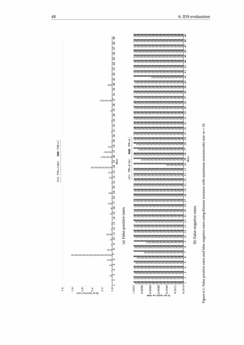
48 6. IDS evaluation
(a)
Fals
ep
osi
tive
rate
s
(b)
Fals
en
egat
ive
rate
s
Fig
ure
6.1:
Fals
ep
osi
tive
rate
san
dfa
lse
neg
ativ
era
tes
usi
ng
Kit
sun
ein
stan
cew
ith
max
imu
mau
toen
cod
ersi
zem
=10
.
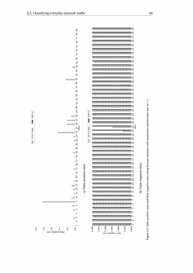
6.2. Classifying everyday network traffic 49
(a)
Fals
ep
osi
tive
rate
s
(b)
Fals
en
egat
ive
rate
s
Fig
ure
6.2:
Fals
ep
osi
tive
rate
san
dfa
lse
neg
ativ
era
tes
usi
ng
Kit
sun
ein
stan
cew
ith
max
imu
mau
toen
cod
ersi
zem
=1.
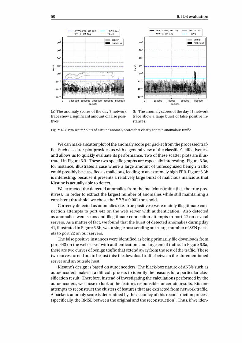
50 6. IDS evaluation
(a) The anomaly scores of the day 7 networktrace show a significant amount of false posi-tives.
(b) The anomaly scores of the day 41 networktrace show a large burst of false positive in-stances.
Figure 6.3: Two scatter plots of Kitsune anomaly scores that clearly contain anomalous traffic
We can make a scatter plot of the anomaly score per packet from the processed traf-fic. Such a scatter plot provides us with a general view of the classifier’s effectivenessand allows us to quickly evaluate its performance. Two of these scatter plots are illus-trated in Figure 6.3. These two specific graphs are especially interesting. Figure 6.3a,for instance, illustrates a case where a large amount of unrecognized benign trafficcould possibly be classified as malicious, leading to an extremely high FPR. Figure 6.3bis interesting, because it presents a relatively large burst of malicious malicious thatKitsune is actually able to detect.
We extracted the detected anomalies from the malicious traffic (i.e. the true pos-itives). In order to extract the largest number of anomalies while still maintaining aconsistent threshold, we chose the F PR = 0.001 threshold.
Correctly detected as anomalies (i.e. true positives) were mainly illegitimate con-nection attempts to port 443 on the web server with authentication. Also detectedas anomalies were scans and illegitimate connection attempts to port 22 on severalservers. As a matter of fact, we found that the burst of detected anomalies during day41, illustrated in Figure 6.3b, was a single host sending out a large number of SYN pack-ets to port 22 on our servers.
The false positive instances were identified as being primarily file downloads fromport 443 on the web server with authentication, and large email traffic. In Figure 6.3a,there are two curves of benign traffic that extend away from the rest of the traffic. Thesetwo curves turned out to be just this: file download traffic between the aforementionedserver and an outside host.
Kitsune’s design is based on autoencoders. The black-box nature of ANNs such asautoencoders makes it a difficult process to identify the reasons for a particular clas-sification result. Therefore, instead of investigating the calculations performed by theautoencoders, we chose to look at the features responsible for certain results. Kitsuneattempts to reconstruct the clusters of features that are extracted from network traffic.A packet’s anomaly score is determined by the accuracy of this reconstruction process(specifically, the RMSE between the original and the reconstruction). Thus, if we iden-
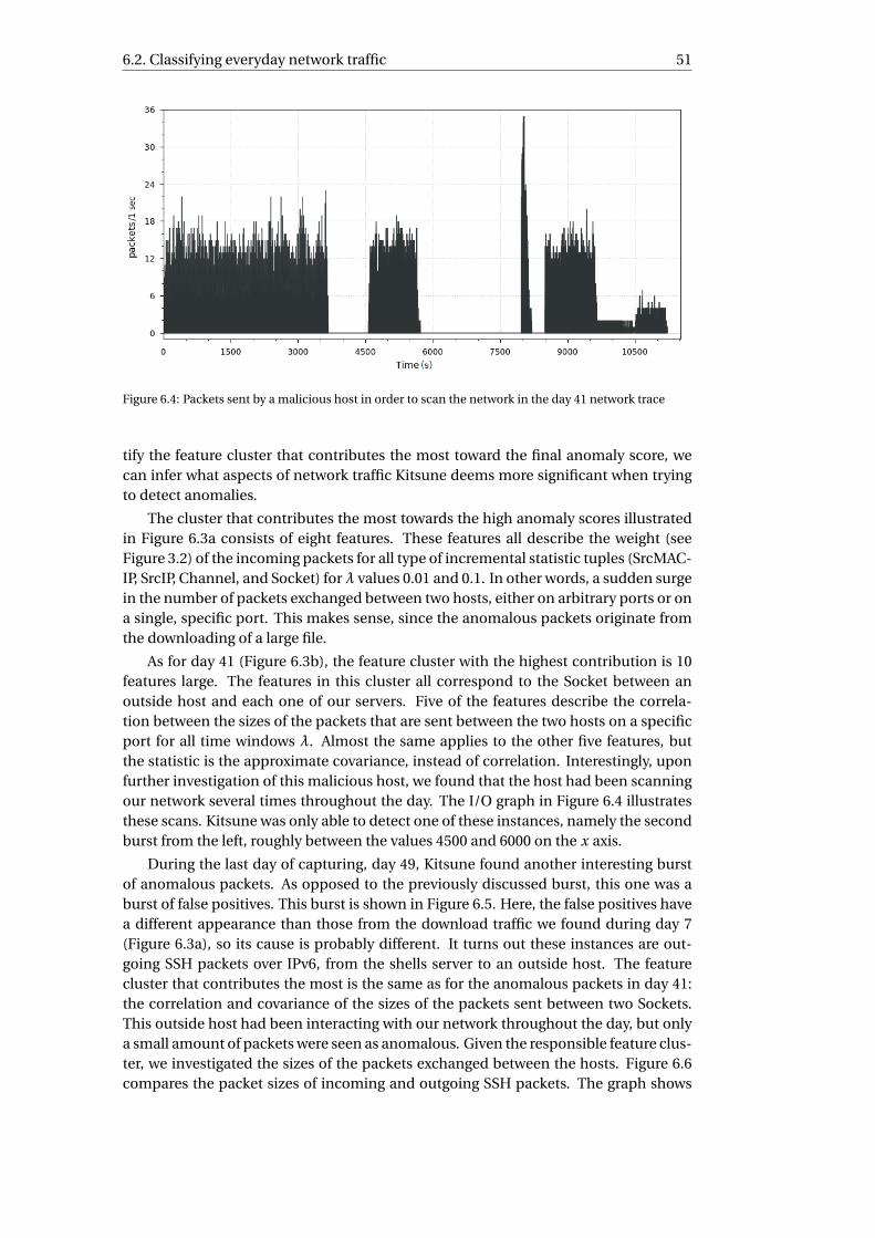
6.2. Classifying everyday network traffic 51
Figure 6.4: Packets sent by a malicious host in order to scan the network in the day 41 network trace
tify the feature cluster that contributes the most toward the final anomaly score, wecan infer what aspects of network traffic Kitsune deems more significant when tryingto detect anomalies.
The cluster that contributes the most towards the high anomaly scores illustratedin Figure 6.3a consists of eight features. These features all describe the weight (seeFigure 3.2) of the incoming packets for all type of incremental statistic tuples (SrcMAC-IP, SrcIP, Channel, and Socket) for λ values 0.01 and 0.1. In other words, a sudden surgein the number of packets exchanged between two hosts, either on arbitrary ports or ona single, specific port. This makes sense, since the anomalous packets originate fromthe downloading of a large file.
As for day 41 (Figure 6.3b), the feature cluster with the highest contribution is 10features large. The features in this cluster all correspond to the Socket between anoutside host and each one of our servers. Five of the features describe the correla-tion between the sizes of the packets that are sent between the two hosts on a specificport for all time windows λ. Almost the same applies to the other five features, butthe statistic is the approximate covariance, instead of correlation. Interestingly, uponfurther investigation of this malicious host, we found that the host had been scanningour network several times throughout the day. The I/O graph in Figure 6.4 illustratesthese scans. Kitsune was only able to detect one of these instances, namely the secondburst from the left, roughly between the values 4500 and 6000 on the x axis.
During the last day of capturing, day 49, Kitsune found another interesting burstof anomalous packets. As opposed to the previously discussed burst, this one was aburst of false positives. This burst is shown in Figure 6.5. Here, the false positives havea different appearance than those from the download traffic we found during day 7(Figure 6.3a), so its cause is probably different. It turns out these instances are out-going SSH packets over IPv6, from the shells server to an outside host. The featurecluster that contributes the most is the same as for the anomalous packets in day 41:the correlation and covariance of the sizes of the packets sent between two Sockets.This outside host had been interacting with our network throughout the day, but onlya small amount of packets were seen as anomalous. Given the responsible feature clus-ter, we investigated the sizes of the packets exchanged between the hosts. Figure 6.6compares the packet sizes of incoming and outgoing SSH packets. The graph shows
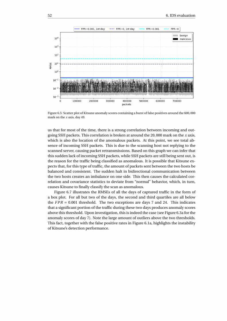
52 6. IDS evaluation
Figure 6.5: Scatter plot of Kitsune anomaly scores containing a burst of false positives around the 600,000mark on the x axis, day 49.
us that for most of the time, there is a strong correlation between incoming and out-going SSH packets. This correlation is broken at around the 20,000 mark on the x axis,which is also the location of the anomalous packets. At this point, we see total ab-sence of incoming SSH packets. This is due to the scanning host not replying to thescanned server, causing packet retransmissions. Based on this graph we can infer thatthis sudden lack of incoming SSH packets, while SSH packets are still being sent out, isthe reason for the traffic being classified as anomalous. It is possible that Kitsune ex-pects that, for this type of traffic, the amount of packets sent between the two hosts bebalanced and consistent. The sudden halt in bidirectional communication betweenthe two hosts creates an imbalance on one side. This then causes the calculated cor-relation and covariance statistics to deviate from “normal” behavior, which, in turn,causes Kitsune to finally classify the scan as anomalous.
Figure 6.7 illustrates the RMSEs of all the days of captured traffic in the form ofa box plot. For all but two of the days, the second and third quartiles are all belowthe F PR = 0.001 threshold. The two exceptions are days 7 and 24. This indicatesthat a significant portion of the traffic during these two days produces anomaly scoresabove this threshold. Upon investigation, this is indeed the case (see Figure 6.3a for theanomaly scores of day 7). Note the large amount of outliers above the two thresholds.This fact, together with the false positive rates in Figure 6.1a, highlights the instabilityof Kitsune’s detection performance.
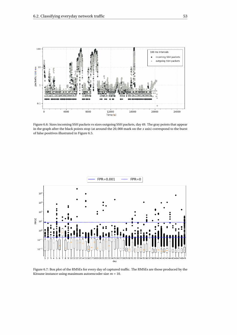
6.2. Classifying everyday network traffic 53
Figure 6.6: Sizes incoming SSH packets vs sizes outgoing SSH packets, day 49. The gray points that appearin the graph after the black points stop (at around the 20,000 mark on the x axis) correspond to the burstof false positives illustrated in Figure 6.5.
Figure 6.7: Box plot of the RMSEs for every day of captured traffic. The RMSEs are those produced by theKitsune instance using maximum autoencoder size m = 10.
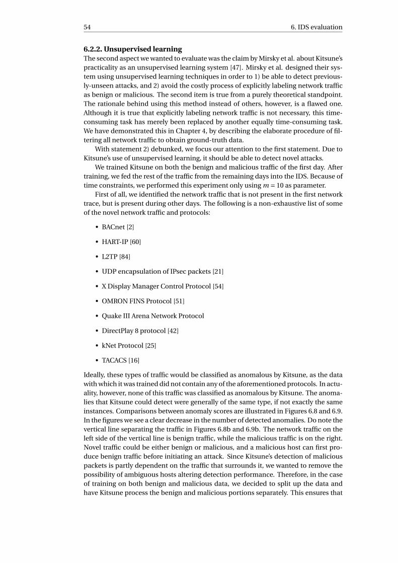
54 6. IDS evaluation
6.2.2. Unsupervised learningThe second aspect we wanted to evaluate was the claim by Mirsky et al. about Kitsune’spracticality as an unsupervised learning system [47]. Mirsky et al. designed their sys-tem using unsupervised learning techniques in order to 1) be able to detect previous-ly-unseen attacks, and 2) avoid the costly process of explicitly labeling network trafficas benign or malicious. The second item is true from a purely theoretical standpoint.The rationale behind using this method instead of others, however, is a flawed one.Although it is true that explicitly labeling network traffic is not necessary, this time-consuming task has merely been replaced by another equally time-consuming task.We have demonstrated this in Chapter 4, by describing the elaborate procedure of fil-tering all network traffic to obtain ground-truth data.
With statement 2) debunked, we focus our attention to the first statement. Due toKitsune’s use of unsupervised learning, it should be able to detect novel attacks.
We trained Kitsune on both the benign and malicious traffic of the first day. Aftertraining, we fed the rest of the traffic from the remaining days into the IDS. Because oftime constraints, we performed this experiment only using m = 10 as parameter.
First of all, we identified the network traffic that is not present in the first networktrace, but is present during other days. The following is a non-exhaustive list of someof the novel network traffic and protocols:
• BACnet [2]
• HART-IP [60]
• L2TP [84]
• UDP encapsulation of IPsec packets [21]
• X Display Manager Control Protocol [54]
• OMRON FINS Protocol [51]
• Quake III Arena Network Protocol
• DirectPlay 8 protocol [42]
• kNet Protocol [25]
• TACACS [16]
Ideally, these types of traffic would be classified as anomalous by Kitsune, as the datawith which it was trained did not contain any of the aforementioned protocols. In actu-ality, however, none of this traffic was classified as anomalous by Kitsune. The anoma-lies that Kitsune could detect were generally of the same type, if not exactly the sameinstances. Comparisons between anomaly scores are illustrated in Figures 6.8 and 6.9.In the figures we see a clear decrease in the number of detected anomalies. Do note thevertical line separating the traffic in Figures 6.8b and 6.9b. The network traffic on theleft side of the vertical line is benign traffic, while the malicious traffic is on the right.Novel traffic could be either benign or malicious, and a malicious host can first pro-duce benign traffic before initiating an attack. Since Kitsune’s detection of maliciouspackets is partly dependent on the traffic that surrounds it, we wanted to remove thepossibility of ambiguous hosts altering detection performance. Therefore, in the caseof training on both benign and malicious data, we decided to split up the data andhave Kitsune process the benign and malicious portions separately. This ensures that
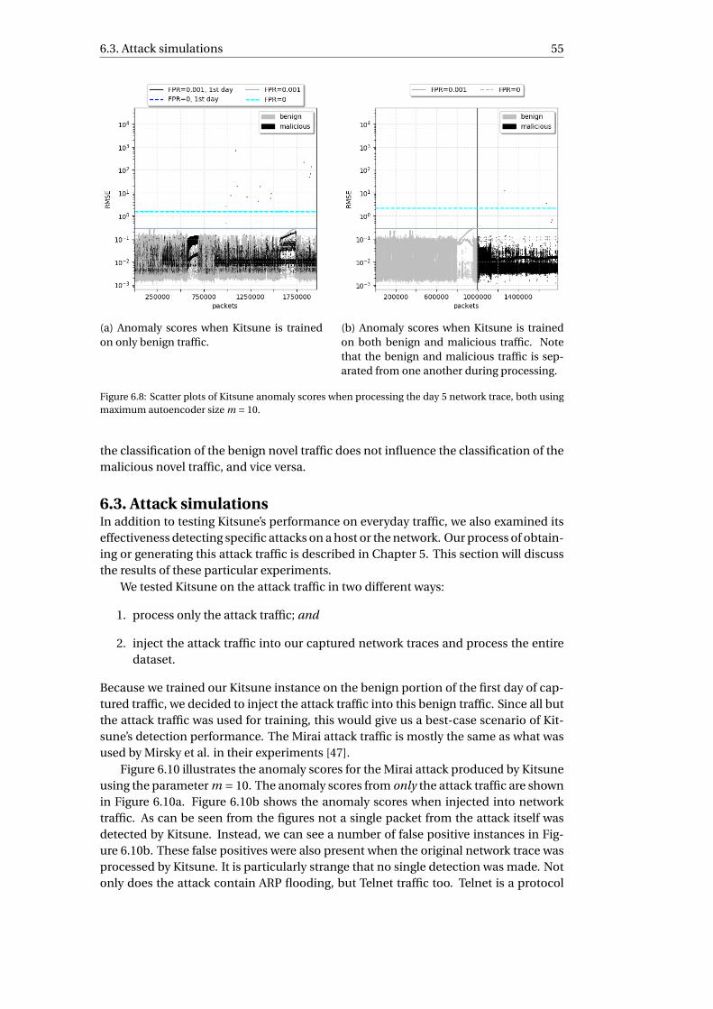
6.3. Attack simulations 55
(a) Anomaly scores when Kitsune is trainedon only benign traffic.
(b) Anomaly scores when Kitsune is trainedon both benign and malicious traffic. Notethat the benign and malicious traffic is sep-arated from one another during processing.
Figure 6.8: Scatter plots of Kitsune anomaly scores when processing the day 5 network trace, both usingmaximum autoencoder size m = 10.
the classification of the benign novel traffic does not influence the classification of themalicious novel traffic, and vice versa.
6.3. Attack simulationsIn addition to testing Kitsune’s performance on everyday traffic, we also examined itseffectiveness detecting specific attacks on a host or the network. Our process of obtain-ing or generating this attack traffic is described in Chapter 5. This section will discussthe results of these particular experiments.
We tested Kitsune on the attack traffic in two different ways:
1. process only the attack traffic; and
2. inject the attack traffic into our captured network traces and process the entiredataset.
Because we trained our Kitsune instance on the benign portion of the first day of cap-tured traffic, we decided to inject the attack traffic into this benign traffic. Since all butthe attack traffic was used for training, this would give us a best-case scenario of Kit-sune’s detection performance. The Mirai attack traffic is mostly the same as what wasused by Mirsky et al. in their experiments [47].
Figure 6.10 illustrates the anomaly scores for the Mirai attack produced by Kitsuneusing the parameter m = 10. The anomaly scores from only the attack traffic are shownin Figure 6.10a. Figure 6.10b shows the anomaly scores when injected into networktraffic. As can be seen from the figures not a single packet from the attack itself wasdetected by Kitsune. Instead, we can see a number of false positive instances in Fig-ure 6.10b. These false positives were also present when the original network trace wasprocessed by Kitsune. It is particularly strange that no single detection was made. Notonly does the attack contain ARP flooding, but Telnet traffic too. Telnet is a protocol
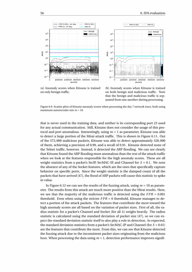
56 6. IDS evaluation
(a) Anomaly scores when Kitsune is trainedon only benign traffic.
(b) Anomaly scores when Kitsune is trainedon both benign and malicious traffic. Notethat the benign and malicious traffic is sep-arated from one another during processing.
Figure 6.9: Scatter plots of Kitsune anomaly scores when processing the day 7 network trace, both usingmaximum autoencoder size m = 10.
that is never used in the training data, and neither is its corresponding port 23 usedfor any actual communication. Still, Kitsune does not consider the usage of this pro-tocol and port anomalous. Interestingly, using m = 1 as parameter, Kitsune was ableto detect a large portion of the Mirai attack traffic. This is shown in Figure 6.11. Outof the 575,000 malicious packets, Kitsune was able to detect approximately 520,000of them, achieving a precision of 0.99, and a recall of 0.91. Kitsune detected none ofthe Telnet traffic, however. Instead, it detected the ARP flooding. We can see clearlythat Kitsune found the ARP flooding more anomalous than the rest of the attack trafficwhen we look at the features responsible for the high anomaly scores. These are allweight statistics from a packet’s SrcIP, SrcMAC-IP, and Channel for λ = 0.1. We notethe absence of any of the Socket features, which are the ones that specifically capturebehavior on specific ports. Since the weight statistic is the damped count of all thepackets that have arrived [47], the flood of ARP packets will cause this statistic to spikein value.
In Figure 6.12 we can see the results of the fuzzing attack, using m = 10 as param-eter. The results from this attack are much more positive than the Mirai results. Here,we see that the majority of the malicious traffic is detected using the F PR = 0.001threshold. Even when using the stricter F PR = 0 threshold, Kitsune manages to de-tect a portion of the attack packets. The features that contribute the most toward thehigh anomaly scores are all based on the variation of packet sizes. First of all, the ra-dius statistic for a packet’s Channel and Socket (for all λ) weighs heavily. The radiusstatistic is calculated using the standard deviation of packet size [47], so we can ex-pect the standard deviation statistic itself to also play a role in detection. As expected,the standard deviation statistics from a packet’s SrcMAC-IP and Channel (for λ= 0.01)are the features that contribute the most. From this, we can see that Kitsune detectedthe fuzzing attack due to the inconsistent packet sizes originating from the malicioushost. When processing the data using m = 1, detection performance improves signifi-
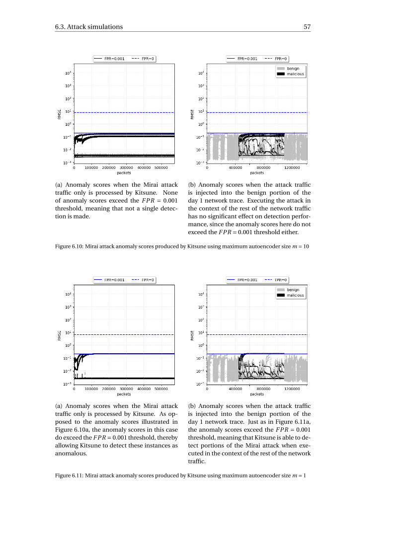
6.3. Attack simulations 57
(a) Anomaly scores when the Mirai attacktraffic only is processed by Kitsune. Noneof anomaly scores exceed the F PR = 0.001threshold, meaning that not a single detec-tion is made.
(b) Anomaly scores when the attack trafficis injected into the benign portion of theday 1 network trace. Executing the attack inthe context of the rest of the network traffichas no significant effect on detection perfor-mance, since the anomaly scores here do notexceed the F PR = 0.001 threshold either.
Figure 6.10: Mirai attack anomaly scores produced by Kitsune using maximum autoencoder size m = 10
(a) Anomaly scores when the Mirai attacktraffic only is processed by Kitsune. As op-posed to the anomaly scores illustrated inFigure 6.10a, the anomaly scores in this casedo exceed the F PR = 0.001 threshold, therebyallowing Kitsune to detect these instances asanomalous.
(b) Anomaly scores when the attack trafficis injected into the benign portion of theday 1 network trace. Just as in Figure 6.11a,the anomaly scores exceed the F PR = 0.001threshold, meaning that Kitsune is able to de-tect portions of the Mirai attack when exe-cuted in the context of the rest of the networktraffic.
Figure 6.11: Mirai attack anomaly scores produced by Kitsune using maximum autoencoder size m = 1
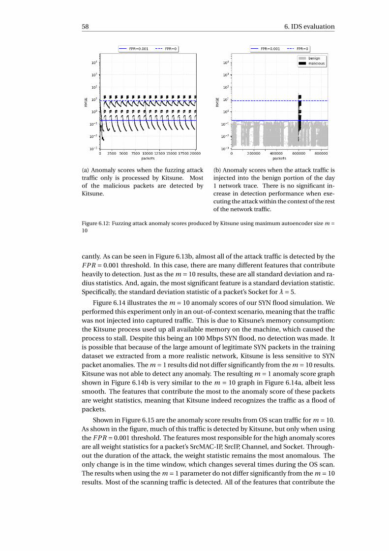
58 6. IDS evaluation
(a) Anomaly scores when the fuzzing attacktraffic only is processed by Kitsune. Mostof the malicious packets are detected byKitsune.
(b) Anomaly scores when the attack traffic isinjected into the benign portion of the day1 network trace. There is no significant in-crease in detection performance when exe-cuting the attack within the context of the restof the network traffic.
Figure 6.12: Fuzzing attack anomaly scores produced by Kitsune using maximum autoencoder size m =10
cantly. As can be seen in Figure 6.13b, almost all of the attack traffic is detected by theF PR = 0.001 threshold. In this case, there are many different features that contributeheavily to detection. Just as the m = 10 results, these are all standard deviation and ra-dius statistics. And, again, the most significant feature is a standard deviation statistic.Specifically, the standard deviation statistic of a packet’s Socket for λ= 5.
Figure 6.14 illustrates the m = 10 anomaly scores of our SYN flood simulation. Weperformed this experiment only in an out-of-context scenario, meaning that the trafficwas not injected into captured traffic. This is due to Kitsune’s memory consumption:the Kitsune process used up all available memory on the machine, which caused theprocess to stall. Despite this being an 100 Mbps SYN flood, no detection was made. Itis possible that because of the large amount of legitimate SYN packets in the trainingdataset we extracted from a more realistic network, Kitsune is less sensitive to SYNpacket anomalies. The m = 1 results did not differ significantly from the m = 10 results.Kitsune was not able to detect any anomaly. The resulting m = 1 anomaly score graphshown in Figure 6.14b is very similar to the m = 10 graph in Figure 6.14a, albeit lesssmooth. The features that contribute the most to the anomaly score of these packetsare weight statistics, meaning that Kitsune indeed recognizes the traffic as a flood ofpackets.
Shown in Figure 6.15 are the anomaly score results from OS scan traffic for m = 10.As shown in the figure, much of this traffic is detected by Kitsune, but only when usingthe F PR = 0.001 threshold. The features most responsible for the high anomaly scoresare all weight statistics for a packet’s SrcMAC-IP, SrcIP, Channel, and Socket. Through-out the duration of the attack, the weight statistic remains the most anomalous. Theonly change is in the time window, which changes several times during the OS scan.The results when using the m = 1 parameter do not differ significantly from the m = 10results. Most of the scanning traffic is detected. All of the features that contribute the
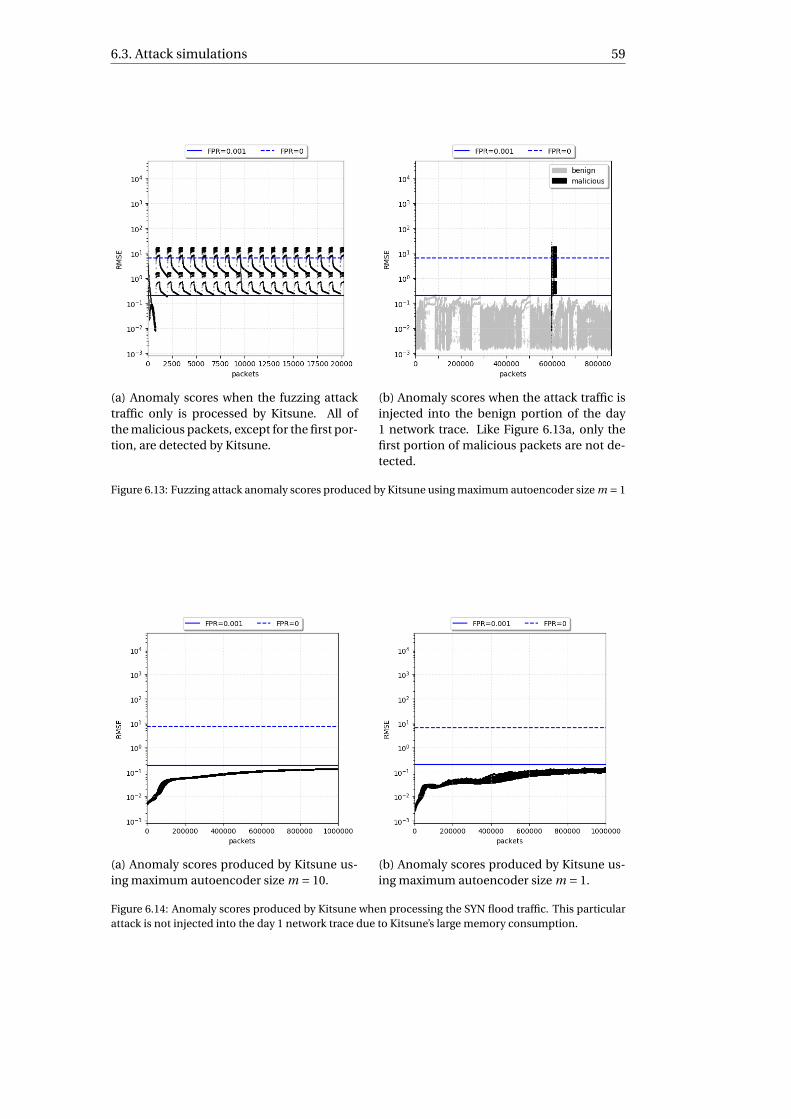
6.3. Attack simulations 59
(a) Anomaly scores when the fuzzing attacktraffic only is processed by Kitsune. All ofthe malicious packets, except for the first por-tion, are detected by Kitsune.
(b) Anomaly scores when the attack traffic isinjected into the benign portion of the day1 network trace. Like Figure 6.13a, only thefirst portion of malicious packets are not de-tected.
Figure 6.13: Fuzzing attack anomaly scores produced by Kitsune using maximum autoencoder size m = 1
(a) Anomaly scores produced by Kitsune us-ing maximum autoencoder size m = 10.
(b) Anomaly scores produced by Kitsune us-ing maximum autoencoder size m = 1.
Figure 6.14: Anomaly scores produced by Kitsune when processing the SYN flood traffic. This particularattack is not injected into the day 1 network trace due to Kitsune’s large memory consumption.

60 6. IDS evaluation
(a) Anomaly scores when the fuzzing attacktraffic only is processed by Kitsune.
(b) Anomaly scores when the OS scan trafficis injected into the benign portion of the day1 network trace. There is no improvement indetection performance.
Figure 6.15: OS scan anomaly scores produced by Kitsune using maximum autoencoder size m = 10
most toward the high anomaly scores are weight statistics, mostly for the Socket be-tween the scanning host and the host being scanned.
The m = 10 results from the successful SSH brute-force attack are shown in Fig-ure 6.16. As can be seen, the actual brute-force traffic that makes up the majority ofthe malicious traffic is not detected by Kitsune. Kitsune was only able to detect threepackets at the very end of the attack. The detected packets contain a command sentto the victim’s machine, and the victim’s response after successfully guessing the pass-word and logging in. These packets are larger than the ones sent during the brute-force attack, and this is precisely the reason why Kitsune was able to detect them. Wecan see this when looking at the responsible features, as they are all standard devia-tion statistics for a packet’s SrcMAC-IP, SrcIP, Channel, and Socket, for several differenttime windows λ. For m = 1, the feature most responsible for detection is also a stan-dard deviation statistic: the standard deviation in packet size for the Socket betweenthe attacker and victim for λ= 5. This means that for both cases, the change in packetsize is responsible for the detection of these last few attack packets.
Figure 6.17 illustrates the anomaly scores of the DNS abuse traffic using the m = 10Kitsune instance. The version of the attack with 100 incoming DNS queries per mil-lisecond is shown in Figures 6.17a and 6.17b, while the version with one query permillisecond is shown in Figures 6.17c and 6.17d. In the figures belonging to the attacktraffic-only anomaly scores (Figures 6.17a and 6.17c), we clearly see that the graphscontain two separate curves. One of the curves represents the anomaly scores of theincoming DNS queries, while the other represents the anomaly scores of the outgo-ing DNS responses. Compared to the SYN flood attack, this attack contains muchless packets, and the speed at which the packets arrive is also much slower. Despitethis, Kitsune is able to detect the attack in both circumstances with the F PR = 0.001threshold. Kitsune is much better able to detect the version of the attack with the fasterpacket rate. When we examine the feature cluster that is most responsible for the highanomaly scores, we can see why this is the case: all of the features in the cluster areweight statistics. The amount of packets that Kitsune receives within a certain time
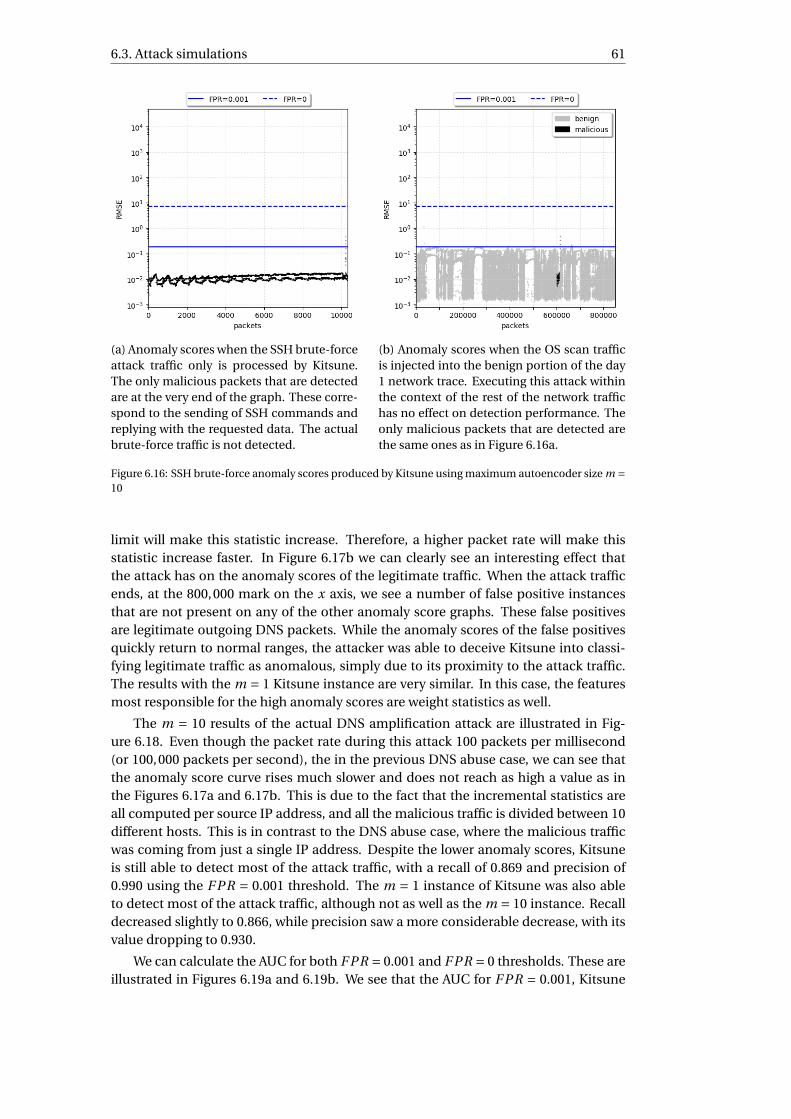
6.3. Attack simulations 61
(a) Anomaly scores when the SSH brute-forceattack traffic only is processed by Kitsune.The only malicious packets that are detectedare at the very end of the graph. These corre-spond to the sending of SSH commands andreplying with the requested data. The actualbrute-force traffic is not detected.
(b) Anomaly scores when the OS scan trafficis injected into the benign portion of the day1 network trace. Executing this attack withinthe context of the rest of the network traffichas no effect on detection performance. Theonly malicious packets that are detected arethe same ones as in Figure 6.16a.
Figure 6.16: SSH brute-force anomaly scores produced by Kitsune using maximum autoencoder size m =10
limit will make this statistic increase. Therefore, a higher packet rate will make thisstatistic increase faster. In Figure 6.17b we can clearly see an interesting effect thatthe attack has on the anomaly scores of the legitimate traffic. When the attack trafficends, at the 800,000 mark on the x axis, we see a number of false positive instancesthat are not present on any of the other anomaly score graphs. These false positivesare legitimate outgoing DNS packets. While the anomaly scores of the false positivesquickly return to normal ranges, the attacker was able to deceive Kitsune into classi-fying legitimate traffic as anomalous, simply due to its proximity to the attack traffic.The results with the m = 1 Kitsune instance are very similar. In this case, the featuresmost responsible for the high anomaly scores are weight statistics as well.
The m = 10 results of the actual DNS amplification attack are illustrated in Fig-ure 6.18. Even though the packet rate during this attack 100 packets per millisecond(or 100,000 packets per second), the in the previous DNS abuse case, we can see thatthe anomaly score curve rises much slower and does not reach as high a value as inthe Figures 6.17a and 6.17b. This is due to the fact that the incremental statistics areall computed per source IP address, and all the malicious traffic is divided between 10different hosts. This is in contrast to the DNS abuse case, where the malicious trafficwas coming from just a single IP address. Despite the lower anomaly scores, Kitsuneis still able to detect most of the attack traffic, with a recall of 0.869 and precision of0.990 using the F PR = 0.001 threshold. The m = 1 instance of Kitsune was also ableto detect most of the attack traffic, although not as well as the m = 10 instance. Recalldecreased slightly to 0.866, while precision saw a more considerable decrease, with itsvalue dropping to 0.930.
We can calculate the AUC for both F PR = 0.001 and F PR = 0 thresholds. These areillustrated in Figures 6.19a and 6.19b. We see that the AUC for F PR = 0.001, Kitsune
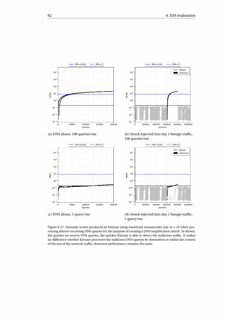
62 6. IDS evaluation
(a) DNS abuse, 100 queries/ms (b) Attack injected into day 1 benign traffic,100 queries/ms
(c) DNS abuse, 1 query/ms (d) Attack injected into day 1 benign traffic,1 query/ms
Figure 6.17: Anomaly scores produced by Kitsune using maximum autoencoder size m = 10 when pro-cessing abusive incoming DNS queries for the purpose of creating a DNS amplification attack. As shown,the quicker we receive DNS queries, the quicker Kitsune is able to detect the malicious traffic. It makesno difference whether Kitsune processes the malicious DNS queries by themselves or within the contextof the rest of the network traffic; detection performance remains the same.
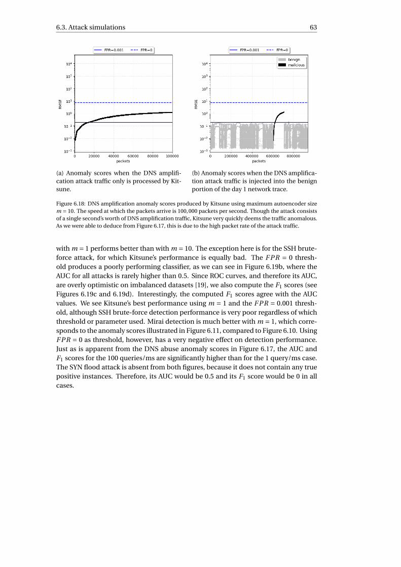
6.3. Attack simulations 63
(a) Anomaly scores when the DNS amplifi-cation attack traffic only is processed by Kit-sune.
(b) Anomaly scores when the DNS amplifica-tion attack traffic is injected into the benignportion of the day 1 network trace.
Figure 6.18: DNS amplification anomaly scores produced by Kitsune using maximum autoencoder sizem = 10. The speed at which the packets arrive is 100,000 packets per second. Though the attack consistsof a single second’s worth of DNS amplification traffic, Kitsune very quickly deems the traffic anomalous.As we were able to deduce from Figure 6.17, this is due to the high packet rate of the attack traffic.
with m = 1 performs better than with m = 10. The exception here is for the SSH brute-force attack, for which Kitsune’s performance is equally bad. The F PR = 0 thresh-old produces a poorly performing classifier, as we can see in Figure 6.19b, where theAUC for all attacks is rarely higher than 0.5. Since ROC curves, and therefore its AUC,are overly optimistic on imbalanced datasets [19], we also compute the F1 scores (seeFigures 6.19c and 6.19d). Interestingly, the computed F1 scores agree with the AUCvalues. We see Kitsune’s best performance using m = 1 and the F PR = 0.001 thresh-old, although SSH brute-force detection performance is very poor regardless of whichthreshold or parameter used. Mirai detection is much better with m = 1, which corre-sponds to the anomaly scores illustrated in Figure 6.11, compared to Figure 6.10. UsingF PR = 0 as threshold, however, has a very negative effect on detection performance.Just as is apparent from the DNS abuse anomaly scores in Figure 6.17, the AUC andF1 scores for the 100 queries/ms are significantly higher than for the 1 query/ms case.The SYN flood attack is absent from both figures, because it does not contain any truepositive instances. Therefore, its AUC would be 0.5 and its F1 score would be 0 in allcases.
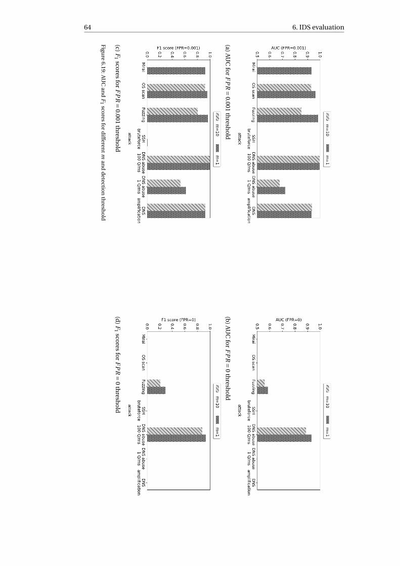
64 6. IDS evaluation
(a)A
UC
for
FP
R=
0.001th
resho
ld(b
)A
UC
for
FP
R=
0th
resho
ld
(c)F
1sco
resfo
rF
PR=
0.001th
resho
ld(d
)F
1sco
resfo
rF
PR=
0th
resho
ld
Figu
re6.19:A
UC
and
F1
scores
for
differen
tman
dd
etection
thresh
old
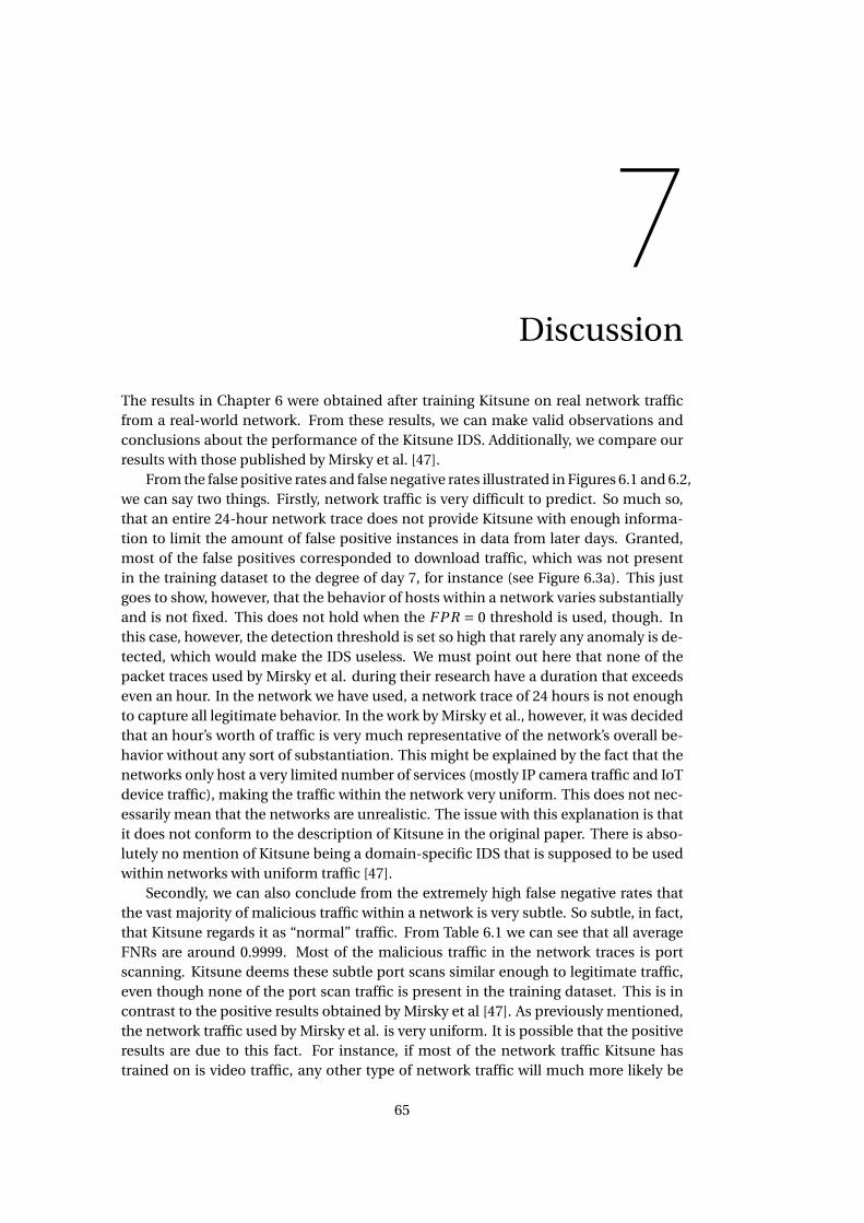
7Discussion
The results in Chapter 6 were obtained after training Kitsune on real network trafficfrom a real-world network. From these results, we can make valid observations andconclusions about the performance of the Kitsune IDS. Additionally, we compare ourresults with those published by Mirsky et al. [47].
From the false positive rates and false negative rates illustrated in Figures 6.1 and 6.2,we can say two things. Firstly, network traffic is very difficult to predict. So much so,that an entire 24-hour network trace does not provide Kitsune with enough informa-tion to limit the amount of false positive instances in data from later days. Granted,most of the false positives corresponded to download traffic, which was not presentin the training dataset to the degree of day 7, for instance (see Figure 6.3a). This justgoes to show, however, that the behavior of hosts within a network varies substantiallyand is not fixed. This does not hold when the F PR = 0 threshold is used, though. Inthis case, however, the detection threshold is set so high that rarely any anomaly is de-tected, which would make the IDS useless. We must point out here that none of thepacket traces used by Mirsky et al. during their research have a duration that exceedseven an hour. In the network we have used, a network trace of 24 hours is not enoughto capture all legitimate behavior. In the work by Mirsky et al., however, it was decidedthat an hour’s worth of traffic is very much representative of the network’s overall be-havior without any sort of substantiation. This might be explained by the fact that thenetworks only host a very limited number of services (mostly IP camera traffic and IoTdevice traffic), making the traffic within the network very uniform. This does not nec-essarily mean that the networks are unrealistic. The issue with this explanation is thatit does not conform to the description of Kitsune in the original paper. There is abso-lutely no mention of Kitsune being a domain-specific IDS that is supposed to be usedwithin networks with uniform traffic [47].
Secondly, we can also conclude from the extremely high false negative rates thatthe vast majority of malicious traffic within a network is very subtle. So subtle, in fact,that Kitsune regards it as “normal” traffic. From Table 6.1 we can see that all averageFNRs are around 0.9999. Most of the malicious traffic in the network traces is portscanning. Kitsune deems these subtle port scans similar enough to legitimate traffic,even though none of the port scan traffic is present in the training dataset. This is incontrast to the positive results obtained by Mirsky et al [47]. As previously mentioned,the network traffic used by Mirsky et al. is very uniform. It is possible that the positiveresults are due to this fact. For instance, if most of the network traffic Kitsune hastrained on is video traffic, any other type of network traffic will much more likely be
65
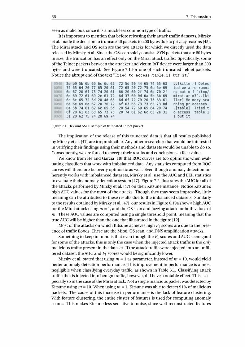
66 7. Discussion
seen as malicious, since it is a much less common type of traffic.It is important to mention that before releasing their attack traffic datasets, Mirsky
et al. made the decision to truncate all packets to 200 bytes due to privacy reasons [45].The Mirai attack and OS scan are the two attacks for which we directly used the datareleased by Mirsky et al. Since the OS scan solely consists SYN packets that are 60 bytesin size, the truncation has an effect only on the Mirai attack traffic. Specifically, someof the Telnet packets between the attacker and victim IoT device were larger than 200bytes and were truncated. See Figure 7.1 for one of such truncated Telnet packets.Notice the abrupt end of the text “Tried to access table.11 but it.”
Figure 7.1: Hex and ASCII sample of truncated Telnet packet
The implication of the release of this truncated data is that all results publishedby Mirsky et al. [47] are irreproducible. Any other researcher that would be interestedin verifying their findings using their methods and datasets would be unable to do so.Consequently, we are forced to accept their results and conclusions at face value.
We know from He and Garcia [19] that ROC curves are too optimistic when eval-uating classifiers that work with imbalanced data. Any statistics computed from ROCcurves will therefore be overly optimistic as well. Even though anomaly detection in-herently works with imbalanced datasets, Mirsky et al. use the AUC and EER statisticsto evaluate their anomaly detection system [47]. Figure 7.2 illustrates the AUC for all ofthe attacks performed by Mirsky et al. [47] on their Kitsune instance. Notice Kitsune’shigh AUC values for the most of the attacks. Though they may seem impressive, littlemeaning can be attributed to these results due to the imbalanced datasets. Similarlyto the results obtained by Mirsky et al. [47], our results in Figure 6.19a show a high AUCfor the Mirai attack using m = 1, and the OS scan and fuzzing attack for both values ofm. These AUC values are computed using a single threshold point, meaning that thetrue AUC will be higher than the one that illustrated in the figure [12].
Most of the attacks on which Kitsune achieves high F1 scores are due to the pres-ence of traffic floods. These are the Mirai, OS scan, and DNS amplification attacks.
Something to keep in mind is that even though the F1 scores and AUC seem goodfor some of the attacks, this is only the case when the injected attack traffic is the onlymalicious traffic present in the dataset. If the attack traffic were injected into an unfil-tered dataset, the AUC and F1 scores would be significantly lower.
Mirsky et al. stated that using m = 1 as parameter, instead of m = 10, would yieldbetter anomaly detection performance. This improvement in performance is almostnegligible when classifying everyday traffic, as shown in Table 6.1. Classifying attacktraffic that is injected into benign traffic, however, did have a notable effect. This is es-pecially so in the case of the Mirai attack. Not a single malicious packet was detected byKitsune using m = 10. When using m = 1, Kitsune was able to detect 91% of maliciouspackets. The cause of this increase in performance is the lack of feature clustering.With feature clustering, the entire cluster of features is used for computing anomalyscores. This makes Kitsune less sensitive to noise, since well-reconstructed features

67
Figure 7.2: AUC values for the attacks performed by Mirsky et al. [47]
in the cluster will compensate for the single anomalous feature that would otherwisecause a large RMSE. There is a side effect to this, though. Using m = 1, clusters containat most a single feature, meaning that there are no other features in the cluster thatcan compensate for a single anomalous feature. This can amplify the final anomalyscore that is computed for a particular packet, especially if the anomalous features arereconstructed particularly poorly.
Given the anomalies that were successfully detected, it seems that Kitsune specifi-cally looks out for two types of behavior:
1. sudden surges of traffic with little delay between each packet; and
2. inconsistencies in the amount of data exchanged between hosts.
These inconsistencies can be abnormally large packets coming from a certain host, asin the fuzzing attack, or an imbalance between the amount of data sent and received,as in the case illustrated in Figures 6.5 and 6.6. If we look at the design of the KitsuneIDS, we see that all features are computed using only packet counts, packet sizes andpacket timestamps. Therefore, it makes sense that Kitsune would look out for the twoaforementioned behaviors. No special attention is paid to the content of a packet’spayload. Take the cases of the Mirai attack and OS scan, for instance. The detec-tion of all malicious packets was based entirely on packet counts within a certain timewindow. While detecting the Mirai attack’s ARP flood using packet counts is under-standable, detection of the OS scan can be easily circumvented by limiting the speedat which the adversary sends out SYN packets. The processing of both versions of theDNS abuse cases also exemplifies Kitsune’s preference for detecting sudden surges intraffic. We can see the attack with the higher packet rate produces high anomaly scoresmuch faster than the attack with the slower packet rate. The DNS abuse traffic andDNS amplification attack also demonstrate the significance of the origin of a trafficflood. If, for a certain packet rate, all network traffic originates from a single IP address,Kitsune will more readily classify the flood as anomalous. Given that same packet rate,Kitsune will find it increasingly difficult to detect the flood as the number of partici-pants in the flood attack increase. For example, if a botnet contains enough hosts, it
68 7. Discussion
is certainly possible that Kitsune will not be able to detect a DDoS attack initiated bythat botnet if every host limits its packet rate properly.
In the cases of the fuzzing attack and SSH brute-force, the packets were detectedby looking at the variation in the sizes of packets sent between two hosts. The SSHbrute-force provides the clearest example of this. Most of the packets in the attack areunder 200 bytes, which correspond to the login attempts. None of these packets areseen as malicious. It took just a single packet with a size of 3262 bytes sent betweenthe hosts for the anomaly scores to spike. After this packet, the anomaly scores quicklyreturn to the “normal” range. Thus, detection can be avoided by ensuring packet sizesdo not exceed a certain size.
Though Kitsune was unable to make a single detection during the SYN flood, thecurves illustrated in Figure 6.14 seem to have positive slopes. Given a larger SYN flooddataset, and a machine with the resources necessary to process it, the anomaly scoresmight eventually cross the F PR = 0.001 threshold. Just like this SYN flood, the OS scanis composed of only SYN packets. The only difference is that the SYN flood is directedat a single port, while the OS scan send out SYN packets to a large range of ports. Seeingthat much of the OS scan was detected (see Figure 6.15), it is entirely possible that aSYN flood would be detected, given a larger dataset.
The fact that Kitsune does not take the payload into account when analyzing apacket is a serious drawback. Especially in larger networks, packets of all sizes canbe found, meaning that packet size loses its value as a metric. Additionally, maliciouspackets can be crafted that are as large (or as small) as legitimate packets. Take Heart-bleed packets, for instance, which are 74 bytes in size. It is certainly not uncommon tosee legitimate SSH packets of that size (or legitimate heartbeat packets, for that mat-ter). Malicious Heartbleed packets could erroneously be lumped together with legiti-mate traffic, simply because the packet is of a normal size.
With the results we obtained from our experiments, we have demonstrated twothings. Firstly, we have found that when deploying Kitsune in a real-world environ-ment and training it on real-world data, it is utterly ineffective as an IDS. It is veryrarely able to detect malicious traffic, and its false positive rate is much to high for itto be useful in practice. Our network received an average of 690 MB of network trafficper day. Using the better-performing m = 1 version of Kitsune with the F PR = 0.001threshold, Kitsune would flag 39 MB worth of packets as anomalies per day. Secondly,we have shown that Kitsune is only able to reliably detect malicious packets that areeither too large or arrive to quickly one after the other (e.g. a DDoS attack). Detec-tion of specific attacks can be evaded without much difficulty if the attacker knows thenormal behavior of the network. This makes Kitsune essentially no more than a DoSor packet flood detector, as opposed to a general anomaly detection system.
These findings can be condensed into the following statement: flawed methodslead to flawed results. It is very likely that the authors could have spotted their er-rors if they ensured the data and methodology they used were valid. In fact, suchmistakes could have been avoided in the first place. From the results obtained fromthis case study, as well as the numerous other IDS papers discussed in Chapter 2, it isapparent that usage of flawed data and methods are widespread. IDSs are thus eval-uated in an incorrect manner, unfortunately leading to the generation of potentiallyerroneous information. Additionally, not every team of researchers uses the same pro-cesses when implementing and evaluating their designed IDS. This emphasizes thenecessity for a set methodology that is designed to ensure proper evaluation of an IDS.For instance, many different authors often do not even use the same datasets when
69
evaluating an IDS. On top of that, much of this data is flawed in some way, it beingeither unrealistic simulated data, or data extracted from an unrealistic or artificial net-work [36, 40, 73, 80]. The “gold standard” is network traffic that is extracted from areal-world network that is as large as one can get their hands on [73]. An issue withcollecting real traffic is that none of it will be labeled. Since labeling is important formachine learning, it is necessary to engage in some form of collaboration with the ad-ministrator of the network in order to label the traffic accurately and extract the neces-sary ground-truth for classification. Of course, this is a time-consuming process, butthere certainly is payoff in the form the ability to perform of valid experiments. Thisin turn leads to valid results. Finally, the evaluation process needs to be appropriatefor the field of anomaly detection. Basing conclusions on different overly optimistic oruninformative metrics (e.g. ROC curves, accuracy) will also stand in the way valid eval-uations and conclusions [19]. Agreeing on a common design and evaluation processwould help researchers create valid research. Furthermore, such a common processwill also allow for the easier reproduction of research by others, thereby helping theanomaly detection community as a whole as well. The steps that we have followed inour case study are extracted from academic literature. These steps can be aggregatedand formalized to create a framework that is easy to follow and makes research morerepeatable. This framework is presented in Section 8.3


8Conclusion
Machine learning-based anomaly detection is a heavily studied field of research. Manyresearchers develop their own system using different techniques and evaluation meth-ods. According to Sommer and Paxson [73], much of these methodologies are not suit-able for the proper design and evaluation of intrusion detection systems. Other re-searchers will readily consider this previous research as flawless and completely truth-ful, and build their research upon this faulty foundation. To our knowledge, none ofthis research has been revisited in order to validate the findings. Neither have therebeen independent reviews that aim to replicate the results. It was for these reasonsthat we considered it an interesting endeavor attempting to do precisely that.
In our research, we selected one specific machine learning-based IDS that wastrained and evaluated using network traffic from small and unrealistic networks. Muchof this network traffic was very uniform and contained hardly any noise. With the workwe performed, we have successfully demonstrated this observation. Specifically, wehave shown that training and deploying a machine learning-based IDS in a real-worldscenario will yield wildly different results compared to an artificial or unrealistic sce-nario. Real-world networks are busier and noisier than private or artificial networks.Undoubtedly, this fact will have a considerable effect on the performance of any suchIDS. In this chapter, we come back to our main research question:
How can a machine learning-based intrusion detection system be correctly evaluated?
This chapter will elaborate on how we provided an answer to this question andhow our research objective was achieved. Due to time constraints, we were only ableto perform a single case study, using a single IDS for this project. This opens up severalpaths for future research, which will also be discussed in this chapter. Finally, we willpresent CAML-IDS, a framework that combines the best practices for anomaly detec-tion research that we have discovered during our work on this project, which will allowfor the correct assessment of machine learning-based intrusion detection systems.
8.1. Research objectiveBy combining the thorough literature analysis with the results obtained from our re-search itself, we are able to answer all of the sub-questions mentioned in Chapter 1.However, due to time constraints, we have only been able to propose a possible an-swer to our original research question. Several additional steps are necessary in or-der to provide a definitive answer to the research question. These will be discussed
71
72 8. Conclusion
in Section 8.2, where we discuss possible future work. Below we will discuss the sub-questions that we were able to answer.
Firstly, properly collecting data for a machine learning-based IDS requires the cap-ture of real network traffic from a real-world network. This network is preferably aslarge as possible. Or rather, as large a network as one can get access to. Also, a suffi-cient amount of network traffic needs to be captured. This is important, because smallnetwork traces will not contain enough of the network traffic to adequately model thenetwork’s behavior.
In order to annotate the anomalous data correctly, we need a comprehensive de-scription of the network from which the traffic is being captured. The description ofthe network is compiled by the administrator of the network, and, if necessary, is it-eratively improved through cooperation between the researcher and administrator. Acomplete network description allows for the establishing of ground-truth, which is acrucial aspect of anomaly detection. By establishing ground-truth for the captureddata, we can determine which data is benign and which is anomalous with absolutecertainty.
When evaluating the IDS on attack traffic, we have to ensure that the injected at-tack traffic closely matches the actual traffic that is found within the network. If theattack traffic is simulated, or the attack was originally performed on different hosts,the traffic needs to be altered. Otherwise, these differences might influence the per-formance of the IDS, thereby invalidating any results that are obtained. For example,IP and MAC addresses need to be changed to ones that match the network.
Finally, the evaluation metrics that are used must be appropriate for the field ofanomaly detection. Instead of simply using detection accuracy as a metric, precisionand recall should be used, because these take false positive instances into account.Moreover, instead of the widely-used ROC curve, precision-recall (PR) curve should beused, since ROC curves are very optimistic when dealing with imbalanced datasets. Inthe case that a single value is desired that describes the performance of an anomaly-based IDS, the F1 score can be computed as well.
By combining the aforementioned guidelines into a usable assessment framework,we provide a possible solution to the problem of properly evaluating the performanceof machine learning-based intrusion detection systems. This framework still needsfurther research, and this will be elaborated upon in the next section.
8.2. Future workOur work collects the best practices from across this field of research and combinesthem to form our proposed framework. The next step in this process is to evaluate theframework itself, which will provide definitive proof about its usefulness.
8.2.1. Evaluation of the frameworkBy applying this framework and to work by Mirsky et al. [47], this project demonstratesthe failings in current anomaly detection research. However, even though this researchdemonstrates shortcomings in current research, the fact remains that this case studyconsiders only a single IDS. There are many more anomaly-based IDS papers that canbe revisited. By revisiting such previous research and reproducing it using the frame-work we have proposed, we can gain more insight into the validity of the framework.A key aspect of any academic studies is its reproducibility. Therefore, it is necessaryto, not only test IDSs using this same framework, but also using the same data thatwas used in this study. This ensures that the only variable in the future experiments
8.2. Future work 73
is the IDS itself. If further research demonstrates the validity of this framework, then,naturally, a good way forward is to adhere to our proposed framework when workingon anomaly detection research in the future. Doing so would prevent researchers frommaking the errors that are so widespread in anomaly detection nowadays.
8.2.2. Revisiting previous researchRevisiting previous research is not only necessary for the evaluation of the framework,but it is also an opportunity to assess the validity of the research itself. More case stud-ies such as this are necessary to make definitive conclusions about the entire field ofresearch. As more of the research in this field is repeated using appropriate data andcorrect evaluation, more information will be available about the true state of anomalydetection research. Also, these repeats of existing research can be compiled together.Such a compilation of different case studies will researchers to better critique the fieldof anomaly detection.
8.2.3. Real-world testingLastly, it is certainly interesting to compare the steps as stated in this framework withthe processes that are followed when implementing an IDS in a real-world scenario.This comparison can also be used to see whether this framework is appropriate forpractical use. Sommer and Paxson [73] state that the most convincing evidence forthe value and usefulness of an IDS is to get feedback network operators who have im-plemented said system in their network. This same statement can be applied to thisframework. If network operators deem this framework useful for successfully imple-menting an effective IDS into their network, then it stands to reason that the frame-work certainly has value for both academic and practical use.

74 8. Conclusion
8.3. CAML-IDS
STEP ACTION REMARKS
1 Obtain access to a real-world net-work.
It is important that this network be aslarge possible
2 Obtain a detailed network descriptionfrom network administrator.
3 Create a static rule-set from the net-work description.
4 Collect the necessary network traffic.
5 Filter the collected network traffic us-ing the static rule-set into (i) legiti-mate, (ii) illegitimate, and (iii) unclas-sified traffic.
Network traffic will be unclassified ifit is not covered by any rule.
6 Take a subset of the unclassified traf-fic from Step 5 and refine the staticrule-set by adding rules that cover theinstances in the subset.
This is done in cooperation with thenetwork administrator in order to de-termine with certainty whether thetraffic is legitimate or not. This is im-portant for establishing ground-truth.
7 Repeat Steps 5 and 6 until all unclas-sified traffic has been successfully an-notated.
8 Train the IDS on the ground-truth le-gitimate traffic obtained from Steps 5and 6.
9 Test the IDS using the entirety of legit-imate and illegitimate traffic.
If attack traffic is injected into thedataset, ensure that this attack trafficmatches the used network as closelyas possible (e.g. IP addresses, MACaddresses, used protocols).
10 Evaluate the IDS performance usingsuitable statistics (e.g. precision, re-call, PR curves, F1 score).

Bibliography
[1] M. Antonakakis, T. April, M. Bailey, M. Bernhard, E. Bursztein, J. Cochran, Z. Du-rumeric, J. Halderman, L. Invernizzi, M. Kallitsis, et al. Understanding the MiraiBotnet. In Proc. Usenix Security Symp., pages 1092–1110, 2017.
[2] ASHRAE. BACnet/IP. http://www.bacnet.org/Tutorial/BACnetIP/sld004.html. Accessed on 6/2/2019.
[3] S. Axelsson. The Base-Rate Fallacy and Its Implications for the Difficulty of In-trusion Detection. In Proc. ACM Conference on Computer and CommunicationsSecurity (CCS), pages 1–7. ACM, 1999. ISBN 1-58113-148-8.
[4] W.J. Bloem. Sluizen, gemalen en bruggen slecht beveiligd. https://eenvandaag.avrotros.nl/binnenland/item/sluizen-gemalen-en-bruggen-slecht-beveiligd/, 2012. Accessed on 26/2/2018.
[5] D. Bolzoni, S. Etalle, and P. Hartel. Poseidon: A 2-Tier Anomaly-Based NetworkIntrusion Detection System. In Proc. IEEE International Workshop on InformationAssurance (IWIA), pages 144–156. IEEE, 2006. ISBN 0-7695-2564-4.
[6] T. Bradley. Pros and Cons of Bringing Your Own De-vice to Work. https://www.pcworld.com/article/246760/pros_and_cons_of_byod_bring_your_own_device_.html. Accessed on2/11/2018.
[7] CERT Division. 1996 CERT Advisories. https://resources.sei.cmu.edu/asset_files/WhitePaper/1996_019_001_496172.pdf. Accessed on1/20/2019.
[8] Cloudfare. DNS Amplification Attack. https://www.cloudflare.com/learning/ddos/dns-amplification-ddos-attack/, . Accessed on 6/3/2019.
[9] Cloudfare. Ping of Death DDoS attack. https://www.cloudflare.com/learning/ddos/ping-of-death-ddos-attack/, . Accessed on 3/1/2019.
[10] A. Conole. sfuzz | Penetration Testing Tools. https://tools.kali.org/vulnerability-analysis/sfuzz. Accessed on 20/11/2018.
[11] S.E. Coull, C.V. Wright, F. Monrose, M.P. Collins, M.K. Reiter, et al. Playing Devil’sAdvocate: Inferring Sensitive Information from Anonymized Network Traces. InProc. Internet Society Symposium on Network and Distributed System Security(NDSS), volume 7, pages 35–47, 2007.
[12] E.R. DeLong, D.M. DeLong, and D.L. Clarke-Pearson. Comparing the Areas UnderTwo or More Correlated Receiver Operating Characteristic Curves: A Nonpara-metric Approach. Biometrics, 44(3):837–845, 1988.
75
76 Bibliography
[13] O. Depren, M. Topallar, E. Anarim, and M.K. Ciliz. An Intelligent Intrusion De-tection System (IDS) for Anomaly and Misuse Detection in Computer Networks.Expert Systems with Applications, 29(4):713–722, 2005.
[14] J. Erickson. Hacking: The Art of Exploitation. No Starch Press, 2nd edition, 2008.ISBN 0132126958, 9780132126953.
[15] T. Fawcett. An Introduction to ROC Analysis. Pattern Recognition Letters, 27(8):861–874, 2006.
[16] C. Finseth. An Access Control Protocol, Sometimes Called TACACS. Technicalreport, 1993.
[17] J. Fogarty, R.S. Baker, and S.E. Hudson. Case Studies in the Use of ROC Curve Anal-ysis for Sensor-based Estimates in Human Computer Interaction. In Proc. Graph-ics Interface, pages 129–136. Canadian Human-Computer Communications Soci-ety, 2005. ISBN 1-56881-265-5.
[18] D. Greene, P. Cunningham, and R. Mayer. Unsupervised Learning and Cluster-ing. In Machine Learning Techniques for Multimedia, pages 51–90. Springer, 2008.ISBN 978-3-540-75171-7.
[19] H. He and E.A. Garcia. Learning from Imbalanced Data. IEEE Trans. on Knowledgeand Data Engineering (TKDE), (9):1263–1284, 2008.
[20] P. Hoffman. RFC 3207 - SMTP Service Extension for Secure SMTP over TransportLayer Security. RFC 3207, RFC Editor, February 2002. URL https://www.rfc-editor.org/rfc/rfc3207.txt.
[21] A. Huttunen, B. Swander, V. Volpe, L. DiBurro, and M. Stenberg. UDP Encapsula-tion of IPsec ESP Packets. Technical report, 2004.
[22] Imperva, Inc. The Top 10 DDoS Attack Trends. https://www.imperva.com/docs/DS_Incapsula_The_Top_10_DDoS_Attack_Trends_ebook.pdf. Ac-cessed on 6/3/2019.
[23] J.P. John, E. Katz-Bassett, A. Krishnamurthy, T. Anderson, and A. Venkataramani.Consensus Routing: The Internet as a Distributed System. In Proc. Usenix Sympo-sium on Networked Systems Design and Implementation (NSDI), pages 351–364,2008. ISBN 978-1-931971-58-4.
[24] E. Joyce. Malfunctioning sensor adds to list of problems at San Onofrenuclear power plant. https://www.scpr.org/news/2012/05/29/32601/malfunctioning-sensor-adding-list-things-wrong-san/, 2012. Accessedon 26/2/2018.
[25] J. Jylänki et al. juj/kNet. https://github.com/juj/kNet. Accessed on 6/2/2019.
[26] Kaspersky Lab. What is Smurf Attack? https://usa.kaspersky.com/resource-center/definitions/smurf-attack. Accessed on 3/1/2019.
[27] K.S. Killourhy and R.A. Maxion. Toward Realistic and Artifact-Free Insider-ThreatData. In Proc. Annual Computer Security Applications Conference (ACSAC), pages87–96. IEEE, 2007. ISBN 0-7695-3060-5.

Bibliography 77
[28] R. King. Researcher: U.S. Tops the World in Critical Infrastructure De-vices Connected to the Internet. https://blogs.wsj.com/cio/2014/10/08/researcher-u-s-tops-the-world-in-critical-infrastructure-devices-connected-to-the-internet/, 2014. Accessed on 20/2/2018.
[29] K. Labib and V.R. Vemuri. NSOM: A Tool to Detect Denial of Service Attacks UsingSelf-Organizing Maps. Technical report, 2002.
[30] K. Lakkaraju and A. Slagell. Evaluating the Utility of Anonymized Network Tracesfor Intrusion Detection. In Proc. International Conference on Security and Privacyin Communication Networks (SecureComm), page 17. ACM, 2008. ISBN 978-1-60558-241-2.
[31] Lincoln Laboratory, Massachusetts Institute of Technology. Datasets. https://www.ll.mit.edu/r-d/datasets. Accessed on 3/1/2019.
[32] C. Liou, J. Huang, and W. Yang. Modeling Word Perception Using the Elman Net-work. Neurocomputing, 71(16-18):3150–3157, 2008.
[33] R. Lippmann, R.K. Cunningham, D.J. Fried, I. Graf, K.R. Kendall, S.E. Webster, andM.A. Zissman. Results of the DARPA 1998 Offline Intrusion Detection Evaluation.In Proc. RAID Recent Advances in Intrusion Detection, volume 99, pages 829–835,1999.
[34] R.P. Lippmann, D.J. Fried, I. Graf, J.W. Haines, K.R. Kendall, D. McClung, D. Weber,S.E. Webster, D. Wyschogrod, R.K. Cunningham, et al. Evaluating Intrusion Detec-tion Systems: The 1998 DARPA Off-Line Intrusion Detection Evaluation. In Proc.DARPA Information Survivability Conference and Exposition (DISCEX), volume 2,pages 12–26. IEEE, 2000. ISBN 0769504906.
[35] F. Liu, K.M. Ting, and Z. Zhou. Isolation Forest. In Proc. IEEE International Confer-ence on Data Mining (ICDM), pages 413–422. IEEE, 2008. ISBN 978-0-7695-3502-9.
[36] M. Mahoney and P.K. Chan. An Analysis of the 1999 DARPA/Lincoln LaboratoryEvaluation Data for Network Anomaly Detection. In Proc. RAID Recent Advancesin Intrusion Detection, pages 220–237. Springer, 2003. ISBN 3-540-40878-9.
[37] Mail.Ru. ICQ Privacy Policy. https://privacy.icq.com/legal/privacypolicy/en, . Accessed on 2/11/2018.
[38] Mail.Ru. Secure video calls with end-to-end encryption in ICQ. https://icq.com/security-calls/en, . Accessed on 2/11/2018.
[39] S. McCanne. libpcap: An Architecture and Optimization Methodologfor Packet Capture. https://sharkfestus.wireshark.org/sharkfest.11/presentations/McCanne-Sharkfest’11_Keynote_Address.pdf. Accessed on7/10/2018.
[40] J. McHugh. Testing Intrusion Detection Systems: A Critique of the 1998 and 1999DARPA Intrusion Detection System Evaluations as Performed by Lincoln Labo-ratory. ACM Trans. on Information and System Security (TISSEC), 3(4):262–294,2000.
78 Bibliography
[41] P. Mell. Understanding Intrusion Detection Systems. In IS Management Hand-book, pages 409–418. Auerbach Publications, 2003. ISBN 978-0849315954.
[42] Microsoft. [MC-DPLHP]: DirectPlay 8 Protocol: Host and Port Enu-meration. https://msdn.microsoft.com/en-us/library/cc217240.aspx?f=255&MSPPError=-2147217396. Accessed on 6/2/2019.
[43] mIRC Co., Ltd. mIRC: Using SSL with mIRC. https://www.mirc.com/ssl.html.Accessed on 2/11/2018.
[44] Y. Mirsky. ymirsky/Kitsune-py: A network intrusion detection system based onincremental statistics (AfterImage) and an ensemble of autoencoders (KitNET).https://github.com/ymirsky/Kitsune-py. Accessed on 3/10/2018.
[45] Y. Mirsky, T. Doitshman, Y. Elovici, and A. Shabtai. Kitsune Datasets. https://drive.google.com/drive/folders/1kmoWY4poGWfmmVSdSu-r_3Vo84Tu4PyE.Accessed on 10/11/2018.
[46] Y. Mirsky, B. Shapira, L. Rokach, and Y. Elovici. pcstream: A Stream ClusteringAlgorithm for Dynamically Detecting and Managing Temporal Contexts. In Proc.Pacific-Asia Conference on Knowledge Discovery and Data Mining (PAKDD), pages119–133. Springer, 2015. ISBN 978-3-319-18031-1.
[47] Y. Mirsky, T. Doitshman, Y. Elovici, and A. Shabtai. Kitsune: An Ensemble of Au-toencoders for Online Network Intrusion Detection. Proc. Internet Society Sym-posium on Network and Distributed System Security (NDSS), 2018.
[48] S. Mukkamala, G. Janoski, and A. Sung. Intrusion Detection Using Neural Net-works and Support Vector Machines. In Proc. International Joint Conference onNeural Networks (IJCNN), volume 2, pages 1702–1707. IEEE, 2002.
[49] R.S. Naoum, N.A. Abid, and Z.N. Al-Sultani. An Enhanced Resilient Backprop-agation Artificial Neural Network for Intrusion Detection System. InternationalJournal of Computer Science and Network Security (IJCSNS), 12(3):11, 2012.
[50] Nmap. Nmap: the Network Mapper - Free Security Scanner. https://nmap.org/.Accessed on 30/1/2019.
[51] Omron Europe B.V. FINS Commands Reference Manual.https://www.myomron.com/downloads/1.Manuals/Networks/W227E12_FINS_Commands_Reference_Manual.pdf. Accessed on 6/2/2019.
[52] OpenBSD. OpenBSD. https://www.openbsd.org/. Accessed on 2/11/2018.
[53] OpenSSH. sshd(8) - OpenBSD manual pages. https://man.openbsd.org/sshd.Accessed on 2/11/2018.
[54] K. Packard. X Display Manager Control Protocol. ftp://www.x.org/pub/X11R7.6/doc/libXdmcp/xdmcp.html. Accessed on 6/2/2019.
[55] A. Palczewska, J. Palczewski, R.M. Robinson, and D. Neagu. Interpreting RandomForest Classification Models Using a Feature Contribution Method. In Integrationof Reusable Systems, pages 193–218. Springer, 2014. ISBN 978-3-319-04717-1.

Bibliography 79
[56] R. Pang, M. Allman, V. Paxson, and J. Lee. The Devil and Packet Trace Anonymiza-tion. ACM Computer Communication Review (CCR), 36(1):29–38, 2006.
[57] I. Paul. 70-plus XMPP messaging services now securing chats with TLS encryp-tion. https://www.pcworld.com/article/2157180/xmpp-services-push-encrypted-connections-by-default.html. Accessed on 2/11/2018.
[58] J. Postel. Internet Control Message Protocol. RFC 792, RFC Editor, September1981. URL https://www.rfc-editor.org/rfc/pdfrfc/rfc792.txt.pdf.
[59] J. Postel. Transmission Control Protocol. RFC 793, RFC Editor, September 1981.URL https://www.rfc-editor.org/rfc/rfc793.txt.
[60] ProComSol, Ltd. Introduction to HART-IP. https://procomsol.com/files/downloads/White%20Paper%20-%20HART-IP%20Introduction.pdf. Accessedon 6/2/2019.
[61] radware. Teardrop Attack. https://security.radware.com/ddos-knowledge-center/ddospedia/teardrop-attack/. Accessed on 2/3/2018.
[62] D. Reed. RFC 1324 - A Discussion on Computer Network Conferencing. RFC 1324,RFC Editor, May 1992. URL https://www.rfc-editor.org/rfc/rfc1324.txt.
[63] M. Riedmiller and H. Braun. A Direct Adaptive Method for Faster Backpropaga-tion Learning: The RPROP Algorithm. In Proc. IEEE International Conference onNeural Networks (ICNN), pages 586–591. IEEE, 1993. ISBN 0-7803-0999-5.
[64] D. Robinson and K. Coar. RFC 3875 - The Common Gateway Interface (CGI)Version 1.1. RFC 3875, RFC Editor, October 2004. URL https://www.rfc-editor.org/rfc/rfc3875.txt.
[65] T. Saito and M. Rehmsmeier. The Precision-Recall Plot Is More Informative Thanthe Roc Plot When Evaluating Binary Classifiers on Imbalanced Datasets. PLOSOne, 10(3):1–21, 2015.
[66] S. Sanfilippo. Encrirc - Client independent encryption proxy for IRC. http://www.hping.org/encrirc/, . Accessed on 2/11/2018.
[67] S. Sanfilippo. Hping - Active Network Security Tool. http://www.hping.org/, .Accessed on 1/3/2019.
[68] Scapy. Scapy. https://scapy.net/. Accessed on 7/10/2018.
[69] M.E. Schuckers. Receiver Operating Characteristic Curve and Equal Error Rate.In Computational Methods in Biometric Authentication, pages 155–204. Springer,2010. ISBN 978-1-84996-202-5.
[70] N Shone, T.N. Ngoc, V.D. Phai, and Q. Shi. A Deep Learning Approach to NetworkIntrusion Detection. IEEE Trans. on Emerging Topics in Computational Intelli-gence (TETCI), 2(1):41–50, 2018.
[71] M. Sokolova and G. Lapalme. A Systematic Analysis of Performance Measures forClassification Tasks. Information Processing & Management, 45(4):427–437, 2009.
[72] R. Sommer. Viable Network Intrusion Detection in High-Performance Environ-ments. PhD thesis, Technische Universität München, 2005.

80 Bibliography
[73] R. Sommer and V. Paxson. Outside the Closed World: On Using Machine Learn-ing for Network Intrusion Detection. In Proc. IEEE Symposium on Security andPrivacy (SP), pages 305–316. IEEE, 2010. ISBN 978-0-7695-4035-1.
[74] N. Srivastav and R.K. Challa. Novel Intrusion Detection System Integrating Lay-ered Framework with Neural Network. In Proc. IEEE Advance Computing Confer-ence (IACC), pages 682–689. IEEE, 2013.
[75] S.J. Stolfo, W. Fan, W. Lee, A. Prodromidis, and P.K. Chan. Cost-Based Modelingfor Fraud and Intrusion Detection: Results from the JAM Project. In Proc. DARPAInformation Survivability Conference and Exposition (DISCEX), volume 2, pages130–144. IEEE, 2000. ISBN 0769504906.
[76] Suricata. Suricata | Open Source IDS / IPS / NSM engine. https://suricata-ids.org/. Accessed on 22/11/2018.
[77] Synopsys, Inc. Heartbleed Bug. http://heartbleed.com/. Accessed on1/3/2019.
[78] Peter Szor and Eric Chien. CodeRed II. https://www.symantec.com/security-center/writeup/2001-080421-3353-99. Accessed on 3/1/2019.
[79] A.S. Tanenbaum and D.J. Wetherall. Computer Networks. Prentice Hall Press,Upper Saddle River, NJ, USA, 5th edition, 2010. ISBN 1593271441, 9781593271442.
[80] M. Tavallaee, E. Bagheri, W. Lu, and A. Ghorbani. A Detailed Analysis of the KDDCup 99 Data Set. In Proc. IEEE Symposium on Computational Intelligence for Se-curity and Defense Applications (CISDA), pages 1–6. IEEE, 2009. ISBN 978-1-4244-9941-0.
[81] tcpdump. TCPDUMP/LIBPCAP public repository. http://www.tcpdump.org/.Accessed on 7/10/2018.
[82] The Hacker’s Choice. vanhauser-thc/thc-hydra: hydra. https://github.com/vanhauser-thc/thc-hydra. Accessed on 1/3/2019.
[83] S. Theodoridis and K. Koutroumbas. Pattern Recognition. Academic Press, 4thedition, 2008. ISBN 9781597492720.
[84] W. Townsley, A. Valencia, A. Rubens, G. Pall, G. Zorn, and B. Palter. Layer TwoTunneling Protocol "L2TP". RFC 2661, RFC Editor, August 1999. URL https://www.rfc-editor.org/rfc/rfc2661.txt.
[85] University of California. KDD Cup 1999 Data. http://kdd.ics.uci.edu/databases/kddcup99/kddcup99.html, . Accessed on 3/1/2019.
[86] University of California. KDD-CUP-99 Task Description. http://kdd.ics.uci.edu/databases/kddcup99/task.html, . Accessed on 20/1/2019.
[87] University of New Brunswick. NSL-KDD. https://www.unb.ca/cic/datasets/nsl.html. Accessed on 20/1/2019.
[88] J.C.A. van der Lubbe. Basic Methods of Cryptography. Cambridge University Press,1998. ISBN 978-9065623461.

Bibliography 81
[89] K. Wang and S.J. Stolfo. Anomalous Payload-Based Network Intrusion Detection.In Proc. RAID Recent Advances in Intrusion Detection, pages 203–222. Springer,2004. ISBN 3-540-23123-4.
[90] Z. Zhang, M.W. Beck, D.A. Winkler, B. Huang, W. Sibanda, H. Goyal, et al. Open-ing the Black Box of Neural Networks: Methods for Interpreting Neural NetworkModels in Clinical Applications. Annals of Translational Medicine, 6(11), 2018.