Embed Size (px)
Citation preview
A Framework for Anchor Methods and an Iterative
Forward Approach for DIF Detection
Julia KopfLudwig-Maximilians-Universitat Munchen
Achim ZeileisUniversitat Innsbruck
Carolin StroblUniversitat Zurich
Abstract
In differential item functioning analysis, a common metric is necessary to compareitem parameters between groups of test-takers. In the Rasch model, the same restrictionis placed on the item parameters in each group to define a common metric. However,the question how the items in the restriction – termed anchor items – are selected ap-propriately is still a major challenge. This article proposes a conceptual framework forcategorizing anchor methods: The anchor class to describe characteristics of the anchormethods and the anchor selection strategy to guide how the anchor items are determined.Furthermore, the new iterative forward anchor class is proposed. Several anchor classesare implemented with different anchor selection strategies and are compared in an ex-tensive simulation study. The results show that the new anchor class combined with thesingle-anchor selection strategy is superior in situations where no prior knowledge aboutthe direction of DIF is available.
Keywords: item response theory (IRT), Rasch model, anchor methods, anchor selection, con-tamination, differential item functioning (DIF), item bias.
1. Introduction
The analysis of differential item functioning (DIF) in item response theory (IRT) researchinvestigates the violation of the invariant measurement property among subgroups of exami-nees, such as male and female test-takers. Invariant item parameters are necessary to assessability differences between groups in an objective, fair way. If the invariance assumption isviolated, different item characteristic curves occur in subgroups. In this paper, we focus onuniform DIF where one group has a higher probability of solving an item (given the latenttrait) over the entire latent continuum and the group differences in the logit remain constant(Mellenbergh 1982; Swaminathan and Rogers 1990).
A variety of testing procedures for DIF on the item-level is available (for an overview see,e.g., Millsap and Everson 1993). These testing procedures can be divided into IRT-basedmethods that rely on the estimation of an IRT model and non-IRT methods, following aclassification used, e.g., by Magis, Raıche, Beland, and Gerard (2011). They list Lord’s χ2
test, Raju’s area method and the likelihood ratio test as the most commonly known IRT-basedmethods, and the Mantel-Haenszel method, the SIBTEST method, and the logistic regressionprocedure as the most widely used non-IRT methods. In the analysis of DIF using IRT, itemparameters are to be compared across groups. Mostly, research focuses on the comparison of
This is a preprint of an article published in Applied Psychological Measurement, 39(2), 83–103.doi:10.1177/0146621614544195
Copyright© 2015 The Author(s). http://apm.sagepub.com/.
2 Anchor Methods for DIF Detection
two pre-defined groups, the reference and the focal group. Thus, a common scale for the itemparameters of both groups is required to assess meaningful differences in the item parameters.The minimum (necessary but not sufficient) requirement for the construction of a commonscale in the Rasch model is to place the same restriction on the item parameters in bothgroups (Glas and Verhelst 1995). The items included in the restriction are termed anchoritems.
An anchor method determines how many items are used as anchor items and how they arelocated. The choice of the anchor items has a high impact on the results of the DIF analysis:If the anchor includes one or more items with DIF, the anchor is referred to as contaminated.In this case, the scales may be biased and items that are truly free of DIF may appear tohave DIF. Therefore, the false alarm rate may be seriously inflated – in the worst case allDIF-free items seem to display DIF (Wang 2004) – and the results of the DIF analysis aredoubtful, as various examples demonstrate (see Section 2). Even though the importance ofthe anchor method is undeniable, Lopez Rivas, Stark, and Chernyshenko (2009, p. 252) claimthat “[a]t this point, little evidence is available to guide applied researchers through the processof choosing anchor items”. Consequently, the aim of this article is to provide guidelines howto choose an appropriate anchor for DIF analysis in the Rasch model.
In the interest of clarity, we introduce a new conceptual framework that distinguishes betweenthe anchor class and the anchor selection strategy. Firstly, anchor classes that describe thepre-specification of the anchor characteristics are reviewed and a new anchor class named theiterative forward anchor class is introduced. Secondly, the anchor selection strategy deter-mines which items are chosen as anchor items. The complete procedure to choose the anchoris then called an anchor method. To derive guidelines which anchor method is appropriate forDIF detection in the Rasch model, we conduct an extensive simulation study. In our study,we compare the all-other, the constant, the iterative backward and the newly suggested iter-ative forward anchor class for the first time. Furthermore, our study is to our knowledge thefirst to systematically contrast different anchor selection strategies that are combined withthe anchor classes. We discuss the all-other (introduced as rank-based strategy by Woods2009) and the single-anchor selection strategy (based on a suggestion by Wang 2004). Fi-nally, practical recommendations are given to facilitate the anchor process for DIF analysisin the Rasch model. In the next section, necessary technical details are explained. The con-ceptual framework is introduced in detail in Section 3. The simulation study is presented inSection 4 and the results are discussed in Section 5. The problem of contamination and itsimpact are addressed in Section F. Characteristics of the selected anchor items are discussedin Section 7. A concluding summary and practical recommendations are given in Section 8.
2. The anchor process for the Rasch model
In the following, the anchor process is technically described and analyzed for the Rasch model.The item parameter vector is β = (β1, . . . , βk)> ∈ Rk, where k denotes the number of itemsin the test. In the following, it is estimated using the conditional maximum likelihood (CML)estimation due to its unique statistical properties, its widespread application (Wang 2004)and the fact that its estimation process does not rely on the person parameters (Molenaar1995).
Copyright© 2015 The Author(s)
Julia Kopf, Achim Zeileis, Carolin Strobl 3
2.1. Scale indeterminacy
As the origin of the scale in the Rasch model can be arbitrarily chosen (Fischer 1995) – whatis often referred to as scale indeterminacy – one linear restriction of the form
k∑`=1
d`β` = 0 , (1)
with constants d` holding∑k
`=1 d` 6= 0 is placed on the item parameter estimates β` (Eggenand Verhelst 2006). Thus, in the Rasch model only k − 1 parameters are free to vary andone parameter is determined by the restriction. Note that equation 1 includes various com-monly used restrictions such as setting one estimated item parameter β` = 0 or restrictingall estimated item parameters to sum zero
∑k`=1 β` = 0 (Eggen and Verhelst 2006). Without
loss of generality, we here estimate the item parameter vector β with the employed restrictionβ1 = 0. The corresponding covariance matrix Var(β) then contains zero entries in the firstrow and in the first column. In the following, we discuss different restrictions for which thesum of the estimated item parameters of a selection of items is set to zero. These restrictionscan be obtained by transformation using the equations
β = Aβ (2)
and Var(β) = AVar(β)A>, (3)
where A = Ik− 1∑k`=1 a`
1k ·a>, Ik denotes the identity matrix, 1k denotes a vector of one entries
and a is a vector with one entries for those elements a` that are included in the restriction andzero entries otherwise (e.g., a = (1, 0, 1, 0, 0, . . .)> including item 1 and item 3). Additionally,
the entries of the rank deficient covariance matrix Var(β) in the row and in the column of theitem that is first included in the restriction are set to zero. While for the estimation itself,the choice of the restriction is arbitrary, for the anchor process a careful consideration of thelinear restriction that is now employed in each group g is necessary. A necessary but notsufficient requirement in order to build a common scale for the item parameters of two groupsis that the same restriction is employed in both groups (Glas and Verhelst 1995). Items inthe restriction are termed anchor items and the restriction can be rewritten as
k∑`=1
a`βg` =
∑`∈A
βg` = 0, (4)
where the set A is termed the set of anchor items or the anchor. The estimated and anchoreditem parameters are denoted βg. Equation 4 includes various commonly used anchor methodssuch as setting one estimated item parameter βg` to zero (βg` = 0, for one ` ∈ {1, 2, . . . , k}) forthe so called constant single-anchor method or restricting all items except the studied item jto sum to zero in each group (
∑6=j β
g` = 0) for the so called all-other anchor method. The
item parameters and covariance matrices, estimated separately in each group, are transformedto the respective anchor method by means of equation 2 and 3, so that all items are thenshifted on the scale by − 1
|A|∑
`∈A βg` .
Copyright© 2015 The Author(s)
4 Anchor Methods for DIF Detection
2.2. Item-wise Wald test
As a statistical test for DIF, we will focus on the item-wise Wald test here (see, e.g., Glasand Verhelst 1995), but the underlying ideas in the next section can also be applied to othertests for DIF. Note that this item-wise Wald test is applied to the CML estimates (as in Glasand Verhelst 1995) and not the joint maximum likelihood (JML) estimates (as in Lord 1980).The inconsistency of the JML estimates leads to highly inflated false alarm rates (see, e.g.,McLaughlin and Drasgow 1987). The recent work of Woods, Cai, and Wang (2013) showedthat an improved version of the Wald test, termed Wald-1 (see Paek and Han 2013, and thereferences therein), also displayed well-controlled false alarm rates in their simulated settingsif the anchor items were DIF-free. Since the Wald-1 test also requires anchor items, it can inprinciple be combined with the anchor methods discussed here as well.
The rationale behind the Wald test is that DIF is present if the item difficulties are not equalacross groups. The test statistic Tj for the null hypothesis H0 : βrefj = βfocj , where βrefj and
βfocj denote the item difficulties for reference and focal group for item j and βrefj and βfocj the
corresponding estimated item parameters using the anchor Aj , has the following form:
Tj =βrefj − βfocj√
Var(βrefj − βfocj )=
βrefj − βfocj√Var(βref)j,j + Var(βfoc)j,j
. (5)
Note that, the estimated and anchored item parameters βg = βg(Aj), which can be calculatedusing equation 2, depend on the anchor and, hence, so does the test statistic Tj = Tj(Aj). Adetailed empirical example is provided in the appendix. The anchor set Aj may depend onthe studied item (as is the case for the all-other method). If the anchor is constant regardlesswhich item is tested for DIF, it is denoted A in the following.
From a theoretical perspective and from our instructive example in the appendix, it is obviousthat an appropriate anchor is crucial for the results of the DIF analysis. Previous simulationstudies have compared different selections of anchor methods. Empirical findings also showthat, ideally, the anchor items should be DIF-free. Unfortunately, since prior to DIF analysisit cannot be known which items are DIF-free, we face a somewhat circular problem, as pointedout by Shih and Wang (2009). If DIF items are included in the anchor, this contaminationmay lead to seriously inflated false alarm rates in DIF detection (see, e.g., Wang and Yeh 2003;Wang 2004; Wang and Su 2004; Finch 2005; Woods 2009) that “can result in the inefficientuse of testing resources, and [...] may interfere with the study of the underlying causes ofDIF” (Jodoin and Gierl 2001, p. 329). Naturally, the risk of contamination would suggest touse only few items in the restriction (i.e. a short anchor), but the simulation results also showthat the statistical power increases with the length of a DIF-free anchor (Thissen, Steinberg,and Wainer 1988; Wang and Yeh 2003; Wang 2004; Shih and Wang 2009; Woods 2009).
3. A conceptual framework for anchor methods
In the following, we introduce a conceptual framework in which a variety of previously sug-gested anchor methods can be embedded. The new conceptual framework distinguishes be-tween the anchor class and the anchor selection strategy.
Copyright© 2015 The Author(s)
Julia Kopf, Achim Zeileis, Carolin Strobl 5
3.1. Anchor classes
In our conceptual framework anchor classes describe characteristics of the anchor that answerthe following questions: Is the anchor length pre-defined? If so, how many items are includedin the anchor? Is the anchor determined by the anchor class itself or is an additional anchorselection strategy necessary? Are iterative steps intended?
The equal-mean and the all-other anchor class. In the equal-mean-difficulty anchor class (see,e.g., Wang 2004, and the references therein) all items are restricted to have the same meandifficulty (typically zero) in both groups, whereas in the all-other anchor class (used, e.g., byCohen, Kim, and Wollack 1996) the sum of all item difficulties – except the item currentlytested for DIF – is restricted to be zero and the anchor set Aj = {1, . . . , k} \ j depends onthe studied item j = 1, . . . , k. Both anchor classes have a pre-defined anchor length but noadditional anchor selection is necessary as the items included in the restriction are alreadydetermined by the anchor class itself. The equal-mean-difficulty and the all-other class onlydiffer in one anchor item and, therefore, essentially lead to similar results (cf. Wang 2004)and, hence, only the all-other method is included in the following simulation study.
The constant anchor class. The constant anchor class (used, e.g., by Thissen et al. 1988;Wang 2004; Shih and Wang 2009) includes a pre-defined number of the items (e.g., 1 or 4items according to Thissen et al. 1988) or a certain proportion of the items (e.g., 10% or 20%according to Woods 2009) as anchor. The term constant reflects the constant set of anchoritems with a pre-defined, constant anchor length. In our simulation study, we implementedthe constant anchor class with one single anchor item as well as the constant anchor includingfour items, which is supposed to assure sufficient power (cf. e.g., Shih and Wang 2009; Wang,Shih, and Sun 2012). The constant anchor class needs to be combined with an explicit anchorselection strategy. For the constant single anchor class, the first item of the ranking order ofcandidate anchor items is used as anchor, whereas for the constant four anchor class, the firstfour items of the ranking order of candidate anchor items are used as anchor.
The iterative backward anchor class. The iterative backward anchor class (used, e.g., byDrasgow 1987; Candell and Drasgow 1988; Hidalgo-Montesinos and Lopez-Pina 2002) includesa variety of iterative methods that have been suggested, discussed and combined with differentstatistical methods to assess DIF. Here, we focus on the commonly used re-linking procedurewhere one parameter estimation step suffices to conduct DIF analysis. Firstly, the scales ofboth groups are linked on (approximately) the same metric, e.g., by using the all-other anchormethod. Then, the DIF items are excluded from the current anchor,1 the scales are re-linkedusing the new current anchor, the DIF analysis is carried out for all items except for the firstanchor candidate (see Section 3.3) and the steps are repeated until two steps reach the sameresults (e.g., Drasgow 1987; Candell and Drasgow 1988; Hidalgo-Montesinos and Lopez-Pina2002). This iterative procedure is referred to here as the iterative backward anchor class,since the method includes the majority of items in the anchor at the beginning. Then, itsuccessively excludes items from the anchor. The research of Wang and Yeh (2003), Wang(2004), Shih and Wang (2009) and Wang et al. (2012) made clear that the direction of DIFinfluences the results of the DIF analysis using all other items as anchor: If all items favorone group, what is referred to as unbalanced DIF, DIF tests using all other items as anchorresult in inflated false alarm rates. Hence, in complex DIF situations such as unbalanced DIF,
1In case all items were excluded from the anchor (which happened in only 7 out of 154,000 replications)one single anchor item was chosen randomly in our simulation study.
Copyright© 2015 The Author(s)
6 Anchor Methods for DIF Detection
the initial step of the iterative backward anchor class, that includes all other items as anchor,may lead to biased test results.
The iterative forward anchor class. Inspired by this result, we introduce another possiblestrategy to overcome the problem that the anchor selection is based on initially biased testresults: the iterative forward anchor class. As opposed to the iterative backward class, wesuggest to build the iterative anchor in a step-by-step forward procedure. Starting with thefirst candidate anchor item – determined by the anchor selection strategy – as single anchoritem, we link the scales and estimate DIF. Then, iteratively, one item – located again by meansof the respective anchor selection strategy – is added to the current anchor and DIF analysisis conducted using the new current anchor. These steps are repeated as long as the currentanchor length is shorter than the number of non-significant test results in the current DIF tests(in short the number of currently presumed DIF-free items). Unlike the iterative backwardanchor class where items are successively excluded, now items are successively included in theanchor. An anchor selection strategy is again needed to guide which items are included inthe anchor.
3.2. Anchor selection strategies
The anchor selection strategies discussed here are based on preliminary item analyses. Thismeans that – before the final DIF test is done – preliminary DIF tests are conducted to locate(ideally) DIF-free anchor items. The (non-statistical) alternative relying on expert advice andcertain prior knowledge of DIF-free anchor items (Wang 2004; Woods 2009) will not oftenbe possible in practice (for a literature overview where this approach fails see Frederickx,Tuerlinckx, De Boeck, and Magis 2010).
The all-other anchor selection. In our simulation study, we implemented different anchorselection strategies that provide a ranking order of candidate anchor items. One anchorselection strategy investigated in this article is the rank-based strategy proposed by Woods(2009) that we term all-other (AO) anchor selection strategy. Initially, every item is tested forDIF using all other items as anchor. The ranking order of candidate anchor items is definedaccording to the lowest rank(s) of the resulting (absolute) DIF test statistics.
The next candidate and the single-anchor anchor selection. Originally, Wang (2004) suggestedan anchor method that we refer to as the next candidate (NC) method. It includes both ananchor selection and an anchor class and is, thus, discussed in detail in the next section.Moreover, we simplify the suggestion of Wang (2004) for the anchor selection and call it thesingle-anchor (SA) selection strategy. It is, to our knowledge, for the first time systematicallycompared with the all-other strategy using various anchor classes. With every item acting assingle-anchor, every other item is tested for DIF. Again, the anchor sets Aj vary across thestudied items and k− 1 tests result for every item j = 1, . . . , k of the test. The ranking orderof candidate anchor items is defined according to the smallest number of significant results. Ifmore than one item displays the same number of significant results, one of the correspondingitems is selected randomly.
3.3. Anchor methods
An anchor method results as a combination of an anchor class with an anchor selectionstrategy (in cases where the latter is necessary). The anchor methods to be investigated inthis article are now presented and summarized in Table 1. All anchor methods that rely on an
Copyright© 2015 The Author(s)
Julia Kopf, Achim Zeileis, Carolin Strobl 7
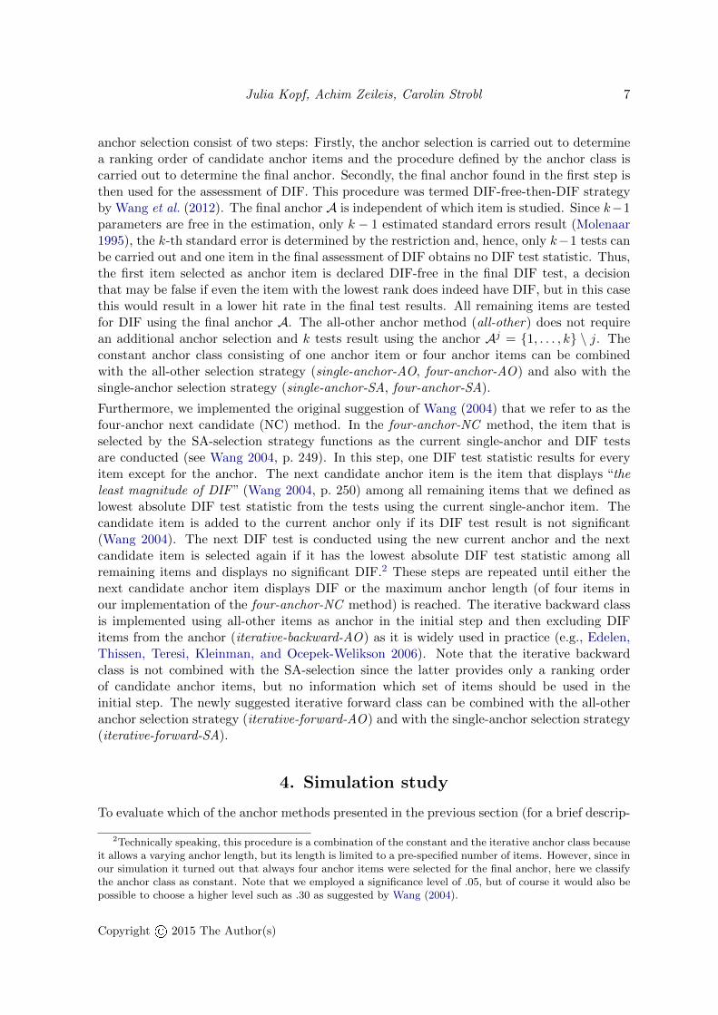
anchor selection consist of two steps: Firstly, the anchor selection is carried out to determinea ranking order of candidate anchor items and the procedure defined by the anchor class iscarried out to determine the final anchor. Secondly, the final anchor found in the first step isthen used for the assessment of DIF. This procedure was termed DIF-free-then-DIF strategyby Wang et al. (2012). The final anchor A is independent of which item is studied. Since k−1parameters are free in the estimation, only k − 1 estimated standard errors result (Molenaar1995), the k-th standard error is determined by the restriction and, hence, only k−1 tests canbe carried out and one item in the final assessment of DIF obtains no DIF test statistic. Thus,the first item selected as anchor item is declared DIF-free in the final DIF test, a decisionthat may be false if even the item with the lowest rank does indeed have DIF, but in this casethis would result in a lower hit rate in the final test results. All remaining items are testedfor DIF using the final anchor A. The all-other anchor method (all-other) does not requirean additional anchor selection and k tests result using the anchor Aj = {1, . . . , k} \ j. Theconstant anchor class consisting of one anchor item or four anchor items can be combinedwith the all-other selection strategy (single-anchor-AO, four-anchor-AO) and also with thesingle-anchor selection strategy (single-anchor-SA, four-anchor-SA).
Furthermore, we implemented the original suggestion of Wang (2004) that we refer to as thefour-anchor next candidate (NC) method. In the four-anchor-NC method, the item that isselected by the SA-selection strategy functions as the current single-anchor and DIF testsare conducted (see Wang 2004, p. 249). In this step, one DIF test statistic results for everyitem except for the anchor. The next candidate anchor item is the item that displays “theleast magnitude of DIF” (Wang 2004, p. 250) among all remaining items that we defined aslowest absolute DIF test statistic from the tests using the current single-anchor item. Thecandidate item is added to the current anchor only if its DIF test result is not significant(Wang 2004). The next DIF test is conducted using the new current anchor and the nextcandidate item is selected again if it has the lowest absolute DIF test statistic among allremaining items and displays no significant DIF.2 These steps are repeated until either thenext candidate anchor item displays DIF or the maximum anchor length (of four items inour implementation of the four-anchor-NC method) is reached. The iterative backward classis implemented using all-other items as anchor in the initial step and then excluding DIFitems from the anchor (iterative-backward-AO) as it is widely used in practice (e.g., Edelen,Thissen, Teresi, Kleinman, and Ocepek-Welikson 2006). Note that the iterative backwardclass is not combined with the SA-selection since the latter provides only a ranking orderof candidate anchor items, but no information which set of items should be used in theinitial step. The newly suggested iterative forward class can be combined with the all-otheranchor selection strategy (iterative-forward-AO) and with the single-anchor selection strategy(iterative-forward-SA).
4. Simulation study
To evaluate which of the anchor methods presented in the previous section (for a brief descrip-
2Technically speaking, this procedure is a combination of the constant and the iterative anchor class becauseit allows a varying anchor length, but its length is limited to a pre-specified number of items. However, since inour simulation it turned out that always four anchor items were selected for the final anchor, here we classifythe anchor class as constant. Note that we employed a significance level of .05, but of course it would also bepossible to choose a higher level such as .30 as suggested by Wang (2004).
Copyright© 2015 The Author(s)
8 Anchor Methods for DIF Detection
Anchorclass
Anchorselection
Combination Initial step and anchor selection strategy
all-other none all-other Initial step: Each item is tested for DIF using allremaining items as anchor.
cf. e.g., Woods(2009)
Selection strategy: No additional selection strategy isrequired.
constant AO single-anchor-AO Initial step: Each item is tested for DIF using allremaining items as anchor.
Woods (2009) Selection strategy: The item with the lowest absoluteDIF statistic (AO) is chosen.
SA single-anchor-SA Initial step: Each item is tested for DIF using every otheritem as single-anchor.
Wang (2004) Selection strategy: The item with the smallest number ofsignificant DIF tests (SA) is chosen.
AO four-anchor-AO Initial step: Each item is tested for DIF using allremaining items as anchor.
Woods (2009);Wang et al. (2012)
Selection strategy: The four anchor items correspondingto the lowest ranks of the absolute DIF statistics fromthe initial step (AO) are chosen.
SA four-anchor-SA Initial step: Each item is tested for DIF using every otheritem as single-anchor.
Wang (2004) Selection strategy: The four anchor items correspondingto the smallest number of significant DIF tests (SA) arechosen.
NC four-anchor-NC Initial step: Each item is tested for DIF using every otheritem as single-anchor.
proposed by Wang(2004)
Selection strategy: The first anchor is found as insingle-anchor-SA; the next candidate anchor item (up tothree) is found from tests using the current anchor if itsresult corresponds to the lowest non-significant absolutetest statistic and is then added to the current anchor.
iterativebackward
AO iterative-backward-AO
Initial step: Each item is tested for DIF using allremaining items as anchor.
e.g., Drasgow(1987)
Selection strategy: Iteratively, all items displaying DIFare excluded from the anchor and the next DIF test withthe current anchor is conducted.
iterativeforward
AO iterative-forward-AO
Initial step: Each item is tested for DIF using allremaining items as anchor.Selection strategy: As long as the current anchor isshorter than the number of currently presumed DIF-freeitems, the next item with the lowest rank in the initialstep (AO) is added to the anchor.
SA iterative-forward-SA
Initial step: Each item is tested for DIF using every otheritem as single-anchor.Selection strategy: As long as the current anchor isshorter than the number of currently presumed DIF-freeitems, the next item with the smallest number ofsignificant test results in the initial step (SA) is added tothe anchor.
Table 1: Classification and nomenclature of the investigated anchor methods.
Copyright© 2015 The Author(s)
Julia Kopf, Achim Zeileis, Carolin Strobl 9
tion and nomenclature see again Table 1) are best suited to correctly classify items with andwithout DIF, an extensive simulation study is conducted. Details about the background andmotivation of our simulation study are provided in the appendix. 2000 data sets (i.e. repli-cations) are generated from each of 77 different simulation settings. For every data set, theitem-wise Wald test (see Section 2) – based on one out of nine investigated anchor methods– is conducted at the significance level of .05 in the free R system for statistical computing(R Core Team 2013). A short description of the study design is given in the following para-graphs. Parts of the simulation design were inspired by the settings used by Wang et al.(2012), Woods (2009) and Wang (2004).
4.1. Data generating process
Each data set corresponds to the simulated responses of two groups of subjects (the reference(ref) and the focal (foc) group) in a test with k = 40 items. We also considered different testlengths of 20, 60, or 80 items (results not shown). In all cases the results were qualitativelysimilar albeit the differences between the iterative forward and constant four anchor class aresomewhat smaller for 20 items (due to more similar anchor lengths) and larger for 60 and 80.
Person and item parameters. In the following simulation study, we have included abilitydifferences, since this case is often found more challenging for the methods than a situationwhere no ability differences are present (see, e.g., Penfield 2001). The person parametersare generated from a normal ability distribution with a higher mean for the reference groupθref ∼ N(0, 1) than for the focal group θfoc ∼ N(−1, 1) similar to Wang et al. (2012). For theitem parameters we chose the values that were already used by Wang et al. (2012).3
DIF items. In case of DIF, the first 15%, 30% or 45% of the items (see Section Directions andproportions of DIF below) are chosen to display uniform DIF by setting the difference in theitem parameters of reference and focal group ∆DIF = βrefj −βfocj to +.6 or −.6 (consistent withthe intended direction of DIF). These differences have been used in previous DIF simulationstudies (Swaminathan and Rogers 1990; Finch 2005; Wang et al. 2012) and reflect a moderateeffect size measured by Raju’s area (Raju 1988; Jodoin and Gierl 2001).
IRT model. The responses in each group follow the Rasch model. They are generated in twosteps: The probability of person i solving item j is computed by inserting the correspondingitem and person parameters in the Rasch model formula 6. The binary responses are thendrawn from a binomial distribution with the resulting probabilities.
P (Uij = 1 | θi, βj) =exp(θi − βj)
1 + exp(θi − βj)(6)
4.2. Manipulated variables
Three main conditions determine the specification of the manipulated variables: One conditionunder the null hypothesis where no DIF is present and two conditions under the alternative
3In addition to these item parameter values β = (−2.522, −1.902, −1.351, −1.092, −0.234, −0.317, 0.037,0.268, −0.571, 0.317, 0.295, 0.778, 1.514, 1.744, 1.951, −1.152, −0.526, 1.104, 0.961, 1.314, −2.198, −1.621,−0.761, −1.179, −0.610, −0.291, 0.067, 0.706, −2.713, 0.213, 0.116, 0.273, 0.840, 0.745, 1.485, −1.208, 0.189,0.345, 0.962, 1.592), we have replicated the main results with various other item parameter settings (resultsnot shown). Therefore we are confident that the different behavior of the anchor methods is not limited to thesettings investigated here.
Copyright© 2015 The Author(s)
10 Anchor Methods for DIF Detection
where DIF is present.
Sample sizes. The sample sizes in reference and focal group are defined by the following pairs(nref, nfoc) ∈ {(250, 250), (500, 250), (500, 500), (750, 500), (750, 750),. . ., (1500, 1500)}. Thus,both equal and different group sizes are considered.
Directions and proportions of DIF. Under the condition of the null hypothesis (no DIF ), onlythe sample sizes are varied. The two remaining conditions represent the alternative hypothesiswhere DIF is present, but they differ with respect to the direction of DIF: The second conditionrepresents balanced DIF. Here, each DIF item favors either the reference or the focal groupbut no systematic advantage for one group remains because the effects cancel out. For thethird unbalanced DIF condition a systematic disadvantage for the focal group is generatedsuch that every DIF item favors the reference group. In addition to the sample size, also theproportion of DIF is manipulated including the following percentages p ∈ {15%, 30%, 45%}.The sample sizes, the DIF percentages and the DIF conditions (balanced and unbalanced)were fully crossed.
4.3. Outcome variables
To allow for a comparison of the anchor methods, the classification accuracy of the DIF testsis evaluated by means of false alarm rate and hit rate.
False alarm rate. For a single replication the false alarm rate is defined as the proportionof DIF-free items that are (erroneously) diagnosed with DIF. The estimated false alarm ratefor each experimental setting is computed as the mean over all 2000 replications and, thus,corresponds to the type I error rate. Similarly, the standard error is estimated as the squareroot of the unbiased sample variance over all replications.
Hit rate. Analogously, for a single replication the hit rate is computed as the proportion ofDIF items that are (correctly) diagnosed with DIF. The hit rate is only defined in conditionsthat include DIF items, namely in the balanced and unbalanced condition. The estimatedhit rate and the standard error are again computed as mean and standard deviation over all2000 replications and correspond to the power of the statistical test and its variation.
Further outcome variables. Moreover, the percentage of replications where at least one item inthe anchor is a simulated DIF item (risk of contamination) is computed over all replicationsof one setting. The average proportion of simulated DIF items as compared to the overallnumber of anchor items (degree of contamination) is computed, too, for replications wherethe anchor is contaminated. Average false alarm rates are also computed separately for thetests based on a contaminated and for the tests based on a pure (not contaminated) anchorto allow for a more detailed interpretation of the results.
5. Results
5.1. Null hypothesis: No DIF
In the first condition, all items were truly DIF-free. Therefore, only the false alarm rates(proportions of DIF-free items that were diagnosed with DIF) were computed and are dis-played in Figure C.1 in the appendix. The standard errors are reported in Table C.1 in theappendix for equal sample sizes.
Copyright© 2015 The Author(s)
Julia Kopf, Achim Zeileis, Carolin Strobl 11
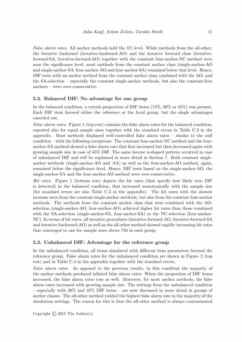
False alarm rates. All anchor methods held the 5% level. While methods from the all-other,the iterative backward (iterative-backward-AO) and the iterative forward class (iterative-forward-SA, iterative-forward-AO) together with the constant four-anchor-NC method werenear the significance level, most methods from the constant anchor class (single-anchor-AOand single-anchor-SA; four-anchor-AO and four-anchor-SA) remained below that level. Hence,DIF tests with an anchor method from the constant anchor class combined with the AO- andthe SA-selection – especially the constant single-anchor methods, but also the constant-fouranchors – were over-conservative.
5.2. Balanced DIF: No advantage for one group
In the balanced condition, a certain proportion of DIF items (15%, 30% or 45%) was present.Each DIF item favored either the reference or the focal group, but the single advantagescanceled out.
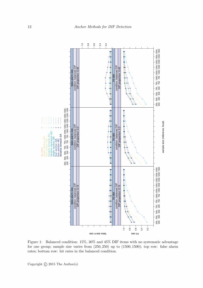
False alarm rates. Figure 1 (top row) contains the false alarm rates for the balanced condition,reported also for equal sample sizes together with the standard errors in Table C.2 in theappendix. Most methods displayed well-controlled false alarm rates – similar to the nullcondition – with the following exceptions: The constant four-anchor-NC method and the four-anchor-SA method showed a false alarm rate that first increased but then decreased again withgrowing sample size in case of 45% DIF. The same inverse u-shaped pattern occurred in caseof unbalanced DIF and will be explained in more detail in Section 7. Both constant single-anchor methods (single-anchor-AO and -SA) as well as the four-anchor-AO method, again,remained below the significance level. Hence, DIF tests based on the single-anchor-AO, thesingle-anchor-SA and the four-anchor-AO method were over-conservative.
Hit rates. Figure 1 (bottom row) depicts the hit rates (that specify how likely true DIFis detected) in the balanced condition, that increased monotonically with the sample size(for standard errors see also Table C.3 in the appendix). The hit rates with the slowestincrease were from the constant single-anchor methods, but also from the constant four-anchormethods. The methods from the constant anchor class that were combined with the AO-selection (single-anchor-AO, four-anchor-AO) achieved higher hit rates than those combinedwith the SA-selection (single-anchor-SA, four-anchor-SA) or the NC-selection (four-anchor-NC). In terms of hit rates, all iterative procedures (iterative-forward-AO, iterative-forward-SAand iterative-backward-AO) as well as the all-other method showed rapidly increasing hit ratesthat converged to one for sample sizes above 750 in each group.
5.3. Unbalanced DIF: Advantage for the reference group
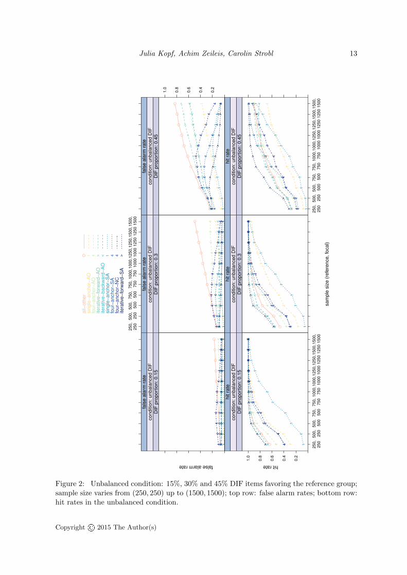
In the unbalanced condition, all items simulated with different item parameters favored thereference group. False alarm rates for the unbalanced condition are shown in Figure 2 (toprow) and in Table C.4 in the appendix together with the standard errors.
False alarm rates. As opposed to the previous results, in this condition the majority ofthe anchor methods produced inflated false alarm rates: When the proportion of DIF itemsincreased, the false alarm rates rose as well. Moreover, for most anchor methods, the falsealarm rates increased with growing sample size. The settings from the unbalanced condition– especially with 30% and 45% DIF items – are now discussed in more detail in groups ofanchor classes. The all-other method yielded the highest false alarm rate in the majority of thesimulation settings. The reason for this is that the all-other method is always contaminated
Copyright© 2015 The Author(s)
12 Anchor Methods for DIF Detection
sa
mp
le s
ize
(re
fere
nce,
foca
l)
hit ratefalse alarm rate
0.2
0.4
0.6
0.8
1.0
25
0,
25
05
00
, 2
50
50
0,
50
07
50
, 5
00
75
0,
75
01
00
0,
75
01
00
0,
10
00
12
50
, 1
00
01
25
0,
12
50
15
00,
12
50
15
00
, 1
500
1
1
1
11
11
11
11
4
4
44
44
44
44
4
>
>
>>
>>
>>
>>
>
<
<
<<
<<
<<
<<
<
1
1
1
1
11
11
11
1
4
4
44
44
44
44
4
4
4
44
44
44
44
4
>
>
>>
>>
>>
>>
>
DIF
pro
po
rtio
n:
0.1
5
co
nd
itio
n:
ba
lan
ce
d D
IF
hit r
ate
1
1
11
11
11
11
1
4
4
44
44
44
44
4
>
>
>>
>>
>>
>>
>
<
<
<<
<<
<<
<<
<
1
1
11
11
11
11
1
4
4
44
44
44
44
4
4
4
44
44
44
44
4
>
>
>>
>>
>>
>>
>
DIF
pro
po
rtio
n:
0.3
co
nd
itio
n:
ba
lan
ce
d D
IF
hit r
ate
25
0,
25
050
0,
250
50
0,
500
750
, 5
00
750
, 7
50
10
00
, 7
50
100
0,
10
00
12
50
, 1
00
012
50
, 1
25
015
00,
125
01
500
, 1
50
0
1
1
11
11
11
11
1
4
4
44
44
44
44
4
>
>
>>
>>
>>
>>
>
<
<
<<
<<
<<
<<
<
1
1
11
11
11
11
1
4
4
44
44
44
44
4
4
4
44
44
44
44
4
>
>
>>
>>
>>
>>
>
DIF
pro
po
rtio
n:
0.4
5
co
nd
itio
n:
ba
lan
ce
d D
IF
hit r
ate
11
11
11
11
11
14
44
44
44
44
44
>>
>>
>>
>>
>>
><
<<
<<
<<
<<
<<
11
11
11
11
11
14
44
44
44
44
44
44
44
44
44
44
4>
>>
>>
>>
>>
>>
DIF
pro
po
rtio
n:
0.1
5
co
nd
itio
n:
ba
lan
ce
d D
IF
fals
e a
larm
ra
te
25
0,
25
05
00
, 2
50
50
0,
50
07
50,
50
07
50
, 7
50
100
0,
75
010
00,
10
00
12
50,
100
01
250
, 1
250
15
00
, 1
250
15
00
, 1
500
11
11
11
11
11
14
44
44
44
44
44
>>
>>
>>
>>
>>
><
<<
<<
<<
<<
<<
11
11
11
11
11
14
44
44
44
44
44
44
44
44
44
44
4>
>>
>>
>>
>>
>>
DIF
pro
po
rtio
n:
0.3
co
nd
itio
n:
ba
lan
ce
d D
IF
fals
e a
larm
ra
te
0.2
0.4
0.6
0.8
1.0
11
11
11
11
11
14
44
44
44
44
44
>>
>>
>>
>>
>>
><
<<
<<
<<
<<
<<
11
11
11
11
11
14
44
44
44
44
44
44
44
44
44
44
4>
>>
>>
>>
>>
>>
DIF
pro
po
rtio
n:
0.4
5
co
nd
itio
n:
ba
lan
ce
d D
IF
fals
e a
larm
ra
te
all−
oth
er
sin
gle
−a
nch
or−
AO
fou
r−a
nch
or−
AO
ite
rative
−fo
rwa
rd−
AO
ite
rative
−b
ackw
ard
−A
Osin
gle
−a
nch
or−
SA
fou
r−a
nch
or−
SA
fou
r−a
nch
or−
NC
ite
rative
−fo
rwa
rd−
SA
1 4 > < 1 4 4 >
Figure 1: Balanced condition: 15%, 30% and 45% DIF items with no systematic advantagefor one group; sample size varies from (250, 250) up to (1500, 1500); top row: false alarmrates; bottom row: hit rates in the balanced condition.
Copyright© 2015 The Author(s)
Julia Kopf, Achim Zeileis, Carolin Strobl 13
sa
mp
le s
ize
(re
fere
nce,
foca
l)
hit ratefalse alarm rate
0.2
0.4
0.6
0.8
1.0
25
0,
25
05
00
, 2
50
50
0,
50
07
50
, 5
00
75
0,
75
01
00
0,
75
01
00
0,
10
00
125
0,
10
00
12
50
, 1
25
01
50
0,
12
50
15
00,
15
00
1
1
1
1
11
11
11
1
4
4
44
44
44
44
4
>
>
>>
>>
>>
>>
>
<
<
<<
<<
<<
<<
<
11
1
1
1
1
11
11
1
4
4
4
4
44
44
44
4
4
4
4
4
44
44
44
4
>
>
>>
>>
>>
>>
>
DIF
pro
po
rtio
n:
0.1
5
co
nd
itio
n:
un
ba
lan
ce
d D
IF
hit r
ate
11
1
1
11
11
11
1
4
4
4
4
44
44
44
4
>
>
>>
>>
>>
>>
>
<
<
<<
<<
<<
<<
<
11
11
1
1
1
1
11
1
4
4
4
4
44
44
44
4
44
4
4
44
44
44
4
>
>
>>
>>
>>
>>
>
DIF
pro
po
rtio
n:
0.3
co
nd
itio
n:
un
ba
lan
ce
d D
IF
hit r
ate
250
,25
05
00
, 2
50
500
, 5
00
75
0,
500
75
0,
750
100
0,
75
010
00
, 1
00
01
25
0,
10
00
125
0,
12
50
15
00,
125
01
500
, 1
50
0
11
11
11
11
11
1
44
44
44
44
44
4
>>
>>
>>
>>
>>
>
<<
<<
<<
<<
<<
<
11
11
11
1
1
11
1
44
44
4
4
44
44
4
44
44
44
44
44
4
>
>
>
>
>>
>>
>>
>
DIF
pro
po
rtio
n:
0.4
5
co
nd
itio
n:
un
ba
lan
ce
d D
IF
hit r
ate
11
11
11
11
11
14
44
44
44
44
44
>>
>>
>>
>>
>>
><
<<
<<
<<
<<
<<
11
11
11
11
11
14
44
44
44
44
44
44
44
44
44
44
4>
>>
>>
>>
>>
>>
DIF
pro
po
rtio
n:
0.1
5
co
nd
itio
n:
un
ba
lan
ce
d D
IF
fals
e a
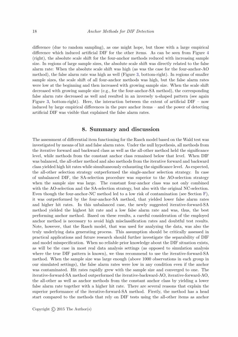
larm
ra
te
25
0,
25
05
00
, 2
50
50
0,
50
07
50
, 5
00
75
0,
75
010
00,
75
01
000
, 1
000
12
50
, 1
000
12
50,
125
015
00,
125
015
00,
150
0
11
11
11
11
11
14
44
44
44
44
44
>>
>>
>>
>>
>>
><
<<
<<
<<
<<
<<
11
11
11
11
11
1
44
44
44
44
44
4
44
44
44
44
44
4>
>>
>>
>>
>>
>>
DIF
pro
po
rtio
n:
0.3
co
nd
itio
n:
un
ba
lan
ce
d D
IF
fals
e a
larm
ra
te
0.2
0.4
0.6
0.8
1.0
11
11
11
11
11
1
44
44
44
44
44
4
>>
>>
>>
>>
>>
>
<<
<<
<<
<<
<<
<
11
11
11
11
11
1
44
44
44
44
44
4
44
44
44
44
44
4>
>>
>>
>>
>>
>>
DIF
pro
po
rtio
n:
0.4
5
co
nd
itio
n:
un
ba
lan
ce
d D
IF
fals
e a
larm
ra
te
all−
oth
er
sin
gle
−a
nch
or−
AO
fou
r−a
nch
or−
AO
ite
rative
−fo
rwa
rd−
AO
ite
rative
−b
ackw
ard
−A
Osin
gle
−a
nch
or−
SA
fou
r−a
nch
or−
SA
fou
r−a
nch
or−
NC
ite
rative
−fo
rwa
rd−
SA
1 4 > < 1 4 4 >
Figure 2: Unbalanced condition: 15%, 30% and 45% DIF items favoring the reference group;sample size varies from (250, 250) up to (1500, 1500); top row: false alarm rates; bottom row:hit rates in the unbalanced condition.
Copyright© 2015 The Author(s)
14 Anchor Methods for DIF Detection
in situations where more than one item has DIF. On average, the mean item parameters ofthe reference group were lower than the mean item parameters of the focal group. Thesemean differences in the item parameters shifted the scales of focal and reference group apartwhen the all-other method defined the restriction (similar to the instructive example in theappendix). These artificial differences became significant when the sample size increased and,thus, resulted in an inflated false alarm rate. For methods from the constant anchor class,the selection strategy explains the false alarm rates: The strategy of selecting anchors basedon the DIF tests with all-other items as anchor yielded biased DIF test results that induceda high false alarm rate when the sample size was large (as illustrated and discussed in moredetail regarding the impact of contamination in Section F). Constant anchors selected by thesingle-anchor strategy produced lower false alarm rates in regions of medium or large samplesizes. Here, again, an inversely u-shaped form is visible. After a certain point, the falsealarm rates decreased again (a detailed explanation will be given in Section 7). The constantsingle-anchor methods showed lower false alarm rates than the corresponding constant four-anchor methods. For all constant methods, the single-anchor-SA method had the lowest falsealarm rate when the sample size was large. The method from the iterative backward anchorclass, which started the initial step by using the all-other method, also led to inflated falsealarm rates that rose when sample size increased. Methods from the iterative forward classdisplayed heterogeneous false alarm rates. The iterative-forward-AO method led to increasedfalse alarm rates – similar to the constant methods with the AO-selection criterion – in thesetting with 30% or 45% DIF. The clearly best iterative method in terms of a low false alarmrate was the new iterative-forward-SA method.
Hit rates. The hit rate in the unbalanced condition (cf. Figure 2, bottom row, and Table C.5in the appendix) in the settings of larger proportions of DIF items was different: Generally,the overall level of the hit rate was lower. Methods from the constant anchor class showedthe slowest increase with the sample size. These methods also had lower hit rates comparedto the methods from the iterative forward or backward class that were the only methodsthat displayed rapidly increasing and high hit rates. The all-other method was between theconstant anchor methods and the iterative anchor methods. The new iterative-forward-SAmethod provided the highest hit rate and a rapid rise of the hit rate with increasing samplesize. In case of 45% DIF, it displayed a much higher hit rate compared to all remainingmethods in the majority of the simulated settings. The SA-selection strategy in combinationwith methods from the constant anchor class was more suitable than the AO-selection strategyregarding the hit rates when the sample size was large. The simplified four-anchor-SA methodoutperformed the originally suggested constant four-anchor method (four-anchor-NC) in termsof higher hit rates (and lower false alarm rates). The iterative forward procedure with theSA-selection was equal or superior to the iterative-forward-AO method over the entire rangeof simulated sample sizes. When accounting for both, the false alarm rate and the hit rate,the newly suggested iterative-forward-SA method is the only reasonable choice among theinvestigated methods in our simulated settings.
6. The impact of anchor contamination
As discussed in Section 2 and in the appendix the contamination of the anchor may induceartificial DIF and, thus, lead to a seriously inflated false alarm rate. New anchor methods areoften judged by their ability to correctly locate a completely DIF-free (i.e. pure, uncontami-
Copyright© 2015 The Author(s)
Julia Kopf, Achim Zeileis, Carolin Strobl 15
sample size (reference, focal)
0.0
0.2
0.4
0.6
0.8
1.0
250,250
500, 250
500, 500
750, 500
750, 750
1000, 750
1000, 1000
1250, 1000
1250, 1250
1500, 1250
1500, 1500
1 11
1
11
1
1
11
1
44
44
44
44
4 44
>>
>>
>>
>>
> >>
<<
< < << <
<< <
<
1 11
1
11
11
1 11
44
44 4 4
4 44 4 44
4
4
4
44
44
4 4 4
> > > >>
>> > > > >
DIF proportion: 0.45
condition: unbalanced DIF
false alarm rate (contaminated anchor)
1 11 1
1 1 1 1 1 1 14 4
4 4 4 4 4 4 4 4 4<
<< < <
1 11 1 1 1 1 1
1 1 1
4 44 4
4 44 4
4 4 4
4 44 4 4 4 4 4
4 4 4>
> > > > > > >
DIF proportion: 0.45
condition: unbalanced DIF
false alarm rate (pure anchor)
1 11
1 1 1 1 1 1 1 1
4 44 4 4 4 4 4 4 4 4
> > > > > > > > > > >< < < < < < < < < <<
11
1 1
1 1
11
11
1
4 44 4
44
4
4
44
4
4 4
4 4
44
4
4
44
4
> > > > > >
>
>
>>
>
DIF proportion: 0.45
condition: unbalanced DIF
risk of contamination
250,250
500, 250
500, 500
750, 500
750, 750
1000, 750
1000, 1000
1250, 1000
1250, 1250
1500, 1250
1500, 1500
0.0
0.2
0.4
0.6
0.8
1.01 1 1 1 1 1 1 1 1 1 1
4 44 4 4 4 4 4 4 4 4
> > > > > > > > > > >< <
< << < < < < <
<
1 1 1 1 1 1 1 1 1 1 1
4 44 4
4 44 4 4 4 4
44
4 44
4 4 4 4 4 4
> >>
>
>>
> > > > >
DIF proportion: 0.45
condition: unbalanced DIF
degree of contamination
all−othersingle−anchor−AOfour−anchor−AOiterative−forward−AOiterative−backward−AOsingle−anchor−SAfour−anchor−SAfour−anchor−NCiterative−forward−SA
1
4
><
1
4
4
>
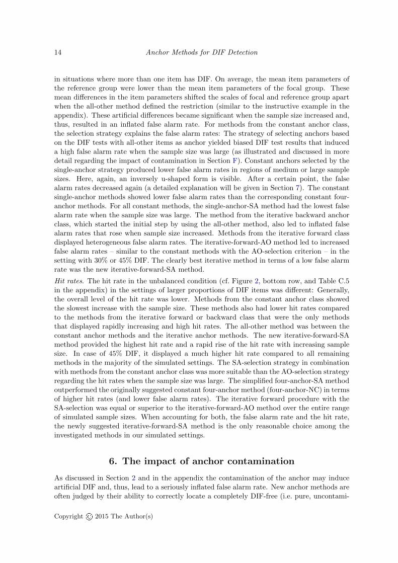
Figure 3: Condition of unbalanced DIF with 45% DIF items favoring the reference group;sample size ranges from (250, 250) to (1500, 1500); top-left: risk of contaminated anchors (atleast one DIF item included in the anchor); top-right: degree of contamination (proportionof DIF items in contaminated anchors); bottom-left: false alarm rates when the anchor iscontaminated; bottom-right: false alarm rates when the anchor is pure (not contaminated).
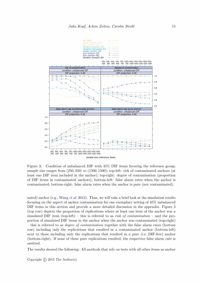
nated) anchor (e.g., Wang et al. 2012). Thus, we will take a brief look at the simulation resultsfocusing on the aspect of anchor contamination for one exemplary setting of 45% unbalancedDIF items in this section and provide a more detailed discussion in the appendix. Figure 3(top row) depicts the proportion of replications where at least one item of the anchor was asimulated DIF item (top-left) – this is referred to as risk of contamination – and the pro-portion of simulated DIF items in the anchor when the anchor was contaminated (top-right)– this is referred to as degree of contamination together with the false alarm rates (bottomrow) including only the replications that resulted in a contaminated anchor (bottom-left)next to those including only the replications that resulted in a pure (i.e. DIF-free) anchor(bottom-right). If none of these pure replications resulted, the respective false alarm rate isomitted.
The results showed the following: All methods that rely on tests with all other items as anchor
Copyright© 2015 The Author(s)
16 Anchor Methods for DIF Detection
(namely the all-other, single-anchor-AO, four-anchor-AO, iterative-forward-AO, iterative-backward-AO) displayed risks and also degrees of contamination that did not or only slightly decreasewith the sample size. The overall risk and degree level depended on the anchor length. Shortanchors, for example, displayed a lower risk of contamination compared to longer anchors.The corresponding false alarm rates with a contaminated anchor increased, since – with in-creasing sample size – the power of detecting artificial DIF (DIF-free items that displayed DIFdue to the chosen anchor method) increased. Those methods that are built using the SA-selection (namely the single-anchor-SA, four-anchor-SA, iterative-forward-SA) showed risksand degrees that decreased with the sample size (except for the degree of the single-anchor).Their false alarm rates in contaminated replications were also lower when the sample size washigh. An interesting finding here is the result for the four-anchor-NC method: It displayeda rapidly decreasing risk of contamination, but also a very high degree of contamination.As a consequence, the false alarm rate in contaminated replications was very high and evenincreased in the sample size. This explains the weak overall performance (see again Figure 2,top row right). This result makes clear that it is not the risk of contamination alone thatdetermines the performance of the anchor method. The iterative-forward-SA method (thatperformed best – in terms of a low false alarm rate together with a high hit rate – in thiscondition, see again Figure 2, right) displayed a higher risk of contamination but a lowerdegree of contamination compared to the four-anchor-NC method. The false alarm rate ofthe iterative-forward-SA method was low, independent of whether the anchor was contami-nated or not (see Figure 3, bottom row). Thus, we conclude that research on anchor methodsshould not only concentrate on the risk of contamination, but also focus on the consequences,which strongly depend on the degree of contamination, i.e. the proportion of DIF-items in thecontaminated anchor. The second astounding finding, which we address in the next section,was that we observed false alarm rates exceeding the significance level, even in the case whenonly pure replications without anchor contamination were regarded (see Figure 3, bottom rowright).
7. Characteristics of the anchor items inducing artificial DIF
In our simulation study, several anchor methods displayed inversely u-shaped false alarmrates that are yet to be explained. There are two mechanisms at work here: On one hand, therisk and the degree of contamination decrease with increasing sample size when the anchorselection strategy works appropriately and, thus, the extent of artificial DIF decreases. Onthe other hand, the power of detecting artificial DIF increases with growing sample size. Onepossible explanation for the inversely u-shaped pattern is the interaction between the de-creasing extent of artificial DIF induced by anchor contamination and the increasing power ofdetecting statistically significant artificial DIF. In the beginning the false alarm rate increasesdue to the increasing power for detecting artificial DIF but at some point the false alarmrate decreases again as the risk of contamination decreases. This explanation is consistentwith the findings from Section F, when the anchor was contaminated and we provide a moredetailed discussion of the contaminated replications in the appendix. However, with this ar-gument we cannot yet explain why the false alarm rates showed a similar pattern for pure(uncontaminated) replications (see again Figure 3, bottom-right), where the single-anchor-SA, the four-anchor-SA as well as the four-anchor-NC method displayed inversely u-shapedfalse alarm rates. Therefore, the presence of artificial DIF induced by contamination alone
Copyright© 2015 The Author(s)
Julia Kopf, Achim Zeileis, Carolin Strobl 17
sample size (reference, focal)
−1.5
−1.0
−0.5
0.0
250,250
500, 250
500, 500
750, 500
750, 750
1000, 750
1000, 1000
1250, 1000
1250, 1250
1500, 1250
1500, 1500
4 4 4 4 4 4 4 4 4 4 4
4 44 4
44
44
4 44
4 4 4 4 4 4 4 4 4 4 4
DIF proportion: 0.45
condition: unbalanced DIF
scale shift (contaminated anchor)
250,250
500, 250
500, 500
750, 500
750, 750
1000, 750
1000, 1000
1250, 1000
1250, 1250
1500, 1250
1500, 1500
44
4 44
44 4
4 4 4
4 4 4 4
44
44
4 44
4 4 4 44
44
4
44
4
4 4 4 4 4 4 4 4 4 4 4
DIF proportion: 0.45
condition: unbalanced DIF
scale shift (pure anchor)
four−anchor−AOfour−anchor−SAfour−anchor−NCbenchmark
4
4
4
4
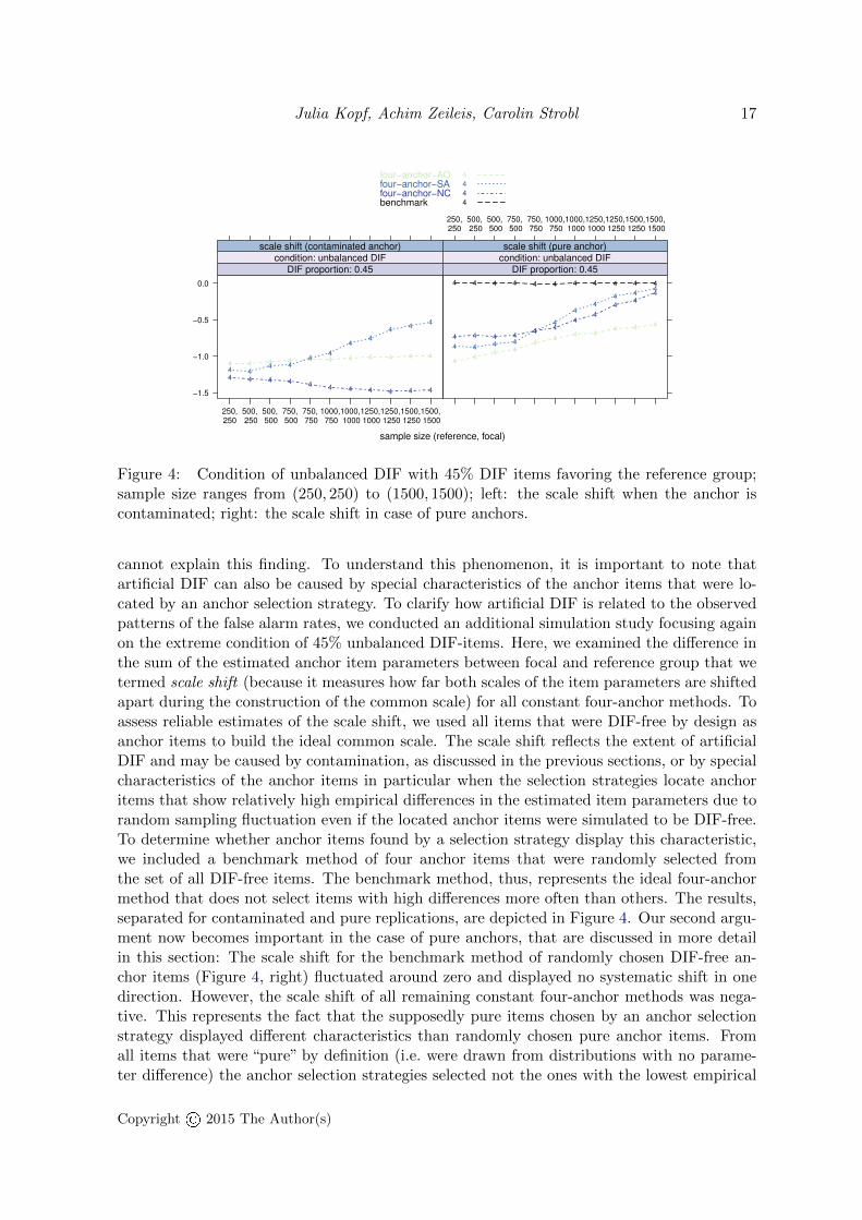
Figure 4: Condition of unbalanced DIF with 45% DIF items favoring the reference group;sample size ranges from (250, 250) to (1500, 1500); left: the scale shift when the anchor iscontaminated; right: the scale shift in case of pure anchors.
cannot explain this finding. To understand this phenomenon, it is important to note thatartificial DIF can also be caused by special characteristics of the anchor items that were lo-cated by an anchor selection strategy. To clarify how artificial DIF is related to the observedpatterns of the false alarm rates, we conducted an additional simulation study focusing againon the extreme condition of 45% unbalanced DIF-items. Here, we examined the difference inthe sum of the estimated anchor item parameters between focal and reference group that wetermed scale shift (because it measures how far both scales of the item parameters are shiftedapart during the construction of the common scale) for all constant four-anchor methods. Toassess reliable estimates of the scale shift, we used all items that were DIF-free by design asanchor items to build the ideal common scale. The scale shift reflects the extent of artificialDIF and may be caused by contamination, as discussed in the previous sections, or by specialcharacteristics of the anchor items in particular when the selection strategies locate anchoritems that show relatively high empirical differences in the estimated item parameters due torandom sampling fluctuation even if the located anchor items were simulated to be DIF-free.To determine whether anchor items found by a selection strategy display this characteristic,we included a benchmark method of four anchor items that were randomly selected fromthe set of all DIF-free items. The benchmark method, thus, represents the ideal four-anchormethod that does not select items with high differences more often than others. The results,separated for contaminated and pure replications, are depicted in Figure 4. Our second argu-ment now becomes important in the case of pure anchors, that are discussed in more detailin this section: The scale shift for the benchmark method of randomly chosen DIF-free an-chor items (Figure 4, right) fluctuated around zero and displayed no systematic shift in onedirection. However, the scale shift of all remaining constant four-anchor methods was nega-tive. This represents the fact that the supposedly pure items chosen by an anchor selectionstrategy displayed different characteristics than randomly chosen pure anchor items. Fromall items that were “pure” by definition (i.e. were drawn from distributions with no parame-ter difference) the anchor selection strategies selected not the ones with the lowest empirical
Copyright© 2015 The Author(s)
18 Anchor Methods for DIF Detection
difference (due to random sampling), as one might hope, but those with a large empiricaldifference which induced artificial DIF for the other items. As can be seen from Figure 4(right), the absolute scale shift for the four-anchor methods reduced with increasing samplesize. In regions of large sample sizes, the absolute scale shift was directly related to the falsealarm rate: When the absolute scale shift was high (as was the case for the four-anchor-AOmethod), the false alarm rate was high as well (Figure 3, bottom-right). In regions of smallersample sizes, the scale shift of all four-anchor methods was high, but the false alarm rateswere low at the beginning and then increased with growing sample size. When the scale shiftdecreased with growing sample size (e.g., for the four-anchor-SA method), the correspondingfalse alarm rate decreased as well and resulted in an inversely u-shaped pattern (see againFigure 3, bottom-right). Here, the interaction between the extent of artificial DIF – nowinduced by large empirical differences in the pure anchor items – and the power of detectingartificial DIF was visible that explained the false alarm rates.
8. Summary and discussion
The assessment of differential item functioning for the Rasch model based on the Wald test wasinvestigated by means of hit and false alarm rates. Under the null hypothesis, all methods fromthe iterative forward and backward class as well as the all-other method held the significancelevel, while methods from the constant anchor class remained below that level. When DIFwas balanced, the all-other method and also methods from the iterative forward and backwardclass yielded high hit rates while simultaneously exhausting the significance level. As expected,the all-other selection strategy outperformed the single-anchor selection strategy. In caseof unbalanced DIF, the SA-selection procedure was superior to the AO-selection strategywhen the sample size was large. The constant four-anchor class was not only combinedwith the AO-selection and the SA-selection strategy, but also with the original NC-selection.Even though the four-anchor-NC method led to a low risk of contamination (see Section F),it was outperformed by the four-anchor-SA method, that yielded lower false alarm ratesand higher hit rates. In this unbalanced case, the newly suggested iterative-forward-SAmethod yielded the highest hit rate and a low false alarm rate and was, thus, the bestperforming anchor method. Based on these results, a careful consideration of the employedanchor method is necessary to avoid high misclassification rates and doubtful test results.Note, however, that the Rasch model, that was used for analyzing the data, was also thetruly underlying data generating process. This assumption should be critically assessed inpractical applications and future research should further investigate the separability of DIFand model misspecification. When no reliable prior knowledge about the DIF situation exists,as will be the case in most real data analysis settings (as opposed to simulation analysiswhere the true DIF pattern is known), we thus recommend to use the iterative-forward-SAmethod. When the sample size was large enough (above 1000 observations in each group inour simulated settings), the false alarm rates were low in any condition even if the anchorwas contaminated. Hit rates rapidly grew with the sample size and converged to one. Theiterative-forward-SA method outperformed the iterative-backward-AO, iterative-forward-AO,the all-other as well as anchor methods from the constant anchor class by yielding a lowerfalse alarm rate together with a higher hit rate. There are several reasons that explain thesuperior performance of the iterative-forward-SA method. Firstly, the method has a headstart compared to the methods that rely on DIF tests using the all-other items as anchor
Copyright© 2015 The Author(s)
Julia Kopf, Achim Zeileis, Carolin Strobl 19
(e.g., the classical iterative procedures, such as the iterative-backward-AO). While the latterstart with a criterion that is severely biased when DIF is unbalanced, the iterative-forward-SA method does not require that DIF effects almost cancel out (for a discussion see Wang2004). Secondly, the SA-selection strategy combined with the iterative forward anchor classalso performed well in case of balanced DIF. While the AO-selection strategy performedbetter than the SA-selection strategy when it was combined with the methods from theconstant anchor class, the advantage in combination with the iterative forward class appearednegligible. Thirdly, our study showed that the consequences of contamination depend on theproportion of contaminated items rather than on the risk of contamination itself. Therefore,the iterative-forward-SA method yielded better results in DIF analysis even though the anchorwas long and, thus, often contaminated. The risk of contamination decreased with increasingsample size and, beyond that, the proportion of DIF items in the contaminated anchor (thedegree of contamination) decreased. Fourthly, the iterative forward anchor class adds itemsto the anchor as long as the number of anchor items is smaller than the set of presumedDIF-free items. If the sample size is large enough, this leads to the desirable property, thatit produces a longer anchor when the proportion of DIF items is low and a shorter anchorif the proportion of DIF items is high, similar to the iterative backward method.4 Anotherastounding finding of our simulations was that anchor items located by an anchor selectionstrategy displayed different characteristics compared to randomly chosen DIF-free items andmay be exactly those items that again induce artificial DIF. Including more anchor items(than, e.g., four anchor items) reduces the artificial scale shift that is induced by anchor itemswith empirical group differences and, thus, can also occur when the anchor is (by definition)pure. The reason for this is that a longer anchor, that contains some items that induceartificial DIF but also several items that do not, shifts the scales of the item parametersless strongly than a shorter anchor, where the proportion of items inducing artificial DIF ishigher. The simulation study presented here was limited to DIF analysis in the Rasch modelusing the Wald test. Thus, future research (the interested reader is referred to the appendix)may investigate the usefulness of the iterative-forward-SA method for other IRT models andcombine it with other DIF detection methods.
Acknowledgments
Julia Kopf is supported by the German Federal Ministry of Education and Research (BMBF)within the project “Heterogeneity in IRT-Models” (grant ID 01JG1060). The authors wouldlike to thank Thomas Augustin for his expert advice and three anonymous reviewers for theirvery helpful and constructive feedback.
References
4It may appear as a drawback that the iterative forward anchor class uses a short anchor in the initialsteps, beginning with only one anchor item located by the respective anchor selection strategy. The resultingDIF tests may lack statistical power due to fact that the anchor is short. However, this does not affect theperformance of the new iterative forward anchor methods since the test results are only used for the decisionwhether the anchor should include one more anchor item. Thus, a small statistical power of the DIF tests inthe first iterations automatically leads to a longer anchor that is expected to increase the power of the actualDIF test in the final step.
Copyright© 2015 The Author(s)
20 Anchor Methods for DIF Detection
Andrich D, Hagquist C (2012). “Real and Artificial Differential Item Functioning.” Journalof Educational and Behavioral Statistics, 37(3), 387–416.
Candell GL, Drasgow F (1988). “An Iterative Procedure for Linking Metrics and AssessingItem Bias in Item Response Theory.” Applied Psychological Measurement, 12(3), 253–260.
Clauser B, Mazor K, Hambleton RK (1993). “The Effects of Purification of Matching Criterionon the Identification of DIF Using the Mantel-Haenszel Procedure.” Applied Measurementin Education, 6(4), 269–279.
Cohen AS, Kim SH, Wollack JA (1996). “An Investigation of the Likelihood Ratio Test forDetection of Differential Item Functioning.” Applied Psychological Measurement, 20(1),15–26.
Drasgow F (1987). “Study of the Measurement Bias of Two Standardized Psychological Tests.”Journal of Applied Psychology, 72(1), 19–29.
Edelen MO, Thissen D, Teresi JA, Kleinman M, Ocepek-Welikson K (2006). “Identification ofDifferential Item Functioning Using Item Response Theory and the Likelihood-based ModelComparison Approach. Application to the Mini-Mental State Examination.” Medical Care,44(22), 134–142.
Eggen T, Verhelst N (2006). “Loss of Information in Estimating Item Parameters in Incom-plete Designs.” Psychometrika, 71(2), 303–322.
Finch H (2005). “The MIMIC Model As a Method for Detecting DIF: Comparison withMantel-Haenszel, SIBTEST, and the IRT Likelihood Ratio.” Applied Psychological Mea-surement, 29(4), 278–295.
Fischer GH (1995). “Derivations of the Rasch Model.” In GH Fischer, IW Molenaar (eds.),Rasch Models – Foundations, Recent Developments, and Applications, chapter 2. Springer,New York.
Frederickx S, Tuerlinckx F, De Boeck P, Magis D (2010). “RIM: A Random Item MixtureModel to Detect Differential Item Functioning.” Journal of Educational Measurement,47(4), 432–457.
Glas CAW, Verhelst ND (1995). “Testing the Rasch Model.” In GH Fischer, IW Molenaar(eds.), Rasch Models – Foundations, Recent Developments, and Applications, chapter 5.Springer, New York.
Gonzalez-Betanzos F, Abad FJ (2012). “The Effects of Purification and the Evaluation ofDifferential Item Functioning with the Likelihood Ratio Test.” Methodology: EuropeanJournal of Research Methods for the Behavioral and Social Sciences, 8(4), 134–145.
Hidalgo-Montesinos MD, Lopez-Pina JA (2002). “Two-Stage Equating in Differential ItemFunctioning Detection under the Graded Response Model with the Raju Area Measuresand the Lord Statistic.” Educational and Psychological Measurement, 62(1), 32–44.
Jodoin MG, Gierl MJ (2001). “Evaluating Type I Error and Power Rates Using an Effect SizeMeasure with the Logistic Regression Procedure for DIF Detection.” Applied Measurementin Education, 14(4), 329–349.
Copyright© 2015 The Author(s)
Julia Kopf, Achim Zeileis, Carolin Strobl 21
Lopez Rivas GE, Stark S, Chernyshenko OS (2009). “The Effects of Referent Item Parameterson Differential Item Functioning Detection Using the Free Baseline Likelihood Ratio Test.”Applied Psychological Measurement, 33(4), 251–265.
Lord F (1980). Applications of Item Response Theory to Practical Testing Problems. LawrenceErlbaum, Hillsdale, New Jersey.
Magis D, Raıche G, Beland S, Gerard P (2011). “A Generalized Logistic Regression Procedureto Detect Differential Item Functioning Among Multiple Groups.” International Journalof Testing, 11(4), 365–386.
McLaughlin ME, Drasgow F (1987). “Lord’s Chi-Square Test of Item Bias With Estimatedand With Known Person Parameters.” Applied Psychological Measurement, 11(2), 161–173.
Mellenbergh GJ (1982). “Contingency Table Models for Assessing Item Bias.” Journal ofEducational Statistics, 7(2), 105–118.
Miller MD, Oshima T (1992). “Effect of Sample Size, Number of Biased Items, and Magnitudeof Bias on a Two-Stage Item Bias Estimation Method.” Applied Psychological Measurement,16(4), 381–388.
Millsap RE, Everson HT (1993). “Methodology Review: Statistical Approaches for AssessingMeasurement Bias.” Applied Psychological Measurement, 17(4), 297–334.
Molenaar IW (1995). “Estimation of Item Parameters.” In GH Fischer, IW Molenaar (eds.),Rasch Models – Foundations, Recent Developments, and Applications, chapter 3. Springer,New York.
Navas-Ara MJ, Gomez-Benito J (2002). “Effects of Ability Scale Purification on the Identifi-cation of DIF.” European Journal of Psychological Assessment, 18(1), 9–15.
Paek I, Han KT (2013). “IRTPRO 2.1 for Windows (Item Response Theory for Patient-Reported Outcomes).” Applied Psychological Measurement, 37(3), 242–252.
Penfield RD (2001). “Assessing Differential Item Functioning Among Multiple Groups: AComparison of Three Mantel-Haenszel Procedures.” Applied Measurement in Education,14(3), 235 – 259.
R Core Team (2013). R: A Language and Environment for Statistical Computing. R Foun-dation for Statistical Computing, Vienna, Austria. URL http://www.R-project.org/.
Raju N (1988). “The Area Between Two Item Characteristic Curves.” Psychometrika, 53(4),495–502.
Shih CL, Wang WC (2009). “Differential Item Functioning Detection Using the MultipleIndicators, Multiple Causes Method with a Pure Short Anchor.” Applied PsychologicalMeasurement, 33(3), 184–199.
Stark S, Chernyshenko OS, Drasgow F (2006). “Detecting Differential Item Functioning withConfirmatory Factor Analysis and Item Response Theory: Toward a Unified Strategy.”Journal of Applied Psychology, 91(6), 1292–1306.
Copyright© 2015 The Author(s)
22 Anchor Methods for DIF Detection
Strobl C, Kopf J, Zeileis A (2010). “Wissen Frauen weniger oder nur das Falsche? Einstatistisches Modell fur unterschiedliche Aufgaben-Schwierigkeiten in Teilstichproben.” InS Trepte, M Verbeet (eds.), Wissenswelten des 21. Jahrhunderts – Erkenntnisse aus demStudentenpisa-Test des SPIEGEL. VS Verlag, Wiesbaden.
Swaminathan H, Rogers HJ (1990). “Detecting Differential Item Functioning Using LogisticRegression Procedures.” Journal of Educational Measurement, 27(4), 361–370.
Thissen D (2001). IRTLRDIF v.2.0b: Software for the Computation of the Statistics In-volved in Item Response Theory Likelihood-Ratio Tests for Differential Item Functioning.Unpublished manuscript, University of North Carolina, Chapel Hill.
Thissen D, Steinberg L, Wainer H (1988). “Use of Item Response Theory in the Study ofGroup Differences in Trace Lines.” In H Wainer, HI Braun (eds.), Test Validity, chapter 10.Lawrence Erlbaum, Hillsdale, New Jersey.
Trepte S, Verbeet M (eds.) (2010). Allgemeinbildung in Deutschland – Erkenntnisse aus demSPIEGEL Studentenpisa-Test. VS Verlag, Wiesbaden.
Wang WC (2004). “Effects of Anchor Item Methods on the Detection of Differential ItemFunctioning within the Family of Rasch Models.” Journal of Experimental Education,72(3), 221–261.
Wang WC, Shih CL, Sun GW (2012). “The DIF-Free-Then-DIF Strategy for the Assessmentof Differential Item Functioning.” Educational and Psychological Measurement, 72(4), 687–708.
Wang WC, Su YH (2004). “Effects of Average Signed Area Between Two Item CharacteristicCurves and Test Purification Procedures on the DIF Detection via the Mantel-HaenszelMethod.” Applied Measurement in Education, 17(2), 113–144.
Wang WC, Yeh YL (2003). “Effects of Anchor Item Methods on Differential Item FunctioningDetection with the Likelihood Ratio Test.” Applied Psychological Measurement, 27(6), 479–498.
Woods CM (2009). “Empirical Selection of Anchors for Tests of Differential Item Functioning.”Applied Psychological Measurement, 33(1), 42–57.
Woods CM, Cai L, Wang M (2013). “The Langer-Improved Wald Test for DIF TestingWith Multiple Groups: Evaluation and Comparison to Two-Group IRT.” Educational andPsychological Measurement, 73(3), 532–547.
Copyright© 2015 The Author(s)
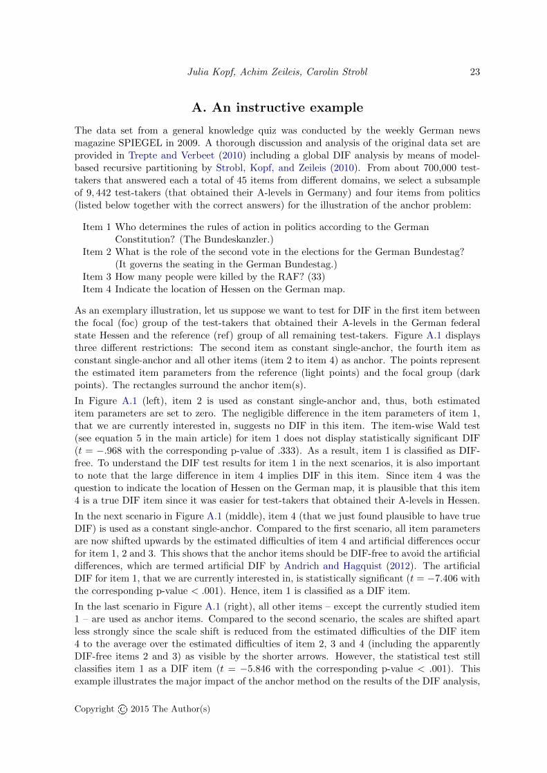
Julia Kopf, Achim Zeileis, Carolin Strobl 23
A. An instructive example
The data set from a general knowledge quiz was conducted by the weekly German newsmagazine SPIEGEL in 2009. A thorough discussion and analysis of the original data set areprovided in Trepte and Verbeet (2010) including a global DIF analysis by means of model-based recursive partitioning by Strobl, Kopf, and Zeileis (2010). From about 700,000 test-takers that answered each a total of 45 items from different domains, we select a subsampleof 9, 442 test-takers (that obtained their A-levels in Germany) and four items from politics(listed below together with the correct answers) for the illustration of the anchor problem:
Item 1 Who determines the rules of action in politics according to the GermanConstitution? (The Bundeskanzler.)
Item 2 What is the role of the second vote in the elections for the German Bundestag?(It governs the seating in the German Bundestag.)
Item 3 How many people were killed by the RAF? (33)Item 4 Indicate the location of Hessen on the German map.
As an exemplary illustration, let us suppose we want to test for DIF in the first item betweenthe focal (foc) group of the test-takers that obtained their A-levels in the German federalstate Hessen and the reference (ref) group of all remaining test-takers. Figure A.1 displaysthree different restrictions: The second item as constant single-anchor, the fourth item asconstant single-anchor and all other items (item 2 to item 4) as anchor. The points representthe estimated item parameters from the reference (light points) and the focal group (darkpoints). The rectangles surround the anchor item(s).
In Figure A.1 (left), item 2 is used as constant single-anchor and, thus, both estimateditem parameters are set to zero. The negligible difference in the item parameters of item 1,that we are currently interested in, suggests no DIF in this item. The item-wise Wald test(see equation 5 in the main article) for item 1 does not display statistically significant DIF(t = −.968 with the corresponding p-value of .333). As a result, item 1 is classified as DIF-free. To understand the DIF test results for item 1 in the next scenarios, it is also importantto note that the large difference in item 4 implies DIF in this item. Since item 4 was thequestion to indicate the location of Hessen on the German map, it is plausible that this item4 is a true DIF item since it was easier for test-takers that obtained their A-levels in Hessen.
In the next scenario in Figure A.1 (middle), item 4 (that we just found plausible to have trueDIF) is used as a constant single-anchor. Compared to the first scenario, all item parametersare now shifted upwards by the estimated difficulties of item 4 and artificial differences occurfor item 1, 2 and 3. This shows that the anchor items should be DIF-free to avoid the artificialdifferences, which are termed artificial DIF by Andrich and Hagquist (2012). The artificialDIF for item 1, that we are currently interested in, is statistically significant (t = −7.406 withthe corresponding p-value < .001). Hence, item 1 is classified as a DIF item.
In the last scenario in Figure A.1 (right), all other items – except the currently studied item1 – are used as anchor items. Compared to the second scenario, the scales are shifted apartless strongly since the scale shift is reduced from the estimated difficulties of the DIF item4 to the average over the estimated difficulties of item 2, 3 and 4 (including the apparentlyDIF-free items 2 and 3) as visible by the shorter arrows. However, the statistical test stillclassifies item 1 as a DIF item (t = −5.846 with the corresponding p-value < .001). Thisexample illustrates the major impact of the anchor method on the results of the DIF analysis,
Copyright© 2015 The Author(s)
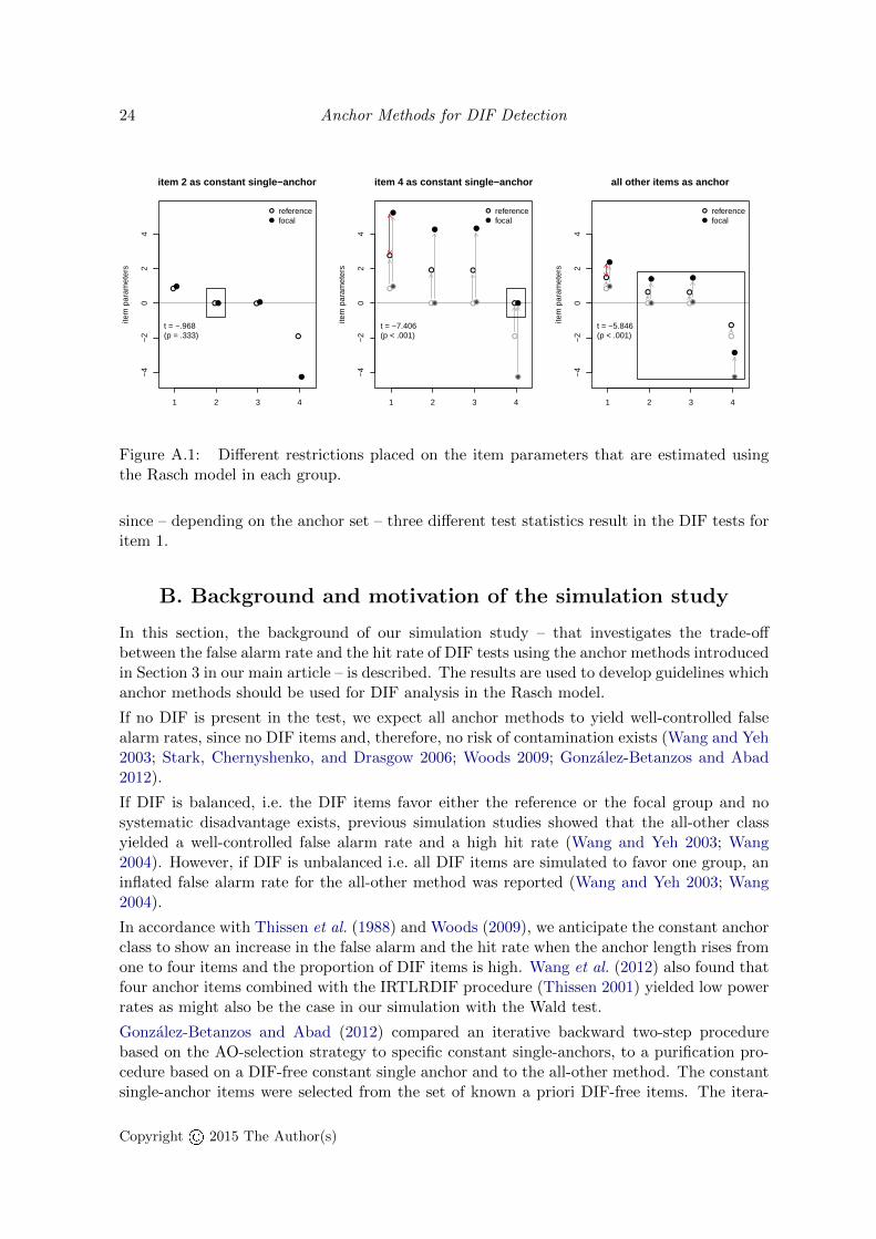
24 Anchor Methods for DIF Detection
item 2 as constant single−anchor
item
par
amet
ers
●
● ●
●
●
● ●
●
1 2 3 4
−4
−2
02
4
●
●
referencefocal
t = −.968(p = .333)
item 4 as constant single−anchor
item
par
amet
ers
●
● ●
●
●
● ●
●
●
● ●
●
●
● ●
●
1 2 3 4
−4
−2
02
4
●
●
referencefocal
t = −7.406(p < .001)
all other items as anchor
item
par
amet
ers
●
● ●
●
●
● ●
●
●
● ●
●
●
● ●
●
1 2 3 4
−4
−2
02
4
●
●
referencefocal
t = −5.846(p < .001)
Figure A.1: Different restrictions placed on the item parameters that are estimated usingthe Rasch model in each group.
since – depending on the anchor set – three different test statistics result in the DIF tests foritem 1.
B. Background and motivation of the simulation study
In this section, the background of our simulation study – that investigates the trade-offbetween the false alarm rate and the hit rate of DIF tests using the anchor methods introducedin Section 3 in our main article – is described. The results are used to develop guidelines whichanchor methods should be used for DIF analysis in the Rasch model.
If no DIF is present in the test, we expect all anchor methods to yield well-controlled falsealarm rates, since no DIF items and, therefore, no risk of contamination exists (Wang and Yeh2003; Stark, Chernyshenko, and Drasgow 2006; Woods 2009; Gonzalez-Betanzos and Abad2012).
If DIF is balanced, i.e. the DIF items favor either the reference or the focal group and nosystematic disadvantage exists, previous simulation studies showed that the all-other classyielded a well-controlled false alarm rate and a high hit rate (Wang and Yeh 2003; Wang2004). However, if DIF is unbalanced i.e. all DIF items are simulated to favor one group, aninflated false alarm rate for the all-other method was reported (Wang and Yeh 2003; Wang2004).
In accordance with Thissen et al. (1988) and Woods (2009), we anticipate the constant anchorclass to show an increase in the false alarm and the hit rate when the anchor length rises fromone to four items and the proportion of DIF items is high. Wang et al. (2012) also found thatfour anchor items combined with the IRTLRDIF procedure (Thissen 2001) yielded low powerrates as might also be the case in our simulation with the Wald test.
Gonzalez-Betanzos and Abad (2012) compared an iterative backward two-step procedurebased on the AO-selection strategy to specific constant single-anchors, to a purification pro-cedure based on a DIF-free constant single anchor and to the all-other method. The constantsingle-anchor items were selected from the set of known a priori DIF-free items. The itera-
Copyright© 2015 The Author(s)
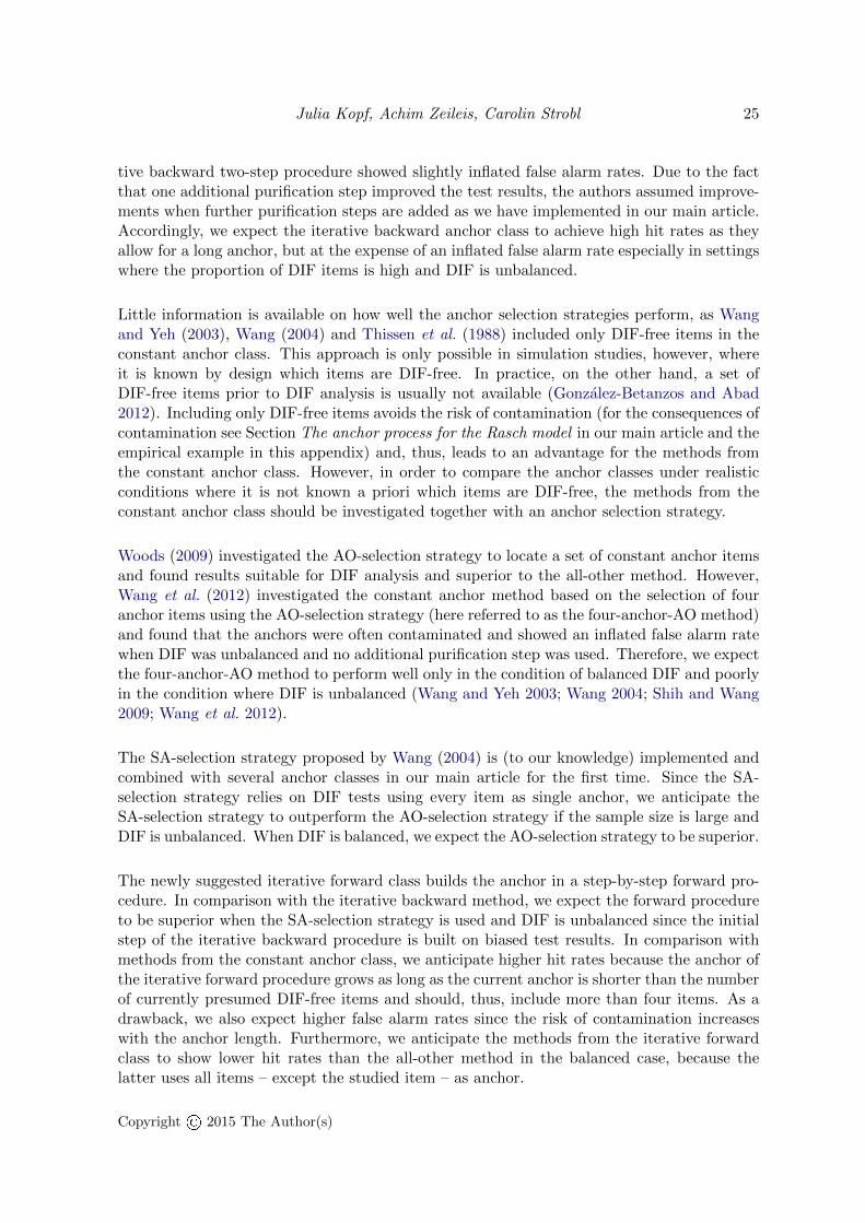
Julia Kopf, Achim Zeileis, Carolin Strobl 25
tive backward two-step procedure showed slightly inflated false alarm rates. Due to the factthat one additional purification step improved the test results, the authors assumed improve-ments when further purification steps are added as we have implemented in our main article.Accordingly, we expect the iterative backward anchor class to achieve high hit rates as theyallow for a long anchor, but at the expense of an inflated false alarm rate especially in settingswhere the proportion of DIF items is high and DIF is unbalanced.
Little information is available on how well the anchor selection strategies perform, as Wangand Yeh (2003), Wang (2004) and Thissen et al. (1988) included only DIF-free items in theconstant anchor class. This approach is only possible in simulation studies, however, whereit is known by design which items are DIF-free. In practice, on the other hand, a set ofDIF-free items prior to DIF analysis is usually not available (Gonzalez-Betanzos and Abad2012). Including only DIF-free items avoids the risk of contamination (for the consequences ofcontamination see Section The anchor process for the Rasch model in our main article and theempirical example in this appendix) and, thus, leads to an advantage for the methods fromthe constant anchor class. However, in order to compare the anchor classes under realisticconditions where it is not known a priori which items are DIF-free, the methods from theconstant anchor class should be investigated together with an anchor selection strategy.
Woods (2009) investigated the AO-selection strategy to locate a set of constant anchor itemsand found results suitable for DIF analysis and superior to the all-other method. However,Wang et al. (2012) investigated the constant anchor method based on the selection of fouranchor items using the AO-selection strategy (here referred to as the four-anchor-AO method)and found that the anchors were often contaminated and showed an inflated false alarm ratewhen DIF was unbalanced and no additional purification step was used. Therefore, we expectthe four-anchor-AO method to perform well only in the condition of balanced DIF and poorlyin the condition where DIF is unbalanced (Wang and Yeh 2003; Wang 2004; Shih and Wang2009; Wang et al. 2012).
The SA-selection strategy proposed by Wang (2004) is (to our knowledge) implemented andcombined with several anchor classes in our main article for the first time. Since the SA-selection strategy relies on DIF tests using every item as single anchor, we anticipate theSA-selection strategy to outperform the AO-selection strategy if the sample size is large andDIF is unbalanced. When DIF is balanced, we expect the AO-selection strategy to be superior.
The newly suggested iterative forward class builds the anchor in a step-by-step forward pro-cedure. In comparison with the iterative backward method, we expect the forward procedureto be superior when the SA-selection strategy is used and DIF is unbalanced since the initialstep of the iterative backward procedure is built on biased test results. In comparison withmethods from the constant anchor class, we anticipate higher hit rates because the anchor ofthe iterative forward procedure grows as long as the current anchor is shorter than the numberof currently presumed DIF-free items and should, thus, include more than four items. As adrawback, we also expect higher false alarm rates since the risk of contamination increaseswith the anchor length. Furthermore, we anticipate the methods from the iterative forwardclass to show lower hit rates than the all-other method in the balanced case, because thelatter uses all items – except the studied item – as anchor.
Copyright© 2015 The Author(s)
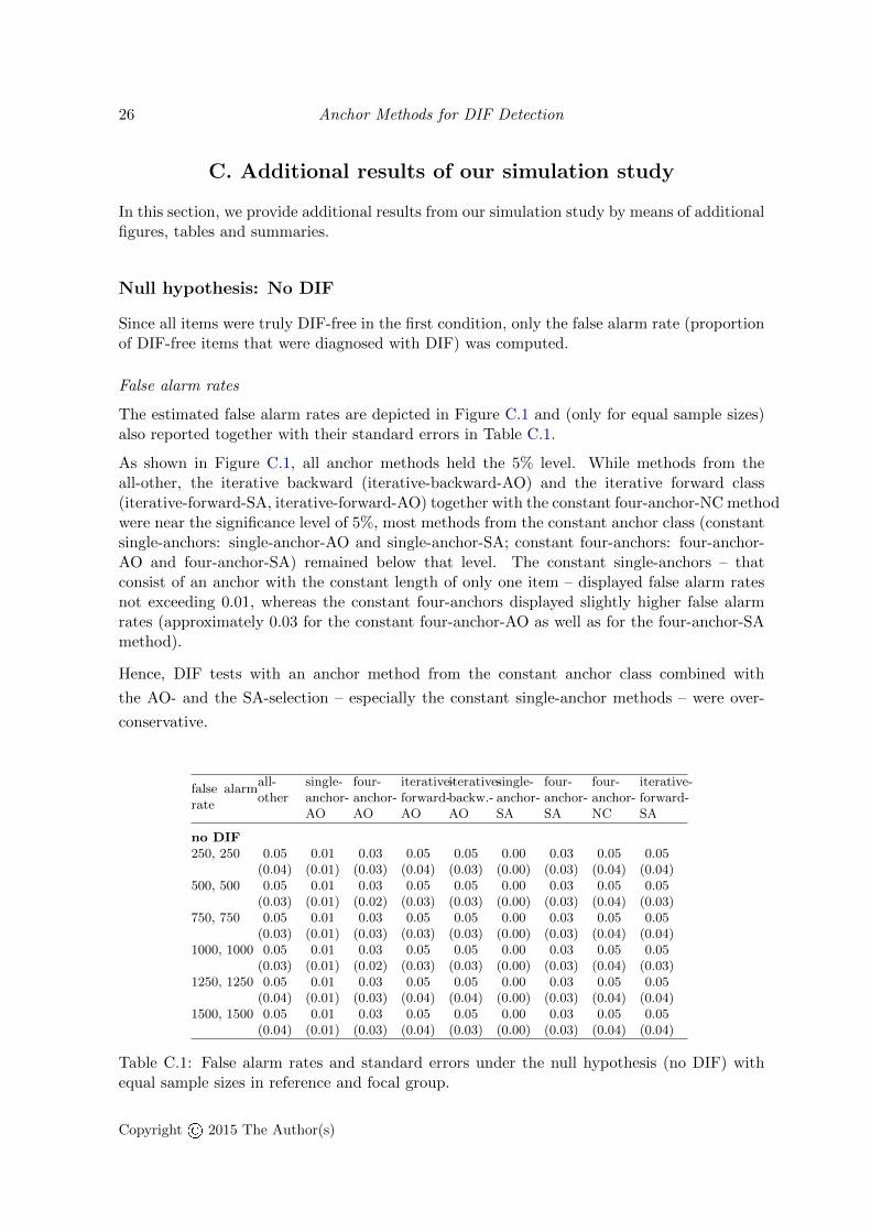
26 Anchor Methods for DIF Detection
C. Additional results of our simulation study
In this section, we provide additional results from our simulation study by means of additionalfigures, tables and summaries.
Null hypothesis: No DIF
Since all items were truly DIF-free in the first condition, only the false alarm rate (proportionof DIF-free items that were diagnosed with DIF) was computed.
False alarm rates
The estimated false alarm rates are depicted in Figure C.1 and (only for equal sample sizes)also reported together with their standard errors in Table C.1.
As shown in Figure C.1, all anchor methods held the 5% level. While methods from theall-other, the iterative backward (iterative-backward-AO) and the iterative forward class(iterative-forward-SA, iterative-forward-AO) together with the constant four-anchor-NC methodwere near the significance level of 5%, most methods from the constant anchor class (constantsingle-anchors: single-anchor-AO and single-anchor-SA; constant four-anchors: four-anchor-AO and four-anchor-SA) remained below that level. The constant single-anchors – thatconsist of an anchor with the constant length of only one item – displayed false alarm ratesnot exceeding 0.01, whereas the constant four-anchors displayed slightly higher false alarmrates (approximately 0.03 for the constant four-anchor-AO as well as for the four-anchor-SAmethod).
Hence, DIF tests with an anchor method from the constant anchor class combined with
the AO- and the SA-selection – especially the constant single-anchor methods – were over-
conservative.
false alarmrate
all-other
single-anchor-AO
four-anchor-AO
iterative-forward-AO
iterative-backw.-AO
single-anchor-SA
four-anchor-SA
four-anchor-NC
iterative-forward-SA
no DIF250, 250 0.05 0.01 0.03 0.05 0.05 0.00 0.03 0.05 0.05
(0.04) (0.01) (0.03) (0.04) (0.03) (0.00) (0.03) (0.04) (0.04)500, 500 0.05 0.01 0.03 0.05 0.05 0.00 0.03 0.05 0.05
(0.03) (0.01) (0.02) (0.03) (0.03) (0.00) (0.03) (0.04) (0.03)750, 750 0.05 0.01 0.03 0.05 0.05 0.00 0.03 0.05 0.05
(0.03) (0.01) (0.03) (0.03) (0.03) (0.00) (0.03) (0.04) (0.04)1000, 1000 0.05 0.01 0.03 0.05 0.05 0.00 0.03 0.05 0.05
(0.03) (0.01) (0.02) (0.03) (0.03) (0.00) (0.03) (0.04) (0.03)1250, 1250 0.05 0.01 0.03 0.05 0.05 0.00 0.03 0.05 0.05
(0.04) (0.01) (0.03) (0.04) (0.04) (0.00) (0.03) (0.04) (0.04)1500, 1500 0.05 0.01 0.03 0.05 0.05 0.00 0.03 0.05 0.05
(0.04) (0.01) (0.03) (0.04) (0.03) (0.00) (0.03) (0.04) (0.04)
Table C.1: False alarm rates and standard errors under the null hypothesis (no DIF) withequal sample sizes in reference and focal group.
Copyright© 2015 The Author(s)
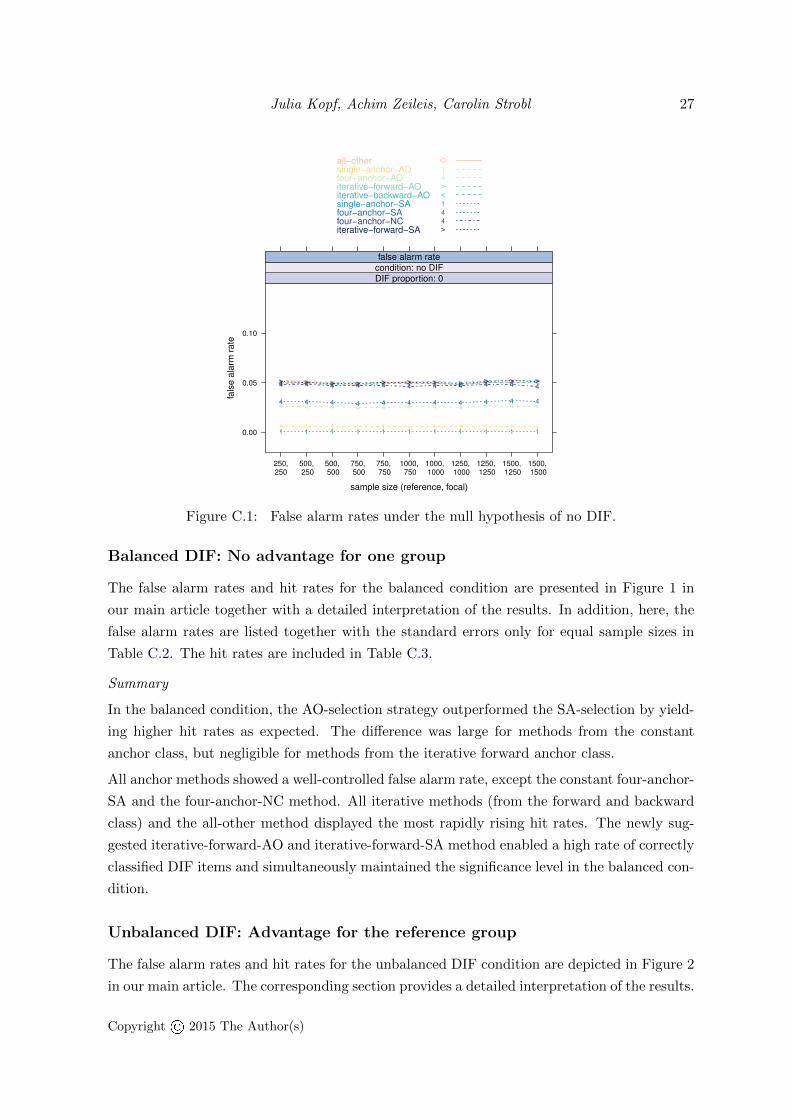
Julia Kopf, Achim Zeileis, Carolin Strobl 27
sample size (reference, focal)
fals
e a
larm
ra
te
0.00
0.05
0.10
250,250
500, 250
500, 500
750, 500
750, 750
1000, 750
1000, 1000
1250, 1000
1250, 1250
1500, 1250
1500, 1500
1 1 1 1 1 1 1 1 1 1 1
4 4 4 4 4 4 4 4 4 4 4
> > > > > > > > > > >< < < < < < < < < < <
1 1 1 1 1 1 1 1 1 1 1
4 4 4 4 4 4 4 4 4 4 4
4 4 4 4 4 4 4 4 4 4 4> > > > > > > > > > >
DIF proportion: 0
condition: no DIF
false alarm rate
all−othersingle−anchor−AOfour−anchor−AOiterative−forward−AOiterative−backward−AOsingle−anchor−SAfour−anchor−SAfour−anchor−NCiterative−forward−SA
1
4
><
1
4
4
>
Figure C.1: False alarm rates under the null hypothesis of no DIF.
Balanced DIF: No advantage for one group
The false alarm rates and hit rates for the balanced condition are presented in Figure 1 in
our main article together with a detailed interpretation of the results. In addition, here, the
false alarm rates are listed together with the standard errors only for equal sample sizes in
Table C.2. The hit rates are included in Table C.3.
Summary
In the balanced condition, the AO-selection strategy outperformed the SA-selection by yield-
ing higher hit rates as expected. The difference was large for methods from the constant
anchor class, but negligible for methods from the iterative forward anchor class.
All anchor methods showed a well-controlled false alarm rate, except the constant four-anchor-
SA and the four-anchor-NC method. All iterative methods (from the forward and backward
class) and the all-other method displayed the most rapidly rising hit rates. The newly sug-
gested iterative-forward-AO and iterative-forward-SA method enabled a high rate of correctly
classified DIF items and simultaneously maintained the significance level in the balanced con-
dition.
Unbalanced DIF: Advantage for the reference group
The false alarm rates and hit rates for the unbalanced DIF condition are depicted in Figure 2
in our main article. The corresponding section provides a detailed interpretation of the results.
Copyright© 2015 The Author(s)
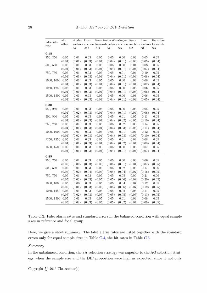
28 Anchor Methods for DIF Detection
false alarmrate
all-other
single-anchor-AO
four-anchor-AO
iterative-forward-AO
iterative-backw.-AO
single-anchor-SA
four-anchor-SA
four-anchor-NC
iterative-forward-SA
0.15250, 250 0.05 0.01 0.03 0.05 0.05 0.00 0.03 0.05 0.05
(0.04) (0.01) (0.03) (0.04) (0.04) (0.01) (0.03) (0.05) (0.04)500, 500 0.05 0.01 0.03 0.05 0.05 0.00 0.04 0.08 0.05
(0.04) (0.01) (0.03) (0.04) (0.04) (0.01) (0.04) (0.07) (0.04)750, 750 0.05 0.01 0.03 0.05 0.05 0.01 0.04 0.10 0.05
(0.04) (0.01) (0.03) (0.04) (0.04) (0.01) (0.04) (0.08) (0.04)1000, 1000 0.05 0.01 0.03 0.05 0.05 0.00 0.04 0.08 0.05
(0.04) (0.01) (0.03) (0.04) (0.04) (0.01) (0.04) (0.07) (0.04)1250, 1250 0.05 0.01 0.03 0.05 0.05 0.00 0.03 0.06 0.05
(0.04) (0.01) (0.03) (0.04) (0.04) (0.01) (0.03) (0.06) (0.04)1500, 1500 0.05 0.01 0.03 0.05 0.05 0.00 0.03 0.06 0.05
(0.04) (0.01) (0.03) (0.04) (0.04) (0.01) (0.03) (0.05) (0.04)
0.30250, 250 0.05 0.01 0.03 0.05 0.05 0.00 0.03 0.05 0.05
(0.04) (0.02) (0.03) (0.04) (0.04) (0.01) (0.04) (0.06) (0.04)500, 500 0.05 0.01 0.03 0.05 0.05 0.01 0.05 0.11 0.05
(0.04) (0.01) (0.03) (0.04) (0.04) (0.02) (0.05) (0.10) (0.04)750, 750 0.05 0.01 0.03 0.05 0.05 0.02 0.06 0.14 0.05
(0.04) (0.01) (0.03) (0.04) (0.04) (0.03) (0.05) (0.11) (0.04)1000, 1000 0.05 0.01 0.03 0.05 0.05 0.01 0.04 0.12 0.05
(0.04) (0.02) (0.03) (0.04) (0.04) (0.03) (0.05) (0.10) (0.04)1250, 1250 0.05 0.01 0.03 0.05 0.05 0.01 0.04 0.08 0.05
(0.04) (0.01) (0.03) (0.04) (0.04) (0.02) (0.04) (0.08) (0.04)1500, 1500 0.05 0.01 0.03 0.05 0.05 0.00 0.03 0.07 0.05
(0.04) (0.01) (0.03) (0.04) (0.04) (0.01) (0.04) (0.07) (0.04)
0.45250, 250 0.05 0.01 0.03 0.05 0.05 0.00 0.03 0.06 0.05
(0.05) (0.02) (0.03) (0.05) (0.05) (0.01) (0.04) (0.07) (0.05)500, 500 0.05 0.01 0.03 0.05 0.05 0.02 0.06 0.17 0.06
(0.05) (0.02) (0.04) (0.05) (0.05) (0.04) (0.07) (0.16) (0.05)750, 750 0.05 0.01 0.03 0.05 0.05 0.05 0.09 0.21 0.06
(0.05) (0.02) (0.03) (0.05) (0.05) (0.06) (0.08) (0.20) (0.05)1000, 1000 0.05 0.00 0.03 0.05 0.05 0.04 0.07 0.17 0.05
(0.05) (0.01) (0.03) (0.05) (0.05) (0.06) (0.07) (0.19) (0.05)1250, 1250 0.05 0.01 0.03 0.05 0.05 0.02 0.05 0.11 0.05
(0.05) (0.02) (0.03) (0.05) (0.05) (0.05) (0.05) (0.13) (0.05)1500, 1500 0.05 0.01 0.03 0.05 0.05 0.01 0.04 0.08 0.05
(0.05) (0.02) (0.03) (0.05) (0.05) (0.02) (0.04) (0.09) (0.05)
Table C.2: False alarm rates and standard errors in the balanced condition with equal samplesizes in reference and focal group.
Here, we give a short summary. The false alarm rates are listed together with the standard
errors only for equal sample sizes in Table C.4, the hit rates in Table C.5.
Summary
In the unbalanced condition, the SA-selection strategy was superior to the AO-selection strat-
egy when the sample size and the DIF proportion were high as expected, since it not only
Copyright© 2015 The Author(s)
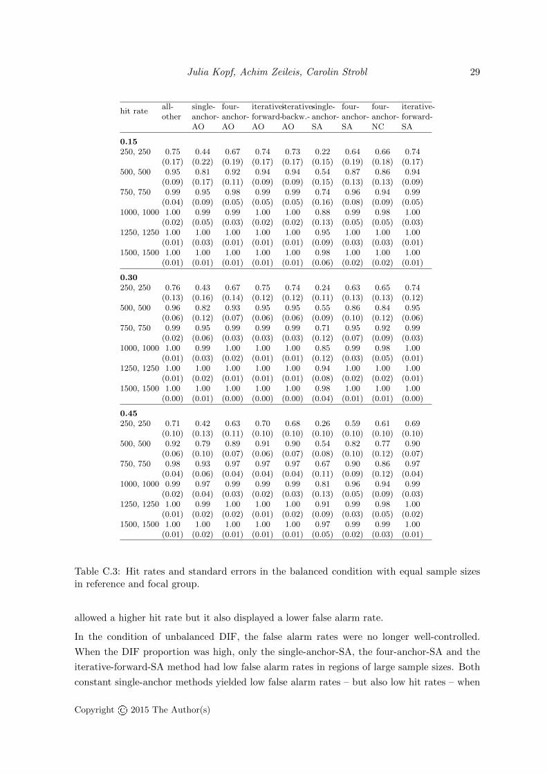
Julia Kopf, Achim Zeileis, Carolin Strobl 29
hit rateall-other
single-anchor-AO
four-anchor-AO
iterative-forward-AO
iterative-backw.-AO
single-anchor-SA
four-anchor-SA
four-anchor-NC
iterative-forward-SA
0.15250, 250 0.75 0.44 0.67 0.74 0.73 0.22 0.64 0.66 0.74
(0.17) (0.22) (0.19) (0.17) (0.17) (0.15) (0.19) (0.18) (0.17)500, 500 0.95 0.81 0.92 0.94 0.94 0.54 0.87 0.86 0.94
(0.09) (0.17) (0.11) (0.09) (0.09) (0.15) (0.13) (0.13) (0.09)750, 750 0.99 0.95 0.98 0.99 0.99 0.74 0.96 0.94 0.99
(0.04) (0.09) (0.05) (0.05) (0.05) (0.16) (0.08) (0.09) (0.05)1000, 1000 1.00 0.99 0.99 1.00 1.00 0.88 0.99 0.98 1.00
(0.02) (0.05) (0.03) (0.02) (0.02) (0.13) (0.05) (0.05) (0.03)1250, 1250 1.00 1.00 1.00 1.00 1.00 0.95 1.00 1.00 1.00
(0.01) (0.03) (0.01) (0.01) (0.01) (0.09) (0.03) (0.03) (0.01)1500, 1500 1.00 1.00 1.00 1.00 1.00 0.98 1.00 1.00 1.00
(0.01) (0.01) (0.01) (0.01) (0.01) (0.06) (0.02) (0.02) (0.01)
0.30250, 250 0.76 0.43 0.67 0.75 0.74 0.24 0.63 0.65 0.74
(0.13) (0.16) (0.14) (0.12) (0.12) (0.11) (0.13) (0.13) (0.12)500, 500 0.96 0.82 0.93 0.95 0.95 0.55 0.86 0.84 0.95
(0.06) (0.12) (0.07) (0.06) (0.06) (0.09) (0.10) (0.12) (0.06)750, 750 0.99 0.95 0.99 0.99 0.99 0.71 0.95 0.92 0.99
(0.02) (0.06) (0.03) (0.03) (0.03) (0.12) (0.07) (0.09) (0.03)1000, 1000 1.00 0.99 1.00 1.00 1.00 0.85 0.99 0.98 1.00
(0.01) (0.03) (0.02) (0.01) (0.01) (0.12) (0.03) (0.05) (0.01)1250, 1250 1.00 1.00 1.00 1.00 1.00 0.94 1.00 1.00 1.00
(0.01) (0.02) (0.01) (0.01) (0.01) (0.08) (0.02) (0.02) (0.01)1500, 1500 1.00 1.00 1.00 1.00 1.00 0.98 1.00 1.00 1.00
(0.00) (0.01) (0.00) (0.00) (0.00) (0.04) (0.01) (0.01) (0.00)
0.45250, 250 0.71 0.42 0.63 0.70 0.68 0.26 0.59 0.61 0.69
(0.10) (0.13) (0.11) (0.10) (0.10) (0.10) (0.10) (0.10) (0.10)500, 500 0.92 0.79 0.89 0.91 0.90 0.54 0.82 0.77 0.90
(0.06) (0.10) (0.07) (0.06) (0.07) (0.08) (0.10) (0.12) (0.07)750, 750 0.98 0.93 0.97 0.97 0.97 0.67 0.90 0.86 0.97
(0.04) (0.06) (0.04) (0.04) (0.04) (0.11) (0.09) (0.12) (0.04)1000, 1000 0.99 0.97 0.99 0.99 0.99 0.81 0.96 0.94 0.99
(0.02) (0.04) (0.03) (0.02) (0.03) (0.13) (0.05) (0.09) (0.03)1250, 1250 1.00 0.99 1.00 1.00 1.00 0.91 0.99 0.98 1.00
(0.01) (0.02) (0.02) (0.01) (0.02) (0.09) (0.03) (0.05) (0.02)1500, 1500 1.00 1.00 1.00 1.00 1.00 0.97 0.99 0.99 1.00
(0.01) (0.02) (0.01) (0.01) (0.01) (0.05) (0.02) (0.03) (0.01)
Table C.3: Hit rates and standard errors in the balanced condition with equal sample sizesin reference and focal group.
allowed a higher hit rate but it also displayed a lower false alarm rate.
In the condition of unbalanced DIF, the false alarm rates were no longer well-controlled.
When the DIF proportion was high, only the single-anchor-SA, the four-anchor-SA and the
iterative-forward-SA method had low false alarm rates in regions of large sample sizes. Both
constant single-anchor methods yielded low false alarm rates – but also low hit rates – when
Copyright© 2015 The Author(s)
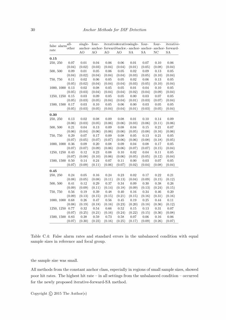
30 Anchor Methods for DIF Detection
false alarmrate
all-other
single-anchor-AO
four-anchor-AO
iterative-forward-AO
iterative-backw.-AO
single-anchor-SA
four-anchor-SA
four-anchor-NC
iterative-forward-SA
0.15250, 250 0.07 0.01 0.04 0.06 0.06 0.01 0.07 0.10 0.06
(0.04) (0.02) (0.03) (0.04) (0.04) (0.01) (0.05) (0.08) (0.04)500, 500 0.09 0.01 0.05 0.06 0.05 0.02 0.09 0.13 0.05
(0.04) (0.02) (0.04) (0.04) (0.04) (0.03) (0.05) (0.10) (0.04)750, 750 0.11 0.02 0.06 0.05 0.05 0.02 0.06 0.13 0.05
(0.05) (0.02) (0.04) (0.04) (0.04) (0.03) (0.05) (0.10) (0.04)1000, 1000 0.13 0.02 0.08 0.05 0.05 0.01 0.04 0.10 0.05
(0.05) (0.03) (0.04) (0.04) (0.04) (0.02) (0.04) (0.09) (0.04)1250, 1250 0.15 0.03 0.09 0.05 0.05 0.00 0.03 0.07 0.05
(0.05) (0.03) (0.05) (0.04) (0.04) (0.01) (0.03) (0.07) (0.04)1500, 1500 0.17 0.03 0.10 0.05 0.06 0.00 0.03 0.05 0.05
(0.05) (0.03) (0.05) (0.04) (0.04) (0.01) (0.03) (0.05) (0.04)
0.30250, 250 0.13 0.02 0.08 0.09 0.08 0.01 0.10 0.14 0.09
(0.06) (0.03) (0.05) (0.06) (0.06) (0.03) (0.06) (0.11) (0.06)500, 500 0.21 0.04 0.13 0.09 0.08 0.04 0.15 0.21 0.07
(0.06) (0.04) (0.06) (0.06) (0.06) (0.05) (0.08) (0.16) (0.06)750, 750 0.29 0.07 0.17 0.09 0.08 0.05 0.13 0.21 0.05
(0.07) (0.05) (0.07) (0.07) (0.06) (0.06) (0.08) (0.18) (0.05)1000, 1000 0.36 0.09 0.20 0.08 0.09 0.04 0.08 0.17 0.05
(0.07) (0.07) (0.09) (0.06) (0.06) (0.07) (0.07) (0.15) (0.04)1250, 1250 0.43 0.12 0.23 0.08 0.10 0.02 0.04 0.11 0.05
(0.07) (0.08) (0.10) (0.06) (0.06) (0.05) (0.05) (0.12) (0.04)1500, 1500 0.50 0.14 0.24 0.07 0.11 0.00 0.03 0.07 0.05
(0.07) (0.09) (0.11) (0.06) (0.07) (0.02) (0.04) (0.08) (0.04)
0.45250, 250 0.24 0.05 0.16 0.24 0.23 0.02 0.17 0.22 0.21
(0.08) (0.05) (0.08) (0.11) (0.13) (0.04) (0.09) (0.15) (0.12)500, 500 0.41 0.12 0.29 0.37 0.34 0.09 0.30 0.38 0.26
(0.09) (0.09) (0.11) (0.14) (0.18) (0.09) (0.13) (0.24) (0.15)750, 750 0.56 0.19 0.39 0.48 0.40 0.16 0.34 0.46 0.20
(0.09) (0.13) (0.15) (0.15) (0.21) (0.15) (0.16) (0.31) (0.16)1000, 1000 0.68 0.26 0.47 0.56 0.45 0.19 0.25 0.44 0.11
(0.08) (0.19) (0.18) (0.16) (0.23) (0.20) (0.18) (0.36) (0.12)1250, 1250 0.77 0.32 0.54 0.66 0.52 0.15 0.13 0.31 0.07
(0.07) (0.25) (0.21) (0.16) (0.24) (0.22) (0.15) (0.36) (0.08)1500, 1500 0.83 0.38 0.59 0.73 0.58 0.07 0.06 0.16 0.06
(0.07) (0.30) (0.23) (0.16) (0.25) (0.17) (0.09) (0.26) (0.07)
Table C.4: False alarm rates and standard errors in the unbalanced condition with equalsample sizes in reference and focal group.
the sample size was small.
All methods from the constant anchor class, especially in regions of small sample sizes, showed
poor hit rates. The highest hit rate – in all settings from the unbalanced condition – occurred
for the newly proposed iterative-forward-SA method.
Copyright© 2015 The Author(s)
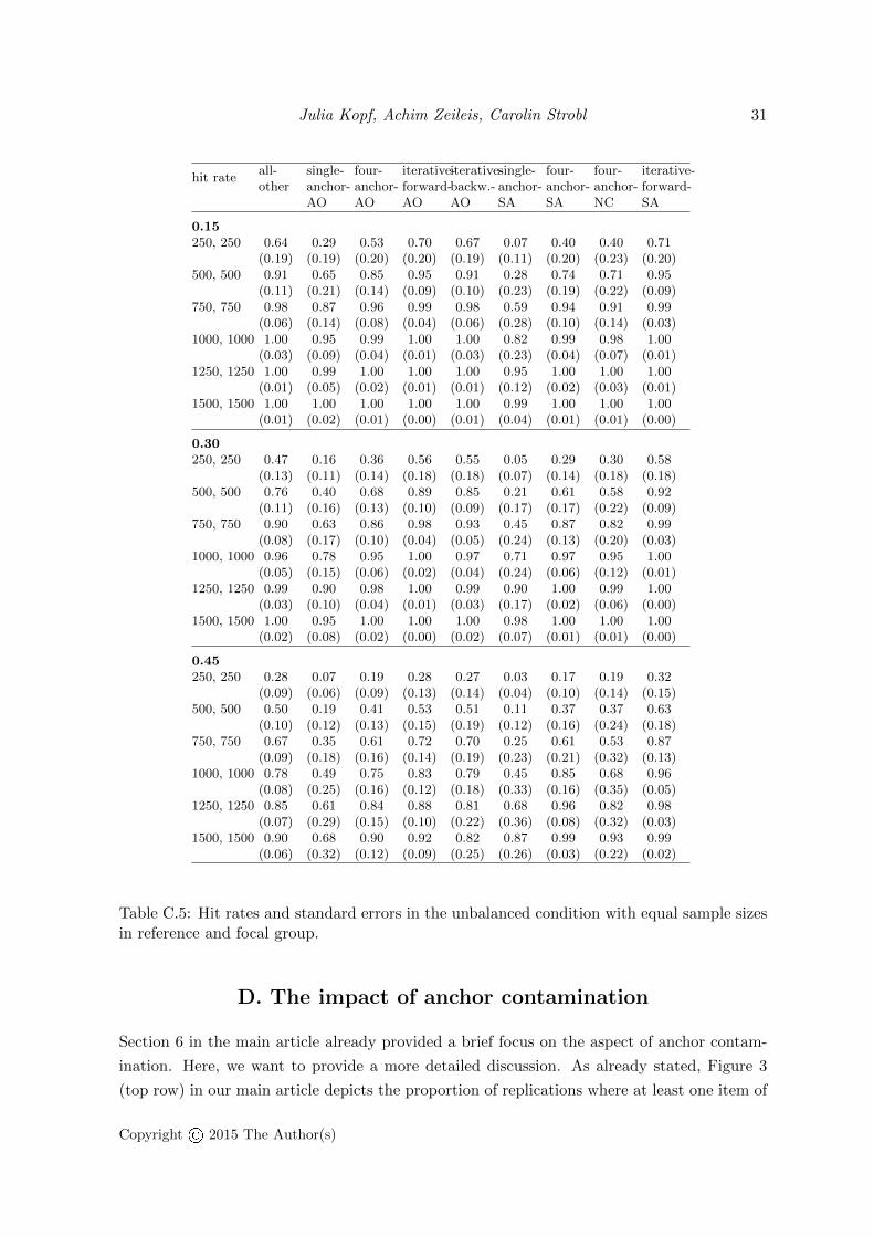
Julia Kopf, Achim Zeileis, Carolin Strobl 31
hit rateall-other
single-anchor-AO
four-anchor-AO
iterative-forward-AO
iterative-backw.-AO
single-anchor-SA
four-anchor-SA
four-anchor-NC
iterative-forward-SA
0.15250, 250 0.64 0.29 0.53 0.70 0.67 0.07 0.40 0.40 0.71
(0.19) (0.19) (0.20) (0.20) (0.19) (0.11) (0.20) (0.23) (0.20)500, 500 0.91 0.65 0.85 0.95 0.91 0.28 0.74 0.71 0.95
(0.11) (0.21) (0.14) (0.09) (0.10) (0.23) (0.19) (0.22) (0.09)750, 750 0.98 0.87 0.96 0.99 0.98 0.59 0.94 0.91 0.99
(0.06) (0.14) (0.08) (0.04) (0.06) (0.28) (0.10) (0.14) (0.03)1000, 1000 1.00 0.95 0.99 1.00 1.00 0.82 0.99 0.98 1.00
(0.03) (0.09) (0.04) (0.01) (0.03) (0.23) (0.04) (0.07) (0.01)1250, 1250 1.00 0.99 1.00 1.00 1.00 0.95 1.00 1.00 1.00
(0.01) (0.05) (0.02) (0.01) (0.01) (0.12) (0.02) (0.03) (0.01)1500, 1500 1.00 1.00 1.00 1.00 1.00 0.99 1.00 1.00 1.00
(0.01) (0.02) (0.01) (0.00) (0.01) (0.04) (0.01) (0.01) (0.00)
0.30250, 250 0.47 0.16 0.36 0.56 0.55 0.05 0.29 0.30 0.58
(0.13) (0.11) (0.14) (0.18) (0.18) (0.07) (0.14) (0.18) (0.18)500, 500 0.76 0.40 0.68 0.89 0.85 0.21 0.61 0.58 0.92
(0.11) (0.16) (0.13) (0.10) (0.09) (0.17) (0.17) (0.22) (0.09)750, 750 0.90 0.63 0.86 0.98 0.93 0.45 0.87 0.82 0.99
(0.08) (0.17) (0.10) (0.04) (0.05) (0.24) (0.13) (0.20) (0.03)1000, 1000 0.96 0.78 0.95 1.00 0.97 0.71 0.97 0.95 1.00
(0.05) (0.15) (0.06) (0.02) (0.04) (0.24) (0.06) (0.12) (0.01)1250, 1250 0.99 0.90 0.98 1.00 0.99 0.90 1.00 0.99 1.00
(0.03) (0.10) (0.04) (0.01) (0.03) (0.17) (0.02) (0.06) (0.00)1500, 1500 1.00 0.95 1.00 1.00 1.00 0.98 1.00 1.00 1.00
(0.02) (0.08) (0.02) (0.00) (0.02) (0.07) (0.01) (0.01) (0.00)
0.45250, 250 0.28 0.07 0.19 0.28 0.27 0.03 0.17 0.19 0.32
(0.09) (0.06) (0.09) (0.13) (0.14) (0.04) (0.10) (0.14) (0.15)500, 500 0.50 0.19 0.41 0.53 0.51 0.11 0.37 0.37 0.63
(0.10) (0.12) (0.13) (0.15) (0.19) (0.12) (0.16) (0.24) (0.18)750, 750 0.67 0.35 0.61 0.72 0.70 0.25 0.61 0.53 0.87
(0.09) (0.18) (0.16) (0.14) (0.19) (0.23) (0.21) (0.32) (0.13)1000, 1000 0.78 0.49 0.75 0.83 0.79 0.45 0.85 0.68 0.96
(0.08) (0.25) (0.16) (0.12) (0.18) (0.33) (0.16) (0.35) (0.05)1250, 1250 0.85 0.61 0.84 0.88 0.81 0.68 0.96 0.82 0.98
(0.07) (0.29) (0.15) (0.10) (0.22) (0.36) (0.08) (0.32) (0.03)1500, 1500 0.90 0.68 0.90 0.92 0.82 0.87 0.99 0.93 0.99
(0.06) (0.32) (0.12) (0.09) (0.25) (0.26) (0.03) (0.22) (0.02)
Table C.5: Hit rates and standard errors in the unbalanced condition with equal sample sizesin reference and focal group.
D. The impact of anchor contamination
Section 6 in the main article already provided a brief focus on the aspect of anchor contam-
ination. Here, we want to provide a more detailed discussion. As already stated, Figure 3
(top row) in our main article depicts the proportion of replications where at least one item of
Copyright© 2015 The Author(s)
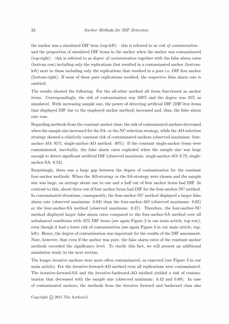
32 Anchor Methods for DIF Detection
the anchor was a simulated DIF item (top-left) – this is referred to as risk of contamination –
and the proportion of simulated DIF items in the anchor when the anchor was contaminated
(top-right) – this is referred to as degree of contamination together with the false alarm rates
(bottom row) including only the replications that resulted in a contaminated anchor (bottom-
left) next to those including only the replications that resulted in a pure i.e. DIF-free anchor
(bottom-right). If none of these pure replications resulted, the respective false alarm rate is
omitted.
The results showed the following: For the all-other method all items functioned as anchor
items. Correspondingly, the risk of contamination was 100% and the degree was 45% as
simulated. With increasing sample size, the power of detecting artificial DIF (DIF-free items
that displayed DIF due to the employed anchor method) increased and, thus, the false alarm
rate rose.
Regarding methods from the constant anchor class, the risk of contaminated anchors decreased
when the sample size increased for the SA- or the NC-selection strategy, while the AO-selection
strategy showed a relatively constant risk of contaminated anchors (observed maximum: four-
anchor-AO: 91%, single-anchor-AO method: 40%). If the constant single-anchor items were
contaminated, inevitably, the false alarm rates exploded when the sample size was large
enough to detect significant artificial DIF (observed maximum: single-anchor-AO: 0.72, single-
anchor-SA: 0.52).
Surprisingly, there was a large gap between the degree of contamination for the constant
four-anchor methods: When the AO-strategy or the SA-strategy were chosen and the sample
size was large, on average about one to one and a half out of four anchor items had DIF. In
contrast to this, about three out of four anchor items had DIF for the four-anchor-NC method.
In contaminated situations, consequently, the four-anchor-NC method displayed a larger false
alarm rate (observed maximum: 0.83) than the four-anchor-AO (observed maximum: 0.65)
or the four-anchor-SA method (observed maximum: 0.37). Therefore, the four-anchor-NC
method displayed larger false alarm rates compared to the four-anchor-SA method over all
unbalanced conditions with 45% DIF items (see again Figure 2 in our main article, top row),
even though it had a lower risk of contamination (see again Figure 3 in our main article, top-
left). Hence, the degree of contamination was important for the results of the DIF assessment.
Note, however, that even if the anchor was pure, the false alarm rates of the constant anchor
methods exceeded the significance level. To clarify this fact, we will present an additional
simulation study in the next section.
The longer iterative anchors were more often contaminated, as expected (see Figure 3 in our
main article). For the iterative-forward-AO method even all replications were contaminated.
The iterative-forward-SA and the iterative-backward-AO method yielded a risk of contam-
ination that decreased with the sample size (observed minimum: 0.42 and 0.89). In case
of contaminated anchors, the methods from the iterative forward and backward class also
Copyright© 2015 The Author(s)
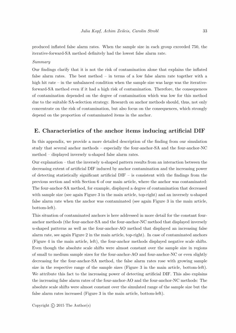
Julia Kopf, Achim Zeileis, Carolin Strobl 33
produced inflated false alarm rates. When the sample size in each group exceeded 750, the
iterative-forward-SA method definitely had the lowest false alarm rate.
Summary
Our findings clarify that it is not the risk of contamination alone that explains the inflated
false alarm rates. The best method – in terms of a low false alarm rate together with a
high hit rate – in the unbalanced condition when the sample size was large was the iterative-
forward-SA method even if it had a high risk of contamination. Therefore, the consequences
of contamination depended on the degree of contamination which was low for this method
due to the suitable SA-selection strategy. Research on anchor methods should, thus, not only
concentrate on the risk of contamination, but also focus on the consequences, which strongly
depend on the proportion of contaminated items in the anchor.
E. Characteristics of the anchor items inducing artificial DIF
In this appendix, we provide a more detailed description of the finding from our simulation
study that several anchor methods – especially the four-anchor-SA and the four-anchor-NC
method – displayed inversely u-shaped false alarm rates.
Our explanation – that the inversely u-shaped pattern results from an interaction between the
decreasing extent of artificial DIF induced by anchor contamination and the increasing power
of detecting statistically significant artificial DIF – is consistent with the findings from the
previous section and with Section 6 of our main article, where the anchor was contaminated:
The four-anchor-SA method, for example, displayed a degree of contamination that decreased
with sample size (see again Figure 3 in the main article, top-right) and an inversely u-shaped
false alarm rate when the anchor was contaminated (see again Figure 3 in the main article,
bottom-left).
This situation of contaminated anchors is here addressed in more detail for the constant four-
anchor methods (the four-anchor-SA and the four-anchor-NC method that displayed inversely
u-shaped patterns as well as the four-anchor-AO method that displayed an increasing false
alarm rate, see again Figure 2 in the main article, top-right). In case of contaminated anchors
(Figure 4 in the main article, left), the four-anchor methods displayed negative scale shifts.
Even though the absolute scale shifts were almost constant over the sample size in regions
of small to medium sample sizes for the four-anchor-AO and four-anchor-NC or even slightly
decreasing for the four-anchor-SA method, the false alarm rates rose with growing sample
size in the respective range of the sample sizes (Figure 3 in the main article, bottom-left).
We attribute this fact to the increasing power of detecting artificial DIF. This also explains
the increasing false alarm rates of the four-anchor-AO and the four-anchor-NC methods: The
absolute scale shifts were almost constant over the simulated range of the sample size but the
false alarm rates increased (Figure 3 in the main article, bottom-left).
Copyright© 2015 The Author(s)
34 Anchor Methods for DIF Detection
For the four-anchor-SA method the absolute scale shift also decreased with increasing sample
size in regions of medium or large sample sizes (Figure 4 in our main article, left) and so did
the false alarm rate in the respective range of the sample sizes (Figure 3 in our main article,
bottom-left).
However, in case of pure replications, the scale shift of the benchmark method was fluctuat-
ing around zero, whereas the scale shift of all remaining constant four-anchor methods was
negative (Figure 4 in our main article, right) and decreasing with the sample size.
These findings explain why the u-shaped patterns occurred for the four-anchor-SA and the
four-anchor-NC method: These methods were able to reduce the absolute scale shift with
increasing sample size because the scale shift in pure replications reduced and the risk of
contamination reduced as well (i.e. the number of pure replications increased). Taking the
increasing power of detecting artificial DIF with growing sample size into account, an inversely
u-shaped pattern resulted for the false alarm rates. In contrast to this, the four-anchor-AO
method always displayed a relatively high scale shift (that only reduced slightly when the
anchor was pure). The power of detecting artificial DIF increased with growing sample size
and, therefore, the false alarm rate showed an increase and no considerable decrease.
Summary
In summary, the interaction between a decreasing extent of artificial DIF and an increasing
statistical power to detect artificial DIF with growing sample size resulted in an inversely
u-shaped false alarm rate. The risk and degree of contamination alone cannot explain the
presence of artificial DIF. The anchor items selected by certain anchor selection strategies
differed systematically from randomly chosen pure anchor items even if the located anchor
items were by definition DIF-free. Counterintuitively instead of items with small differences,
these methods tended to select exactly those items with large differences. Therefore, the
anchor items found by the SA-, the NC- or the AO-selection strategy displayed a negative
scale shift in the additional simulation study and, thus, shifted the scales apart and induced
artificial DIF.
This implies that not only the risk and the degree of contamination but also the scale shift in
by definition pure replications should be regarded when anchor methods are developed and
investigated in simulation studies. Otherwise, inflated false alarm rates might occur even if
the anchor is pure.
F. Summary and discussion
Practical recommendations
Our simulation study highlights the importance of the anchor selection for the correct classi-
fication of DIF and DIF-free items and the necessity of a careful consideration of the anchor
Copyright© 2015 The Author(s)
Julia Kopf, Achim Zeileis, Carolin Strobl 35
method to avoid high misclassification rates and doubtful test results.
In case of balanced DIF, the all-other method was slightly better than the iterative-forward-
SA strategy. However, due to the fact that the all-other method resulted in seriously inflated
false alarm rates when the situation was unbalanced – and that it is doubtful whether the
situation of balanced DIF is ever met in practice (Wang and Yeh 2003; Wang et al. 2012) –
the usage of this anchor method is inadvisable.
Thus, the newly suggested iterative-forward-SA strategy is recommended. When the sample
size was large enough, the false alarm rates were low in any condition even if the anchor was
contaminated and the hit rates grew rapidly. The adequacy of the selection strategies – by
single-anchor (SA) or by all-other (AO) – depended on the DIF situation. In the balanced
condition, the AO-selection strategy performed suitable, whereas in the unbalanced condition
the SA-selection strategy was more appropriate. But when the iterative-forward class was
used, the advance of the AO-selection strategy was marginal. Therefore, we recommend the
newly suggested iterative-forward-SA method over the iterative-forward-AO method.
Future research
While our research was limited to DIF detection in the Rasch model using the Wald test,
future research may investigate the usefulness of the iterative-forward-SA method for other
IRT models and combine it with other DIF detection methods.
In particular, it would be interesting to explore the possibility of employing the iterative-
forward strategy together with other IRT-based tests, such as the widely used (see, e.g.,
Woods 2009; Gonzalez-Betanzos and Abad 2012) likelihood ratio test, and investigate its
compatibility with non-IRT based methods. Future research may e.g. investigate whether
those items selected as anchor items by the newly suggested iterative-forward-SA method
with the Wald test (or an alternative DIF test) also provide a useful matching criterion
for non-IRT based tests. The test results could then be compared with those of classical
purification methods that were previously found to improve the final test results (see Miller
and Oshima 1992; Clauser, Mazor, and Hambleton 1993; Navas-Ara and Gomez-Benito 2002,
and the references therein).
When other IRT models were the underlying data generating process, previous research found
highly discriminating items to be better suited as anchor items (Lopez Rivas et al. 2009;
Gonzalez-Betanzos and Abad 2012). Thus, the iterative forward procedure might also be
combined with a minimum discrimination requirement for the anchor candidates.
Furthermore, the iterative forward anchor class with the SA-selection may be compared with
modifications of the anchor selection strategy. For example, Shih and Wang (2009) suggest to
use the items corresponding to the lowest rank of the mean absolute DIF statistics similar to
the rank-based strategy of Woods (2009). Then items are anchor candidates if they display
the lowest mean DIF test statistic when every item is tested for DIF using every other item
Copyright© 2015 The Author(s)
36 Anchor Methods for DIF Detection
as constant single-anchor. This modification may be less affected by sample size. Wang et al.
(2012) established an improvement of the AO-selection strategy by incorporating additional
iterations. Firstly, every item is tested for DIF using the all-other method. Then, iteratively,
DIF items are excluded from the anchor candidates and a new DIF analysis using the current
anchor is conducted until two steps reach the same results. Finally, the anchor items are
selected from the remaining candidates using the rank-based strategy. Future research could
compare the improved AO-selection to the SA-selection strategy.
Moreover, the DIF test results may also be improved by the construction of new anchor
selection strategies. Ideally, the anchor items are DIF-free and induce no artificial scale shift.
Furthermore, the impact of the degree of contamination is important for the appropriateness
of the results in DIF detection. Therefore, improving the anchor selection strategies with the
aim to locate anchors with a small degree of contamination remains an important task.
Affiliation:
Julia KopfDepartment of StatisticsLudwig-Maximilians-Universitat MunchenLudwigstraße 3380539 Munchen, GermanyE-mail: [email protected]
Achim ZeileisDepartment of StatisticsFaculty of Economics and StatisticsUniversitat InnsbruckUniversitatsstraße 156020 Innsbruck, AustriaE-mail: [email protected]: http://eeecon.uibk.ac.at/~zeileis/
Carolin StroblDepartment of PsychologyUniversitat ZurichBinzmuhlestrasse 148050 Zurich, SwitzerlandE-mail: [email protected]
Copyright© 2015 The Author(s)