A formulation of a mathematical model for the induction ...geuzaine/preprints/preprint_aphi_nonlin.pdf · Journal of Computational Physics 00 (2016) 1–20 A- formulation of a mathematical

Journal of Computational Physics 00 (2016) 1–20

A-� formulation of a mathematical model for the inductionhardening process with a nonlinear law for the magnetic field

Jaroslav Chovana, Christophe Geuzaineb, Marian Slodickaa

aDepartment of Mathematical Analysis, Ghent University, Galglaan 2, 9000 Ghent, BelgiumbDepartment of Electrical Engineering and Computer Science, University of Liege, Montefiore Institute B28, Sart Tilman Campus, Allee de la

Decouverte 10, B-4000 Liege, Belgium

AbstractWe derive and analyse a mathematical model for induction hardening. We assume a nonlinear relation between the magnetic

field and the magnetic induction field. For the electromagnetic part, we use the vector-scalar potential formulation.The coupling between the electromagnetic and the thermal part is provided through the temperature-dependent electric con-

ductivity and the joule heating term, the most crucial element, considering the mathematical analysis of the model. It acts as asource of heat in the thermal part and leads to the increase in temperature. Therefore, in order to be able to control it, we apply atruncation function.

Using Rothe’s method, we prove the existence of a global solution to the whole system. The nonlinearity in the electromagneticpart is handled by the theory of monotone operators.

c� 2015 Published by Elsevier Ltd.

Keywords: Maxwell’s equations, Minty-Browder, Monotone operators, Rothe’s method, Scalar potential, Vector potential2010 MSC: 35K61, 35Q61, 35Q79, 65M12

1. Introduction

There are many papers dealing with mathematical models of the induction hardening process. Some of themprovide various numerical schemes e.g. [1, 2, 3, 4, 5, 6]. But they omit mathematical or numerical analysis of theirmodels and numerical schemes. Other papers deal with the well-posedness of the problem and provide theoreticalresults e.g. [7, 8, 9, 10, 11]. The topic of induction hardening has been broadly covered in papers [12, 13] and [14].However, all manuscripts tackling the theoretical side of the induction hardening phenomena present mathematicalmodels with linear dependency between magnetic and magnetic induction field. The paper [15] studied a mathematicalmodel with a nonlinear relation between those two vectorial fields (which better reflects reality), but the study wasrestricted just to a conductor. The authors proved solvability for a formulation with magnetic induction field as anunknown. We present the vector-scalar potential formulation for a nonlinear setting including conducting and non-conducting parts. This means that material coe�cients may have jumps across the interfaces. To our best knowledgenothing similar has been done before.

Email addresses: [email protected] (Jaroslav Chovan), [email protected] (Christophe Geuzaine),[email protected] (Marian Slodicka)

URL: http://cage.ugent.be/~jchovan (Jaroslav Chovan), http://montefiore.ulg.ac.be/~geuzaine (Christophe Geuzaine),http://cage.ugent.be/~ms (Marian Slodicka)

1

J. Chovan, Ch. Geuzaine & M. Slodicka / Journal of Computational Physics 00 (2016) 1–20 2

1.1. Derivation of a mathematical model

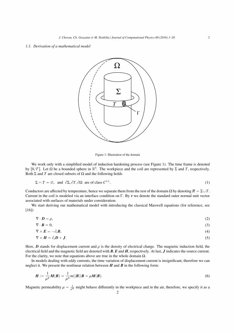
Figure 1: Illustration of the domain

We work only with a simplified model of induction hardening process (see Figure 1). The time frame is denotedby r0,T s. Let ⌦ be a bounded sphere in R3. The workpiece and the coil are represented by ⌃ and T , respectively.Both ⌃ and T are closed subsets of ⌦ and the following holds

⌃X T “ ?, and B⌃, BT, B⌦ are of class C1,1. (1)

Conductors are a↵ected by temperature, hence we separate them from the rest of the domain⌦ by denoting⇡ “ ⌃YT .Current in the coil is modeled via an interface condition on �. By ⌫ we denote the standard outer normal unit vectorassociated with surfaces of materials under consideration.

We start deriving our mathematical model with introducing the classical Maxwell equations (for reference, see[16])

r ¨ D “ ⇢, (2)

r ¨ B “ 0, (3)

rˆ E “ ´Bt B, (4)

rˆ H “ Bt D ` J. (5)

Here, D stands for displacement current and ⇢ is the density of electrical charge. The magnetic induction field, theelectrical field and the magnetic field are denoted with B, E and H, respectively. At last, J indicates the source current.For the clarity, we note that equations above are true in the whole domain ⌦.

In models dealing with eddy currents, the time variation of displacement current is insignificant, therefore we canneglect it. We present the nonlinear relation between H and B in the following form:

H :“ 1µ˚ MpBq “ 1

µ˚ mp|B|qB “ µMpBq. (6)

Magnetic permeability µ “ 1µ˚ might behave di↵erently in the workpiece and in the air, therefore, we specify it as a

2


split function

µpxq “"µ⇡pxq, if x P ⇡,µApxq, if x P ⌦z⇡. (7)

Both µ⇡ and µA are strictly positive and bounded. There is no jump in the tangential component of H along theboundaries between di↵erent materials, i.e.

rµMprˆ Aq ˆ ⌫sB⇡ “ 0.

The vectorial field M is supposed to be potential i.e. grad �M “ M, cf. [17] . Its potential is denoted by �M .Moreover, we assume that M is strictly monotone and Lipschitz continuous. Furthermore, we introduce Ohm’s law

J “ �E. (8)

Function � represents the electric conductivity and it is defined as follows

�pupx, tqq “"�⇡pupx, tqq, if x P ⇡, t P r0,T s,0, if x P ⌦z⇡, t P r0,T s, (9)

where upx, tq is a function of temperature in the workpiece and the coil. We consider � to be continuous, bounded andstrictly positive in ⇡. Since ⌦ is a simply-connected domain and (3) is true in the whole ⌦, we can use ([18, Theorem3.6]) to obtain exactly one magnetic vector potential A P Hpcurl ;⌦q with the following properties:

B “ rˆ A, r ¨ A “ 0, A ˆ ⌫ “ 0 on B⌦. (10)

Substituting (10) into (4) we get

rˆ pE ` Bt Aq “ 0 in ⌦. (11)

Using (11), we can apply ([18, Theorem 2.9]) to acquire a unique scalar potential � P H1p⌦q{R such that:

E ` Bt A “ ´r�. (12)

Combining (12),(10),(8),(6) and (5), we arrive at the following boundary value problem for vector potential A:

�Bt A ` rˆ µMprˆ Aq ` ��Tr� “ 0 for a.e. px, tq P ⌦ˆ p0,T q :“ QT ,

A ˆ ⌫ “ 0 for a.e. px, tq P B⌦ˆ p0,T q,Ap0q “ A0 for x P ⌦, t “ 0.

(13)

Characteristic function �T has value 1, if x P T and 0 otherwise. We use it, because the external source of the current,which is defined by the gradient of the scalar potential, is present only in the coil (T , see Figure 1).

Scalar potential � is determined by the following elliptic equation with homogenous Neumann boundary conditionon BT and interface condition on �:

´r ¨ p�⇡r�q “ 0 for a.e. px, tq P T ˆ p0,T q,´�⇡ B�

B⌫ “ 0 for a.e. px, tq P BT ˆ p0,T q,”´�⇡ B�

B⌫ı

�“ j for a.e. px, tq P �ˆ p0,T q.

(14)

External source current density is represented by function jpx, tq, which is assumed to be Lipschitz continuous intime. Jump across interface � is indicated by r¨s�.

Eddy currents generated in the workpiece raise temperature by a significant amount. This phenomenon is called

3


Joule heat and it is expressed as

J ¨ E (8)“ �⇡ |E|2 (12)“ �⇡ |Bt A ` �Tr�|2 . (15)

This term is crucial and causes numerous troubles during mathematical treatment (un-boundedness), therefore, weintroduce a cut-o↵ function and work with truncated Joule-heating term.

Rrpxq :“$&

%

r ° 0 if x ° r,x if |x| § r,

´r if x † ´r.(16)

Evolution of temperature in the workpiece and the coil (⇡, see Figure 1) is characterized by the following parabolicnonlinear equation with the homogenous Neumann boundary condition:

Bt�puq ´ r ¨ p�ruq “ Rr

´�⇡ |Bt A ` �Tr�|2

¯for a.e. px, tq P ⇡ˆ p0,T q,

´� BuB⌫ “ 0 for a.e. px, tq P B⇡ˆ p0,T q,

up0q “ u0 for x P ⇡, t “ 0.

(17)

Continuous function �px, tq is supposed to be strictly positive and bounded. The nonlinear function � is of a lineargrowth and its derivative is bounded from below by a positive constant.

Equations (13),(14) and (17) model the process of induction hardening in our simplified domain ⌦. They aretied together through terms r�, � and Bt A. One could ask, whether the artificial intervention in the form of cut-o↵function was correct. In real applications of induction hardening, there is always a switch-o↵ button, which is usedto prevent the workpiece from thermal deformations. When the temperature reaches a certain degree, this button isturned-o↵, the stream of electric current is stopped and the workpiece is cooled down. Therefore, applying the cut-o↵function on Joule-heating term in (17), is actually a simulation of this switch-o↵ button and indeed, necessary to bedone.

2. Functional setting

2.1. Variational formulationLet us start with some basic notations. Through the whole paper we adopt notation p¨, ¨q⌦ for the standard inner

product in L2p⌦q or L2p⌦q. Norm induced by this inner product is indicated as }¨}L2p⌦q. Set of abstract functionsk : r0,T s Ñ Y equipped with the norm max

tPr0,T s}¨}Y is denoted as Cpr0,T s; Yq. In a case when p ° 1, norm in

Lppp0,T q; Yq is defined as´≥T

0 }¨}pY dt

¯ 1p. Set of all � ` c, where � P H1pT q and c is a constant is marked as �c.

Considering the vector potential A, we introduce the Hilbert space

XN,0 “ t' P Hpcurl ;⌦q; r ¨ ' “ 0, and 'ˆ ⌫ “ 0 on B⌦u,where Hpcurl ;⌦q “ t' P L2p⌦q : r ˆ ' P L2p⌦qu. Using Friedrichs’ inequality for vectorial fields (cf. [18,Lemma 3.4] or [19, Cor. 3.51]) we see that we may furnish XN,0 with norm }'}XN,0

:“ }rˆ '}L2p⌦q. Taking intoaccount (1), we can use [18, Theorem 3.7] or [20, Theorem 2.12] to conclude that XN,0 is a closed subspace of H1p⌦q.1Multiplying (13) by a test function ' P XN,0, integrating over ⌦ and using Green’s theorem, we obtain the variationalformulation for vector potential A:

p�⇡Bt A,'q⇡ ` pµMprˆ Aq,rˆ 'q⌦ ` p�⇡r�,'qT “ 0 @' P XN,0. (18)

1The relation XN,0 Ä H1p⌦q is crucial for our mathematical approach. We would like to point out that the same inclusion is valid also forconvex domains (with non smooth boundary). In such a case one can rely on the [20, Theorem 2.17]. All presented results hold true also for convexdomains.

4


For equation (17) we follow identical steps as above, using P H1p⇡q as a test function, which brings us to thevariational formulation for function u:

pBt�puq, q⇡ ` p�ru,r q⇡ “´Rr

´�⇡ |Bt A ` �Tr�|2

¯,

¯

⇡@ P H1p⇡q. (19)

Norm in H1p⇡q is defined as } }2H1p⇡q :“ } }2

L2p⇡q ` }r }2L2p⇡q.

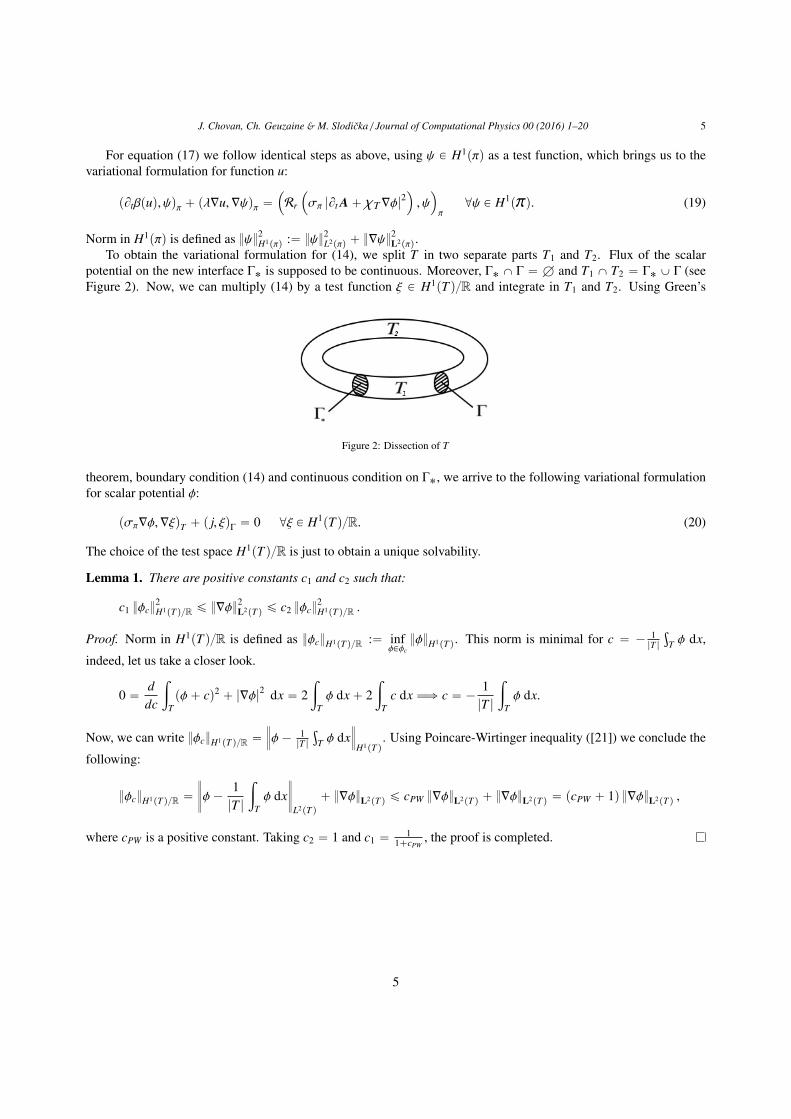
To obtain the variational formulation for (14), we split T in two separate parts T1 and T2. Flux of the scalarpotential on the new interface �˚ is supposed to be continuous. Moreover, �˚ X � “ H and T1 X T2 “ �˚ Y � (seeFigure 2). Now, we can multiply (14) by a test function ⇠ P H1pT q{R and integrate in T1 and T2. Using Green’s

Figure 2: Dissection of T

theorem, boundary condition (14) and continuous condition on �˚, we arrive to the following variational formulationfor scalar potential �:

p�⇡r�,r⇠qT ` p j, ⇠q� “ 0 @⇠ P H1pT q{R. (20)

The choice of the test space H1pT q{R is just to obtain a unique solvability.

Lemma 1. There are positive constants c1 and c2 such that:

c1 }�c}2H1pTq{R § }r�}2

L2pTq § c2 }�c}2H1pTq{R .

Proof. Norm in H1pT q{R is defined as }�c}H1pTq{R :“ inf�P�c

}�}H1pTq. This norm is minimal for c “ ´ 1|T |

≥T � dx,

indeed, let us take a closer look.

0 “ ddc

ª

Tp� ` cq2 ` |r�|2 dx “ 2

ª

T� dx ` 2

ª

Tc dx ùñ c “ ´ 1

|T |ª

T� dx.

Now, we can write }�c}H1pTq{R “›››� ´ 1

|T |≥

T � dx›››

H1pTq. Using Poincare-Wirtinger inequality ([21]) we conclude the

following:

}�c}H1pTq{R “››››� ´ 1

|T |ª

T� dx

››››L2pTq

` }r�}L2pTq § cPW }r�}L2pTq ` }r�}L2pTq “ pcPW ` 1q }r�}L2pTq ,

where cPW is a positive constant. Taking c2 “ 1 and c1 “ 11`cPW

, the proof is completed.

5


2.2. Assumptions

To achieve better clarity and readability of our paper, we list all assumptions altogether:

pa1q 0 † µ⇡˚ § µ⇡pxq § µ⇡˚ † 8 @x P ⌃,pa2q 0 † µA˚ § µApxq § µ˚

A † 8 @x P ⌦z⌃,pbq µ˚ “ min tµ⇡˚, µA˚u, µ˚ “ max

µ⇡˚, µ˚

A

(

pc1q µ P H1p⇡qpc2q µ P H1p⌦z⇡qpdq 0 † �˚ § �pupx, tqq § �˚ † 8 @px, tq P ⇡ˆ p0,T q,

pe1q 0 † �˚ § �px, tq § �˚ † 8 @px, tq P ⇡ˆ p0,T q,pe2q |�px, t2q ´ �px, t1q| § C� |t2 ´ t1| C� ° 0,@x P ⇡,@t2, t1 P r0,T sp f q | jpx, t2q ´ jpx, t1q| § C j |t2 ´ t1| C j ° 0,@x P �,@t2, t1 P r0,T s,pgq j P L2pp0,T q; H´1{2p�qq, ≥

� j d� “ 0,phq u0 P H1

0p⇡q,piq A0 P XN,0,

p jq � is continuous, �p0q “ 0,|�pxq| § C�p1 ` |x|q, 0 † �˚ § �1pxq C� ° 0,@x P R,

pk1q pMpxq ´ Mpyqq ¨ px ´ yq • cM |x ´ y|2 cM ° 0,@x, y P R3,

pk2q |Mpxq ´ Mpyq| § CM |x ´ y| CM ° 0,@x, y P R3,

pk3q Mp0q “ 0.

(21)

Following [17, Theorem 5.1], we can see that potential �M of vectorial field M with properties pk1q ´ pk3q, is strictlyconvex. Applying [17, Theorem 8.4], we get

Mpxq ¨ px ´ yq • �Mpxq ´ �Mpyq @x, y P R3. (22)

Thanks to pk1q and pk2q, we can bound �M from below

�Mpxq “ª 1

0Mpxpq ¨ x dp “

ª 1

0Mpxpq ¨ pxpqp´1 dp •

ª 1

0cM |xp|2 p´1 dp “ cM

2|x|2 (23)

and from above

�Mpxq “ª 1

0Mpxpq ¨ x dp §

ª 1

0|Mpxpq| |x| dp § CM

ª 1

0|xp| |x| dp “ CM

2|x|2 . (24)

3. Existence of a solution

3.1. Time discretization scheme and a priori estimates

In this section we discretize the time interval r0,T s and solve a system of steady-state di↵erential equationson each time step. Afterwards, we construct piece-wise constant and piece-wise linear in time functions and showconvergence of sub-sequences of these functions in appropriate functional spaces to the weak solution. This approachis called Rothe’s method ([22, 23]). Consider a time step ⌧. We split the time interval in n equidistant parts i.e.n⌧ “ T , where n P N. Denoting ti “ i⌧ we can write the following for any function f :

fi “ f ptiq, � fi “ fi ´ fi´1

⌧.

6


Applying this method to the system (18), (19), (20), we are able to approximate it on every time step ti, for i “ 1 . . . n

p��puiq, q⇡ ` p�irui, q⇡ “´Rr

´�⇡pui´1q |�Ai ` �Tr�i|2

¯,

¯

⇡for any P H1p⇡q, (25)

p�⇡pui´1q�Ai,'q⇡ ` pµMprˆ Aiq,rˆ 'q⌦ ` p�⇡pui´1qr�i,'qT “ 0 for any ' P XN,0, (26)

p�⇡pui´1qr�i,r⇠qT ` p ji, ⇠q� “ 0 for any ⇠ P H1pT q{R. (27)

To prove the solvability on each time step, we use the theory of monotone operators (for more details, see [17, 24]).

Lemma 2. Assume that (21) holds. Then, for any i “ 1 . . . n, there exists a uniquely determined triplet �ci P H1pT q{R,Ai P XN,0 and ui P H1p⇡q solving system (25)-(27).

Proof. Let us define operators: F� : XN,0 Ñ pXN,0q˚ and G� : H1p⇡q Ñ pH1p⇡qq˚

⌦F�pAq,'↵ :“ˆ�

A⌧,'

˙

⇡

` pµMprˆ Aq,rˆ 'q⌦ ,⌦G�puq, ↵ :“

ˆ�puq⌧,

˙

⇡

` p�ru,r q⇡ .

Assuming that ⌧ is small enough, i.e. 0 † ⌧ † 1, these operators are strictly monotone, coercive and demicontinuous.Rest of the proof serves as a guideline for obtaining a solution-triplet on every time step t “ ti, for i “ 1 . . . n.Applying Lax-Milgram lemma (see [19, Lemma 2.21]) to (27), we obtain a unique solution �ci P H1p⇡q{R on a timestep t “ ti (ui´1 is known on this time step).

To obtain a unique solution Ai at a time step ti, we have to solve the following identity:

DF�⇡pui´1qpAiq,'

E “ˆ�⇡pui´1q Ai´1

⌧,'

˙

⇡

´ p�⇡pui´1qr�i,'qT .

Since the right-hand side (RHS) is known, we can use [17, Theorem 18.2] to provide the solution. Now, we caninvolve the same theorem again to acquire a unique solution ui P H1p⇡q of the setting below (taking into account thatthe RHS is known)

⌦G�i puiq, ↵ “ˆ�pui´1q

⌧,

˙

⇡

`´Rr

´�⇡pui´1q |�Ai ` �Tr�i|2

¯,

¯

⇡

This provides us with the solution-triplet t�ci , Ai, uiu on a time step t “ ti, for i “ 1 . . . n.

To wrap everything together we state a pseudo-scheme for obtaining the solution-triplet t�ci , Ai, uiu for every timestep t “ ti:

1. Let i be given and assume that ui´1, ji and �i are known

2. Solve: p�⇡pui´1qr�i,r⇠qT ` p ji, ⇠q� “ 0

3. Solve:´�⇡pui´1q Ai

⌧ ,'¯

⇡` pµMprˆ Aiq,rˆ 'q⌦ “

´�⇡pui´1q Ai´1

⌧ ,'¯

⇡´ p�⇡pui´1qr�i,'qT (28)

4. Solve:´�puiq⌧ ,

¯

⇡` p�irui,r q⇡ “

´�pui´1q

⌧ , ¯

⇡`

´Rr

´�⇡pui´1q |�Ai ` �Tr�i|2

¯,

¯

⇡

5. Set i “ i ` 1 and repeat the process.

At this point it is necessary to make a small remark. In system (25)-(27), we use ui´1 as an argument for function �.The reason to take this action is, to be able to decouple the whole system. As we will see in the sequel, this smalladjustment does not a↵ect convergence results. Before we proceed to the main theorem, we have to derive some basicenergy estimates for �ci , Ai and ui. They are covered by the following lemmas.

7


Lemma 3. Suppose (21). Then there exists a positive constant C such that

nÿ

i“1

}r�i}2L2pTq ⌧ § C.

Proof. Take ⇠ “ �ci⌧ in (27) and sum it up for i “ 1, . . . , l § n to get

lÿ

i“1

p�⇡pui´1qr�i,r�iqT ⌧ “ ´lÿ

i“1

p ji, �ci q� ⌧.

We can bound the left-hand side (LHS) from below

�˚lÿ

i“1

}r�i}2L2pTq ⌧ §

lÿ

i“1

p�⇡pui´1qr�i,r�iqT ⌧.

Using Cauchy-Schwarz’s and Young’s inequalities, we can bound the RHS

lÿ

i“1

p ji, �ci q� ⌧ § 12"

lÿ

i“1

} ji}2H´1{2p�q ⌧ ` "

2

lÿ

i“1

}�ci }2H1{2p�q ⌧ § C" ` "

lÿ

i“1

}�ci }2H1{2p�q ⌧,

where " ° 0. Since H1pT q{R Ä H1{2p�q we can use Lemma 1 to write

lÿ

i“1

}�ci }2H1{2p�q ⌧ § C

lÿ

i“1

}r�i}2L2pTq ⌧.

Now fixing a su�ciently small " we conclude the proof.

Lemma 4. Assume (21). Then there exists a positive constant C such that

(i)nÿ

i“1

}�Ai}2L2p⇡q ⌧ ` max

1§l§n}rˆ Al}2

L2p⌦q § C

(ii)nÿ

i“1

}rˆ pµMprˆ Aiqq}2L2p⇡q ⌧ § C.

Proof. piq Taking ' “ �Ai⌧ in (26) and summing up for i “ 1, . . . , l § n yields

lÿ

i“1

p�⇡pui´1q�Ai, �Aiq⇡ ⌧ `lÿ

i“1

pµMprˆ Aiq,rˆ Ai ´ rˆ Ai´1q⌦ “ ´lÿ

i“1

p�⇡pui´1qr�i, �AiqT ⌧.

Using Lemma 3, Cauchy-Schwarz’s and Young’s inequalities, we can bound the first term on the LHS and the termon the RHS as follows

�˚lÿ

i“1

}�Ai}2L2p⇡q ⌧ §

lÿ

i“1

p�⇡pui´1q�Ai, �Aiq⇡ ⌧,

´lÿ

i“1

p�⇡pui´1qr�i, �AiqT ⌧ § �˚

2"

lÿ

i“1

}r�i}2L2pTq ⌧ ` "�˚C⇡

2

lÿ

i“1

}�Ai}2L2p⇡q ⌧

§ C�˚

2"` "�˚C⇡

2

lÿ

i“1

}�Ai}2L2p⇡q ⌧.

8


To estimate the second term on the LHS, we take into account (23) and (24)

lÿ

i“1

ª

⌦

µ tMprˆ Aiq ¨ prˆ Ai ´ rˆ Ai´1qu dx •lÿ

i“1

ª

⌦

µp�Mprˆ Aiq ´ �Mprˆ Ai´1qq dx

“ª

⌦

µ�Mprˆ Alq dx ´ª

⌦

µ�Mprˆ A0q dx • cMµ˚2

}rˆ Al}2L2p⌦q ´ CMµ˚

2}rˆ A0}2

L2p⌦q .

We relocate the terms to get

´�˚ ´ "

2�˚C⇡

¯ lÿ

i“1

}�Ai}2L2p⇡q ⌧ ` cMµ˚

2}rˆ Al}2

L2p⌦q § C�˚

2"` CMµ˚

2}rˆ A0}2

L2p⌦q .

Fixing " P´

0, 2�˚�˚C⇡

¯and assuming that A0 P XN,0, we obtain

lÿ

i“1

}�Ai}2L2p⇡q ⌧ ` }rˆ Al}2

L2p⌦q § C.

This is valid for any 1 § l § n, which concludes the proof of piq.piiq Take ' P C8

0 p⇡q. It holds

p�⇡pui´1q�Ai,'q⇡ ` p�⇡pui´1qr�i,'qT “ ´ pµMprˆ Aiq,rˆ 'q⌦Green1 s theorem“ ´ prˆ pµMprˆ Aiqq ,'q⌦ .

Based on Lemma 3 and Lemma 4 piq we see that the LHS can be seen as a linear bounded functional in L2pp0,T q; L2 p⇡qq.According to the Hahn-Banach theorem the same holds true for the RHS, i.e.

nÿ

i“1

}rˆ pµMprˆ Aiqq}2L2p⇡q ⌧ § C.

Lemma 5. Let (21) be fulfilled. Then there exists a positive constant Cr, depending only on parameter r of truncationfunction Rr, such that

piqnÿ

i“1

}�ui}2L2p⇡q ⌧ `

nÿ

i“1

}rui ´ rui´1}2L2p⇡q ` max

1§i§n}rui}L2p⇡q § Cr,

piiq max1§i§n

}ui}2L2p⇡q § Cr,

piiiq max1§i§n

}��puiq}2pH1p⇡qq˚ § Cr.

Proof. piq Take “ �ui⌧ in (25) and sum it up for i “ 1, . . . , l § n to have

lÿ

i“1

p��puiq, �uiq⇡ ⌧ `lÿ

i“1

p�irui,rui ´ rui´1q⇡ “lÿ

i“1

´Rr

´�⇡pui´1q |�Ai ` �Tr�i|2

¯, �ui

¯

⇡⌧.

Utilizing the mean value theorem and (21), we can bound the first term on the LHS

lÿ

i“1

p��puiq, �uiq⇡ ⌧ “lÿ

i“1

p�1p⌘qpui ´ ui´1q, �uiq⇡ • �˚lÿ

i“1

}�ui}2L2p⇡q ⌧.

9


For the term on the RHS we use Cauchy’s and Young’s inequalities

lÿ

i“1

´Rr

´�⇡pui´1q |�Ai ` �Tr�i|2

¯, �ui

¯

⇡⌧ § C2

r

2"|⇡|T ` "

2

lÿ

i“1

}�ui}2L2p⇡q ⌧ “ Cr," ` "

2

lÿ

i“1

}�ui}2L2p⇡q ⌧.

Thanks to Lipschitz continuity of � in time, we can bound the last term as follows (cf. [25])

lÿ

i“1

p�irui,rui ´ rui´1q⇡ “ 12

ª

⇡�l |rul|2 dx ` 1

2

lÿ

i“1

ª

⇡�i |rui ´ rui´1|2 dx ´ 1

2

ª

⇡�1 |ru0|2 dx

´ 12

lÿ

i“1

ª

⇡p�i`1 ´ �iq |rui|2 dx

• �˚2

}rul}2L2p⇡q ` �˚

2

lÿ

i“1

}rui ´ rui´1}2L2p⇡q ´ C�

2

l´1ÿ

i“0

}rui}2L2p⇡q ⌧ ´ �˚

2}ru0}2

L2p⇡q .

Collecting all estimates above, taking " P p0, 2�˚q and using Gronwall’s lemma we obtain piq.piiq This part follows readily from piq and

ul “ u0 `lÿ

i“1

�ui⌧ ùñ }ul}L2p⇡q § }u0}L2p⇡q `lÿ

i“1

}�ui}L2p⇡q ⌧ § Cr

for any 0 § l § n.piiiq Norm in pH1p⇡qq˚ is defined as

}u}pH1p⇡qq˚ :“ sup ‰0 PH1p⇡q

|pu, q⇡|} }H1p⇡q

.

Thus, deducing from (25) and using estimates above we can write

|p��puiq, q⇡| §ˇˇ´Rr

´�⇡pui´1q |�Ai ` �Tr�i|2

¯,

¯

⇡

ˇˇ ` |prui,r q⇡|

§ Cr

b|⇡| } }L2p⇡q ` }rui}L2p⇡q }r }L2p⇡q

§"

Cr

b|⇡| ` }rui}L2p⇡q

*} }H1p⇡q

§ Cr } }H1p⇡q ,

therefore

}��puiq}pH1p⇡qq˚ § Cr,

for any i “ 1, . . . , n.

3.2. Convergence

We construct a piece-wise constant and piece-wise linear in time functions as follows

sfnptq “ fi for t P pti´1, tis,fnptq “ fi´1 ` pt ´ ti´1q� fi for t P pti´1, tis,sfnp0q “ fnp0q “ f0.

10


Using this notation, we can rewrite (25),(26) and (27) for t P r0,T s as follows

pBt�n, q⇡ ` `s�nrsun, ˘⇡

“´Rr

´s�⇡n pt ´ ⌧q |Bt An ` �Trs�n|2

¯,

¯

⇡for any P H1p⇡q, (29)

ps�⇡n pt ´ ⌧qBt An,'q⇡ ` `µMprˆ sAnq,rˆ '˘

⌦` ps�⇡n pt ´ ⌧qrs�n,'qT “ 0 for any ' P XN,0, (30)

ps�⇡n pt ´ ⌧qrs�n,r⇠qT ` `sjn, ⇠˘�

“ 0 for any ⇠ P H1pT q{R. (31)

The proof of existence of a solution to (18)- (20) is based on the obtained stability of iterates and on the functionalanalysis. Technically it is very long, therefore we split it into 3 parts.

Proposition 1. Suppose (21). Moreover assume that � is globally Lipschitz continuous. Then there exist an u and asub-sequence of un (denoted by the same symbol again) such that

piq un Ñ u in C`r0,T s; L2 p⇡q˘

,sunptq á uptq in H1p⇡q, @t P r0,T s,sun Ñ u in L2pp0,T q; L2 p⇡qq,

piiq s�⇡n Ñ �⇡puq, s�⇡n pt ´ ⌧q Ñ �⇡puq in L2pp0,T q; L2 p⇡qq,piiiq s�n ´ �n Ñ 0 in C

`r0,T s; pH1p⇡qq˚˘,

pivq s�n Ñ �puq in L2pp0,T q; L2 p⇡qq,pvq sjn Ñ j in L2pp0,T q; H´1{2p�qq.

Proof. piq Using Lemma 5, we have Btun P L2pp0,T q; L2 p⇡qq and sun P Cpr0,T s; H1p⇡qq. Now, since H1p⇡q iscompactly embedded in L2 p⇡q, we can apply well-known [22, Lemma 1.3.13] to conclude the first two statements ofpiq. To prove the last one we only need to show that un and sun have the same limit in L2pp0,T q; L2 p⇡qq. We may write

ª T

0}sun ´ un}2

L2p⇡q dt “nÿ

i“1

ª ti

ti´1

}ui ´ ui´1 ´ pt ´ ti´1q�ui}2L2p⇡q dt “

nÿ

i“1

ª ti

ti´1

}�uip⌧ ´ t ` ti´1q}2L2p⇡q dt

§ ⌧2nÿ

i“1

}�ui}2L2p⇡q ⌧ § Cr⌧

2 nÑ8›Ñ 0.

piiq Since � is supposed to be globally Lipschitz continuous and sun converges strongly to u in L2pp0,T q; L2 p⇡qq,we conclude that s�⇡n Ñ �puq in the same space as well. The only thing left to be done is to show that s�⇡n pt ´ ⌧q ands�⇡n ptq share the same limit in L2pp0,T q; L2 p⇡qq. It holds

ª T

0}s�⇡n ptq ´ s�⇡n pt ´ ⌧q}2

L2p⇡q dt “nÿ

i“1

}�puiq ´ �pui´1q}2L2p⇡q ⌧

Lipschitz§ C�

nÿ

i“1

}ui ´ ui´1}2L2p⇡q ⌧

“ C�⌧2

nÿ

i“1

}�ui}2L2p⇡q ⌧ § C�Cr⌧

2 nÑ8›Ñ 0.

piiiq Results from Lemma 5 let us writeˇ`s�n ´ �n,

˘ˇ § ⌧ }Bt�n}pH1p⇡qq˚ } }H1p⇡q § ⌧Cr } }H1p⇡q

and therefore››s�n ´ �n

››pH1p⇡qq˚ § ⌧Cr

nÑ8›Ñ 0.pivq Taking into account the continuity of � and the fact that un converges strongly towards u, allow us to use

Lebesgue’s dominated convergence theorem to conclude that s�n Ñ �puq in L2pp0,T q; L2 p⇡qq.pvq Assuming that j is Lipschitz continuous in time, we can write

ª T

0

››sjn ´ j››2

H´1{2p�q dt “nÿ

i“1

ª ti

ti´1

} jptiq ´ jptq}2H´1{2p�q dt § C⌧2 nÑ8Ñ 0.

11


Proposition 2. Suppose that all assumptions of Proposition 1 are satisfied. Then there exist an A and a sub-sequenceof An (denoted by the same symbol again) such that

piq sAn á A, rˆ sAn á rˆ A in L2pp0,T q; L2 p⌦qq,µMprˆ sAnq á µMprˆ Aq in L2pp0,T q; L2 p⌦z⇡qq,An Ñ A in C

`r0,T s; L2 p⇡q˘,

Anptq á Aptq, sAnptq á Aptq in H1p⇡q, @t,Bt An á Bt A in L2pp0,T q; L2 p⇡qq,

piiq Mprˆ sAnq á Mprˆ Aq in L2pp0,T q; L2 p⇡qq,

piiiq rˆ sAn Ñ rˆ A in L2pp0,T q; L2 p⇡qq,Mprˆ sAnq Ñ Mprˆ Aq in L2pp0,T q; L2 p⇡qq.

Proof. piq Lemma 4 yieldsª T

0

››sAn››2XN,0

dt § C.

The reflexivity of L2pp0,T q; XN,0q gives for a sub-sequence that sAn á A in that space. One can easily see that

sAn á A, rˆ sAn á rˆ A in L2pp0,T q; L2 p⌦qq,due to the density of C8

0 p⌦q in L2p⌦q, see [26, Thm. 2.6.1]. Take now ' P C80 p⌦z⇡q. Using µ P H1p⌦z⇡q we have

ª T

0

`µMprˆ sAnq,'˘

⌦dt “

ª T

0

`µrˆ sAn,'

˘⌦

dt “ª T

0

`sAn,rˆ pµ'q˘⌦

dt.

Passing to the limit for n Ñ 8 we get

limnÑ8

ª T

0

`µrˆ sAn,'

˘⌦

dt “ª T

0pA,rˆ pµ'qq⌦ dt “

ª T

0pµrˆ A,'q⌦ dt.

Using the density argument of C80 p⌦z⇡q in L2p⌦z⇡q we have

µMprˆ sAnq “ µrˆ sAn á µrˆ A “ µMprˆ Aq in L2pp0,T q; L2 p⌦z⇡qq.Lemma 4 together with XN,0 Ä H1p⌦q (cf. [18, Theorem 3.7]) imply

ª T

0}Bt An}2

L2p⇡q dt § C,››sAn

››H1p⇡q § ››sAn

››H1p⌦q § C.

Employing [22, Lemma 1.3.13] we get for a sub-sequence that

An Ñ A in C`r0,T s; L2 p⇡q˘

Anptq á Aptq, sAnptq á Aptq in H1p⇡q, @tBt An á Bt A in L2pp0,T q; L2 p⇡qq.

piiq The sequence Mprˆ sAnq is bounded in L2pp0,T q; L2 p⌦qq. Therefore, there exists p from L2pp0,T q; L2 p⌦qqsuch that Mpr ˆ sAnq á p in that space (for a sub-sequence). Now, we involve the remarkable Minty-Browdertechnique, cf. [27, 17]. The general idea is based on monotone character of the vectorial field M. Let us investigate

12


the following inequality

0 §ª T

0

`Mprˆ sAnq ´ Mpbq, µ `

rˆ sAn ´ b˘˘⌦

dt “ I1 ` I2 ` I3 ` I4, (32)

where

I1 “ª T

0

`Mprˆ sAnq, µrˆ sAn

˘⌦

dt, I2 “ª T

0

`Mpbq, µrˆ sAn

˘⌦

dt,

I3 “ª T

0

`Mprˆ sAnq, µb

˘⌦

dt, I4 “ª T

0pMpbq, µbq⌦ dt.

This inequality holds true for any b P L2pp0,T q; L2 p⌦qq and any non-negative P C80 p⇡q. We want to pass to the

limit for n Ñ 8 in (32). We do it for each term in (32) separately.It holds

I1 “ª T

0

`Mprˆ sAnq, µrˆ sAn

˘⌦

dt

“ª T

0

`Mprˆ sAnq, µrˆ `sAn ´ A

˘˘⌦

dt `ª T

0

`Mprˆ sAnq, µrˆ A

˘⌦

dt

“ª T

0

`rˆ “

µMprˆ sAnq‰, sAn ´ A

˘⌦

dt `ª T

0


˘⌦

dt

“ª T

0

` rˆ “


˘⌦

dt `ª T

0

`r ˆ “


˘⌦

dt

`ª T

0


˘⌦

dt.

We know that An Ñ A in C`r0,T s; L2 p⇡q˘

and Bt An is bounded in L2pp0,T q; L2 p⇡qq. Therefore also sAn Ñ A inC

`r0,T s; L2 p⇡q˘. Thus, Using µ P H1p⇡q, it is not di�cult to see that

limnÑ8

I1 “ª T

0pp, µrˆ Aq⌦ dt.

Clearly

limnÑ8

I2 “ª T

0pMpbq, µrˆ Aq⌦ dt

limnÑ8

I3 “ª T

0pp, µbq⌦ dt

limnÑ8

I4 “ª T

0pMpbq, µbq⌦ dt.

Assembling these auxiliary results we arrive at

limnÑ8

ª T

0

`Mprˆ sAnq ´ Mpbq, µ `

rˆ sAn ´ b˘˘⌦

dt “ª T

0pp ´ Mpbq, µ prˆ A ´ bqq⌦ dt • 0.

Since b was taken as an arbitrary element of L2pp0,T q; L2 p⌦qq, we can choose it as b “ !q ` r ˆ A, whereq P L2pp0,T q; L2 p⌦qq and ! ° 0.

ª T

0pp ´ Mprˆ A ` !qq, µ p´!qqq⌦ dt • 0 { ¨ 1

!,

13


ª T

0pp ´ Mprˆ A ` !qq, µ p´qqq⌦ dt • 0 { ! Ñ 0,ª T

0pp ´ Mprˆ Aq, µ p´qqq⌦ dt • 0 { q is arbitrary, hence we can choose q “ ´q,

ª T

0pp ´ Mprˆ Aq, µ p´qqq⌦ dt § 0.

The conclusion is that≥T

0 pp ´ Mprˆ Aq, µ qq⌦ dt “ 0 for any non-negative P C80 p⇡q and every q P L2pp0,T q; L2 p⌦qq.

Hence p “ Mprˆ Aq a.e. in p0,T q ˆ⇡ and Mprˆ sAnq á Mprˆ Aq in L2pp0,T q; L2 p⇡qq.piiiq Analogously as in piiq using the strong monotonicity of M pk1q, we conclude

0 “ limnÑ8

ª T

0

`Mprˆ sAnq ´ Mprˆ Aq, µ `

rˆ sAn ´ rˆ A˘˘⌦

dt

• limnÑ8

cM

ª T

0

´µ ,

ˇrˆ sAn ´ rˆ A

ˇ2¯

⌦dt • 0.

Therefore limnÑ8

ª T

0

´µ ,

ˇrˆ sAn ´ rˆ A

ˇ2¯

⌦dt “ 0 for every 0 § P C8

0 p⇡q, which implies r ˆ sAn Ñr ˆ A in L2pp0,T q; L2 p⇡qq. Vectorial field M is also Lipschitz continuous, hence Mpr ˆ sAnq Ñ Mpr ˆ Aqin L2pp0,T q; L2 p⇡qq as well.

Now, we are in a position to state our main result.

Theorem 1. Suppose that all assumptions of Proposition 1 are satisfied. Then there exist a � and a sub-sequence ofs�n (denoted by the same symbol again) such that

(i) � and u solve (20)

(ii) rs�n Ñ r� in L2pp0,T q; L2 pT qq(iii) �, u and A solve (18)

(iv) Bt An Ñ Bt A in L2pp0,T q; L2 p⇡qq(v) �, u and A solve (19).

Proof. piq Existence of a potential � P H1pT q{R such that rs�n á r� in L2pp0,T q; L2 pT qq follows from the reflex-ivity of L2pp0,T q; L2 pT qq. The function � has in fact a zero mean over T , cf. proof of Lemma 1.

Take ⇠ P H1pT q{R in (31) and integrate in timeª ⇣

0ps�⇡n pt ´ ⌧qrs�n, ⇠qT dt `

ª ⇣

0

`sjn, ⇠˘�

dt “ 0.

Thanks to Proposition 1 piiq and pvq, we can pass to the limit for n Ñ 8 to getª ⇣

0p�⇡puqr�, ⇠qT dt `

ª ⇣

0p j, ⇠q� dt “ 0.

Now, di↵erentiating with respect to time, we can see that � and u solve (20).piiq It holds

0 § �˚

ª T

0}r rs�n ´ �s}L2pTq dt §

ª T

0ps�⇡n pt ´ ⌧qr rs�n ´ �s ,r rs�n ´ �sqT dt

14


“ª T

0ps�⇡n pt ´ ⌧qr�,r�qT dt `

ª T

0ps�⇡n pt ´ ⌧qrs�n,rs�nqT dt

´ 2ª T

0ps�⇡n pt ´ ⌧qrs�n,r�qT dt

p31q“ª T

0ps�⇡n pt ´ ⌧qr�,r�qT dt ´

ª T

0

`sjn, s�n˘�

dt

´ 2ª T

0ps�⇡n pt ´ ⌧qrs�n,r�qT dt.

Passing to the limit, we conclude

0 § limnÑ8

�˚

ª T

0}r rs�n ´ �s}L2pTq dt § ´

ª T

0p�⇡puqr�,r�qT dt ´

ª T

0p j, �q� dt

piq“ 0.

Therefore, rs�n Ñ r� in L2pp0,T q; L2 pT qq.piiiq We integrate (30) in timeª ⇣

0ps�⇡n pt ´ ⌧qBt An,'q⇡ dt `

ª ⇣

0

`µMprˆ sAnq,rˆ '˘

⌦dt `

ª ⇣

0ps�⇡n pt ´ ⌧qrs�n,'qT dt “ 0.

Using Proposition 1 piiq, Proposition 2 and Theorem 1 piiq, we can pass to the limit for n Ñ 8 to seeª ⇣

0p�⇡puqBt A,'q⇡ dt `

ª ⇣

0pµMprˆ Aq,rˆ 'q⌦ dt `

ª ⇣

0p�⇡puqr�,'qT dt “ 0.

Thus, �, u and A solve (18).pivq The strong convergence of r ˆ sAn Ñ r ˆ A in L2pp0,T q; L2 p⇡qq is guaranteed by Proposition 2 piiiq. Let

us take any ⇣ P r0,T s such that rˆ sAnp⇣q Ñ rˆ Ap⇣q in L2 p⇡q. This set is dense in r0,T s. Take any non-negative P C8

0 p⇡q. We use the positiveness of � to estimate the following

0 § �˚

ª ⇣

0

ª

⇡ |Bt An ´ Bt A|2 dx dt §

ª ⇣

0

ª

⇡ s�⇡n pt ´ ⌧q |Bt An ´ Bt A|2 dx dt

“ ´2ª ⇣

0p s�⇡n pt ´ ⌧qBt An, Bt Aq⇡ dt `

ª ⇣

0p s�⇡n pt ´ ⌧qBt A, Bt Aq⇡ dt `

ª ⇣

0p s�⇡n pt ´ ⌧qBt An, Bt Anq⇡ dt.

We use Lebesgue’s dominated convergence theorem combined with Proposition 1 piiq and Proposition 2 piq to pass tothe limit for n Ñ 8 in the first two terms

limnÑ8

´2ª ⇣

0p s�⇡n pt ´ ⌧qBt An, Bt Aq⇡ dt “ ´2

ª ⇣

0p �⇡puqBt A, Bt Aq⇡ dt,

limnÑ8

ª ⇣

0p s�⇡n pt ´ ⌧qBt A, Bt Aq⇡ dt “

ª ⇣

0p �⇡puqBt A, Bt Aq⇡ dt.

We can assume that ⇣ P pt j´1, t js and use variational formulation (30) to rewrite the third term asª ⇣

0p s�⇡n pt ´ ⌧qBt An, Bt Anq⇡ dt “ ´

ª ⇣

0

`µMprˆ sAnq,rˆ p Bt Anq˘

⌦dt ´

ª ⇣

0ps�⇡n pt ´ ⌧qrs�n, Bt AnqT dt

“ ´ª ⇣

0

` µMprˆ sAnq,rˆ Bt An

˘⌦

dt ´ª ⇣

0

`µMprˆ sAnq,r ˆ Bt An

˘⌦

dt

´ª ⇣

0ps�⇡n pt ´ ⌧qrs�n, Bt AnqT dt

15


“: R1 ` R2 ` R3.

Let us rewrite the first term on the RHS and examine it closely

R1 “ ´ª t j

0


˘⌦

dt `ª t j

⇣


˘⌦

dt

“ ´t jÿ

i“1

ª

⌦

µMprˆ Aiq ¨ prˆ Ai ´ rˆ Ai´1qq dx `ª t j

⇣

`rˆ `

µMprˆ sAnq˘, Bt An

˘⌦

dt

(22)§ ´t jÿ

i“1

ª

⌦

µ �Mprˆ Aiq ´ �Mprˆ Ai´1q(

dx

`ª t j

⇣

`r ˆ `


˘⌦

dt `ª t j

⇣

` rˆ `


˘⌦

dt

“ ´ª

⌦

µ�Mprˆ A jq dx `ª

⌦

µ�Mprˆ A0q dx

`ª t j

⇣

`r ˆ `


˘⌦

dt `ª t j

⇣

` rˆ `


˘⌦

dt

“ ´ª

⌦

µ�MpMprˆ sAnp⇣qq dx `ª

⌦

µ�Mprˆ A0q dx

`ª t j

⇣

`r ˆ `


˘⌦

dt `ª t j

⇣

` rˆ `


˘⌦

dt.

Now, we are able to pass to the limit for n Ñ 8 to find

limnÑ8

R2 “ ´ª ⇣

0pµMprˆ Aq,r ˆ Bt Aq⌦ dt,

limnÑ8

R3 “ ´ª ⇣

0p�⇡puqr�, Bt AqT dt,

and

limnÑ8

R1 § ´ª

⌦

µ�Mprˆ Ap⇣qq dx `ª

⌦

µ�Mprˆ Ap0qq dx “ ´ª ⇣

0

ª

⌦

µd�Mprˆ Aq

dtdx dt

“ ´ª ⇣

0

ª

⌦

µMprˆ Aq ¨ Bt prˆ Aq dx dt “ ´ª ⇣

0pµMprˆ Aq, rˆ pBt Aqq⌦ dt.

Thus

limnÑ8

R1 ` R2 ` R3 § ´ª ⇣

0pµMprˆ Aq,rˆ p Bt Aqq⌦ dt ´

ª ⇣

0p�⇡puqr�, Bt AqT dt

(18)“ª ⇣

0p �⇡puqBt A, Bt Aq⇡ dt.

Thus, collecting all estimates above, we can see that

0 § limnÑ8

ª ⇣

0

ª

⇡ |Bt An ´ Bt A|2 dx dt § 0.

Please note that this is valid for any non-negative P C80 p⇡q. Since the set of ⇣ P r0,T s for which r ˆ sAnp⇣q Ñ

rˆ Ap⇣q in L2 p⌦q is dense in r0,T s, we achieve a strong convergence of Bt An in L2pp0,T q; L2 p⇡qq i.e. Bt An Ñ Bt A

16


in L2pp0,T q; L2 p⇡qq.pvq Take P H1p⇡q in (29) and integrate in time

`s�nptq ´ �np0q, ˘⇡

` `�nptq ´ s�nptq, ˘

⇡`ª t

0

`s�nrsun,r ˘⇡

ds “ª t

0

´Rr

´s�⇡n ps ´ ⌧q |Bt An ` �Trs�n|2

¯,

¯

⇡ds.

Using Lebesgue’s dominated convergence theorem, together with the Proposition 1 piiq, Theorem 1 piiq and pivqenables passing to the limit for n Ñ 8 in the RHS of the equation above

limnÑ8

ª t

0

´Rr

´s�⇡n ps ´ ⌧q |Bt An ` �Trs�n|2

¯,

¯

⇡ds “

ª t

0

´Rr

´�⇡puq |Bt A ` �Tr�|2

¯,

¯

⇡ds.

Proposition 1 let us pass to the limit for n Ñ 8 on the LHS. Note that term`�nptq ´ s�nptq, ˘

⇡vanishes since

limnÑ8

`�nptq ´ s�nptq, ˘

⇡“ 0 for every t P r0,T s. Therefore gathering all results above brings us to

p�puptqq ´ �pup0qq, q⇡ `ª t

0p�ru,r q⇡ ds “

ª t

0

´Rr

´�⇡puq |Bt A ` �Tr�|2

¯,

¯

⇡ds.

The only thing left to be done to finish the proof is di↵erentiating with respect to time. Thus, we can see that �, u andA indeed solve (19).

4. Numerical Simulation

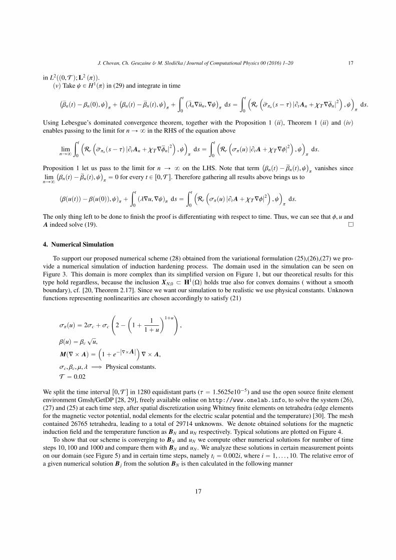
To support our proposed numerical scheme (28) obtained from the variational formulation (25),(26),(27) we pro-vide a numerical simulation of induction hardening process. The domain used in the simulation can be seen onFigure 3. This domain is more complex than its simplified version on Figure 1, but our theoretical results for thistype hold regardless, because the inclusion XN,0 Ä H1p⌦q holds true also for convex domains ( without a smoothboundary), cf. [20, Theorem 2.17]. Since we want our simulation to be realistic we use physical constants. Unknownfunctions representing nonlinearities are chosen accordingly to satisfy (21)

�⇡puq “ 2�c ` �c

˜

2 ´ˆ

1 ` 11 ` u

˙1`u¸

,

�puq “ �c?

u,

Mprˆ Aq “´

1 ` e´|rˆA|¯rˆ A,

�c, �c, µ, � ùñ Physical constants.T “ 0.02

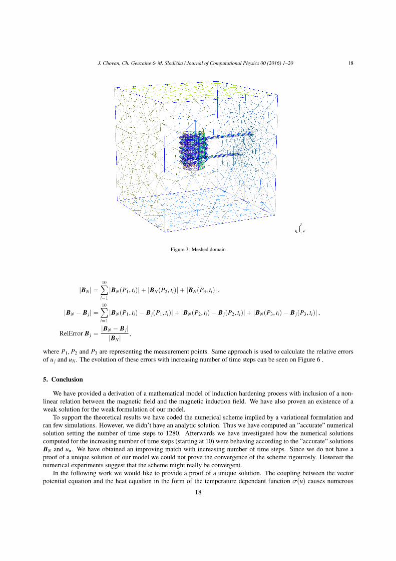
We split the time interval r0,T s in 1280 equidistant parts (⌧ “ 1.5625e10´5) and use the open source finite elementenvironment Gmsh/GetDP [28, 29], freely available online on http://www.onelab.info, to solve the system (26),(27) and (25) at each time step, after spatial discretization using Whitney finite elements on tetrahedra (edge elementsfor the magnetic vector potential, nodal elements for the electric scalar potential and the temperature) [30]. The meshcontained 26765 tetrahedra, leading to a total of 29714 unknowns. We denote obtained solutions for the magneticinduction field and the temperature function as BN and uN respectively. Typical solutions are plotted on Figure 4.

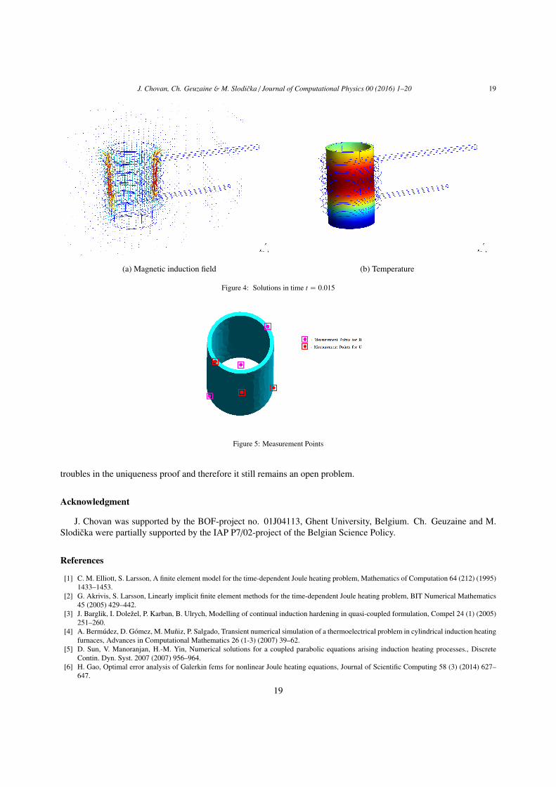
To show that our scheme is converging to BN and uN we compute other numerical solutions for number of timesteps 10, 100 and 1000 and compare them with BN and uN . We analyze these solutions in certain measurement pointson our domain (see Figure 5) and in certain time steps, namely ti “ 0.002i, where i “ 1, . . . , 10. The relative error ofa given numerical solution B j from the solution BN is then calculated in the following manner

17


Figure 3: Meshed domain

|BN | “10ÿ

i“1

|BNpP1, tiq| ` |BNpP2, tiq| ` |BNpP3, tiq| ,

|BN ´ B j| “10ÿ

i“1

|BNpP1, tiq ´ B jpP1, tiq| ` |BNpP2, tiq ´ B jpP2, tiq| ` |BNpP3, tiq ´ B jpP3, tiq| ,

RelError B j “ |BN ´ B j||BN | ,

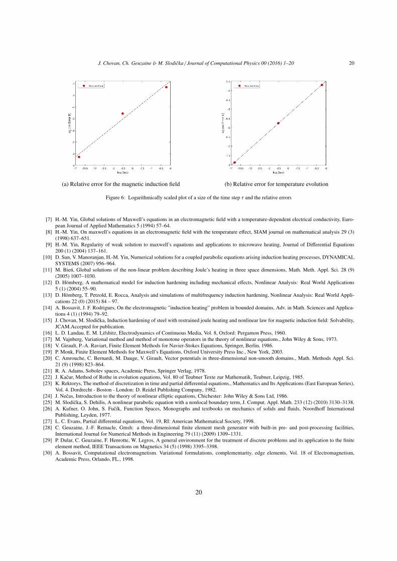
where P1, P2 and P3 are representing the measurement points. Same approach is used to calculate the relative errorsof u j and uN . The evolution of these errors with increasing number of time steps can be seen on Figure 6 .

5. Conclusion

We have provided a derivation of a mathematical model of induction hardening process with inclusion of a non-linear relation between the magnetic field and the magnetic induction field. We have also proven an existence of aweak solution for the weak formulation of our model.

To support the theoretical results we have coded the numerical scheme implied by a variational formulation andran few simulations. However, we didn’t have an analytic solution. Thus we have computed an ”accurate” numericalsolution setting the number of time steps to 1280. Afterwards we have investigated how the numerical solutionscomputed for the increasing number of time steps (starting at 10) were behaving according to the ”accurate” solutionsBN and un. We have obtained an improving match with increasing number of time steps. Since we do not have aproof of a unique solution of our model we could not prove the convergence of the scheme rigourosly. However thenumerical experiments suggest that the scheme might really be convergent.

In the following work we would like to provide a proof of a unique solution. The coupling between the vectorpotential equation and the heat equation in the form of the temperature dependant function �puq causes numerous

18


(a) Magnetic induction field (b) Temperature

Figure 4: Solutions in time t “ 0.015

Figure 5: Measurement Points

troubles in the uniqueness proof and therefore it still remains an open problem.

Acknowledgment

J. Chovan was supported by the BOF-project no. 01J04113, Ghent University, Belgium. Ch. Geuzaine and M.Slodicka were partially supported by the IAP P7/02-project of the Belgian Science Policy.

References

[1] C. M. Elliott, S. Larsson, A finite element model for the time-dependent Joule heating problem, Mathematics of Computation 64 (212) (1995)1433–1453.

[2] G. Akrivis, S. Larsson, Linearly implicit finite element methods for the time-dependent Joule heating problem, BIT Numerical Mathematics45 (2005) 429–442.

[3] J. Barglik, I. Dolezel, P. Karban, B. Ulrych, Modelling of continual induction hardening in quasi-coupled formulation, Compel 24 (1) (2005)251–260.

[4] A. Bermudez, D. Gomez, M. Muniz, P. Salgado, Transient numerical simulation of a thermoelectrical problem in cylindrical induction heatingfurnaces, Advances in Computational Mathematics 26 (1-3) (2007) 39–62.

[5] D. Sun, V. Manoranjan, H.-M. Yin, Numerical solutions for a coupled parabolic equations arising induction heating processes., DiscreteContin. Dyn. Syst. 2007 (2007) 956–964.

[6] H. Gao, Optimal error analysis of Galerkin fems for nonlinear Joule heating equations, Journal of Scientific Computing 58 (3) (2014) 627–647.

19


(a) Relative error for the magnetic induction field (b) Relative error for temperature evolution

Figure 6: Logarithmically scaled plot of a size of the time step ⌧ and the relative errors

[7] H.-M. Yin, Global solutions of Maxwell’s equations in an electromagnetic field with a temperature-dependent electrical conductivity, Euro-pean Journal of Applied Mathematics 5 (1994) 57–64.

[8] H.-M. Yin, On maxwell’s equations in an electromagnetic field with the temperature e↵ect, SIAM journal on mathematical analysis 29 (3)(1998) 637–651.

[9] H.-M. Yin, Regularity of weak solution to maxwell’s equations and applications to microwave heating, Journal of Di↵erential Equations200 (1) (2004) 137–161.

[10] D. Sun, V. Manoranjan, H.-M. Yin, Numerical solutions for a coupled parabolic equations arising induction heating processes, DYNAMICALSYSTEMS (2007) 956–964.

[11] M. Bien, Global solutions of the non-linear problem describing Joule’s heating in three space dimensions, Math. Meth. Appl. Sci. 28 (9)(2005) 1007–1030.

[12] D. Homberg, A mathematical model for induction hardening including mechanical e↵ects, Nonlinear Analysis: Real World Applications5 (1) (2004) 55–90.

[13] D. Homberg, T. Petzold, E. Rocca, Analysis and simulations of multifrequency induction hardening, Nonlinear Analysis: Real World Appli-cations 22 (0) (2015) 84 – 97.

[14] A. Bossavit, J. F. Rodrigues, On the electromagnetic ”induction heating” problem in bounded domains, Adv. in Math. Sciences and Applica-tions 4 (1) (1994) 79–92.

[15] J. Chovan, M. Slodicka, Induction hardening of steel with restrained joule heating and nonlinear law for magnetic induction field: Solvability,JCAM.Accepted for publication.

[16] L. D. Landau, E. M. Lifshitz, Electrodynamics of Continuous Media, Vol. 8, Oxford: Pergamon Press, 1960.[17] M. Vajnberg, Variational method and method of monotone operators in the theory of nonlinear equations., John Wiley & Sons, 1973.[18] V. Girault, P.-A. Raviart, Finite Element Methods for Navier-Stokes Equations, Springer, Berlin, 1986.[19] P. Monk, Finite Element Methods for Maxwell’s Equations, Oxford University Press Inc., New York, 2003.[20] C. Amrouche, C. Bernardi, M. Dauge, V. Girault, Vector potentials in three-dimensional non-smooth domains., Math. Methods Appl. Sci.

21 (9) (1998) 823–864.[21] R. A. Adams, Sobolev spaces, Academic Press, Springer Verlag, 1978.[22] J. Kacur, Method of Rothe in evolution equations, Vol. 80 of Teubner Texte zur Mathematik, Teubner, Leipzig, 1985.[23] K. Rektorys, The method of discretization in time and partial di↵erential equations., Mathematics and Its Applications (East European Series),

Vol. 4. Dordrecht - Boston - London: D. Reidel Publishing Company, 1982.[24] J. Necas, Introduction to the theory of nonlinear elliptic equations, Chichester: John Wiley & Sons Ltd, 1986.[25] M. Slodicka, S. Dehilis, A nonlinear parabolic equation with a nonlocal boundary term, J. Comput. Appl. Math. 233 (12) (2010) 3130–3138.[26] A. Kufner, O. John, S. Fucık, Function Spaces, Monographs and textbooks on mechanics of solids and fluids, Noordho↵ International

Publishing, Leyden, 1977.[27] L. C. Evans, Partial di↵erential equations, Vol. 19, RI: American Mathematical Society, 1998.[28] C. Geuzaine, J.-F. Remacle, Gmsh: a three-dimensional finite element mesh generator with built-in pre- and post-processing facilities,

International Journal for Numerical Methods in Engineering 79 (11) (2009) 1309–1331.[29] P. Dular, C. Geuzaine, F. Henrotte, W. Legros, A general environment for the treatment of discrete problems and its application to the finite

element method, IEEE Transactions on Magnetics 34 (5) (1998) 3395–3398.[30] A. Bossavit, Computational electromagnetism. Variational formulations, complementarity, edge elements, Vol. 18 of Electromagnetism,

Academic Press, Orlando, FL., 1998.

20

Documents

A formulation of a mathematical model for the induction ...geuzaine/preprints/preprint_aphi_nonlin.pdf · Journal of Computational Physics 00 (2016) 1–20 A- formulation of a mathematical