Embed Size (px)
Citation preview

HAL Id: hal-01232365https://hal.archives-ouvertes.fr/hal-01232365
Submitted on 23 Nov 2015
HAL is a multi-disciplinary open accessarchive for the deposit and dissemination of sci-entific research documents, whether they are pub-lished or not. The documents may come fromteaching and research institutions in France orabroad, or from public or private research centers.
L’archive ouverte pluridisciplinaire HAL, estdestinée au dépôt et à la diffusion de documentsscientifiques de niveau recherche, publiés ou non,émanant des établissements d’enseignement et derecherche français ou étrangers, des laboratoirespublics ou privés.
Copyright
A Formally Verified Hybrid System for Safe Advisoriesin the Next-Generation Airborne Collision Avoidance
SystemJean-Baptiste Jeannin, Khalil Ghorbal, Yanni Kouskoulas, Aurora Schmidt,
Ryan Gardner, Stefan Mitsch, André Platzer
To cite this version:Jean-Baptiste Jeannin, Khalil Ghorbal, Yanni Kouskoulas, Aurora Schmidt, Ryan Gardner, et al..A Formally Verified Hybrid System for Safe Advisories in the Next-Generation Airborne CollisionAvoidance System. International Journal on Software Tools for Technology Transfer, Springer Verlag,2017, 19 (6), pp.717-741. �10.1007/s10009-016-0434-1�. �hal-01232365�

Noname manuscript No.(will be inserted by the editor)
A Formally Verified Hybrid System for Safe Advisoriesin the Next-Generation Airborne Collision Avoidance System
Jean-Baptiste Jeannin · Khalil Ghorbal · Yanni Kouskoulas · Aurora Schmidt ·Ryan Gardner · Stefan Mitsch · Andre Platzer
the date of receipt and acceptance should be inserted later
Abstract The Next-Generation Airborne Collision Avoid-ance System (ACAS X) is intended to be installed on alllarge aircraft to give advice to pilots and prevent mid-aircollisions with other aircraft. It is currently being developedby the Federal Aviation Administration (FAA). In this pa-per we determine the geometric configurations under whichthe advice given by ACAS X is safe under a precise set ofassumptions and formally verify these configurations usinghybrid systems theorem proving techniques. We considersubsequent advisories and show how to adapt our formalverification to take them into account. We examine the cur-rent version of the real ACAS X system and discuss somecases where our safety theorem conflicts with the actual ad-visory given by that version, demonstrating how formal, hy-brid systems proving approaches are helping ensure the safetyof ACAS X. Our approach is general and could also be usedto identify unsafe advice issued by other collision avoidancesystems or confirm their safety.
Jean-Baptiste Jeannin∗
Samsung Research America, Mountain View, CA, USA
Khalil Ghorbal∗
Inria, France
Yanni KouskoulasThe Johns Hopkins University Applied Physics Laboratory, USA
Aurora SchmidtThe Johns Hopkins University Applied Physics Laboratory, USA
Ryan GardnerThe Johns Hopkins University Applied Physics Laboratory, USA
Stefan Mitsch∗
Johannes Kepler University, Linz, Austria
Andre PlatzerCarnegie Mellon University, Pittsburgh, PA, USA∗ This work was performed at Carnegie Mellon University
1 Introduction
With growing air traffic, the airspace becomes more crowded,and the risk of airborne collisions between aircraft increases.In the 1970s, after a series of mid-air collisions, the FederalAviation Administration (FAA) decided to develop an on-board collision avoidance system: the Traffic Alert and Col-lision Avoidance System (TCAS). This program had greatsuccess, and prevented many mid-air collisions over the years.Some accidents still happened; for example, a collision overUberlingen in 2002 occurred due to conflicting advice be-tween TCAS and air traffic control. Airspace managementwill evolve significantly over the next decade with the intro-duction of the next-generation air traffic management sys-tem; this will create new requirements for collision avoid-ance. To meet these new requirements, the FAA has decidedto develop a new system: the Next-Generation Airborne Col-lision Avoidance System, known as ACAS X [4,11,15].
Like TCAS, ACAS X avoids collisions by giving ver-tical guidance to an aircraft’s pilot. A typical scenario in-volves two aircraft: the ownship where ACAS X is installed,and another aircraft called the intruder that is at risk of col-liding with the ownship. ACAS X is designed to avoid NearMid-Air Collisions (NMACs), situations where two aircraftcome within rp = 500 ft horizontally and hp = 100 ft ver-tically [15] of each other. The NMAC definition describes avolume centered around the ownship, shaped like a hockeypuck of radius rp and half-height hp.
In order to be accepted by pilots, and thus operationallysuitable, ACAS X needs to strike a balance between givingadvice that helps pilots avoid collisions but also minimizinginterruptions. These goals drive the design in opposite di-rections each other, and cannot both be perfectly met in thepresence of unknown pilot behavior. As part of the ACAS Xdevelopment process, this work focuses on precisely charac-terizing the circumstances in which ACAS X gives safe ad-
2 J.-B. Jeannin, K. Ghorbal, Y. Kouskoulas, A. Schmidt, R. Gardner, S. Mitsch and A. Platzer
Table 1 ACAS X advisories and their modeling variables
ACAS X Specification [13] Our modelVertical Rate Range Strength Delay Sign Advisory
Advisory Description Min (ft/min) Max (ft/min) alo δ (s) w vlo (ft/min)DNC2000 Do Not Climb at more than 2,000 ft/min −∞ +2000 g/4 5 −1 +2000DND2000 Do Not Descend at more than 2,000 ft/min −2000 +∞ g/4 5 +1 −2000DNC1000 Do Not Climb at more than 1,000 ft/min −∞ +1000 g/4 5 −1 +1000DND1000 Do Not Descend at more than 1,000 ft/min −1000 +∞ g/4 5 +1 −1000DNC500 Do Not Climb at more than 500 ft/min −∞ +500 g/4 5 −1 +500DND500 Do Not Descend at more than 500 ft/min −500 +∞ g/4 5 +1 −500DNC Do Not Climb −∞ 0 g/4 5 −1 0DND Do Not Descend 0 +∞ g/4 5 +1 0MDES Maintain at least current Descent rate −∞ current g/4 5 −1 currentMCL Maintain at least current Climb rate current +∞ g/4 5 +1 currentDES1500 Descend at at least 1,500 ft/min −∞ −1500 g/4 5 −1 −1500CL1500 Climb at at least 1,500 ft/min +1500 +∞ g/4 5 +1 +1500
SDES1500 Strengthen Descent to at least 1,500 ft/min −∞ −1500 g/3 3 −1 −1500SCL1500 Strengthen Climb to at least 1,500 ft/min +1500 +∞ g/3 3 +1 +1500SDES2500 Strengthen Descent to at least 2,500 ft/min −∞ −2500 g/3 3 −1 −2500SCL2500 Strengthen Climb to at least 2,500 ft/min +2500 +∞ g/3 3 +1 +2500
COC Clear of Conflict −∞ +∞ Not applicableMTLO Multi-Threat Level-Off Not applicable
vice, and where safety is traded off for operational suitabil-ity, helping to identify modifications that improve its safetyand performance.
1.1 Airborne Collision Avoidance System ACAS X
In order to prevent an NMAC with other aircraft, ACAS Xuses various sensors to determine the position of the own-ship, as well as the positions of any intruders [5]. It com-putes its estimate of the best pilot action by linearly interpo-lating a precomputed table of scores for actions, and, if ap-propriate, issuing an advisory to avoid potential collisions [6]through a visual display and a voice message.
An advisory is a request to the pilot of the ownship to al-ter or maintain her vertical speed. ACAS X advisories arestrictly vertical, and never request any horizontal maneu-vering. Table 1 shows the advisories ACAS X can issue.For example, Do-Not-Climb (DNC) requests that the pilotnot climb, and Climb-1500 (CL1500) requests that the pi-lot climb at more than 1500 ft/min. The current version ofACAS X can issue a total of 16 different advisories plusClear-of-Conflict (COC), which indicates that no action isnecessary, and Multi-Threat-Level-Off (MTLO), which isused in the case of multiple intruders. To comply with an ad-visory, the pilot must adjust her vertical rate to fall within theadvised vertical rate range. Based on previous research [13],the pilot is assumed to do so using a vertical acceleration ofstrength at least alo starting after a delay of at most δ afterthe advisory has been announced by ACAS X.
At the heart of ACAS X is a table whose domain de-scribes the instantaneous state of an encounter, and whoserange is a set of scores for each possible action [13,16]. The
table is obtained from a Markov Decision Process (MDP)approximating the dynamics of the system in a discretiza-tion of the state-space, and optimized using dynamic pro-gramming to maximize the expected value of events overall future paths for each action [13]. Near Mid-Air Colli-sion events, for example, are associated with large negativevalues and issuing an advisory is associated with a smallnegative value. The policy is to choose the action with thehighest expected value from a multilinear interpolation ofgrid points in this table. ACAS X uses this table, along withsome heuristics, to determine the best action to take for thegeometry and dynamic conditions in which it finds itself.
1.2 Identifying Formally Verified Safe Regions
Since ACAS X involves both discrete advisories to the pi-lot and continuous dynamics of aircraft, it is natural to for-mally verify it using hybrid systems. However the complex-ity of ACAS X, which uses at its core a large lookup table—defining 29,212,664 interpolation regions within a 5-dimensionalstate-space—makes the direct use of hybrid systems verifi-cation techniques intractable. Our approach is different. Itidentifies safe regions in the state space of the system wherewe prove formally that the current positions and velocitiesof the aircraft ensure that a particular advisory, if followed,prevents all possible NMACs. Then it compares these re-gions to the configurations where the ACAS X table returnsthis same advisory. Moreover our safe regions are symbolicin their parameters, and can thus be easily adapted to newparameters or new versions of ACAS X.
Going beyond the results of [12], this paper devises andformally proves safety regions for advisories that can be cor-

A Formally Verified Hybrid System for Safe Advisories in the Next-Generation Airborne Collision Avoidance System 3
rected later on. In that context, an advisory need not be safeon its own to be considered acceptable, but the system needsto be able to correct it with a subsequent advisory. This isparticularly useful to assess the safety of preventative ad-visories, and leads to the discovery of very relevant unex-pected behaviors of the system.
Our results provide independent characterizations of theACAS X behavior to provide a clear and complete pictureof its performance. Our method can be used by the ACAS Xdevelopment team in two ways. It provides a mathemati-cal proof—with respect to a hybrid systems model—thatACAS X is absolutely safe for some configurations of theaircraft. Additionally, when ACAS X is not safe, it is able toidentify unsafe or unexpected behaviors and suggests waysof correcting them.
Our approach of formally deriving safe regions then com-paring them to the behavior of an industrial system is, as faras we are aware, the first of its kind in the formal verifica-tion of hybrid systems. The approach may be valuable forverifying or assessing properties of other systems with sim-ilar complexities, or also using large lookup tables, which isa common challenge in practice. Finally, the constraints weidentified for safety are fairly general and could be used toanalyze other collision avoidance systems.
The paper is organized as follows. After an overview ofthe method in Sect. 2, we start with a simple two-dimensionalmodel assuming immediate reaction of the pilot in Sect. 3.We extend the model to account for the reaction time of thepilot in Sect. 4, consider more liberal safe regions to toler-ate advisories that are only safe if followed up by suitablesubsequent advisories in Sect. 5, and extend the results toa three-dimensional model in Sect. 6. Relationships and ex-tensions are discussed in Sect. 7. In Sect. 8, we compare theadvisory recommended by a core component of ACAS Xwith our safe regions, identifying the circumstances wheresafety of those ACAS X advisories is guaranteed within ourmodel.
2 Overview of the ACAS X Modelling Approach
To construct a safe region of an advisory for an aircraft,imagine following all allowable trajectories of the ownshiprelative to the intruder, accounting for every possible posi-tion of the ownship and its surrounding puck at every futuremoment in time. The union of all such positions of the puckdescribes a potentially unsafe region; for each point thereexists a trajectory that results in an NMAC. Dually, if theintruder is outside this set, i.e., in the safe region, an NMACcannot occur in the model.
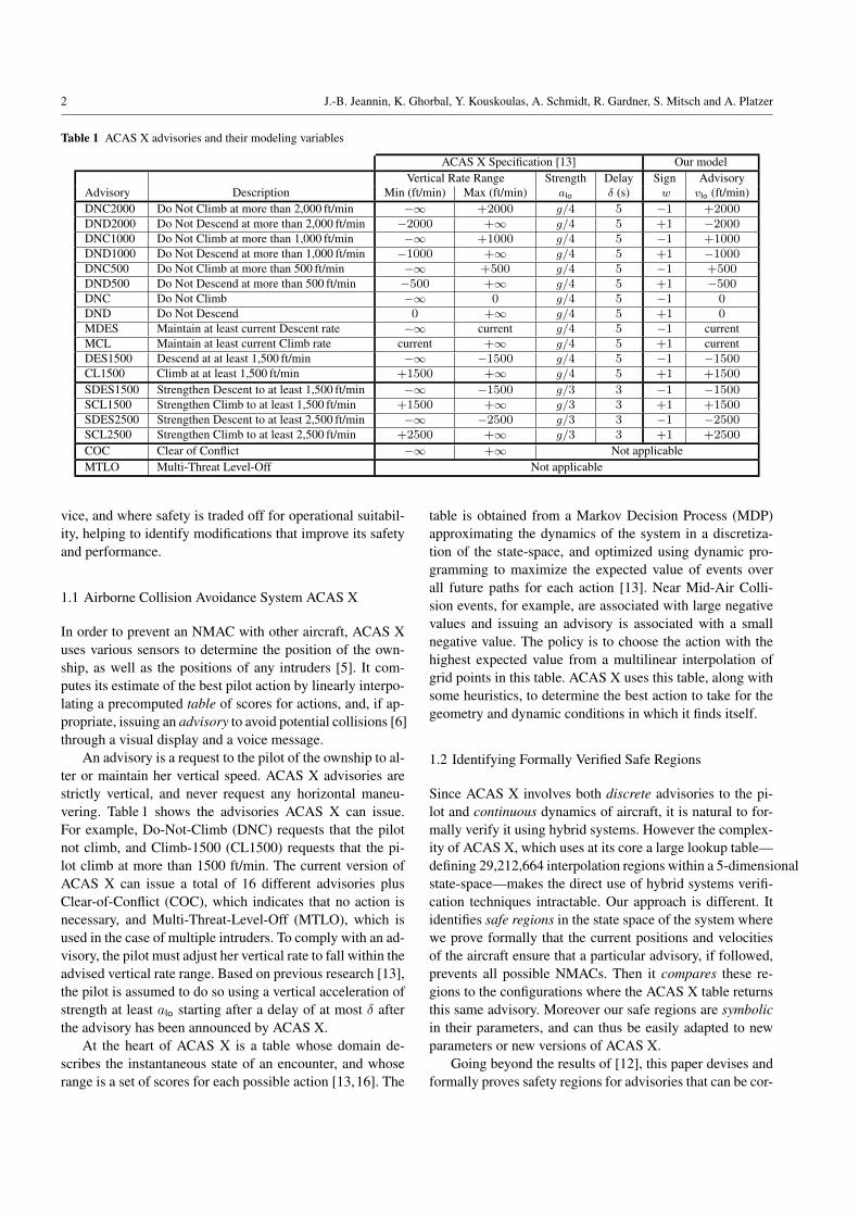
Fig. 1 depicts an example of a head-on encounter and itsassociated safe region for the advisory CL1500, projected ina vertical plane with both aircraft. It is plotted in a coordi-nate system fixed to the intruder and centered at the initial
O
I
rvrp
r
O
Iv vI
rp
hp
θv
M
(a) Top view of the encounter
O
I
rvrp
r
O
Iv vI
rp
hp
θv
M
(b) Side view of the encounter
Fig. 2 An encounter between ownship O and intruder I, with NMACpuck in gray of horizontal radius rp and vertical radius hp
position of the ownship. The ownship, surrounded by thepuck, starts at position 1 and traces out a trajectory follow-ing the red curve. It first accelerates vertically with g/4 untilreaching the desired vertical velocity of +1500 ft/min at po-sition 3. It then climbs at +1500 ft/min, respecting the spec-ification of Table 1. The green safe-region indicates startingpoints in the state space for which the aircraft will remainsafe for the duration of the encounter when following theCL1500 advisory. Note that no safe region exists above thetrajectory since the ownship could accelerate vertically atgreater than g/4 or climb more than +1500 ft/min, in accor-dance with Table 1.
2.1 Model of Dynamics
Let us consider an encounter between two planes—ownshipOand intruder I , as portrayed in Fig. 2. Following the notationof the ACAS X community [13], let r = ‖r‖ be the hori-zontal distance between the aircraft (called range) and h theheight of the intruder relative to the ownship. We assumethat the relative horizontal velocity rv of the intruder withrespect to the ownship is constant throughout the encounter.I.e., from a top view, the planes follow straight-line trajec-tories. Let θv be the non-directed angle between rv and theline segment r. In the vertical dimension, we assume thatthe ownship’s vertical velocity v can vary at any moment,while the intruder’s vertical velocity vI is fixed throughoutthe encounter. Moreover, we assume that the magnitude ofthe vertical acceleration of the ownship cannot exceed ad inabsolute value.
Our analysis considers all these as symbolic parame-ters and is, thus, valid for any value they might have. Fora typical encounter, r varies between 0 nmi and 7 nmi,1 hbetween −4,000 ft and 4,000 ft, rv = ‖rv‖ between 0 kts
1 We use units most common in the aerospace community, eventhough they are not part of the international system, including nauti-
4 J.-B. Jeannin, K. Ghorbal, Y. Kouskoulas, A. Schmidt, R. Gardner, S. Mitsch and A. Platzer
Fig. 1 Nominal trajectory of the ownship (red) and safe region for the intruder (green), immediate response
and 1,000 kts, and v and vI between −5,000 ft/min and+5,000 ft/min. The acceleration ad is usually g/2, whereg is Earth’s gravitational acceleration. The NMAC puck ofACAS X has radius rp = 500 ft and half-height hp = 100 ft.
2.2 Model of Advisories
Recall that ACAS X prevents NMACs by giving advisoriesto the ownship’s pilot. Every advisory, except Clear-of-Conflict(COC), has a vertical rate range of the form (−∞, vlo] or[vlo,+∞) for some vertical rate vlo (Table 1), which we callthe target vertical velocity. We model any advisory by itscorresponding target vertical velocity vlo, and a binary vari-able w for its orientation, whose value is −1 if the verti-cal rate range of the advisory is (−∞, vlo] and +1 if it is[vlo,+∞). This symbolic encoding can represent many ad-visories and is robust to changes in the ACAS X advisoryset. As a matter of fact, the only advisory that this symbolicencoding cannot handle is the recently-added Multi-ThreatLevel-Off (MTLO) advisory, only relevant in the presenceof multiple intruders.
Following the ACAS X design [13], we assume that theownship pilot complies with each advisory within δ seconds,and that she accelerates with acceleration at least alo to reachthe target vertical velocity.
3 Safe Region for an Immediate Pilot Response
We present in this section a simplified version of the dynam-ics from Sect. 2.1. We give a hybrid model for this simplifiedsystem and prove its safety. The new assumptions will be re-laxed in later sections to achieve the safety verification of thefull model of Sect. 2.1.
cal miles nmi (1,852metres), knots kts (nautical miles per hour), feetft (0.3048meter) and minutes min (60 seconds).
3.1 Model
In this section, we assume that the ownship and intruder areflying head-on (θv = 180◦). We also assume that the pi-lot reacts immediately to any advisory (δ = 0 s), and thatthe advisory COC is not allowed. These assumptions will berelaxed in Sect. 4 and Sect. 6. The model in this section per-mits updates to the resolution advisory but, unlike in Sect. 5,each advisory issued has to be safe, i.e., it has to prevent anyNMAC at any future time, even if followed forever. We as-sume that r is a scalar: if r ≥ 0 then the ownship is flyingtowards the intruder, otherwise it is flying away from it. Bothcases could require an advisory. Since the ownship and in-truder are flying head-on with straight line trajectories, thereexists a vertical plane containing both their trajectories. Inthis plane, the puck becomes a rectangle centered aroundthe ownship, of width 2rp and height 2hp, and there is anNMAC if and only if the intruder is in this rectangle (in grayon Fig. 1).
3.2 Differential Dynamic Logic and KeYmaera X
We model our system using Differential Dynamic Logic dL [19,20,21,22], a logic for reasoning about hybrid programs, aprogramming language for hybrid systems. The logic dLallows discrete assignments, control structures, and execu-tion of differential equations. It is implemented in the theo-rem prover KeYmaera X [8], that we use to verify our saferegions with respect to our models. All the KeYmaera Xmodels and proofs of this paper can be found at http://www.ls.cs.cmu.edu/pub/AcasX-long.zip.
The dL formula for the model that we use in this sectionis given in Eq. (1). We use the notation L−1impl for the saferegion: the letter L stands for lower bound (for w = 1; itis an upper bound for w = −1); the subscript impl standsfor implicit safe region, as described in Sect. 3.3; and the su-perscript −1 indicates that the region is safe for unboundedtime; the rationale behind its use will become more clear in

A Formally Verified Hybrid System for Safe Advisories in the Next-Generation Airborne Collision Avoidance System 5
Sect. 5.2.
1 rp ≥ 0 ∧ hp > 0 ∧ rv ≥ 0 ∧ alo > 0∧2 (w = −1 ∨ w = 1) ∧ L−1impl(r, h, v, w, vlo)→3 [( ( ?true ∪4 (w := −1 ∪ w := 1); vlo := ∗;5 ?L−1impl(r, h, v, w, vlo); advisory := (w, vlo) );
6 a := ∗;7 {r′ = −rv, h′ = −v, v′ = a & wv ≥ wvlo ∨ wa ≥ alo}8 )∗] (|r| > rp ∨ |h| > hp)
(1)
This formula of the form p → [α]q says all executions ofhybrid program α starting in a state satisfying logical for-mula p end up in a state satisfying q. It is akin to the Hoaretriple {p}α{q}with precondition p and postcondition q. Theprecondition in Eq. (1) imposes constraints on several con-stants, as well as the formula L−1impl(r, h, v, w, vlo) (whichwe identify below) that forces the intruder to be in a saferegion for an initial advisory (w, vlo). We cannot guaran-tee safety if the intruder starts initially in an unsafe region.The postcondition encodes absence of NMAC. Lines 3–5express the action of the ACAS X system. The nondeter-ministic choice operator ∪ in Line 3 expresses that the sys-tem can either continue with the same advisory by doingnothing—just testing the trivial condition ?true—this en-sures it always has a valid choice and cannot get stuck. Oth-erwise it can choose a new advisory (w, vlo) in Line 4 thatpasses the safety condition L−1impl(r, h, v, w, vlo) in Line 5—advisory represents the next message to the pilot. Line 6 ex-presses the action of the ownship pilot, who can nondeter-ministically choose an arbitrary acceleration (a := ∗). Theownship and intruder aircraft then follow the continuous dy-namics in Line 7. The evolution of the variables r, h and vis expressed by a differential equation, and requires (usingthe operator &) that the ownship evolves towards its targetvertical velocity vlo at acceleration alo (condition wa ≥ alo),unless it has already reached vertical velocity vlo (conditionwv ≥ wvlo). Finally, the star ∗ on Line 8 indicates that theprogram can be repeated any number of times, allowing thesystem to go through several advisories.
3.3 Implicit Formulation of the Safe Region
In this section, we identify what formula can be used as saferegion L−1impl(r, h, v, w, vlo) to prove Eq. (1). As in Sect. 2,we use a coordinate system fixed to the intruder and with itsorigin at the initial position of the ownship (see Fig. 1).
First case: if w = +1 and vlo ≥ v. Fig. 1 shows, in red, apossible trajectory of an ownship following exactly the re-quirements of ACAS X. This nominal trajectory of the own-ship is denoted by N and merely represents one possible
scenario to consider. The pilot reacts immediately, and theownship starts accelerating vertically with acceleration alountil reaching the target vertical velocity vlo—describing aparabola—then climbs at vertical velocity vlo along a straightline. Horizontally, the relative velocity rv remains constant.Integrating the differential equations in Eq. (1) Line 7, theownship position (rn, hn) at time t along N is given by:
(rn, hn) =
(rvt ,
alo2t2 + vt
)if 0 ≤ t < vlo − v
alo(a)(
rvt , vlot−(vlo − v)2
2ar
)ifvlo − valo
≤ t (b)
(2)
Recall that in the ACAS X specification, the ownshipmoves vertically with acceleration of at least alo, then con-tinues with vertical velocity of at least vlo. Therefore allpossible future positions of the ownship will turn out to beabove the red nominal trajectory. An intruder is safe if itsposition is always either to the side of or under any puckcentered on a point in N , that is:
∀t.∀rn.∀hn.((rn, hn) ∈ N → |r−rn| > rp∨h−hn < −hp
)(3)
We call this formulation the implicit formulation of the saferegion. It does not give explicit equations for the safe regionborder, but expresses them instead implicitly by quantifierswith respect to the nominal trajectory from Eq. (2).
Generalization. The reasoning above is generalized to thecase where the target vertical velocity is exceeded (vlo <
v) —which happens after the parabola part of the nominaltrajectory— and symmetrically to the case of descend-typeadvisories (w = −1).
Eq. (1) gives the pilot ample flexibility in how to respondto a resolution advisory and gives ACAS X full flexibil-ity to choose any advisories respecting L−1impl(r, h, v, w, vlo).In particular, we cannot assume the pilot would follow thenominal trajectory N . We prove that, nevertheless, the saferegions identified like this respect safety property Eq. (1).The implicit formulation of the safe region isL−1impl(r, h, v, w, vlo)
in Fig. 3, and verified to be safe in KeYmaera X:
Theorem 1 (Correctness of implicit safe regions) The dLformula given in Eq. (1) is valid. That is as long as the advi-sories followed obey formula L−1impl there will be no NMAC.
3.4 Explicit Formulation of the Safe Region
The implicit formulation of the safe region gives an intuitiveunderstanding of where it is safe for the intruder to be. How-ever, because it still contains quantifiers, its use comes at theextra cost of eliminating the quantifiers, which is inefficient

6 J.-B. Jeannin, K. Ghorbal, Y. Kouskoulas, A. Schmidt, R. Gardner, S. Mitsch and A. Platzer
Implicit formulation
A(t, hn, v, w, vlo) ≡
(0 ≤ t <
max(0, w(vlo − v))alo
∧ hn =walo
2t2 + vt
)
∨
(t ≥
max(0, w(vlo − v))alo
∧ hn = vlot−wmax(0, w(vlo − v))2
2alo
)L−1impl(r, h, v, w, vlo) ≡ ∀t.∀rn.∀hn.
(rn = rvt ∧A(t, hn, v, w, vlo)→ (|r − rn| > rp ∨ w(h− hn) < −hp)
)Explicit formulation
case−11 (r, v, w, vlo) ≡ −rp ≤ r < −rp −
rv min(0, wv)
alocase−1
2 (r, v, w, vlo) ≡ −rp −rv min(0, wv)
alo≤ r ≤ rp −
rv min(0, wv)
alo
bound1(r, h, v, w, vlo) ≡ wrv2h <alo
2(r + rp)
2 + wrvv(r + rp)− rv2hp bound2(r, h, v, w, vlo) ≡ wh < −min(0, wv)2
2alo− hp
case−13 (r, v, w, vlo) ≡ rp −
rv min(0, wv)
alo< r ≤ rp +
rv max(0, w(vlo − v))alo
case−14 (r, v, w, vlo) ≡ rp +
rv max(0, w(vlo − v))alo
< r
bound3(r, h, v, w, vlo) ≡ wrv2h <alo
2(r − rp)2 + wrvv(r − rp)− rv2hp
bound4(r, h, v, w, vlo) ≡ (rv = 0) ∨(wrvh < wvlo(r − rp)−
rv max(0, w(vlo − v))2
2alo− rvhp
)case−1
5 (r, v, w, vlo) ≡ −rp ≤ r < −rp +rv max(0, w(vlo − v))
alocase−1
6 (r, v, w, vlo) ≡ −rp +rv max(0, w(vlo − v))
alo≤ r
bound5(r, h, v, w, vlo) ≡ wrv2h <alo
2(r + rp)
2 + wrvv(r + rp)− rv2hp
bound6(r, h, v, w, vlo) ≡ (rv = 0 ∧ r > rp) ∨(wrvh < wvlo(r + rp)−
rv max(0, w(vlo − v))2
2alo− rvhp
)L−1expl(r, h, v, w, vlo) ≡
(wvlo ≥ 0→
4∧i=1
(case−1i (r, v, w, vlo)→ boundi(r, h, v, w, vlo))
)
∧(wvlo < 0→
6∧i=5
(case−1i (r, v, w, vlo)→ boundi(r, h, v, w, vlo))
)
Fig. 3 Implicit and explicit formulations of the safe region for an immediate response (lower bounds for w = 1, upper bound for w = −1)
and impractical to repeatedly compute during the compar-ison part of our analysis. An efficient comparison with theACAS X table, as described in Sect. 8, can only be achievedwith a quantifier-free, explicit formulation, that we presentin this section. We show that both formulations are equiva-lent. As for the implicit formulation, we derive the equationsfor one representative case before generalizing them.
First case: ifw = +1, rv > 0, v < 0 and vlo ≥ 0. We are inthe case shown in Fig. 1 and described in detail in Sect. 3.3.The nominal trajectoryN is given by Eq. (2). The boundaryof the (green) safe region in Fig. 1 is drawn by either thebottom left hand corner, the bottom side or the bottom righthand corner of the puck. For this case, this boundary canbe characterized by a set of equations (where cases 1 to 4follow cases 1 to 4 of Fig. 3):
0. positions left of the puck’s initial position (r < −rp) arein the safe region;
1. then the boundary follows the bottom left hand corner ofthe puck as it is going down the parabola of Eq. (2)(a);therefore for −rp ≤ r < −rp − rvv
alo, the position (r, h)
is safe if and only if h < alo
2rv2 (r+rp)2+ v
rv(r+rp)−hp;
2. following this, the boundary is along the bottom sideof the puck as it is at the bottom of the parabola ofEq. (2)(a); therefore for −rp − rvv
a ≤ r ≤ rp − rvvalo
,the position (r, h) is in the safe region if and only ifh < − v2
2alo− hp;
3. then the boundary follows the bottom right hand cornerof the puck as it is going up the parabola of Eq. (2)(a);therefore for rp− rvv
alo< r ≤ rp+ rv(vlo−v)
alo, the position
(r, h) is safe if and only if h < alo
2rv2 (r − rp)2 + vrv(r −
rp)− hp;4. finally the boundary follows the bottom right-hand cor-
ner of the puck as it is going up the straight line ofEq. (2)(b); therefore for rp + rv(vlo−v)
alo< r, the po-
sition (r, h) is in the safe region if and only if h <vlorv(r − rp)− (vlo−v)2
2ar− hp.
A Formally Verified Hybrid System for Safe Advisories in the Next-Generation Airborne Collision Avoidance System 7
Generalization. The general case is given in the formulaL−1expl(r, h, v, w, vlo) of Fig. 3. The cases 1-4 and their asso-ciated bounds are for the case wvlo ≥ 0, whereas cases 5and 6 and associated bounds are for wvlo < 0; both cases 5and 6 follow the bottom left-hand corner of the puck as it isgoing along the nominal trajectory. We use KeYmaera X toformally prove that this explicit safe region formulation isequivalent to its implicit counterpart:
Lemma 1 (Equivalence of explicit safe regions) If w =
±1, rp ≥ 0, hp > 0, rv ≥ 0 and alo > 0, then the conditionsL−1impl(r, h, v, w, vlo) and L−1expl(r, h, v, w, vlo) are equivalent.
Since the assumptions of Lemma 1 are invariants of themodel in Eq. (1), the explicit safe regions give a model thatinherits safety from Theorem 1, which we formally provein KeYmaera X by a combination of contextual equivalencereasoning and monotonicity reasoning [22] to embed theconditional equivalence from Lemma 1 into the context ofTheorem 1.
Corollary 1 (Correctness of explicit safe regions) The dLformula given in Eq. (1) remains valid when replacing alloccurrences of L−1impl with L−1expl. That is as long as the advi-sories followed obey formula L−1expl there will be no NMAC.
4 Safe Region for a Delayed Pilot Response
Since the pilot will need some time to react to an advisoryissued by ACAS X, we generalize the model of Sect. 3 toaccount for a non-deterministic, non-zero pilot delay, andfor periods of time where the system does not issue an advi-sory (i.e., COC). In Fig. 4, for example, the pilot reacts to aCL1500 advisory only after a certain reaction delay duringwhich she was still in the process of initiating a descent.
4.1 Model
In this section, we still assume that the ownship and intruderare flying head-on (θv = 180◦). We use the same conven-tions as in Sect. 3 for r and rv . The model includes an initialperiod where there is no compliance with any advisory—the ownship accelerates non-deterministically (within lim-its) in the vertical direction. As before, we derive the saferegions by considering all possible positions of the own-ship’s puck in all possible trajectories that might evolve inthe encounter. To represent pilot delay for an advisory, themodel assumes an immediate advisory, and period of non-compliance δ, representing the time it takes the pilot to re-spond. To represent COC, the model looks for a safe advi-sory it can issue ε in the future if necessary, where ε is thesystem delay—i.e., the time before the system can issue a
new advisory—and shortest COC. Hence the period of non-compliance is ε+ δ.
1 rp ≥ 0 ∧ hp > 0 ∧ rv ≥ 0 ∧ alo > 0 ∧ ad ≥ 0 ∧ δ ≥ 0
2 ∧ ε ≥ 0 ∧ (w = −1 ∨ w = 1) ∧Ddimpl(r, h, v, w, vlo)→
3 [((?true ∪
4 (w := −1 ∪ w := 1); vlo := ∗;4 (d := δ; ?Dd
impl(r, h, v, w, vlo); adv := (w, vlo) ∪5 d := δ + ε; ?Dd
impl(r, h, v, w, vlo); adv := COC));
6 a := ∗; ?(wa ≥ −ad); t := 0;
7 {r′ = −rv, h′ = −v, v′ = a,d′ = −1, t′ = 1 &
8 (t ≤ ε) ∧ (d ≤ 0→ wv ≥ wvlo ∨ wa ≥ alo)}9 )∗] (|r| > rp ∨ |h| > hp)
(4)
We modify the model of Eq. (1) to capture these newideas, and obtain the model of Eq. (4), highlighting the dif-ferences in bold. The structure, precondition (lines 1 and2) and postcondition (line 9) are similar. The clock d, ifpositive, represents the amount of time until the ownshippilot must respond to the current advisory to remain safe.Lines 3 to 5 represent the actions of the ACAS X system.As before, the system can continue with the same advisory(?true). Otherwise it can select a safe advisory (w, vlo) to beapplied after at most delay δ; or it can safely remain silent,displaying COC, if it knows an advisory (w, vlo) that is safeif it is followed after a combined pilot and system and pi-lot delay of δ + ε. In line 6, the pilot non-deterministicallychooses an acceleration (a := ∗), within some limit (wa ≥−ad). The set of differential equations in line 7 describesthe system’s dynamics, and the conditions in line 8 use theclock t to ensure that continuous time does not evolve longerthan system delay ε without a system response (t ≤ ε).Those conditions also ensure that when d ≤ 0 the pilotstarts complying with the advisory. The model is structuredso that the pilot can safely delay responding to an advisoryfor up to δ, and the system can additionally delay issuingan advisory associated with COC for up to ε. Because ofthe loop in our model (line 9), the safety guarantees of thistheorem apply to encounters whose advisories change as theencounter evolves, encounters with periods of no advisory,and encounters where the ownship pilot exhibits some non-deterministic behavior in the vertical dimension.
In the rest of the section we use the same approach asin Sect. 3: we first derive an implicit formulation, then anequivalent explicit formulation of the safe region, and provethat the safe region guarantees that the intruder cannot causean NMAC.
4.2 Implicit Formulation of the Safe Region
As in Sect. 3.3, let us place ourselves in the coordinate sys-tem centered on the current position of the ownship and
8 J.-B. Jeannin, K. Ghorbal, Y. Kouskoulas, A. Schmidt, R. Gardner, S. Mitsch and A. Platzer
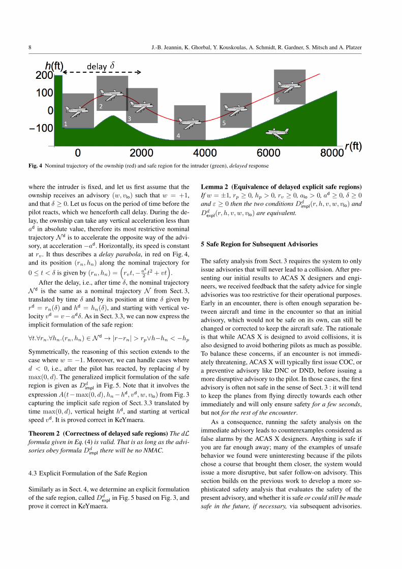
Fig. 4 Nominal trajectory of the ownship (red) and safe region for the intruder (green), delayed response
where the intruder is fixed, and let us first assume that theownship receives an advisory (w, vlo) such that w = +1,and that δ ≥ 0. Let us focus on the period of time before thepilot reacts, which we henceforth call delay. During the de-lay, the ownship can take any vertical acceleration less thanad in absolute value, therefore its most restrictive nominaltrajectory N d is to accelerate the opposite way of the advi-sory, at acceleration −ad. Horizontally, its speed is constantat rv . It thus describes a delay parabola, in red on Fig. 4,and its position (rn, hn) along the nominal trajectory for0 ≤ t < δ is given by (rn, hn) =
(rvt,−ad
2 t2 + vt
).
After the delay, i.e., after time δ, the nominal trajectoryN d is the same as a nominal trajectory N from Sect. 3,translated by time δ and by its position at time δ given byrd = rn(δ) and hd = hn(δ), and starting with vertical ve-locity vd = v−adδ. As in Sect. 3.3, we can now express theimplicit formulation of the safe region:
∀t.∀rn.∀hn.(rn, hn) ∈ N d → |r−rn| > rp∨h−hn < −hp
Symmetrically, the reasoning of this section extends to thecase where w = −1. Moreover, we can handle cases whered < 0, i.e., after the pilot has reacted, by replacing d bymax(0, d). The generalized implicit formulation of the saferegion is given as Dd
impl in Fig. 5. Note that it involves theexpression A(t−max(0, d), hn−hd, vd, w, vlo) from Fig. 3capturing the implicit safe region of Sect. 3.3 translated bytime max(0, d), vertical height hd, and starting at verticalspeed vd. It is proved correct in KeYmaera.
Theorem 2 (Correctness of delayed safe regions) The dLformula given in Eq. (4) is valid. That is as long as the advi-sories obey formula Dd
impl there will be no NMAC.
4.3 Explicit Formulation of the Safe Region
Similarly as in Sect. 4, we determine an explicit formulationof the safe region, called Dd
expl in Fig. 5 based on Fig. 3, andprove it correct in KeYmaera.
Lemma 2 (Equivalence of delayed explicit safe regions)If w = ±1, rp ≥ 0, hp > 0, rv ≥ 0, alo > 0, ad ≥ 0, δ ≥ 0
and ε ≥ 0 then the two conditions Ddimpl(r, h, v, w, vlo) and
Ddexpl(r, h, v, w, vlo) are equivalent.
5 Safe Region for Subsequent Advisories
The safety analysis from Sect. 3 requires the system to onlyissue advisories that will never lead to a collision. After pre-senting our initial results to ACAS X designers and engi-neers, we received feedback that the safety advice for singleadvisories was too restrictive for their operational purposes.Early in an encounter, there is often enough separation be-tween aircraft and time in the encounter so that an initialadvisory, which would not be safe on its own, can still bechanged or corrected to keep the aircraft safe. The rationaleis that while ACAS X is designed to avoid collisions, it isalso designed to avoid bothering pilots as much as possible.To balance these concerns, if an encounter is not immedi-ately threatening, ACAS X will typically first issue COC, ora preventive advisory like DNC or DND, before issuing amore disruptive advisory to the pilot. In those cases, the firstadvisory is often not safe in the sense of Sect. 3 : it will tendto keep the planes from flying directly towards each otherimmediately and will only ensure safety for a few seconds,but not for the rest of the encounter.
As a consequence, running the safety analysis on theimmediate advisory leads to counterexamples considered asfalse alarms by the ACAS X designers. Anything is safe ifyou are far enough away; many of the examples of unsafebehavior we found were uninteresting because if the pilotschose a course that brought them closer, the system wouldissue a more disruptive, but safer follow-on advisory. Thissection builds on the previous work to develop a more so-phisticated safety analysis that evaluates the safety of thepresent advisory, and whether it is safe or could still be madesafe in the future, if necessary, via subsequent advisories.

A Formally Verified Hybrid System for Safe Advisories in the Next-Generation Airborne Collision Avoidance System 9
Implicit formulation
Bd(t, hn, v) ≡ 0 ≤ t < max(0, d) ∧ hn = −wad
2t2 + vt
const ≡ hd = −wad
2max(0, d)2 + vmax(0, d) ∧ vd − v = −wad max(0, d)
Ddimpl(r, h, v, w, vlo) ≡ ∀t.∀rn.∀hn.∀h
d.∀vd.(rn = rvt ∧ (Bd(t, hn, v) ∨ const ∧A(t−max(0, d), hn − hd, v, w, vlo))
→ (|r − rn| > rp ∨ w(h− hn) < −hp))
Explicit formulation
rd = rv max(0, d) vd = v − wad max(0, d) hd = −wad
2max(0, d)2 + vmax(0, d)
case7(r) ≡ −rp ≤ r ≤ rp bound7(r, h) ≡ wh < −hp case8(r) ≡ rp < r ≤ rd + rp case9(r) ≡ −rp ≤ r < rd − rp
bound8(r, h)≡ wrv2h < −ad
2(r − rp)2 + wrvv(r − rp)− rv2hp bound9(r, h)≡ wrv2h < −
ad
2(r + rp)
2 + wrvv(r + rp)− rv2hp
Ddexpl(r, h, v, w, vlo) ≡
(9∧
i=7
(casei(r)→ boundi(r, h))
)∧ L−1
expl(r − rd, h− hd, vd, w, vlo)
Fig. 5 Implicit and explicit formulations of the safe region for a delayed response
We use the neologism safeable to describe this superset ofthe safe region.
This section builds up safeable in three steps. We firstpresent two-sided safe regions, providing both an upper anda lower bound to the trajectory. We then present boundedsafe regions, which only ensure absence of collision for alimited amount of time ε; bounded safe regions provide noguarantee after time ε, and the corresponding model has noliveness. Based on these important building blocks, we fi-nally present safeable regions, which model subsequent ad-visories, and have a corresponding model providing live-ness. This section is new, and was not presented in the con-ference version of this paper [12].
Throughout the section, we sill assume that the own-ship and intruder are flying head-on (θv = 180◦), and weuse the same conventions as in Sect. 3 for r and rv . We saythat a subsequent advisory is a reversal if and only if it isa downsense advisory (w = −1) while the first advisorywas upsense (w = 1)—or vice-versa. In the opposite casewe usually call the subsequent advisory a strengthening or aweakening.
5.1 Two-Sided Safe Region with Immediate Pilot Response
A first step towards the treatment of subsequent advisories isto provide both a lower and an upper bound to the trajectoryof the ownship while it follows an initial advisory. Indeed,if the initial advisory is upsense with a reversal as a subse-quent advisory, then it is crucial to also have an upper boundon the height and vertical velocity of the aircraft when thepilot starts following the subsequent advisory. Safe regionsdescribed in Sect. 3 are not sufficient, as they only providea lower bound when w = 1, and an upper bound when
w = −1. To simplify the explanation, let us first considerthe case of an initial upsense advisory, i.e., with w = 1; thecase of the initial downsense advisory is symmetric. Lowerbound and upper bound will refer to the case w = 1; lowerand upper bound are switched in the case w = −1.
5.1.1 Model Let us consider a pilot receiving an initial ad-visory (w, vlo) with w = 1, for example CL1500 or DND.In Sect. 3 we argued that following the advisory (w, vlo)
meant that either the vertical speed of the ownship should begreater than vlo, or its acceleration should be greater than alo,leading to the differential equation’s domain wv ≥ wvlo ∨wa ≥ alo. Similarly, we fix upper bounds vup and aup on thevertical velocity and acceleration of the ownship while fol-lowing advisory (w, vlo). They are again symbolic parame-ters, with typical values aup = g/2 and vup = 10,000 ft/min.We modify the model of Eq. (1) to capture these new ideas,and obtain the model of Eq. (5), highlighting the differencesin bold.
1 rp ≥ 0 ∧ hp > 0 ∧ rv ≥ 0 ∧ alo > 0 ∧ aup ≥ alo,
2 ∧ (w = −1 ∨ w = 1) ∧C−1impl(r, h, v, w, vlo, vup)→
3 [( ( ?true ∪4 (w := −1 ∪ w := 1); vlo := ∗;vup := ∗;5 ?C−1
impl(r, h, v, w, vlo, vup); advisory := (w, vlo,vup) );
6 a := ∗;7 {r′ = −rv, h′ = −v, v′ = a
8 & (wv ≥ wvlo ∨ wa ≥ alo)9 ∧((wv ≤ wvup ∧ wa ≤ aup) ∨ wa ≤ 0)}10 )∗] (|r| > rp ∨ |h| > hp)
(5)
Beyond replacing the lower safe region L−1impl by a two-sided safe region C−1impl, we impose aup ≥ alo to ensure that

10 J.-B. Jeannin, K. Ghorbal, Y. Kouskoulas, A. Schmidt, R. Gardner, S. Mitsch and A. Platzer
Fig. 6 Nominal trajectory of the ownship (red) and upper safe region for the intruder (green), immediate response
Fig. 7 Nominal trajectories of the ownship (red) and two-sided safe region for the intruder (green), immediate response
the pilot can always find a suitable acceleration between aloand aup (line 1), and we add vup in the new choice of advi-sory by the system (lines 4 and 5).
More interestingly, we update the evolution domain ofthe differential equation (lines 8 and 9). To understand whatit means for the ownship to respect the new upper boundsvup and aup, let us first consider an advisory for which w =
1, and let us distinguish two cases. If initially v ≤ vup,then both upper bounds on vertical velocity and accelera-tion need to be respected simultaneously, leading to condi-tion v ≤ vup ∧ a ≤ aup. Otherwise, v > vup and the ini-tial vertical speed of the aircraft v is initially already strictlygreater than vup. Given that the pilot receives an upsenseadvisory, it would be unrealistic to assume that the aircraftwould typically follow a negative acceleration to get its ver-tical speed to go back to vup. Instead, we assume that thepilot does not accelerate up further, leading to the condi-tion a ≤ 0. Incorporating the symmetric case w = −1leads to the general evolution domain for the upper bound(wvlo ≤ wvup ∧ wa ≤ aup) ∨ wa ≤ 0.
This analysis leads to an important realization for theupper safe region: in the case where the initial vertical ve-locity overcomplies (i.e., when wv ≥ wvup), the upper tar-get vertical velocity is not vup anymore, but rather it is the
initial value of v; in full generality the upper target verticalvelocity becomes the modified upper target vertical veloc-ity wmax(wvup, wv). Throughout the implicit and explicitformulations of the safe region, this modified target verticalvelocity will play the role simply played by vlo in Sect. 3;we usually highlight it in bold.
5.1.2 Implicit formulation of the safe region The safe re-gion C−1impl for two-sided safety consists of L−1impl from Fig. 3and an additional upper bound U−1impl. The implicit formula-tion of the upper bound U−1impl is similar to the implicit for-mulation of the lower bound described in Sect. 3.3. As inSect. 3.3, we use a coordinate system fixed to the intruderand with its origin at the initial position of the ownship.
First case: if w = +1 and vup ≥ v. We again consider a(different) upper nominal trajectory Nup, represented in redon Fig. 6. This nominal trajectory accelerates vertically withacceleration aup until reaching the modified target verticalvelocity (which, here, is vup = max(wvup, wv)), describinga parabola; it then continues at the vertical velocity vup alonga straight line. As before, the horizontal velocity remainsconstant at rv . The ownship position (rn, hn) at time t along

A Formally Verified Hybrid System for Safe Advisories in the Next-Generation Airborne Collision Avoidance System 11
Implicit formulation
Aup(t, hn, v, w, vup) ≡
(0 ≤ tn <
max(0, w(vup − v))aup
∧ hn =waup
2tn
2 + vtn
)
∨
(tn ≥
max(0, w(vup − v))aup
∧ hn =wmax(wvup, wv)
auptn −
wmax(0, w(vup − v))2
2aup
)U−1impl(r, h, v, w, vup) ≡ ∀tn.∀rn.∀hn.
(rn = rvtn ∧Aup(t, hn, v, w, vup)→ (|r − rn| > rp ∨ w(h− hn) > hp)
)C−1
impl(r, h, v, w, vlo, vup) ≡ L−1impl(r, h, v, w, vlo) ∨ U
−1impl(r, h, v, w, vup)
Explicit formulation
case−110 (r, v, w, vup) ≡ −rp ≤ r ≤ rp bound10(r, h, v, w, vup) ≡ wh > hp
case−111 (r, v, w, vup) ≡ rp < r ≤ rp +
rvmax(0, w(vup − v))aup
case−112 (r, v, w, vup) ≡ −rp ≤ r < −rp +
rvmax(0, w(vup − v))aup
bound11(r, h, v, w, vup) ≡ wrv2h >aup
2(r − rp)2 + wrvv(r − rp) + rv
2hp
bound12(r, h, v, w, vup) ≡ wrv2h >aup
2(r + rp)
2 + wrvv(r + rp) + rv2hp
case−113 (r, v, w, vup) ≡ −rp +
rvmax(0, w(vup − v))aup
≤ r case−114 (r, v, w, vup) ≡ rp +
rvmax(0, w(vup − v))aup
< r
bound13(r, h, v, w, vup) ≡ (rv = 0 ∧ r > rp)∨(wrvh > max(wvup, wv)(r + rp)−
rvmax(0, w(vup − v))2
2aup+ rvhp
)bound14(r, h, v, w, vup) ≡ (rv = 0)∨
(wrvh > max(wvup, wv)(r − rp)−
rvmax(0, w(vup − v))2
2aup+ rvhp
)U−1expl(r, h, v, w, vup) ≡
(max(wvup, wv)> 0→
13∧i=10
(case−1i (r, v, w, vup)→ boundi(r, h, v))
)∧(max(wvup, wv)≤ 0→
∧i∈{10,11,14}
(case−1i (r, v, w, vup)→ boundi(r, h, v))
)C−1
expl(r, h, v, w, vlo, vup) ≡ L−1expl(r, h, v, w, vlo) ∨ U
−1expl(r, h, v, w, vup)
Fig. 8 Implicit and explicit formulations of the safe region for an immediate response (upper bounds for w = 1, lower bound for w = −1)
this nominal trajectory is, thus, given by:
(rn, hn) =
(rvt ,
aup2t2 + vt
)if 0 ≤ t < vup − v
aup(a)(
rvt , vupt−(vup − v)2
2aup
)ifvup − vaup
≤ t (b)
(6)
Recall that our specification is that the ownship moves ver-tically with acceleration of at most aup, then continues withvertical velocity of at most max(vup, v). Therefore all possi-ble future positions of the ownship will turn out to be belowthe red upper nominal trajectory. Therefore, an intruder isnow safe if its position (r, h) is always either to the side ofor above any puck centered on a point in Nup, that is:
∀t.∀rn.∀hn.(rn, hn) ∈ Nup
→ |r − rn| > rp ∨ h− hn > hp
(7)
We call this formulation the implicit formulation of the up-per safe region.
Generalization. The reasoning above is generalized to thecase w = −1, leading to fully general equations for theimplicit formulation of the upper safe region presented inFig. 8.
Finally, the condition for the two-sided advisory C−1impl isbuilt as a disjunction of the lower safety advisory L−1impl andupper safety advisory U−1impl. Although we cannot assumethat the ownship will follow either nominal trajectory, weshow that an ownship following the model of Eq. (5), thusrespecting the two-sided conditionC−1impl, stays between bothnominal trajectories, keeping it safe. The proof of safety isverified in KeYmaera X:
Theorem 3 (Correctness of two-sided safe regions) ThedL formula given in Eq. (5) is valid. That is as long as theadvisories obey formula C−1impl there will be no NMAC.
5.1.3 Explicit formulation of the safe region Construct-ing the explicit safety condition for the upper bound U−1expl
follows similar motivation and methods as in Sect. 3.4, but,instead of distinguishing cases upon the target vertical ve-

12 J.-B. Jeannin, K. Ghorbal, Y. Kouskoulas, A. Schmidt, R. Gardner, S. Mitsch and A. Platzer
locity vlo, it distinguishes them upon the modified upper tar-get vertical velocity wmax(wvup, wv).
First case: if w = +1, rv > 0, v ≤ 0 and vup > 0. Inparticular vup > v, therefore the modified upper target verti-cal velocity is max(vup, v) = vup. This is the case describedin Fig. 6, and the nominal trajectoryNup is given by Eq. (7).The boundary of the (green) safe region in Fig. 6 is drawn byeither the top side, the top left hand corner or the top righthand corner of the puck. This explicit formulation is a littlebit less intuitive than the formulation for the lower safe re-gion of Sect. 3.4 because the different cases overlap. It cannonetheless be described by a set of equations (where cases10 to 13 are similar to cases 10 to 13 of Fig. 8):
0. positions left of the puck’s initial position (r < −rp) arein the safe region;
10. up to r = rp, the boundary is horizontal along the topside of the puck at its initial position; therefore for−rp ≤r ≤ rp, the position (r, h) is in the safe region if and onlyif h > hp;
11. then the boundary can follow the top right-hand cornerof the puck as it is going down the parabola of Eq. (6)(a);therefore for rp < r ≤ rp+ rv(vup−v)
aup, the position (r, h)
is safe if and only if h > aup
2rv2 (r−rp)2+ vrv(r−rp)+hp;
12. the boundary can also follow the top left-hand cornerof the puck as it is going up the parabola of Eq. (6)(a);therefore for −rp ≤ r < −rp + rv(vup−v)
aup, the position
(r, h) is safe if and only if h > aup
2rv2 (r + rp)2 + v
rv(r +
rp) + hp; note that this case can overlap with case 10;13. finally the boundary follows the top left-hand corner of
the puck as it is going up the straight line of Eq. (6)(a);therefore for −rp +
rv(vup−v)aup
≤ r, the position (r, h)
is in the safe region if and only if h >vuprv
(r − rp) −(vup−v)2
2aup+ hp.
Generalization The general case is given in the formulaU−1expl
of Fig. 8. The cases 10-13, described above in a specificcase, are for the case max(wvup, wv) > 0, whereas cases10, 11 and 14 are used for the case max(wvup, wv) ≤ 0;case 14 follows the top left-hand corner of the puck.
Finally, the explicit condition for the two-sided advisoryC−1expl is built as a disjunction of the lower and upper safetyadvisories, as shown in Fig. 8. A graphic representation ofC−1expl (in green) along with its associated nominal trajecto-ries is shown in Fig. 7. We again use KeYmaera X to for-mally prove that this explicit two-sided safe region formula-tion is equivalent to its implicit counterpart:
Lemma 3 (Equivalence of two-sided explicit safe regions)If w = ±1, rp ≥ 0, hp > 0, rv ≥ 0, alo > 0, aup ≥ alo thenthe two conditionsC−1impl(r, h, v, w, vlo) andC−1expl(r, h, v, w, vlo)
are equivalent.
The assumptions of Lemma 3 are invariants of the modelin Eq. (5) . As a consequence, a model of explicit safe re-gions inherits safety from Theorem 3, which we formallyprove in KeYmaera X (again by conditional congruence rea-soning).
Corollary 2 (Correctness of two-sided explicit safe re-gions) The dL formula given in Eq. (5) remains valid whenreplacing all occurrences of C−1impl(r, h, v, w, vlo, vup) withC−1expl(r, h, v, w, vlo, vup). That is, as long as the advisoriesfollowed obey formula C−1expl(r, h, v, w, vlo, vup) there will beno NMAC.
5.2 Bounded-Time Safe Regions
We build on the two-sided safe region to build a model andsafe regions for bounded-time safety, i.e., regions only guar-anteeing safety of the ownship up to some time ε. Flyingaircraft in ways that are merely safe for a bounded time εis inherently unsafe. It is, nevertheless, a critical buildingblock toward constructing safeable regions, since those fea-ture advisories that are acceptable for some time ε and canbe followed up with safe subsequent advisories. This sec-tion studies only the former aspect of safety for boundedtime. An intuitive understanding of bounded-time safe re-gions can be gathered from Fig. 9: the nominal trajectoriesstop at time ε, beyond which the safe region provides noguarantee. The corresponding safe regions are truncated ver-tically at r = rvε+ rp.
We call the corresponding conditions Lεimpl and Lε
expl
for lower bounded-time safety, Uεimpl and Uε
expl for upperbounded-time safety, andCε
impl andCεexpl for two-sided bounded-
time safety. By convention, a negative ε < 0 signifies an un-bounded region, which fits to the notations L−1impl and L−1expl,U−1impl and U−1expl, C
−1impl and C−1expl used in Sect. 3 and 5.1.
5.2.1 Model We modify the model of Eq. (5) to reflectthe ideas of safety for up to time ε and obtain the modelof Eq. (8):
1 rp ≥ 0 ∧ hp > 0 ∧ rv ≥ 0 ∧ alo > 0 ∧ aup ≥ alo2 ∧ (w = −1 ∨ w = 1) ∧Cε
impl(r, h, v, w, vlo, vup)→3 [( ( (w := −1 ∪ w := 1); vlo := ∗; vup := ∗;4 ?Cε
impl(r, h, v, w, vlo, vup); advisory := (w, vlo, vup) );
5 t := 0;
6 ( a := ∗;7 {r′ = −rv, h′ = −v, v′ = a, t′ = 1
8 & (t ≤ ε ∨ ε < 0)
9 ∧ (wv ≥ wvlo ∨ wa ≥ alo)10 ∧ ((wv ≤ wvup ∧ wa ≤ aup) ∨ wa ≤ 0)
11 } )∗12 )∗] (|r| > rp ∨ |h| > hp)

A Formally Verified Hybrid System for Safe Advisories in the Next-Generation Airborne Collision Avoidance System 13
Fig. 9 Nominal trajectories of the ownship (red) and bounded-time safe region for the intruder (green), immediate response
(8)
Beyond replacing the condition C−1impl by Cεimpl at lines 2 and
4, the most notable difference is the disappearance of the?true case in the system decision (line 3 of Eq. (5)): sincean advisory can only be followed during at most time ε, wedisallow the model to loop and continue following the sameadvisory. However, we need to still allow the pilot to use sev-eral accelerations while she is following a given advisory; tomodel this we add a loop (∗) around the pilot decisions onlines 6 to 11; in Eq. (5) this second loop was not necessarythanks to the ?true case. Finally, we add an explicit clockvariable t to model time since the last advisory was issued.The variable t is initialized to 0 at each initial advisory (line5), evolves with derivative 1 and enforces that the differen-tial equation does not execute for longer than time boundε (t ≤ ε in line 7) unless time is unbounded (encoded byε < 0). Note that t is only reset on line 5 before the pi-lot’s loop lines 6–10, so beyond time t = ε, only repetitionsof the outer loop lines 3–11 in Eq. (8) make any progress,which will first issue an updated ACAS X advisory in lines3–4 for the pilot to comply with from then on.
5.2.2 Implicit formulation of the bounded-time safe re-gion The implicit and explicit formulations of the bounded-time safe regions modify the different cases presented inSect. 5.1 to take into account the time bound ε. The gen-eral philosophy is to have the bounded-time equations be anextension of the equations presented in Sect. 5.1: to achievethat all supplemental restrictions are of the form (ε < 0 ∨restriction), which trivially evaluates to true when consid-ering an unbounded time condition (represented by ε < 0).Full equations are presented in Fig. 10.
The implicit formulations Lεimpl and Uε
impl are very sim-ilar to the one presented in Sect. 5.1: when considering abounded nominal lower or upper trajectory, we only add acondition tn ≤ ε whenever ε ≥ 0, to truncate the nominaltrajectory at time tn = ε. As usual, the two-sided implicitformulation Cε
impl is the disjunction of Lεimpl and Uε
impl.
As usual, the proof of safety is verified in KeYmaera X:
Theorem 4 (Correctness of bounded-time implicit saferegions) The dL formula given in Eq. (8) is valid. That isas long as the advisories obey formula Cε
impl there will be noNMAC for time up to ε if ε ≥ 0, and forever if ε < 0. Thereare no guarantees beyond time ε if ε ≥ 0.
The loop invariant used to prove Eq. (5) has a subtle dif-ference compared to the previous theorems. Unlike in allprevious theorems, Cε
impl is not an invariant of the corre-sponding model Eq. (5) (but almost). To turn the implicitconditions of Fig. 10 into an invariant, we capture the re-maining time that we must follow an advisory by simplyturning ε into (ε− t) (i.e., when already having followed anadvisory for duration t we have to follow it for the remain-ing duration ε− t). The condition ε < 0 encodes advisoriesthat must be followed forever, and remains unchanged in theinvariant. So ε < 0 ∨ tn ≤ ε turns into ε < 0 ∨ tn ≤ ε − tin both Lε
impl and Uεimpl to obtain the invariant.
5.2.3 Explicit formulation of the bounded-time safe re-gion The explicit formulation of the bounded-time saferegion also builds on its unbounded-time counterpart fromSect. 5.1. In cases 1 to 6 and 10 to 14, and whenever ε ≥ 0,only the following cases need to be modified:
– for a case that follows the bottom or top left-hand cornerof the puck, the corresponding boundary of the safe re-gion should now stop when the puck reaches time ε, i.e.,when the corner reaches −rp + rvε. Therefore we addthe condition r ≤ −rp + rvε. This is the case of caseε1,caseε5, caseε6, caseε12 and caseε13;
– for a case that follows the bottom or top right-hand cor-ner of the puck, the corresponding boundary of the saferegion should now stop when the puck reaches time ε,i.e., when the corner reaches rp+ rvε. Therefore we addthe condition r ≤ rp + rvε. This is the case of caseε3,caseε4, caseε11, and caseε14;
– caseε10 models the boundary above the puck at time 0
and is unaffected by bounded time;

14 J.-B. Jeannin, K. Ghorbal, Y. Kouskoulas, A. Schmidt, R. Gardner, S. Mitsch and A. Platzer
Implicit formulation
Lεimpl(r, h, v, w, vlo) ≡ ∀tn.∀rn.∀hn.
((ε < 0 ∨ tn ≤ ε)∧ rn = rvtn ∧Alo(t, hn, v, w, vlo)→ (|r − rn| > rp ∨ w(h− hn) < hp)
)Uεimpl(r, h, v, w, vup) ≡ ∀tn.∀rn.∀hn.
((ε < 0 ∨ tn ≤ ε)∧ rn = rvtn ∧Aup(t, hn, v, w, vup)→ (|r − rn| > rp ∨ w(h− hn) > hp)
)Cε
impl(r, h, v, w, vlo, vup) ≡ Lεimpl(r, h, v, w, vlo) ∨ U
εimpl(r, h, v, w, vup)
Explicit formulation
caseε1(r, v, w, vlo) ≡ case−11 (r, v, w, vlo) ∧ (ε < 0 ∨ r ≤ −rp + rvε)
caseε2(r, v, w, vlo) ≡ case−12 (r, v, w, vlo) ∧
(ε < 0 ∨ −
min(0, wv)
alo≤ ε
)caseε3(r, v, w, vlo) ≡ case−1
3 (r, v, w, vlo) ∧ (ε < 0 ∨ r ≤ rp + rvε)
caseε4(r, v, w, vlo) ≡ case−14 (r, v, w, vlo) ∧ (ε < 0 ∨ r ≤ rp + rvε)
caseε5(r, v, w, vlo) ≡ case−15 (r, v, w, vlo) ∧ (ε < 0 ∨ r ≤ −rp + rvε)
caseε6(r, v, w, vlo) ≡ case−16 (r, v, w, vlo) ∧ (ε < 0 ∨ r ≤ −rp + rvε)
caseε10(r, v, w, vup) ≡ case−110 (r, v, w, vup)
caseε11(r, v, w, vup) ≡ case−111 (r, v, w, vup) ∧ (ε < 0 ∨ r ≤ rp + rvε)
caseε12(r, v, w, vup) ≡ case−112 (r, v, w, vup) ∧ (ε < 0 ∨ r ≤ −rp + rvε)
caseε13(r, v, w, vup) ≡ case−113 (r, v, w, vup) ∧ (ε < 0 ∨ r ≤ −rp + rvε)
caseε14(r, v, w, vup) ≡ case−114 (r, v, w, vup) ∧ (ε < 0 ∨ r ≤ rp + rvε)
Lεexpl(r, h, v, w, vlo) ≡
(wvlo ≥ 0→
4∧i=1
(caseεi (r, v, w, vlo)→ boundi(r, h, v, w, vlo))
)
∧
(wvlo < 0→
6∧i=5
(caseεi (r, v, w, vup)→ boundi(r, h, v, w, vup))
)
Uεexpl(r, h, v, w, vup) ≡
(max(wvup, wv)> 0→
13∧i=10
(caseεi (r, v, w, vup)→ boundi(r, h, v, w, vup))
)∧(max(wvup, wv)≤ 0→
∧i∈{10,11,14}
(caseεi (r, v, w, vup)→ boundi(r, h, v, w, vup))
)Cε
expl(r, h, v, w, vlo, vup) ≡ Lεexpl(r, h, v, w, vlo) ∨ U
εexpl(r, h, v, w, vup)
Special cases of the bounded-time explicit formulation
caseε15(r, v, w, vlo) ≡ caseε16(r, v, w, vlo) ≡ ε ≥ 0 ∧ −rp + rvε ≤ r ≤ rp + rvε
boundε15(r, h, v, w, vlo) ≡(ε ≤
max(0, w(vlo − v))alo
→ wh <alo
2ε2 + wvε− hp
)∧(ε >
max(0, w(vlo − v))alo
→ wh < wvε−max(0, w(vlo − v))2
2alo− hp
)boundε16(r, h, v, w, vup) ≡
(ε ≤
max(0, w(vup − v))aup
→ wh >aup
2ε2 + wvε+ hp
)∧(ε >
max(0, w(vup − v))aup
→ wh > max(wvup, wv)ε−max(0, w(vup − v))2
2aup+ hp
)Lεexpl(r, h, v, w, vlo) ≡ L
εexpl(r, h, v, w, vlo) ∧ (wvlo < 0→ caseε15(r, v, w, vlo)→ bound15(r, h, v, w, vlo))
Uεexpl(r, h, v, w, vup) ≡ U
εexpl(r, h, v, w, vup) ∧ (max(wvup, wv) ≤ 0→ caseε16(r, v, w, vup)→ bound16(r, h, v, w, vup))
Cεexpl(r, h, v, w, vlo, vup) ≡ L
εexpl(r, h, v, w, vlo) ∨ U
εexpl(r, h, v, w, vup)
Fig. 10 Implicit and explicit formulations of the safe region for bounded time

A Formally Verified Hybrid System for Safe Advisories in the Next-Generation Airborne Collision Avoidance System 15
– caseε2 should only appear if the puck ever reaches thebottom of the parabola Eq. (6)(a), that is, only in the casewhere −min(0,wv)
alo≤ ε, which is exactly the condition
we added.
The formulas for Lεexpl, U
εexpl and Cε
expl are constructed fromthese cases as before.
However, those changes alone are not enough. In theexpression of Lε
expl and when wvlo ≥ 0, there is a miss-ing explicit boundary along the bottom side of the puck attime ε; we add it explicitly as case15 → bound15 to formLεexpl. Similarly, in the expression of Uε
expl and when we havemax(wvup, wv) ≤ 0, there is a missing explicit boundaryalong the top side of the puck at time ε; we add it explicitlyas case16 → bound16 to form Uε
expl. We still define Cεexpl as
the disjunction Lεexpl∨ Uε
expl. These extra cases 15 and 16 areinconsequential for the safeable result and are, thus, kept inthe separate expression Cε
expl.
Lemma 4 (Equivalence of bounded-time explicit safe re-gions) If w = ±1, rp ≥ 0, hp > 0, rv ≥ 0, alo > 0,aup ≥ alo then the two conditions Cε
impl(r, h, v, w, vlo, vup)
and Cεexpl(r, h, v, w, vlo, vup) are equivalent.
To prove this lemma we first prove that Lεimpl(r, h, v, w, vlo)
and Lεexpl(r, h, v, w, vlo) are equivalent, then that conditions
Uεimpl(r, h, v, w, vup) and Uε
expl(r, h, v, w, vup) are equivalent.The safety of explicit safe regions follows from Theo-
rem 4 and Lemma 4 by conditional congruence reasoning.
Corollary 3 (Correctness of bounded-time explicit saferegions) The dL formula in Eq. (8) remains valid when re-placing all occurrences of Cε
impl(r, h, v, w, vlo, vup) with theformula Cε
expl(r, h, v, w, vlo, vup). That is, as long as the ad-visories followed obey formula Cε
expl(r, h, v, w, vlo, vup) therewill be no NMAC.
5.3 Safeable region
Putting together the building blocks we have presented, wefinally present safeable regions, implicit Csafeable(ε)
impl and ex-
plicit Csafeable(ε)expl . The intuition behind safeable is captured
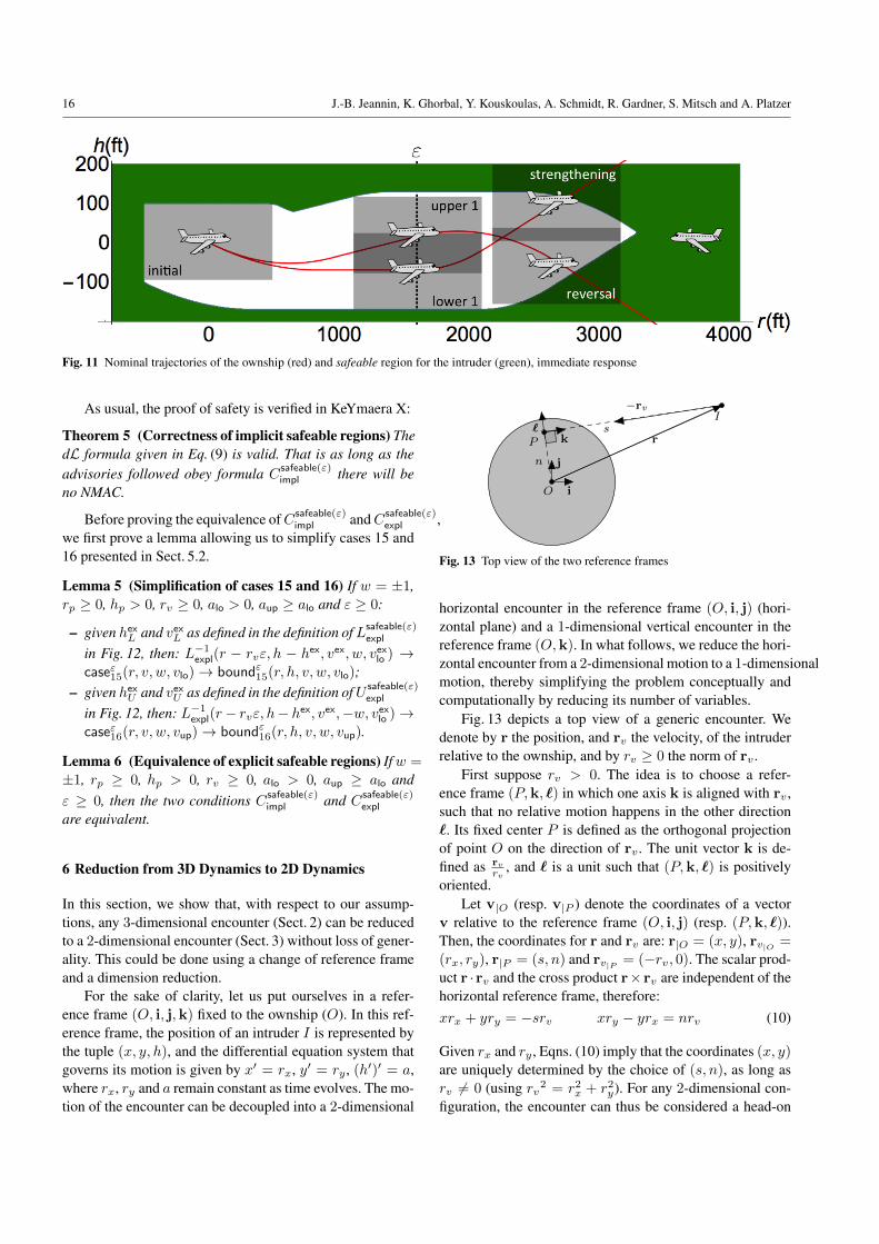
in Fig. 11: we consider all the positions and speeds at whichthe ownship can end up at time ε, and in particular the lowestsuch position and speed (position lower 1), and the highestsuch position and speed (position upper 1). At the lowest po-sition, we look at the most extreme strengthening available;and at the highest position, we look at the most extremereversal available. The disjunction of the two safe regionsof this strengthening and of this reversal corresponds to in-truder positions that can be avoided by an appropriate actionat time ε: this is the safeable region. Another way of seeingsafeable is that it is a subset of bounded-time safe that also
provides liveness of the model: it ensures that the ownshipdoes not get stuck at time ε.
The safeable formulation is presented in Fig. 12, and agraphic representation in Fig. 11. Throughout this sectionwe suppose that ε ≥ 0, i.e., all the safe regions not explicitlylabelled as non-bounded-time (with superscript −1) have afinite time bound.
5.3.1 Model The model is presented in Eq. (9), and buildson the bounded-time model Eq. (8), with very few changes.
1 rp ≥ 0 ∧ hp > 0 ∧ rv ≥ 0 ∧ alo > 0 ∧ aup ≥ alo2 ∧ ε ≥ 0 ∧ (w = −1 ∨ w = 1)
3 ∧Csafeable(ε)impl (r, h, v, w, vlo, v
exlo , vup, v
exup)→
4 [( ( (w := −1 ∪ w := 1); vlo := ∗; vup := ∗;5 ?C
safeable(ε)impl (r, h, v, w, vlo, v
exlo , vup, v
exup);
6 advisory := (w, vlo, vup) );
7 t := 0;
8 ( a := ∗;9 {r′ = −rv, h′ = −v, v′ = a, t′ = 1 & t ≤ ε10 ∧ (wv ≥ wvlo ∨ wa ≥ alo)11 ∧ ((wv ≤ wvup ∧ wa ≤ aup) ∨ wa ≤ 0)
12 } )∗13 )∗] (|r| > rp ∨ |h| > hp)
(9)
In fact, we are only changing the conditions toCsafeable(ε)impl
on lines 2 and 4. But that makes a big difference: informally,instead of having a model that gets stuck at time ε, we nowhave a model that can always find a safeable advisory (al-though we don’t formally prove that last fact yet).
5.3.2 Implicit and explicit formulations of the safeableregions The formulations presented in Fig. 12 use the for-mulations of the bounded-time safe regions as building blocks.The implicit and explicit formulations are built in very sim-ilar ways.
As shown in Fig. 11, the nominal lower bound trajectoryconsists of a bounded-time lower bound trajectory startingat time 0, followed by an unbounded-time lower bound tra-jectory starting at time ε; this nominal trajectory is at heighthex and vertical velocity vex at time ε. Therefore the safe-able lower bound consists of one bounded-time lower boundup to time ε, followed by an unbounded-time lower boundstarting at time ε, height hexL and vertical velocity vexL .
The nominal upper bound trajectory consists, however,of a bounded-time upper bound trajectory starting at time 0,followed by an unbounded time reversed (i.e., taking −w)lower bound trajectory starting at time ε; this nominal trajec-tory is at height hex and vertical velocity vex at time ε. There-fore the safeable upper bound consists of one bounded-timelower bound up to time ε, followed by an unbounded-timelower bound starting at time ε, height hexU and vertical veloc-ity vexU .
16 J.-B. Jeannin, K. Ghorbal, Y. Kouskoulas, A. Schmidt, R. Gardner, S. Mitsch and A. Platzer
Fig. 11 Nominal trajectories of the ownship (red) and safeable region for the intruder (green), immediate response
As usual, the proof of safety is verified in KeYmaera X:
Theorem 5 (Correctness of implicit safeable regions) ThedL formula given in Eq. (9) is valid. That is as long as theadvisories followed obey formula Csafeable(ε)
impl there will beno NMAC.
Before proving the equivalence ofCsafeable(ε)impl andCsafeable(ε)
expl ,we first prove a lemma allowing us to simplify cases 15 and16 presented in Sect. 5.2.
Lemma 5 (Simplification of cases 15 and 16) If w = ±1,rp ≥ 0, hp > 0, rv ≥ 0, alo > 0, aup ≥ alo and ε ≥ 0:
– given hexL and vexL as defined in the definition ofLsafeable(ε)expl
in Fig. 12, then: L−1expl(r − rvε, h − hex, vex, w, vexlo ) →caseε15(r, v, w, vlo)→ boundε15(r, h, v, w, vlo);
– given hexU and vexU as defined in the definition ofU safeable(ε)expl
in Fig. 12, then: L−1expl(r− rvε, h− hex, vex,−w, vexlo )→caseε16(r, v, w, vup)→ boundε16(r, h, v, w, vup).
Lemma 6 (Equivalence of explicit safeable regions) Ifw =
±1, rp ≥ 0, hp > 0, rv ≥ 0, alo > 0, aup ≥ alo andε ≥ 0, then the two conditions Csafeable(ε)
impl and Csafeable(ε)expl
are equivalent.
6 Reduction from 3D Dynamics to 2D Dynamics
In this section, we show that, with respect to our assump-tions, any 3-dimensional encounter (Sect. 2) can be reducedto a 2-dimensional encounter (Sect. 3) without loss of gener-ality. This could be done using a change of reference frameand a dimension reduction.
For the sake of clarity, let us put ourselves in a refer-ence frame (O, i, j,k) fixed to the ownship (O). In this ref-erence frame, the position of an intruder I is represented bythe tuple (x, y, h), and the differential equation system thatgoverns its motion is given by x′ = rx, y′ = ry , (h′)′ = a,where rx, ry and a remain constant as time evolves. The mo-tion of the encounter can be decoupled into a 2-dimensional
O
I
r
−rv
i
j
k`P
s
n
Fig. 13 Top view of the two reference frames
horizontal encounter in the reference frame (O, i, j) (hori-zontal plane) and a 1-dimensional vertical encounter in thereference frame (O,k). In what follows, we reduce the hori-zontal encounter from a 2-dimensional motion to a 1-dimensionalmotion, thereby simplifying the problem conceptually andcomputationally by reducing its number of variables.
Fig. 13 depicts a top view of a generic encounter. Wedenote by r the position, and rv the velocity, of the intruderrelative to the ownship, and by rv ≥ 0 the norm of rv .
First suppose rv > 0. The idea is to choose a refer-ence frame (P,k, `) in which one axis k is aligned with rv ,such that no relative motion happens in the other direction`. Its fixed center P is defined as the orthogonal projectionof point O on the direction of rv . The unit vector k is de-fined as rv
rv, and ` is a unit such that (P,k, `) is positively
oriented.Let v|O (resp. v|P ) denote the coordinates of a vector
v relative to the reference frame (O, i, j) (resp. (P,k, `)).Then, the coordinates for r and rv are: r|O = (x, y), rv|O =
(rx, ry), r|P = (s, n) and rv|P = (−rv, 0). The scalar prod-uct r ·rv and the cross product r×rv are independent of thehorizontal reference frame, therefore:xrx + yry = −srv xry − yrx = nrv (10)
Given rx and ry , Eqns. (10) imply that the coordinates (x, y)are uniquely determined by the choice of (s, n), as long asrv 6= 0 (using rv2 = r2x + r2y). For any 2-dimensional con-figuration, the encounter can thus be considered a head-on

A Formally Verified Hybrid System for Safe Advisories in the Next-Generation Airborne Collision Avoidance System 17
Implicit formulation
Lsafeable(ε)impl (r, h, v, w, vlo, v
exlo ) ≡ L
εimpl(r, h, v, w, vlo) ∧(
∀hexL .∀vexL .
(0 ≤ ε <
max(0, w(vlo − v))alo
∧ hexL =walo
2ε2 + vloε ∧ vexL = waloε+ v
∨ ε ≥max(0, w(vlo − v))
alo∧ hexL = vloε−
wmax(0, w(vlo − v))2
2alo∧ vexL = vlo
)→ L−1
impl(r − rvε, h− hexL , v
exL , w, v
exlo )
)U
safeable(ε)impl (r, h, v, w, vup, v
exup) ≡ Uε
impl(r, h, v, w, vup) ∧(∀hexU .∀v
exU .
(0 ≤ ε <
max(0, w(vup − v))aup
∧ hexU =waup
2ε2 + vupε ∧ vexU = waupε+ v
∨ ε ≥max(0, w(vup − v))
aup∧ hexU = wmax(wvup, wv)ε−
wmax(0, w(vup − v))2
2aup∧ vexU = wmax(wvup, wv)
)→ L−1
impl(r − rvε, h− hexU , v
exU ,−w, v
exup)
)C
safeable(ε)impl (r, h, v, w, vlo, vexlo , vup, v
exup) ≡ L
safeable(ε)impl (r, h, v, w, vlo, vexlo ) ∨ U
safeable(ε)impl (r, h, v, w, vup, vexup)
Explicit formulation
Lsafeable(ε)expl (r, h, v, w, vlo, v
exlo ) ≡ L
εexpl(r, h, v, w, vlo) ∧ L
−1expl(r − rvε, h− h
exL , v
exL , w, v
exlo )
where
hexL =
walo
2ε2 + vloε and vexL = waloε+ v if 0 ≤ ε <
max(0, w(vlo − v))alo
hexL = vloε−wmax(0, w(vlo − v))2
2aloand vexL = vlo if ε ≥
max(0, w(vlo − v))alo
Usafeable(ε)expl (r, h, v, w, vup, v
exup) ≡ Uε
expl(r, h, v, w, vup) ∧ L−1expl(r − rvε, h− h
exU , v
exU ,−w, v
exup)
where
hexU =
waup
2ε2 + vupε and vexU = waupε+ v if 0 ≤ ε <
max(0, w(vup − v))aup
hexU = wmax(wvup, wv)ε−wmax(0, w(vup − v))2
2aupand vexU = wmax(wvup, wv) if ε ≥
max(0, w(vup − v))aup
Csafeable(ε)expl (r, h, v, w, vlo, vexlo , vup, v
exup) ≡ L
safeable(ε)expl (r, h, v, w, vlo, vexlo ) ∨ U
safeable(ε)expl (r, h, v, w, vup, vexup)
Fig. 12 Implicit and explicit formulations of the safeable region
encounter where s plays the role of r and where a new puckradius, denoted sp, plays the role of rp.
Let us now determine the radius sp of the dimension-reduced encounter, and prove that the absence of NMAC in(O, i, j)—characterized by r2 > r2p—is equivalent to theabsence of NMAC in (P,k, `)—characterized by s2 > s2p.Using (10):
rv2r2 = rv
2(x2 + y2) = (xrx + yry)2 + (xry − yrx)2
= rv2(s2 + n2) .
Since rv 6= 0, this implies r2 = s2+n2. Therefore, r2 > r2pif and only if s2 + n2 > r2p or equivalently s2 > r2p −n2. If r2p − n2 < 0, the direction of the vector rv does notintersect the puck, the inequality s2 > r2p − n2 is triviallytrue, and the encounter is safe. If r2p−n2 ≥ 0, we choose thenew puck radius sp for the dimension-reduced encounter assp =
√rp2 − n2 ≥ 0, and the safety condition in (P,k, `)
becomes s2 ≥ s2p. When θv = 180◦, one has s = r, n = 0
and sp = rp as in Sect. 3–4.
As the encounter evolves in (O, i, j) along x′ = rx, y′ =
ry , its dimension-reduced version evolves in (P,k, `) alongthe differential equations s′ = −rv, n′ = 0, obtained bydifferentiating Eqns. (10) and canceling rv . The followingproposition, proved in KeYmaera, combines both dynamicsand shows that the absence of an NMAC of radius rp in(O, i, j) is equivalent to the absence of an NMAC of radiussp in (P,k, `).
Proposition 1 (Horizontal Reduction) The following dLformula is valid(xrx + yry = −srv ∧ xry − yrx = nrv∧x2 + y2 = n2 + s2 ∧ rv2 = r2x + r2y
)→ [x′ = rx, y
′ = ry, s′ = −rv, n′ = 0](
x2 + y2 > r2p ↔ s2 > r2p − n2)
(11)
Observe that the horizontal NMAC condition in (P,k, `)
only depends on the change of one variable rather than two.The proposition also applies to the special case rv = 0. Inthis case the origin P is no longer defined, and Eqns. (10)

18 J.-B. Jeannin, K. Ghorbal, Y. Kouskoulas, A. Schmidt, R. Gardner, S. Mitsch and A. Platzer
are trivially true. The variables s and n are constants (s′ =0, n′ = 0), their initial values are only restricted by the con-dition n2 + s2 = x2 + y2 in the assumption of the propo-sition, but they are not unique. When the relative positionbetween the two aircraft does not evolve over time, if the in-truder is at a safe distance initially, the encounter is still safefor all time.
7 Tightness of Conditions
The conditions L−1impl and L−1expl in Fig. 3, Ddimpl and Dd
expl in
Fig. 5, and Csafeable(ε)impl and Csafeable(ε)
expl in Fig. 12 specify con-ditions we have derived for safety under varying assump-tions. While we have formally proved that each of theseconditions is sufficient to guarantee safety within the rele-vant models (Theorem 1, Corollary 1, Theorem 2, Lemma 2,Theorem 5, and Lemma 6), we have not proved that theseconditions are necessary for safety or tight. I.e., if an advi-sory and aircraft geometry meet the safety conditions, thenthe aircraft are guaranteed to be safe under the relevant as-sumptions. However, we have not proved that advisories arenot safe when that advisory and the associated geometry donot meet the conditions.
In some cases, our conditions are overapproximations.For the conditions that do not account for subsequent ad-visories (safe conditions), L−1impl/L
−1expl and Dd
impl/Ddexpl, con-
sider the following physically unreliable geometry. The air-craft are diverging horizontally (e.g., θv = 0 and rv > 0),the intruder is sufficiently above the ownship in altitude, i.e.,more than hp above the ownship (h > hp), and the aircraftare horizontally separated by exactly the radius of the puck,i.e., r = rp. Intuitively, the intruder is directly above the leftedge of the gray box in Fig. 4. If considering an up-senseadvisory, this geometry does not pass L−1expl or Dd
expl becausethe conditions have no exception for intruders over the exactedge of the puck. However, NMAC would require the own-ship to accelerate upward at an infinite rate, so NMAC is notpossible.
There are cases where advisories fail to meet the con-ditions for subsequent advisories (safeable conditions), butare safe under the relevant assumptions as well. ConditionsC
safeable(ε)impl /Csafeable(ε)
expl are built from a lower-bound trajec-tory and an upper-bound trajectory where, e.g., the lower-bound trajectory ends with an unbounded-time trajectorycorresponding to the strongest possible upward subsequentadvisory (vertical velocity vex). Such construction forms areasonable overapproximation under the intuition that if thestrongest upward subsequent advisory makes the lower-boundinitial-trajectory safe, that subsequent advisory would alsomake any other initial-trajectory safe. Analogous reason-ing supports the construction of the upper-bound trajectory.The limitation of this approach, with respect to complete-
ness, is that it implicitly assumes that the subsequent advi-sory is fixed, or determined at the time of the first advisory.I.e., it asks if there exists one subsequent advisory now (atleast either the most extreme upward or downward advisory)that can guarantee safety in the future. In reality, ACAS Xchooses the subsequent advisory later in time, with someknowledge of the initial portion of the trajectory. In somecases, it is advantageous, for example, to choose the mostextreme downward advisory for lower initial trajectories andto choose the most extreme upward advisory for upper ini-tial trajectories. The result of this overapproximation is thatACAS X could always choose a safe subsequent advisoryfor some geometries that cannot be concluded safeable byC
safeable(ε)impl /Csafeable(ε)
expl .
8 Comparison of Safety Theorems to ACAS X
The preceding theorems about safety are independent of thetested system. To characterize the safety of ACAS X itself,we check whether advisories indicated by the core com-ponent of ACAS X, consisting of the timing and logic ta-bles, meet the conditions of the theorems. The timing andlogic tables of ACAS X contain scores for each advisoryfor a set of discrete sample states. Each score quantifiesthe desirability of issuing the corresponding advisory whenin the corresponding state and is the result of optimizing aMarkov decision process (MDP). In practice, ACAS X mul-tilinearly interpolates advisory scores from the values storedin the tables, given estimates of aircraft states. Althoughthese estimates model uncertainty in practice, we check be-havior for the sample points themselves, assuming perfectknowledge of state, to compare system behavior under best-case circumstances. Table 2 shows the range of sample statepoints, called cut-points, for each of the 7 dimensions of thelogic tables. These non-uniformly sampled cut-points werechosen by the ACAS X designers to maximize system per-formance for realistic encounters while keeping the size ofthe tables modest. The previous advisory state includes thepreviously-issued advisory and information about whetherthe pilot was acting to comply with the advisory at the previ-ous time step. This information is used in the MDP state forthe multi-step optimization. Together these samples makeup over 648 billion state combinations for which scores areexplicitly stored in the ACAS X logic tables.
Corollary 1 and Lemma 6 along with Theorem 5 reducethe safety of all future trajectories to a static condition onthe current state: L−1expl or Csafeable(ε)
expl , respectively. We ex-amine the advisory specified by the logic tables at each ofthe 648 billion state combinations for which scores are ex-plicitly stored and check the advisory against the respectivesafe or safeable condition for that advisory.

A Formally Verified Hybrid System for Safe Advisories in the Next-Generation Airborne Collision Avoidance System 19
parameter samples range of values
relative alt. h (ft) 45 [-8000, -4000, -3600, -3200, -2800, -2400, -2000, . . . , -100, -50, 0, 50, . . . , 4000, 8000]ownship alt. rate v (ft/s) 25 [-166.7, -83.3, -75.0, -66.7, -58.3, -50, . . . , -16.7, -8.3, -4.2, 0, 4.2, . . . , 83.3, 166.7]intruder alt. rate vI (ft/s) 25 [-166.7, -83.3, -75.0, -66.7, -58.3, -50, . . . , -16.7, -8.3, -4.2, 0, 4.2, . . . , 83.3, 166.7]previous advisory 33 { NONE-NONE, DNC2000-NONE, DNC2000-DNC2000, . . . , SCL2500-NONE, SCL2500-SCL2500 }range r (ft) 101 [0, 50, 100, 150, 200, 250, 300, . . . , 1000, 1500, 2000, . . . , 39500, 40000, 100000, 200000]relative velocity rv (ft/s) 187 [0, 10, 20, 30, 40, 50, 60, 70, 80, 90 . . . , 1700, 1750, 1800, . . . , 2350, 2400, 2450, 2500]velocity angle θv (deg) 37 [0, 5, 10, 15, 20, 25, 30, 35, 40, 45, . . . , 145, 150, 155, 160, 165, 170, 175, 180]
Table 2 Discrete parameter ranges and number of cut-points specified by ACAS X run 13 and checked during comparison
δ (seconds) ε (seconds) ad ∆a = aup − alo0 1 g/106 01 2 g/6 g/123 5 g/3 g/65 7 g/2 g/4
Table 3 Delay and Acceleration Parameters Swept During LogicComparison. Delay pairs (left) are tied together, while accelerationpairs (right) are tied. The 16 combinations of these pairs are tested.
Approach. To perform the comparison we use a 10-nodecluster, each with 48 cores and 128 GB RAM. Checks forthe relevant conditions are implemented in Julia 2 and runon the 648 billion cut-point combinations in parallel, takingapproximately 8 days. We first define what we mean by acounterexample.
Definition 1 (Counterexample) We say that a state is a coun-terexample for the safe (resp. safeable) conditions if the ad-visory given by the ACAS X logic tables for that state vio-lates L−1expl given in Fig. 3 (resp. Csafeable(ε)
expl given in Fig. 12)and for which there exists an alternative advisory that doessatisfy the respective safety conditions.
We say a state is non-safe, or non-safeable if it is a coun-terexample for the safe or safeable conditions respectively.
We selected a set of parameters for acceleration and de-lay ranges, shown in Table 3. The delays are parameterizedby two values δ and ε. The first, δ, is the delay from time0 to the time at which the pilot begins adjusting vertical ac-celeration to follow the first advisory. The second delay pa-rameter, ε, is the delay from time 0 to the time at which thesecond issued advisory begins to be followed. Thus the firstadvisory is followed for ε − δ seconds and we require thatε > δ. The selections of delay parameters in Table 3 have εvalues that are at least 1 second greater than δ to allow a pe-riod of 1 second or more of compliance with a first advisory.The right side of Table 3 gives the parameters governing thelimits of ownship acceleration. The free acceleration, ad, aspreviously defined, is the maximum absolute acceleration ofthe pilot during delay or COC; it is swept between almostzero acceleration and g/2. (We used g/106 for almost zeroto avoid divisions by zero in our conditions.) The second
2 http://julialang.org.
Safe Counterexamples(in billions) delay (δ, ε) in secondsacceleration (ad,∆a) (0, 1) (1, 2) (3, 5) (5, 7)
(g/106, 0) 15.38 15.05 14.85 14.79(g/6, g/12) 15.40 15.03 14.87 14.88(g/3, g/6) 15.43 15.02 14.95 15.14(g/2, g/4) 15.45 15.01 15.18 15.33
Unresolvable States(in billions) delay (δ, ε) in secondsacceleration (ad,∆a) (0, 1) (1, 2) (3, 5) (5, 7)
(g/106, 0) 10.42 10.64 10.84 10.96(g/6, g/12) 10.42 10.75 11.16 11.51(g/3, g/6) 10.42 10.88 11.59 12.36(g/2, g/4) 10.42 11.04 12.13 13.46
Table 4 Number of Safe counterexamples (top) and number of unre-solvable states (bottom) for each delay and acceleration parameter set
parameter, ∆a, the overcompliance acceleration, is the dif-ference between the upper limit of acceleration under theadvisory, aup, and the lower compliance limit, alo. It is tiedin each case to one half of the free acceleration ad. The de-lay parameter pairs are also tied together during each query,meaning that during the first query (δ, ε) = (0, 1) and forthe second query (δ, ε) = (0, 2), and so on. All 16 combina-tions of delay pairs and acceleration pairs are tested againstthe total 648 billion cut-point combinations summarized inTable 2.
Counterexamples. Tables 4 and 5 summarize the numberof counterexamples (Def. 1) we found. The lower portionsof the tables show the number of initial states tested thatwere not resolvable with any of the available safe or safe-able actions. That is, for those unresolvable states, there areno available advisories that pass the conditions we formallyproved. For the safe comparison, the checks we perform arelimited to states in the ACAS X tables where COC is theprevious advisory (about 196 billion states). In addition, theparameters ε and ∆a are not used in the safe conditions: εis fixed to −1 as we assume that the pilot will follow the is-sued advisory forever; ∆a is not used as we assume that thevertical acceleration has only to respect a minimal rate (alo)to satisfy the advisory. Thus, only δ and ad vary. One cannotice that taking into account the pilot delay in the formal

20 J.-B. Jeannin, K. Ghorbal, Y. Kouskoulas, A. Schmidt, R. Gardner, S. Mitsch and A. Platzer
SafeableCounterexamples(in millions) delay (δ, ε) in secondsacceleration (ad,∆a) (0, 1) (1, 2) (3, 5) (5, 7)
(g/106, 0) 266.3 99.7 39.2 31.6(g/6, g/12) 310.0 117.2 101.4 164.9(g/3, g/6) 353.2 138.6 277.7 544.7(g/2, g/4) 398.9 163.6 668.8 898.7
Unresolvable States(in billions) delay (δ, ε) in secondsacceleration (ad,∆a) (0, 1) (1, 2) (3, 5) (5, 7)
(g/106, 0) 11.03 11.27 11.51 11.64(g/6, g/12) 11.03 11.40 11.85 12.23(g/3, g/6) 11.03 11.54 12.30 13.09(g/2, g/4) 11.03 11.71 12.86 14.23
Table 5 Number of Safeable counterexamples (top) and unresolvablestates (bottom) for each delay and acceleration parameter set
model reduces the number of counterexamples. This mayseem at first counterintuitive as one expects less unsafe ad-visories if the pilot responds immediately. However, giventhat the previous advisory is a COC, the ACAS X tables aredesigned to not necessarily issue a disruptive advisory rightaway and will rather either issue a preventive advisory (suchas DNC or DND) or simply a MAINTAIN before actuallystrengthening those advisories in the future if needed. Thosefirst advisories may indeed violate the safe conditions al-though the system is able to resolve the potential encounters.We also observe, on the contrary, that increasing the freeacceleration ad results in more counterexamples and moreunresolvable encounters. This is a straightforward effect ofour worst case analysis: if we allow g/2, say, as worst casevertical acceleration, then we have to consider that the pilotwill actually accelerate at g/2 during the delay, which maybe unrealistic.
Overall, as shown in Table 4, we found billions of coun-terexamples to Corollary 1 (safe regions). Many were usedto create test encounters and tested in the full system as ameans of targeted stress testing. As alluded to earlier, theACAS X system was able to resolve many of those by is-suing subsequent advisories, which actually motivated thesafeable extension we developed in this paper. Indeed, safe-able counterexamples represent states where the advice givenby ACAS X may not be correctable by subsequent advi-sories, although an alternative guaranteed safe sequence ex-ists for our assumptions according to Lemma 6.
We can see from Table 5 that there are considerably fewersafeable counterexamples than safe ones, hundreds of mil-lions instead of tens of billions. Theorem 5 (safeable regions)is designed to detect points of no return. As with safe re-gions, we see that the number of counterexamples tend tohave an inverse relationship with pilot response delay al-though an exception to this trend occurs when delay is ex-
actly 0. We believe this exception is caused by the fact thatmany states are resolvable when there is no pilot responsedelay, i.e., when the pilot responds immediately to the is-sued advice. Once a moderate response delay is assumed,there are many fewer resolvable initial states, resulting infewer total counterexamples, albeit still a few hundred mil-lion. These safeable counterexamples are also being used togenerate stressing short-time encounters that may be usedfor robustness testing.
Safety Analysis. The comparison of the system to safe con-dition D−1expl (valid by Theorem 2) gave insight into possibleimprovements for ACAS X. Our analysis led to the identifi-cation of unexpected behavior in the ACAS X run 13 (i.e.,version 13) lookup tables. In some cases, the ACAS X advi-sory seems to induce an NMAC, i.e., if the initial advisory isfollowed and not strengthened or reverted later, an NMACwill occur when it would not have occurred if the aircraftcontinued flying straight. A typical example, found duringchecking against Corollary 1 (safe regions) with δ = 0 andad = g/2, is shown in Fig. 14. The ownship is flying fromthe left and the intruder from the right. The time 0 corre-sponds to the time of closest horizontal approach. As timeprogresses, the intruder flies towards the ownship and anNMAC happens near the time t = 0. The original path of theownship does not lead to an NMAC. However, ACAS X is-sues a Do-Not-Climb advisory. If the pilot follows this advi-sory immediately and stops climbing, and if the initial advi-sory is not subsequently strengthened or reversed, an NMACwill occur.
In other cases of counterexamples to Corollary 1 (saferegions), the advisory does not seem to have any benefit.In those cases, flying at the vertical rates disallowed by theadvisory would actually avoid NMAC, while not all allowedvertical rates of the advisory are safe.
Some safe counterexamples are tolerated, as ACAS Xtries to minimize alerting the pilot unless it has to do so;for these cases, ACAS X will issue or strengthen an advi-sory later to avoid issuing a disruptive alert immediately.Additionally, the assumption of straight vertical flight is notalways valid. E.g., aircraft may actually be more likely tolevel-off than continue at high vertical rates in some cases.The particular unexpected behavior shown in Fig. 14 was in-dependently identified by the ACAS X team using simulation-based testing, and is being addressed in a subsequent revi-sion of the system.
Safeable Analysis. In Fig. 15, we see an automatically dis-covered safeable counterexample. The pilot is assumed tostart complying with the initially issued advisory at 5 sec-onds and will only begin complying with a potential subse-quent advisory after 7 seconds from the initial time (the firstadvisory will thus be followed for 2 seconds). For this state,
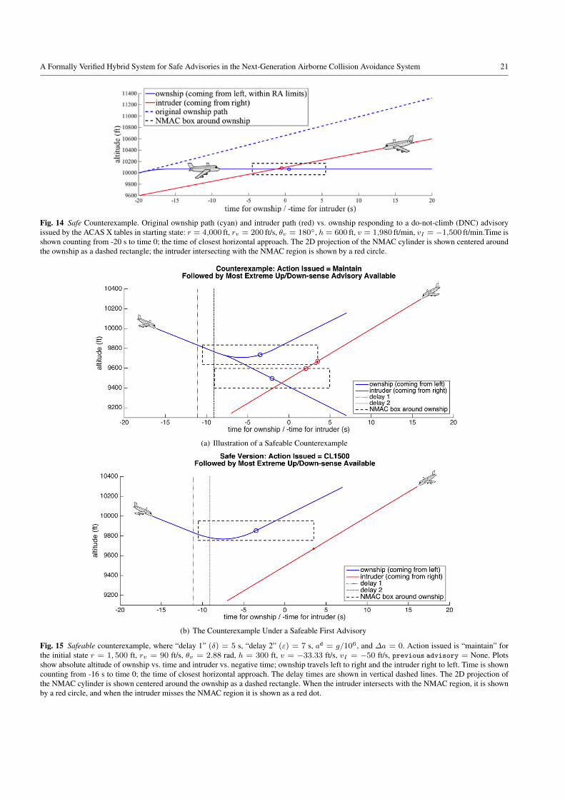
A Formally Verified Hybrid System for Safe Advisories in the Next-Generation Airborne Collision Avoidance System 21
Fig. 14 Safe Counterexample. Original ownship path (cyan) and intruder path (red) vs. ownship responding to a do-not-climb (DNC) advisoryissued by the ACAS X tables in starting state: r = 4,000 ft, rv = 200 ft/s, θv = 180◦, h = 600 ft, v = 1,980 ft/min, vI = −1,500 ft/min.Time isshown counting from -20 s to time 0; the time of closest horizontal approach. The 2D projection of the NMAC cylinder is shown centered aroundthe ownship as a dashed rectangle; the intruder intersecting with the NMAC region is shown by a red circle.
(a) Illustration of a Safeable Counterexample
(b) The Counterexample Under a Safeable First Advisory
Fig. 15 Safeable counterexample, where “delay 1” (δ) = 5 s, “delay 2” (ε) = 7 s, ad = g/106, and ∆a = 0. Action issued is “maintain” forthe initial state r = 1, 500 ft, rv = 90 ft/s, θv = 2.88 rad, h = 300 ft, v = −33.33 ft/s, vI = −50 ft/s, previous advisory = None. Plotsshow absolute altitude of ownship vs. time and intruder vs. negative time; ownship travels left to right and the intruder right to left. Time is showncounting from -16 s to time 0; the time of closest horizontal approach. The delay times are shown in vertical dashed lines. The 2D projection ofthe NMAC cylinder is shown centered around the ownship as a dashed rectangle. When the intruder intersects with the NMAC region, it is shownby a red circle, and when the intruder misses the NMAC region it is shown as a red dot.

22 J.-B. Jeannin, K. Ghorbal, Y. Kouskoulas, A. Schmidt, R. Gardner, S. Mitsch and A. Platzer
the ACAS X tables issue the advisory MDES, maintain de-scent. The upper panel shows the most extreme upper andlower paths that a subsequent advisory can restrict the own-ship’s motion to. Neither of these can avoid NMAC withthe intruder. This is a relatively close range, slow closingencounter, as the initial horizontal separation is 1,500 feetand horizontal relative closing speed is only 90 feet/second.Both aircraft begin descending at moderate rates, offset ver-tically by 300 feet. The problem occurs because the mostextreme descend advisory available has a rate of only 2500feet/minute and with the ownship already descending at 2000feet/minute the increase in descent rate cannot avoid the in-truder. In this slow closing geometry, the two aircraft will bein horizontal conflict range for an extended period, which atthis geometry lasts for 7 seconds starting at t = −3.5 to t =3.5 seconds. In this case, Lemma 6 tells us that safeable ac-tions include Do-Not-Descend and Climb-1500. The lowerpanel of Fig. 15 shows that if the ownship were, instead, toldto climb at the maximum rates allowed by a sequence of up-sense advisories, this situation would have been resolved,and so is indeed a counterexample.
The smaller number of safeable counterexamples are ofspecial interest to system verification, as they are situationsthat cannot even be corrected by subsequent advisories. Toaid in robustness testing and tuning of the actual system,we have created a set of short-time encounters based on thecounterexamples found using the safeable analysis and aresharing these encounters with the ACAS X designers.
Overall, we have begun analyzing ACAS X using ourtheorem and are identifying numerous valuable outcomes.These results either help us characterize tradeoffs being madeor help us identify undesirable behaviors in the system. Asone of our next steps, we aim to prove that ACAS X givessafe advice for continuous regions of the state space. Whencomparisons are extended to check contiguous regions ofthe state space, our approach will have the potential for acomplete analysis of the system over all potential encounterconfigurations, thereby reducing vulnerability to the sam-pling of encounter scenarios.
9 Related Work
Kochenderfer and Chryssanthacopoulos [13] describe the de-sign of the ACAS X lookup-tables. Their principled approach,based on optimizing an MDP, guarantees the selection of op-timal advisories according to a cost model. The state spaceand dynamics are discretized. Their notion of optimality de-pends on costs assigned to various events.
Holland et al. [11] and Chludzinski [1] simulate largenumbers of encounters, including tracks from recorded flightdata, to evaluate the performance of ACAS X. These simu-lations account for high-fidelity details of an encounter, but
they only cover a finite set of the continuous state space withno formal guarantees.
Von Essen and Giannakopoulou [3] use probabilistic model-checking to analyze an MDP based on [13]. They investigatethe probability of several undesirable events occurring. Be-cause they ostensibly analyze an MDP, their work inheritsmany of the assumptions of ACAS X, including errors dueto discretized dynamics. Their analysis depends heavily onthe MDP considered and thus needs to be redone on everyversion of ACAS X.
Lygeros and Lynch [18] use hybrid techniques to for-mally verify the TCAS conflict resolution algorithms. Theyassume—rather than prove—that TCAS ends up in a statewhere one aircraft has a climbing advisory and the othera descending advisory. They then prove (by hand) a lowerbound on the vertical separation of both aircraft at the pointof closest approach. In contrast, we do prove as opposed toassume that and when advisories are safe.
Tomlin et al. [24], Platzer and Clarke [23], Loos et al. [17]and Ghorbal et al. [10] use hybrid systems approaches todesign safe horizontal maneuvers for collision avoidance.Dowek et al. [2] and Galdino et al. [9] describe and ver-ify in the PVS theorem prover a collision avoidance systemof their design called KB3D.
Overall, our approach is different from previous comple-mentary work in that:
– unlike [3,13], we rely on an independent model from theone used to design ACAS X;
– unlike [2,9,10,17,23,24] we analyze an independent in-dustrial system and not a safe-by-design system;
– unlike [2,3,9] our analysis uses realistic, continuous dy-namics;
– unlike [18,24] we provide universal safe regions that canbe reused for new versions of ACAS X or new systems;
– unlike [1,11,14,18,24], we provide mechanized rigor-ous proofs of correctness of our model.
10 Conclusion and Future Work
We developed a general strategy for analyzing the safetyof complicated, real-world aircraft collision avoidance sys-tems, and applied it to ACAS X. Our strategy identifies saferegions where an advisory is proved to always keep the air-craft clear of NMAC, under some assumptions. We identi-fied states where ACAS X is provably safe, and deliveredothers showing unexpected behaviors back to the ACAS Xdevelopment team. The identified safe regions are indepen-dent from the version of ACAS X and can thus be reused forfuture versions. In future work, we plan to extend our hybridmodel to account for curved trajectories of both aircraft aswell as vertical acceleration of the intruder.

A Formally Verified Hybrid System for Safe Advisories in the Next-Generation Airborne Collision Avoidance System 23
Acknowledgments. This research was conducted under thesponsorship of the Federal Aviation Administration TrafficAlert & Collision Avoidance System (TCAS) Program Of-fice (PO) AJM-233 under contract number DTFAWA-11-C-00074. Additionally, support for the basic verification tech-nology used as a foundation for this research was providedby the National Science Foundation under NSF CAREERAward CNS-1054246.
The authors would like to warmly thank Neal Suchy forhis lead of the ACAS X project and support of this work,as well as Nathan Fulton, Ran Ji and Jan-David Quesel fortheir support of the KeYmaera tool. The authors would alsolike to thank Jeff Brush, Barbara Chludzinski, Dane Fichter,Jessica Holland, Robert Klaus, Barbara Kobzik-Juul, MykelKochenderfer, Ted Londner, Sarah Loos, Jessica Lopez, EdMorehouse, Wes Olson, Michael Owen, Anshu Saksena, JoshuaSilbermann, and the ACAS X development team for inter-esting discussions and remarks.
References
1. Chludzinski, B.J.: Evaluation of TCAS II version 7.1 using theFAA fast-time encounter generator model. Tech. Rep. ATC-346,MIT Lincoln Laboratory (2009)
2. Dowek, G., Munoz, C., Carreno, V.: Provably safe coordinatedstrategy for distributed conflict resolution. In: AIAA GuidanceNavigation, and Control Conference and Exhibit (2005)
3. von Essen, C., Giannakopoulou, D.: Analyzing the next genera-tion airborne collision avoidance system. In: TACAS, LNCS, vol.8413, pp. 620–635. Springer (2014).
4. Federal Aviation Administration: Introduction to TCAS II (2011).Version 7.1
5. Federal Aviation Administration TCAS Program Office: Algo-rithm design description for the surveillance and tracking moduleof ACAS X (2014). Run12
6. Federal Aviation Administration TCAS Program Office: Algo-rithm design description for the threat resolution module of ACASX (2014). Version 3 Rev. 1
7. Felty, A., Middeldorp, A. (eds.): International Conference on Au-tomated Deduction, CADE’15, Berlin, Germany, Proceedings,LNCS, vol. 9195. Springer (2015)
8. Fulton, N., Mitsch, S., Quesel, J.D., Volp, M., Platzer, A.: KeY-maera X: An axiomatic tactical theorem prover for hybrid systems.In: Felty and Middeldorp [7], pp. 527–538.
9. Galdino, A., Munoz, C., Ayala, M.: Formal verification of an op-timal air traffic conflict resolution and recovery algorithm. In:WoLLIC, LNCS, vol. 4576. Springer (2007)
10. Ghorbal, K., Jeannin, J.B., Zawadzki, E., Platzer, A., Gordon, G.J.,Capell, P.: Hybrid theorem proving of aerospace systems: Appli-cations and challenges. Journal of Aerospace Information Systems(2014)
11. Holland, J.E., Kochenderfer, M.J., Olson, W.A.: Optimizing thenext generation collision avoidance system for safe, suitable, andacceptable operational performance. Air Traffic Control Quarterly(2014)
12. Jeannin, J.B., Ghorbal, K., Kouskoulas, Y., Gardner, R., Schmidt,A., Zawadzki, E., Platzer, A.: A formally verified hybrid systemfor the next-generation airborne collision avoidance system. In:C. Baier, C. Tinelli (eds.) TACAS, LNCS, vol. 9035, pp. 21–36.Springer (2015).
13. Kochenderfer, M.J., Chryssanthacopoulos, J.P.: Robust airbornecollision avoidance through dynamic programming. Tech. Rep.ATC-371, MIT Lincoln Laboratory (2010)
14. Kochenderfer, M.J., Espindle, L.P., Kuchar, J.K., Griffith, J.D.:Correlated encounter model for cooperative aircraft in the nationalairspace system version 1.0. Tech. Rep. ATC-344, MIT LincolnLaboratory (2008)
15. Kochenderfer, M.J., Holland, J.E., Chryssanthacopoulos, J.P.:Next generation airborne collision avoidance system. LincolnLaboratory Journal 19(1), 17–33 (2012)
16. Kochenderfer, M.J., Monath, N.: Compression of optimal valuefunctions for Markov decision processes. In: Data CompressionConference. Snowbird, Utah (2013)
17. Loos, S.M., Renshaw, D.W., Platzer, A.: Formal verification ofdistributed aircraft controllers. In: HSCC, pp. 125–130. ACM(2013).
18. Lygeros, J., Lynch, N.: On the formal verification of the TCASconflict resolution algorithms. In: IEEE Decision and Control,vol. 2, pp. 1829–1834. IEEE (1997).
19. Platzer, A.: Differential dynamic logic for hybrid systems. J. Au-tom. Reas. 41(2), 143–189 (2008).
20. Platzer, A.: Logical Analysis of Hybrid Systems: Proving Theo-rems for Complex Dynamics. Springer (2010).
21. Platzer, A.: Logics of dynamical systems. In: LICS, pp. 13–24.IEEE (2012).
22. Platzer, A.: A uniform substitution calculus for differential dy-namic logic. In: Felty and Middeldorp [7], pp. 467–481.
23. Platzer, A., Clarke, E.M.: Formal verification of curved flight col-lision avoidance maneuvers: A case study. In: FM, LNCS, vol.5850, pp. 547–562. Springer (2009).
24. Tomlin, C., Pappas, G.J., Sastry, S.: Conflict resolution for air traf-fic management: A study in multiagent hybrid systems. AutomaticControl, IEEE Transactions on 43(4), 509–521 (1998)