BPEA Conference Drafts, March 7–8, 2019

A Forensic Examination of China’s National Accounts

Wei Chen, Chinese University of Hong Kong

Xilu Chen, Chinese University of Hong Kong

Chang-Tai Hsieh, University of Chicago

Zheng (Michael) Song, Chinese University of Hong Kong

Conflict of Interest Disclosure: Chang-Tai Hsieh is the Phyllis and Irwin Winkelried Professor of Economics at the University of Chicago; Wei Chen and Xilu Chen are students, and Zheng (Michael) Song is a Distinguished Visiting Professor at Tsinghua University and Professor at the Department of Economics of the Chinese University of Hong Kong, where Wei Chen and Xilu Chen are also PhD students. Beyond these affiliations, Dr. Song received financial support from the General Research Council of Hong Kong, and the remaining authors did not receive financial support from any firm or person for this paper or from any firm or person with a financial or political interest in this paper. They are currently not officers, directors, or board members of any organization with an interest in this paper. No outside party had the right to review this paper before circulation. The views expressed in this paper are those of the authors, and do not necessarily reflect those of the University of Chicago, Tsinghua University, or the Chinese University of Hong Kong.

1  

A Forensic Examination of China’s National Accounts*

Wei Chen Chinese University of Hong Kong

Xilu Chen Chinese University of Hong Kong

Chang-Tai Hsieh University of Chicago and NBER

Zheng (Michael) Song Chinese University of Hong Kong

Prepared for the March 2019 BPEA Panel

Abstract

China’s national accounts are based on data collected by local governments. However, since local governments are rewarded for meeting growth and investment targets, they have an incentive to skew local statistics. China’s National Bureau of Statistics (NBS) adjusts the data provided by local governments to calculate GDP at the national level. The adjustments made by the NBS average 5% of GDP since the mid-2000s. On the production side, the discrepancy between local and aggregate GDP is entirely driven by the gap between local and national estimates of industrial output. On the expenditure side, the gap is in investment. Local statistics increasingly misrepresent the true numbers after 2008, but there was no corresponding change in the adjustment made by the NBS. We provide revised estimates of local and national GDP by re-estimating output of industrial, wholesale, and retail firms using data on value-added taxes. We also use several local economic indicators that are less likely to be manipulated by local governments to estimate local and aggregate GDP. The estimates also suggest that the adjustments by the NBS were insufficient after 2008. Relative to the official numbers, we estimate that GDP growth from 2008-2016 is 1.7 percentage points lower and the investment and savings rate in 2016 is 7 percentage points lower.

                                                            * We thank David Dollar, Jan Eberly, and Wei Xiong for helpful comments. We are also grateful to Chong-en Bai and numerous current and former officials of China’s National Bureau of Statistics and local statistical bureaus for many helpful discussions.

2  

1. Introduction

China’s national accounts are primarily based on data compiled by local officials.

However, as documented by Xiong (2018), local officials are rewarded for meeting growth

and investment targets. Therefore, it is not surprising that local governments also have an

incentive to skew the statistics on local growth and investment. The Statistical Agency of the

Chinese government, the National Bureau of Statistics (NBS henceforth), attempts to correct

this bias by adjusting local statistics using data from their own surveys and administrative

data. The accuracy of the final numbers of aggregate GDP and its components depends on

the extent of misreporting by local officials, the data that NBS has at its disposal to correct

the misreporting, and the effort it undertakes to do so.

Local GDP is measured via the production approach from three major surveys (of

large industrial sector firms, large service sector firms, and “qualified” construction firms).

This data is supplemented with surveys of smaller industrial firms and administrative data

from other government departments to obtain a number for local GDP. On the expenditure

side, local officials provide estimates of local consumption, investment, government

spending, and net exports (vis-à-vis other localities in China and outside of China). The two

main sources are surveys of household income and expenditures (similar to the US CEX),

from which they estimate local consumption, and survey data on investment projects. Since

the sum of local consumption and investment typically exceeds local GDP measured on the

production side, the residual is attributed to net exports. But to be clear, local net exports is

simply calculated as a residual and is not based on any data.

The NBS has access to the micro-data of the surveys used by local governments and

supplements this data with economic censuses and administrative data such as land sales,

vehicle registration and foreign trade. On the former, for example, NBS conducted a census

of industrial firms in 1995 and censuses of all firms (in all sectors) in 2004, 2008, 2013, and

2018 (although the latter has not yet been processed). Based on this data, it adjusts the

reports by local governments to arrive at a number for national GDP and its components on

the production and expenditure sides.

We then check which of the numbers provided by local governments are more likely

to be inaccurate. First, we show that the sum of local GDP frequently exceeds national GDP.

Second, we compare the sum of the local consumption, investment, and net exports with

national consumption, investment and net exports reported by the National Bureau of

3  

Statistics. We find little discrepancy between local and national consumption, but find a

large discrepancy between local and national statistics of investment and net exports. Third,

we compare the sum of value-added of sectors as reported at the local level with the same

sectors at the national level. We find large discrepancies for the industrial sector and smaller

gaps in the non-industrial sectors.

We then use two approaches to determine the accuracy of adjustments to the local

numbers by the NBS. First, we adjust national GDP by the difference between value added

growth reported by NBS and value added tax revenue growth reported by the State

Administration of Taxation in the sectors where value added tax is a major type of taxation.

Our estimate suggests that the adjustments made by the National Bureau of Statistics were

roughly accurate until 2007/8. However, the adjustments made after this date no longer

appear to be accurate. Our baseline estimate of GDP growth from 2008 to 2016 is 1.7

percentage points lower than the official growth rate. Furthermore, our estimate of the

aggregate investment and savings rate in 2016 is 7 percentage points lower than the official

numbers.

We use the same approach to adjust local production and expenditure GDP for each

Chinese province. There is a strong positive relation between our adjustments to local GDP

and investment across provinces, with a correlation of 0.61. This evidence suggests that local

governments inflate local GDP by overestimating local production as well as local

investment.

A second approach is to estimate a statistical model where we estimate the

relationship between a set of economic indicators (which are less likely to be manipulated)

and local GDP prior to 2008. We then use parameters of the estimated model along with the

same set of the indicators after 2008 to predict local GDP after 2008. The indicators include

satellite night lights, national tax revenue, electricity consumption, railway cargo flow,

exports and imports. We use the method developed by Su, Shi and Phillips (2016) to control

for (hidden) economic structure heterogeneities across regions. Using this method, we also

find that the corrections made to national GDP no longer appear appropriate after 2008.

In summary, our revised numbers of the Chinese national accounts indicate that the

slowdown in Chinese growth since 2008 is more severe than suggested by the official

statistics. On the other hand, the true savings rate has probably declined by 10 percentage

points from 2008 to 2016, with about two-thirds of the savings decline showing up in the

4  

external surplus and the remainder in the investment rate. In this sense, our revised numbers

of the national accounts also indicate that Chinese growth is now more associated with

consumption rather than investment and external surpluses.

2. China’s GDP Accounting System

A key institutional feature of the Chinese National Accounts is that the underlying

data are compiled by statistical bureaus of local governments. Local statistical bureaus use

this data to provide estimates of local GDP and its components on the production and

expenditure sides. The National Bureau of Statistics (NBS) of the Chinese central

government use the estimates of local GDP, along with data it collects independently, to

arrive at a number for national GDP. The number provided by the NBS is the “official”

number of Chinese GDP.

Although the local statistical bureaus are technically branches of the NBS and are

supposed to follow the statistical procedures set by the NBS, local officers of the statistical

bureau are evaluated and promoted by the local government. Because of this hierarchical

structure, local statistical bureaus are susceptible to pressure by local officials who may have

an incentive to report inaccurate statistics. The NBS is aware of this bias and adjusts the

numbers of local GDP provided by the local statistical bureaus.

To assess the quality of the official numbers for local and national GDP, we proceed

in three steps. First, we compare the sum of local GDP with aggregate GDP provided by the

NBS (hereafter, we use the term aggregate GDP to refer to the number provided by the

Central Government’s NBS). Second, we assess the data used to estimate GDP on the

production side. Third, we assess the data used to construct GDP on the expenditure data.

2.1 Comparing Local GDP with Aggregate GDP

The solid line in Panel A of Figure 1 shows the magnitude of the adjustment made by

the NBS to the local statistics. The figure shows the gap between the sum of GDP of each

province and aggregate GDP provided by the NBS as a fraction of aggregate GDP. Local

governments understated GDP relative to the NBS in the 1990s. The sum of local GDP was

about five to six% lower than aggregate GDP in the mid-1990s. This pattern was reversed

5  

after 2003. After this date the sum of local GDP surpassed aggregate GDP and was 6%

higher than aggregate GDP in 2006. The gap between these two numbers for China’s GDP

stabilized around 5% after 2006.

[Insert Figure 1]

Local statistical authorities and the NBS also provide estimates of local and aggregate

GDP by broad sectors. Figure 1 shows the gap between the sum of local GDP and aggregate

GDP of each sector as a share of aggregate GDP (of all sectors). The top panel in Figure 1

shows the ratio of the sum of local GDP to aggregate GDP for agriculture (“primary”),

industry and construction (“secondary”), and services (“tertiary”). Prior to 2003, the sum of

secondary GDP at the local level was lower than aggregate secondary GDP. Furthermore,

from about 1997 to 2003 almost all the gap between local and aggregate GDP came from the

gap in the industrial sector. Prior to 1997, some of the gap is due to the discrepancy between

local and aggregate statistics of the service sector.

After 2003 all of the discrepancy between local and aggregate GDP comes from the

industrial sector. The bottom panel in Figure 1 shows the comparison of industrial (mining,

manufacturing, and public utilities) and construction GDP reported by local governments

with that provided by the NBS. As can be seen, the gap between local and national statistics

after 2003 is entirely in industry. This finding echoes those by Holtz (2014) and Ma et. al.

(2014), who also show that the inconsistency between provincial and national GDP mainly

came from the industrial sector,

Figure 2 compares GDP expenditures provided by local governments and the NBS.

On the expenditure side, there are substantial differences after 2003 in investment (“Gross

Fixed Capital Formation”) and net exports reported by the two sources. The sum of local

investment was close to the national level until 2002. After that, the sum of local investment

has exceeded aggregate investment. In 2016 the gap in the two measures of investment

reached 13% of GDP. The mirror image is the growing discrepancy between the sum of local

net exports and aggregate net exports. This gap reached 8% of GDP in 2016. In contrast, the

national and local differences in final consumption and changes in inventory are essentially

zero after the mid-2000s.1

                                                            1 Final consumption includes urban and rural household consumption and government consumption. The sum of each of the local consumption component is very close to its national counterpart.

6  

[Insert Figure 2]

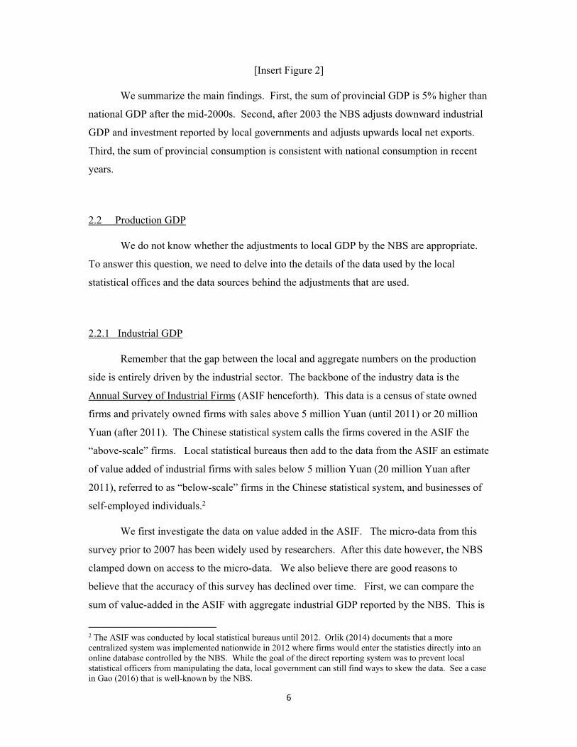
We summarize the main findings. First, the sum of provincial GDP is 5% higher than

national GDP after the mid-2000s. Second, after 2003 the NBS adjusts downward industrial

GDP and investment reported by local governments and adjusts upwards local net exports.

Third, the sum of provincial consumption is consistent with national consumption in recent

years.

2.2 Production GDP

We do not know whether the adjustments to local GDP by the NBS are appropriate.

To answer this question, we need to delve into the details of the data used by the local

statistical offices and the data sources behind the adjustments that are used.

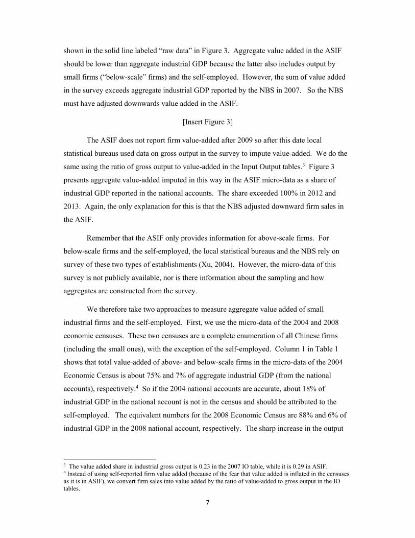
2.2.1 Industrial GDP

Remember that the gap between the local and aggregate numbers on the production

side is entirely driven by the industrial sector. The backbone of the industry data is the

Annual Survey of Industrial Firms (ASIF henceforth). This data is a census of state owned

firms and privately owned firms with sales above 5 million Yuan (until 2011) or 20 million

Yuan (after 2011). The Chinese statistical system calls the firms covered in the ASIF the

“above-scale” firms. Local statistical bureaus then add to the data from the ASIF an estimate

of value added of industrial firms with sales below 5 million Yuan (20 million Yuan after

2011), referred to as “below-scale” firms in the Chinese statistical system, and businesses of

self-employed individuals.2

We first investigate the data on value added in the ASIF. The micro-data from this

survey prior to 2007 has been widely used by researchers. After this date however, the NBS

clamped down on access to the micro-data. We also believe there are good reasons to

believe that the accuracy of this survey has declined over time. First, we can compare the

sum of value-added in the ASIF with aggregate industrial GDP reported by the NBS. This is

                                                            2 The ASIF was conducted by local statistical bureaus until 2012. Orlik (2014) documents that a more centralized system was implemented nationwide in 2012 where firms would enter the statistics directly into an online database controlled by the NBS. While the goal of the direct reporting system was to prevent local statistical officers from manipulating the data, local government can still find ways to skew the data. See a case in Gao (2016) that is well-known by the NBS.

7  

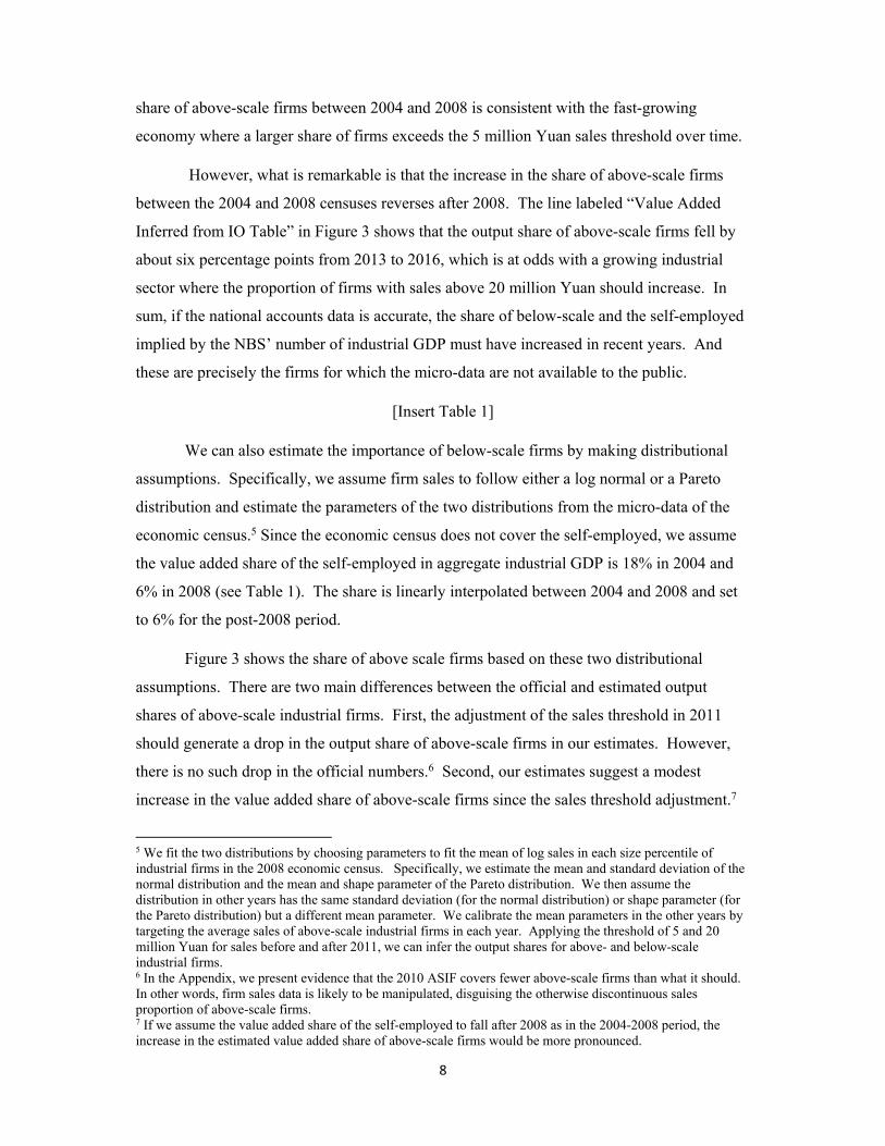
shown in the solid line labeled “raw data” in Figure 3. Aggregate value added in the ASIF

should be lower than aggregate industrial GDP because the latter also includes output by

small firms (“below-scale” firms) and the self-employed. However, the sum of value added

in the survey exceeds aggregate industrial GDP reported by the NBS in 2007. So the NBS

must have adjusted downwards value added in the ASIF.

[Insert Figure 3]

The ASIF does not report firm value-added after 2009 so after this date local

statistical bureaus used data on gross output in the survey to impute value-added. We do the

same using the ratio of gross output to value-added in the Input Output tables.3 Figure 3

presents aggregate value-added imputed in this way in the ASIF micro-data as a share of

industrial GDP reported in the national accounts. The share exceeded 100% in 2012 and

2013. Again, the only explanation for this is that the NBS adjusted downward firm sales in

the ASIF.

Remember that the ASIF only provides information for above-scale firms. For

below-scale firms and the self-employed, the local statistical bureaus and the NBS rely on

survey of these two types of establishments (Xu, 2004). However, the micro-data of this

survey is not publicly available, nor is there information about the sampling and how

aggregates are constructed from the survey.

We therefore take two approaches to measure aggregate value added of small

industrial firms and the self-employed. First, we use the micro-data of the 2004 and 2008

economic censuses. These two censuses are a complete enumeration of all Chinese firms

(including the small ones), with the exception of the self-employed. Column 1 in Table 1

shows that total value-added of above- and below-scale firms in the micro-data of the 2004

Economic Census is about 75% and 7% of aggregate industrial GDP (from the national

accounts), respectively.4 So if the 2004 national accounts are accurate, about 18% of

industrial GDP in the national account is not in the census and should be attributed to the

self-employed. The equivalent numbers for the 2008 Economic Census are 88% and 6% of

industrial GDP in the 2008 national account, respectively. The sharp increase in the output

                                                            3 The value added share in industrial gross output is 0.23 in the 2007 IO table, while it is 0.29 in ASIF. 4 Instead of using self-reported firm value added (because of the fear that value added is inflated in the censuses as it is in ASIF), we convert firm sales into value added by the ratio of value-added to gross output in the IO tables.

8  

share of above-scale firms between 2004 and 2008 is consistent with the fast-growing

economy where a larger share of firms exceeds the 5 million Yuan sales threshold over time.

However, what is remarkable is that the increase in the share of above-scale firms

between the 2004 and 2008 censuses reverses after 2008. The line labeled “Value Added

Inferred from IO Table” in Figure 3 shows that the output share of above-scale firms fell by

about six percentage points from 2013 to 2016, which is at odds with a growing industrial

sector where the proportion of firms with sales above 20 million Yuan should increase. In

sum, if the national accounts data is accurate, the share of below-scale and the self-employed

implied by the NBS’ number of industrial GDP must have increased in recent years. And

these are precisely the firms for which the micro-data are not available to the public.

[Insert Table 1]

We can also estimate the importance of below-scale firms by making distributional

assumptions. Specifically, we assume firm sales to follow either a log normal or a Pareto

distribution and estimate the parameters of the two distributions from the micro-data of the

economic census.5 Since the economic census does not cover the self-employed, we assume

the value added share of the self-employed in aggregate industrial GDP is 18% in 2004 and

6% in 2008 (see Table 1). The share is linearly interpolated between 2004 and 2008 and set

to 6% for the post-2008 period.

Figure 3 shows the share of above scale firms based on these two distributional

assumptions. There are two main differences between the official and estimated output

shares of above-scale industrial firms. First, the adjustment of the sales threshold in 2011

should generate a drop in the output share of above-scale firms in our estimates. However,

there is no such drop in the official numbers.6 Second, our estimates suggest a modest

increase in the value added share of above-scale firms since the sales threshold adjustment.7

                                                            5 We fit the two distributions by choosing parameters to fit the mean of log sales in each size percentile of industrial firms in the 2008 economic census. Specifically, we estimate the mean and standard deviation of the normal distribution and the mean and shape parameter of the Pareto distribution. We then assume the distribution in other years has the same standard deviation (for the normal distribution) or shape parameter (for the Pareto distribution) but a different mean parameter. We calibrate the mean parameters in the other years by targeting the average sales of above-scale industrial firms in each year. Applying the threshold of 5 and 20 million Yuan for sales before and after 2011, we can infer the output shares for above- and below-scale industrial firms. 6 In the Appendix, we present evidence that the 2010 ASIF covers fewer above-scale firms than what it should. In other words, firm sales data is likely to be manipulated, disguising the otherwise discontinuous sales proportion of above-scale firms. 7 If we assume the value added share of the self-employed to fall after 2008 as in the 2004-2008 period, the increase in the estimated value added share of above-scale firms would be more pronounced.

9  

In contrast, the share declined after 2012 in the official numbers, which does not seem

plausible.

Another way to gauge whether the accuracy of the NBS’ estimate of industrial GDP is

to use information on revenues from value added taxes on industrial firms. China imposes a

17% value added tax on essentially all industrial firms. The main exception is that some

industrial goods are subject to a 13% value added tax. We show in the Appendix that the

compositional change of high- and low-tax goods has no effect on the growth of value added

tax revenues. Second, a significant proportion of domestic industrial value added tax (41% in

2015) is refundable through export tax rebates, which varied considerably across goods and

over time. To make sure that our estimates are not affected by tax rebates, we will use data

on revenues from value-added taxes gross of rebates for exports.

The State Administration of Taxation (SAT) implemented the so-called “Golden

Taxation Project” since 1994, making tax fraud and evasion difficult. A computerized

taxation data network has been in full operation since 2005, which allows the tax authorities

to cross-check the input and output value added tax at each stage of production and

distribution of goods and services (Xu, 2011). In addition, even if there is some fraud and

evasion, as long as their degree does not increase, revenues from the value-added tax on

industrial firms should be proportional to industrial GDP.

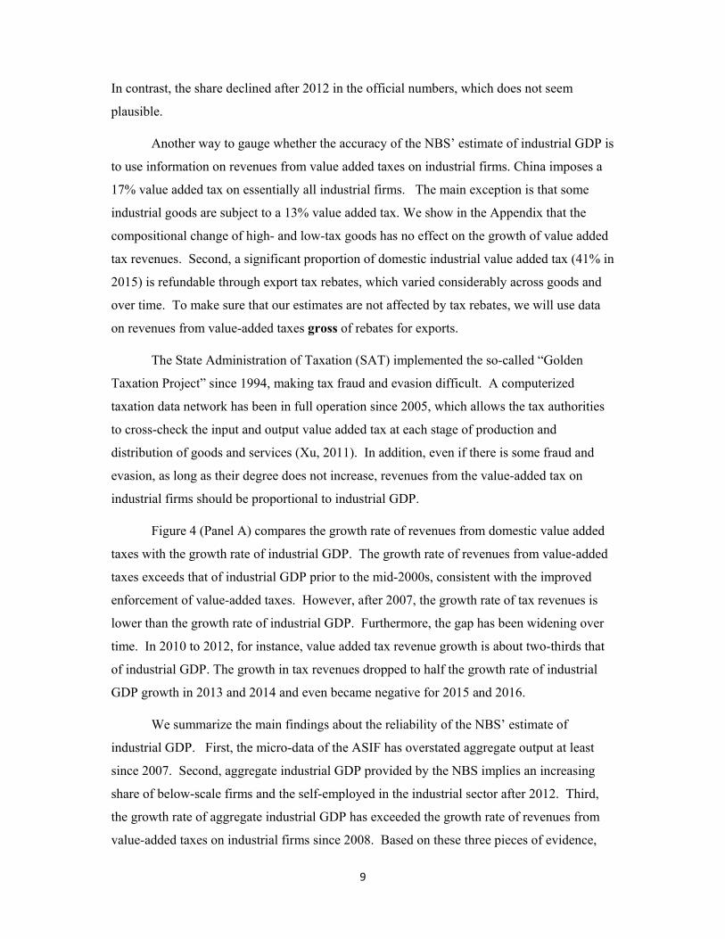
Figure 4 (Panel A) compares the growth rate of revenues from domestic value added

taxes with the growth rate of industrial GDP. The growth rate of revenues from value-added

taxes exceeds that of industrial GDP prior to the mid-2000s, consistent with the improved

enforcement of value-added taxes. However, after 2007, the growth rate of tax revenues is

lower than the growth rate of industrial GDP. Furthermore, the gap has been widening over

time. In 2010 to 2012, for instance, value added tax revenue growth is about two-thirds that

of industrial GDP. The growth in tax revenues dropped to half the growth rate of industrial

GDP growth in 2013 and 2014 and even became negative for 2015 and 2016.

We summarize the main findings about the reliability of the NBS’ estimate of

industrial GDP. First, the micro-data of the ASIF has overstated aggregate output at least

since 2007. Second, aggregate industrial GDP provided by the NBS implies an increasing

share of below-scale firms and the self-employed in the industrial sector after 2012. Third,

the growth rate of aggregate industrial GDP has exceeded the growth rate of revenues from

value-added taxes on industrial firms since 2008. Based on these three pieces of evidence,

10  

we conclude that despite the adjustments made by the NBS to local industrial GDP, the

official numbers of aggregate industrial GDP – and by extension aggregate GDP for all

sectors -- is likely to overstate the truth after 2007/8.

[Insert Figure 4]

2.2.2 Non-Industrial GDP

Turning to the non-industrial sector, NBS conducts surveys for all “qualified”

construction firms, above-scale wholesale and retail firms, above-scale hotel and catering

firms, and all real estate developers and operators.8 We first look into the wholesale and

retail sectors, which accounted for about 10% of aggregate GDP in 2016. While the published

tabulations of the surveys provide total sales of above-scale wholesale and retail firms, value

added is not reported. We thus convert total sales to value-added, following the procedure in

Bai et al. (2019) that uses firm survey data from China’s State Administration of Taxation.9

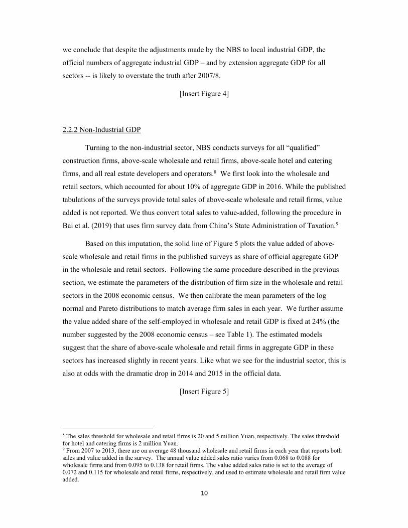
Based on this imputation, the solid line of Figure 5 plots the value added of above-

scale wholesale and retail firms in the published surveys as share of official aggregate GDP

in the wholesale and retail sectors. Following the same procedure described in the previous

section, we estimate the parameters of the distribution of firm size in the wholesale and retail

sectors in the 2008 economic census. We then calibrate the mean parameters of the log

normal and Pareto distributions to match average firm sales in each year. We further assume

the value added share of the self-employed in wholesale and retail GDP is fixed at 24% (the

number suggested by the 2008 economic census – see Table 1). The estimated models

suggest that the share of above-scale wholesale and retail firms in aggregate GDP in these

sectors has increased slightly in recent years. Like what we see for the industrial sector, this is

also at odds with the dramatic drop in 2014 and 2015 in the official data.

[Insert Figure 5]

                                                            8 The sales threshold for wholesale and retail firms is 20 and 5 million Yuan, respectively. The sales threshold for hotel and catering firms is 2 million Yuan. 9 From 2007 to 2013, there are on average 48 thousand wholesale and retail firms in each year that reports both sales and value added in the survey. The annual value added sales ratio varies from 0.068 to 0.088 for wholesale firms and from 0.095 to 0.138 for retail firms. The value added sales ratio is set to the average of 0.072 and 0.115 for wholesale and retail firms, respectively, and used to estimate wholesale and retail firm value added.

11  

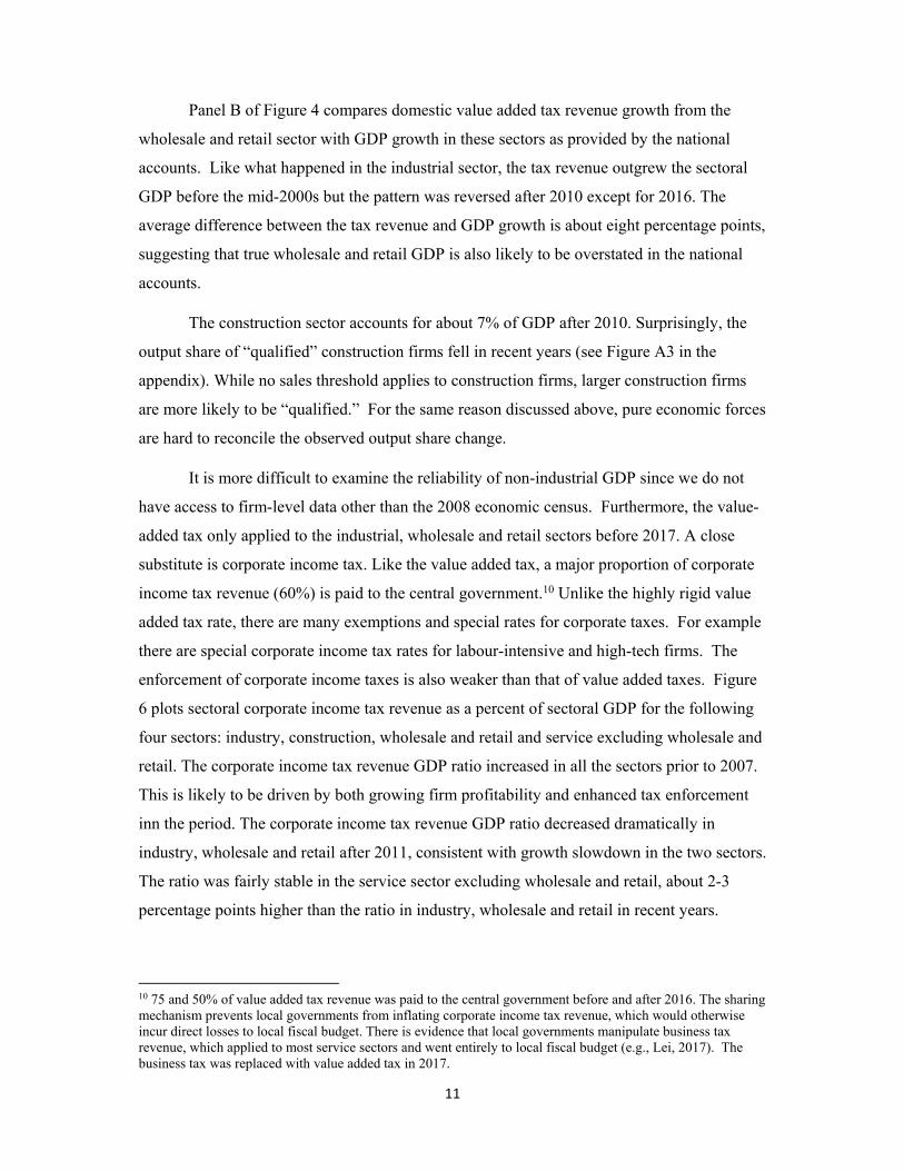
Panel B of Figure 4 compares domestic value added tax revenue growth from the

wholesale and retail sector with GDP growth in these sectors as provided by the national

accounts. Like what happened in the industrial sector, the tax revenue outgrew the sectoral

GDP before the mid-2000s but the pattern was reversed after 2010 except for 2016. The

average difference between the tax revenue and GDP growth is about eight percentage points,

suggesting that true wholesale and retail GDP is also likely to be overstated in the national

accounts.

The construction sector accounts for about 7% of GDP after 2010. Surprisingly, the

output share of “qualified” construction firms fell in recent years (see Figure A3 in the

appendix). While no sales threshold applies to construction firms, larger construction firms

are more likely to be “qualified.” For the same reason discussed above, pure economic forces

are hard to reconcile the observed output share change.

It is more difficult to examine the reliability of non-industrial GDP since we do not

have access to firm-level data other than the 2008 economic census. Furthermore, the value-

added tax only applied to the industrial, wholesale and retail sectors before 2017. A close

substitute is corporate income tax. Like the value added tax, a major proportion of corporate

income tax revenue (60%) is paid to the central government.10 Unlike the highly rigid value

added tax rate, there are many exemptions and special rates for corporate taxes. For example

there are special corporate income tax rates for labour-intensive and high-tech firms. The

enforcement of corporate income taxes is also weaker than that of value added taxes. Figure

6 plots sectoral corporate income tax revenue as a percent of sectoral GDP for the following

four sectors: industry, construction, wholesale and retail and service excluding wholesale and

retail. The corporate income tax revenue GDP ratio increased in all the sectors prior to 2007.

This is likely to be driven by both growing firm profitability and enhanced tax enforcement

inn the period. The corporate income tax revenue GDP ratio decreased dramatically in

industry, wholesale and retail after 2011, consistent with growth slowdown in the two sectors.

The ratio was fairly stable in the service sector excluding wholesale and retail, about 2-3

percentage points higher than the ratio in industry, wholesale and retail in recent years.

                                                            10 75 and 50% of value added tax revenue was paid to the central government before and after 2016. The sharing mechanism prevents local governments from inflating corporate income tax revenue, which would otherwise incur direct losses to local fiscal budget. There is evidence that local governments manipulate business tax revenue, which applied to most service sectors and went entirely to local fiscal budget (e.g., Lei, 2017). The business tax was replaced with value added tax in 2017.

12  

Construction is the only sector where the corporate income tax GDP ratio kept increasing

until 2015.

[Insert Figure 6 and 7]

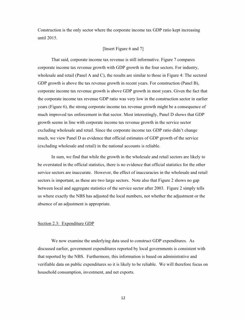
That said, corporate income tax revenue is still informative. Figure 7 compares

corporate income tax revenue growth with GDP growth in the four sectors. For industry,

wholesale and retail (Panel A and C), the results are similar to those in Figure 4: The sectoral

GDP growth is above the tax revenue growth in recent years. For construction (Panel B),

corporate income tax revenue growth is above GDP growth in most years. Given the fact that

the corporate income tax revenue GDP ratio was very low in the construction sector in earlier

years (Figure 6), the strong corporate income tax revenue growth might be a consequence of

much improved tax enforcement in that sector. Most interestingly, Panel D shows that GDP

growth seems in line with corporate income tax revenue growth in the service sector

excluding wholesale and retail. Since the corporate income tax GDP ratio didn’t change

much, we view Panel D as evidence that official estimates of GDP growth of the service

(excluding wholesale and retail) in the national accounts is reliable.

In sum, we find that while the growth in the wholesale and retail sectors are likely to

be overstated in the official statistics, there is no evidence that official statistics for the other

service sectors are inaccurate. However, the effect of inaccuracies in the wholesale and retail

sectors is important, as these are two large sectors. Note also that Figure 2 shows no gap

between local and aggregate statistics of the service sector after 2003. Figure 2 simply tells

us where exactly the NBS has adjusted the local numbers, not whether the adjustment or the

absence of an adjustment is appropriate.

Section 2.3: Expenditure GDP

We now examine the underlying data used to construct GDP expenditures. As

discussed earlier, government expenditures reported by local governments is consistent with

that reported by the NBS. Furthermore, this information is based on administrative and

verifiable data on public expenditures so it is likely to be reliable. We will therefore focus on

household consumption, investment, and net exports.

13  

The backbone of aggregate household consumption are the urban and rural household

surveys. The local statistical bureaus and the NBS directly take aggregates of household

spending on food, clothing, household facilities, education, culture and recreation services,

miscellaneous goods and services. The other components of household consumption also use

the Household Surveys but are adjusted for (i) accounting discrepancies (i.e., medical

expenditure paid by government is not in the Household Survey but is included in final

consumption); (ii) biases in the surveys (i.e., rich households are under-represented in the

Household Survey). Xu (2014) describes in detail how the NBS arrives at consumption

aggregates by adjusting the data from the Household Survey. The adjustments are based on

administrative data from the relevant government departments. For instance, NBS uses social

security income and expenditure data to adjust medical expenditure. Another example is to

use the production, sales and import data of automobiles from the Association of Automobile

Industry and the Department of Public Security (where all new automobiles are registered) to

adjust consumption on transportation and communication. This helps to correct the bias

caused by under-represented rich households who are more likely to purchase automobiles.

Investment spending is officially called “Fixed Capital Formation” (FCF) in the

Chinese national accounts. This data is primarily based on reports of fixed asset investment

(FAI) by local governments. FAI includes expenditures on land purchases and used capital,

so local statistical authorities use a survey of land purchases and used capital to subtract these

two items from FAI to arrive at a number for FCF.

However, there is abundant evidence that the FAI has become more unreliable. In

contrast with ASIF which is based on firm’s financial statement, FAI is based on reports of

investment projects by local governments. There is no audit of this data, nor are there any

consequences for misreporting this information. In addition to the incentive of local officials

to misreport this number, tax considerations may also lead to the inflation of FAI.11 In 2013

Xu Xianchun, a Vice Director of NBS at the time, publicly stated that that FAI is inflated by

local statistical offices (Xu, 2014). According to him, “some regions set up unrealistic

investment targets for sub regions and use them as indicators of performance evaluation” (pp.

4).

                                                            11 For instance, the Ministry of Finance and the State Administration of Taxation introduced a policy (Notice of the Ministry of Finance and the State Administration of Taxation on Several Issues concerning the National Implementation of Value-added Tax Reform, No. 170, 2008, the Ministry of Finance) that allows tax payers to deduct fixed asset investment from value-added tax.

14  

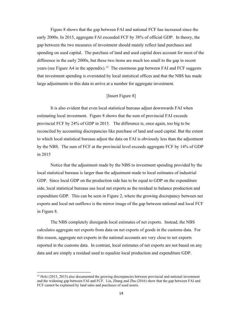
Figure 8 shows that the gap between FAI and national FCF has increased since the

early 2000s. In 2015, aggregate FAI exceeded FCF by 38% of official GDP. In theory, the

gap between the two measures of investment should mainly reflect land purchases and

spending on used capital. The purchase of land and used capital does account for most of the

difference in the early 2000s, but these two items are much too small to the gap in recent

years (see Figure A4 in the appendix).12 The enormous gap between FAI and FCF suggests

that investment spending is overstated by local statistical offices and that the NBS has made

large adjustments to this data to arrive at a number for aggregate investment.

[Insert Figure 8]

It is also evident that even local statistical bureaus adjust downwards FAI when

estimating local investment. Figure 8 shows that the sum of provincial FAI exceeds

provincial FCF by 24% of GDP in 2015. The difference is, once again, too big to be

reconciled by accounting discrepancies like purchase of land and used capital. But the extent

to which local statistical bureaus adjust the data on FAI is obviously less than the adjustment

by the NBS. The sum of FCF at the provincial level exceeds aggregate FCF by 14% of GDP

in 2015

Notice that the adjustment made by the NBS to investment spending provided by the

local statistical bureaus is larger than the adjustment made to local estimates of industrial

GDP. Since local GDP on the production side has to be equal to GDP on the expenditure

side, local statistical bureaus use local net exports as the residual to balance production and

expenditure GDP. This can be seen in Figure 2, where the growing discrepancy between net

exports and local net outflows is the mirror image of the gap between national and local FCF

in Figure 8.

The NBS completely disregards local estimates of net exports. Instead, the NBS

calculates aggregate net exports from data on net exports of goods in the customs data. For

this reason, aggregate net exports in the national accounts are very close to net exports

reported in the customs data. In contrast, local estimates of net exports are not based on any

data and are simply a residual used to equalize local production and expenditure GDP.

                                                            12 Holz (2013, 2015) also documented the growing discrepancies between provincial and national investment and the widening gap between FAI and FCF. Liu, Zhang and Zhu (2016) show that the gap between FAI and FCF cannot be explained by land sales and purchases of used assets.

15  

We summarize the main findings. Local statistical bureaus inflate investment and, to

a smaller extent, output in the industrial, wholesale, and retail sectors. Since investment data

is easier to manipulate (the amount of investment is project-specific and disconnected to

investing firms’ financial statement), the misstatement of investment spending is more severe

than the bias in GDP. The gap between the two are “reconciled” by the large net inflows of

goods and services reported by local governments. In contrast, consumption data based on

household surveys is more reliable.

3. Revised Estimates of GDP Growth

The obvious question then is what are the “true” estimates of China’s GDP growth?

Here we make two efforts to come up with a number. First, we use alternative data from tax

records to generate alternative measures of GDP on the production side. We then use them to

re-estimate aggregate investment as well as local GDP. Second, we take a data fitting

approach and use external data that are not likely to be manipulated by local governments to

estimate GDP.

Section 3.1: Adjusting National Accounts with Tax Data

Our first approach to estimate “true” GDP is built on the following three assumptions.

First, we assume industrial output reported by local statistical officers has not been reliable

since the late 2000s. Second, we assume industrial value added tax revenue is proportional

to true industrial value added. Third, we assume that non-industrial output reported by local

statistical officers is reliable.

The validity of the first assumption comes from the facts in the previous section. In

particular, industry is the only major sector for which NBS adjusts significantly locally

reported output data. The second assumption is stronger. It hinges on two institutional

features discussed in the previous section. First, China has developed a sophisticated value

added taxation system to minimize tax fraud and evasion. Second, local government does not

have incentives to overstate value added tax revenue because otherwise it would incur direct

local fiscal losses. The third assumption is partly based on the evidence that corporate income

tax revenue grew in tandem with value added in the service sector, and partly made for

16  

practical reasons as we don’t have reliable data to back out true output in most non-industrial

sectors.13 We will relax the third assumption later.

In the simplest case, our adjusted GDP assumes the following equation:

AdjustedGDP OfficialGDP ∆IndustrialGDP , (1)

where ∆X ≡ OfficialX AdjustedX , representing adjustment in variable X and

AdjustedIndustrialGDP

AdjustedIndustrialGDP ∙ IndustrialVATaxRevenueGrowth .

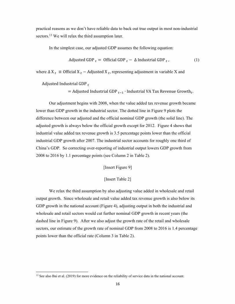
Our adjustment begins with 2008, when the value added tax revenue growth became

lower than GDP growth in the industrial sector. The dotted line in Figure 9 plots the

difference between our adjusted and the official nominal GDP growth (the solid line). The

adjusted growth is always below the official growth except for 2012. Figure 4 shows that

industrial value added tax revenue growth is 3.5 percentage points lower than the official

industrial GDP growth after 2007. The industrial sector accounts for roughly one third of

China’s GDP. So correcting over-reporting of industrial output lowers GDP growth from

2008 to 2016 by 1.1 percentage points (see Column 2 in Table 2).

[Insert Figure 9]

[Insert Table 2]

We relax the third assumption by also adjusting value added in wholesale and retail

output growth. Since wholesale and retail value added tax revenue growth is also below its

GDP growth in the national account (Figure 4), adjusting output in both the industrial and

wholesale and retail sectors would cut further nominal GDP growth in recent years (the

dashed line in Figure 9). After we also adjust the growth rate of the retail and wholesale

sectors, our estimate of the growth rate of nominal GDP from 2008 to 2016 is 1.4 percentage

points lower than the official rate (Column 3 in Table 2).

                                                            13 See also Bai et al. (2019) for more evidence on the reliability of service data in the national account.

17  

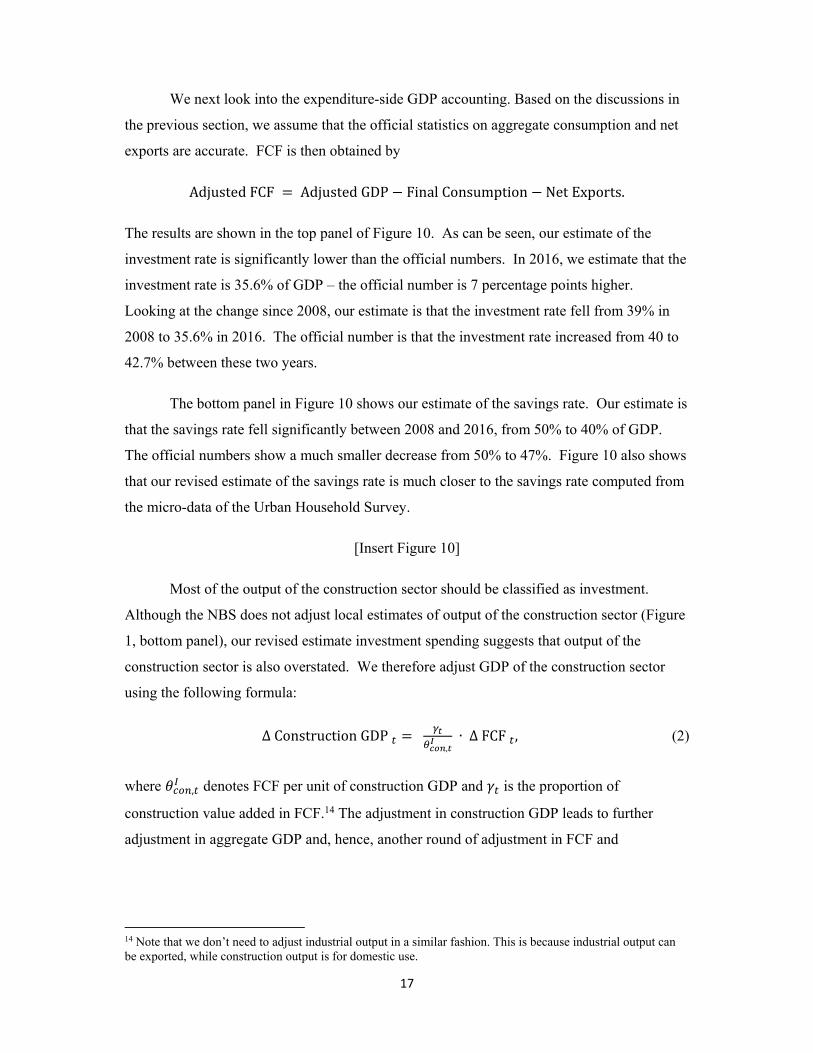
We next look into the expenditure-side GDP accounting. Based on the discussions in

the previous section, we assume that the official statistics on aggregate consumption and net

exports are accurate. FCF is then obtained by

AdjustedFCF AdjustedGDP FinalConsumption NetExports.

The results are shown in the top panel of Figure 10. As can be seen, our estimate of the

investment rate is significantly lower than the official numbers. In 2016, we estimate that the

investment rate is 35.6% of GDP – the official number is 7 percentage points higher.

Looking at the change since 2008, our estimate is that the investment rate fell from 39% in

2008 to 35.6% in 2016. The official number is that the investment rate increased from 40 to

42.7% between these two years.

The bottom panel in Figure 10 shows our estimate of the savings rate. Our estimate is

that the savings rate fell significantly between 2008 and 2016, from 50% to 40% of GDP.

The official numbers show a much smaller decrease from 50% to 47%. Figure 10 also shows

that our revised estimate of the savings rate is much closer to the savings rate computed from

the micro-data of the Urban Household Survey.

[Insert Figure 10]

Most of the output of the construction sector should be classified as investment.

Although the NBS does not adjust local estimates of output of the construction sector (Figure

1, bottom panel), our revised estimate investment spending suggests that output of the

construction sector is also overstated. We therefore adjust GDP of the construction sector

using the following formula:

∆ConstructionGDP , ∙ ∆FCF , (2)

where , denotes FCF per unit of construction GDP and is the proportion of

construction value added in FCF.14 The adjustment in construction GDP leads to further

adjustment in aggregate GDP and, hence, another round of adjustment in FCF and

                                                            14 Note that we don’t need to adjust industrial output in a similar fashion. This is because industrial output can be exported, while construction output is for domestic use.

18  

construction GDP. The full adjustment that balances aggregate GDP, construction GDP, and

FCF is given by:

AdjustedGDP OfficialGDP / ,

∆IndustrialGDP . (3)

Compared with (1), the GDP adjustment in (3) is amplified by adjusting construction output.

When we also adjust wholesale and retail GDP, ∆IndustrialGDP in (3) should be replaced

by ∆IndustrialGDP ∆WRGDP , where WR GDP denotes wholesale and retail GDP.

Column 4 in Table 2 reports the growth rate of nominal GDP after all three

adjustments (industrial, wholesale and retail trade, and construction output). With all three

adjustment, nominal GDP growth since 2013 is about half the official growth rate of nominal

GDP.15 Over the 2008-2016 period, our estimate of the GDP growth is 1.7 percentage points

lower than the official growth rate.

Section 3.2: Adjusting Local GDP

A similar procedure can be applied to correct provincial GDP. The published data on

revenues from value-added taxes do not break down revenues by province-industries.

However, value added tax revenues from industry, wholesale and retail account for more than

90% of total value added tax revenues before 2015 (see Figure A7 in the Appendix). We use

provincial value added tax revenue growth to proxy industrial, wholesale and retail value

added tax revenue growth in the province. The same benchmark adjustment for national GDP

can then be used for provincial GDP.16

[Insert Figure 11]

Figure 11 shows a scatterplot of our adjusted growth rate of provincial GDP against

the official growth rate of provincial GDP. The majority of the provinces lie below the 45

degree line, indicating that the official growth rate of most provinces exceeds our adjusted

estimates. The average difference is 1.4 percentage points. Guangdong and Zhejiang,

                                                            15 Figure A8 in the appendix plots the implied construction GDP growth. 16 We aggregate provincial GDP growth by our estimated provincial GDP, which is based on the estimated provincial GDP growth and uses 2007 official provincial GDP as the benchmark. We drop Shanghai and Beijing because they replaced the business tax with the value-added tax in 2012 and 2013, respectively. This change resulted in a 26% and 33% increase in revenues from value added taxes in the two years.

19  

however, are located on the 45 degree line.17 Among the provinces that are far below the 45

degree line are Liaoning (LN), Inner Mongolia (NM) and Tianjin (TJ). Local leaders in these

three provinces were recently arrested in corruption crackdowns, and one of the official

accusations was that these leaders had overstated local GDP. In addition, after the corruption

crackdown, the local statistical bureaus in Liaoning and Inner Mongolia issued new revised

estimates of local GDP in 2016 and 2017, respectively.18 The new numbers are 22% and

11% lower than the official numbers in the previous year. In comparison, our estimates show

that the unadjusted official GDP in Liaoning and Inner Mongolia is overstated by 17% and

20% in 2015, respectively. Furthermore, the official adjustment on industrial GDP accounts

for 70% of its adjustment on GDP in Liaoning. In the case of Inner Mongolia, the local

statistical bureau revised downwards its estimate of total value added of above-scale

industrial firms in 2016 by 290 billion Yuan, which accounts for the entire downward

revision in GDP of Inner Mongolia that year.

Adjusting local FCF is much harder. Unlike net exports at the national level that is

underpinned by custom data, provincial net outflows of goods and services are not based on

any data. Therefore, the adjustment for national FCF cannot be applied to provincial FCF.

We can however use the following equation to back out provincial FCF:

∑ , (4)

where is the province index, denotes the proportion of , sector ’s value added in

province , that is converted to fixed capital in province , denotes the net outflows of

sector ’s value added in province . The difficulty is, again, lack of data on .

We tackle the problem by using the IO table based on China’s value added tax

transaction-level records in 2017 (Bai, Luo and Song, 2019). While the data covers

essentially all the transactions among firms, the link between output and final use is missing.

Bearing in mind this limitation, we calculate the ratio of value added net outflows to total

value added for each sector and province pair and rewrite (4) as:

                                                            17 In private discussions, NBS officials indicated to us that Guangdong, Zhejiang, Beijing, and Shanghai are the four provinces with highest data quality. 18 While Tianjin acknowledged that the Binhai district overstated its GDP, it claimed that the district-level GDP overstatement didn’t affect Tianjin GDP.

20  

AdjustedFCF ∑ 1 ∙ AdjustedValueAdded . (5)

We then compare the adjusted provincial FCF with the official data in 2016 in Figure 12. We

find that most provinces over-report FCF and the extent of over-reporting is increasing in the

official investment rate. The over-reporting of FCF is most severe in western provinces such

as Ningxia and Qinghai. The FCF GDP ratio was overstated by more than 50 percentage

points in the two provinces. All the three provinces discussed earlier where local officials

“confessed” to manipulating local statistics are also associated with severe overstatement of

FCF. Their official FCF is about 40 to 50% higher than our estimates in 2015.19

[Insert Figure 12 and 13]

Figure 13 shows a positive correlation between the extent of over-reporting in

provincial GDP and that over-reporting in provincial FCF (the correlation is 0.61). While our

estimated provincial GDP and FCF are correlated by construction, there is no reason that the

adjustments to provincial GDP and FCF should be correlated. If measurement errors in

provincial GDP and FCF are large and independent, adjustments to the two variables would

be uncorrelated. Figure 14 thus provides evidence that local governments overstate both

GDP and FCF simultaneously

Section 3.3: Adjusting National Accounts with Statistical Models

A second approach is to explore the statistical relationship between GDP and a set of

economic indicators outside of China’s national accounts. We first estimate a model using the

provincial-level data prior to 2008 and then use the estimated model and the indicators to

predict provincial and national GDP after 2008. The success of the statistical approach

depends on three conditions. First, the indicators are informative about local economy and

unlikely to be manipulated. Second, local GDP growth data before 2008 is more reliable than

afterwards. Third, the statistical model is flexible enough to capture the rich heterogeneity

across Chinese provinces. We discuss the three conditions in order.

                                                            19 We use the 2014 FCF data for Liaoning because FCF in Liaoning declined by about 30% in 2015. Without a big adjustment in GDP, Liaoning’s net exports jumped from 104 billion Yuan in 2014 to 304 billion Yuan in 2015. In other words, before its GDP adjustment in 2016, Liaoning had scaled back its investment in 2015.

21  

Our indicators include satellite night lights, national tax revenue, exports and imports,

electricity consumption, railway cargo volume and new bank loans.20 National tax revenue is

collected by local government but directly paid to the central government. Cheating on

national tax revenue would incur fiscal losses and, hence, is unlikely to happen. Exports and

imports are from the custom data, which are hard to manipulate due to the symmetry of the

custom data from China’s trading partners. Electricity consumption, railway cargo volume

and new bank loans are from the so-called “Keqiang Index”, which Li Keqiang, China’s

current premier, used to monitor local economic performance when he was the Communist

Party Secretary of Liaoning province.

We understand the over-reporting of local GDP started in the late 1990s. So local

GDP growth data prior to 2008 cannot be entirely reliable. Yet, we also understand that GDP

over-reporting has become more severe since 2008. What we will identify from the following

exercise is the difference in the degree of GDP overstatement between the period prior to

2008 and the post-2008 period. Consequently, when we rely on local GDP growth data prior

to 2008, which is per se likely to be overstated, to estimate the subsequent growth, our

adjustment has to be a lower bound. The true GDP growth might be even lower than our

estimates for the post-2008 period.21

In terms of the statistical model, we will use the method developed by Su, Shi and

Phillips (2016) to control for hidden economic structure heterogeneities across regions.

Consider the following linear model:

,

where is log GDP of province at year , is a 1 vector of logarithm of the

indicators, is a 1 coefficient vector, captures provincial fixed effect and is the

i.i.d error term with mean zero. In the special case where , the model reduces to the

standard fixed effects regression. The more general model can capture heterogeneous

economic structures across regions. Intuitively, for the regions where local economy

heavily relies on resources might be very different from the others. Specifically, we assume

                                                            20 Using bank loans (not new bank loans) delivers similar results. 21 Our approach is fundamentally different from Fernald, Hsu and Spiegel (2015) and Clark, Pinkovskiy and Sala-i-Martin (2017), who use data on exports to China from its trading partners and night lights as independent measures of China’s economic activities. We instead train our statistical model by provincial industrial GDP data prior to 2007, when the overstatement of industrial GDP was much less evident compared to the post-2007 period.

22  

to be group-specific – i.e., , for all in group , where ∈ 1, 2, … , , ∈

1, 2, … , and . Instead of grouping provinces by geographical or economic

characteristics, we implement the classifier-Lasso (C-Lasso) method in Su, Shi and Phillips

(2016). The method provides statistical inference for membership identification, which is

totally data driven. We don’t have to rely on prior knowledge about the number of groups or

the number of provinces within each group. With the groups identified from C-Lasso, we can

use the fixed effects model to estimate the group-specific coefficients.

It is worth mentioning the rapid expansion of China’s service sector. According to the

national account data, service accounted for 43% of GDP in 2007 and the share increased to

52% in 2017. This is important because some of our indicators, like electricity consumption

and railway cargo volume, might be more relevant for industrial production than for service

production. If includes service output, the ongoing structural transformation would imply

time-varying and, hence, invalidate our model. To address the concern, we will use

provincial industrial GDP as in the benchmark and then use provincial GDP as a

robustness check. There are two reasons why we prefer provincial industrial GDP. First, the

stationarity of is more defensible for industrial GDP alone. Second, we have shown the

evidence that GDP overstatement is larger in the industrial sector.

Our sample consists of annual observations from 30 provinces (excluding Tibet)

between 2000 and 2017. GDP, electricity consumption, exports and imports, railway cargo

volume and new bank loans are all from NBS; national tax revenue is from China Taxation

Yearbook; we use the DMSP-OLS night time lights data from National Oceanic and

Atmospheric Administration (NOAA) in the United States.22 The time series are shorter for

some variables. Satellite night lights data ends at 2013. National tax revenue data ends at

2015 because the reform “to replace business tax with value-added tax” made national tax

revenue not comparable before and after 2016.

Two remarks are in order. First, night lights data, electricity consumption and railway

freight are all in real terms. As a robustness check, we use GDP deflators to convert GDP,

national tax revenue, exports and imports and bank loans into real terms in the regressions

(see also Clark et al., 2017). The estimated GDP will be converted back into nominal terms.

The technical appendix reports the results with price adjustments. The differences are small.

                                                            22 The night light data is not comparable before and after 2010 due to the satellite change. We use the average of the light growth in 2009 and 2011 to proxy the 2010 light growth for out-of-sample predictions.

23  

Second, we can use more data in the earlier period to estimate the model, with a caveat that

the estimated model might be less applicable to the recent years due to structural changes. In

the Appendix, we estimate the model by the data between 1995 (the year after

implementation of the tax sharing reform) and 2007. The main results are very similar.

We first apply LASSO to the 2000-2007 data for model selection. K-fold cross

validation, EBIC (Extended Bayesian Information Criterion) and data-driven penalty with

heteroscedasticity (Belloni et al., 2012, 2014, 2016) suggest to keep all the indicators except

for new bank loans. Besides the statistical evidence, there is also an economic reason for us to

drop bank loans. The “fiscal stimulus” launched by the Chinese government in the late 2008

relaxed the borrowing constraint on local governments and led to a debt explosion afterwards

(Bai, Song and Hsieh, 2016). Much of the fund raised by local government financing vehicles

is believed to finance infrastructure investment, rather than production. This implies a

structural change in the way that new bank loans contribute to GDP.

Our estimation is done in three steps. First, using the sample prior to 2008, we run the

C-Lasso estimation and to classify provinces into different groups. Second, we estimate

group-specific coefficients by post-Lasso OLS regressions. Finally, the estimated and the

same set of the indictors are used to estimate provincial secondary industry value added

throughout the whole sample period. Assuming provincial agriculture, construction and

service GDP are reliable, we can estimate provincial GDP, which will be added to obtain

aggregate GDP. Note that the estimated industrial value added after 2008 is out-of-sample

prediction, while the estimation before 2008 is in-sample prediction.

When we use provincial industrial GDP, the C-Lasso procedure doesn’t find statistical

evidence for grouping, suggesting that the relationship between industrial GDP and these

indicators is similar across provinces. As will be seen below, the result would be different if

we replace provincial industrial GDP with provincial GDP. Since the satellite night lights

data is not available after 2013, it can only be used for the out-of-sample prediction between

2008 and 2013. We re-run the C-Lasso and post-Lasso OLS regressions without night lights.

The estimated model can make out-of-sample predictions for the post-2013 period.23

The out-of-sample predictions are shown in Figure 14 and Table 2. While the in-

sample predictions are close to the official numbers, the out-of-sample predictions are more

                                                            23 The tables with the regression coefficients are the appendix.

24  

volatile and lower than the official numbers in recent years. The estimated GDP growth is

about 0.5 to 1 percentage points lower than the official GDP growth in 2014 and 2016 (see

the solid and dotted line in Figure 14 and Column 5 and 6 in Table 2).

[Insert Figure 14]

We note that although our two approaches are fundamentally different, they yield

similar results in terms of the magnitude of overstatement of GDP. Table 2 shows that

nominal GDP growth was overstated after 2008 and more so after 2013, and the magnitude of

the overstatement after 2013 was about one to two percentage points.

One may wonder to what extent tax revenue data used by the two approaches can

explain their similar results on the recent over-reporting of GDP. First to notice is that tax

revenue data are not identical in the two approaches. The first approach uses value added tax

revenue, while the second approach uses national tax revenue, which includes but is not

limited to consumption tax, part of value added and corporate income tax revenue. Still, it

would be interesting to see how the estimated GDP would look like from the second

approach without tax revenue data. To this end, we re-run the regressions without national tax

revenue. Another advantage of dropping national tax revenue is to extend the estimation to

the whole sample period. The results are shown in Figure 14 and the last column in Table 2.

The overstatement in GDP growth after 2013 appears to be a robust finding, though its

magnitude does depend on estimation method and variable selection.

Panel A of Figure 15 plots the extent of GDP overstatement across provinces

estimated by the first approach and the second approach with national tax revenue. Since the

second approach only adjust industrial GDP, we use the first approach that adjusts industrial

GDP only to make the two approaches more comparable. The correlation is 0.62. Panel B

uses the estimates by the second approach without national tax revenue. Encouragingly, they

are still positively correlated, with a correlation of 0.38. In other words, the different methods

using independent data sources deliver positively correlated estimates on provincial GDP

overstatement.

[Insert Figure 15]

We next replace provincial industrial GDP with provincial GDP for robustness check.

We drop both railway cargo volume and new bank loans as suggested by LASSO. Given the

huge disparity in GDP composition across provinces, not surprisingly, C-Lasso identifies two

25  

groups, with 14 provinces in Group 1 and 16 provinces in Group 2. See Appendix II for the

detailed grouping results. Interestingly, Beijing, Shanghai and Hainan, the three provinces

with the highest service GDP share, are all in Group 1. The fixed effects regression results for

each group are reported in the appendix. Coefficients are indeed quite different across groups.

We then run C-Lasso without light data, which also identifies two groups, with 11 and 19

provinces in Group 1 and 2. Appendix II shows that 10 out of 11 provinces in Group 1 are in

Group 1 identified by C-Lasso with light data. Again, Beijing, Shanghai and Hainan are all in

Group 1.

Figure 16 compares the GDP growth rates from the official data, our estimates using

provincial industrial GDP, provincial GDP with light data, provincial GDP without light data,

and provincial GDP without light or tax data. Estimating provincial GDP directly implies

much bigger GDP overstatement. The difference between the official GDP growth and our

estimate is more than five percentage points in 2015. As discussed above, the caveat is the

misspecification of the model that fails to capture how the rise of the service sector affects

GDP growth.

[Insert Figure 16]

 

4. Other Implications

We summarize here the three main implications of our results. First, nominal GDP

growth after 2008 and particularly after 2013 is lower than suggested by the official statistics.

Second, the savings rate has declined by 10 percentage points between 2008 and 2016. The

official statistics suggest the savings rate only declined by 3 percentage points between these

two years. Third, our statistics suggest that the investment rate has fell by about 3% of GDP

between 2008 and 2016. Official statistics suggest that the investment rate has increased over

this period.

We note that we do not have independent information on GDP deflators so our

statement is only about nominal GDP growth. The literature has questioned the reliability of

China’s official price indices, but we do not have independent information on the deflators.24

                                                            24 See, for example, Brandt and Zhu (2010) and Nakamura, Steinsson and Liu (2016).

26  

Keep in mind the caveats, we think it is useful to convert nominal output and input into real

terms using the official GDP deflators and investment goods price index.

For real GDP growth, we calculate real GDP in the industrial, construction, wholesale

and retail sectors using our estimated nominal GDP (first approach) and the official GDP

deflators for the three sectors. Adding adjusted real GDP in the three sectors to real GDP in the

other sectors gives our adjusted real GDP shown in Figure 17. On average, the annual real GDP

growth was overstated by 2 percentage points between 2008 and 2016. The official real GDP

is 16% above our estimate in 2016.

[Insert Figure 17]

We now discuss the implications of our findings for capital returns, TFP growth, and

the debt to GDP ratio. We begin with the return to capital. We use the following equation to

estimate returns to capital:

α/

δ ,

where denotes real returns to capital, denotes nominal returns to capital, denotes the

growth rate of output price, denotes the growth rate of capital goods price, α denotes the

share of capital income in output, / denotes the nominal capital-output ratio and δ is

the depreciation rate.

The results are plotted in Figure 18.25 The solid line uses the official data and

replicates the earlier estimates in Bai et al. (2006) and the more recent ones in Bai and Zhang

(2015). Recall that our adjustment of production GDP also lowers investment which

increases the ratio of output to capital. While our estimated capital returns are about one to

two percentage points higher than those using official data, the dramatic decline in aggregate

returns to capital in the post-2007 period turns out to be a robust phenomenon.

[Insert Figure 18]

To estimate TFP, we assume the following aggregate production function:

,

                                                            25 We discuss the details of the data used to estimate the return to capital in the appendix.

27  

where is real GDP, is aggregate TFP, is real capital, is human capital per worker and

is the number of workers.26 The results are plotted in Figure 19. The aggregate TFP growth

rates by our estimates appear to be more volatile than those by official data. Yet, it remains

obvious that China’s aggregate TFP growth slowed down substantially after 2007.

[Insert Figure 19]

Finally, Figure 20 shows the debt to GDP ratio with our revised estimate of nominal

GDP. The estimation of debt follows Song and Xiong (2018). The bottom line is that our

revised numbers suggest that the debt to GDP ratio has increased by more than suggested by

the official numbers. Our estimate of the debt to GDP ratio in 2016 is 2.4 – the official

number is 2.1.

[Insert Figure 20]

 

5. Conclusion

The broader point is that the collection of data behind the national accounts is under

the control of local governments. This is not surprising, as many administrative functions are

controlled by powerful local governments. In Bai, Hsieh and Song (2019), we argue that

local governments have used this power to support a large number of private businesses. The

question in this paper is what local governments choose to do with their power over local

statistics.

We document that local governments have chosen to use their power to inflate local

statistics on GDP, particularly by overstating industrial output and investment. As evidence,

we show that the sum of local GDP has exceeded aggregate GDP since 2003. One possible

explanation for why they do this is the introduction of local economic performance in the

evaluation of local officials by the Chinese Communist Party’s Organization Department in

                                                            26 We set 0.5 (the results are similar if we use time-varying calibrated in the appendix for estimating returns to capital). We assume ⋅ , where is the year of schooling and is the return to schooling. The average year of schooling for workers in 2000 and 2005 is from the 2000 census and 2005 one-percent population survey data. We obtain the numbers between 2001 and 2004 by linear interpolation. For 2006 to 2016, we use the numbers from the labour force survey in the Statistical Yearbooks of Population and Employment. For 1990 to 1999, we assume the annual growth of to be its average average growth in 2000-2005. We then use the 2005 one-percent population survey data to estimate returns to education by the Mincer earnings regression, which gives 0.126.

28  

the late 1990s. The official documentation of this policy change states that local officials will

be evaluated based on “the speed, efficiency and potentials of economic development, the

growth of fiscal revenue, the improvement of people’s living standards.” (Provisional

Regulations on Evaluating Party and Government Cadres, Central Organization Department

of China’s Communist Party, 1998). The revision intensified economic competition between

local governments, and it seems likely that many local governments resorted to inflating local

GDP numbers. Xiong (2018) provides a theoretical framework where competition between

local governments results in both overstatement of GDP as well as investment. And Lyu et

al. (2018) present evidence that regional growth target can be achieved by fabricating data.

The possibility that local governments misreport local GDP is well known, and the

Central Government’s National Bureau of Statistics adjusts the numbers reported by local

governments. Prior to 2003, the NBS adjusted upwards local GDP but after 2003, the NBS

adjusted local GDP downwards. However, our estimates suggest that the extent by which

local governments exaggerate local GDP accelerated after 2008, but the magnitude of the

adjustment by the NBS did not change in tandem. As a consequence, our best estimate is that

the true growth rate of GDP is probably overstated by almost 2 percentage points from 2008

to 2016.

A final question is what tools and what incentive does the NBS have to report

accurate statistics. We document that much of the underlying data behind the national

accounts is out of the hands of the NBS. Furthermore, the question is what incentives does

the NBS has to resist local officials who misreport data. Interestingly, although the NBS

adjusts downwards local statistics, it does not report the adjusted local statistics, perhaps out

of a desire to not confront powerful local leaders. Given the weak position of the NBS and

the strong position of local leaders in the Chinese political system, it is not surprising that

statistical data are potentially biased.

29  

References

Bai, Chong-En, Chang-Tai Hsieh, and Yingyi Qian. 2006. "The Return to Capital in China." Brookings Papers on Economic Activity, Fall: 61-101.

Bai, Chong-En, Chang-Tai Hsieh, and Zheng Song. 2016. "The Long Shadow of China's Fiscal Expansion." Brookings Papers on Economic Activity, Fall: 129-181.

Bai, Chong-En, Chang-Tai Hsieh, and Zheng Song. 2019. "Special Deals with Chinese Characteristics." NBER Macroeconomics Annual, forthcoming.

Bai, Chong-En, Xilu Chen, Zheng Song, and Xin Wang. 2019. "The Rise of China's Service Sector." Working Paper.

Bai, Chong-En, Jie Luo and Zheng Song. 2019. "China's Input-Output Table from Value Added Tax Invoices." Working Paper.

Bai, Chong-En, and Qiong Zhang. 2015. "The Return on Capital in China and Its Determinants." China Economist 10, no. 3: 20-37.

Brandt, Loren, and Xiaodong Zhu. 2010. "Accounting for China's Growth." Working Paper.

Central Organization Department of China’s Communist Party. 1998. "Provisional Regulations on Evaluating Party and Government Cadres" [in Chinese]. Document no. 6, May 26. http://cpc.people.com.cn/GB/64162/71380/71382/71480/ 4853966.html

Clark, Hunter, Maxim Pinkovskiy, and Xavier Sala-i-Martin. 2017. "China's GDP Growth May Be Understated." Working Paper no. 23323. Cambridge, Mass.: National Bureau of Economic Research.

Fernald, John G., Eric Hsu, and Mark M. Spiegel. 2015. "Is China Fudging Its Figures? Evidence from Trading Partner Data." Working Paper.

Gao, Jie. 2016. "Bypass the Lying Mouths: How Does the CCP Tackle Information Distortion at Local Levels?" The China Quarterly 228: 950-969.

Holz, Carsten A. 2013. "Chinese Statistics: Output Data." Working Paper.

Holz, Carsten A. 2014. "The Quality of China's GDP Statistics." China Economic Review 30: 309-338.

Holz, Carsten A. 2015. "China's Investment Rate: Implications and Data Reliability." Working Paper.

Holz, Carsten A., and Yue Sun. 2018. "Physical Capital Estimates for China's Provinces, 1952–2015 and Beyond." China Economic Review 51: 342-357.

Lei, Yu-Hsiang. 2017. "Quid Pro Quo? Government-Firm Relationships in China. " Working Paper.

Liu, Fang, Jun Zhang, and Tian Zhu. 2016. "How Much Can We Trust China’s Investment Statistics?" Journal of Chinese Economic and Business Studies 14, no. 3: 215-228.

30  

Lyu, Changjiang, Kemin Wang, Frank Zhang, and Xin Zhang. 2018. "GDP Management to Meet or Beat Growth Targets." Journal of Accounting and Economics 66, no. 1: 318-338.

Ma, Ben, Guojun Song, Lei Zhang, and David A. Sonnenfeld. 2014. "Explaining Sectoral Discrepancies between National and Provincial Statistics in China." China Economic Review 30: 353-369.

Nakamura, Emi, Jón Steinsson, and Miao Liu. 2016. "Are Chinese Growth and Inflation Too Smooth? Evidence from Engel Curves." American Economic Journal: Macroeconomics 8, no. 3: 113-144.

Orlik, Tom. 2014. "Reform at China's National Bureau of Statistics under Ma Jiantang 2008-2013." China Economic Review 30: 304-308.

Song, Zheng, and Wei Xiong. 2018. "Risks in China's Financial System." Annual Review of Financial Economics 10: 261-286.

Su, Liangjun, Zhentao Shi, and Peter C. B. Phillips. 2016. "Identifying Latent Structures in Panel Data." Econometrica 84, no. 6: 2215-2264.

Wang, Xiaolu, and Lian Meng. 2001. "A Reevaluation of China's Economic Growth. " China Economic Review 12, no. 4, 338-346.

Xiong, Wei. 2018. "The Mandarin Model of Growth." Working Paper no. 25296. Cambridge, Mass.: National Bureau of Economic Research.

Xu, Xianchun. 2004. "China's Gross Domestic Product Estimation." China Economic Review 15, no. 3: 302-322.

Xu, Xianchun. 2014. "Accurate Understanding of China's Income, Consumption and Investment." Social Sciences in China 35, no. 1: 21-43.

Xu, Yan. 2011. "Reforming Value Added Tax in Mainland China: A Comparison with the EU." Revenue Law Journal 20, no. 1, article 4.

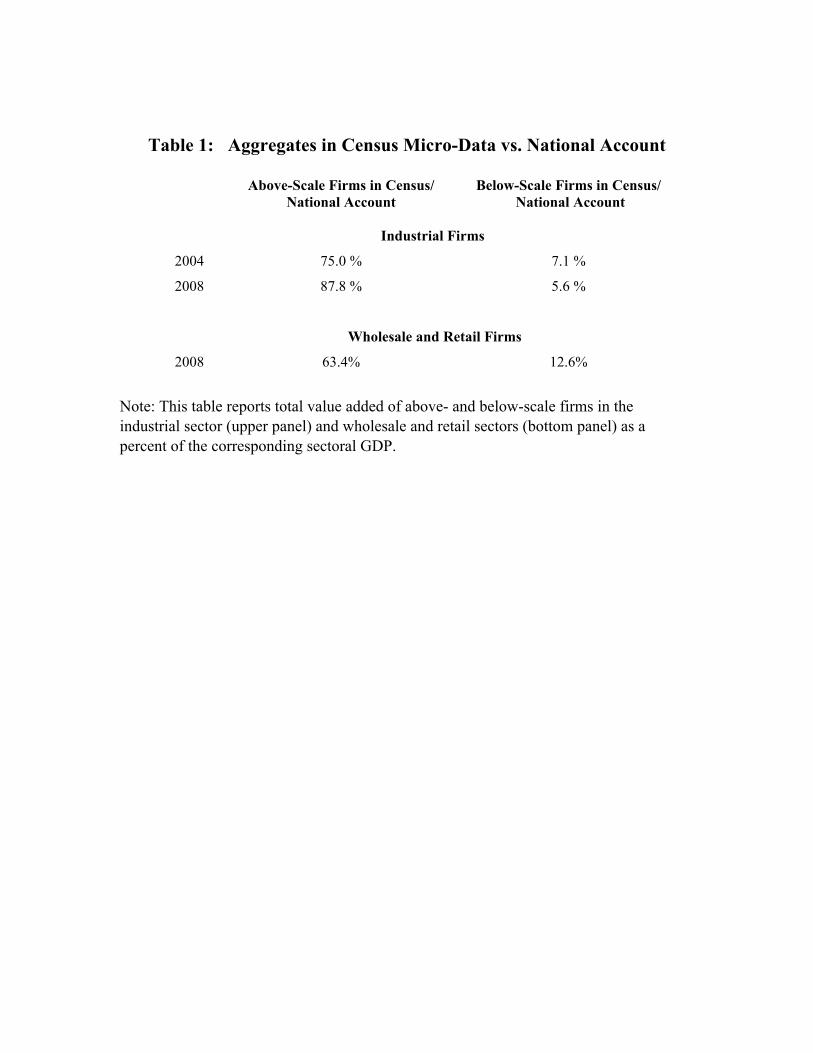
Table 1: Aggregates in Census Micro-Data vs. National Account

Above-Scale Firms in Census/ National Account

Below-Scale Firms in Census/ National Account

Industrial Firms

2004 75.0 % 7.1 %

2008 87.8 % 5.6 %

Wholesale and Retail Firms

2008 63.4% 12.6%

Note: This table reports total value added of above- and below-scale firms in the industrial sector (upper panel) and wholesale and retail sectors (bottom panel) as a percent of the corresponding sectoral GDP.

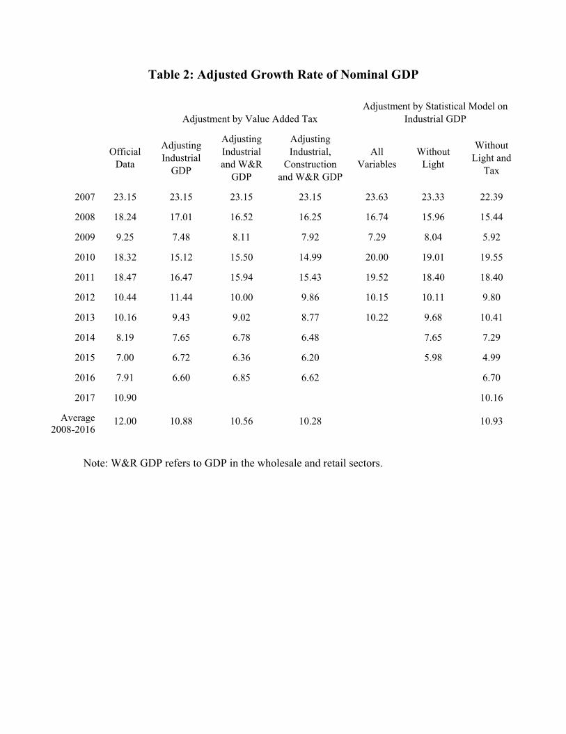
Table 2: Adjusted Growth Rate of Nominal GDP

Adjustment by Value Added Tax

Adjustment by Statistical Model on Industrial GDP

Official Data

Adjusting Industrial

GDP

Adjusting Industrial and W&R

GDP

Adjusting Industrial,

Construction and W&R GDP

All Variables

Without Light

Without Light and

Tax

2007 23.15 23.15 23.15 23.15 23.63 23.33 22.39

2008 18.24 17.01 16.52 16.25 16.74 15.96 15.44

2009 9.25 7.48 8.11 7.92 7.29 8.04 5.92

2010 18.32 15.12 15.50 14.99 20.00 19.01 19.55

2011 18.47 16.47 15.94 15.43 19.52 18.40 18.40

2012 10.44 11.44 10.00 9.86 10.15 10.11 9.80

2013 10.16 9.43 9.02 8.77 10.22 9.68 10.41

2014 8.19 7.65 6.78 6.48

7.65 7.29

2015 7.00 6.72 6.36 6.20 5.98 4.99

2016 7.91 6.60 6.85 6.62

6.70

2017 10.90

10.16

Average 2008-2016

12.00 10.88 10.56 10.28 10.93

Note: W&R GDP refers to GDP in the wholesale and retail sectors.

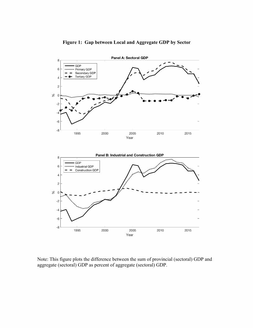
Figure 1: Gap between Local and Aggregate GDP by Sector

Note: This figure plots the difference between the sum of provincial (sectoral) GDP and aggregate (sectoral) GDP as percent of aggregate (sectoral) GDP.

   

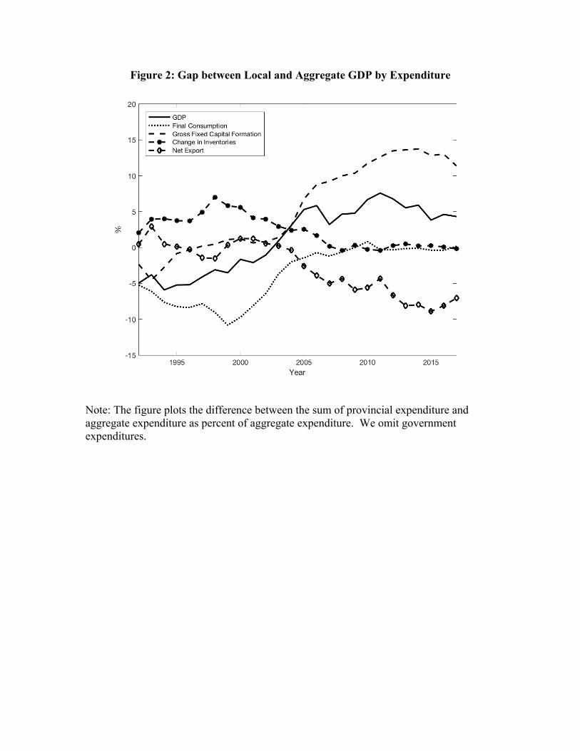
Figure 2: Gap between Local and Aggregate GDP by Expenditure

Note: The figure plots the difference between the sum of provincial expenditure and aggregate expenditure as percent of aggregate expenditure. We omit government expenditures.

   

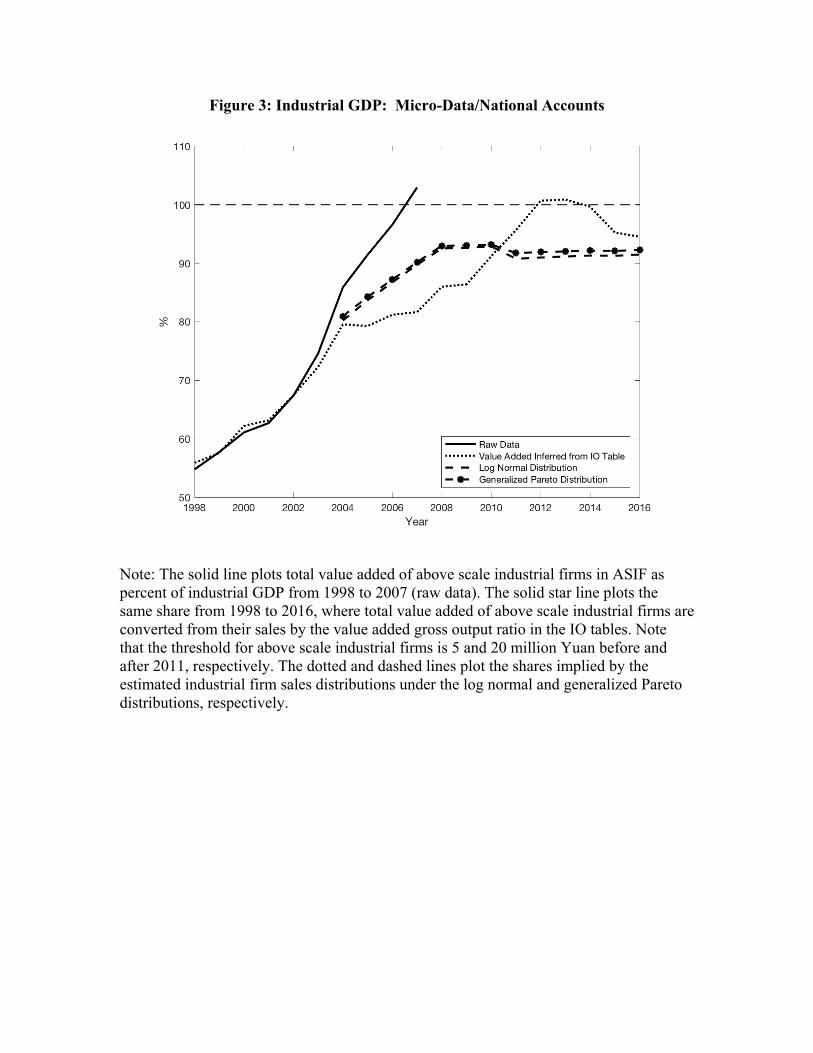
Figure 3: Industrial GDP: Micro-Data/National Accounts

Note: The solid line plots total value added of above scale industrial firms in ASIF as percent of industrial GDP from 1998 to 2007 (raw data). The solid star line plots the same share from 1998 to 2016, where total value added of above scale industrial firms are converted from their sales by the value added gross output ratio in the IO tables. Note that the threshold for above scale industrial firms is 5 and 20 million Yuan before and after 2011, respectively. The dotted and dashed lines plot the shares implied by the estimated industrial firm sales distributions under the log normal and generalized Pareto distributions, respectively.

   

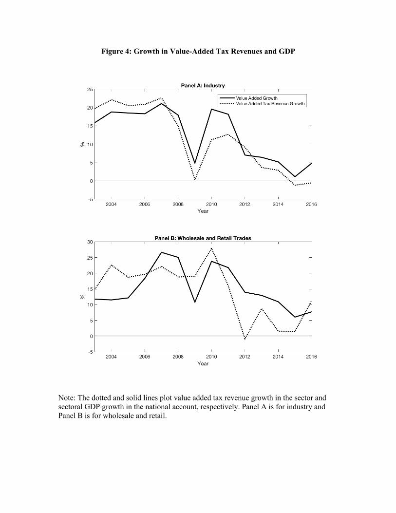
Figure 4: Growth in Value-Added Tax Revenues and GDP

Note: The dotted and solid lines plot value added tax revenue growth in the sector and sectoral GDP growth in the national account, respectively. Panel A is for industry and Panel B is for wholesale and retail.    

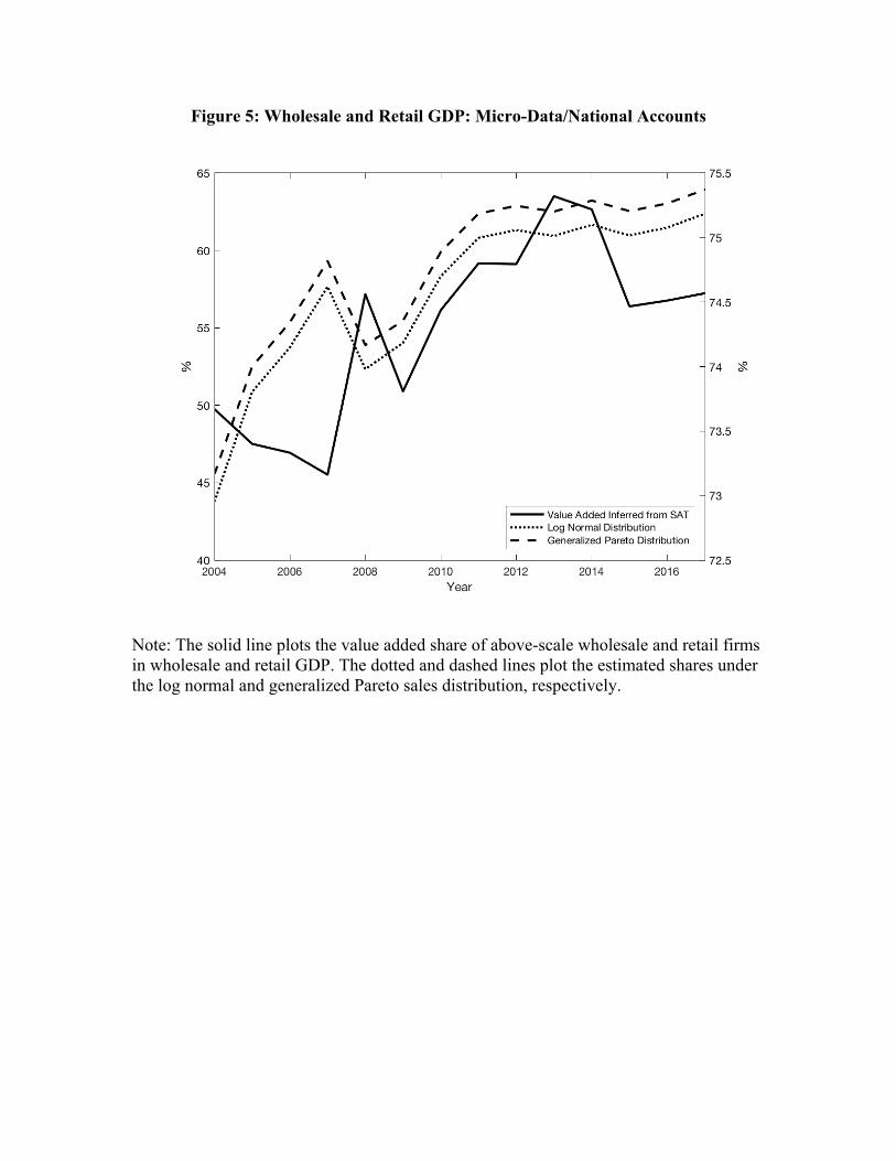
Figure 5: Wholesale and Retail GDP: Micro-Data/National Accounts

Note: The solid line plots the value added share of above-scale wholesale and retail firms in wholesale and retail GDP. The dotted and dashed lines plot the estimated shares under the log normal and generalized Pareto sales distribution, respectively.

   

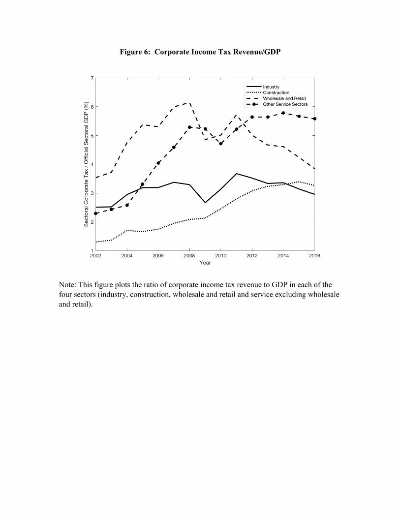
Figure 6: Corporate Income Tax Revenue/GDP

Note: This figure plots the ratio of corporate income tax revenue to GDP in each of the four sectors (industry, construction, wholesale and retail and service excluding wholesale and retail).

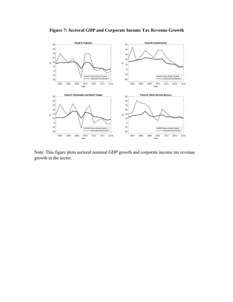
Figure 7: Sectoral GDP and Corporate Income Tax Revenue Growth

Note: This figure plots sectoral nominal GDP growth and corporate income tax revenue growth in the sector.

   

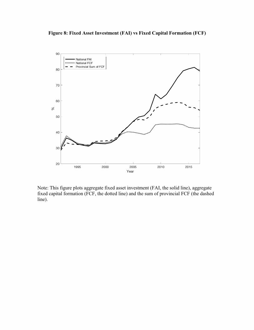
Figure 8: Fixed Asset Investment (FAI) vs Fixed Capital Formation (FCF)

Note: This figure plots aggregate fixed asset investment (FAI, the solid line), aggregate fixed capital formation (FCF, the dotted line) and the sum of provincial FCF (the dashed line).

   

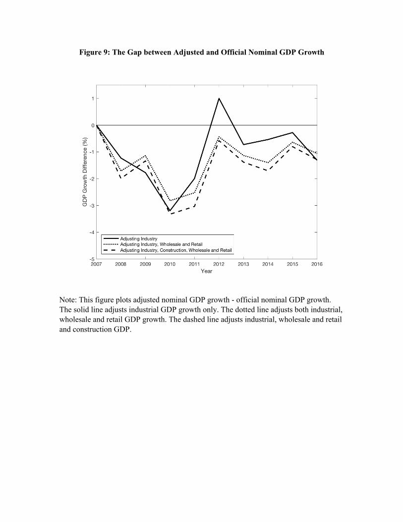
Figure 9: The Gap between Adjusted and Official Nominal GDP Growth

Note: This figure plots adjusted nominal GDP growth - official nominal GDP growth. The solid line adjusts industrial GDP growth only. The dotted line adjusts both industrial, wholesale and retail GDP growth. The dashed line adjusts industrial, wholesale and retail and construction GDP.

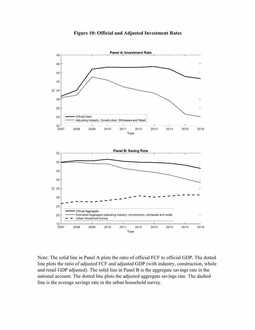
Figure 10: Official and Adjusted Investment Rates

Note: The solid line in Panel A plots the ratio of official FCF to official GDP. The dotted line plots the ratio of adjusted FCF and adjusted GDP (with industry, construction, whole and retail GDP adjusted). The solid line in Panel B is the aggregate savings rate in the national account. The dotted line plots the adjusted aggregate savings rate. The dashed line is the average savings rate in the urban household survey.

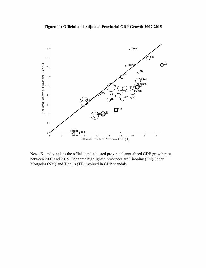
Figure 11: Official and Adjusted Provincial GDP Growth 2007-2015

Note: X- and y-axis is the official and adjusted provincial annualized GDP growth rate between 2007 and 2015. The three highlighted provinces are Liaoning (LN), Inner Mongolia (NM) and Tianjin (TJ) involved in GDP scandals.

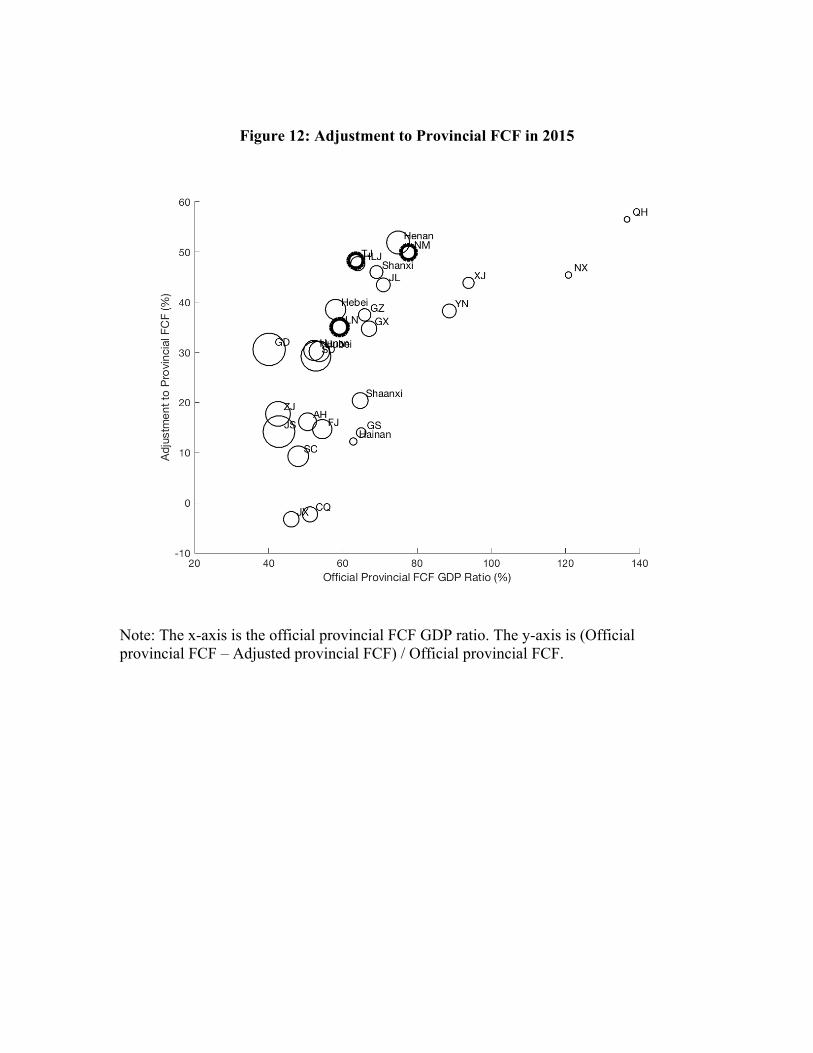
Figure 12: Adjustment to Provincial FCF in 2015

Note: The x-axis is the official provincial FCF GDP ratio. The y-axis is (Official provincial FCF – Adjusted provincial FCF) / Official provincial FCF.

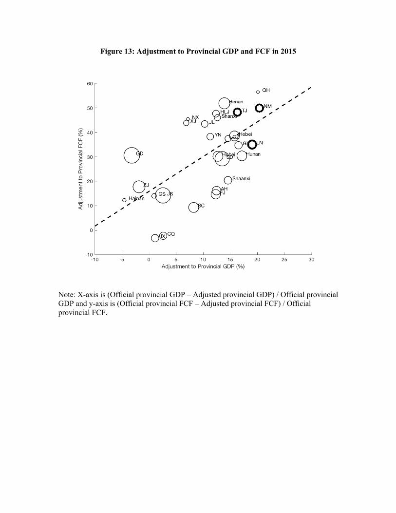
Figure 13: Adjustment to Provincial GDP and FCF in 2015

Note: X-axis is (Official provincial GDP – Adjusted provincial GDP) / Official provincial GDP and y-axis is (Official provincial FCF – Adjusted provincial FCF) / Official provincial FCF.

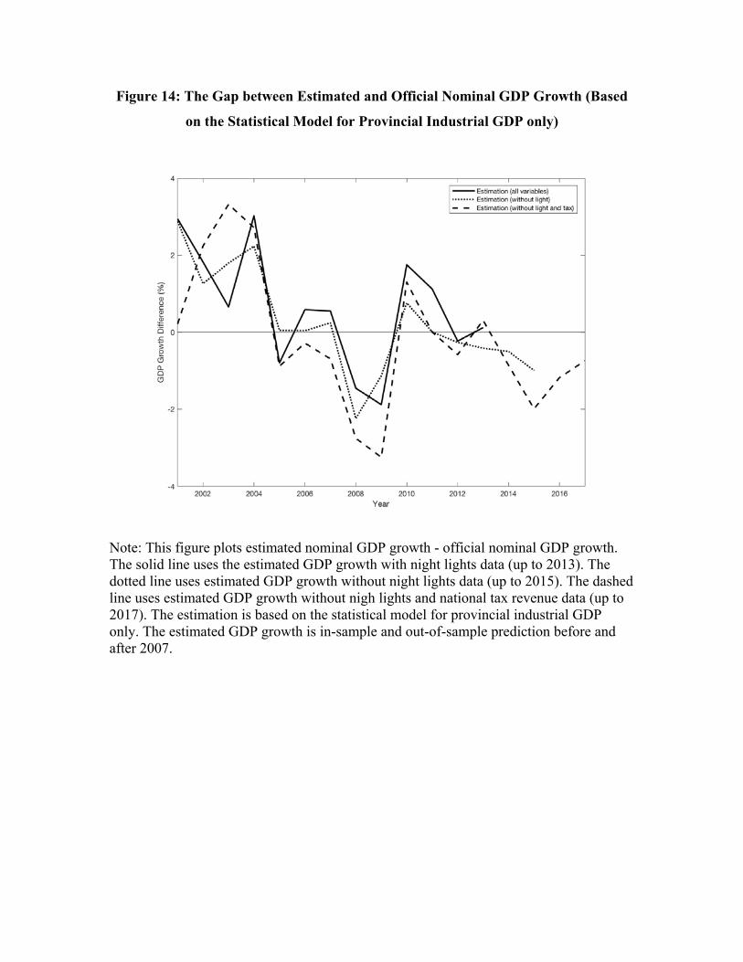
Figure 14: The Gap between Estimated and Official Nominal GDP Growth (Based

on the Statistical Model for Provincial Industrial GDP only)

 

Note: This figure plots estimated nominal GDP growth - official nominal GDP growth. The solid line uses the estimated GDP growth with night lights data (up to 2013). The dotted line uses estimated GDP growth without night lights data (up to 2015). The dashed line uses estimated GDP growth without nigh lights and national tax revenue data (up to 2017). The estimation is based on the statistical model for provincial industrial GDP only. The estimated GDP growth is in-sample and out-of-sample prediction before and after 2007.

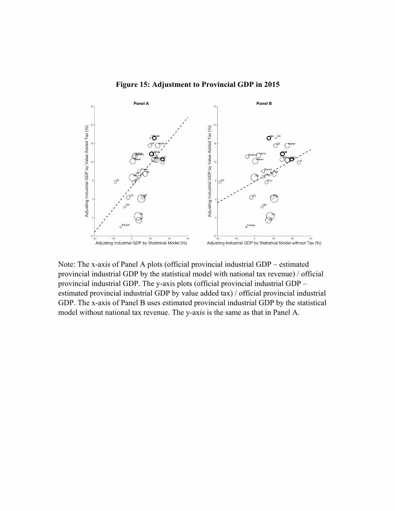
Figure 15: Adjustment to Provincial GDP in 2015

Note: The x-axis of Panel A plots (official provincial industrial GDP – estimated provincial industrial GDP by the statistical model with national tax revenue) / official provincial industrial GDP. The y-axis plots (official provincial industrial GDP – estimated provincial industrial GDP by value added tax) / official provincial industrial GDP. The x-axis of Panel B uses estimated provincial industrial GDP by the statistical model without national tax revenue. The y-axis is the same as that in Panel A.

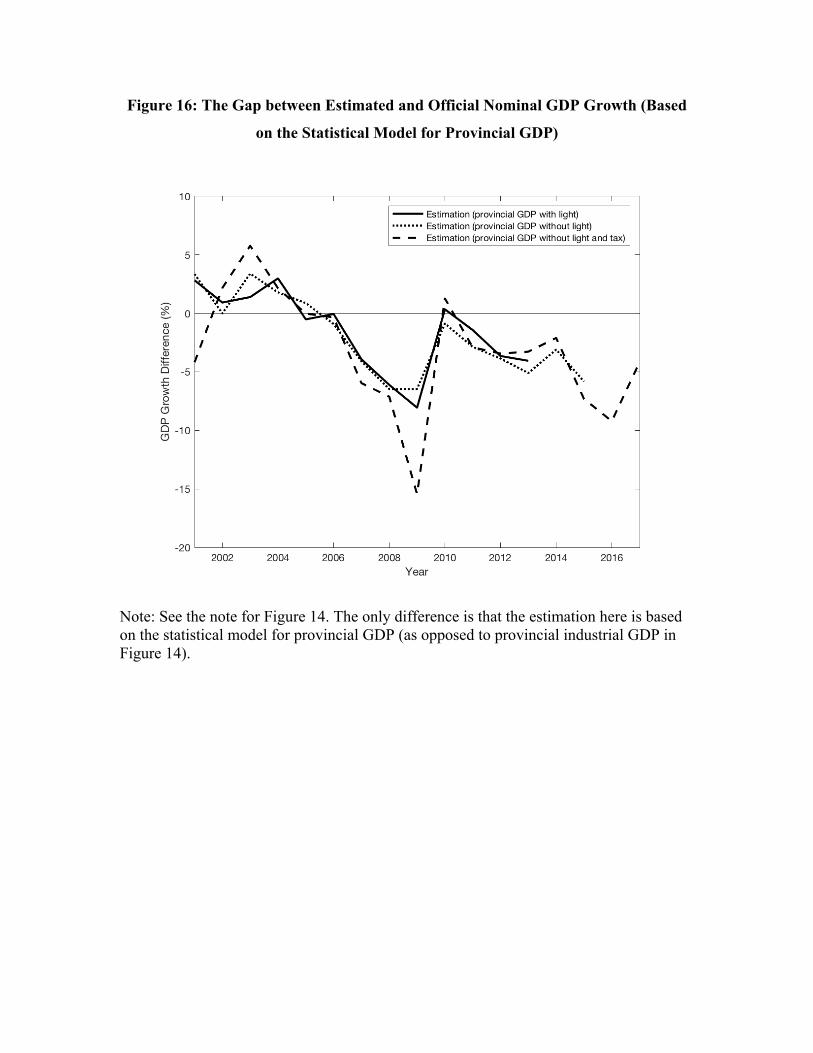
Figure 16: The Gap between Estimated and Official Nominal GDP Growth (Based

on the Statistical Model for Provincial GDP)

Note: See the note for Figure 14. The only difference is that the estimation here is based on the statistical model for provincial GDP (as opposed to provincial industrial GDP in Figure 14).

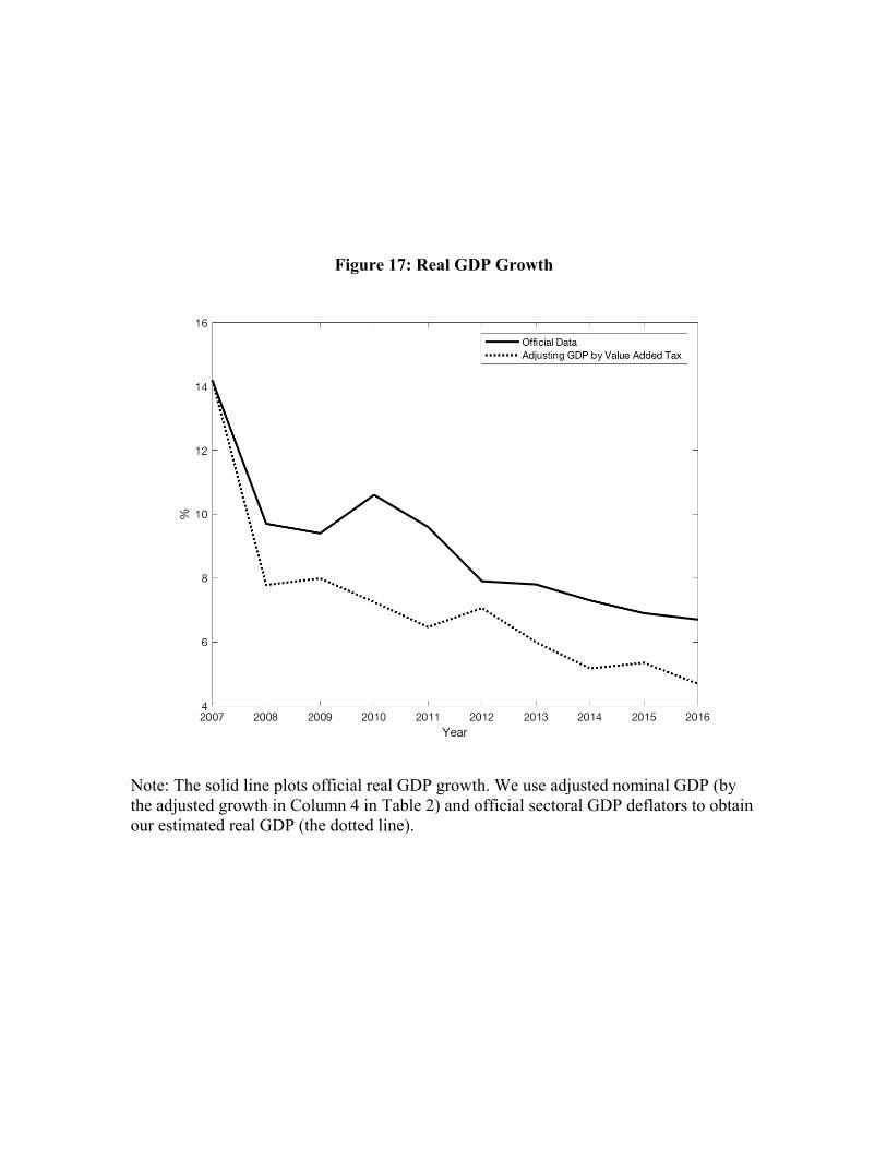
Figure 17: Real GDP Growth

Note: The solid line plots official real GDP growth. We use adjusted nominal GDP (by the adjusted growth in Column 4 in Table 2) and official sectoral GDP deflators to obtain our estimated real GDP (the dotted line).

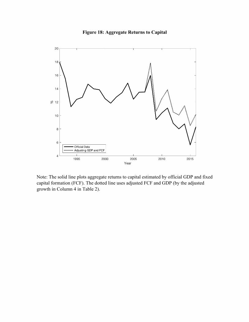
Figure 18: Aggregate Returns to Capital

Note: The solid line plots aggregate returns to capital estimated by official GDP and fixed capital formation (FCF). The dotted line uses adjusted FCF and GDP (by the adjusted growth in Column 4 in Table 2).

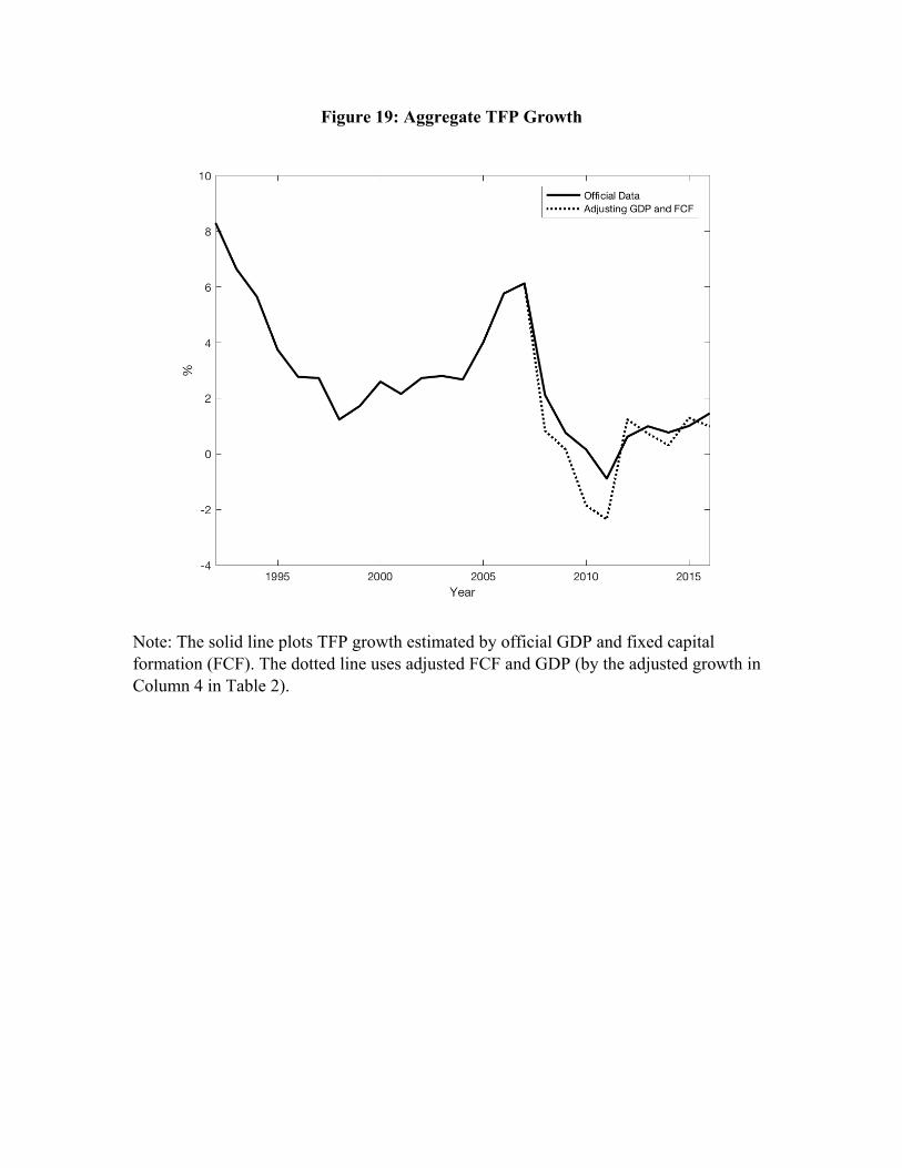
Figure 19: Aggregate TFP Growth

Note: The solid line plots TFP growth estimated by official GDP and fixed capital formation (FCF). The dotted line uses adjusted FCF and GDP (by the adjusted growth in Column 4 in Table 2).

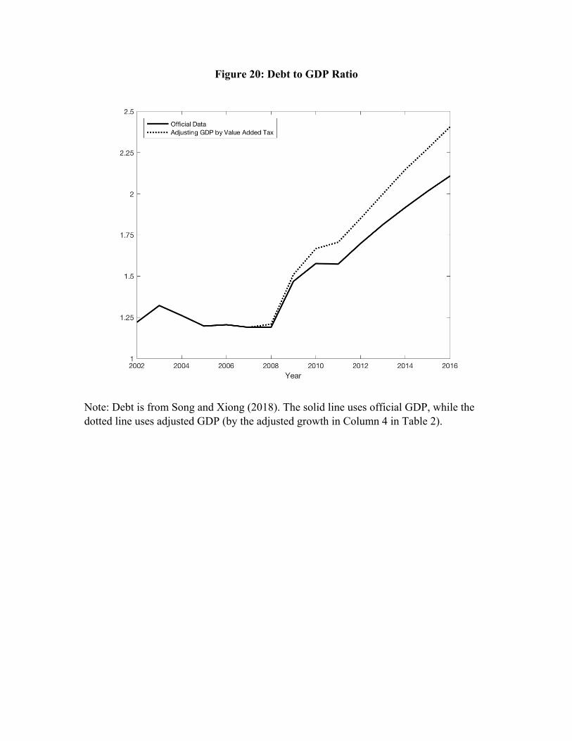
Figure 20: Debt to GDP Ratio

Note: Debt is from Song and Xiong (2018). The solid line uses official GDP, while the dotted line uses adjusted GDP (by the adjusted growth in Column 4 in Table 2).