Embed Size (px)
Citation preview

The University of Manchester Research
A Food-Energy-Water Nexus approach for land useoptimizationDOI:10.1016/j.scitotenv.2018.12.242
Document VersionAccepted author manuscript
Link to publication record in Manchester Research Explorer
Citation for published version (APA):Nie, Y., Avraamidou, S., Xiao, X., Pistikopoulos, E. N., Li, J., Zeng, Y., Song, F., Yu, J., & Zhu, M. (2019). A Food-Energy-Water Nexus approach for land use optimization. Science of the Total Environment, 659, 7-19.https://doi.org/10.1016/j.scitotenv.2018.12.242
Published in:Science of the Total Environment
Citing this paperPlease note that where the full-text provided on Manchester Research Explorer is the Author Accepted Manuscriptor Proof version this may differ from the final Published version. If citing, it is advised that you check and use thepublisher's definitive version.
General rightsCopyright and moral rights for the publications made accessible in the Research Explorer are retained by theauthors and/or other copyright owners and it is a condition of accessing publications that users recognise andabide by the legal requirements associated with these rights.
Takedown policyIf you believe that this document breaches copyright please refer to the University of Manchester’s TakedownProcedures [http://man.ac.uk/04Y6Bo] or contact [email protected] providingrelevant details, so we can investigate your claim.
Download date:07. Apr. 2022

A Food-Energy-Water Nexus approach for land use optimization1
Yaling Niea,b,c,d, Styliani Avraamidouc,d, Xin Xiaoa,∗, Efstratios N. Pistikopoulosc,d,∗, Jie Lie,∗, Yujiao2
Zenga, Fei Songa, Jie Yua, Min Zhua3
aInstitute of Process Engineering, Chinese Academy of Sciences, Beijing 100190, China4bUniversity of Chinese Academy of Sciences, Beijing 100049, China5
cArtie McFerrin Department of Chemical Engineering, Texas A & M University, College Station, TX 77843, USA6dTexas A & M Energy Institute, Texas A & M University, College Station, TX 77843, USA7
eSchool of Chemical Engineering and Analytical Science, The University of Manchester, Manchester M13 9PL, UK8
Abstract9
Allocation and management of agricultural land is of emergent concern due to land scarcity, diminishing10
supply of energy and water, and the increasing demand of food globally. To achieve social, economic11
and environmental goals in a specific agricultural land area, people and society must make decisions12
subject to the demand and supply of food, energy and water (FEW). Interdependence among these13
three elements, the Food-Energy-Water Nexus (FEW-N), requires that they be addressed concertedly.14
Despite global efforts on data, models and techniques, studies navigating the multi-faceted FEW-N15
space, identifying opportunities for synergistic benefits, and exploring interactions and trade-offs in16
agricultural land use system are still limited. Taking an experimental station in China as a model17
system, we present the foundations of a systematic engineering framework and quantitative decision-18
making tools for the trade-off analysis and optimization of stressed interconnected FEW-N networks.19
The framework combines data analytics and mixed-integer nonlinear modeling and optimization meth-20
ods establishing the interdependencies and potentially competing interests among the FEW elements21
in the system, along with policy, sustainability, and feedback from various stakeholders. A multi-22
objective optimization strategy is followed for the trade-off analysis empowered by the introduction23
of composite FEW-N metrics as means to facilitate decision-making and compare alternative process24
and technological options. We found the framework works effectively to balance multiple objectives25
and benchmark the competitions for systematic decisions. The optimal solutions tend to promote the26
food production with reduced consumption of water and energy, and have a robust performance with27
alternative pathways under different climate scenarios.28
Keywords: land use, Food-Energy-Water Nexus, data-driven modeling, multi-objective optimization,29
integrated assessment30
∗Corresponding authorEmail addresses: [email protected] (Xin Xiao ), [email protected] (Efstratios N. Pistikopoulos ),
[email protected] (Jie Li )

1. Introduction31
Agricultural land is the largest ecosystem to provide food for human (Ellis & Ramankutty, 2008).32
Agricultural production accounts for ∼30% of the global energy consumption, ∼92% of the human33
water footprint, and over 20% of global greenhouse gas emissions (Alexandratos et al., 2012; Sims,34
2011). The Food and Agricultural Organization (FAO) estimates a ∼60% increase of food demand35
(compared with that of 2005/2007) for feeding 9.7 billion people by 2050, but the contribution of36
cropland expansion to the increase is expected to reduce from 14% to 10% due to environmental reasons37
at that time (Alexandratos et al., 2012; Ramankutty et al., 2018). Several countries, particularly in38
the Near East/North Africa and South Asia, have already reached or are close to the limits of land39
resource (FAO, 2009). Thus, there is an increasing pressure to meet the food demand of current and40
future human populations with limited land expansion while minimizing the consumption of energy41
and water and conserving the environment.42
Typically, agricultural food production is a water and energy intensive process, for instance, water43
is used for irrigation, energy is used as power or fertiliser source during production, and there are44
also land competitions among food crop and energy crop. Therefore, for specific land use system, the45
decisions to meet both human needs and nature conservation goals are subject to the demand and46
supply of food, energy and water (FEW), and can be dealt with optimization techniques (Bergstrom47
et al., 2013; Rathmann et al., 2010; Beinat & Nijkamp, 1998). Due to the interdependence among48
FEW, which is commonly referred to as the Food-Energy-Water Nexus (FEW-N) (Keairns et al., 2016;49
Scanlon et al., 2017), unbiased decisions require that they should be addressed concertedly. That50
is, for the land use optimization problem, solutions considering Nexus scope rather than individual51
FEW elements would provide more sustainable decisions due to the very nature of FEW nexus in52
land use systems. In addition, the land-specific optimal decisions will provide optimal FEW Nexus53
for individual production sectors in the system, which will improve productivity and develop more54
efficient resource management. Accordingly, the FEW Nexus for the land use optimization problem55
offers a promising conceptual method to identify trade-offs and integration effort of FEW elements in56
the system (D’Odorico et al., 2018).57
To identify unbiased decisions and interactions of FEW elements in the systems, methodologies58
of current nexus studies mainly include data-intensive modeling for geographical land area, life cycle59
analysis for specific technologies or products, and systematic analysis based on descriptive methods60
(Keairns et al., 2016; Albrecht et al., 2018). These nexus methods provide essential knowledge and61
useful approaches for expanding our understanding of FEW interactions and addressing social and62
2
economic concerns of FEW related systems.63
Yet to achieve a quantitative understanding of the FEW-N interrelationships and make optimal64
holistic decisions, it is required to solve challenges including predictive modeling approaches, effective65
integration of data and models, optimization methods for exploring and evaluating trade-offs, and66
generic metrics for assessing FEW interlinkages in the systems (Mohtar & Daher, 2018; Sayer et al.,67
2013; D’Odorico et al., 2018; Ramankutty et al., 2018).68
A fundamental challenge for optimal decision-making is the predictive modeling approaches (McCarl69
et al., 2017b,a; Holzworth et al., 2015; van Ittersum et al., 2013). To represent components in a land use70
system, many studies have focused on the modeling aspect of crop and livestock production systems,71
models including DSSAT (Jones et al., 2003), APSIM (Keating et al., 2003), and AquaCrop (Steduto72
et al., 2009) have improved our ability to predict the productivity gains of crop or livestock in scientific73
understanding and data availability. In general, these kinds of models are often described as large74
sets of sub-models or equations, and take into consideration many factors, such as climate change and75
biological properties for different objectives (Nelson et al., 2014). However, increasing considerations76
may also result to more data input, more parameters, and therefore more complicated models. Such77
consideration may increase the need for more available data and region-specific and/or crop-specific78
parameters (Paul et al., 2017), which may not be really available to most developing countries. All of79
these underlying uncertainties will cause changes in land use systems, which must be merged to the80
learning process for better decision-making (Vermeulen et al., 2013). Hence, it is important to consider81
data limitations and adaptive strategies for modeling productivity in the land use systems.82
In addition, from a process systems engineering perspective, systematic decisions require efficient83
and quantitative integration methods for data and models (Bertran et al., 2017; Jones et al., 2017b). In84
agricultural systems with multiple production units involving large amounts of FEW data and potential85
pathways, a family of available models are needed to represent these complex relations in the production86
processes. Comparisons of ultimate results also require model integration from each process. All of87
these integrations will lead to low computational efficiency in a complex land use system (Jones et al.,88
2017a). Therefore, effective integration methods for data management, alternatives generation, and89
flexible modeling in land use systems are urgently needed.90
Another major challenge in agricultural land use arises from the presence of multiple stakeholders91
and their differing, and often conflicting, objectives such as profit, food demand, environmental goals,92
and efficient use of resources (e.g., water and energy) (Stewart et al., 2004; Garcia & You, 2016).93
Thus, the problem of land use optimization is often studied as a multi-objective optimization problem94
3

(Seppelt, 2016). Despite multi-objective optimization techniques, such as the ε-constraint method,95
can effectively reach the best compromise when the bounds of objective functions are known, and has96
been used in FEW related systems (Uen et al., 2018; Dhaubanjar et al., 2017; Zhang et al., 2018),97
it is critically difficult to get trade-offs while facing large amounts of uncertainties and complicated98
interactions in land use systems (Chiandussi et al., 2012).99
When considering FEW Nexus wide decision-making approaches, more challenges emerge including100
the identification of interactions among the FEW elements (Flammini et al., 2017; Mohtar et al., 2019;101
El-Gafy, 2017; Dargin et al., 2018), the resilience decision-making for climate change (Van Tra et al.,102
2018), and the conflicts between stakeholders’ interests and environmental impacts (Song et al., 2018).103
These challenges can limit progress towards improved FEW resources management, trade-off decisions,104
and sustainable outcomes across different production sectors. Although the importance of addressing105
systematic uncertainties is well acknowledged, few studies have generic and quantitative metrics for106
decision-making in land use systems (Albrecht et al., 2018; Daher et al., 2018).107
All the above challenges raise a need for the development of robust and systematic methods to108
derive trade-offs for land use decision-making. In this study, we propose a three-step framework,109
especially targets at the development of novel workflows and data flows for generic land distribution110
in the context of effective integration of FEW-N related data, models and optimization methods. As111
a result, the framework can output a flexible superstructure for designing the land use system with112
effective integration of data and models, a family of adaptable models for representing the production113
processes with limited data and adaptation strategies, and a mixed integer nonlinear programming114
(MINLP) model along with adjustable FEW-based metrics for solving the multi-objective decision-115
making problem and assessing different solutions. Operational decisions from the framework include116
the production and use of food, energy and water in the production process for each production unit117
that can trade-off conflicted objectives. Our framework can assist policy-makers by supplying them118
with quantitative assessment of solutions for different objectives, as well as provide actionable pathways119
to meet economic goals with reduced environmental concerns.120
2. Case study area121
As a case study of our approach, we select Yucheng Station (36.96oN, 116.63oE), an experimental122
station belonging to Chinese Academy of Sciences, as the land use system. Yucheng Station is lo-123
cated in Yucheng County, Shandong Province of China, which is a typical agricultural county in the124
North China Plain (NCP). In this region, grain and cotton are the main crops, while agriculture is125
4

experiencing an adjustment from single cropping to crop-livestock mixed farming system (Chen et al.,126
2012). Considering the local common choice, specific crops (wheat, corn and cotton) and livestock127
(cattle, hens and pig) are selected as the typical production units to construct the system. This land128
use system can be a typical example for the land use decision-making in NCP, as it has great support129
on local data and policies, and it also includes several similar characteristics, such as large demand of130
food, water scarcity, overuse of fertiliser, and serious water and soil pollution problems (Fang et al.,131
2006). We believe this framework will have the potential to become a widely used tool to optimize and132
benchmark agricultural land use systems.133
3. Material and methods134
Our framework requires three steps. 1) Superstructure design of land use allocation with depen-135
dencies on FEW. This step is used to identify the main features of the land use system, thus providing136
a base holistic design. 2) Unit modeling of production units, which provides generic simulations of137
the production processes and quantifies the FEW relations for basic production units in the system.138
3) Multi-objective MINLP optimization. This last step translates the decision-making problem into a139
multi-objective MINLP problem by integrating the FEW data and unit models based on the proposed140
superstructure, and the problem can be efficiently solved with the help of a flexible and adjustable141
FEW metric. The structure summary is shown in Table 1, and the modeling framework is summa-142
rized in Fig. 1. Each step is discussed below, the data sources in the consideration area are shown in143
Supplementary Section 1.144
3.1. Step1: Superstructure design145
The goal of land allocation is to optimize the basic structure for a given area by considering146
land competitions among different production units. A generic land allocation structure is shown in147
Fig. 2, and it is constructed with a set of grids with two land types: cropland and livestock land.148
Land competitions not only exist between different land types, but also can appear among different149
production units within the same land types. The workflow for step 1 follows two sub-step: (1.1) Land150
use and FEW-Nexus definition, and (1.2) superstructure generation.151
3.1.1. Step 1.1: Problem definition based on FEW-Nexus152
This work is to provide a generic decision-making framework to maximize the trade-off benefits153
of the crop and livestock production in the land use system. In order to model the system, the154
5

Table 1: Structure summary for each step of the framework
Step 1 Step 2 Step 3
Problem features Design Modeling Optimization
Input FEW-land supply/demand Condition data set Conditional unit models
climate conditions FEW data flow FEW-land constraints
process parameters basic production units optimization objectives
interest of stakeholders superstructure connections
policy and law a FEW-based metric
Output Condition data set Conditional unit models Optimal system designs
FEW data flow optimal FEW-land use
basic production units assessment of solutions
FEW-land constraints
optimization objectives
superstructure connections
following information should be specified: the objectives, the available FEW and land data sets, the155
production units set, the products set, the processing procedures, and the set of available technologies156
and operations.157
In this study, according to the feedback of stakeholders and policy-makers, the optimization objec-158
tives includes total profit (TP ), total food production (TF ), total energy use (TE), total water use159
(TW ), and total environmental penalty (TEn) over a course of production years.160
As shown in Fig. 2, the cultivation area includes two land types: cropland and livestock land,161
which are allocated to crop production units (wheat, corn, and cotton) and livestock production units162
(cattle, hens, and pig), respectively. Specifically, the production of wheat and corn can construct a163
rotation system in the consideration area since they can grow in the same area in sequenced seasons,164
that is, there is no land competition in the rotation system in one production year. The land area we165
study is divided into grids with different scales according to realistic production situations (Table S1 in166
Supplementary Section 1), then the FEW constraints for different production units are defined based167
on each grid.168
All of the input-output data in the land use system include input FEW resources and output169
products and byproducts data from production units, economic data from social surveys, and other170
6

Figure 1: Framework for crop-livestock land use problem
data for dynamic conditions, such as climate data. These data are collected from various sources,171
for instance, the open literatures and databases, local experiments recordings and experts’ experience172
(Supplementary Section 1). Some data, such as the original input-output FEW data for crop modeling,173
are not readily available, but can be generated by using the simulator APSIM (Keating et al., 2003).174
Then all these data are grouped based on the input-output FEW use and production by different175
production units, and the nexus is defined by quantifying the FEW flow sheet through them.176
Alternative pathways that use different technologies are identified based on local availability. Specif-177
ically, considering crop production units, the main food output is crop products while straw is the main178
byproduct. The crop food produced by the wheat-corn rotation subsystem can be sold to market or179
sent to livestock land for feeding. The crop straw can have three routes: sell to market, return to180
cropland as an alternation of chemical fertiliser, or used as feed for cattle. Saline (low quality) and181
drinkable water (high quality) are set as the two choices for irrigation. To improve the efficiency of182
organic fertiliser, the biological technology such as fermentation can be an optional choice for manure183
return. Only drinkable water can be selected for livestock feeding.184
Based on all the above known parameters and information, the framework need to make decisions185
including:186
• production units selection for different land grids based on different climate conditions;187
7
Figure 2: Problem definition of land allocation. In the consideration area, the typical growing season for wheat is from
early October to the middle of the following June, and summer maize is planted at the end of winter wheat season
and harvested in late September, therefore, the wheat and corn can be set as a rotation system, which don’t have land
competitions in one year.
• input-output FEW demand/supply for production units;188
• sustainable pathways selection in the superstructure network;189
• final product production and pathways for specific objectives and final trade-offs, given the bound-190
aries of FEW, price, cost and specifications of the crop-livestock system;191
• quantitative assessment for objective-related solutions.192
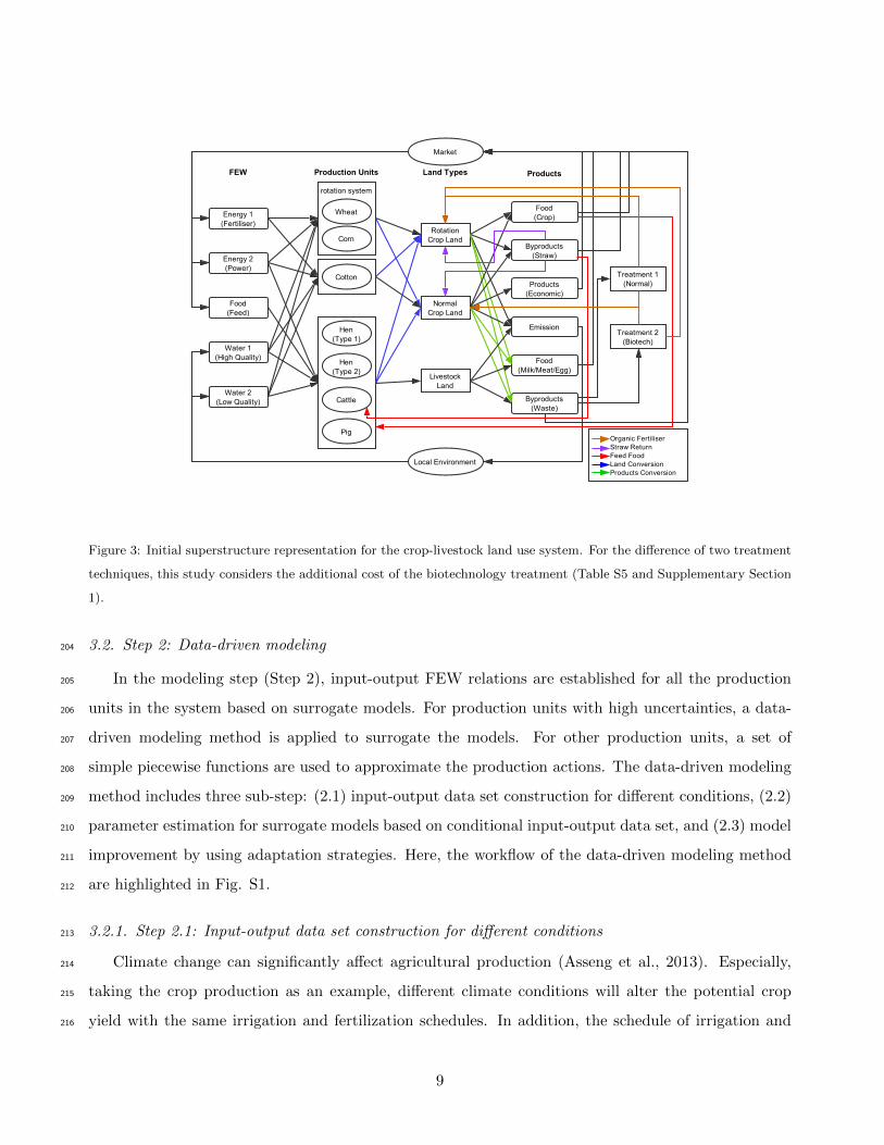
3.1.2. Step 1.2: Superstructure generation193
From the collected data and alternatives involved in the decision-making land use system, a su-194
perstructure is generated. Fig. 3 presents an example of a land use system network considering three195
different food crops and three livestock crops through a superstructure consisting of FEW resources,196
production units, land grids, products and byproducts, known technologies, and FEW-related opera-197
tions that connect them. The superstructure also includes several alternative pathways for resource198
recycling in the system, such as supply resources of feed food, treatment of livestock waste, and routes199
for crop straw use. The size of the decision-making problem depends on the numbers of these elements200
in the superstructure, which can be flexible based on the scales of resources, units, land, and alternative201
technologies and operations. In this study, fertiliser and power use are taken as energy use, there is no202
energy production as we focus on agricultural land use optimization for food production.203
8
Energy 1(Fertiliser)
Energy 2(Power)
Food(Feed)
Water 1(High Quality)
Water 2(Low Quality)
Hen(Type 1)
Hen(Type 2)
Cattle
Pig
Corn
Wheat
Cotton
RotationCrop Land
NormalCrop Land
LivestockLand
Food(Crop)
Food(Milk/Meat/Egg)
Byproducts(Straw)
Products(Economic)
Emission
Byproducts(Waste)
Treatment 1(Normal)
Treatment 2(Biotech)
Local Environment
Market
FEW Production Units Land Types Products
Organic FertiliserStraw ReturnFeed FoodLand ConversionProducts Conversion
rotation system
Figure 3: Initial superstructure representation for the crop-livestock land use system. For the difference of two treatment
techniques, this study considers the additional cost of the biotechnology treatment (Table S5 and Supplementary Section
1).
3.2. Step 2: Data-driven modeling204
In the modeling step (Step 2), input-output FEW relations are established for all the production205
units in the system based on surrogate models. For production units with high uncertainties, a data-206
driven modeling method is applied to surrogate the models. For other production units, a set of207
simple piecewise functions are used to approximate the production actions. The data-driven modeling208
method includes three sub-step: (2.1) input-output data set construction for different conditions, (2.2)209
parameter estimation for surrogate models based on conditional input-output data set, and (2.3) model210
improvement by using adaptation strategies. Here, the workflow of the data-driven modeling method211
are highlighted in Fig. S1.212
3.2.1. Step 2.1: Input-output data set construction for different conditions213
Climate change can significantly affect agricultural production (Asseng et al., 2013). Especially,214
taking the crop production as an example, different climate conditions will alter the potential crop215
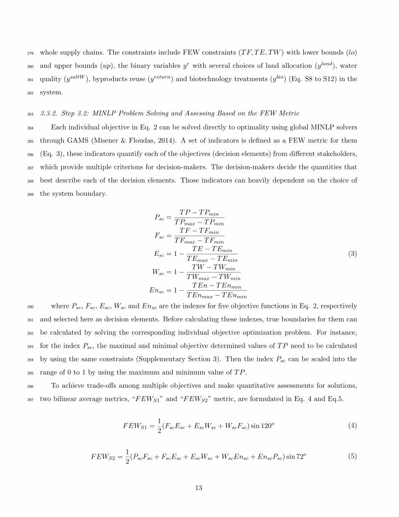
yield with the same irrigation and fertilization schedules. In addition, the schedule of irrigation and216
9
fertilization during productions can also affect the potential yield even with the same water and fertiliser217
input at the same climate conditions. Thus, different climate condition data and schedule data can have218
many combinations, making it extremely difficult for us to obtain data for all the combinations from real219
production processes. To address the data limitation for modeling crop production units, a frequency220
analyse-based method is used to achieve the near-optimal schedules and construct the input-output221
data for modeling under different climate conditions. For each climate condition, a candidate schedule222
set can be constructed based on randomly selected operation times for irrigation and fertilization.223
Simulated experiments of a group of input data points (irrigation and fertiliser, X) are carried out224
through the simulator based on the schedule set. The near-optimal schedules (S) for input water and225
fertiliser can be simply chosen through statistic analysis, that is, counting the frequency of schedules226
with maximum response food yield y for each input data point, the schedules with maximum frequency227
are set as the good choices for crop production in the specific conditions (Details in Supplementary228
Section 2.1).229
3.2.2. Step 2.2: Parameter estimation for surrogate models based on conditional input-output data set230
Note the fact that no single type of surrogate model outperforms all other types for dissimilar231
processes, and choosing the best type of surrogates for each process is a challenging task (Linker &232
Sylaios, 2016). In general, the surrogate model may have better performance by choosing a combination233
of different types of surrogate models rather than using just a single type of surrogate models (Bhosekar234
& Ierapetritou, 2017).235
In this step, a mix-weighted surrogate model is used to estimate the unit production model M .236
The types (k ∈ K) of surrogate functions f(k)θ can be linear, quadratic and reference types, etc. (Frank237
et al., 1990; Wang & Baerenklau, 2014). Thus, in this step the optimization problem of parameter238
estimation for weights ωk and θ(k) of surrogate model Fθ is solved. By using the conditional input-239
output data set {X, y|S}, the proposed method can solve the surrogate modeling problem based on240
the OLS (Ordinary Least Square) approach (Montgomery et al., 2012), cross validation technique and241
a mix-weight method (Goel et al., 2007). Eq. 1 shows the general type of the surrogate models, and242
the detailed methods are in Supplementary Section 2.2.243
Fθ(X) =3∑
k=1
ωkf(k)θ (X) (1)
10
3.2.3. Step 2.3: Model improvement by using adaptation strategies244
Though accurate surrogate models M can be achieved by the above mentioned data-driven mod-245
eling methods based on accurate input-output data, available data for modeling are quite limited in246
reality (Humblot et al., 2017). To address this challenge, as the optimal surrogate model MK based247
on simulating experiments data is generated, an adaptation strategy based on new available data is248
designed to decrease the error ratios of surrogate models (see details in Supplementary Section 2.3 and249
Fig. S3) .250
3.3. Step 3: Multi-objective optimization and assessment251
Since the production units in the system can be described by the proposed modeling methods in252
step 2, a family of unit models are developed to predict their yields. Based on the collected FEW253
data, we can define the land use problem as a multi-objective MINLP problem, and solve it with two254
sub-step: (3.1) Mathematical Formulations for the Multi-Objective Problem, (3.2) MINLP Problem255
Solving and Assessing Based on the FEW Metric.256
3.3.1. Step 3.1: Mathematical Formulations for the Multi-Objective Problem257
The five different objectives for the system are given in Eq. 2: maximal profit (TP ), maximal food258
yield (TF ), minimal energy use (TE), minimal water use (TW ) and minimal environmental penalty259
(TEn). Each individual objective can be solved directly to optimality using the global MINLP solver260
ANTIGONE in GAMS (Misener & Floudas, 2014) (see details in Supplementary Section 3).261
11

maxTP =∑c∈C
∑a∈A
(pcFca − TCca) +∑l∈L
∑b∈B
(plFlb − TClb)
maxTF =∑c∈C
∑a∈A
Fca +∑l∈L
∑b∈B
Flb −∑b∈B
F ′1b
minTE =∑c∈C
∑a∈A
(Eca − E′ca) +∑l∈L
∑b∈B
(Elb − E′lb)
minTW =∑c∈C
∑a∈A
Wca +∑l∈L
∑b∈B
Wlb
minTEn =∑c∈C
∑a∈A
Enca +∑l∈L
∑b∈B
Enlb
s.t.
TF ≥ TF lo
TW lo ≤ TW ≤ TW up
TElo ≤ TE ≤ TEup
yr ∈ {0; 1}; r ∈ R
(2)
where c ∈ C and l ∈ L are production units of crop (C) and livestock (L), respectively. a ∈ A and262
b ∈ B represent cropland grids and livestock land grids. These objectives are calculated based on energy263
(Eca, Elb), water use (Wca,Wlb), economic cost (TCca, TClb), environmental penalty(Enca, Enlb), and264
yield output (Fca, Flb) from different land grids. The total cost for production units (TC) includes their265
related constant cost, energy cost, water cost and other cost (e.g. biotechnology, labor, etc.) (Table266
S5). The energy use for production (E) is the combination of fertiliser, pesticide, irrigation, diesel267
and feed. The water use (W ) mainly comes from irrigation and livestock feeding. The environmental268
penalty (En) in this study only considers the carbon emission and nitrogen leakage . As the framework269
supposes to provide solutions over production years, by choosing recycling pathways, the previous crop270
production in the system can supply part of the food consumed in the livestock production units (F ′1b),271
and the previous wastes (E′ca and E′lb) generated in the crop and livestock production can be converted272
to organic fertiliser used in the crop production, which are regarded as new sources for energy use (the273
fertiliser ratios of waste are shown in Table S3, and the corresponding energy intensities are shown274
in Table S4). Defining appropriate boundaries for any FEW Nexus related systems is a challenge, as275
the FEW Nexus is broad and complex in time and space aspect. Narrow boundaries for the system276
will miss some key impacts, while broad boundaries will increase the model complexity. In this case,277
we define the system boundaries by considering the production on the pieces of land rather than the278
12
whole supply chains. The constraints include FEW constraints (TF, TE, TW ) with lower bounds (lo)279
and upper bounds (up), the binary variables yr with several choices of land allocation (yland), water280
quality (ysaltW ), byproducts reuse (yreturn) and biotechnology treatments (ybio) (Eq. S8 to S12) in the281
system.282
3.3.2. Step 3.2: MINLP Problem Solving and Assessing Based on the FEW Metric283
Each individual objective in Eq. 2 can be solved directly to optimality using global MINLP solvers284
through GAMS (Misener & Floudas, 2014). A set of indicators is defined as a FEW metric for them285
(Eq. 3), these indicators quantify each of the objectives (decision elements) from different stakeholders,286
which provide multiple criterions for decision-makers. The decision-makers decide the quantities that287
best describe each of the decision elements. Those indicators can heavily dependent on the choice of288
the system boundary.289
Psc =TP − TPmin
TPmax − TPmin
Fsc =TF − TFmin
TFmax − TFmin
Esc = 1− TE − TEminTEmax − TEmin
Wsc = 1− TW − TWmin
TWmax − TWmin
Ensc = 1− TEn− TEnminTEnmax − TEnmin
(3)
where Psc, Fsc, Esc, Wsc and Ensc are the indexes for five objective functions in Eq. 2, respectively290
and selected here as decision elements. Before calculating these indexes, true boundaries for them can291
be calculated by solving the corresponding individual objective optimization problem. For instance,292
for the index Psc, the maximal and minimal objective determined values of TP need to be calculated293
by using the same constraints (Supplementary Section 3). Then the index Psc can be scaled into the294
range of 0 to 1 by using the maximum and minimum value of TP .295
To achieve trade-offs among multiple objectives and make quantitative assessments for solutions,296
two bilinear average metrics, “FEWS1” and “FEWS2” metric, are formulated in Eq. 4 and Eq.5.297
FEWS1 =1
2(FscEsc + EscWsc +WscFsc) sin 120o (4)
FEWS2 =1
2(PscFsc + FscEsc + EscWsc +WscEnsc + EnscPsc) sin 72o (5)
13

The metric FEWS1 integrates all the three main indexes of the FEW nexus by using them to298
construct a triangular spider map, presented in Fig. 4a. Therefore, the objective function of the299
optimization problem can be simply converted to the maximization of the graph area combined by the300
three indexes, and the solution can be easily visualized on the spider plot. To create a metric that301
integrates additional decision elements such as profit and environmental cost the FEWS2 metric was302
formulated in Eq. 5 and the spider plot resulting from this index is presented in Fig. 4b. Similarly, the303
multi-objective optimization problem can be converted to the maximum problem of the pentagonal area304
in the spider map. Preliminary results from previous work have verified the effectiveness (Avraamidou305
et al., 2018a,b; Nie et al., 2018; Mroue et al., 2019).306
Fsc
Esc Wsc
●
●●
A
120 °
Psc
Fsc
Esc Wsc
Ensc
●
●
●
●
●
B
72 °
Figure 4: Representation of the composite metric. A: FEWS1; B: FEWS2
4. Results307
We construct a crop-livestock land use system by selecting three crops and three livestock through-308
out three land types among 16-year climate conditions at Yucheng Station (Fig. S2, Table S1). The309
proposed framework solves the land use problem through three sequential steps including design, mod-310
eling, and optimization based on FEW-Nexus in the system, which is a decomposed strategy for solving311
the overall decision-making problem (see Section 3).312
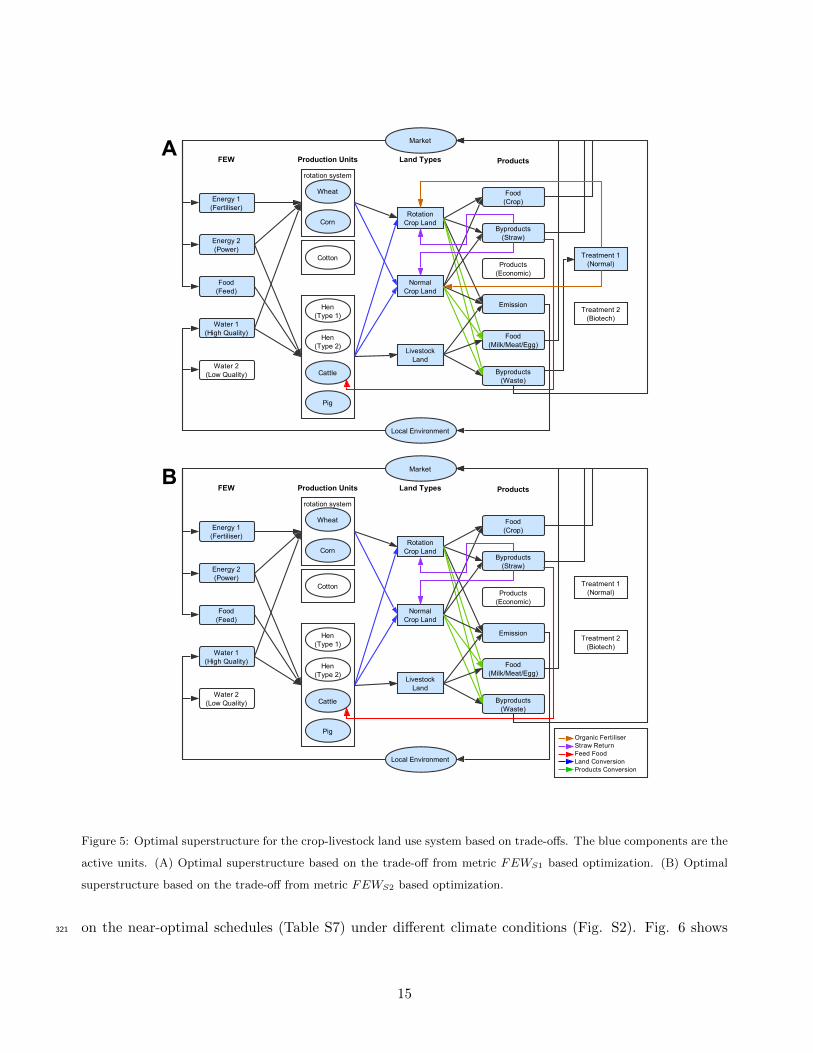
We represent the initial configuration of the crop-livestock land use system with a superstructure313
network in step 1 of the framework (Fig. 3). Fig. 5 shows two optimal superstructures of the system314
based on our trade-off solutions, which are generated by respectively taking the two FEW metrics315
FEWS1 and FEWS2) as integrated objectives to solve the multi-objective optimization problem. The316
optimal superstructures show the general decisions of production units, land allocation, technology317
options, and FEW pathways in the system.318
In step 2, the production units of crop and livestock in the system are modeled. The proposed adap-319
tive data-driven modeling methods (Section 3.2) is used to construct crop yield predictive models based320
14
Energy 1(Fertiliser)
Energy 2(Power)
Food(Feed)
Water 1(High Quality)
Water 2(Low Quality)
Hen(Type 1)
Hen(Type 2)
Cattle
Pig
Corn
Wheat
Cotton
RotationCrop Land
NormalCrop Land
LivestockLand
Food(Crop)
Food(Milk/Meat/Egg)
Byproducts(Straw)
Products(Economic)
Emission
Byproducts(Waste)
Treatment 1(Normal)
Treatment 2(Biotech)
Local Environment
Market
FEW Production Units Land Types Products
rotation system
Energy 1(Fertiliser)
Energy 2(Power)
Food(Feed)
Water 1(High Quality)
Water 2(Low Quality)
Hen(Type 1)
Hen(Type 2)
Cattle
Pig
Corn
Wheat
Cotton
RotationCrop Land
NormalCrop Land
LivestockLand
Food(Crop)
Food(Milk/Meat/Egg)
Byproducts(Straw)
Products(Economic)
Emission
Byproducts(Waste)
Treatment 1(Normal)
Treatment 2(Biotech)
Local Environment
Market
FEW Production Units Land Types Products
Organic FertiliserStraw ReturnFeed FoodLand ConversionProducts Conversion
rotation system
A
B
Figure 5: Optimal superstructure for the crop-livestock land use system based on trade-offs. The blue components are the
active units. (A) Optimal superstructure based on the trade-off from metric FEWS1 based optimization. (B) Optimal
superstructure based on the trade-off from metric FEWS2 based optimization.
on the near-optimal schedules (Table S7) under different climate conditions (Fig. S2). Fig. 6 shows321
15

the cotton predictive model under climate condition 1 as an illustration of good-of-fit performance.322
Fig. 6A shows that the adaptation strategies can efficiently reduce the error ratios when iteratively323
adding new reliable input-output data samples, where strategy 2 has more robust performance. Fig.324
6B shows the final fit performance of the predictive model after limited adaptation times, illustrating325
the mix-weighted predictive model and the models with single types are good enough to simulate pro-326
duction behaviors (error ratio < 2%). By using the adaptation strategies, we can keep on improving327
the fit performance with new data. Fig. S4A shows the relative robust contribution of different single328
model types to the final mix-weighted predictive model when the adaptation iterations increase (i.e.,329
the weights for different types of model vary over narrow ranges). In general, the predictive model of330
crop production units describe the relations between input energy (fertiliser) and water and output331
food yield (Fig. S4B). The optimal parameters, weights, and final error rates for the crop production332
mix-weighted predictive models in three climate conditions are reported by Table S8.333
●
●●
●
●
●
●
●
●
●●
●
● ● ●●
●●
●
●
●●
0.0164
0.0168
0.0172
0.0176
0 1 2 3 4 5 6 7 8 9 10Iteration
Err
or R
atio
(M
ixM
)
Adaption Strategy ● ●s1 s2A
0.000
0.005
0.010
0.015
0.020
Mix type1 type2 type3Model Type
Err
or R
atio
(M
ix)
Error Type Modeling TestB
Figure 6: Good-of-fit performance of adaptive data-driven modeling (e.g. cotton predictive model under climate condition
1). (A) Error ratios of the predictive model based on two adaptation strategies. Strategy 1 (s1) adds new samples without
adjusting bad samples, strategy 2 (s2) adds new samples and removes an equal number of bad samples simultaneously.
(B) Comparisons of final error ratios of the predictive models. The predictive model is a mix-weighted model based on
integration of type1 (linear), type2 (exponential), and type3 (quadratic). The modeling and test error ratios are calculated
by using the cross-validation method.
The livestock production units are modeled with linear and piecewise functions (see Supplementary334
Section 4.1). All the functions show the relations between production time and food yield, as the use335
of input energy and water have been standardized by using known feed formulas (Table S3). Fig. S5336
takes milk production and pig growth as examples to report the fit performance. The results show that337
the fitted data can match the reference data very well (R2 > 0.99).338
16

Interests of different stakeholders are converted into multiple objectives including total profit (TP ),339
total food production (TF ), total energy use (TE), total water use (TW ) and total environmental340
penalty (TEn). In step 3, two FEW metrics (FEWS1 and FEWS2) are designed as the integrated341
objectives of the above multiple objectives and are solved as mixed integer nonlinear programming342
problems (MINLP) efficiently (Section 3.3. Table 2 summarizes the annual trade-off solutions based343
on two FEW metrics and five individual objectives, which include optimal objective values, diverse344
decisions for land allocation, food output, energy and water use, and choices of resources and treatment345
techniques in the system. The optimal solutions allow options for material recycles in the system for346
different objectives.347
Table 2: Optimal solutions for multi-objective optimization (condition 1)
Max TP Max TF Max TE Max TW Max TEn Max FEWS1 Max FESS2
Cropland grid wheat-corn(2) wheat-corn(2) wheat-corn(1) wheat-corn(1) wheat-corn(1) wheat-corn(2) wheat-corn(2)
cotton(1) cotton(1) cotton(1)
Livestock land grid cattle(1) cattle(1) cattle(1) cattle(1) cattle(1) cattle(1) cattle(1)
pig(1) pig(3) pig(1) pig(1) pig(1) pig(1) pig(1)
Profit (Yuan) 1.54E+05 -3.06E+05 -1.26E+06 -1.26E+06 -1.26E+06 5.29E+04 1.01E+04
Food production (MJ) 3.55E+06 4.01E+06 7.15E+05 7.15E+05 7.15E+05 3.01E+06 8.37E+05
Energy use (MJ) 3.97E+06 6.42E+06 4.77E+05 4.77E+05 4.77E+05 1.30E+06 3.92E+05
Water use (t) 1.65E+04 2.69E+05 1.46E+03 40 40 1.53E+04 3.10E+03
Environment Penalty (Yuan) 6.80E+04 9.88E+4 1.40E+03 1.40E+03 1.40E+03 2.61E+04 6.70E+03
Irrigation water high quality high quality high quality - - high quality high quality
Crop byproduct use feed(100%) feed(99.4%) feed(5.6%) feed(5.6%) feed(5.6%) return(0.1%) return(3%)
sell(0.6%) sell(94.4%) sell(94.4%) sell(94.4%) feed(2.2%) feed(3%)
sell(97.7%) sell(94%)
Livestock byproduct use sell(100%) sell(97.2%) sell(100%) sell(100%) sell(100%) sell(62.4%) sell(100%)
return(2.8%) return(37.6%)
Bio-technology treatment no no no no no no no
Feedfood source market market cropland cropland cropland market market
Feedstraw source cropland cropland cropland cropland cropland cropland cropland
TP: total profit; TF: total food production; TE: total energy use; TW: total water use; TEn: total environmental penalty.
Fig. 7 compares the trade-off solutions with individual objective based solutions under climate348
condition 1. Barplots in Fig. 7A compare the relative optimal determined values including production349
cost, food yield, energy use, water use and environmental penalty based on different solutions. Specif-350
ically, the solutions based on minimizing energy use, water use and environmental penalty (TE, TW351
and TEn) have the lowest relative values compared with other objective-based solutions. The solutions352
based on maximizing total profit and food production (TF and TP ) achieve a high level of food output353
but also consume large amounts of resources and make enormous negative impacts on the environment.354
17
As for the trade-off solutions by maximizing the FEW-metrics (FEWS1 and FEWS2), they can achieve355
more food yield (compare with the TE, TW and TEn based solutions) while using fewer resources356
(compare with the TF and TP based solutions). Looking into the compositions of all the considered357
factors, all the solutions suggest that crop productions rather than livestock productions make greater358
contributions to food output, water and energy use, and environmental impacts. Fig. 7B shows the359
solutions of land allocation for different objectives, which illustrate using less land and keeping diversity360
of land use are better strategies than using all the land to produce food. To compare and assess all361
the solutions comprehensively, Fig. 7C shows the results in the spider maps with five indexes, which362
quantitatively represent the five individual objectives respectively. The performance of FEW metric363
based solutions (FEWS1 and FEWS2) is shown in the first and second spider map, illustrating more364
balanced designs for decision making, since they consider several interests of stakeholders at the same365
time (Section 3.3).366
We also analyze the FEW Nexus in the system by taking optimal solutions under climate condition367
1. Fig. S6 and Fig. S7 show that the livestock productions will be stopped at a different time based on368
different objectives, and all the solutions select to allocate livestock land to cattle and pig production.369
Note that minimizing energy, water and environmental penalty will get the same stop times with the370
proposed tradeoff solutions from maximizing the graph area, which is indicated by FEWS1 and FEWS2371
(Fig. S7C). Fig. S8 and Fig. S9 describe the objective-related routes for three main materials in the372
system. The three materials are feed straw for feeding cattle, fertiliser for all the crop production,373
and feed food for feeding all the livestock. These different material supply routes indicate that not all374
the advanced technologies and resource reuse are always necessary for systematic decision-making. For375
instance, the biotechnology for treating livestock waste and organic fertiliser return are not selected376
for the tradeoff decisions (Fig. S8). Even for the solutions that choose organic fertiliser return as one377
kind of fertiliser for crop production, the chemical fertiliser still play the key role and cannot be totally378
replaced (Fig. S8A, Fig. S9B).379
In this study, the lowest food yield at normal climate condition (Condition 1, shown in Fig. S2) are380
used as the lower constraint of food demand in order to compare climate-related performance at the381
same basis. Fig. 8A present the comparisons of relative food yield, energy and water use, environmental382
penalty and production cost for the trade-off solutions at the three climate conditions. The results383
show that generally production at years in condition 1 may achieve more yield and consume fewer384
resources, and consistent decisions can be made for land allocation in different conditions (Fig. 8B).385
The solutions are also evaluated by the FEW metrics (Fig. 8C), which show that the trade-off solutions386
18

255075
200400600
255075
1e+03
1e+07
1e+11
200400600800
FEW−S1 FEW−S2 TP TF TE TW TEn
FEW−S1 FEW−S2 TP TF TE TW TEn
FEW−S1 FEW−S2 TP TF TE TW TEn
FEW−S1 FEW−S2 TP TF TE TW TEn
FEW−S1 FEW−S2 TP TF TE TW TEn
Rel
ativ
e Pr
oduc
tion
Cos
tR
elat
ive
Food
Yie
ldR
elat
ive
Ener
gy U
seR
elat
ive
Wat
er U
seR
elat
ive
Envi
ronm
enta
l P
enal
ty
pig cattle cotton corn wheat
Ass
essm
ent
A
B
C
Land
Use
0 (%)25 (%)50 (%)75 (%)
100 (%)
Fsc
Esc Wsc
Ensc
●
●
● ●
● 0 (%)25 (%)50 (%)75 (%)
100 (%)
Psc
Fsc
Esc Wsc
Ensc●
●
● ●
●0 (%)25 (%)50 (%)75 (%)
100 (%)
Psc
Fsc
Esc Wsc
Ensc●
●
●
●
●0 (%)
25 (%)50 (%)75 (%)100 (%)
Psc
Fsc
Esc Wsc
Ensc
●
●
●●
●0 (%)
25 (%)50 (%)75 (%)
100 (%)
Psc
Fsc
Esc Wsc
Ensc●
●
● ●
●0 (%)
25 (%)50 (%)75 (%)
100 (%)
Psc
Fsc
Esc Wsc
Ensc●
●
● ●
●0 (%)
25 (%)50 (%)75 (%)
100 (%)
Psc
Fsc
Esc Wsc
Ensc●
●
● ●
●
Psc
Figure 7: Comparison and assessment of multiple solutions under climate condition 1. (A) Optimal solutions for multiple
objectives including FEW metrics (FEWS1 and FEWS2), and five individual objectives including total profit (TP), total
food production (TF), total energy use (TE), total water use (TW), and total environmental penalty (TEn). FEWS1
is an integrated index by combining the objectives of total food, energy and water; FEWS2 is an integrated index by
combining all the five individual objectives. The relative optimal determined value and compositions of production cost,
food yield, energy use, water use, and environmental penalty are compared for the seven objectives. (B) Optimal land
allocations for different objective based optimization. Specifically, the green color represent the land grids allocated to
wheat-corn rotation system, and there is no land competition for wheat and corn production. The white color means
the grids are unused. (C) Solution comparison for different objectives. The indexes for five objectives are represented as:
Profit - Psc, Food - Fsc, Energy - Esc, Water - Wsc, Environment - Ensc.
19
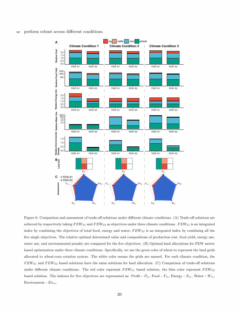
perform robust across different conditions.387
FEW−S1 FEW−S2 FEW−S1 FEW−S2 FEW−S1 FEW−S20.00.51.01.52.0
FEW−S1 FEW−S2 FEW−S1 FEW−S2 FEW−S1 FEW−S2
50010001500
FEW−S1 FEW−S2 FEW−S1 FEW−S2 FEW−S1 FEW−S20.00.51.01.52.0
FEW−S1 FEW−S2 FEW−S1 FEW−S2 FEW−S1 FEW−S2
2.55.07.5
10.012.5
FEW−S1 FEW−S2 FEW−S1 FEW−S2 FEW−S1 FEW−S20.0
0.5
1.0
1.5
Rel
ativ
e C
ost
Rel
ativ
e Fo
od Y
ield
Rel
ativ
e En
ergy
Use
Rel
ativ
e W
ater
Use
Rel
ativ
e En
viro
nmen
tal
Pena
lty
pig cattle corn wheat
0 (%)
25 (%)
50 (%)
75 (%)
100 (%)
Psc
Fsc
Esc Wsc
Ensc
●
●
●●
●
●
●
● ●
●0 (%)
25 (%)
50 (%)
75 (%)
100 (%)
Psc
Fsc
Esc Wsc
Ensc
●
●
● ●
●
●
●
● ●
●
A
B
C
Land
Use
Ass
essm
ent
Climate Condition 1 Climate Condition 2 Climate Condition 3
0 (%)
25 (%)
50 (%)
75 (%)
100 (%)
Psc
Fsc
Esc Wsc
Ensc
●
●
● ●
●
●
●
● ●
●
●
FEW-S1FEW-S2
●
Figure 8: Comparison and assessment of trade-off solutions under different climate conditions. (A) Trade-off solutions are
achieved by respectively taking FEWS1 and FEWS2 as objectives under three climate conditions. FEWS1 is an integrated
index by combining the objectives of total food, energy and water; FEWS2 is an integrated index by combining all the
five single objectives. The relative optimal determined value and compositions of production cost, food yield, energy use,
water use, and environmental penalty are compared for the five objectives. (B) Optimal land allocations for FEW metric
based optimization under three climate conditions. Specifically, we use the green color of wheat to represent the land grids
allocated to wheat-corn rotation system. The white color means the grids are unused. For each climate condition, the
FEWS1 and FEWS2 based solutions have the same solutions for land allocation. (C) Comparison of trade-off solutions
under different climate conditions. The red color represent FEWS1 based solution, the blue color represent FEWS2
based solution. The indexes for five objectives are represented as: Profit - Psc, Food - Fsc, Energy - Esc, Water - Wsc,
Environment - Ensc.
20

5. Discussion388
The case study illustrates that the proposed framework can achieve trade-off solutions to inform389
and assist decision-makers by following three steps: design, modeling, and optimization. Specifically,390
the land use system can be designed as a superstructure network by analyzing the FEW flow and391
nexus; multiple production components in the network can be simulated by using an adaptive data-392
driven modeling method for yield prediction under different climate conditions; and the final trade-off393
solutions for diverse stakeholders can be achieved based on the previous superstructure and models394
by using a FEW metric based optimization method. Our results show that the proposed framework395
provides an effective and consistent methodology for improving, selecting, and assessing systematic396
decisions for land use, which is an innovative try for constructing generic workflows for systematic land397
use considering quantitative FEW-Nexus, effective integration of data and models, and standardized398
metrics for solution selection and assessment.399
Superstructure optimization based approaches have been proven to be cost effective and energy400
efficient for industrial process synthesis and analysis (Yuan et al., 2013). However, its application for401
agricultural process integration is still in the infancy. Food-Energy-Water Nexus (FEW-N), as presented402
in this study, is what makes the superstructure design possible (Hang et al., 2016). From the systematic403
view of FEW-N, we simplify the complicated agricultural system based on input and output FEW flow404
and use the interdependence among diverse process units to combine them, which will generate all the405
possible pathways for the system. Based on the superstructure optimization formulation with desired406
objectives such as maximum food production or minimum water use, we can find optimal process407
topology network without any unnecessary connections and the operating parameters for each units in408
the system simultaneously.409
Recent developments in agricultural modeling and optimization have created increased capabil-410
ity for the management of land use via complicated modeling methods with more parameters (Goel411
et al., 2007). However, the responses of productivity vary widely across different model types and412
region/climate specific data, reflecting differences in the realistic gap between optimal potential yield413
and real yield. The results in the Modeling step of our framework show that the proposed models have414
the robust performance based on limited region and climate specific data compared to previous studies415
(Humblot et al., 2017). This is because the proposed modeling methods use a mix-weighted methods to416
balance the bias performance from different model types, and provides adaptation strategies to keep on417
improving the fit performance of region and climate specific models generated by limited data-driven418
modeling methods. The characters of the our modeling methods illustrate that we can control the neg-419
21
ative impact on data limitations and simplify complicated scientific models for realistic use, which are420
especially important for developing countries who are lacking systematic agricultural databases with421
local details. The adaptation strategies also provide effective ways for improving predictive models and422
accumulating available data.423
Agricultural land is not only farming entity but also known as supplying various products and424
services to multiple stakeholders (Van Ittersum et al., 2008). Such land management is an evolving425
outcome of unremitting negotiation and frequent conflicting interests among the stakeholders. The426
means by which conflicts are settled will be subject to varying supply and demand of FEW, and will427
vary depending on regions and climate conditions (Daher et al., 2019). Thus, the compromise of differ-428
ent stakeholders, and the robust performance with uncertainties are crucially important due to their429
impacts on systematic decision-making for land use. By using the FEW metric based optimization430
method provided by the framework, trade-offs among diverse stakeholders can be achieved most effec-431
tively and consistently. In the optimization step, each of the stakeholder’s objective is formulated and432
normalized by taking their own maximum and minimum optimal values as boundaries. Therefore, all433
the objectives can be transformed into the same scale (e.g., from 0 to 1) by using their own boundaries,434
which provides a consistent basis for comparison and evaluation. All of these scaled objectives can435
be merged together by taking the FEW metric as the integrated objective, which can be visualized436
in spider graphs. We find that the FEW metric based solutions always show more balanced designs437
since it can effectively facilitate the simultaneous farming of diverse goals from stakeholders. Based438
on integrated use of previous FEW data, models, and alternative pathways in the superstructure, the439
assessment results show that the FEW metric based methods also have robust performance when con-440
sidering different climate scenarios, since the framework can adjust the operations in the system to441
keep consistent performance of the land use decisions.442
There is a need for developing methodologies for quantifying policy coherence through quantifying443
the impact of proposed policies across different sectors based on multiple scales, and identify the444
compatibility of current institutional setup and sectional interactions considering the nature of FEW445
resource systems and their interconnections (Daher et al., 2019). The proposed framework designs a446
series of FEW indexes for objectives from different stakeholders, and finally offers a generic metric for447
evaluating and comparing different solution strategies, which provides possibilities for policy-makers448
to adjust policies across different stakeholders, production sectors, and time periods.449
22

6. Limitations and future work450
It is important to discuss some limitations of the developed framework and the potential implications451
of the modeling and optimization methods. First, we assume the schedules calculated base on frequency452
analysis as the “near-optimal” schedules for crop production units. Whilst this choice reduces the453
computational demands of the data-driven modeling, it may result to an underestimation of the real454
potential yield. Future modeling work should seek to model production under dynamic schedules and455
expect to solve the optimization problem of minimizing the gap between simulating yield and real456
potential yield based on optimal schedules.457
A further limitation of the framework is the distribution problem. Our current work focuses on458
the allocated amount of land and FEW resources for different production units with a given area.459
Furthermore, the spatial distribution of different production objects in the land graph has not yet been460
considered. In the future, this can be important for the optimization of supply chains in the land use461
system. We also expect to integrate methods, such as graph theory, to consider the spatial distribution462
of land, FEW, and facilities.463
7. Conclusion464
Meeting the demand for food, energy, and water on a diminishing supply of agricultural land in the465
world without negative environmental impact is a major scientific challenge facing humanity. Despite466
the increasing techniques, data and models, a unified framework to integrate them and make trade-offs467
is lacking. To this end, we propose a framework to facilitate decision-makings based on a Design-468
Modeling-Optimization procedure. Taking an experimental station in China as a model system, our469
framework quantifies the related Food-Energy-Water Nexus, explores trade-offs for diverse stakeholders,470
identifies sustainable pathways for meeting both nature conservation goals and human demand, and471
provides benchmarks for assessing strategies directing alternative pathways. Inspired by the multi-scale472
integration, our methodology should have general utility in complex agricultural systems.473
8. Acknowledgement474
The authors gratefully acknowledge financial supports from STS Project of Chinese Academy of475
Sciences [KFJ-EW-STS-054-3], the Program of China Scholarship Council [201604910976], the National476
Natural Science Foundation of China [61603370], National Science Foundation under Grant Addressing477
23

Decision Support for Water Stressed FEW Nexus Decisions [1739977], and Texas A & M Energy478
Institute.479
References480
Albrecht, T. R., Crootof, A., & Scott, C. A. (2018). The water-energy-food nexus: A systematic review481
of methods for nexus assessment. Environmental Research Letters, 13 , 043002.482
Alexandratos, N., Bruinsma, J. et al. (2012). World agriculture towards 2030/2050: the 2012 revision.483
Technical Report ESA Working paper FAO, Rome.484
Asseng, S., Ewert, F., Rosenzweig, C., Jones, J., Hatfield, J., Ruane, A., Boote, K. J., Thorburn, P. J.,485
Rotter, R. P., Cammarano, D. et al. (2013). Uncertainty in simulating wheat yields under climate486
change. Nature Climate Change, 3 , 827.487
Avraamidou, S., Beykal, B., Pistikopoulos, I. P., & Pistikopoulos, E. N. (2018a). A hierarchical Food-488
Energy-Water Nexus (FEW-N) decision-making approach for land use optimization. In Computer489
Aided Chemical Engineering (pp. 1885–1890). Elsevier volume 44.490
Avraamidou, S., Milhorn, A., Sarwar, O., & Pistikopoulos, E. N. (2018b). Towards a quantitative491
food-energy-water nexus metric to facilitate decision making in process systems: A case study on a492
dairy production plant. In Computer Aided Chemical Engineering (pp. 391–396). Elsevier volume 43.493
Beinat, E., & Nijkamp, P. (1998). Multicriteria analysis for land-use management volume 9. Springer494
Science & Business Media.495
Bergstrom, J. C., Goetz, S. J., & Shortle, J. S. (2013). Land use problems and conflicts: Causes,496
consequences and solutions. Routledge.497
Bertran, M.-O., Frauzem, R., Sanchez-Arcilla, A.-S., Zhang, L., Woodley, J. M., & Gani, R. (2017). A498
generic methodology for processing route synthesis and design based on superstructure optimization.499
Computers & Chemical Engineering , 106 , 892–910.500
Bhosekar, A., & Ierapetritou, M. (2017). Advances in surrogate based modeling, feasibility analysis501
and and optimization: A review. Computers & Chemical Engineering , .502
Chen, Z., Lu, C., & Fan, L. (2012). Farmland changes and the driving forces in Yucheng, North China503
Plain. Journal of Geographical Sciences, 22 , 563–573.504
24

Chiandussi, G., Codegone, M., Ferrero, S., & Varesio, F. E. (2012). Comparison of multi-objective op-505
timization methodologies for engineering applications. Computers & Mathematics with Applications,506
63 , 912–942.507
Daher, B., Lee, S.-H., Kaushik, V., Blake, J., Askariyeh, M. H., Shafiezadeh, H., Zamaripa, S., &508
Mohtar, R. H. (2019). Towards bridging the water gap in texas: A water-energy-food nexus approach.509
Science of the Total Environment , 647 , 449–463.510
Daher, B., Mohtar, R. H., Pistikopoulos, E. N., Portney, K. E., Kaiser, R., & Saad, W. (2018).511
Developing socio-techno-economic-political (STEP) solutions for addressing resource nexus hotspots.512
Sustainability , 10 , 512.513
Dargin, J., Daher, B., & Mohtar, R. H. (2018). Complexity versus simplicity in water energy food514
nexus (wef) assessment tools. Science of The Total Environment , .515
Dhaubanjar, S., Davidsen, C., & Bauer-Gottwein, P. (2017). Multi-objective optimization for analysis516
of changing trade-offs in the Nepalese Water–Energy–Food Nexus with hydropower development.517
Water , 9 , 162.518
D’Odorico, P., Davis, K. F., Rosa, L., Carr, J. A., Chiarelli, D., Dell’Angelo, J., Gephart, J., MacDon-519
ald, G. K., Seekell, D. A., Suweis, S. et al. (2018). The global food-energy-water nexus. Reviews of520
Geophysics, .521
El-Gafy, I. (2017). Water–food–energy nexus index: analysis of water–energy–food nexus of crops522
production system applying the indicators approach. Applied Water Science, 7 , 2857–2868.523
Ellis, E. C., & Ramankutty, N. (2008). Putting people in the map: anthropogenic biomes of the world.524
Frontiers in Ecology and the Environment , 6 , 439–447.525
Fang, Q., Yu, Q., Wang, E., Chen, Y., Zhang, G., Wang, J., & Li, L. (2006). Soil nitrate accumulation,526
leaching and crop nitrogen use as influenced by fertilization and irrigation in an intensive wheat–527
maize double cropping system in the North China Plain. Plant and Soil , 284 , 335–350.528
FAO, U. (2009). How to feed the world in 2050. In Rome: High-Level Expert Forum.529
Flammini, A., Puri, M., Pluschke, L., Dubois, O. et al. (2017). Walking the nexus talk: assessing the530
water-energy-food nexus in the context of the sustainable energy for all initiative. FAO.531
25

Frank, M. D., Beattie, B. R., & Embleton, M. E. (1990). A comparison of alternative crop response532
models. American Journal of Agricultural Economics, 72 , 597–603.533
Garcia, D. J., & You, F. (2016). The water-energy-food nexus and process systems engineering: a new534
focus. Computers & Chemical Engineering , 91 , 49–67.535
Goel, T., Haftka, R. T., Shyy, W., & Queipo, N. V. (2007). Ensemble of surrogates. Structural and536
Multidisciplinary Optimization, 33 , 199–216.537
Hang, M. Y. L. P., Martinez-Hernandez, E., Leach, M., & Yang, A. (2016). Designing integrated local538
production systems: a study on the food-energy-water nexus. Journal of Cleaner Production, 135 ,539
1065–1084.540
Holzworth, D. P., Snow, V., Janssen, S., Athanasiadis, I. N., Donatelli, M., Hoogenboom, G., White,541
J. W., & Thorburn, P. (2015). Agricultural production systems modelling and software: current542
status and future prospects. Environmental Modelling & Software, 72 , 276–286.543
Humblot, P., Jayet, P.-A., & Petsakos, A. (2017). Farm-level bio-economic modeling of water and544
nitrogen use: Calibrating yield response functions with limited data. Agricultural systems, 151 ,545
47–60.546
van Ittersum, M. K., Cassman, K. G., Grassini, P., Wolf, J., Tittonell, P., & Hochman, Z. (2013).547
Yield gap analysis with local to global relevancea review. Field Crops Research, 143 , 4–17.548
Jones, J. W., Antle, J. M., Basso, B., Boote, K. J., Conant, R. T., Foster, I., Godfray, H. C. J.,549
Herrero, M., Howitt, R. E., Janssen, S. et al. (2017a). Brief history of agricultural systems modeling.550
Agricultural systems, 155 , 240–254.551
Jones, J. W., Antle, J. M., Basso, B., Boote, K. J., Conant, R. T., Foster, I., Godfray, H. C. J., Herrero,552
M., Howitt, R. E., Janssen, S. et al. (2017b). Toward a new generation of agricultural system data,553
models, and knowledge products: State of agricultural systems science. Agricultural systems, 155 ,554
269–288.555
Jones, J. W., Hoogenboom, G., Porter, C. H., Boote, K. J., Batchelor, W. D., Hunt, L., Wilkens, P. W.,556
Singh, U., Gijsman, A. J., & Ritchie, J. T. (2003). The DSSAT cropping system model. European557
journal of agronomy , 18 , 235–265.558
26

Keairns, D., Darton, R., & Irabien, A. (2016). The energy-water-food nexus. Annual review of chemical559
and biomolecular engineering , 7 , 239–262.560
Keating, B. A., Carberry, P. S., Hammer, G. L., Probert, M. E., Robertson, M. J., Holzworth, D.,561
Huth, N. I., Hargreaves, J. N., Meinke, H., Hochman, Z. et al. (2003). An overview of apsim, a562
model designed for farming systems simulation. European journal of agronomy , 18 , 267–288.563
Linker, R., & Sylaios, G. (2016). Efficient model-based sub-optimal irrigation scheduling using imperfect564
weather forecasts. Computers and electronics in agriculture, 130 , 118–127.565
McCarl, B. A., Yang, Y., Schwabe, K., Engel, B. A., Mondal, A. H., Ringler, C., & Pistikopoulos,566
E. N. (2017a). Model use in WEF nexus analysis: a review of issues. Current Sustainable/Renewable567
Energy Reports, 4 , 144–152.568
McCarl, B. A., Yang, Y., Srinivasan, R., Pistikopoulos, E. N., & Mohtar, R. H. (2017b). Data for WEF569
nexus analysis: a review of issues. Current Sustainable/Renewable Energy Reports, 4 , 137–143.570
Misener, R., & Floudas, C. A. (2014). Antigone: algorithms for continuous/integer global optimization571
of nonlinear equations. Journal of Global Optimization, 59 , 503–526.572
Mohtar, R. H., & Daher, B. (2018). Lessons learned: Creating an interdisciplinary team and using a573
nexus approach to address a resource hotspot. Science of The Total Environment , .574
Mohtar, R. H., Shafiezadeh, H., Blake, J., & Daher, B. (2019). Economic, social, and environmental575
evaluation of energy development in the eagle ford shale play. Science of The Total Environment ,576
646 , 1601–1614.577
Montgomery, D. C., Peck, E. A., & Vining, G. G. (2012). Introduction to linear regression analysis578
volume 821. John Wiley & Sons.579
Mroue, A. M., Mohtar, R. H., Pistikopoulos, E. N., & Holtzapple, M. T. (2019). Energy portfolio580
assessment tool (EPAT): Sustainable energy planning using the wef nexus approach–texas case.581
Science of The Total Environment , 648 , 1649–1664.582
Nelson, G. C., Valin, H., Sands, R. D., Havlık, P., Ahammad, H., Deryng, D., Elliott, J., Fujimori, S.,583
Hasegawa, T., Heyhoe, E. et al. (2014). Climate change effects on agriculture: Economic responses584
to biophysical shocks. Proceedings of the National Academy of Sciences, 111 , 3274–3279.585
27
Nie, Y., Avraamidou, S., Li, J., Xiao, X., & Pistikopoulos, E. N. (2018). Land use modeling and586
optimization based on food-energy-water nexus: a case study on crop-livestock systems. In Computer587
Aided Chemical Engineering (pp. 1939–1944). Elsevier volume 44.588
Paul, C., Weber, M., & Knoke, T. (2017). Agroforestry versus farm mosaic systems–comparing land-use589
efficiency, economic returns and risks under climate change effects. Science of the Total Environment ,590
587 , 22–35.591
Ramankutty, N., Mehrabi, Z., Waha, K., Jarvis, L., Kremen, C., Herrero, M., & Rieseberg, L. H.592
(2018). Trends in global agricultural land use: implications for environmental health and food593
security. Annual review of plant biology , 69 , 789–815.594
Rathmann, R., Szklo, A., & Schaeffer, R. (2010). Land use competition for production of food and595
liquid biofuels: An analysis of the arguments in the current debate. Renewable Energy , 35 , 14–22.596
Sayer, J., Sunderland, T., Ghazoul, J., Pfund, J.-L., Sheil, D., Meijaard, E., Venter, M., Boedhihartono,597
A. K., Day, M., Garcia, C. et al. (2013). Ten principles for a landscape approach to reconciling598
agriculture, conservation, and other competing land uses. Proceedings of the national academy of599
sciences, 110 , 8349–8356.600
Scanlon, B. R., Ruddell, B. L., Reed, P. M., Hook, R. I., Zheng, C., Tidwell, V. C., & Siebert, S.601
(2017). The food-energy-water nexus: Transforming science for society. Water Resources Research,602
53 , 3550–3556.603
Seppelt, R. (2016). Landscape-scale resource management: Environmental modeling and land use604
optimization for sustaining ecosystem services. Handbook of Ecological Models used in Ecosystem605
and Environmental Management , 3 , 457.606
Sims, R. (2011). Energy-smart food for people and climate. Technical Report UN Food and Agriculture607
Organisation.608
Song, Y., Hou, D., Zhang, J., O’Connor, D., Li, G., Gu, Q., Li, S., & Liu, P. (2018). Environmental and609
socio-economic sustainability appraisal of contaminated land remediation strategies: a case study at610
a mega-site in china. Science of The Total Environment , 610 , 391–401.611
Steduto, P., Hsiao, T. C., Raes, D., & Fereres, E. (2009). Aquacropthe fao crop model to simulate612
yield response to water: I. concepts and underlying principles. Agronomy Journal , 101 , 426–437.613
28

Stewart, T. J., Janssen, R., & van Herwijnen, M. (2004). A genetic algorithm approach to multiobjective614
land use planning. Computers & Operations Research, 31 , 2293–2313.615
Uen, T.-S., Chang, F.-J., Zhou, Y., & Tsai, W.-P. (2018). Exploring synergistic benefits of Water-616
Food-Energy Nexus through multi-objective reservoir optimization schemes. Science of the Total617
Environment , 633 , 341–351.618
Van Ittersum, M. K., Ewert, F., Heckelei, T., Wery, J., Olsson, J. A., Andersen, E., Bezlepkina,619
I., Brouwer, F., Donatelli, M., Flichman, G. et al. (2008). Integrated assessment of agricultural620
systems–a component-based framework for the european union (seamless). Agricultural systems, 96 ,621
150–165.622
Van Tra, T., Thinh, N. X., & Greiving, S. (2018). Combined top-down and bottom-up climate change623
impact assessment for the hydrological system in the vu gia-thu bon river basin. Science of The624
Total Environment , 630 , 718–727.625
Vermeulen, S. J., Challinor, A. J., Thornton, P. K., Campbell, B. M., Eriyagama, N., Vervoort, J. M.,626
Kinyangi, J., Jarvis, A., Laderach, P., Ramirez-Villegas, J. et al. (2013). Addressing uncertainty in627
adaptation planning for agriculture. Proceedings of the National Academy of Sciences, 110 , 8357–628
8362.629
Wang, J., & Baerenklau, K. (2014). Crop response functions integrating water, nitrogen, and salinity.630
Agricultural water management , 139 , 17–30.631
Yuan, Z., Chen, B., & Gani, R. (2013). Applications of process synthesis: Moving from conventional632
chemical processes towards biorefinery processes. Computers & Chemical Engineering , 49 , 217–229.633
Zhang, J., Campana, P. E., Yao, T., Zhang, Y., Lundblad, A., Melton, F., & Yan, J. (2018). The634
water-food-energy nexus optimization approach to combat agricultural drought: a case study in the635
united states. Applied Energy , 227 , 449–464.636
29