A Floristic Study of the Oak Leaf Lake Unit of the Swan

Minnesota State University, Mankato Minnesota State University, Mankato

Cornerstone: A Collection of Scholarly Cornerstone: A Collection of Scholarly

and Creative Works for Minnesota and Creative Works for Minnesota

State University, Mankato State University, Mankato

All Graduate Theses, Dissertations, and Other Capstone Projects

Graduate Theses, Dissertations, and Other Capstone Projects

2016

A Floristic Study of the Oak Leaf Lake Unit of the Swan Lake A Floristic Study of the Oak Leaf Lake Unit of the Swan Lake

Wildlife Management Area in Nicollet County, Minnesota Wildlife Management Area in Nicollet County, Minnesota

Heidi Rauenhorst Minnesota State University Mankato

Follow this and additional works at: https://cornerstone.lib.mnsu.edu/etds

Part of the Botany Commons, and the Plant Biology Commons

Recommended Citation Recommended Citation Rauenhorst, H. (2016). A Floristic Study of the Oak Leaf Lake Unit of the Swan Lake Wildlife Management Area in Nicollet County, Minnesota [Master’s thesis, Minnesota State University, Mankato]. Cornerstone: A Collection of Scholarly and Creative Works for Minnesota State University, Mankato. https://cornerstone.lib.mnsu.edu/etds/608/

This Thesis is brought to you for free and open access by the Graduate Theses, Dissertations, and Other Capstone Projects at Cornerstone: A Collection of Scholarly and Creative Works for Minnesota State University, Mankato. It has been accepted for inclusion in All Graduate Theses, Dissertations, and Other Capstone Projects by an authorized administrator of Cornerstone: A Collection of Scholarly and Creative Works for Minnesota State University, Mankato.

http://cornerstone.lib.mnsu.edu/

http://cornerstone.lib.mnsu.edu/

https://cornerstone.lib.mnsu.edu/



https://cornerstone.lib.mnsu.edu/etds

https://cornerstone.lib.mnsu.edu/etds

https://cornerstone.lib.mnsu.edu/theses_dissertations-capstone

https://cornerstone.lib.mnsu.edu/theses_dissertations-capstone

https://cornerstone.lib.mnsu.edu/etds?utm_source=cornerstone.lib.mnsu.edu%2Fetds%2F608&utm_medium=PDF&utm_campaign=PDFCoverPages

http://network.bepress.com/hgg/discipline/104?utm_source=cornerstone.lib.mnsu.edu%2Fetds%2F608&utm_medium=PDF&utm_campaign=PDFCoverPages

http://network.bepress.com/hgg/discipline/106?utm_source=cornerstone.lib.mnsu.edu%2Fetds%2F608&utm_medium=PDF&utm_campaign=PDFCoverPages

A Floristic Study of the Oak Leaf Lake Unit of the Swan Lake Wildlife Management

Area in Nicollet County, Minnesota

By

Heidi Rauenhorst

A Thesis Submitted in Partial Fulfillment of the

Requirements for the Degree of

Master of Science

In

Biology

Minnesota State University, Mankato

Mankato, Minnesota

April 2016

April 5, 2016



Heidi Rauenhorst

This thesis has been examined and approved by the following members of the student’s

committee.

__________________________________________

Dr. Alison Mahoney, Chairperson

__________________________________________

Dr. Christopher T. Ruhland

__________________________________________

Dr. Forrest Wilkerson

Acknowledgements

I would like to express my gratitude to my committee for their support and

encouragement: Dr. Alison Mahoney, my committee chair, Dr. Christopher T. Ruhland,

and Dr. Forrest Wilkerson. I sincerely appreciate their guidance and insight on this

project. Thank you to Dr. Mezbahur Rahman for sharing his statistical knowledge on this

project and to Desirea Thole for her assistance with the statistical portion of this thesis.

Thank you to Joe Stangel with the Minnesota Department of Natural Resources

Nicollet Area Wildlife Office for his assistance in my research of this project. His

knowledge and resources of the Oak Leaf Lake Unit were incredibly helpful.

I would like to thank my mom, Deb, for her support and for all the times she

helped me out. Words cannot express my gratitude. Thank you to my son, Isaac, for

being an all-around great kid and my motivation to complete this project.



Heidi Rauenhorst

Master of Science in Biology

Minnesota State University, Mankato, MN

April 2016

Prairies play an integral ecological role, protecting biodiversity and providing habitat for

fauna. The number of prairie acres has significantly declined in Minnesota, making the

existing prairies that much more valuable. The Oak Leaf Lake Unit of the Swan Lake

Wildlife Management Area in Nicollet County, Minnesota (latitude 44.311050, longitude

-94.015577) was purchased by the Minnesota Department of Natural Resources in 1994

and is being managed as tallgrass prairie. Floristic surveys were performed during the

2011 and 2012 growing seasons to gather baseline data. These data were used to assess

the quality of the site through calculation of various indices that allowed comparison of

its flora to floras of other prairies in the area. Two sampling methods, a walk-through

method and a random-sampling-in-quadrats method, were employed to compare the

effectiveness of data compilation (i.e. the number of plant species located and identified)

for each method. Additional data collected via the random-sampling-in-quadrats method

included percent cover, litter depth, frequency, and species diversity. In total, 112 plant

species in 88 genera and 33 families were found over both growing seasons with nearly

half found exclusively using the walk-through method in 2011 and none found

exclusively using the random-sampling-in-quadrats method in 2012. The percentage of

native, nonnative, and unknown species located in each sampling method were similar.

No rare or endangered species were located. Differences in the sampling methods make

determining the most effective and efficient method difficult. The most effective method

is determined predominantly by the goals and restrictions of each distinct study. For

the purposes of this particular study, the walk-through method produced a more

complete compilation of plant species data than the random-sampling-in-quadrats

method. The data gathered through this study provides important information on the

current ecological quality of the Oak Leaf Lake Unit while providing a baseline for future

research at the site.

i

TABLE OF CONTENTS

Acknowledgements

Abstract

Table of Contents i

List of Tables and Figures iv

Introduction 1

Prairies in Minnesota 1

Prairie Characteristics 5

Site Description 7

Geology 9

Soils 9

Hydrology 11

Previous Site Surveys 12

Terminology and Designators for Plant Classes 13

Floras and Floristic Surveys 18

Vegetation and Vegetation Surveys 20

Physiological Requirements of Plants 21

Succession 23

Data Collection Methods: Walk-Through and Random-Sampling-in-Quadrats 25

The Walk-Through Method 25

The Random-Sampling-in-Quadrats Method 25

Data Collection and Analysis 28

ii

Data Collected and Indices Calculated 28

Statistical Analyses 33

Taxonomy 33

Objectives 34

Hypotheses 35

Methods 35

Precipitation and Temperature Data for 2011 and 2012 35

Floristic Survey 2011 37

Random Sampling 2012 38

Results 41

Precipitation and Temperature Data for 2011 and 2012 41

2011 Walk-Through Method 46

2012 Random-Sampling Method 49

Distribution of Species within Three Site Sections (A, B, C) 52

Discussion 54

Flora at the Oak Leaf Lake Unit 54

Early-Successional Species and Weeds 58

Assessing the Site’s Diversity and Quality 60

Species Richness 64

Species Diversity 66

Comparison of Three Sections Within the Site 68

Effects of Weather and Climate on the Flora at the Oak Leaf Lake Unit 72

iii

Comparison of Data Collection Methods 74

Choosing the Best Sampling Method and Time to Collect Data 74

Conclusion 77

Recommendations 81

Literature Cited 84

Appendix A. Maps of Oak Leaf Lake Unit 92

Appendix B. Soils and Sections Map of Oak Leaf Lake Unit 95

Appendix C. Soil Types Found at the Oak Leaf Lake Unit as Determined by USDA 96

Appendix D. Plant Species and Collection Data from the 2011-2012 Oak Leaf

Lake Unit Survey 98

Appendix E. Life History Data, Ecological Requirements and Indicator/Weed

Status for Plant Species at the Oak Leaf Lake Unit 105

Appendix F. Species Area Curves for the Early-, Mid-, and Late-Blooming/Fruiting

Periods of the Random Sampling Method 112

Appendix G. Early-Successional, Nonnative, Invasive, Noxious, and High-Quality

Indicator Species Found at the Oak Leaf Lake Unit, the Section(s)

Within Which They Were Located and Their Wetland Codes 114

Appendix H. Indices for Analyses of Data Collected in This Study, Along With

Their Calculations and Purpose 116

Appendix I. Photographs of Oak Leaf Lake Unit 117

iv

List of Tables and Figures

Figure 1. Three biomes in Minnesota (used with permission from MN DNR) 2

Table 1. Range description and values for the Palmer Hydrological Drought Index 36

Table 2. Cover class and corresponding percent cover. 40

Table 3. Mean monthly precipitation for the growing season for 1981 – 2010 mean

and monthly precipitation in 2011 and 2012. 42

Figure 2. Mean daily precipitation per growing season month for 1981 – 2010,

2011, and 2012. 42

Table 4. Mean monthly temperature for the growing season for 1981 – 2010 mean

and monthly precipitation in 2011 and 2012. 43

Figure 3. Mean daily temperatures per growing season month for 1981 – 2010,

2011, and 2012. 44

Figure 4. Monthly Palmer Hydrological Drought Index values for the growing

seasons of 2011 and 2012 45

Figure 5. Mean number of days in the growing season for 1981-2010 and number

of days in the in the growing season for 2011 and 2012 46

Table 5. Top five most frequently-located species for each sampling event and

for the full season for the random sampling method. 51

Table 6. Mean cover class for each sampling event and for the full season for

each cover category. 51

Table 7. Species located in Sections A, B, and C for 2011 and 2012. 53

Table 8. Summary of the floristic data collected at the Oak Leaf Lake Unit. 60-61

Table 9. Jaccard’s coefficients comparing the flora at the Oak Leaf Lake Unit with

floras of 11 predominantly-grassland sites within Minnesota. 63

Table 10. C-values and wetland rating classes per the Army Corps’ wetland

classification system and Ladd's numerical classification of species at

Oak Leaf Lake Unit and Kasota Prairie SNA 66

v

Table 11. Wetland codes for all species located in each section of the Oak Leaf

Lake Unit 70

Table 12. Wetland codes for indicator species located in each section of the Oak

Leaf Lake Unit 70

Figure A1. Location of the Oak Leaf Lake Unit in Nicollet County, Minnesota. 93

Figure A2. Map of the Oak Leaf Lake Unit and surrounding land. 94

Figure B1. Soils and sections map of Oak Leaf Lake Unit. 95

Table C1. Soil types found at the Oak Leaf Lake Unit as determined by USDA. 97

Table D1. Plant survey data from the 2011-201 2 2011 Oak Leaf Lake Unit. 99

Table E1. Life history data, ecological requirements and indicator/weed status

for plant species at the Oak Leaf Lake Unit. 106

Figure F1. Species area curve for the early-blooming/fruiting period of the random

sampling method. 112

Figure F2. Species area curve for the mid-blooming/fruiting period of the random


Figure F3. Species area curve for the late-blooming/fruiting period of the random


Table G1. Early-successional, nonnative, invasive, noxious, and high-quality

indicator species found at the Oak Leaf Lake Unit, the section(s) within

which they were located and their wetland codes. 114

Table H1. Indices for analyses of data collected in this study, along with their

calculations and purpose. 116

Figure I1. Photograph of the signage at the Oak Leaf Lake Unit taken on June 19,

2011. 117

Figure I2. Photograph of the Oak Leaf Lake Unit taken on June 26, 2011. 118

Figure I3. Photograph of the Oak Leaf Lake Unit taken on August 6, 2011. 119


vi


Figure I6. Photograph of the Oak Leaf Lake Unit taken on September 23, 2011. 122

1

INTRODUCTION

Prairies play an integral ecological role. They are essential in protecting

biodiversity and are a necessary habitat for fauna. Prairie floras exist under diverse

growing conditions and niches.

A floristic study and analysis of the Oak Leaf Lake Unit of the Swan Lake

Wildlife Management Area was performed to gather baseline data and to compare two

sampling techniques. Baseline data are needed because little floristic information exists

for this site and will be beneficial for management and future research. Two different

plant sampling techniques were employed to compare and contrast the effectiveness of

the techniques. The first technique employed a walk-through method, where the study

site was thoroughly walked through on 13 occasions and specimens of all plant species

found were collected as vouchers. The second technique employed a random-sampling-

in-quadrats method that only recorded species found within 1 m2 quadrats located

randomly throughout the site. The efficacy of one sampling technique over the other is

often debated. Species richness and distinctiveness of the plant species collected were

analyzed for each method to rank the effectiveness of each method. Findings indicated

each sampling method had strengths and weaknesses. The plant species and vegetation

found at Oak Leaf Lake are essential in determining the ecological quality of the site.

Prairies in Minnesota

Earth is divided into major ecological regions called biomes, which are classified

by their vegetation, which is controlled by climate, topography, proximity to large bodies

2

of water, soil, and other factors (Carpenter 1940; Dice 1962; Tester 1995). Three biomes

occur in Minnesota: coniferous forest, deciduous forest, and prairie. (Figure 1) (MN DNR

1993; Tester 1995).

Figure 1. The three biomes in Minnesota: coniferous forest, deciduous forest, and prairie. The study area is located at the transitional area, or ecotone, of the deciduous forest and prairie biomes (from MN DNR, Minnesota’s native vegetation: a key to natural communities, version 1.5. Copyright © 1993 by State of Minnesota, MN DNR. Reprinted by permission of MN DNR).

Oak Leaf Lake Unit

3

Physical environmental factors, such as temperature and precipitation, drive the

development and succession of biomes and communities (Dice 1962). Low precipitation

and warm summers and cold winters were instrumental in the development of the prairies

of southwestern and southcentral Minnesota (Carpenter 1940; Tester 1995), where the

Oak Leaf Lake Unit is located. Frost also shapes communities as it can affect the

growing season by injuring, delaying growth, or killing individuals (Dice 1962).

Coniferous forest is found in northeast Minnesota where average annual

temperatures range between 2.2 and 5° C and average annual rainfall is 45.7 to 50.8 cm

(MN DNR 2016a). It is dominated by Pinus strobus (white pine), P. resinosa (red pine),

Picea spp. (spruce), Abies spp. (fir), Populus spp. (aspen), and Betula spp. (birch) (Tester

1995). Deciduous forest occurs in a narrow diagonal band running from the northwest to

the southeast where average annual temperatures range between 3.9 and 7.2° C and

average annual rainfall is 40.6 to 45.7 cm (MN DNR 2016a). It consists mainly of

hardwoods including Acer spp. (maple), Tilia spp. (basswood), and Quercus spp. (oak) in

upland areas; low, wetter areas support Ulmus spp. (elm) and Acer spp. (maple) (Curtis

1971; Tester 1995). Prairie occurs in the west from Canada to Iowa where average

annual temperatures range between 2.8 and 7.2° C and average annual rainfall is 35.6 to

40.6 cm (MN DNR 2016a); it extends further east in the central and southern portion of

the State where annual precipitation would support deciduous forest. In this region

prairies were usually maintained by periodic fires. Prairie is mostly made up of

herbaceous plants, often divided into two informal groups: grasses (grass and grass-like

species) and forbs (non-grass-like species) (Tester 1995). The study site is located on the

4

eastern edge of the prairie biome near the ecotone (the transitional area between two

biomes or communities [Carpenter 1940; Dice 1962]) of the prairie biome and the

deciduous forest biome. The ecotone between the prairie and deciduous forest is often

brush prairie, consisting of areas of small trees, low shrubs, and herbaceous species, or

savanna, consisting of scattered trees with herbaceous species underneath (Tester 1995).

Minnesota was once home to more than 7.28 million ha of native prairie

(Marschner 1974), but now, less than two percent, roughly 95,100 ha, remains (MN DNR

2010; MPPWG 2011). Seven primary threats to the remaining native prairie and

associated habitat have been identified by the Minnesota Prairie Plan Working Group

(MPPWG 2011): 1) continued loss of prairie and wetlands to conversion, development,

and destruction, 2) invasive species, 3) detrimental grazing practices, 4) woody plant

encroachment, 5) energy development, 6) atmospheric nitrogen deposition, and 7) change

in climate. Many prairies are too fragmented and too small to provide adequate habitat

for many species (Higgins el al. 2001; MPPWG 2011), thus threatening sustained

biodiversity (Gibbs et al. 2008).

Human activity is primarily responsible for the destruction of most of

Minnesota’s native prairie. Land was cleared predominantly for agricultural use and

urban development (Samson et al. 2004). Approximately 1.27 million ha of restored

prairie exists in Minnesota; of that, 647,500 ha are enrolled in the United States

Department of Agriculture’s (USDA) Conservation Reserve Program (CRP) (BWSR

2010). Nearly 44 percent of those 647,500 CRP ha (over 284,500 ha) expired or will

expire in Minnesota between September 2014 and September 2018 (USDA 2014). Once

5

expired, landowners, for the most part, are free to do what they wish with their CRP

property, including destroying the prairie established with their CRP contract.

Prior to European settlement, prairies of south-central Minnesota were maintained

by disturbances of fire, changes in weather (i.e. drought), and grazing by large

herbivores, mainly bison (Samson et al. 2004; MPPWG 2011). Fires were either

naturally-occurring, usually ignited by lightning, or intentionally set by humans who

routinely used fire to clear out old, dead plant debris to promote new plant growth

(Samson et al. 2004). Prairie fires usually moved eastward, driven by southwestern

winds, until they reached the forest and died out, due to greater moisture and less easily

ignitable fuel (Tester 1995). The deciduous forest was limited in its spread westward by

prairie fire; thus, fire played a role in the development of the ecotone between the prairie

and deciduous forest (Tester 1995).

Prairie Characteristics

Prairies are diverse communities dominated by herbaceous perennials, species

that store starch in extensive roots and/or underground stems (rhizomes), and/or in

modified underground stems (bulbs, corms, tubers, etc.) (Raven et al. 2005; Solomon et

al. 2005). In temperate regions, aerial stems die to the ground each fall. The plants

overwinter underground on stored reserves in their “perennating organs” (roots,

rhizomes, bulbs, corms, tubers, etc.). In spring, buds on perennating organs begin to

develop to produce new sets of aerial stems, leaves, and, eventually, reproductive

structures. In contrast to shrubs and trees, which produce wood that requires high-energy

6

input but is not photosynthetic, the entire aerial shoot system of herbaceous perennials is

mostly photosynthetic, making prairies among the most productive biomes on the planet

(Kline 2005; Raven et al. 2005; Solomon et al. 2005).

Prairie species are adapted to extremes of temperature (daily and seasonal), high

light intensity, desiccating winds, grazing, fire, drought, and often, nutrient-poor soils

(Tester 1995; Kline 2005; Gendron and Wilson 2007). Most share abilities to 1) grow

quickly under a wide range of conditions, such as varying levels of moisture and nitrogen

availability, 2) reproduce asexually (vegetatively/clonally) by rhizomes or roots that are

protected from aboveground disturbances such as fire and grazing, 3) reproduce sexually

through the production of numerous seeds to increase probability of regeneration (Grilz

and Romo 1994; Gendron and Wilson 2007; USDA 2012c; Tompkins et al. 2013).

Grasses, in particular, take advantage of wind for both pollination and seed dissemination

(Kline 2005).

The Asteraceae (sunflower), Poaceae (grass), and Fabaceae (legume),

respectively, are the best-represented families in prairies (Dix and Butler 1960; Kline

2005). Prairies are dominated by grasses, both in biomass and cover, however they do

not contribute the most to prairie plant diversity. Ladd (2005) provides a list of 988

tallgrass prairie species. Annual and perennial sedges and grasses make up about 20

percent of the species. Among the most common native true grasses in drier Midwestern

prairies are Schizachyrium scoparium (little bluestem), Bouteloua curtipendula (side-oats

grama), Sporobolis heterolepis (prairie dropseed), and Stipa spartea (porcupine grass)

(Tester 1995; Kline 2005). In deep silt-loam soils of dry to mesic sites Andropogon

7

gerardii (big bluestem) and Sorghastrum nutans (Indian grass) are very common; in

wetter sites one finds Calamagrostis canadensis (blue joint grass) and Spartina pectinata

(prairie cord grass) (Tester 1995; Kline 2005). Commonly abundant nonnative perennial

grasses include Bromus inermis (smooth brome) (Grilz and Romo 1994) and Poa

pratensis (Kentucky bluegrass), which forms a dense sod once established; it is often

included in seed mixes used to stabilize roadsides (USDA 2012c). Forbs provide the

diversity on prairies, making up as much as 70 percent of species on a site (Ladd 2005);

they are usually abundant, with their composition varying with soil depth, moisture, and

the age of the site (Kline 2005). Charismatic prairie species are found in

Symphyotrichum (aster [formerly genus Aster]), Solidago (goldenrod), Ratibida and

Rudbeckia (coneflowers), Helianthus (sunflower), Asclepias (milkweed), Monarda

(mints), to name only a few genera (Curtis 1971; Tester 1995; Kline 2005; USDA

2012c).

In mature prairies, species are usually long-lived, slow-growing, late-successional

perennials that grow close together, reducing the likelihood that invasive species can

become established (Kline 2005). In young or disturbed, low-quality prairies, short-

lived, fast-growing, early-successional annuals can often be found.

Site Description

The Oak Leaf Lake Unit is located in the northern half of section 25 of Oshawa

Township (T110N R27W) in Nicollet County about 2 km west of Saint Peter, Minnesota

(latitude 44.311050, longitude -94.015577) (Figure A1) in an area where, historically,

8

prairies (maintained by fire) and maple-basswood climax vegetation formed patches on

the landscape. The 25.9 ha unit comprises a 4.78 ha lake that is a resting and feeding

location for migratory birds, 0.24 ha of deciduous forest, 3.08 ha of seasonally-flooded

emergent vegetation, and 17.80 ha of restored tallgrass prairie, which was seeded with

prairie grasses and forbs (MN DNR 2012b). The land surrounding the unit includes a

farm site to the east and rotational cropland planted predominantly to corn and soybeans

(Figure A2).

The unit was purchased by the MN DNR in September 1994 to become “part of

the Swan Lake Wildlife Management Area and to be managed for waterfowl nesting

cover, upland game bird nesting cover, nongame use, prairie propagation and public

recreation” (MN DNR 2011). Some of the wildlife documented at the unit include

mallards, teals, wood ducks, great blue herons, egrets, shore birds, gulls, pheasants,

muskrats, and white-tailed deer (MN DNR 2011). Artificial nest structures were in place

in the past, including mallard baskets, wood duck boxes, round bales for geese, and

bluebird houses (MN DNR 2011), and some are still in place. Hunting is allowed at the

unit.

There are 1.05 ha of wetlands located on the east side of the site classified as

Type 4 wetlands, which are inland deep fresh marshes that usually have soils covered

with 15 cm to 0.9 m of water during the spring and summer and support species like

cattails, reeds, bulrushes, spike-rushes, and wild rice (BWSR n.d.). Type 4 wetlands

often fill shallow lake basins or potholes or border open water. In the case of this study

site, the wetlands border the open water of Oak Leaf Lake.

9

The study site consists of a portion of the Oak Leaf Lake Unit of approximately

6.95 ha on the northern end of the unit, along the northern shoreline of the lake

(Figure B1).

Geology

Three different rock layers of three different ages underlie the study site (Jackson

1994; Ellingson 2000). Granite, gneiss, and quartzite are the primary components of the

oldest layer from the Precambrian Period, approximately 1.5 to 3 billion years ago. The

second layer, deposited about 570 to 480 million years ago during the Paleozoic Period,

consists of sandstone and dolomite. The third layer, the surficial layer made up of loamy

till, was left behind by the region’s most recent Wisconsin Period glaciers about 12,000

years ago (Jackson 1994; Ellingson 2000). As the glaciers advanced, retreated, or

melted, glacial sediments, a mixture of clay, silt, sand, gravel, cobbles, and boulders,

were deposited, creating a topography of gently sloping to nearly level “ground

moraines” (Jackson 1994; Ellingson 2000). Erosion of these moraines created the

landscape we know today. Glacial sediments found at the study site are classified as

Gently Rolling Ground Moraine Sediments (Jackson 1994; Ellingson 2000).

Soils

Soil is a mixture of inorganic and organic particles in which plants grow. Soils

can differ greatly in organic matter, texture, pH, and depth and therefore play an

important, but varied, role in the development of biomes and communities (Dice 1962).

10

Soil texture is defined by the percentages of sand (particles with diameters between 2 and

0.5 mm), silt (with diameters between 0.5 and 0.002 mm), and clay (with diameters less

than 0.002 mm) (Dice 1962). Larger-sized particles, such as gravel (with diameters

greater than 2 mm), pebbles, and cobbles may also be present. Soils with larger particle

diameters often have more open spaces and can better allow plant roots and rainfall to

penetrate (Dice 1962). Particle size also affects evaporation rates, water retention, and

rates of oxygen and carbon dioxide diffusion; these factors, along with climate, affect the

type of biome or community that develops (Dice 1962).

Most prairie soils are covered with a layer of plant litter, which is the dead plant

material that has fallen to the ground and is an essential part of the nutrient cycle and soil

health (Collins and Wallace 1990). Litter can foster plant growth by providing

appropriate moisture, temperature, and soil nitrate levels for increased seed germination

(Myster 2006). But litter can also deter plant growth by physically blocking seedlings,

obstructing sunlight, or providing conditions that promote fungal growth (Carson and

Peterson 1990; Higgins et al. 2001; Myster 2006). Litter depth is a measurement of the

accumulated plant litter that, once decomposed, becomes organic matter in the soil and

provides nutrients for plant uptake (Myster 2006).

According to the USDA, no highly erodible land exists on the site (USDA n.d.).

The highest elevation of the grassland area is approximately 305 m and slopes down to its

lowest level, 301 m, at the lake. An analysis of USDA soil maps shows four types of

soils found at the site (Table C1). The western half from the driveway and parking lot to

the middle consists of 109–Cordova clay loam (fine loamy) (Figure B1). The middle

11

portion on the eastern side consists of 239–Le Sueur clay loam (fine loamy). The

northwest portion and the middle of the eastern half consists of 978–Cordova-Rolfe

complex (fine loamy). The shoreline consists of 1075–Klossner and Muskego soils,

ponded (loamy). The organic matter content is highest in the 1075–Klossner and

Muskego soils, with 25 to 60 percent, while the other three soil types have an organic

matter percentage ranging from two to seven. The decomposition of the prairie plant

roots and the litter produced every year by the prairie vegetation contribute organic

matter and nutrients to the soil (Tester 1995). All four soil types found at the study site

have slopes ranging from zero to three percent, are classified as very-poorly-drained to

somewhat-poorly-drained, and have a high- to very-high available water capacity. The

amount of water the soil can store that is available for plant use is based partly on soil

particle size and soil compaction (Dice 1962). The roots of plants are not able to extract

all of the water in the soil and each plant species is able to extract water at different rates

depending on their water needs, root system, and transpiration rate (Dice 1962). The

least porous layers of all four soil types have moderately low to moderately high

capacities to transmit water (capacity is determined by how much water in inches can be

transmitted per hour).

Hydrology

Aquifers consist of a permeable layer or layers of rock and/or sand that can hold

water. Many aquifers are found in eastern Nicollet County where the Oak Leaf Lake

Unit is located. The aquifers are located within the sandstone from the Precambrian and

12

Paleozoic eras and contain water with high concentrations of iron, sulfate, and dissolved

minerals leached from the sandstone (Jackson 1994).

Two small marsh wetlands, one on the northeast side of the lake and the other

located west of the lake, drain into the lake. The northeast wetland is located within the

study site and the west wetland is outside of the study site boundaries. Several small

springs flow into the lake on the northeast side, but the major source of water for the lake

is local runoff (MN DNR 2011). The surrounding land has a cropping history of corn

and wild rice and contains drainage tile near the lake but due to poor records, the exact

location of the tile is unknown. Records do indicate, however, approximately 2,100 m of

tile were present in 1982 in parcels adjacent to the site (MN DNR 2011). The lake

contains no outlet, limiting the potential for extreme changes in water levels and possibly

retarding the growth of emergent vegetation (MN DNR 2011). The lake is currently

classified as a “protected public water” under the Protected Waters Inventory

Classification (MN DNR 2011).

Previous Site Surveys

A 1953 survey of the site was carried out on July 14 and 15; it focused on Oak

Leaf Lake (MN DNR 2011), which was described as a semi-permanent waterfowl and

muskrat lake approximately 85.7 ha in size with 2.3 km of shoreline. The survey (MN

DNR 2011) noted the following: the maximum depth of the lake was 1.7 m and mean

depth was 1.2 to 1.4 m. The lake bottom was predominantly firm mud. Of the 24 aquatic

plant species identified, 10 were emergent (the plant is rooted in water, but the majority

13

of the plant extends out of the water), with eight native and two of unknown origin, and

14 were submergent (the majority of the plant, if not all, grows under the water’s

surface), with 12 native and two of unknown origin. The shoreline slope was gradual

with species in Populus (cottonwood and poplar), Ulmus (elm), Salix (willow), and

Quercus (oak). Approximately 70 percent of the shoreline was used for pasture but only

the northwest portion was heavily grazed.

Another survey was conducted 38 years later in 1991. The survey (MN DNR

2011) noted the following: the shoreline length was 4.8 km, 2.5 km more than in 1953,

the maximum depth of the lake was 0.9 m, 0.8 m less than in 1953, and the median depth

was 0.9 m, 0.3 to 0.5 m less than in 1953. The lake bottom was described as muck. Nine

aquatic plant species were located in 1991 while 24 were located in 1953. All nine

species located in 1991 were submergent, with eight native and one of unknown origin.

Four of the submergent native species were located in both 1991 and 1953.

Terminology and Designators for Plant Classes

Plant-related terminology is extensive and very often used imprecisely. This report

uses definitions for native, nonnative, exotic, translocated, naturalized, adventive,

ornamental, weed, early-successional, noxious species, invasive species, forbs, grass, and

indicator species as defined in “Native, Invasive, and Other Plant-Related Definitions”

(USDA 2012b) and other sources as follows:

A native plant species has evolved in a particular region over a period of

hundreds or thousands of years, without human intervention (Fernald 1950; USDA

14

2012b). In this study, natives are those species that were present in North America

before European settlement.

Nonnative or introduced plant species occur in areas where they have not

previously been located. Most nonnatives were introduced by humans intentionally or

accidentally (USDA 2012b). An exotic plant is one that is nonnative to the continent

where it is currently found growing (USDA 2012b). For example, a plant species native

to China would be considered exotic in the United States. Translocated plant species

differ from exotic plant species in that they are found in a different region of their native

continent. For example, a plant species native to Florida would be considered

translocated in California.

Nonnatives that persist in new locations and begin to reproduce without human

assistance are said to be naturalized. Naturalized plant species are often found near

areas of human disturbance (USDA 2012b) because they are often early-successional

species, introduced accidently, or have escaped from horticultural or agricultural settings

into natural areas (Curtis 1971). Some nonnative species become widely and

permanently established while others only persist within specific habitats or exist

temporarily because conditions are temporarily ideal for their maintenance and

propagation. Such species are referred to as adventive (Muehlenbach 1969). Nonnative

plants that cannot reproduce without human assistance and are generally found in

horticultural and agricultural settings are called ornamentals (USDA 2012b).

Ralph Waldo Emerson (1878) famously defined a weed as “a plant whose virtues

have not yet been discovered.” Generally speaking, a weed is a plant growing in a place

15

where it is not wanted, so therefore what constitutes a weed is highly subjective; a plant

that is desirable to one person may be undesirable to another. Traditionally, weeds are

defined as objectionable and undesirable plants that disrupt human activities or health

(Hamill et al. 2004) or interfere with management goals and plans (Randall 1996). Many

species classified as weeds by the University of Minnesota Extension (UM-Ext) (2015a,

2015b, 2015c), Minnesota Department of Agriculture (MDA) (2010, 2012), and Gleason

and Cronquist (1991) are actually early-successional species such as native annual

species Conyza canadensis (horseweed), and species in Chenopodium (lamb’s quarters)

and Amaranthus (pigweed). These “pioneer species” grow in open disturbed sites

because of their ability to endure environmental extremes and utilize limited resources

(Bazzaz 1974). As early-successional species increase in density, they change

environmental conditions by decreasing soil temperature and increasing nutrient

availability, which creates suitable growing conditions for mid- and late-successional

species. Eventually, mid- and late-successional plant species, herbaceous perennials and

shrubs in a prairie, crowd out early-successional annual species like horseweed, lamb’s

quarters, and pigweeds (Curtis 1971; Foster and Tilman 2000). Naturalized nonnative

annuals, biennials, and short-lived perennials such as Thlaspi arvense (field pennycress),

Bromus commutatus (hairy chess brome), and Taraxacum officinale (dandelion) serve the

same function. In the context of this study, annual and other short-lived pioneer species

listed as weeds by the UM-Ext (2015a, 2015b, 2015c), MDA (2010, 2012), and Gleason

and Cronquist (1991) (Table G1) and are otherwise not classified as noxious or invasive,

will be referred to as early-successional species.

16

A noxious species is any native or nonnative plant species that has been judged

to injure or cause damage to agriculture, human health, or the environment (USDA

2012b; MDA 2012). Under the Minnesota Noxious Weed Law (Minnesota Statutes

18.75 to 18.91), landowners are required to control or eradicate these species (Durgan

1998). Categories include prohibited, restricted, and secondary noxious species

(Minnesota Rules 1505.0730 to 1505.0750) (MDA 2010). As of this writing, the State

lists 11 prohibited noxious species and two restricted noxious species (Rhamnus

cathartica [common buckthorn] and Frangula alnus [glossy buckthorn]), which may not

be imported, sold, or transported within Minnesota (MDA 2010). The State lists 52

secondary noxious species that may be added to a county’s prohibited or restricted list as

requested by the county. In Nicollet County, where the Oak Leaf Lake Unit is located,

the secondary noxious species include Xanthium pensylvanicum (cocklebur), Helianthus

tuberosus (Jerusalem artichoke), H. annuus (wild sunflower), and Abutilon theophrasti

(velvetleaf) (MDA 2010). Ambrosia artemisiifolia (common ragweed) and A. trifida

(giant ragweed) are native early-successional species that are classified as secondary

noxious species because their pollen causes hay fever.

Invasive species are naturalized nonnatives that outcompete native species,

spreading widely enough in an area to replace natives and disrupt entire communities

(Hamil et al. 2004; Curtis 1971; USDA 2012b). Presidential Executive Order 13112

defines an invasive plant species as “a nonnative species that causes or may cause

economic or environmental harm or is a threat to human health” (USDA 2012a). Not all

nonnative naturalized plants are invasive; many serve as early-successional species that

17

coexist with native species and do not disrupt community composition (USDA 2012b).

Many invasive species like Phalaris arundinacea (reed canary grass), Cirsium arvense

(Canada thistle), and Arctium minus (common burdock) are also classified as noxious

species.

Ecological studies often use the term forb to describe annual, biennial, or

perennial vascular, herbaceous flowering plants that are not “grasslike,” i.e. grasses,

sedges, or rushes, which are often lumped into the term grass (USDA 2012c). A forb

lacks substantial woody tissue at or above the ground, but may have perennating buds at

or below the surface of the ground (USDA 2012c).

Prairies are complex entities controlled by many interacting factors, which makes

it difficult to find widely-accepted standards to measure their quality. In general, a high-

quality prairie will resemble pre-settlement prairies and will resist encroachment by

nonnative species. One common way to assess their quality is through the use of

indicator species (Carlson 2010; MN DNR 2012a). The MN DNR County Biological

Survey (Carlson 2010; MN DNR 2012a) includes easily-identifiable native species that

are sensitive to particular environmental conditions, such as grazing, with Tier 1 species

being more sensitive than Tier 2 species. Ratios of Tier 1 and Tier 2 species to non-

indicator species allows investigators to rate the relative quality of a prairie because the

indicators usually fill niches in stable late-succession prairies (Bartha et al. 2003; Carlson

2010; MN DNR 2012a). Curtis (1971) also lists indicator species that reach their peak

growth within narrow ranges of conditions signaling high quality communities.

18

Floras and Floristic Surveys

A flora is a list of all naturally-occurring native and naturalized nonnative plant

species found within an area of interest (A. Mahoney, personal communication, June 15,

2015). Agricultural and horticultural species in fields and gardens are not included unless

they have naturalized.

A floristic survey generates a flora by listing all plant species in a specific area

and is used to determine the number (species richness), distribution, and relationships of

the taxa present. Floristic surveys are usually carried out by thoroughly walking through

a site periodically during the growing season with the goal of identifying all species

present (Carter et al. 2007). It is customary to collect and preserve a voucher specimen

for each species encountered (Goldblatt et al. 1992). Voucher specimens are pressed,

dried plants or pieces of plants mounted on heavy paper stock with labels indicating

where and when they were collected and by whom (Goldblatt et al. 1992). Vouchers are

stored in herbaria and are critical to scientific studies because they are used to verify the

correct identity and presence of species used in the studies (Goldblatt et al. 1992). In

addition to basic collection information, voucher labels may provide ecological data and

notes on habitat, such as associated plant species, flowering date, soil type and moisture,

and abundance. Vouchers can be used to document current and past distributions,

migrations, the introduction or extirpation of species, and hybridization events (Funk et

al. 2005; Carter et al. 2007). Depending on time and budget constraints, the frequency of

walk-throughs can vary from study to study.

19

Floristic surveys allow us to track changes in floras over time because the current

flora of an area holds clues to the past. Historic events, such as glaciations, have shaped

soil types, available water capacity, soil pH, and topography, which control the present

flora’s ability to survive (Nichols 1930; Carpenter 1940; Curtis 1955; Dix and Butler

1960). Extended temperature regimes, precipitation patterns, and land-use by humans are

reflected in a flora (Carpenter 1940; Stohlgren 2007; Schiebout et al. 2008).

From 1975 to 1994, a total of 603 new plant species were discovered in North

America, composing 3.2 percent of the total estimated plant species in North America

(Ertter 2000). Floristic surveys have discovered rare plant species previously thought to

be extinct. Trimorpha acris var. asteroids (bitter fleabane) was rediscovered in 2000 in

the Boundary Waters Canoe Area in Minnesota after not being reported for 55 years.

Carex rossii (Ross's sedge) was rediscovered in 1999 in Cook County, Minnesota after

not being reported for more than 100 years (MN DNR 2012a). Floristic surveys also

identify nonnative or invasive species that can be health or economic threats (Schiebout

et al. 2008). For example, Pastinaca sativa (wild parsnip) was first identified in Ramsey

County, Minnesota in June 2015 (UGCISEH 2015). Wild parsnip causes

phytophotodermatitis, in which skin exposed to the sun after coming in contact with the

plant sap develops a rash and painful blistering (USDA 2012c).

Floristic surveys also identify changes in plant distributions. In 1999, Disporum

trachycarpum (rough-fruited fairy bells) was found for the first time in Minnesota (MN

DNR 2012a). It had previously only been found in the northwestern and western United

States and Canada, with the closest populations to Minnesota in North Dakota, Michigan,

20

and Ontario. These data are valuable in tracking the effects of global climate change on

plant species abundance and distribution (Schiebout et al. 2008); some rare plant species

may flourish and become more abundant, while other common species may become rare

(Bezemer and Jones 1998; Primack 2006).

Floristic surveys bring attention to habitat heterogeneity. Floristic surveys help to

delimit and measure ecotones and gradients (moisture, elevation, pH, aspect, etc.) that

define them. They locate rare species, which are often confined to specialized habitats,

fill unique ecological niches, i.e. by forming mutualistic relationships with other

organisms, etc. Rare plant species are integral to biodiversity and can be used as

indicator species to assess the ecological quality of an area (Stohlgren 2007). Studies

show that a community with high biodiversity is more resilient, more stable, more able to

withstand and adapt to changes, and improves and maintains soil health (Stohlgren 2007).

Vegetation and Vegetation Surveys

Vegetation is defined as the kind of plants growing within a region. Earth’s

biomes are defined by their vegetation (Simpson et al. 2007), i.e., high-light-tolerating

grasses and forbs occur on prairies, while trees, shrubs, and low-light-tolerating

herbaceous species occur in a deciduous forest. Because the kind of vegetation an area

supports is the result of climate, soils, water availability, topography, and other factors,

vegetation data are useful in studies of evolutionary adaptations of species and the

assessment of environmental conditions (Craig et al. 2007; Simpson et al. 2007).

Vegetation surveys are often performed to assess habitat quality for fauna of interest.

21

Vegetation studies delineate areas based on dominant plant species or types of

species, which precludes fine-scale community analysis (Stohlgren 2007). Vegetation

studies are generally undertaken on relatively large areas; they usually rely on data taken

from randomly-located transects divided into smaller quadrats (Sparks et al. 1997). If an

area is made up of more than one vegetation type, distinguishing between the two can be

difficult. Often the area is subdivided into more than one area by vegetation type. Rather

than providing a list of plant species, vegetation surveys provide an “ecological snapshot”

of an area, describing its overall characteristics. Vegetation surveys provide quantitative

data such as number of plant species found in a quadrat, percent cover of each class of

plant, and litter depth (Sparks et al. 1997). Quantitative data allow statistical analyses,

which floristic data are usually unable to provide. Depending on the data collected and

the results desired, the time spent on data collection and analysis can be comparable to

that of a floristic survey. However, because data are usually confined to transects,

species that do not occur in the transects will be omitted from analyses.

Physiological Requirements of Plants

Species are adapted to the climates (length of growing season, annual

precipitation, and temperature patterns) of their geographic ranges (Raven et al. 2005;

Solomon et al. 2005; Brooker et al. 2008). For instance, many desert plants have

developed photosynthetic stems that can store water; their leaves have evolved into

spines, which not only deter herbivores but help break up desiccating wind currents that

strike the plant’s surface (Raven et al. 2005). Despite an extraordinary ability to endure

22

prolonged drought, some spine succulents are very sensitive to freezing temperatures.

The giant saguaro cactus (Carnegiea gigantea) survives overnight frosts, but if

temperatures remain below freezing for more than 36 hours, individuals will die (Brooker

et al. 2008). Earth’s biomes are defined by the kinds of plants that survive within the

climatic parameters of the region (Raven et al. 2005; Solomon et al. 2005; Brooker et al.

2008). Prairie species are adapted to relatively low annual precipitation, cold winters,

and warm to hot summers.

Species also differ in their ability to thrive in dry to wet substrates and are

categorized based on their ability to survive in varying soil moisture regimes. Knowing

species’ soil moisture requirements and their distributions can provide information about

habitat conditions on a site. The United States Army Corps of Engineers Region 3

Midwest 2014 Wetland Plant List (Lichvar et al. 2014) classifies species according to

their soil moisture requirements. For species not included in the Army Corps’ list, I

adapted Ladd’s (2005) coefficients of wetness, which lists values ranging from -5

(prefers wet soils) to 5 (prefers dry soils) for 988 prairie species. The combined moisture

categorizations used in this study are defined as follows : obligate wetland (OBL = -5,

almost always found in wetlands), facultative wetland (FACW = -1 to -4, usually found

in wetlands, but may occur in non-wetlands), facultative (FAC = 0, found in wetlands and

non-wetlands), facultative upland (FACU = 1 to 4, usually found in non-wetlands, but

occur in wetlands), and obligate upland (UPL = 5, almost never found in wetlands) (Ladd

2005; Lichvar et al. 2014). Facultative species cope well with a variety of moisture

levels. Obligate species are limited to a narrower range of conditions.

23

Succession

Succession is the gradual process of change in vegetation in an area over time

(Primack 2006). Primary succession occurs at sites where a new substrate has been

exposed and no soil or life forms are present (Walker and Del Moral 2003; Solomon et al.

2005; Brooker et al. 2008). A retreating glacier and lava flow are two common causes of

new substrate formation (Encyclopaedia Britannica 2012). Lichens are usually the first

species to colonize new substrates (Raven et al. 2005; Solomon et al. 2005; Brooker et al.

2008). These pioneer species begin to break down bare rock and contribute their organic

matter to produce the soils required by plants. Except in the most inhospitable habitats,

plants will become established, eventually crowding out the pioneer species.

Secondary succession involves a disturbance that destroys the community, but not

the soil or nutrients. Secondary succession occurs after fires, floods, hurricanes, and

tornadoes (Solomon et al. 2005). It also occurs on roadsides, vacant lots, construction

sites, abandoned agricultural crop fields, and abandoned logging operations in old-growth

forests (Solomon et al. 2005). Under these conditions, herbaceous annual plants are

generally the pioneer species (Solomon et al. 2005). They are tolerant of high levels of

sunlight, high temperatures, and low water availability; they generally produce many

seeds (or spores if they are seedless vascular plants) that migrate to an area quickly via

wind (Brewer 1994; Primack 2006). In fact, many of our “weeds” are pioneer species.

Disturbed areas, such as ant and animal mounds, are often rapidly occupied by early-

successional nonnative species such as Melilotus alba (white sweet clover), M. officinalis

(yellow sweet clover), and Elytrigia repens (quackgrass), as well as native early-

24

successional species such as Ambrosia artemisiifolia (common ragweed), A. trifida (giant

ragweed), Conyza canadensis (horseweed), and Erigeron strigosus (rough fleabane)

(Curtis 1971). They alter the habitat by shading the soil surface, which keeps it cooler

and reduces evaporation, increasing soil organic matter, and reducing erosion. In a

temperate zone like Minnesota, they pave the way for mid-successional prairie species,

such as herbaceous perennials Verbena stricta (hoary vervain), Rudbeckia hirta (black-

eyed Susan), Ratibida pinnata (gray-headed coneflower), and Monarda fistulosa (wild

bergamot), that require more shade and moisture to become established (Curtis 1971;

Kline 2005). Only the most mature prairies support “conservative species” such as

Silphium laciniatum (compass plant), Veronicastrum virginicum (Culver’s root),

Symphyotrichum oolentangiense (prairie heart-leaved aster), and many legumes (Kline

2005). In addition to spreading by seeds, perennial species often spread vegetatively

using perennating organs such as rhizomes, creeping roots, or other means. They

gradually replace pioneer annual species by shading and crowding them out (Whitefield

2002). In south-central Minnesota, fast-growing, shade-intolerant woody species such as

willow and cottonwood germinate among herbaceous perennials (Grimm 1983).

Seedlings of shade-tolerant woody species such as some Quercus (oak) and Acer (maple)

species and Tilia americana (American basswood) germinate in the understory. As these

trees mature, they gradually replace willows, poplars, and high-light-requiring

herbaceous perennials. They, in turn, provide appropriate conditions for low-light-

adapted understory species. Once the plant community of an area has stabilized and can

withstand disturbances, it is said succession has reached its climax (Dice 1962; Tester

25

1995; Brooker et al. 2008; Encyclopaedia Britannica 2012). In south-central Minnesota,

maple-basswood associations are common climax communities. Climax vegetation

differs considerably from place to place depending on climate, latitude, and small-scale

features such as elevation and aspect, pH, soil type and moisture, etc. (Raven et al. 2005).

Although considered stable, a region’s vegetation and/or flora is not static (Raven et al.

2005) and its composition may continue to change in response to changing environmental

conditions.

Data Collection Methods: Walk-Through and Random-Sampling-in-Quadrats

The Walk-Through Method

The walk-through method collects floristic data by thoroughly walking through a

study site on several occasions during a growing season. All plant species found are

identified; voucher specimens are collected or, if species are rare or endangered, a

photograph serves as a voucher. Generating the flora is an additive process. Once a

species is on the list and a voucher preserved, it is usually not noted again on subsequent

visits. The goal of this method is to find and list every plant species on the site.

The Random-Sampling-in-Quadrats Method

Data collection via the random-sampling-in-quadrats method (referred hereafter

as the “random-sampling method”) is carried out in experimental plots or in an area of

interest, sometimes within randomly-located units called transects. A transect is a line

26

laid out within the study area and data collection points occur either randomly or at

regular intervals along the line. Data collection (sampling) is also carried out within

smaller units within areas called quadrats. Many experiments utilizing quadrats use a

constructed frame that is easily transportable from data point to data point to clearly

define the quadrat boundaries and to ensure uniformity of quadrat sampling area

throughout the experiment. Sampling using quadrats can be done with or without a

transect line.

Random sampling requires both spatial and temporal considerations. The spatial

aspect of the random-sampling method involves choosing the appropriate quadrat size

and shape and ensuring a sufficient number of samples have been taken. The best

quadrat shape is dictated by the study site. A very commonly-used quadrat size for

sampling herbaceous plant species is the standard rectangular 20 cm by 50 cm

Daubenmire frame; however, a Daubenmire frame is impractical in a deciduous forest

setting. Quadrat sizes have costs associated with them, as pointed out by Stohlgren’s

(2007) case study, which determined that approximately 30 percent more species were

located when a quadrat was tripled in size, but required much more time to sample.

Stohlgren (2007) found that a 1 m2 quadrat was more cost-effective than either a 0.34 m2

quadrat or a 3 m2 quadrat. One m2 quadrats yielded significantly greater numbers of

different plant species (indicating species richness) than 0.1 m2 quadrats (the same area as

a Daubenmire frame) (Barnett and Stohlgren 2003; Stohlgren 2007), indicating that

smaller quadrat sizes can underestimate species richness by missing rare species. Keeley

and Fotheringham (2005) compared square and rectangular quadrats and found no

27

significant difference in species richness within the same vegetation type. Keeley and

Fotheringham (2005) also determined only one significant difference when comparing

square and rectangular quadrats in pairwise comparisons among different vegetation

types. In this comparison a square quadrat yielded significantly greater species richness.

Randomly-placed quadrats capture plant patchiness and are therefore better at analyzing

heterogeneous areas than linearly- or uniformly-placed quadrats (Stohlgren 2007). The

linear or uniform placement of quadrats, tends to oversample common habitats within the

study area and can completely miss a rare/small habitat (Stohlgren 2007), thus greatly

underestimating species richness. From the preceding data, I concluded that randomly-

sited, 1 m2 square-shaped quadrats would provide the most cost-effective and efficient

model for my study site because it theoretically would yield a greater cumulative number

of plant species, be less likely to miss rare species, and could be carried out within the

shortest period of time.

To determine if “all” species in an area have been counted (sampled), a species

area curve is calculated: the cumulative number of species located is plotted against the

cumulative sample size (m2). Sampling is considered sufficient when the plot line

reaches a plateau (Schiebout et al. 2008).

The temporal aspect of the random sampling method involves the frequency of

sampling. Most agencies have limited resources (money, time, people) and opt to visit a

site once during the growing season. Because flowering plants are usually identified

using floral characters, immature plants may evade inclusion or be identified incorrectly

28

(A. Mahoney, personal communication, June 15, 2015). More than one sampling event

during the growing season is preferred to best identify all plant species present on a site.

Data Collection and Analysis

Several kinds of data are collected during walk-through and random-sampling

assays. These data can be used to calculate various indices.

Data Collected and Indices Calculated

Species richness is the number of species located within a specified area

(Whittaker 1972). Species abundance is usually an estimate of the number of

individuals of each species present (Whittaker 1972). Species diversity is an index that

combines the number of species and abundance evenness (whether species are found

throughout an area or if their occurrences are patchy) (Whittaker 1972). As both species

richness and abundance are required to calculate species diversity, only data collected by

the random-sampling method can be used to generate this index.

One measure of species diversity is the Shannon-Wiener Index (H), which is

calculated as follows:

H = ∑PilnPi

where Pi is the proportion of individuals of species i within the sample (Bazzaz 1975).

The greater the H value, the greater the species diversity (Bazzaz 1975; Stohlgren 2007;

Gibbs et al. 2008), meaning that as H increases, so does the species richness and

evenness. H usually ranges between 1.5 and 3.5 and rarely exceeds 4.0 (Magurran 2004).

29

Values greater than 4.0 are usually only produced when data come from very large

samples; Magurran (2004) states calculating an H value greater than 5.0 would require a

sample size of 105 units. This study uses the Shannon-Wiener Index to determine species

diversity from data collected by the random-sampling method.

The Simpson’s Index of Diversity (D), another index of species diversity, is

calculated as follows:

D = 1 - ∑pi2

where pi is the proportional abundance of the ith species. D ranges from zero to one.

The greater the D value, the greater the diversity (Gibbs et al. 2008). The Simpson’s

index places more weight on species abundance than on species richness (Magurran

2004). This study uses the Simpson’s Index of Diversity to determine species diversity

from data collected by the random-sampling method.

Jaccard’s (1908) coefficient (Cj) is used to assess the similarity between

members of two data sets. Jaccard’s (1908) coefficient is calculated as follows:

Cj = 𝑎

(𝑎+𝑏+𝑐)

where a is the number of entities shared by both sets and b and c are the number of

entities unique to each data set, respectively (Rice and Belland 1982). The values for Cj

range from zero to one. A greater Cj value indicates greater similarity between the sets,

so a Cj value of zero means the two sets have no entities in common and a Cj value of one

means the two sets share all entities (Rice and Belland 1982). This study uses Jaccard’s

coefficients to compare similarities between the number of species located using the

30

walk-through method and the random-sampling method at the study site. Data from the

study site were also compared with data from other prairie locations in Minnesota.

Frequency is a measure of the uniformity of the distribution of a plant species in

an area (Daubenmire 1968). Frequency is calculated as follows:

fi = ji/k

where fi is the frequency of a species, ji is the number of quadrats containing species i,

and k is the total number of quadrats sampled. In the case of random-sampling,

frequency does not specifically track how many individual plant species exists within

each quadrat; instead it tracks the species’ presence or absence (Daubenmire 1968).

Percent cover is the ranked percentage of ground surface within a specified area

(e.g. a quadrat) that is covered by an entity (= category), such as type of vegetation or

bare ground, or rocks (Daubenmire 1959). For each of the six cover classes (1 = 0-5%, 2

= 5-25%, 3 = 25-50%, 4 = 50-75%, 5 = 75-95%, and 6 = 95-100%) within each of the

seven cover categories (native grass, nonnative grass, native forb, nonnative forb,

duff/litter, bare ground, and other (rocks, moss, etc.); percent cover was calculated as

follows:

Percent cover =

(number of quadrats containing the cover class)*(midpoint of the cover class)

Total number of quadrats sampled

Species area curves are used to determine when a sufficient number of samples

have been collected by charting the number of species found against the cumulative area

of the study site. When the curve plateaus, an adequate area has been sampled and

31

additional sampling would yield little or no additional species (Schiebout et al. 2008).

Area (m2) is plotted on the x-axis and Mean Plant Species Richness is plotted on the

y-axis.

The Wilhelm Floristic Assessment Method (Swink and Wilhelm 1994) assigns a

Coefficient of Conservatism, or C-value, to each native species. C-values are based on

their “conservatism,” or ability to tolerate disturbances, and the likelihood that a species

will be found in remnant natural (undisturbed) habitats. They range from 0 to 10 with 10

being the most conservative and hence, the most sensitive indicators of a high-quality

prairie (Higgins et al. 2001; TNGPFQAP 2001). For instance, Veronicastrum virginicum

(Culver’s root) and Aster oolentangiense (prairie heart-leaved aster) are assigned C-

values of 10 because they are more intolerant of disturbances and therefore are rarely

found outside high-quality sites. Species within the mid-range of C-values, such as

Verbena hastata (common or blue vervain) or Heliopsis helianthoides (common oxeye),

both with C-values of 5, are species that can be found in high quality sites as well as

disturbed sites (Higgins et al. 2001) because they have more tolerance to disturbance than

species of higher C-values (TNGPFQAP 2001). Species with C-values of 0 are often

found in disturbed areas and are native early-successional species, such as Ambrosia

artemisiifolia (common ragweed) or Conyza canadensis (horseweed) (Higgins et al.

2001; TNGPFQAP 2001). Nonnative species are not given C-values.

Swink and Wilhelm (1994) developed their C-values for the Chicago region. The

Northern Great Plains Floristic Quality Assessment Panel (TNGPFQAP 2001) expanded

the system to include North and South Dakota and adjacent grasslands. Minnesota has

32

not yet developed C-values for its prairie flora. I used the TNGPFQAP (2001) C-values

for my calculations because the flora at my site is similar. When TNGPFQAP values for

species at the site were unavailable, I substituted values listed in Ladd (2005). C-values

are used to calculate a mean C-value, which can be used to assess the quality of a site.

Mean-C ( C ) is calculated as:

C = (∑C)/N

where the sum of the C-values (C) for all species at a site is divided by the total number

of species at the site (N).

To further gage the quality of a site, a floristic quality index (FQI) can be

calculated using mean-C. Mean-C simply summarizes the overall floristic ranking; the

FQI provides a weighted species-richness factor that provides a better measure of prairie

quality (Higgins et al. 2001; TNGPFQAP 2001). Areas with a FQI of 35 or below are

considered to have an insufficient number of native species and inadequate biodiversity,

FQIs close to 45 are representative of fairly decent quality areas but have some

deficiencies in biodiversity, and FQIs close to 60 are found at the most diverse locations

(Swink and Wilhelm 1994; Higgins et al. 2001). FQI is calculated as:

FQI = C √N

where C is the mean C-value and N is the total number of species at the site.

Two sites may have similar mean-Cs but very different FQIs, or vice versa, if they

have large differences in the number of native species at each site (TNGPFQAP 2001).

33

FQI scores can be used to compare plant distributions and ecological changes at a site

over time (Schiebout et al. 2008).

Table H1 summarizes indices used in this analysis.

Statistical Analyses

One-way analysis of variance (ANOVA) tests whether two means are statistically

significantly different (Hawkins 2009). I used ANOVA to compare mean daily

temperature per month and mean daily precipitation per month during the two seven-

month growing seasons (April through October) in 2011 and 2012 with the 30-year mean

for 1981 to 2010.

Because growing season lengths for 2011 and 2012 are not means, ANOVA

cannot be used to calculate statistical differences. The 95 percent confidence interval for

the 30-year mean growing season length in days was calculated to determine if the

growing season length in days for 2011 and 2012 were within the confidence interval.

Taxonomy

Taxonomy is a discipline within Systematics that identifies and classifies

organisms in a hierarchical system. Our current system contains the following levels or

taxa (listed from most- to least-inclusive): domain, kingdom, phylum, class, order,

family, genus, and species. Species may be further classified into subspecies or varieties.

Organisms within one group are assumed to be more closely related to each other than to

organisms in a different group within the same taxon. For example, species within a

34

genus are more closely related to each other than to species in other genera. Historically,

classification was determined by morphological characters; greater physical or

physiological similarity was assumed to indicate closer evolutionary relationships

(Primack 2006). Today, taxonomists are revising older systems based on evidence from

molecular analyses (Primack 2006).

Every species has a unique scientific name or “binomial” made up of two Latin

names: the first, the generic name, represents the genus to which the organism belongs

and the second name, the specific epithet, represents the species within the genus to

which the organism belongs. The author of the plant name follows the specific epithet,

thus completing the name. This system was developed in the 18th century by Swedish

botanist, Carolus Linnaeus, often touted as the “Father of Taxonomy.” Prior to the 1753

publication of Linnaeus’s Species Plantarum, scientific names consisted of cumbersome

descriptive phrases and then, as now, common names were often inconsistent from region

to region (Primack 2006). Binomial nomenclature has been adopted as the international

standard for naming organisms.

OBJECTIVES

The primary objective of this study was to perform a floristic survey of a portion

of the Oak Leaf Lake Unit of the Swan Lake Wildlife Management Area in Nicollet

County, Minnesota to provide baseline data for future research and to assess the

ecological quality of the site by calculating species richness and FQI and using Jaccard’s

indices to compare its flora to that of other prairies in the region. The secondary

35

objective was to compare the effectiveness of walk-through and random-sampling-in-

quadrats methods in providing floristic data.

HYPOTHESES

My first null hypothesis is that species richness and FQI for the study site will not

differ from the species richness and FQI of other prairies in the region. My alternative

hypothesis is the study site will have lower species richness and FQI than other prairies in

the region.

My second null hypothesis is that species richness, as determined by the walk-

through method, will not differ from species richness as determined by the random-

sampling-in-quadrats method. My alternative hypothesis is the walk-through sampling

method is more likely to generate greater species richness than the random-sampling-in-

quadrats method.

METHODS

Precipitation and Temperature Data for 2011 and 2012

I obtained mean daily temperature and daily precipitation records from the

Midwestern Regional Climate Center (MRCC) (2014), a cooperative program of the

Illinois State Water Survey and the National Climate Data Center, at their Saint Peter,

Minnesota location (latitude 44.3222, longitude -93.9656, approximately 4 km east of the

Oak Leaf Lake Unit). I used ANOVA to test whether mean daily precipitation per month

36

and mean daily temperature per month over the seven-month growing seasons (April

through October) in 2011 and 2012 differed from the monthly means for the 30-year

period from 1981 to 2010. Because growing season lengths for 2011 and 2012 are not

means, the 95 percent confidence interval for the 30-year mean growing season length in

days was calculated to determine if the growing season length in days for 2011 and 2012

could be considered typical.

Tools such as the Palmer Hydrological Drought Index (PHDI) measure long-term

cumulative (usually 12 months) drought and wet conditions to more accurately reflect the

long-term consequences of drought, such as its effect on groundwater and reservoir levels

(NOAA 2014) and prairie flora. Table 1 gives PHDI values, ranging from -4.00 and

below to +4.00 and above, and corresponding hydrologic conditions.

Table 1. Range description and corresponding range values for measuring long-term cumulative drought and wet conditions according to the Palmer Hydrological Drought Index (NOAA 2014).

Monthly PHDI values reported for the 2011 and 2012 growing seasons were also

gathered and used in my analysis.

Range Description Range Values

extremely moist +4.00 and above

very moist +3.00 to +3.99

moderately moist +2.00 to +2.99

mid-range -1.99 to +1.99

moderate drought -2.00 to -2.99

severe drought -3.00 to -3.99

extreme drought -4.00 and below

37

Floristic Survey 2011

The walk-through method was used to conduct a floristic survey of the Oak Leaf

Lake Unit in 2011. The area was thoroughly walked through 13 times (at least once

every two weeks) between June 13 and September 23. Data collected within three time

periods were designated as “early-” (I = June 3 – July 6), “mid-” (II = July 7 – August

13), and “late-blooming/fruiting” (III = August 14 – September 23), respectively, for

comparison with random sampling events carried out in 2012 (Table D1). Voucher

specimens were made for species in bloom when sufficient numbers of individuals were

present. In cases where very few individuals of a species were found, specimens were

not collected; notes and photographs provide evidence the species was present. Voucher

specimens were prepared according to recommendations of the Radichel Herbarium at

Minnesota State University, Mankato (MANK) and also housed there (MANK 2012).

Species were identified using the Manual of the Vascular Plants of Northeastern United

States and Adjacent Canada, Second Edition by Henry A. Gleason and Arthur Cronquist

(1991) and the Illustrated Companion to Gleason and Cronquist's Manual of the

Vascular Plants of Northeastern United States and Adjacent Canada: Illustrations of the

Vascular Plants of Northeastern United States and Adjacent Canada edited by Noel H.

Holmgren et al. (1998). Other sources were helpful in species identification, such as the

USDA PLANTS Database (USDA 2012c). A list was compiled of all species

collected/observed including family, genus and species name, author, common name,

native or nonnative status, collection number, site section of the plant location within the

site, date collected/observed, whether the species was also located in 2012, the

38

blooming/fruiting period (I, II, III) in which the species was collected, growth habit,

duration (annual, biennial, or perennial), the time and length of the typical bloom

period/fruiting season of the species, habitat, wetland code, C-value, indicator species

status, invasive species status, noxious species status, and if the species was also located

at Kasota Prairie (Tables D1, E1).

To facilitate providing ecological data for voucher specimen labels, the site was

divided into three roughly-equal-sized areas based on soil type and other habitat

characteristics (Figure B1). Note that the site was treated as a whole for sampling

purposes and was not split up into sections when the walk-through and random-sampling

methods were deployed. Section A, on the western side of the site, was at the highest

elevation and had the driest soils. It included many disturbed areas, including the

driveway, parking area, and boat access. Section B was located in the middle of the site

and was predominantly grassland. It slopes downhill from west to east and its soils

change from predominantly Cordova clay loam to Cordova-Rolfe complex and Klossner-

Muskego soils ponded, resulting in greater available water capacity and frequency of

ponding towards the east side. Section C, located at the east side of the site, contained

wetlands and also had greater available water capacity and frequency of ponding.

Random Sampling 2012

Random sampling was conducted three times during the 2012 growing season on

June 3 (designated I, early-blooming/fruiting), July 21 (designated II, mid-

blooming/fruiting) and September 9 (designated III, late-blooming/fruiting) (Table D1).

39

To create a compatible floristic data set so that the floras generated in 2011 and 2012

could be compared, each species was counted once and assigned to the blooming class (I,

II, or III) in which it was first encountered (see page 37 for date range for each blooming

class). Seventy-five randomly-located 1 m2 square-shaped quadrats were sampled on

each of the three dates for a total of 225 quadrats. Species area curves were generated to

ensure an adequate number of random points had been sampled (Figures F1, F2, and F3).

Random points were generated using Geographic Information System software by

Environmental Systems Research Institute (ESRI 2011). A hand-held Global Positioning

System unit was used to locate the random points in the field, where a 1 m2 frame was

placed with its lower right-hand corner positioned on the random point thus forming the

southwest corner of the quadrat. All plant species growing within the quadrat were

identified and recorded and a list was compiled including family, genus and species

name, author, common name, native or nonnative status, collection number, site section

of the plant location within the site, date collected/observed, the blooming/fruiting period

(I, II, III) in which the species was collected, growth habit, duration (annual, biennial, or

perennial), the time and length of the typical bloom period/fruiting season of the species,

habitat, wetland code, C-value, indicator species status, invasive species status, noxious

species status, and if the species was also located at Kasota Prairie (Tables D1, E1).

Entities within each quadrat were classified in the following categories: native

grass, nonnative grass, native forb, nonnative forb, duff/litter, bare ground, and other

(rocks, moss, etc.). The categories’ areas were measured so that percent cover for each

category could be calculated (Daubenmire 1959, 1968) and assigned a “Cover Class”

40

(Table 2). Species frequency and richness were also calculated for each category as

applicable.

Table 2. Cover classes and corresponding percent cover (Daubenmire 1959, 1968). The percentages of each cover category (native grass, nonnative grass, native forb, nonnative forb, duff/litter, bare ground, and other [rocks, moss, etc.]) within a 1 m2 quadrat were assigned a corresponding cover class.

Cover Class Percent Cover

1 0 - 5%

2 5 - 25%

3 25 - 50%

4 50 - 75%

5 75 - 95%

6 95 - 100%

The number of species in 2011 located in each growing season time period was

compared to the number of species in 2012 located for the first time in each growing

season time period. The walk-through method only sought out new species during each

site visit and did not document species if they had previously been located, while the

random-sampling method collected data on all species during each site visit whether or

not they were located in previous site visits. Early spring (April through June 2) was

considered part of Period I of the growing season even though the site was not visited

during those dates in either 2011 or 2012.

The data gathered from each sampling technique were compared and used to

calculate indices to determine similarities and differences in species identified, species

41

richness, percent native and nonnative, and percent rare or endangered. The mean

coefficient of conservatism (mean-C or C ) and floristic quality index (FQI) were

calculated and used to compare the quality of the Oak Leaf Lake site to 11 prairies in the

region. I compared the efficacy of the walk-through and random-sampling methods in

their abilities to provide floristic data (as species richness) two ways: (1) by paired

collection periods, I, II, and III (early-, mid-, and late-blooming/fruiting, respectively),

and (2) by comparing the cumulative species richness generated by each method. This

allowed me to assess which collection time, if any, provided the best “snapshot” of a

site’s species richness and diversity if only one visit per season could be performed.

RESULTS1

Precipitation and Temperature Data for 2011 and 2012

The seven-month growing seasons of 2011 and 2012 (April through October)

each received less total precipitation than the 1981-2010 mean for those months (Table 3)

(MRCC 2014), with 2011 receiving 12.0 cm less, or 81 percent, of the 1981-2010 mean

and 2012 receiving 16.8 cm less, or 74 percent, of the 1981-2010 mean.

Figure 2 reports results of an ANOVA comparing mean daily precipitation per

month for the 30-year period from 1981-2010 to the mean daily precipitation per month

for the 2011 and 2012 growing seasons. Mean daily precipitation in August, September,

and October 2011 were highly significantly different than the 30-year means for those

1 Genera and species common names are given throughout the Results and Discussion Sections. Scientific names appear in Table D1.

42

Table 3. Mean monthly precipitation in cm for the seven-month growing season (mean last frost in April and mean first frost in October) for a 30-year period (1981-2010) and monthly precipitation in 2011 and 2012 recorded 4 km from the Oak Leaf Lake Unit (MRCC 2014). (Original data reported in inches.)

Month 1981–2010 Mean 2011 2012

April 7.4 6.4 8.5

May 8.8 12.4 21.4

June 12.3 16.5 3.4

July 10.9 12.3 6.0

August 10.7 2.6 4.0

September 7.4 0.8 1.2

October 6.3 0.8 2.5

Total 63.8 51.8 47.0

Figure 2. Mean daily precipitation per month in cm per growing season month for a 30-year period (1981-2010), 2011, and 2012 recorded 4 km from the Oak Leaf Lake Unit (MRCC 2014). Error bars show standard deviation from the means. * and ** indicate significant differences from the 30-year mean at p < 0.05 and p < 0.01, respectively.

0.00

0.50

1.00

1.50

2.00

2.50

April May June July August September October

Mea

n D

aily

Pre

cip

itat

ion

Per

Mo

nth

(cm

)

Growing Season Month

30 year 2011 2012

*****

**

**** **

43

months (p <0.01). In 2012, July’s mean daily precipitation was significantly different (p

< 0.05) and means for June, August, and September 2012 were highly significantly

different (p < 0.01) from the 30-year means for those months (Table 3, Figure 2).

The MRCC (2014) reported the growing season of 2011 overall was 0.1 °C cooler

than the 1981-2010 mean and 2012 overall was 0.3 °C warmer than the 1981-2010 mean.

Table 4 reports mean monthly temperatures for the 30-year period and mean monthly

temperatures for 2011 and 2012 and the seven-month means.

Table 4. Mean monthly temperatures in degrees Celsius for the seven-month growing season (mean last frost in April and mean first frost in October) for a 30-year period (1981-2010) and mean monthly temperatures in 2011 and 2012 recorded 4 km from the Oak Leaf Lake Unit (MRCC 2014). (Original data reported in degrees Fahrenheit.)

Month 1981–2010 Mean 2011 2012

April 7.9 6.5 9.1

May 14.9 13.8 16.7

June 20.4 20.0 20.8

July 22.9 24.7 25.6

August 21.7 21.2 20.6

September 16.4 15.3 15.1

October 9.2 11.1 7.5

7 Month Mean 16.2 16.1 16.5

Figure 3 reports results of an ANOVA comparing mean daily temperatures per

month for the 30-year period from 1981-2010 to the mean daily temperatures per month

for the 2011 and 2012 growing seasons. The mean daily temperature in July 2011 was

highly significantly different than the 30-year mean for that month (p <0.01). In 2012,

the mean daily precipitation for May and October were significantly different (p < 0.05)

44

and the mean for July 2012 was highly significantly different (p < 0.01) from the 30-year

means for those months (Table 4, Figure 3).

Figure 3. Mean daily temperatures per month in degrees Celsius per growing season for a 30-year period (1981-2010), 2011, and 2012 recorded 4 km from the Oak Leaf Lake Unit (MRCC 2014). Error bars show standard deviations for the means. * and ** indicate significant differences from the 30-year mean at p < 0.05 and p < 0.01, respectively.

The monthly PHDI values reported by NOAA (2014) during the growing season

of 2011 ranged from -2.51 (moderate drought) to 5.02 (extremely moist) and 2012 ranged

from -4.20 (extreme drought) to -1.58 (mid range) (Figure 4).

0.00

5.00

10.00

15.00

20.00

25.00

30.00


Mea

n D

aily

Tem

per

atu

re P

er M

on

th (

°C)

Growing Season Month

30 year 2011 2012

*

****

*

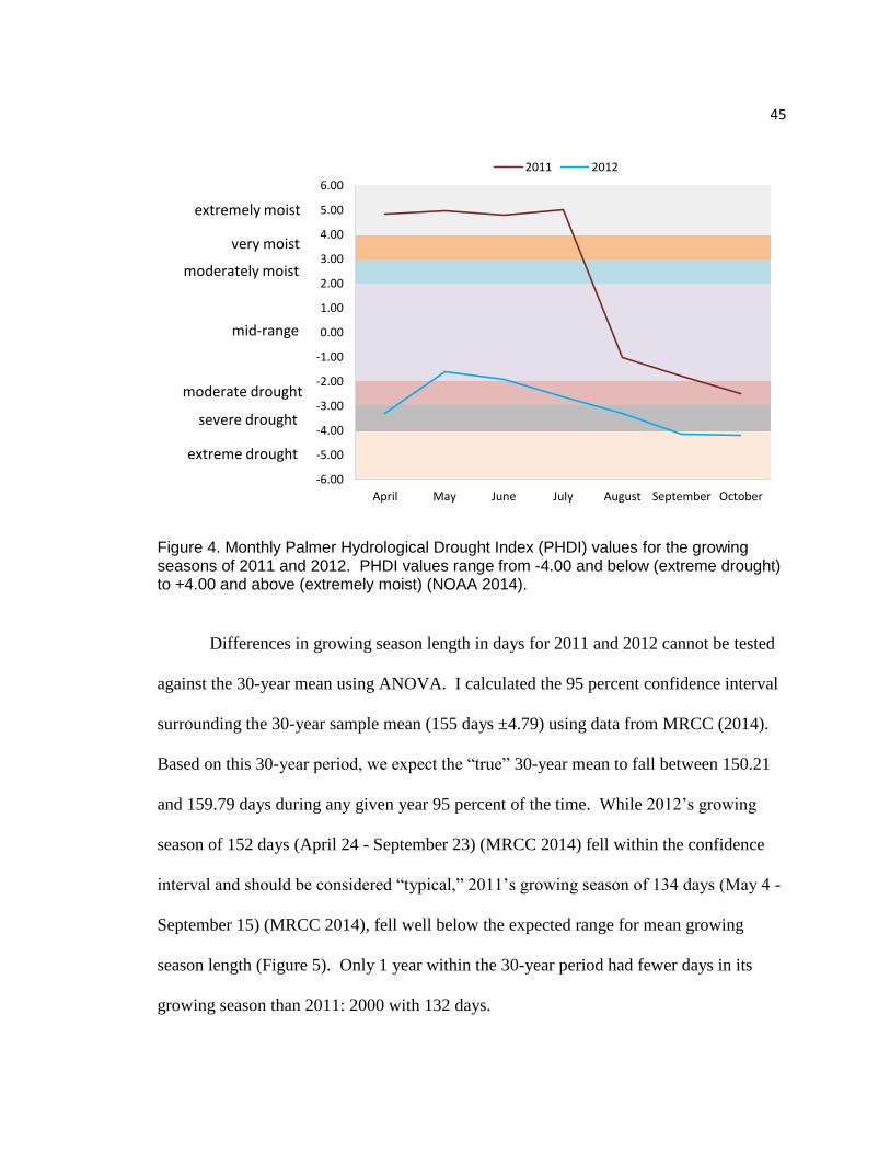
45

Figure 4. Monthly Palmer Hydrological Drought Index (PHDI) values for the growing seasons of 2011 and 2012. PHDI values range from -4.00 and below (extreme drought) to +4.00 and above (extremely moist) (NOAA 2014).

Differences in growing season length in days for 2011 and 2012 cannot be tested

against the 30-year mean using ANOVA. I calculated the 95 percent confidence interval

surrounding the 30-year sample mean (155 days ±4.79) using data from MRCC (2014).

Based on this 30-year period, we expect the “true” 30-year mean to fall between 150.21

and 159.79 days during any given year 95 percent of the time. While 2012’s growing

season of 152 days (April 24 - September 23) (MRCC 2014) fell within the confidence

interval and should be considered “typical,” 2011’s growing season of 134 days (May 4 -

September 15) (MRCC 2014), fell well below the expected range for mean growing

season length (Figure 5). Only 1 year within the 30-year period had fewer days in its

growing season than 2011: 2000 with 132 days.

-6.00

-5.00

-4.00

-3.00

-2.00

-1.00

0.00

1.00

2.00

3.00

4.00

5.00

6.00


2011 2012

extreme drought

severe drought

moderate drought

mid-range

moderately moist

very moist

extremely moist

46

Figure 5. Mean number of days in the growing season (April-October) for a 30-year period (1981-2010) shown by bar, error bar represents the 95% confidence interval surrounding the mean. Dots represent the number of days in the growing seasons of 2011 and 2012 (MRCC 2014).

2011 Walk-Through Method

The 2011 floristic survey utilizing the walk-through method yielded 112 different

species within 88 genera in 33 families (Table D1). Families represented by the most

species were Asteraceae (sunflower) with 28 percent, Poaceae (grass) with 12 percent,

Fabaceae (legume) with 9 percent, Cyperaceae (sedge) with 8 percent, and Lamiaceae

(mint) with 3.5 percent of species present. The most common genera in each of these

families are listed from more- to less-numerous, respectively, unless otherwise noted;

Asteraceae: goldenrod, aster, sunflower, and ragweed (sunflower and ragweed equal);

Poaceae: Kentucky and Canada bluegrass and brome (equal); Fabaceae: clover, vetch,

and sweet clover (vetch and sweet clover equal); Cyperaceae: sedge, bulrush, and

2011

2012

130

135

140

145

150

155

160

165

1981-2010 mean

Nu

mb

er

of D

ays in

Gro

win

g S

ea

so

n

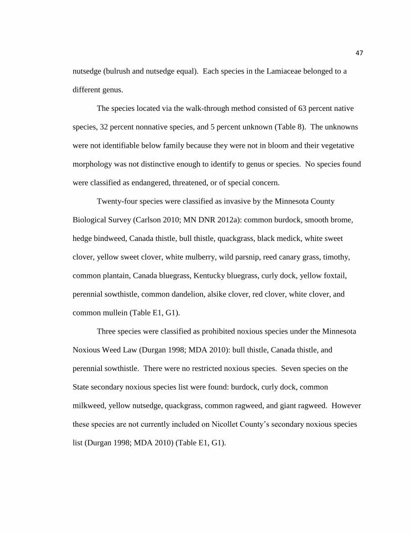
47

nutsedge (bulrush and nutsedge equal). Each species in the Lamiaceae belonged to a

different genus.

The species located via the walk-through method consisted of 63 percent native

species, 32 percent nonnative species, and 5 percent unknown (Table 8). The unknowns

were not identifiable below family because they were not in bloom and their vegetative

morphology was not distinctive enough to identify to genus or species. No species found

were classified as endangered, threatened, or of special concern.

Twenty-four species were classified as invasive by the Minnesota County

Biological Survey (Carlson 2010; MN DNR 2012a): common burdock, smooth brome,

hedge bindweed, Canada thistle, bull thistle, quackgrass, black medick, white sweet

clover, yellow sweet clover, white mulberry, wild parsnip, reed canary grass, timothy,

common plantain, Canada bluegrass, Kentucky bluegrass, curly dock, yellow foxtail,

perennial sowthistle, common dandelion, alsike clover, red clover, white clover, and

common mullein (Table E1, G1).

Three species were classified as prohibited noxious species under the Minnesota

Noxious Weed Law (Durgan 1998; MDA 2010): bull thistle, Canada thistle, and

perennial sowthistle. There were no restricted noxious species. Seven species on the

State secondary noxious species list were found: burdock, curly dock, common

milkweed, yellow nutsedge, quackgrass, common ragweed, and giant ragweed. However

these species are not currently included on Nicollet County’s secondary noxious species

list (Durgan 1998; MDA 2010) (Table E1, G1).

48

Four species were classified as Tier 1 Quality Indicators, according to the

Minnesota County Biological Survey Native Indicator Species List (Carlson 2010; MN

DNR 2012a): leadplant, common sneezeweed, prairie blazing star, and common golden

alexander. Five species were identified as Tier 2 Quality Indicators (Carlson 2010; MN

DNR 2012a): butterfly-weed, prairie heart-leaved aster, Indian grass, tall meadow rue,

and Culver's root.

Twelve species were indicators of high-quality prairies (Curtis 1971): common

water hemlock, Canadian tick-trefoil, northern bedstraw, sawtooth sunflower, prairie

coneflower, black-eyed Susan, Missouri goldenrod, gray goldenrod, prairie cord-grass,

tall meadow rue, Culver’s root, and common golden alexander.

Species diversity calculations using the Shannon-Wiener Index and the Simpson’s

Index of Diversity could not be calculated for 2011 because there were no species

abundance data. Species area curves, frequency, percent cover, and litter depth were also

not calculated since the walk-through method is not designed to gather these data.

Mean-C and FQI for the Oak Leaf Lake Unit were calculated using all taxa on the

site. An adjusted mean-C and FQI omitted the following species that are not expected to

occur on prairies: (1) deciduous forest species (sugar maple and green ash), (2) emergent

aquatic species (water lily, narrow-leaved cattail, and arrowhead), and (3) native species

not listed by Ladd (2005) or located at Kasota Prairie (water smartweed, white vervain,

white avens, orange jewelweed, common elder, prairie bulrush, catnip, arrow-leaved

aster, and beaked sedge). These indices are reported in Table 8.

49

2012 Random-Sampling Method

The 2012 floristic survey utilizing the random-sampling method yielded 57

different species within 50 genera within 24 families (Table D1). All 57 species were

located during the 2011 season using the walk-through method. Families represented by

the most species were Asteraceae (sunflower) with 32 percent, Poaceae (grass) with 17

percent, Apiaceae (carrot) with 5 percent, Cyperaceae (sedge) with 5 percent, Fabaceae

(legume) with 3 percent, Polygonaceae (smartweed) with 3 percent, and Salicaceae

(willow) with 3 percent of species. The most common genera in each of these families

are listed from more- to less-numerous, respectively, unless otherwise noted; Asteraceae:

goldenrod, aster, sunflower, ragweed, and thistle (aster, sunflower, ragweed, and thistle

equal); Poaceae: brome; Cyperaceae: bulrush and sedge. Each species in the Apiaceae

belonged to a different genus.

The species located via the random-sampling method comprised 63 percent native

species, 32 percent nonnative species, and 5 percent of unknown origin. The unknowns

were not identifiable below family because they were not in bloom and their vegetative

morphology was not distinctive enough to identify the species. No species found were

classified as endangered, threatened, or of special concern.

Thirteen species were classified as invasive by the Minnesota County Biological

Survey (Carlson 2010; MN DNR 2012a): common burdock, smooth brome, Canada

thistle, bull thistle, white mulberry, wild parsnip, reed canary grass, common plantain,

Kentucky bluegrass, curly dock, perennial sowthistle, common dandelion, and red clover.

50

Three species found were classified as prohibited noxious species under the

Minnesota Noxious Weed Law (Durgan 1998; MDA 2010): bull thistle, Canada thistle,

and perennial sowthistle. There were no restricted noxious species. Five plant species on

the State secondary noxious species list were found (Durgan 1998; MDA 2010): burdock,

curly dock, common milkweed, common ragweed, and giant ragweed. However these

species are not currently included on Nicollet County’s secondary noxious species list.

Two species were classified as Tier 1 Quality Indicators (Carlson 2010; MN DNR

2012a): common sneezeweed and common golden alexander. One species was classified

as a Tier 2 Quality Indicator: Indian grass (Carlson 2010; MN DNR 2012a). Seven

species were indicators of high-quality prairies (Curtis 1971): common water hemlock,

sawtooth sunflower, prairie coneflower, black-eyed Susan, gray goldenrod, prairie cord-

grass, and common golden alexander.

Shannon-Wiener Diversity Indices and Simpson’s Diversity Indices for the

random-sampling method are reported in Table 8.

The five most-frequently-occurring plant species were ranked for each of the

three sampling events and for the full season; rankings are reported in Table 5. The

random-sampling technique requires that all individuals be counted, therefore plants that

were not in bloom were identified to species using vegetative characters whenever

possible.

51

Table 5. Top five most frequently-occurring species for each sampling event (classified by blooming/fruiting periods I, II, and III) and for the full season during the 2012 growing season in randomly-located quadrats at the Oak Leaf Lake Unit (1 = the highest frequency; 5 = the lowest frequency).

Species I II III full season

smooth brome 1 2 1 1

wild bergamot 3 3 3 2

big bluestem 1 2 3

Kentucky bluegrass 2 4 4

sawtooth sunflower 5 4 5

common golden alexander 4

reed canary grass 5

Maximillian sunflower 5

Cover class data for cover categories collected during the random-sampling

method are given in Table 6.

Table 6. Mean cover class for each sampling event (classified by blooming/fruiting periods I, II, and III) and for the full season during the 2012 growing season in randomly-located quadrats at the Oak Leaf Lake Unit (Range is 1 – 6, with 1 = the lowest percentage of cover). “Other” includes rocks, logs, moss, etc.

Class/ Sampling event

bare ground

native grass

native forbs

nonnative grass

nonnative forbs

duff/ litter

other

I 2 2 2 3 2 2 1

II 1 3 2 3 1 1 1

III 1 3 3 3 2 1 1

Full Season 1 3 2 3 2 2 1

52

The mean litter depth was 2.6 cm for Period I (the early-blooming/fruiting), 2.1

cm for Period II (the mid-blooming/fruiting), and 1.9 cm for Period III (the late-

blooming/fruiting). The mean litter depth was 2.2 cm for the full season.

Mean-C using all values calculated for the full season was 3.9 and the original

FQI for the full season was 23.0. The adjusted mean-C for the full season was 4.0 and

the adjusted FQI for the full season was 22.1 (Table 8).

Distribution of Species within Three Site Sections (A, B, C)

Section A consists primarily of mesic grassland and disturbed areas including the

driveway, parking area, and boat access. Section B is transitional between mesic

grassland and wetlands, which take up most of Section C (Figure B1). Table 7 shows the

number and percent of species located during the 2011 and 2012 seasons using the walk-

through and random-sampling methods, respectively, for each section within the site.

More than one-third of the high-quality indicator species (MCBS Tier 1, MCBS

Tier 2, and/or sensu Curtis; Table G1) present at the study site were found in all three

sections (Table 12). Similar numbers of indicator species were found in each of the three

sections (A = 10, B = 12, and C = 11), with all but one indicator species found either only

in one section or in all three sections. Six upland indicator species were found, with one

(butterfly-weed) in Section A, one (gray goldenrod) in Section B, one (leadplant) in

Section C, one (prairie heart-leaved aster) in Sections A and B, and two (gray-headed

coneflower and Missouri goldenrod) in Sections A, B, and C. Three facultative upland

indicator species were found, with one (Canadian tick trefoil) located in Section A and

53

Table 7. Species located in Sections A, B, and C of the Oak Leaf Lake Unit during the walk-through method in 2011 (112 species) and the random-sampling method in 2012 (57 species).

# of species 2011 2012

# of species % of species # of species % of species

in A 42 38% 19 33%

in B 12 11% 4 7%

in C 17 15% 8 14%

in both A & B 6 5% 2 4%

in both A & C 0 0% 0 0%

in both B & C 8 7% 1 2%

in A, B, & C 27 24% 23 40%

two (Indian grass and black-eyed Susan) in Sections A, B, and C. Four facultative

indicator species were found, with three (prairie blazing star, Culver’s root, and northern

bedstraw) located in Section B and one (common golden alexander) in Sections A, B, and

C. Four facultative wetland indicator species were found, with two (purple meadow rue

and prairie cordgrass) located in Section C and two (common sneezeweed and sawtooth

sunflower) in Sections A, B, and C. The only obligate wetland indicator species

(common water hemlock) was located in Section C.

Most species were either present exclusively in one section (64 percent) or

occurred in all three sections (24 percent). More than one-third of the species located in

all three sections were native perennial forbs with mid-range C-values. All but one of the

early-successional species occurred in Section A (with over half found exclusively in

Section A), about one-fourth also occurred in Section B, and only one occurred in

Section C.

54

DISCUSSION

The primary objective of this study was to perform a floristic survey and to gather

baseline data for the Oak Leaf Lake Unit. This was accomplished during two growing

seasons using two methods: a walk-through method during 2011 and a random-sampling-

in-quadrats method during 2012. Data were used to assess the ecological quality of the

site by calculating diversity and quality indices, and using Jaccard’s indices to compare

the study site’s flora to that of other prairies in the region. Indices generated by the two

data collection methods were compared.

Flora at the Oak Leaf Lake Unit

The flora at the 20-year-old Oak Leaf Lake Unit is typical of Midwestern mesic to

wet prairies. The site is dominated by long-lived herbaceous perennials. Ladd (2005)

provides a list of 988 Midwestern tallgrass prairie species that he separates into

“physiognomic classes” based on habit and duration. These are ranked by percentage

with perennial forbs, annual and biennial forbs, and grasses (including all grasslike

species) making up about 52, 17, and 22 percent of species, respectively (Ladd 2005).

The same classes at the Oak Leaf Lake Unit comprise 49, 16, and 21 percent,

respectively. The three most important families are Asteraceae including species in

sunflower (genus Helianthus), aster (genus Symphyotrichum), and goldenrod (genus

Solidago), etc., Poaceae, including big bluestem, switchgrass, Indian grass, prairie cord

grass, etc., and Fabaceae, including lead plant, Canadian tickfoil, and American vetch

(Tables D1, E1).

55

Eight percent of species at the study site are tree species compared to 1.6 percent

of species on Ladd’s (2005) list. The study site is in the ecotone between prairie and

deciduous forest biomes so there is sufficient moisture to support tree species typically

found in forests including native Acer saccharum (sugar maple) and Fraxinus

pennsylvanica (green ash), and naturalized nonnatives Morus alba (white mulberry) and

Pyrus malus (crab apple), which are growing on the study site but are not typical of

prairies (Curtis 1971; Ladd 2005). The study site is close to stands of deciduous forest

that act as seed sources. Many tallgrass prairies are located farther away from the

deciduous forest biome and/or they are too dry to support these tree species (Curtis 1971;

Tester 1995; Kline 2005; Ladd 2005).

Of 112 species located on the site, at least 70 are native; 59 of these are prairie

species. Forty-seven prairie species found at the site have been assigned coefficients of

conservatism (C-values) between 1 and 10; such species factor into the calculation of

mean-C and FQI (Tables 10, D1, E1). Seventeen prairie species at the Oak Leaf Lake

Unit have C-values of 6 to 10, which indicates high quality; a C-value of 10 indicates a

species that almost always occurs on an undisturbed high-quality site (TNGPFQAP

2001). Species with C-values of 5 can usually be located in natural areas, but may also

be found in disturbed areas (TNGPFQAP 2001). Eighteen indicator species (Curtis 1971;

Carlson 2010; MN DNR 2012a) fill niches in mid- and late-successional stages of a

prairie (Tables E1, G1), which indicates the site is mature. Tier 1 high-quality indicators

leadplant and prairie blazing star are among the most sensitive or difficult to establish

species (Carlson 2010; MN DNR 2012a).

56

Because the site is in the ecotone between prairie and deciduous forest biomes,

high-quality indicators, such as sugar maple and green ash, with C-values of 10 and 5,

respectively, increase mean-C and the FQI for the site. These species’ C-values were

omitted from calculations of adjusted quality indices because they are indicators of high-

quality deciduous forests not prairies (Curtis 1971, Ladd 2005). With the site adjacent to

a lake, other high-quality indicators, such as water lily, with a C-value of 9, also increase

mean-C and the FQI for the site and were omitted from calculations of quality indices

because they are indicators of high-quality aquatic habitats not prairies (Curtis 1971,

Ladd 2005). TNGPFQAP (2001) lists other species not expected to be found in prairies

like orange jewelweed with a C-value of 4, which is usually found near woods or in damp

habitats. Such species, not listed by Ladd, and not found at Kasota Prairie were also

omitted from calculations of adjusted quality indices. The mean-C and FQI were

originally calculated for all species listed by TNGPFQAP (2001). Adjusted mean-C and

FQI were calculated omitting 14 non-prairie species (see p. 48). The adjusted mean-C

and FQI only include species that are adapted to and occur in prairie habitats so that the

site’s quality can be accurately assessed.

Some prairie species located at the study site were not assigned C-values by

TNGPFQAP (2001), which includes the flora of North and South Dakota. Ladd (2005)

provides C-values for species from other states’ lists, which allowed me to assign C-

values if they were missing. I used C-values from the Illinois list first, and if Illinois did

not list a species, I selected a C-value from the next closest state. For example, marsh

spikerush is a high-quality species found at the study site, but not assigned a C-value by

57

TNGPFQAP (2001). Illinois assigns it a C-value of 8, which may not be in perfect

accord with its perceived value in Minnesota, but it is better than omitting the species

altogether. Omitting high-quality prairie species from calculations of mean-C and FQI

will lead to an underestimate of the quality of the site.

A comparison of the FQI using all taxa and the adjusted FQIs brings to light the

problem of calculating these indices without carefully considering whether the species

present are typical representatives of the community of interest, in this case, a prairie.

Including such taxa may lead to an overestimation of the quality of the site. Although the

original mean-C and FQI calculated for the Oak Leaf Lake Unit are not much different

from the adjusted indices, the original FQI of 36.1 hovers at the very edge of being

inadequate (threshold = 35) in native species and biodiversity. The adjusted FQI of 32.2

gives a clearer signal that the quality of the site is low (Table 8). These results suggest

that caution should be taken to ensure the species included in mean-C and FQI are

typically found in the community of interest.

No rare or endangered species were located, but that does not mean rare or

endangered species do not occur at the study site. The walk-through method might have

turned up rare species if they had been in bloom and/or clearly visible during visits.

Some rare species have short blooming periods that may have occurred between visits or

before June 13 when the first visit was made. Given the constraints of the random-

sampling method, rare species would only be listed if they were present in a quadrat.

58

Early-Successional Species and Weeds

Species that fill early-successional niches are able to endure environmental

extremes such as high heat, lack of shade, and dry soil, which may have low organic

matter and nutrient content. Such conditions are common in disturbed areas. These

species cover bare ground, reducing erosion and eventually increasing soil organic

matter. They provide shade, thereby keeping soil cooler and reducing soil water loss,

which increases germination rates and seedling survival rates of mid- and late-

successional species. Foster and Tilman (2000) show that as the age of a prairie

increases, the species richness of annual and nonnative early-successional species

declines and the species richness of perennial native forb and grass species increases.

Of the 23 annual, biennial, to short-lived perennials that are generally considered

early-successional species found at the site, 16 are nonnative, 11 are classified as

invasive, and four are State Secondary Noxious species (Gleason and Cronquist 1991;

MDA 2010, 2012; University of Minnesota Extension 2015a, 2015b, 2015c) (Table G1).

Fourteen of these species are confined to Section A of the site where disturbed areas

along the driveway and boat launch are located (Table G1).

Four short-lived native species at the site, orange jewelweed, rough fleabane, tall

lettuce, and black-eyed Susan have C-values of 4, 3, 6, and 5, respectively. Orange

jewelweed was omitted from the adjusted FQI because it is commonly found in

woodlands and ditches. It is not included in Ladd’s (2005) list of prairie species. Rough

fleabane, tall lettuce, and black-eyed Susan are expected on prairies and their C-values

contribute to the site’s FQI. Other native annual species, common and giant ragweed,

59

and horseweed, are viewed as undesirable “weeds” in agricultural settings and gardens so

they receive C-values of 0. The ragweeds cause hay fever.

Of 24 species classified as invasive by MCBS (Carlson 2010; MN DNR 2012a)

and/or as prohibited noxious species (MDA 2010, 2012), and State secondary noxious

species (MDA 2010, 2012), all but three species, (common and giant ragweed, and

common milkweed) are nonnative (Table G1). Of these, 11 are short-lived, early-

successional species. Perennial invasive/noxious species, including reed canary grass,

hedge bindweed, yellow sweet clover, white sweet clover, and Canada thistle (Table G1)

may threaten the long-term quality of the site. Invasive perennials have the potential to

outcompete and replace native species and disrupt entire communities, which decreases

plant biodiversity and the overall quality of prairies. The strong presence of native

perennial species at the site is encouraging because they will resist displacement by

invasive species better than annuals and short-lived perennials (Foster and Tilman 2000).

Although common milkweed is listed as a State secondary noxious species,

perhaps because it spreads very aggressively by runners, it is native and an integral part

of the community as a larval host and specialized species for pollinators such as Danaus

plexippus (monarch butterfly) (Kevan et al. 1989). Propagation of common milkweed is

now encouraged, mostly in landscape and horticulture settings, to increase declining

monarch butterfly populations. Monarch butterflies lay their eggs on common milkweed

so that larval stages can feed on the plant and take up secondary compounds that protect

the plant from insect herbivores; these, in turn, make monarch caterpillars repulsive to

their predators (USDA 2012c).

60

Assessing the Site’s Diversity and Quality

Because two floristic data sets were collected using two different methods during

the 2011 and 2012 growing seasons, two sets of indicators and indices of diversity, and

quality were calculated for the two full seasons. Each season was also broken into early-,

mid-, and late-blooming/fruiting periods for which indices were calculated. Table 8

summarizes these data.

Table 8 (on next page). Summary of floristic data collected at the Oak Leaf Lake Unit with quality-assessment indices mean-C and FQI derived from them for entities located by two methods (WT = walk-through in 2011 and R = random-sampling in 2012) for the full season and for three blooming/fruiting periods. Jaccard’s coefficients (Cj) indicate similarity of entities located by WT and R methods. “Total # unique to the year” refers to the number of species that were only found in the year indicated. Shannon-Wiener Diversity Indices (H) and Simpson’s Index of Diversity (D) were calculated for each of the three blooming/fruiting periods and the full season. The usual range of H is 1.5 to 3.5, with species diversity increasing as H increases. D ranges from zero to one, with diversity increasing as D increases.

61

Table 8. Summary of floristic data collected at the Oak Leaf Lake Unit by two methods (WT = walk-through in 2011 and R = random-sampling in 2012) for the full season and for three blooming/fruiting periods. Full caption on previous page. I II III Full Season

WT R

WT R

WT R

WT R

# sampling of events 4 1 5 1 4 1 13 3

# families 16 16

16 7

16 6

33 24

% families 48% 67%

48% 29%

48% 25%

100% 100%

# species located for first time 41 44

40 7

31 6

112 57

% species 37% 77%

36% 12%

28% 11%

100% 100%

# native 20 25

28 6

22 5

70 36

% native of total species located 18% 44%

25% 10%

20% 9%

63% 63%

# nonnative 20 16

11 1

5 1

36 18

% nonnative of total species located 18% 28%

10% 2%

4% 2%

32% 32%

# unknown 1 3

1 0

4 0

6 3

% unknown of total species located 1% 5%

1% 0%

3% 0%

5% 5%

total # species unique to year - - - - - - 55 0

# MCBS indicator species 2 2

4 0

3 1

9 3

# Curtis indicator species 5 6

5 0

2 1

12 7

# invasive species 14 11 7 2 3 0 24 13

# MDA noxious species 3 7

5 1

2 0

10 8

# other weed species 10 7

6 1

1 0

17 8

# of early-successional species 11 7 11 5 1 1 23 13

original mean-C 4.1 3.7 4.6 4.3 4.5 4.3 4.4 3.9

adjusted mean-C 4.5 3.9 4.6 3.7 3.9 4.4 4.3 4.0

original FQI 17.0 18.6 24.4 8.5 20.5 10.6 36.1 23.0

adjusted FQI 17.3 18.8 21.5 6.4 16.7 9.8 32.2 22.1

H - 3.0 - 2.7 - 2.6 - 2.3

D - 0.923 - 0.905 - 0.903 - 0.924

Cj 0.25 0.07 0.03 0.51

62

In every measure and index (except diversity indices, H and D, which cannot be

calculated using 2011 data), the walk-through method yielded a value indicating greater

richness and quality. Because a flora consisting largely of herbaceous perennials is not

expected to change much from season to season, the overall quality of Oak Leaf Lake

Unit’s flora will be discussed using data derived from the 2011 walk-through method. A

comparison, including strengths and weaknesses of the two data collection methods, will

be made and discussed below.

To further assess the diversity and quality of the flora of the Oak Leaf Lake Unit,

I calculated Jaccard’s coefficients to compare its flora with floras at 11 predominantly-

grassland sites. Schiebout et al. (2008) concluded that locations closer to each other have

more similar taxa, so the 11 sites were chosen for their proximity to my site. Species lists

for the sites came from Kramer (1975) and MN DNR (2016b). Table 9 reports Jaccard’s

coefficients, proximity, number of similar habitats, adjusted mean-C, and adjusted FQI

for the 12 sites. As predicted by Schiebout et al. (2008), sites closest to the study site had

the highest Jaccard’s coefficients, although none of the coefficients indicated very high

similarity. Oak Leaf Lake’s flora is most similar to that of the Kasota Prairie, a 42-acre

site made up of native mesic/tallgrass prairie and restored prairie after grazing. Kasota

Prairie’s FQI of 65.3 indicates it is a very high-quality site. The two sites are closest to

each other and have the greatest number of similar habitats and elevation. For these

reasons, Kasota Prairie was chosen as a representative site of a high-quality prairie to

compare to the study site. It is important to point out that the species list from Kasota

63

Prairie is more than 40 years old; species composition and richness may have changed

over the years.

Although nearby Rasmussen Woods has a similar flora based on Jaccard’s

coefficient, it was not chosen because Rasmussen has a large deciduous forest component

with many woodland species and its grassland species are not indicative of high-quality

prairies. The other sites were not chosen because they were too far away from the study

site, shared lower species similarities based on Jaccard’s coefficients, and/or had too few

habitats in common.

Table 9. Jaccard’s coefficients (Cj) comparing the flora of the Oak Leaf Lake Unit with floras of 11 predominantly-grassland sites within Minnesota (10 are MN DNR scientific and natural areas [SNAs]) ranked from highest to lowest similarities. Their proximity and number of similar habitats to the Oak Leaf Lake Unit are also listed. The mean C-value and floristic quality index (FQI) were also calculated for each site.

Cj with Oak Leaf Lake

Unit

proximity to Oak

Leaf Lake Unit (km)

# of habitats similar to Oak Leaf Lake Unit

adjusted

C

adjusted FQI

Oak Leaf Lake Unit - - - 4.3 32.2

Kasota Prairie SNA 0.20 5 3 5.3 65.3

Rasmussen Woods Nature Area 0.18 19 3 4.7 52.4

Cottonwood River Prairie SNA 0.17 90 3 5.3 55.0

Cedar Mountain SNA 0.14 72 3 5.6 67.4

Rock Ridge Prairie SNA 0.13 89 1 5.7 51.0

Joseph A. Tauer Prairie SNA 0.12 45 2 6.0 41.7

Osmundson Prairie SNA 0.12 97 1 5.8 35.5

Yellow Bank Hills SNA 0.11 240 1 5.3 39.4

Clinton Prairie SNA 0.08 241 2 5.9 34.7

Bonanza Prairie SNA 0.06 258 2 6.2 47.6

Blue Devil Valley SNA 0.01 137 1 4.1 14.7

64

Species Richness

Although floras at the study site and Kasota Prairie had the greatest Cj value, 0.20

does not indicate high similarity. The Oak Leaf Lake Unit supports 112 different species

of which, 63 percent are native. Kasota Prairie supports 187 different species, of which

82 percent are native. The Kasota Prairie site is remnant native prairie that was

established as an SNA in 1984, while the Oak Leaf Lake Unit was once agricultural land

restored to prairie in 1994. Because Kasota Prairie has not been disturbed much since

presettlement times it is more likely to have greater species richness including many

more sensitive and late-successional native species, like rattlesnake master, a facultative

wetland species with a C-value of 8 (Ladd 2005), which is found at Kasota Prairie, but

not at the study site (Kramer 1975). The sites do share some high-quality indicator

species, such as leadplant, Indian grass, and Culver’s root. Both sites also have

invasive/noxious species in common, such as reed canary grass, Canada thistle, and

yellow and white sweet clover.

Table 10 summarizes moisture requirements for native species in two classes,

sensitive species with C-values between 6 and 10 and less sensitive species with C-values

between 1 and 5, for the Oak Leaf Lake Unit and Kasota Prairie. While 38 percent of

Kasota Prairie’s 103 native species are adapted to dry uplands, only 13 percent of Oak

Leaf Lake’s 47 native species are (Table 10). In contrast, Oak Leaf Lake has two high-

quality obligate wetland species, while Kasota only has one. This suggests that Kasota

Prairie has drier habitats to support obligate upland species. Ladd’s (2005) data show

that nearly half of prairie species are adapted to dry upland habitats that are found across

65

the Great Plains. Kasota Prairie and the study site share nine obligate upland species

including Amorpha canescens (leadplant), and Ascelepias tuberosa (butterfly weed).

However Kasota Prairie is home to 47 additional obligate upland species not found at the

Oak Leaf Lake site, including Anemone patens (pasqueflower), Bouteloua curtipendula

(side-oats grama), and Petalostemon purpureum (purple prairie clover).

Mean C-values and floristic quality index (FQI) at Oak Leaf Lake and Kasota

Prairie differed. The Oak Leaf Lake Unit’s mean-C value was 4.3 and the FQI was 32.2.

The Kasota Prairie’s mean-C value was 5.3 and the FQI was 65.3 (Table 9). Kasota

Prairie’s higher mean-C can be attributed to it having a higher percentage of late-

successional high-quality native species than the Oak Leaf Lake Unit. Fifty-nine percent

of Kasota Prairie’s native species have C-values of 6 to 10 compared to 36 percent of

Oak Leaf Lake’s species in the same category (Table 10). The large differences between

the FQIs for the two sites is also due to the difference in numbers of native species at the

sites. Kasota Prairie has 103 native species compared to 47 at the Oak Leaf Lake Unit.

The adjusted FQI for the study site indicates it has an insufficient number of native

species and inadequate biodiversity (Swink and Wilhelm 1994; Higgins et al. 2001). An

increase in invasive species could suppress native species and decrease the FQI at the

Oak Leaf Lake Unit even further. Loss of plant diversity would mean fewer pollinating

bees and butterflies, fewer insects for birds and their young to feed on, and fewer

animals, such as mice, voles, fox, snakes, gophers, and deer, essential to the food web.

66

Table 10. Species at Oak Leaf Lake Unit and Kasota Prairie SNA with C-values between 1 and 10 organized into wetland rating classes per the Army Corps' wetland classification system (Lichvar et al. 2014) with Ladd's (2005) numerical classification in parentheses.

Oak Leaf Lake Unit Kasota Prairie SNA

Wetland class

Spp in

class

C-values6 to 10

% in class

C-values 1 to 5

% in class

Spp in

class

C-values 6 to 10

% in class

C-values 1 to 5

% in class

UPL (5) 12 6 12.8 6 12.8 52 39 37.9 13 12.6 FACU (4 to 1) 13 4 8.5 8 17.0 23 11 10.7 12 11.7

FAC (0) 3 2 4.3 1 2.1 4 2 1.9 2 1.9 FACW (-1 to -4) 11 3 6.4 7 14.9 18 9 8.7 9 8.7

OBL (5) 8 2 4.3 6 12.8 6 1 1.0 5 4.9

Total 47 17 36.2 28 59.6 103 62 59.2 41 35.0

Species Diversity

Shannon-Wiener and Simpson’s Diversity Indices can only be calculated when

species abundance data are available, therefore they are derived from 2012 data. Both

indices are measures of species diversity, with the Shannon-Wiener Index measuring

species richness and evenness and the Simpson’s Index of Diversity placing more weight

on species abundance than on species richness. It is important to note that the Shannon-

Wiener and Simpson’s Diversity Indices calculated for the site only included 57 out of

the 112 species identified at the site.

The Shannon-Wiener Diversity Index for the full season is close to the midpoint

indicating “medium” diversity for the site (Table 8). The Simpson’s Index values

indicate overall high diversity at the study site (Table 8). Although the indices show

medium to high levels of diversity at the Oak Leaf Lake Unit, they do not take into

67

account the quality of the species. The species used in the calculation of these diversity

indices included more than half of the low-quality species at the site, including 13

invasive species. This is a weakness of these indices: diversity can appear to be adequate

or high, but this does not tell the whole story. Without knowing what species are present,

there is no way to judge the quality of the site. This also highlights a risk of the random-

sampling method, which is failure to capture all species present at a site. When species

are not included, diversity is underestimated. Furthermore, species that fall outside

quadrats may be rare. Rare species are often indicators of high quality sites. Failure to

take them into account may cause an investigator to overlook a critically important site.

Greater high-quality species diversity is ecologically important because complex

communities are more stable (Foster and Tilman 2000). They provide more ecological

niches and more complex food webs. Diverse communities are resilient; they are better

able to adapt and thrive in response to environmental changes.

My data indicate that grasses made up a higher percentage of cover than forbs at

the Oak Leaf Lake Unit (Table 6). Although grasses are more common on the study site

(cover class 3/6), forbs were not scarce (cover class 2/6). Forbs represented a majority of

the total species located (65 percent), contributing importantly to the diversity of the site.

However, a lack of forbs is a concern in restored prairies (Volkert 1992; Sample and

Mossman 1997) because they are essential for nesting and brooding structures for some

bird species (Volkert 1992; Sample and Mossman 1997) and are the primary habitats for

many invertebrates, which in turn are an important food source for grassland birds and

their broods (Buchanan et al. 2006). Competition from established grasses can suppress

68

forb establishment. Baer et al. (2002) found that grasses accounted for less than 10

percent of total plant cover in restored grasslands that were four or fewer years old;

however, by year six, grasses made up more than 80 percent of total plant cover and forbs

were scarce. Camill et al. (2004) found a similar pattern and concluded species richness

was lower on restored grasslands than on undisturbed prairies because of the dominance

of grasses.

Comparison of Three Sections Within the Site

The Oak Leaf Lake Unit gradually slopes from mesic to wetland with a disturbed

area at the higher edge. The site is divided into three roughly-equal-sized sections:

Section A consists primarily of mesic grassland and disturbed areas, Section B is

transitional between mesic grassland and wetlands, which take up most of Section C

(Figure B1).

Indicator species were located in each section; finding indicator species in all

three sections suggests that the entire site offers high-quality species the conditions they

need to flourish. The number of early-successional species decreased from Section A

(with over half found exclusively in Section A) to Section B to Section C. This reflects

the gradient from disturbed through undisturbed mesic to more restrictive wetland

habitats at the site.

Section A had the greatest species richness, which is expected; this section

contains the widest variety of habitats including a disturbed area that is open to early-

successional species, including annuals and short-lived species (Tables 7, D1). More

69

than one-third of the species found exclusively in Section A are native perennial forbs

with C-values from 1 to 9, indicating a highly-variable assemblage that reflects the

patchiness of habitats in this section. Of 24 invasive species on the site, exactly half of

them were located exclusively in Section A and 11 of those are early-successional species

such as clover species, dandelion, and common plantain. Few early-successional

invasive species were located in Sections B and C, most likely because the sections’

relatively dense established vegetation does not provide the open conditions these species

thrive in. Even the ubiquitous common dandelion was found much less abundantly in

Sections B and C. Perennial invasive species such as Canada thistle, perennial sow-

thistle, and reed canary grass are found throughout the site; like native herbaceous

perennials, they may favor more stable conditions. A substantial stand of reed canary

grass is found in Section C. This aggressive invasive species prefers mesic to wet soils; it

is likely crowding out the native species while preventing or deterring the establishment

of any new species, including other invasive species.

Species differ in their ability to thrive in dry to wet substrates and their moisture

requirements and distributions can provide information about habitat conditions on a site.

Table 11 summarizes the moisture preferences and locations within the site (Sections A,

B, and C) for all species at the Oak Leaf Lake Unit. Table 12 summarizes the moisture

preferences and locations of high-quality indicator species at the site.

70

Table 11. Moisture preference for all species located in each section of the Oak Leaf Lake Unit according to the United States Army Corps of Engineers Region 3 Midwest 2014 Wetland Plant List (Lichvar et al. 2014) and Ladd’s (2005) coefficient of wetness (5 to -5, with 5 being the driest and -5 being the wettest) are obligate wetland (OBL = -5, almost always found in wetlands), facultative wetland (FACW = -1 to -4, usually found in wetlands, but may occur in non-wetlands), facultative (FAC = 0, found in wetland and non-wetlands), facultative upland (FACU = 1 to 4, usually found in non-wetlands, but occur in wetlands), and obligate upland (UPL = 5, almost never found in wetlands).

Section Wetland Code for All Species

OBL FACW FAC FACU UPL

unknown/ not listed

in A 3 5 8 14 4 8

in B 1 1 3 3 1 3

in C 4 3 2 2 2 4

in both A & B 0 1 0 3 1 1

in both A & C 0 0 0 0 0 0

in both B & C 2 1 0 1 0 4

in A, B, & C 1 4 5 12 3 2

Table 12. Moisture preference for indicator species located in each section of the Oak Leaf Lake Unit according to the United States Army Corps of Engineers Region 3 Midwest 2014 Wetland Plant List (Lichvar et al. 2014) and Ladd’s (2005) coefficient of wetness (5 to -5, with 5 being the driest and -5 being the wettest) are obligate wetland (OBL = -5, almost always found in wetlands), facultative wetland (FACW = -1 to -4, usually found in wetlands, but may occur in non-wetlands), facultative (FAC = 0, found in wetland and non-wetlands), facultative upland (FACU = 1 to 4, usually found in non-wetlands, but occur in wetlands), and obligate upland (UPL = 5, almost never found in wetlands).

Section Wetland Code for High-Quality Indicator Species

OBL FACW FAC FACU UPL

in A 0 0 0 1 1

in B 0 0 3 0 1

in C 1 2 0 0 1

in both A & B 0 0 0 0 1

in both A & C 0 0 0 0 0

in both B & C 0 0 0 0 0

in A, B, & C 0 2 1 2 2

71

Butterfly-weed and Canadian tick-trefoil are two high-quality indicator species

(MCBS Tier 1, Tier 2 and/or sensu Curtis) found exclusively in Section A (Table G1).

The former is an upland species and the latter a facultative upland species (Tables 12, D1,

E1, G1). Indicator species found exclusively in Section B were upland species gray

goldenrod and facultative species prairie blazing star, Culver’s root, and northern

bedstraw. Indicator species found exclusively in Section C were upland species

leadplant, facultative wetland species purple meadow rue and prairie cordgrass, and

obligate species common water hemlock. The occurrence of these species generally

reflects the gradient from higher to lower elevation and the moisture gradient from mesic

in Section A and wet-mesic to wet in Section C. All of the soil types at the study site

have high available water capacity, are poorly drained, and are in close proximity to a

lake, and therefore are probably most often mesic, wet-mesic, and/or wet. Half of Kasota

Prairie’s native species with C-values of 1-9 are obligate upland species while only a

quarter of the species at the Oak Leaf Lake Unit are in this class (Tables 10 and 11). If

the study site had true dry upland areas, we would expect to find more upland species like

those found at Kasota Prairie; instead the study site has more facultative species, such as

Culver’s root, common golden alexander, northern bedstraw, and prairie blazing star,

facultative wetland species such as sawtooth sunflower, common sneezeweed, prairie

cordgrass, and tall meadow rue, and obligate wetland species, such as common water

hemlock, swamp milkweed, and Bebb’s sedge (Curtis 1955).

72

Effects of Weather and Climate on the Flora at the Oak Leaf Lake Unit

Using data from MRCC (2014), I found that mean daily precipitation for August,

September, and October 2011 and June through September 2012 were significantly lower

than the 30-year (1981-2010) means for those months (Figure 2). Mean daily

temperatures for July 2011 and May, July, and October 2012 were significantly higher

than the 30-year (1981-2010) means for those months (Figure 3). Higher temperatures

and drought conditions during my survey years may be indicative of climate change in

our region, which may have long-term consequences for the site.

Foster and Tilman (2000) found a decline in species richness in their grassland

test plots by an average of 37 percent during drought conditions in 1988 through the

elimination of scarce annual species and rare species. Seventy-two percent of

Midwestern tallgrass species consist of herbaceous perennials; only 16 percent of species

are annuals (Ladd 2005). In general, common herbaceous perennial species will not be

lost during one season of drought because they survive winter by storing carbohydrates in

perennating organs such as rhizomes and storage roots (Raven et al. 2005). When new

shoots emerge in the spring, they are relying on energy stored the previous year (Raven et

al. 2005). The stature and vigor of individuals may be affected by dry years, but it will

likely take a series of very dry years before these tough, resilient species are killed. Rare

perennial species may be less tolerant of environmental extremes. Annual species

complete their life cycles in a single growing season. If it is too dry, seeds may not

germinate and seedlings and/or plants may not survive to produce seeds. Rare annual

species are particularly vulnerable. Tilman and Haddi (1992) suggest the loss of rare

73

species, due to increased drought frequencies as a result of climate change, is a threat to

biodiversity. The Oak Leaf Lake Unit flora consists of 82 percent perennial forbs and

grasses; its annual species are not rare, nor are most high quality indicators. Although the

drought conditions from July to October of 2012 were severe, they likely did not decrease

species richness at the site because perennial forbs and grasses are less likely to be lost to

short-term drought conditions, especially when they are abundant (Tilman and Haddi

1992).

In 2011 big bluestem plants were about 0.9-1.2 m tall, but in 2012 averaged about 1.4

m, with some as tall as 1.8 m. Big bluestem may be at or near maturity in some portions

of the site because the maximum height of big bluestem at maturity (approximately 20

years) is about 1.8 m tall. During 2012, big bluestem was patchy and mixed with smooth

brome, which was shorter than it was the previous year, averaging about 15 cm high. Big

bluestem is a facultative species (Lichvar et al. 2014), meaning it can occur in wetlands

and non-wetlands. The root systems of native prairie grasses like big bluestem are

generally much larger than those of nonnative grasses reflecting their adaptation to the

relatively dry prairies of the Great Plains. The roots of big bluestem can reach nine feet

deep and can access water and nutrients unavailable to shorter-rooted nonnative species,

such as smooth brome, with root systems only about one foot deep (MN DNR 2016c).

The big bluestem plants may have tolerated drought conditions during 2012 better than

the nonnative smooth brome on the site. However, the stand of invasive reed canary

grass in Section C expanded from 2011 to 2012.

74

I noticed more patches of native perennial forbs in 2012 than I did in 2011,

especially of sawtooth sunflower, Canada goldenrod, wild bergamot, and Maximillian

sunflower. The one patch of Carolina rose had become larger. There were fewer early-

successional species, black-eyed Susan and wild parsnip individuals in 2012 than in

2011. These short-lived species may suffer more than perennials during drought years.

Comparison of Data Collection Methods

Assessing the diversity of the study site using data collected in 2011 (walk-

through method) and 2012 (random-sampling method) yielded different results (Table 8).

Of the 112 unique species located on the site in 2011, only about half of them were

relocated using the random-sampling method in 2012 (Table 8). No new unique species

were located in 2012 (Table 8). While a greater number of invasive species, MDA

noxious species, and other undesirable species were located by the walk-through method,

they were balanced by increased numbers of high-quality MCBS and Curtis indicator

species. My study indicates that mean-C and FQI indices derived from walk-through

data will provide a more accurate assessment of the quality of the site because they are

based on species richness. Using data gathered by the random-sampling method will

seriously underestimate these quality indicators (Table 8).

Choosing the Best Sampling Method and Time to Collect Data

A thorough walk-through requires frequent visits to a site so that species with

short blooming or other reproductive periods will be noted and included in the flora.

75

Random-sampling using quadrats is also time consuming because individual plants must

be counted and measured within their quadrats.

The early-blooming/fruiting period (Period I) yielded the greatest species richness

for both the walk-through and random-sampling methods with fewer new species being

discovered during subsequent periods. Because identification of flowering plants relies

heavily on characters of flowers, the collection dates for species at the Oak Leaf Lake

Unit roughly correspond to the beginning of species’ blooming periods, especially for

data collected in 2011. Prairie species in Minnesota begin to bloom in mid April (Kramer

1975) so my Period I captured a 12-week blooming window, which is twice the length of

either Period II (five weeks) or Period III (six weeks). This might explain, in part, why

the first blooming period yielded more species. It should be noted, however, that prairie

species tend to bloom later in the season than herbaceous woodland species. Kramer

(1975) only lists four species at Kasota Prairie that bloomed before the end of May so it

is unlikely that I missed many, if any species by starting my surveys in early to mid June.

Kramer’s (1975) blooming calendar indicates 57 of the 111 species he observed

(51 percent) came into bloom between May 23 and July 9, which is roughly equivalent to

my Period I. I captured 37 and 77 percent of species at the Oak Leaf Lake Unit during

2011 and 2012 during Period I, respectively (Table 8). These percentages are quite

different from each other with Kramer’s (1975) observation at Kasota Prairie falling

about half-way between them. Early spring temperatures during 2011 and 2012 may

explain these discrepancies. Although the differences are not significant, mean daily

temperatures for April and May of 2011 were about 1° C cooler than the 30-year means

76

(Table 4, Figure 3). The growing season in 2011 was unusually short, lasting only 135

days as compared to the 30-year mean of 158 days (Figure 5); the last spring frost on

May 4th was six days later than the 30-year mean of April 29 (MRCC 2014). That only

37 percent of species were located within Period I in 2011 may, in part, be explained by

colder spring temperatures. Early-blooming species are very sensitive to warmer or

cooler temperatures, blooming one to two weeks earlier or later, respectively (A.

Mahoney, personal communication, March 20, 2016). During 2012, the mean daily

temperature for April was 1° C warmer than the 30-year mean and May was statistically

significantly warmer than the 30-year mean (Table 4, Figure 3). This may explain why

77 percent of species were noted in Period I in 2012.

Blooming periods at Kasota Prairie (Kramer 1975) show the same pattern I

observed at the Oak Leaf Lake Unit: fewer “new” species (as represented by species

coming into bloom) were discovered as the season progressed. Thirty-five percent of

species at Kasota came into bloom during my Period II and 20 percent came into bloom

during my Period III as compared to 35 and 12 percent of species at the Oak Leaf Lake

Unit in Period II and 28 and 11 percent in Period III for 2011 and 2012, respectively.

Despite the fact that Period I had the greatest species diversity, I conclude that if only one

visit per growing season could be performed, it should occur later in the season because

blooming seasons can last quite a while. Kramer’s (1975) calendar indicates that of 74

species that came into bloom in mid June, 30 (41 percent) were still in bloom by mid

August and 17 (23 percent) were still in bloom during the first week of September. Even

77

if some species are past their blooming/fruiting periods, dried flowers or fruits on the

plants often allow them to be identified.

My experiences suggest that choosing between the walk-through or random-

sampling methods is dependent upon the purpose of the study. If one is attempting to

create a flora for a relatively small area or if one is searching for rare species, or

observing habitat heterogeneity, the walk-through method may be preferable. If one is

looking for a “snapshot” of the overall characteristics of the vegetation, quantitative data

for statistical analyses, or the area is large, random-sampling in quadrats is preferred.

CONCLUSION

The primary objective of this study was to perform a floristic survey and to gather

baseline data for the restored prairie at Oak Leaf Lake Unit. This was accomplished

during two growing seasons using two methods: a walk-through method during 2011 and

a random-sampling-in-quadrats method during 2012. The secondary objective was to

assess the ecological quality of the site by comparing species richness, mean-Cs, and

FQIs with other prairies in the region.

My first null hypothesis, that species richness and FQI for the study site will not

differ from the species richness and FQI of other prairies in the region, is rejected. My

alternative hypothesis, that the study site has lower species richness and FQI than other

prairies in the region, is also rejected. The Oak Leaf Lake Unit had greater total species

richness than seven out of the 11 predominantly-grassland sites it was compared to. The

78

site had the third highest species-to-acres ratio out of the 12 sites. FQI for the Oak Leaf

Lake Unit was higher than one of the other 11 sites. One factor leading to greater species

richness but lower FQI may be the presence of disturbed areas in Section A, which

provide niches for early-successional species with low C-values. These species will drive

down an FQI in comparison to FQIs of less-disturbed mature sites with greater

proportions of higher-quality native species.

The Oak Leaf Lake Unit supports many fewer high-quality prairie species than

the Kasota Prairie, which also contributes to its inadequate FQI. Ladd (2005) shows that

58 percent of tallgrass prairie flora is adapted to dry upland habitats that characterize the

prairie biome across most of the Great Plains. Only 14 percent of prairie species listed by

Ladd (2005) occur in wetlands. Wet prairie areas are often calcareous fens or other

highly-specialized habitats that support assemblages of rare species adapted to such

conditions. Prairies in south central Minnesota where the Oak Leaf Lake Unit is located

must usually be maintained by fire because annual precipitation is sufficient for

succession to a climax deciduous forest. Although the Oak Leaf Lake Unit has been

managed as prairie since 1994, it’s moisture-retaining soils and annual precipitation allow

woodland species such as sugar maple, green ash, orange jewelweed, white avens, and

common elder to thrive.

While there are many naturally-occurring sources of woodland species seeds near

the Oak Leaf Lake Unit, among them a small woodlot immediately to the east of Section

C at the site (Figure A2), there are no close naturally-occurring sources of prairie species

seeds. Kasota Prairie is 5 km away across the Minnesota River to the east of the site. It

79

is highly unlikely that seeds from Kasota Prairie could buck the westerly winds and find

their way to the Oak Leaf Lake Unit. Furthermore, many high-quality prairie species are

adapted to dry upland soils; even if they were seeded at the site, conditions may not favor

germination and/or seeding survival. Transplants may also fail to thrive. Prairie species

adapted to dry uplands may be less able to compete with species adapted to mesic or wet

soils. Environmental conditions at the Oak Leaf Lake may always preclude the

establishment of the highest-quality upland prairie species.

My second null hypothesis, that species richness, as determined by the walk-

through method, will not differ from species richness as determined by the random-

sampling-in-quadrats method, is rejected. My alternative hypothesis, that the walk-

through sampling method will generate greater species richness than the random-

sampling-in-quadrats method, is supported with caution.

I found that a series of walk-throughs carried out during a full growing season

will likely yield a more comprehensive plant species list because this method, in

principal, allows an investigator the opportunity to locate “all” the species present at a

site, including rare species and/or any species that are not listed because they occurred

outside random sampling quadrats. That being said, if visits to a site are not carried out

often enough, some species may flower between visits and go unnoticed. An investigator

may not cover the entire area thoroughly, missing rare species. Basing a species list on a

single season may also lead to omissions. For instance, extreme weather conditions may

affect annual species (i.e. poor seed germination, poor seedling survival, small stature,

failure to produce many or any flowers). Annual species that perform poorly during one

80

year will likely produce fewer fruits and seeds, which could lead to a smaller population

the following year. Herbaceous perennials may also be affected by extreme weather.

The highest-quality indicators are sensitive to environmental conditions, and only thrive

in sites that reliably provide those conditions. Sensitive perennial species may perform

poorly (i.e., small stature, failure to produce many or any flowers). Small individuals that

fail to flower may be overlooked using the walk-through method.

I accept my alternative hypothesis with caution because I did not test both

sampling methods during the same year, which means that I cannot be absolutely certain

that I would find the same species using the two methods. However, I located nearly

twice as many species using the walk-through method in the same area that is mostly

populated by herbaceous perennial species. Studies show that differences in weather

(particularly drought) during different years do not substantially affect the presence of

perennial species (Tilman and Haddi 1992).

Random-sampling-in-quadrats techniques are generally used to study

“vegetation” on a site, i.e. “grassland,” or “deciduous woodland.” Strengths of this

method include collecting abundance data that can be used to calculate diversity indices,

like Shannon-Wiener and Simpson, and other quantitative data, including frequency,

percent cover, and litter depth, which can provide statistical analyses and valuable insight

into the overall characteristics and environmental conditions of the vegetation.

Vegetative studies tend to “simplify” vegetation into homogeneous sections, when

in fact, much more heterogeneity often exists. Floristic studies can reveal heterogeneity

but cannot assess abundance or distribution. Ideally, we should use floristic surveys

81

hand-in-hand with random-sampling surveys to get a better understanding of the

ecological quality of the grasslands. Tansley and Chipp (1926) wrote that “one can

acquire a considerable floristic knowledge and yet know next to nothing about

vegetation.” The same can be said about vegetation: one can have knowledge of

vegetation, but know little of the flora (Stohlgren 2007). Daubenmire also pointed out

the need to have a complete species list for each vegetation type within a study area

(Stohlgren 2007). A better understanding of flora and vegetation are needed to fully

understand the dynamics of any site.

If one must choose one method or the other, two factors must be considered: 1)

what is the primary goal of the study, and 2) what are the time and budget constraints?

Sometimes more generalized information about the vegetation, and not specific species is

needed, where other times require specific species identification. Limited funds and time

often dictate how to best accomplish a study’s goals in the allotted time or with the

allotted money; logistics often do not allow for the ideal study situation.

Recommendations

I recommend continuing visits to the Oak Leaf Lake Unit to collect floristic data

to further assess the quality of the site and to monitor the progress of the site’s hoped for

succession to longer-lived, higher-quality native perennials (Foster and Tilman 2000).

Comparing monthly precipitation and temperature data for the study years with 30-year

means (1981 to 2010) indicate that mid to late summer and fall were significantly drier

and July was significantly hotter during both years. These data are in accord with

82

observations that climate change is occurring in Minnesota. My baseline floristic data

provide investigators with an opportunity to carry out long-term monitoring at the site.

Changes in the composition of flora over time may provide insights into how climate

change is affecting Minnesota’s plant communities.

Prescribed burning, mowing, and herbicides should be considered to eliminate or

reduce the spread of invasive species like wild parsnip and the infamously aggressive

reed canary grass and Canada thistle so they do not further encroach and thereby reduce

species richness and diversity at the site. Since the Oak Leaf Lake Unit is in the ecotone

between the prairie and deciduous forest biomes, burning is vital because it kills tree and

shrub seedlings. This will prevent inevitable succession, over time, to deciduous forest

(Collins and Wallace 1990).

Site management should focus on ensuring diversity, especially of forbs, as it has

been shown that grasses tend to overwhelm forb species in restored prairies (Baer et al.

2002; Camill et al. 2004). The addition of high-quality forb species, such Phlox pilosa

(prairie phlox), Heuchera richardsonii (alumroot), and Spirea alba (meadowsweet), to

name only a few, that thrive in mesic to wet-mesic soils, would increase the current

diversity and inadequate FQI. Since the study site is isolated from naturally-occurring

seed sources, it will be necessary to manually introduce these high-quality species. The

three species noted above are located at Kasota Prairie and seeds from this local source

could be collected and dispersed at the study site. Obtaining seeds from a nearby source

not only keeps costs low, it also maintains local genetic integrity.

83

Many organizations and state and federal agencies are working together to

maintain grasslands and connect grassland areas through corridors to facilitate the flow of

plants and animals between areas. The biggest hurdles to prairie maintenance and

restoration are political and economic constraints. Many government conservation

programs intended to maintain or restore prairies are inadequate and difficult for

landowners to navigate. Most programs are voluntary and the incentives are often not

sufficient to entice landowners to have their land in prairie.

We must protect the few prairies that currently occur in Minnesota. More than 40

percent of Minnesota’s CRP acres are expiring within a four-year period of this writing.

Almost half of Minnesota’s native prairies (114,000 of 235,076 acres) are not legally

protected, which means the landowners can legally destroy them (MPPWG 2011). We

have a responsibility to maintain and restore what we can by prolonging and simplifying

conservation programs and increasing incentives for landowners to put or keep their land

in prairie status. We should make an effort to improve the quality of prairies we currently

have by increasing biodiversity through the introduction of native species and the control

of invasive species.

84

LITERATURE CITED

Baer, S., D. Kitchen, J. Blair, and C. Rice. 2002. Changes in ecosystem structure and

function along a chronosequence of restored grasslands. Ecological Applications

12.6: 1688-1701.

Barnett, D. and T. Stohlgren. 2003. A nested-intensity design for surveying plant

diversity. Biodiversity and Conservation 12: 255-278.

Bartha, S., S. Meiners, S. Pickett, and M. Cadenasso. 2003. Plant colonization windows

in a mesic old field succession. Applied Vegetation Science 6.2: 205-212.

Bazzaz, F. 1974. Ecophysiology of Ambrosia artemisiifolia: a successional dominant.

Ecology 55.1: 112-119.

Bazzaz, F. 1975. Species diversity in old-field successional ecosystems in southern

Illinois. Ecology 56.2: 485-488.

Bezemer, T. and T. Jones. 1998. Plant-insect herbivore interactions in elevated

atmospheric CO2: quantitative analyses and guild effects. Oikos 82: 212-222.

Brewer, R. 1994. The science of ecology. Ed 2. Philadelphia, PA: Saunders College

Publishing.

Brooker, R., E. Widmaier, L. Graham, and P. Stiling. 2008. Biology. Ed. 1. New York,

NY: McGraw-Hill.

Buchanan, G., M. Grant, R. Sanderson, and J. Pearce-Higgins. 2006. The contribution of

invertebrate taxa to moorland bird diets and the potential implications of land-use

management. Ibis 148: 615-628.

BWSR. 2010. Conservation land summary - statewide. Minnesota Board of Water and

Soil Resources, St. Paul, MN.

BWSR. n.d. Wetlands in Minnesota. Minnesota Board of Water and Soil Resources, St.

Paul, MN.

Camill, P., M. McKone, S. Sturges, W. Severud, E, Ellis, J, Limmer, C. Martin, R.

Navratil, A. Purdie, B. Sandel, S. Talukder, and A. Trout. 2004. Community- and

ecosystem-level changes in a species-rich tallgrass prairie restoration. Ecological

Applications 14.6: 1680-1694.

Carlson, D. 2010. Accelerated prairie management, survey, acquisition and evaluation

result 5: prairie monitoring and evaluation, final report to the Legislative-Citizen

85

Commission on Minnesota Resources. St. Paul, MN: Minnesota Department of

Natural Resources.

Carpenter, J. 1940. The grassland biome. Ecological Monographs 10.4: 617-684.

Carson, W. and C. Peterson. 1990. The role of litter in an old-field community: impact of

litter quantity in different seasons on plant species richness and abundance.

Oecologia 85.1: 8-13.

Carter, R., C. Bryson, and S. Darbyshire. 2007. Preparation and use of voucher

specimens for documenting research in weed science. Weed Technology 21.4:

1101-1108.

Collins, S. and L. Wallace. 1990. Fire in North American tallgrass prairies. Norman,

OK: University of Oklahoma.

Craig, T., J. Itami, and J. Horner. 2007. Geographic variation in the evolution and

coevolution of a tritrophic interaction. Evolution 61.5: 1137-1152.

Curtis, J. 1955. A prairie continuum in Wisconsin. Ecology 36: 558-566.

Curtis, J. 1971. The vegetation of Wisconsin: an ordination of plant communities.

Madison, WI: The University of Wisconsin Press.

Daubenmire, R. 1959. A canopy-coverage method of vegetational analysis. Northwest

Science 33: 43-64.

Daubenmire, R. 1968. Plant communities: A textbook of plant synecology. New York,

NY: Harper and Row.

Dice, L. 1962. Natural communities. Michigan: University of Michigan.

Dix, R. and J. Butler. 1960. A phytosociological study of a small prairie in Wisconsin.

Ecology 41:316-327.

Durgan, B. 1998. Identification of the primary noxious weeds of Minnesota. St. Paul,

MN: University of Minnesota Extension Service.

Ellingson, J. 2000. Surficial geology Nicollet County, Minnesota. St. Paul, MN:

Minnesota Department of Natural Resources, Division of Lands and Minerals.

Emerson, R. W. 1878. Fortune of the republic. Boston, MA: Houghton, Osgood, and

Company.

86

Encyclopaedia Britannica. 2012. Ecological succession. Retreived from

http://www.britannica.com/science/ecological-succession.

Ertter, B. 2000. Floristic surprises in North America north of Mexico. Annals of the

Missouri Botanical Garden 87.1: 81-109.

ESRI. 2011. ArcGIS Desktop: Release 10. Environmental Systems Research Institute,

Redlands, CA.

Fernald, M. 1950. Gray’s manual of botany. Ed. 8. New York, NY: American Book

Company.

Foster, B. and D. Tilman. 2000. Dynamic and static view of succession: testing the

descriptive power of the chronosequence approach. Plant Ecology 146.1: 1-10.

Funk, V., P. Hoch, A. Prather, and W. Wagner. 2005. The importance of vouchers. Taxon

54.1: 127-129.

Gendron, F. and S. Wilson. 2007. Responses to fertility and disturbance in a low-

diversity grassland. Plant Ecology 191.2: 199-207.

Gibbs, J., M. Hunter, and E. Sterling. 2008. Problem-solving in conservation biology and

wildlife management. Ed. 2. Victoria, Australia: Blackwell Publishing.

Gleason, H. and A. Cronquist. 1991. Manual of the vascular plants of northeastern

United States and adjacent Canada. Ed. 2. Bronx, NY: New York Botanical

Garden.

Goldblatt, P., P. Hoch, and L. McCook. 1992. Documenting scientific data: the need for

voucher specimens. Annals of the Missouri Botanical Garden 79.4: 969-970.

Grilz, P. and J. Romo. 1994. Water relations and growth of Bromus inermis Leyss

(smooth brome) following spring or autumn burning in a fescue prairie. The

American Midland Naturalist 132.2:340-348.

Grimm, E. 1983. Chronology and dynamics of vegetation change in the prairie-woodland

region of southern Minnesota, U.S.A. The New Phytologist 93.2: 311-350.

Hamill, A., J. Holt and C. Mallory-Smith. 2004. Contributions of weed science to weed

control and management. Weed Technology 18: 1563-1565.

Hawkins, D. 2009. Biomeasurement: a student’s guide to biological statistics. New York,

NY: Oxford University Press.

87

Higgins, J., G. Larson, and K. Higgins. 2001. Floristic comparisons of tallgrass prairie

remnants managed by different land stewardships in eastern South Dakota.

Proceedings of the Seventeenth North American Prairie Conference 21-31.

Holmgren, N. et al. 1998. Illustrated companion to Gleason and Cronquist's manual of

the vascular plants of northeastern United States and adjacent Canada:

illustrations of the vascular plants of northeastern United States and adjacent

Canada. Bronx, NY: New York Botanical Garden.

Jaccard, P. 1908. Nouvelles recherches sur la distribution florale. Bul. Soc. Vaudoise Sci.

Nat. 44: 223-270.

Jackson, T. 1994. Soil survey of Nicollet County, Minnesota. Washington, D.C.: United

States Department of Agriculture, Natural Resources Conservation Service.

Keeley, J. and C. Fotheringham. 2005. Plot shape effects on plant species diversity

measurements. Journal of Vegetation Science 16.2: 249-256.

Kevan, P., D. Eisikowitch, B. Rathwell. 1989. The role of nectar in the germination of

pollen in Asclepias syriaca L. Botanical Gazette 150.3: 266-270.

Kline, V. 2005. Orchards of Oak and a Sea of Grass in Packard, S. and C.F. Mutel. 2005

The Tallgrass Restoration Handbook. Society for Ecological Restoration

International, Island Press, Washington D.C. (pp 3-21).

Kramer, E. 1975. Floristics and selected ecological aspects of a southern Minnesota

native prairie (masters thesis). Minnesota State University, Mankato.

Ladd, D. 2005. Appendix A; Vascular Plants of Midwestern Tallgrass Prairies in

Packard, S. and C.F. Mutel. 2005 The Tallgrass Restoration Handbook. Society

for Ecological Restoration International, Island Press, Washington D.C. (pp. 351-

399).

Lichvar, R, M. Butterwick, N. Melvin, and W. Kirchner. 2014. The national wetland

plant list: 2014 update of the wetland ratings. Phytoneuron 2014.41: 1-42.

Magurran, A. 2004. Measuring Biological Diversity. Malden, MA: Blackwell Publishing.

MANK. 2012. Radichel Herbarium. Radichel Herbarium Minnesota State University

Mankato, Retrieved from http://cset.mnsu.edu/biology/herbarium/.

Marschner, F. 1974. The original vegetation of Minnesota, compiled from U.S. general

land office survey notes. St. Paul, MN: United States Department of Agriculture,

Forest Service.

88

MDA. 2010. Noxious and invasive weed unit: understanding the Minnesota noxious weed

law. Minnesota Department of Agriculture, St. Paul, MN.

MDA. 2012. 2012 noxious and invasive weed program. Minnesota Department of

Agriculture, St. Paul, MN.

MN DNR. 1993. Minnesota’s native vegetation: a key to natural communities.

Minnesota Department of Natural Resources, St. Paul MN.

MN DNR. 2010. Extent of Minnesota’s native prairie 2008. Minnesota Department of

Natural Resources, St. Paul MN.

MN DNR. 2011. Swan Lake WMA: Oak Leaf Lake Unit file. Minnesota Department of

Natural Resources, Nicollet, MN.

MN DNR. 2012a. Minnesota biological survey. Minnesota Department of Natural

Resources, Retrieved from http://www.dnr.state.mn.us/mbs/index.html.

MN DNR. 2012b. WMA detail report: Swan Lake WMA Oak Leaf Lake Unit. Minnesota

Department of Natural Resources, Retrieved from

http://www.dnr.state.mn.us/wmas/detail_report.html?map=COMPASS_MAPFIL

E&mode=itemquery&qlayer=bdry_adwma2py3_query&qitem=uniqueid&qstring

=WMA0110203.

MN DNR. 2016a. Minnesota’s biomes. Minnesota Department of Natural Resources,

Retrieved from http://www.dnr.state.mn.us/biomes/comparison.html.

MN DNR. 2016b. Minnesota’s scenic and natural areas. Minnesota Department of

Natural Resources, Retrieved from http://www.dnr.state.mn.us/snas/index.html.

MN DNR. 2016c. Native grasses – soil stabilization. Minnesota Department of Natural

Resources, Retrieved from

http://www.dnr.state.mn.us/roadsidesforwildlife/nativegrasses.html.

MPPWG. 2011. Minnesota prairie conservation plan. Minnesota Prairie Plan Working

Group, Minneapolis, MN.

MRCC. 2014. cli-MATE: MRCC application tools environment. Midwestern Regional

Climate Center, Retrieved from http://mrcc.isws.illinois.edu/CLIMATE/.

Muehlenbach, V. 1969. Adventive plants new to the Missouri Flora (III). Annals of the

Missouri Botanical Garden 56.2: 163-171.

89

Myster, R. 2006. Species-specific effects of grass litter mass and type on emergence of

three tall grass prairie species. Ecoscience 13.1: 95-99.

Nichols, G. 1930. Methods in the floristic study of vegetation. Ecology 11.1: 127-135.

NOAA. 2014. Historical Palmer drought indices. National Oceanic and Atmospheric

Administration, Retrieved from http://www.ncdc.noaa.gov/temp-and-

precip/drought/historical-palmers/.

Primack, R. 2006. Essentials of conservation biology. Ed. 4. Sunderland, MA: Sinauer

Associates, Inc.

Randall, J. 1996. Weed control for the preservation of biological diversity. Weed

Technology 10.2: 370-383.

Raven, P., R. Evert, and S. Eichhorn. 2005. The biology of plants. Ed. 7. New York, NY:

W. H. Freeman and Company.

Rice, J. and R. Belland. 1982. A simulation study of moss floras using Jaccard's

coefficient of similarity. Journal of Biogeography 9.5: 411-419.

Sample, D. and M. Mossman. 1997. Managing habitat for grassland birds, a guide for

Wisconsin. Madison, WI: Wisconsin Department of Natural Resources.

Samson, F., F. Knopf, and W. Ostlie. 2004. Great Plains ecosystems: past, present, and

future. Wildlife Society Bulletin 32.1: 6-15.

Schiebout, M., D. Hazlett, and N. Snow. 2008. A floristic survey of vascular plants over

part of northeastern New Mexico. Journal of the Botanical Research Institute of

Texas 2.2:1407-1447.

Simpson, J., M. Stuart, and C. Daly. 2007. A discriminant analysis model of Alaskan

biomes based on spatial climatic and environmental data. Arctic 60.4: 341-369.

Solomon, E., L. Berg, and D. Martin. 2005. Biology. Ed. 7. Pacific Grove, CA:

Brooks/Cole Thomson Learning.

Sparks, T., J. Mountford, S. Manchester, P. Rothery, and J. Treweek. 1997. Sample size

for estimating species lists in vegetation surveys. The Statistician 46.2: 253-260.

Stohlgren, T. 2007. Measuring plant diversity: lessons from the field. New York, NY:

Oxford University Press, Inc.

90

Swink, F. and G. Wilhelm. 1994. Plants of the Chicago region. Ed. 4. Indianapolis, IN:

Indiana Academy of Science.

Tansley, A. and T. Chipp, eds. 1926. Aims and methods in the study of vegetation.

London, England: British Empire Vegetation Committee and Crown Agents for

the Colonies.

Tester, J. 1995. Minnesota’s natural heritage: an ecological perspective. Minneapolis,

MN: University of Minnesota Press.

Tilman, D. and A. Haddi. 1992. Drought and biodiversity in grasslands. Oecologia 89.2:

257-264.

TNGPFQAP. 2001. Coefficients of conservatism for the vascular flora of the Dakotas

and adjacent grasslands. The Northern Great Plains Floristic Quality Assessment

Panel, Springfield, VA.

Tompkins, R., W. Bridges, W. Stringer, K. Richardson, and E. Mikhailova. 2013. A

microhabitat study of eastern big bluestem (Andropogon gerardii) populations:

associated species and edapnic features. Bartonia 66: 1-23.

UGCISEH. 2015. Early Detection and Distribution Mapping System. University of

Georgia Center for Invasive Species and Ecosystem Health, Retrieved from

http://www.eddmaps.org/.

University of Minnesota Extension. 2015a. Annual Broadleaf Weed Identification.

Retrieved from http://www.extension.umn.edu/agriculture/crops/weed-

management/annual-broadleaf-weed-identification/.

University of Minnesota Extension. 2015b. Is This Plant A Weed? Retrieved from

http://www.extension.umn.edu/garden/diagnose/weed/.

University of Minnesota Extension. 2015c. Weeds. Retrieved from

http://www.extension.umn.edu/garden/yard-garden/weeds/.

USDA. 2012a. Laws and regulations. United States Department of Agriculture, Retrieved

from http://pubs.nal.usda.gov/laws-and-regulations.

USDA. 2012b. Native, invasive, and other plant-related definitions. United States

Department of Agriculture, Retrieved from

http://www.nrcs.usda.gov/wps/portal/nrcs/detail/ct/technical/ecoscience/invasive/

?cid=nrcs142p2_011124.

http://www.extension.umn.edu/agriculture/crops/weed-management/annual-broadleaf-weed-identification/

http://www.extension.umn.edu/agriculture/crops/weed-management/annual-broadleaf-weed-identification/

91

USDA. 2012c. PLANTS database. United States Department of Agriculture, Retrieved

from http://plants.usda.gov/java/.

USDA. 2014. Conservation reserve program – monthly CRP acreage report: summary of

active and expiring CRP acres by state. United States Department of Agriculture,

Kansas City, MO.

USDA. n.d. Soil Survey. United States Department of Agriculture, Retrieved from

http://websoilsurvey.sc.egov.usda.gov/App/WebSoilSurvey.aspx.

Volkert, W. 1992. Response of grassland birds to a large-scale prairie planting project.

The Passenger Pigeon 54: 191-195.

Walker, L. and R. Del Moral. 2003. Primary succession and ecosystem rehabilitation.

New York, NY: Cambridge University Press.

Whitefield, P. 2002. How to make a forest garden. White River Junction, VT: Chelsea

Green Publishing Company.

Whittaker, R. 1972. Evolution and measurement of species diversity. Taxon 21: 213-251.

92

Appendix A

Figures A1-A2. Location of the Oak Leaf Lake Unit in Nicollet County, Minnesota. The

site is located approximately 2 km west of Saint Peter. The coordinates for the study site

are latitude 44.311050, longitude -94.015577.

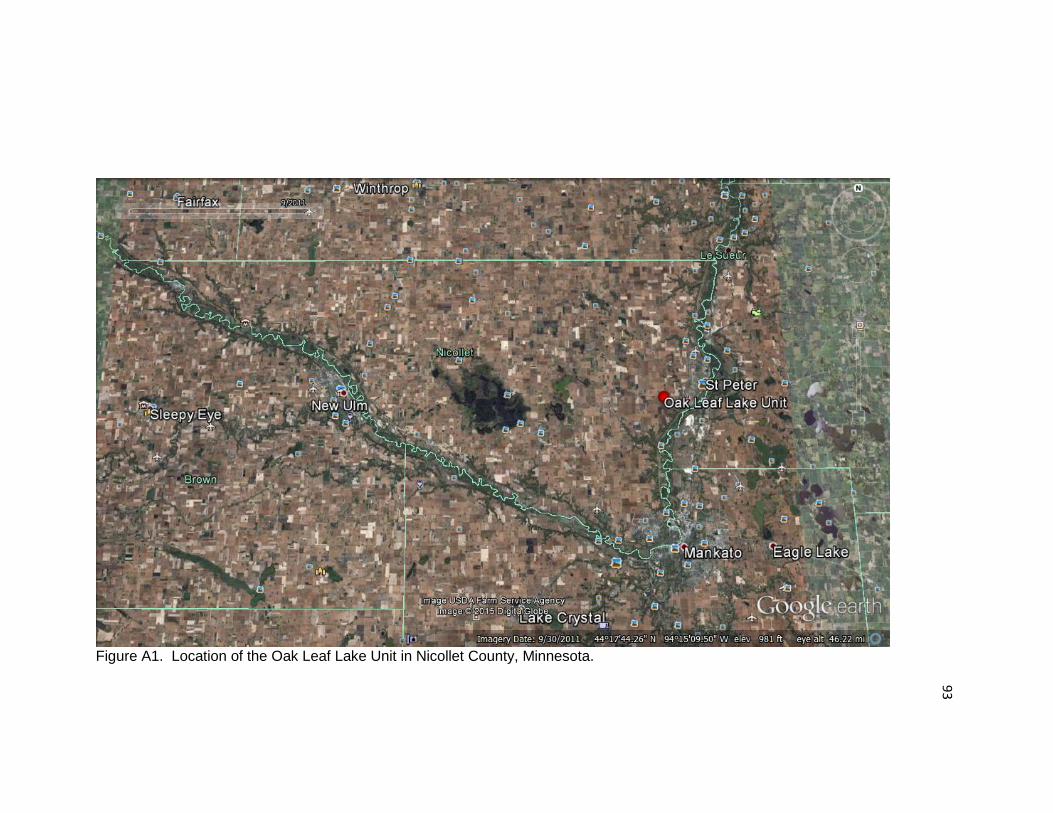
93

Figure A1. Location of the Oak Leaf Lake Unit in Nicollet County, Minnesota.

94

Figure A2. Map of the study site (within the white box) at the Oak Leaf Lake Unit and surrounding land.

95

Appendix B

Figure B1. Site map of the Oak Leaf Lake Unit showing study site divided into three

sections, dependent upon soil type, land formations and other habitat characteristics.

Section A is the most disturbed, with the driveway, parking area, and boat launch.

Section B is upland grassland area. Section C contains the two wetland areas within the

study site. Soil types are also shown. Soil type 109 is Cordova clay loam. Soil type

1075 is Klossner–Muskego soils, ponded. Soil type 978 is Cordova– Rolfe complex.

Soil type 239 is Le Sueur clay loam.

Figure B1. Site map of the Oak Leaf Lake Unit showing study site divided into three sections and by soil types.

96

Appendix C

Table C1. Soil types and descriptions found at the Oak Leaf Lake Unit as determined by

the USDA. Column 1 lists soil type. Column 2 describes the elevation. Column 3 lists

the mean annual precipitation and column 4 lists the mean annual air temperature. The

frost free period is located in Column 5. Column 6 describes landforms. Column 7 gives

slope percentage and Column 8 denotes drainage class. The capacity of the most limiting

layer to transmit water is listed in Column 9. Column 10 is the depth of the water table in

inches. Column 11 lists the frequency of flooding and Column 12 lists the frequency of

ponding. The maximum calcium carbonate content of each soil type is listed in Column

13. Column 14 lists the available water capacity.

97

Table C1. Soil types and descriptions found at the Oak Leaf Lake Unit.

Soil Type and Location at Site

Elevation (m)

Mean Annual

Precipitation (cm)

Mean Annual Air

Temperature (° C)

Frost-free

Period (Days) Landform

Slope (%)

Drainage Class

Capacity of Most

Limiting Layer to Transmit

Water

Depth Water Table (cm)

Frequency of

Flooding

Frequency of

Ponding

Calcium Carbonate Maximum Content

Available Water

Capacity

109 - Cordova clay loam

(western half from

driveway/parking lot to middle)

213 - 479 58 - 89 6 - 10 155 - 200

flats on moraines, swales on moraines

0 - 2 poorly

drained

moderately low to

moderately high

(0.36 - 1.45 cm/hr)

about 15 - 46

none none 0.2 high

(about 25 cm)

239 - Le Sueur clay loam (middle of

eastern side)

213 - 479 58 - 89 6 - 10 155 - 200

rises on moraines

1 - 3 somewhat

poorly drained

moderately high to

high (1.45 - 5.03

cm/hr)

about 46 - 76

none none 0.3 high

(about 27 cm)

978 - Cordova-Rolfe complex

(northwest portion and middle of

eastern half)

213 - 479 58 - 89 6 - 10 155 - 200

flats on moraines, swales on moraines

0 - 2 poorly

drained

moderately low to

moderately high

(0.36 - 1.45 cm/hr)

about 15 - 46

none none 0.2 high

(about 26 cm)

1075 - Klossner-Muskego soils,

ponded (shoreline)

213 - 479 58 - 89 6 - 10 155 - 200

depressions on

moraines 0 - 1

very poorly

drained

moderately low to high (0.36 - 5.03

cm/hr)

about 0

none frequent 0.2 very high

(about 50 cm)

98

Appendix D

Table D1. Plant species and collection data from the 2011-2012 Oak Leaf Lake Unit

survey. Nomenclature per Gleason and Cronquist (1991). Origin status indicates whether

the species is native (N), nonnative (NN), or unknown (U) (USDA 2012b). Section

indicates the area in which the species were located on the site (Figure B1). 2011 Coll

Date indicates the date when the voucher specimen was collected. Relocated in 2012

indicates whether the species was relocated using the random-sampling method.

Bloom/Fruit Season indicates the time period in which species observed in 2011 were in

bloom or fruit (I = June 3 – July 6, II = July 7 – August 13, and III = August 14 –

September 23). All vouchers are housed at the Radichel Herbarium at Minnesota State

University, Mankato.

99

Table D1. Plant survey data from the 2011-2012 Oak Leaf Lake Unit.

Fa

mil

y

Sp

ec

ies

Co

mm

on

Na

me

Ori

gin

Sta

tus

Co

lle

cti

on

#

Se

cti

on

20

11

Co

ll

Da

te

Re

loc

ate

d

in 2

012

Blo

om

/Fru

it

Se

as

on

Aceraceae (Maple)

Acer saccharum

Marshall sugar maple N 116 A 9/23 X III

Alismataceae (Water Plantain)

Sagittaria sp. arrowhead N 115 A 9/5 III

Apiaceae (Carrot)

Cicuta maculata L. common water hemlock

N 42 C 7/1 X I

Apiaceae (Carrot)

Pastinaca sativa L.

wild parsnip NN 33 ABC 6/26 X I

Apiaceae (Carrot)

Zizia aurea (L.)

Koch common golden alexander

N 4 ABC 6/13 X I

Asclepiadaceae (Milkweed)

Asclepias incarnata L.

swamp milkweed N 61 A 7/21 II


Asclepias syriaca

L. common milkweed N 96 B 8/25 X III


Asclepias tuberosa L.

butterfly-weed N 55 A 7/7 II

Asteraceae (Sunflower)

Achillea millefolium L.

common yarrow N 27 C 6/26 I


Ambrosia artemisiifolia L.

common ragweed N 76 A 7/31 X II


Ambrosia trifida L. giant ragweed N 86 A 8/6 X II


Anthemis cotula L. dogfennel, stinking chamomile

NN 58 A 7/13 X II


Arctium minus Schk.

common burdock NN 62 A 7/21 X II


Aster oolentangiense Riddell

prairie heart-leaved aster

N 124 AB 9/23 III


Aster sagittifolius

Wiild arrow-leaved aster N 123 A 9/23 III


Aster sp. aster U 113 ABC 9/5 X III


Aster sp. aster U 102 C 8/25 X III


Cirsium arvense Wimmer & Graebner var. horridum

Canada thistle NN 38 ABC 7/1 X I


Cirsium vulgare (Savi) Tenore

bull thistle NN 92 A 8/14 X III


Conyza canadensis (L.) Cronq.

horseweed N 75 A 7/31 II

100

Fa

mil

y

Sp

ec

ies

Co

mm

on

Na

me

Ori

gin

Sta

tus

Co

lle

cti

on

#

Se

cti

on

20

11

Co

ll

Da

te

Re

loc

ate

d

in 2

012

Blo

om

/Fru

it

Se

as

on


Erigeron strigosus Muhl var. strigosus

rough fleabane N 2 ABC 6/13 I


Euthamia gymnospermoides Greene

Great Plains flat-topped goldenrod

N 78 B 7/31 II


Helenium autumnale L.

common sneezeweed

N 68 ABC 7/31 X II


Helianthus grosseserratus Martens

sawtooth sunflower N 73 ABC 7/31 X II


Helianthus maximilianii Schrader

Maximillian sunflower

N 98 ABC 8/25 X III


Heliopsis helianthoides L.

common oxeye, smooth oxeye, false sunflower

N 29 ABC 6/26 I


Lactuca canadensis L.

tall lettuce N 101 ABC 8/25 X III


Liatris pycnostachya Michx.

prairie blazing star N 87 B 8/6 II


Ratibida pinnata (Vent.) Barnhart

prairie, grey-headed, or globular coneflower

N 57 ABC 7/13 X II


Rudbeckia hirta Farw var. pulcherrima

black-eyed Susan N 39 ABC 7/1 X I


Solidago canadensis L. var. canadensis

Canada goldenrod, common goldenrod

N 99 ABC 8/25 X III


Solidago canadensis Rydb.

var. gilvocanescens

Canada goldenrod, common goldenrod

N 112 ABC 9/5 III


Solidago missouriensis

Nutt. Missouri goldenrod N 100 ABC 8/25 III


Solidago nemoralis Aiton.

gray goldenrod N 111 B 9/5 X III


Solidago rigida L. stiff goldenrod N 110 B 9/5 X III


Sonchus arvensis L.

perennial sow-thistle

NN 47 ABC 7/7 X II


Taraxacum officinale Weber ex. Wiggers

common dandelion NN 11 A 6/19 X I

101

Fa

mil

y

Sp

ec

ies

Co

mm

on

Na

me

Ori

gin

Sta

tus

Co

lle

cti

on

#

Se

cti

on

20

11

Co

ll

Da

te

Re

loc

ate

d

in 2

012

Blo

om

/Fru

it

Se

as

on


Tragopogon dubius Scop

fistulous goat's beard

NN 49 BC 7/7 II


Vernonia fasciculata Michx. var. fasciculata

smooth ironweed N 90 A 8/6 II

Balsaminaceae (Touch-Me-Not)

Impatiens capensis Meerb.

orange forget-me-not, orange jewelweed

N 88 A 8/6 II

Brassicaceae (Mustard)

Hesperis matronalis L.

Dame's rocket, sweet rocket

NN 7 A 6/13 I

Brassicaceae (Mustard)

Thlaspi arvense L. field pennycress NN 6 A 6/13 X I

Caprifoliaceae (Honeysuckle)

Lonicera sp. honeysuckle U 59 B 7/13 II

Caprifoliaceae (Honeysuckle)

Sambucus canadensis L.

common elder, American elderberry

N 84 ABC 8/6 X II

Caryophyllaceae (Pink)

Silene latifolia Poiret

white campion, white cockle

NN 50 BC 7/7 II

Convolvulaceae (Morning Glory)

Calystegia sepium

(L.) R. Br. hedge bindweed NN 54 A 7/7 II

Cupressaceae (Cypress)

Juniperus virginiana L.

Eastern red cedar N 122 A 9/23 X III

Cyperaceae (Sedge)

Carex bebbii (L.H.

Bailey) Fern Bebb's sedge N 48 BC 7/7 II

Cyperaceae (Sedge)

Carex rostrata Stokes

beaked sedge N 31 BC 6/26 X I

Cyperaceae (Sedge)

Carex vulpinoidea

Michx var. vulpinoidea

fox sedge N 15 BC 6/19 I

Cyperaceae (Sedge)

Cyperaceae sp. sedge U 95 C 8/14 III

Cyperaceae (Sedge)

Cyperus esculentus L.

yellow nutsedge NN 91 A 8/6 II

Cyperaceae (Sedge)

Cyperus strigosus L.

false nutsedge N 93 C 8/14 III

Cyperaceae (Sedge)

Eleocharis palustris L.

common spikerush, creeping spike-rush

N 36 C 7/1 I

Cyperaceae (Sedge)

Scirpus maritimus L. (A. Nels.) Kuk var. paludosus

prairie bulrush, alkali bulrush

N 21 C 6/19 X I

Cyperaceae (Sedge)

Scirpus validus Vahl

softstem bulrush, great bulrush, common bulrush

N 34 C 6/26 X I

Fabaceae (Legume)

Amorpha canescens Pursh.

leadplant N 97 C 8/25 III

102

Fa

mil

y

Sp

ec

ies

Co

mm

on

Na

me

Ori

gin

Sta

tus

Co

lle

cti

on

#

Se

cti

on

20

11

Co

ll

Da

te

Re

loc

ate

d

in 2

012

Blo

om

/Fru

it

Se

as

on

Fabaceae (Legume)

Desmodium canadense L. (DC)

Canadian tick-trefoil

N 53 A 7/7 II

Fabaceae (Legume)

Medicago lupulina

L. black medick NN 46 A 7/1 I

Fabaceae (Legume)

Melilotus alba Medikus

white sweet clover NN 40 BC 7/1 I

Fabaceae (Legume)

Melilotus officinalis (L.) Pallas

yellow sweet clover NN 51 BC 7/7 II

Fabaceae (Legume)

Trifolium hybridum L.

alsike clover NN 3 AB 6/13 I

Fabaceae (Legume)

Trifolium pratense L.

red clover NN 70 A 7/31 X II

Fabaceae (Legume)

Trifolium repens L. white clover NN 44 A 7/1 I

Fabaceae (Legume)

Vicia americana Muhl var. americana

American vetch, wild vetch

N 5 C 6/13 X I

Fabaceae (Legume)

Vicia cracca L. bird vetch N 26 C 6/26 I

Iridaceae (Iris)

Iris virginica L. (Small) E. Anderson var. shrevei

southern blue flag iris

N 8 A 6/13 I

Lamiaceae (Mint) Agastache nepetoides (L.) Kuntze

catnip, giant hyssop

N 80 B 8/6 II

Lamiaceae (Mint) Lamiaceae sp. mint N 79 B 7/31 II

Lamiaceae (Mint) Leonurus cardiaca L.

motherwort NN 10 A 6/19 I

Lamiaceae (Mint) Monarda fistulosa L.

wild bergamot N 52 ABC 7/7 X II

Liliaceae (Lily) Allium stellatum

Ker Gawler. prairie onion N 89 C 8/6 II

Moraceae (Mulberry)

Morus alba L. white mulberry NN 118 A 9/23 X III

Nymphaeaceae (Water-Lily)

Nymphaea odorata Aiton

water lily N 69 A 7/31 II

Oleaceae (Olive) Fraxinus pennsylvanica Marshall

green ash N 119 ABC 9/23 X III

Oxalidaceae (Wood Sorrel)

Oxalis stricta L. common yellow wood-sorrel

N 45 A 7/1 X I

Plantaginaceae (Plantain)

Plantago major L. common plantain NN 43 A 7/1 X I

103

Fa

mil

y

Sp

ec

ies

Co

mm

on

Na

me

Ori

gin

Sta

tus

Co

lle

cti

on

#

Se

cti

on

20

11

Co

ll

Da

te

Re

loc

ate

d

in 2

012

Blo

om

/Fru

it

Se

as

on

Poaceae (Grass) Andropogon gerardii Vitman

big bluestem N 64 ABC 7/21 X II

Poaceae (Grass) Bromus commutatus

Schrader hairy chess brome NN 19 AB 6/19 X I

Poaceae (Grass) Bromus inermis Leysser

smooth brome NN 18 ABC 6/19 X I

Poaceae (Grass) Elytrigia repens L. quackgrass NN 28 BC 6/26 I

Poaceae (Grass) Panicum virgatum

L. switchgrass N 106 ABC 9/5 X III

Poaceae (Grass) Phalaris arundinacea L.

reed canary grass NN 14 ABC 6/19 X I

Poaceae (Grass) Phleum pratense

L. timothy NN 16 AB 6/19 I

Poaceae (Grass) Poa compressa L. Canada bluegrass NN 12 AB 6/19 I

Poaceae (Grass) Poa pratensis L. Kentucky bluegrass NN 109 ABC 9/5 X III

Poaceae (Grass) Poaceae sp. grass U 37 B 7/1 I

Poaceae (Grass) Setaria glauca (L.) P. Beauv.

yellow foxtail NN 85 A 8/6 II

Poaceae (Grass) Sorghastrum nutans (L.) Nash

Indian grass N 107 ABC 9/5 X III

Poaceae (Grass) Spartina pectinata Link.

prairie cord-grass N 83 C 8/6 X II

Poaceae (Grass)

Sphenopholis obtusata (Torr) K.S. Erdman var. major

wedge grass N 13 ABC 6/19 X I

Polygonaceae (Smartweed)

Polygonum amphibium (L.) Michx. var. emersum

water smartweed N 71 C 7/31 X II

Polygonaceae (Smartweed)

Rumex crispus L. curly dock NN 9 A 6/19 X I

Ranunculaceae (Buttercup)

Thalictrum dasycarpum Fischer & Ave-Lall.

purple meadow rue, tall meadow rue

N 23 C 6/26 I

Rosaceae (Rose) Geum canadense Jacq.

white avens N 32 A 6/26 I

Rosaceae (Rose) Pyrus malus L. crab apple NN 120 A 9/23 III

Rosaceae (Rose) Rosa carolina L. Carolina rose N 24 C 6/26 X I

Rubiaceae (Madder)

Galium boreale L. northern bedstraw N 1 B 6/13 I

104

Fa

mil

y

Sp

ec

ies

Co

mm

on

Na

me

Ori

gin

Sta

tus

Co

lle

cti

on

#

Se

cti

on

20

11

Co

ll

Da

te

Re

loc

ate

d

in 2

012

Blo

om

/Fru

it

Se

as

on

Salicaceae (Willow)

Populus alba L. white poplar NN 117 A 9/23 X III

Salicaceae (Willow)

Salix exigua Nutt. sandbar willow N 104 B 8/25 X III

Scrophulariaceae (Figwort)

Verbascum thapsus L.

common mullein NN 60 A 7/13 II


Veronica longifolia L.

long-leaved speedwell

N 63 A 7/21 II


Veronicastrum virginicum (L.) Farw.

Culver's root N 67 B 7/31 II

Solanaceae (Nightshade)

Physalis heterophylla Nees.

clammy ground cherry

N 105 A 9/5 X III

Solanaceae (Nightshade)

Solanum dulcamara L.

bittersweet nightshade

NN 25 C 6/26 I

Typhaceae (Cattail)

Typha angustifolia L.

narrow-leaved cattail

NN 35 ABC 6/26 X I

Ulmaceae (Elm) Ulmus sp. elm U 121 A 9/23 X III

Urticaceae (Nettle)

Urtica dioica L. stinging nettle N 114 A 9/5 X III

Verbenaceae (Vervain)

Verbena hastata L.

common or blue vervain

N 66 A 7/31 X II


Verbena stricta Vent.

hoary vervain N 94 A 8/14 III


Verbena urticifolia L.

white vervain N 74 A 7/31 II

Vitaceae (Grape) Vitis riparia Michx. frost grape, river-bank grape

N 82 AB 8/6 X II

105

Appendix E

The table included in Appendix E provides information for each species located at

the study site, including duration and wetland code. Duration is the length of the species'

life. Annuals perform their entire life cycle in one growing season. Biennials have a

two-year cycle, with root, stems, and leaves produced in the first growing season and

reproductive parts (flowers, fruit, and seeds) produced in the second growing season.

Perennials live three or more years.

Wetland codes are assigned to species to determine their presence as an indicator

of a wetland. Obligate wetland species almost always occur in wetlands. Facultative

wetland species usually occur in wetlands, but may also occur in non-wetlands.

Facultative species can occur either in wetlands or not. Facultative upland species

usually occur in non-wetlands, but can be found in wetlands. Obligate upland species

almost never occur in wetlands.

Table E1. Life history data, ecological requirements and indicator/weed status for plant

species at the Oak Leaf Lake Unit. Nomenclature per Gleason and Cronquist (1991).

Growth habits are indicated as follows: forb (F), grass (G), shrub (S), subshrub (SS), tree

(T), and vine (V). Duration indicates if species are annual (A), biennial (B), or perennial

(P). The habitat each species is most likely to be found in includes disturbed areas (DA),

ditches (D), fields (F), lawns (L), marshes (Ma), meadow (Me), open places (OP),

prairies (P), roadsides (R), shorelines (Sh), streambanks (St), swamps (Sw), thickets (T),

waste places (WP), and woods (W). Wetland code are assigned as obligate wetland

(OBL), facultative wetland (FACW), facultative (FAC), facultative upland (FACU), and

obligate upland (UPL) (Ladd 2005; Lichvar et al. 2014). C-values range from 0-10 for

native species, an asterisk indicates nonnative species, and none (N) indicates species are

not listed (TNGPFQAP 2001; Ladd 2005). Indicator species are listed as Tier 1 (1) or

Tier 2 (2) by the Minnesota County Biological Survey (Carlson 2010; MN DNR 2012a)

or (C) if listed by Curtis (1955; 1971). Invasive species listed by the Minnesota County

Biological Survey (Carlson 2010; MN DNR 2012a) Tier 1 (1) and Tier 2 (2). Weed

status: MDA MN Prohibited Noxious Weeds (P) (2010, 2012), MDA MN Secondary

Noxious Weeds (S) (2010, 2012), and “undesirable species” listed by Gleason and

Cronquist (G) (1991) and University of Minnesota Extension (U) (2015a, 2015b, 2015c).

106

Table E1. Life history data, ecological requirements and indicator/weed status for plant species at the Oak Leaf Lake Unit.

Sp

ec

ies

Gro

wth

Ha

bit

Du

rati

on

Blo

om

Pe

rio

d/

Fru

itin

g

Se

as

on

Ha

bit

at

We

tla

nd

Co

de

C-v

alu

e

Ind

ica

tor

Sp

ec

ies

Inv

as

ive

Sp

ec

ies

We

ed

Sta

tus

Ea

rly

-

Su

cc

ess

ion

al

At

Ka

so

ta

Pra

irie

Acer saccharum Marshall

S, T P Ap, M Jun W FACU 10

Achillea millefolium L. F P Jun, Jul, Au, S, O

DA, F, R, WP

FACU 3

X

Agastache nepetoides (L.) Kuntze

F, SS

P Au, S W FACU 8

Allium stellatum Ker Gawler.

F P Jul, Au, S P UPL 7

X

Ambrosia artemisiifolia L.

F A Jul, Au, S, O

WP FACU 0

G, U, S

X X

Ambrosia trifida L. F, SS

A Jul, Au, S, O

WP FAC 0

G, U, S

X X

Amorpha canescens Pursh.

S, SS

P Jun, Jul P, W UPL 9 1

X

Andropogon gerardii Vitman

G P Jul, Au OP FAC 5

X

Anthemis cotula L. F A Jun, Jul, Au, S

F, WP FACU *

G X

Arctium minus Schk. F B Jul, Au, S R, WP

FACU *

2 U, S X

Asclepias incarnata L. F P Jun, Jul, Au

D, P, Sw

OBL 5

Asclepias syriaca L. F P Jun, Jul, Au

F, Me, R

FACU 0

S

X

Asclepias tuberosa L. F P Jun, Jul, Au

P, W UPL 9 2

X

Aster oolentangiense Riddell

F, SS

P Au, S, O P, W UPL 10 2

Aster sagittifolius

Wiild F P

Jul, Au, S, O

OP, St, W

NL 8

Aster sp. P P Unknown U U N

Aster sp. P P Unknown U U N

Bromus commutatus Schrader

G A M, Jun, Jul

DA NL N

X

Bromus inermis Leysser

G P Jun, Jul

DA, D, F, OP, P, R

FACU *

1

X

Calystegia sepium

(L.) R. Br. F, V P

Jun, Jul, Au

DA, Sh, T

FAC 0

2

X

107

Sp

ec

ies

Gro

wth

Ha

bit

Du

rati

on

Blo

om

Pe

rio

d/

Fru

itin

g

Se

as

on

Ha

bit

at

We

tla

nd

Co

de

C-v

alu

e

Ind

ica

tor

Sp

ec

ies

Inv

as

ive

Sp

ec

ies

We

ed

Sta

tus

Ea

rly

-

Su

cc

ess

ion

al

At

Ka

so

ta

Pra

irie

Carex bebbii (L.H. Bailey) Fern

G P Jun, Jul Me, Sh

OBL 8

Carex rostrata Stokes G P Jun, Jul, Au

Sh OBL 8

Carex vulpinoidea Michx var. vulpinoidea

G P M, Jun Ma, Sh, Sw

FACW 2

Cicuta maculata L. F P Jun, Jul, Au

D, Ma, Sw

OBL 4 C

Cirsium arvense Wimmer & Graebner var. horridum

F P Jul, Au F, WP FACU *

1 G,

U, P X

Cirsium vulgare

(Savi) Tenore F B

Jun, Jul, Au, S, O

F, R, P, WP

FACU *

1 G,

U, P

Conyza canadensis (L.) Cronq.

F A Jul, Au, S, O

F, WP NL 0

G X X

Cyperaceae sp. G P Unknown U U N

Cyperus esculentus L.

G P Jul, Au, S Ma, Sh, Sw

FACW 0

G, U, S

Cyperus strigosus L. G P Au, S, O F, Sh, Sw

FACW 3

Desmodium canadense L. (DC)

F P Jul, Au St, T FACU 6 C

Eleocharis palustris L. G P M, Jun, Jul, Au

Ma, Sh, Sw

OBL N

Elytrigia repens L. G P Jun, Jul DA NL N

1 G,

U, S

Erigeron strigosus Muhl var. strigosus

F A, B Jun, Jul, Au, S

DA FACU 3

G X X

Euthamia gymnospermoides Greene

F P Jul, Au, S OP FACW 5

Fraxinus pennsylvanica Marshall

T P M, Jun W FACW 5

Galium boreale L. F, SS

P Jun, Jul Me, St, W

FAC 4 C

X

Geum canadense Jacq.

F P M, Jun W FAC 4

Helenium autumnale

L. F P

Jul, Au, S, O

Sh, St FACW 4 1

108

Sp

ec

ies

Gro

wth

Ha

bit

Du

rati

on

Blo

om

Pe

rio

d/

Fru

itin

g

Se

as

on

Ha

bit

at

We

tla

nd

Co

de

C-v

alu

e

Ind

ica

tor

Sp

ec

ies

Inv

as

ive

Sp

ec

ies

We

ed

Sta

tus

Ea

rly

-

Su

cc

ess

ion

al

At

Ka

so

ta

Pra

irie

Helianthus grosseserratus

Martens F P Au, S, O

F, Me, P

FACW 7 C

X

Helianthus maximilianii Schrader

F P Jul, Au, S, O

P, WP

UPL 5

Heliopsis helianthoides L.

F P Jul, Au, S P, WP, W

FACU 5

X

Hesperis matronalis L.

F B, P M, Jun F, W FACU *

Impatiens capensis Meerb.

F A Jun, Jul, Au, S

D, St, W

FACW 4

X

Iris virginica L. (Small) E. Anderson var. shrevei

F P M, Jun, Jul

D, Ma, Me, S

OBL N

Juniperus virginiana L.

T P M, Jun, Jul

DA, Me, OP, P, W

FACU 0

X

Lactuca canadensis

L. F A, B Jul, Au, S

F, WP, W

FACU 6

X X

Lamiaceae sp. U U Unknown U U N

Leonurus cardiaca L. F P Jun, Jul, Au, S

DA, R, WP

NL *

G

X

Liatris pycnostachya Michx.

F P Jul, Au, S P, W FAC 8 1

Lonicera sp. S P Unknown U U N

Medicago lupulina L. F A, B M, Jun, Jul, Au, S

P, R FACU *

2 G, U X X

Melilotus alba Medikus

F A, B Jun, Jul, Au, S, O

R, WP

NL *

1 G X X

Melilotus officinalis (L.) Pallas

F A, B Jun, Jul, Au, S

WP FACU *

1 G X X

Monarda fistulosa L. F, SS

P Jun, Jul, Au, S

P, T, W

FACU 5

X

Morus alba L. S, T P M, Jun DA, F, R, W

FAC *

2

Nymphaea odorata Aiton

F P Jun, Jul, Au, S

Sh OBL 9

Oxalis stricta L. F P Jun, Jul, Au, S, O

F, R, WP

FACU 0

G, U

X

109

Sp

ec

ies

Gro

wth

Ha

bit

Du

rati

on

Blo

om

Pe

rio

d/

Fru

itin

g

Se

as

on

Ha

bit

at

We

tla

nd

Co

de

C-v

alu

e

Ind

ica

tor

Sp

ec

ies

Inv

as

ive

Sp

ec

ies

We

ed

Sta

tus

Ea

rly

-

Su

cc

ess

ion

al

At

Ka

so

ta

Pra

irie

Panicum virgatum L. G P Jun, Jul, Au

Ma, P, Sh, W

FAC 5

X

Pastinaca sativa L. F B Jun, Jul F, R, WP

NL *

1 G, U X

Phalaris arundinacea

L. G P Jun, Jul

Ma, Sh, St

FACW 0

1 U

X

Phleum pratense L. G P Jun, Jul, Au

DA, F, P

FACU *

1

X

Physalis heterophylla

Nees. F P

Jun, Jul, Au, S

P, W UPL 5

X

Plantago major L. F P Jun, Jul, Au, S, O

L, R, WP

FAC *

2 U X

Poa compressa L. G P Jun, Jul OP, R FACU *

1

X

Poa pratensis L. G P Jun, Jul

DA, D, L, P, R, WP

FAC *

1

X

Poaceae sp. G U Unknown U U N

Polygonum amphibium (L.) Michx. var. emersum

F P Jul, Au, S

Ma, Sh, St, Sw

OBL 0

Populus alba L. T P Ap, M DA, F, Me

NL *

Pyrus malus L. S, T P M, Jun DA, Me, R

NL N

Ratibida pinnata (Vent.) Barnhart

F P Jun, Jul, Au

F, P, W

UPL 6 C

Rosa carolina L. SS P M, Jun

DA, F, Me, OP, P, R

FAC N

Rudbeckia hirta Farw var. pulcherrima

F B, P Jun, Jul, Au, S, O

Me, P, R

FACU 5 C

X X

Rumex crispus L. F P Jun, Jul R, WG, F

FAC *

2 G, S X

Sagittaria sp. P P Unknown U U N

Salix exigua Nutt. S, T P Ap, M Ma, Sh, Sw

OBL 3

110

Sp

ec

ies

Gro

wth

Ha

bit

Du

rati

on

Blo

om

Pe

rio

d/

Fru

itin

g

Se

as

on

Ha

bit

at

We

tla

nd

Co

de

C-v

alu

e

Ind

ica

tor

Sp

ec

ies

Inv

as

ive

Sp

ec

ies

We

ed

Sta

tus

Ea

rly

-

Su

cc

ess

ion

al

At

Ka

so

ta

Pra

irie

Sambucus canadensis L.

S, T P Jul, Au F, R, W

FACU 4

Scirpus maritimus L. (A. Nels.) Kuk var. paludosus

G P Jun, Jul, Au, S

Ma, Sh, Sw

NL 4

Scirpus validus Vahl G P Jun, Jul, Au

Ma, Sh, Sw

OBL 3

Setaria glauca (L.) P. Beauv.

G P M, Jun, Jul, Au, S

DA, F, WP

FAC *

2 G, U

Silene latifolia Poiret F A, B, P

M, Jun, Jul, Au, S

F, R, WP

NL N

G X

Solanum dulcamara L.

F, SS, V

P Jun, Jul, Au, S

OP, T, W

FAC *

Solidago canadensis L. var. canadensis

F P Jul, Au, S, O

OP, W

FACU 1

X

Solidago canadensis Rydb. var. gilvocanescens

F P Jul, Au, S, O

OP, W

FACU 1

X

Solidago missouriensis Nutt.

F P Jul, Au, S OP, P, W

UPL 5 C

X

Solidago nemoralis Aiton.

F P Au, S, O OP, W

UPL 6 C

X

Solidago rigida L. F P Au, S, O OP, P FACU 4

X

Sonchus arvensis L. F P Jul, Au, S, O

DA, F, R

FACU *

1 G,

U, P

Sorghastrum nutans (L.) Nash

G P Au, S F, P, W

FACU 6 2

X

Spartina pectinata Link.

G P Jun, Jul Ma, Sh

FACW 5 C

X

Sphenopholis obtusata (Torr) K.S. Erdman var. major

G P M, Jun Me, Sh, St

FAC 7

Taraxacum officinale

Weber ex. Wiggers F P

Ap, M, Jun, Jul, Au, S, O

DA, L FACU *

2 G, U X X

Thalictrum dasycarpum Fischer & Ave-Lall.

F P Jun, Jul Me, Sh, St

FACW 7 2, C

X

Thlaspi arvense L. F A Ap, M, Jun WP FACU *

X

Tragopogon dubius Scop

F B M, Jun, Jul

OP, R NL *

X X

111

Sp

ec

ies

Gro

wth

Ha

bit

Du

rati

on

Blo

om

Pe

rio

d/

Fru

itin

g

Se

as

on

Ha

bit

at

We

tla

nd

Co

de

C-v

alu

e

Ind

ica

tor

Sp

ec

ies

Inv

as

ive

Sp

ec

ies

We

ed

Sta

tus

Ea

rly

-

Su

cc

ess

ion

al

At

Ka

so

ta

Pra

irie

Trifolium hybridum L. F P Jun, Jul, Au, S

Me, P, R

FACU *

1

X

Trifolium pratense L. F P M, Jun, Jul, Au

F, R FACU *

1

X X

Trifolium repens L. F P Jun, Jul, Au, S

L, R FACU *

1 U

X

Typha angustifolia L. F P M, Jun Ma OBL *

Ulmus sp. T P Unknown U U N

X

Urtica dioica L. F P Jun, Jul, Au, S

DA, W

FACW 0

U

Verbascum thapsus L.

F B Jun, Jul, Au, S

DA UPL *

2

X X

Verbena hastata L. F P Jun, Jul, Au, S, O

F, Me, P, Sw

FACW 5

X

Verbena stricta Vent. F P Jun, Jul, Au, S

F, OP, P, R

UPL 2

X

Verbena urticifolia L. F P Jun, Jul, Au, S, O

F, Me, T, WP

FAC 3

Vernonia fasciculata Michx. var. fasciculata

F P Jul, Au, S P, Ma FACW 3

X

Veronica longifolia L. F P Jun, Jul,

Au F, R, WP

NL *

Veronicastrum virginicum (L.) Farw.

F P Jun, Jul,

Au P, W FAC 10

2, C

X

Vicia americana Muhl var. americana

F, V P M, Jun,

Jul W FACU 3

X

Vicia cracca L. F, V P Jun, Jul,

Au F,

Me, R NL N

Vitis riparia Michx. V P M, Jun R, T,

W FACW 3

U

X

Zizia aurea (L.) Koch F P M, Jun F, Me FAC 8 1, C

112

Appendix F

Figure F1-F3. Species area curves for “early-” (I = June 3 – July 6), “mid-” (II = July 7

– August 13), and “late-blooming/fruiting” (III = August 14 – September 23) periods of

the random sampling method.

Figure F1. Species area curve for Period I (the early-blooming/fruiting period) of the random-sampling method.

0

1

2

3

4

5

6

7

0 5 10 15 20 25 30 35 40 45 50 55 60 65 70 75 80

Me

an P

lan

t Sp

eci

es

Ric

hn

ess

Area (m2)

113

Figure F2. Species area curve for Period II (the mid-blooming/fruiting period) of the random-sampling method.

Figure F3. Species area curve for Period III (the late-blooming/fruiting period) of the random-sampling method.

0

1

2

3

4

5

6

7

0 5 10 15 20 25 30 35 40 45 50 55 60 65 70 75 80

Me

an P

lan

t Sp

eci

es

Ric

hn

ess

Area (m2)

0

1

2

3

4

5

6

7

0 5 10 15 20 25 30 35 40 45 50 55 60 65 70 75 80

Me

an P

lan

t Sp

eci

es

Ric

hn

ess

Area (m2)

114

Appendix G Table G1. Selected early-successional, nonnative, invasive, noxious (P = State Prohibited Noxious, S = State Secondary Noxious), and high-quality indicator (T-1 = Tier 1, T-2 = Tier 2, C = sensu Curtis [1955; 1971]) species found at the Oak Leaf Lake Unit, the section(s) within which they were located and their wetland codes, if known (OBL = obligate wetland, FACW = facultative wetland, FAC = facultative, FACU = facultative upland, and UPL = obligate upland [Ladd 2005; Lichvar et al. 2014]).

Sp

ecie

s

Earl

y-

su

cce

ssio

nal

Secti

on

(s)

Wetl

an

d c

od

e

No

nn

ati

ve

Invasiv

e

No

xio

us

Hig

h-q

uality

ind

icato

r

alexander, common golden

A B C FAC

T-1, C

aster, prairie-heart-leaved

A B UPL

T-2

bedstraw, northern

B FAC

C

black-eyed Susan x A B C FACU

C

blazing star, prairie

B FAC

T-1

burdock, common x A FACU x x S

campion, white x B C

x

clover, alsike x A B FACU x x

clover, red x A FACU x x

clover, white A FACU x x

clover, sweet white x B C

x x

clover, sweet yellow x B C FACU x x

coneflower, prairie

A B C UPL

C

Culver's root

B FAC

T-2, C

dandelion, common x A FACU x x

dock, curly x A FAC x x S

dogfennel x A FACU x

fleabane, rough x A B C FACU

goat's beard, fistulous x B C

x

goldenrod, gray

B UPL

C

goldenrod, Missouri

A B C UPL

C

grass, Canada blue-

A B FACU x x

grass, hairy chess x A B

x

grass, Indian

A B C FACU

T-2

grass, Kentucky blue-

A B C FAC x x

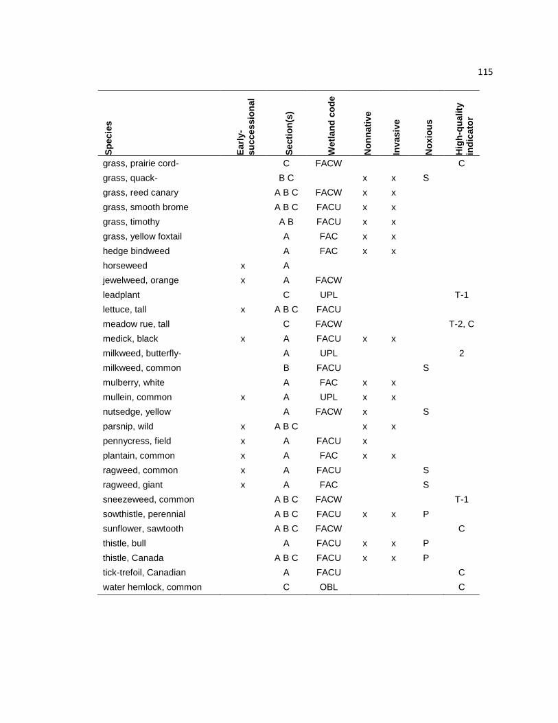
115

Sp

ecie

s

Earl

y-

su

cce

ssio

nal

Secti

on

(s)

Wetl

an

d c

od

e

No

nn

ati

ve

Invasiv

e

No

xio

us

Hig

h-q

uality

ind

icato

r

grass, prairie cord-

C FACW

C

grass, quack-

B C

x x S

grass, reed canary

A B C FACW x x

grass, smooth brome

A B C FACU x x

grass, timothy

A B FACU x x

grass, yellow foxtail

A FAC x x

hedge bindweed

A FAC x x

horseweed x A

jewelweed, orange x A FACW

leadplant

C UPL

T-1

lettuce, tall x A B C FACU

meadow rue, tall

C FACW

T-2, C

medick, black x A FACU x x

milkweed, butterfly-

A UPL

2

milkweed, common

B FACU

S

mulberry, white

A FAC x x

mullein, common x A UPL x x

nutsedge, yellow

A FACW x

S

parsnip, wild x A B C

x x

pennycress, field x A FACU x

plantain, common x A FAC x x

ragweed, common x A FACU

S

ragweed, giant x A FAC

S

sneezeweed, common

A B C FACW

T-1

sowthistle, perennial

A B C FACU x x P

sunflower, sawtooth

A B C FACW

C

thistle, bull

A FACU x x P

thistle, Canada

A B C FACU x x P

tick-trefoil, Canadian

A FACU

C

water hemlock, common

C OBL

C

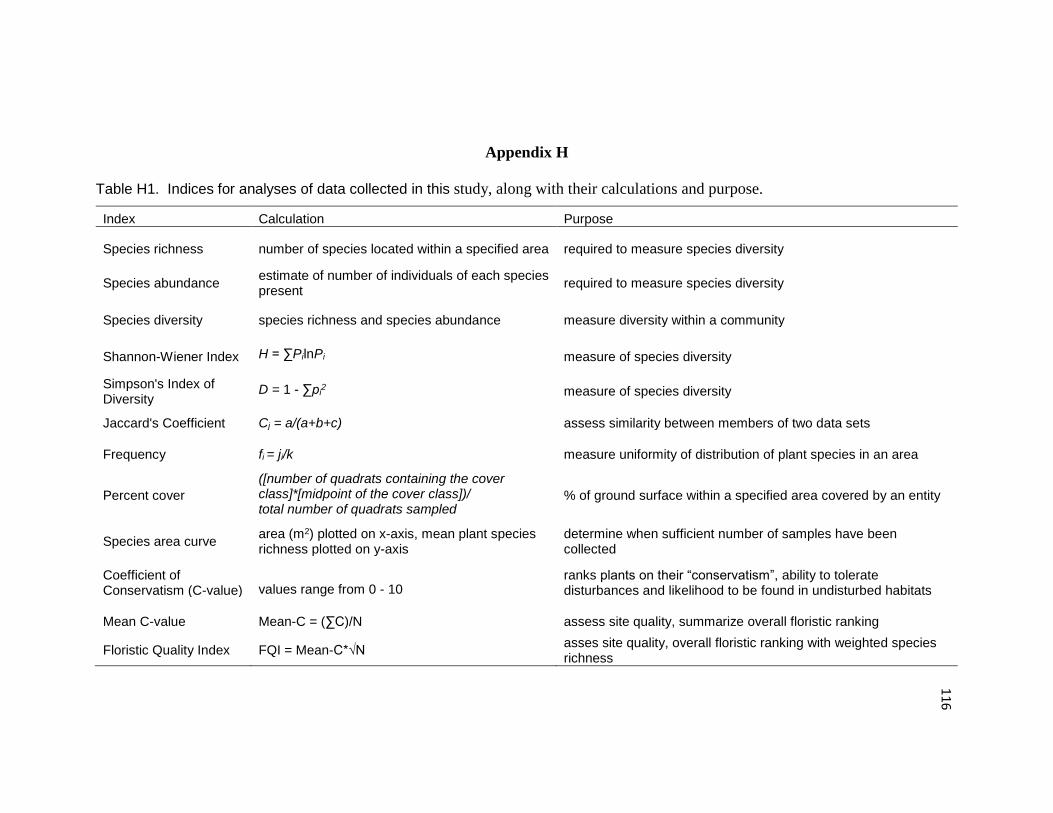
116

Appendix H

Table H1. Indices for analyses of data collected in this study, along with their calculations and purpose.

Index Calculation Purpose

Species richness number of species located within a specified area required to measure species diversity

Species abundance estimate of number of individuals of each species present

required to measure species diversity

Species diversity species richness and species abundance measure diversity within a community

Shannon-Wiener Index H = ∑PilnPi measure of species diversity

Simpson's Index of Diversity

D = 1 - ∑pi2 measure of species diversity

Jaccard's Coefficient Cj = a/(a+b+c) assess similarity between members of two data sets

Frequency fi = ji/k measure uniformity of distribution of plant species in an area

Percent cover

([number of quadrats containing the cover class]*[midpoint of the cover class])/ total number of quadrats sampled

% of ground surface within a specified area covered by an entity

Species area curve area (m2) plotted on x-axis, mean plant species richness plotted on y-axis

determine when sufficient number of samples have been collected

Coefficient of Conservatism (C-value) values range from 0 - 10

ranks plants on their “conservatism”, ability to tolerate disturbances and likelihood to be found in undisturbed habitats

Mean C-value Mean-C = (∑C)/N assess site quality, summarize overall floristic ranking

Floristic Quality Index FQI = Mean-C*√N asses site quality, overall floristic ranking with weighted species richness

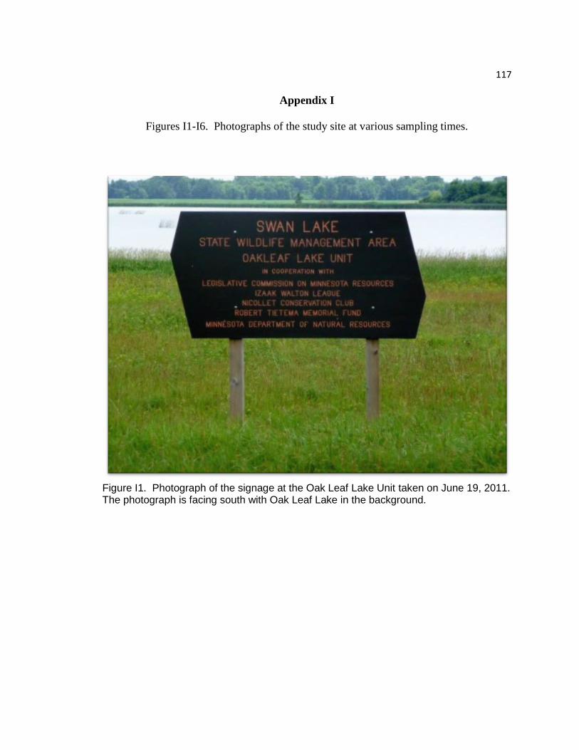
117

Appendix I

Figures I1-I6. Photographs of the study site at various sampling times.

Figure I1. Photograph of the signage at the Oak Leaf Lake Unit taken on June 19, 2011. The photograph is facing south with Oak Leaf Lake in the background.

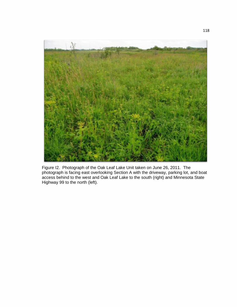
118

Figure I2. Photograph of the Oak Leaf Lake Unit taken on June 26, 2011. The photograph is facing east overlooking Section A with the driveway, parking lot, and boat access behind to the west and Oak Leaf Lake to the south (right) and Minnesota State Highway 99 to the north (left).

119

Figure I3. Photograph of the Oak Leaf Lake Unit taken on August 6, 2011. The photograph is facing southeast overlooking Sections A and B and Oak Leaf Lake.

120

Figure I4. Photograph of the Oak Leaf Lake Unit taken on August 6, 2011. The photograph is facing east overlooking Sections A and B and Oak Leaf Lake.

121

Figure I5. Photograph of the Oak Leaf Lake Unit taken on August 14, 2011. The photograph is facing east overlooking Section B with Oak Leaf Lake to the south (right) and Minnesota State Highway 99 to the north (left).

122

Figure I6. Photograph of the Oak Leaf Lake Unit taken on September 23, 2011. The photograph is facing east overlooking Section A with the driveway, parking lot, and boat access behind to the west and Oak Leaf Lake to the south (right) and Minnesota State Highway 99 to the north (left).

Documents

A Floristic Study of the Oak Leaf Lake Unit of the Swan