Embed Size (px)
Citation preview

A FLOQUET OPERATOR WITH PURE POINTSPECTRUM AND ENERGY INSTABILITY
CESAR R. DE OLIVEIRA AND MARIZA S. SIMSEN
Abstract. An example of Floquet operator with purely point spectrumand energy instability is presented. In the unperturbed energy eigenbasisits eigenfunctions are exponentially localized.
1. Introduction
It is not immediate whether a self-adjoint operator H with purely pointspectrum implies absence of transport under the time evolution U(t) =e−iHt; in fact, it is currently known examples of Schrodinger operators withsuch kind of spectrum and transport. In case of tight-binding models onl2(IN) the transport is usually probed by the moments of order m > 0 of theposition operator Xek = kek, that is,
Xm =∑
k∈IN
km〈ek, ·〉ek,(1)
where ek(j) = δkj (Kronecker delta) is the canonical basis of l2(IN). Analo-gous definition applies for l2(ZZ) and even higher dimensional spaces. Then,by definition, transport at ψ, also called dynamical instability or dynamicaldelocalization, occurs if for some m the function
t #→ 〈ψ(t), Xmψ(t)〉, ψ(t) := U(t)ψ,(2)
is unbounded. If for all m > 0 the corresponding functions are bounded,one has dynamical stability, also called dynamical localization.
The first rigorous example of a Schrodinger operator with purely pointspectrum and dynamical instability has appeared in [7], Appendix 2, whatthe authors have called “A Pathological Example;” in this case the tightbinding Schrodinger operator h on l2(IN) with a Dirichlet condition at n =−1 was
(hu)(n) = u(n + 1) + u(n − 1) + v(n)u(n)
with potential
v(n) = 3 cos(παn + θ) + λδn0,(3)
1991 Mathematics Subject Classification. 81Q10 (11B,47B99).CRdeO was partially supported by CNPq (Brazil).MSS was supported by CAPES (Brazil).
1
2 CESAR R. DE OLIVEIRA AND MARIZA S. SIMSEN
that is, rank one perturbations of an instance of the almost Mathieu opera-tor. An irrational number α was constructed so that for a.e. θ ∈ [0, 2π) anda.e. λ ∈ [0, 1] the corresponding self-adjoint operator h has purely point spec-trum with dynamical instability at e0 (throughout, the term “a.e.” withoutspecification means with respect to the Lebesgue measure under considera-tion). More precisely, it was shown that for all ε > 0
lim supt→∞
1t2−ε
〈ψ(t), X2ψ(t)〉 = ∞, ψ(0) = e0.
Compare with the absence of ballistic motion for point spectrum Hamilto-nians [16]
limt→∞
1t2〈ψ(t), X2ψ(t)〉 = 0.
Additional examples of this behavior are known, even for random po-tentials, but with a strong local correlations [10], as for the random dimermodel in the Schrodinger case; there is also an adaptation [6] for the randomBernoulli Dirac operator with no correlation in the potential, although forthe massless case.
The time evolution of a quantum system with time-dependent Hamilto-nian is given by a strongly continuous family of unitary operators U(t, r)(the propagator). For an initial condition ψ0 at t = 0, its time evolution isgiven by U(t, 0)ψ0. If the Hamiltonian is time-periodic with period T , then
U(t + T, r + T ) = U(t, r), ∀t, r,
and we have the Floquet operator UF := U(T, 0) defined as the evolutiongenerated by the Hamiltonian over a period.
Quantum systems governed by a time periodic Hamiltonian have theirdynamical stability often characterized in terms of the spectral properties ofthe corresponding Floquet operator. As in the autonomous case, the pres-ence of continuous spectrum is a signature of unstable quantum systems;this is a consequence of the famous RAGE theorem, firstly proved for theautonomous case [15] and then for time-periodic Hamiltonians [8]. In princi-ple, a Floquet operator with purely point spectrum would imply “stability,”but one should be alerted by the above mentioned “pathological” examplesin the autonomous case.
In this work we give an example of a Floquet operator with purely pointspectrum and “energy instability,” which can be considered the partnerconcept of dynamical instability in case of autonomous systems. We shallconsider a particular choice in the family of Floquet operators studied in [3];such operators describe the quantum dynamics of certain interesting physi-cal models (see [1, 3] and references therein), and display a band structurewith respect to an orthogonal basis ϕk of l2(IN) or l2(ZZ), constructed aseigenfunctions of an unperturbed energy operator. There are some concep-tual differences with respect to the autonomous case mentioned before, since

PURE POINT AND ENERGY INSTABILITY 3
now the momentum Xm is defined in the energy space
Xm =∑
k≥1
km〈ϕk, ·〉ϕk,(4)
instead of the “physical space” IN. Thus, if for all m > 0 the functions
n #→ 〈ψ(n), Xmψ(n)〉, ψ(n) := UnFψ, n ≥ 0,(5)
are bounded we say there is energy stability or energy localization, while if atleast one of them is unbounded we say the system presents energy instabilityor energy delocalization; the latter reflects a kind of “resonance.”
Our construction is a fusion of the Floquet operator studied in [3], nowunder suitable additional rank one perturbations, and the arguments pre-sented in [7] for model (3). For suitable values of parameters we shall getthe following properties:
1. The resulting unitary operator Uλ(β, θ)+ (after the rank one pertur-bation; see Eq. (10)) still belongs to the family of Floquet operatorsconsidered in [3].
2. Uλ(β, θ)+ has purely point spectrum with exponentially localized eigen-functions.
3. The time evolution along the Floquet operator Uλ(β, θ)+ of the initialcondition ϕ1 presents energy instability.
Uλ(β, θ)+ will be obtained as a rank one perturbation of the almost pe-riodic class of operators studied in the Section 7 of [3] (we describe themahead). In order to prove purely point spectrum, we borrow an argumentfrom [9] that was used to prove localization for random unitary operators,and it combines spectral averaging and positivity of the Lyapunov exponentwith polynomial boundedness of generalized eigenfunctions. In order to getdynamical instability, although we adapt ideas of [7], we underline that someresults needed completely different proofs and they are not entirely trivial.
It is worth mentioning that in [19] a form of dynamical stability was ob-tained for discrete evolution along some Floquet operators (CMV matrices)related to random Verblunsky coefficients.
This paper is organized as follows. In Section 2 we present the model ofFloquet operator we shall consider, some preliminary results and the mainresult is stated in Theorem 2. In Section 3 we shall prove that our Floquetoperator is pure point. Section 4 is devoted to the proof of dynamicalinstability.
2. The Floquet Operator
We briefly recall the construction of the Floquet operator introduced in [3]based on the physical model discussed in [1]. The separable Hilbert spaceis l2(ZZ) and ϕkk∈ZZ denote its canonical basis. Consider the set of 2 × 2

4 CESAR R. DE OLIVEIRA AND MARIZA S. SIMSEN
matrices defined for any k ∈ ZZ by
Sk = e−iθk
(re−iαk iteiγk
ite−iγk reiαk
)
parameterized by the phases αk, γk, θk in the torus T and the real pa-rameters t, r, the reflection and transition coefficients, respectively, linkedby r2 + t2 = 1. Then, let Pj be the orthogonal projection onto the spanof ϕj , ϕj+1 in l2(ZZ), and let Ue, Uo be two 2 × 2 block diagonal unitaryoperators on l2(ZZ) defined by
Ue =∑
k∈ZZ
P2kS2kP2k and Uo =∑
k∈ZZ
P2k+1S2k+1P2k+1.
The matrix representation of Ue in the canonical basis is
Ue =
. . .S−2
S0
S2. . .
,
and similarly for Uo, with S2k+1 in place of S2k. The Floquet operator U isdefined by
U = UoUe,
such that, for any k ∈ ZZ,
Uϕ2k = irte−i(θ2k+θ2k!1)e−i(α2k−γ2k!1)ϕ2k−1
+r2e−i(θ2k+θ2k!1)e−i(α2k−α2k!1)ϕ2k
+irte−i(θ2k+θ2k+1)e−i(γ2k+α2k+1)ϕ2k+1
−t2e−i(θ2k+θ2k+1)e−i(γ2k+γ2k+1)ϕ2k+2
Uϕ2k+1 = −t2e−i(θ2k+θ2k!1)ei(γ2k+γ2k!1)ϕ2k−1(6)+irte−i(θ2k+θ2k!1)ei(γ2k+α2k!1)ϕ2k
+r2e−i(θ2k+θ2k+1)ei(α2k−α2k+1)ϕ2k+1
+irte−i(θ2k+θ2k+1)ei(α2k−γ2k+1)ϕ2k+2
The extreme cases where rt = 0 are spectrally trivial; in case t = 0,r = 1, U is pure point and if t = 1, r = 0, U is purely absolutely continuous(Proposition 3.1 in [3]). From now on we suppose 0 < r, t < 1.
For the eigenvalue equation
Uψ = eiEψ
ψ =∑
k∈ZZ
ckϕk, ck, E ∈ C,

PURE POINT AND ENERGY INSTABILITY 5
one gets the following relation between coefficients(
c2k
c2k+1
)= Tk(E)
(c2k−2
c2k−1
),
where the matrix Tk(E) has elements
Tk(E)11 = −e−i(E+γ2k!1+γ2k!2+θ2k!1+θ2k!2),
Tk(E)12 = ir
t
(e−i(E+γ2k!1−α2k!2+θ2k!1+θ2k!2) − e−i(γ2k!1−α2k!1)
),
Tk(E)21 = ir
t
(e−i(θ2k!2−θ2k+γ2k+γ2k!1+γ2k!2+α2k!1)
−e−i(E+θ2k!2+θ2k!1+γ2k+γ2k!1+γ2k!2+α2k)),(7)
Tk(E)22 = − 1t2
ei(E+θ2k+θ2k!1−γ2k−γ2k!1)
+r2
t2e−i(γ2k+γ2k!1)
(ei(θ2k−θ2k!2+α2k!2−α2k!1) + e−i(α2k−α2k!1)
)
−r2
t2e−i(E+θ2k!2+θ2k!1+γ2k+γ2k!1+α2k−α2k!2)
and
det Tk(E) = e−i(θ2k!2−θ2k+γ2k+2γ2k!1+γ2k!2).
Given coefficients (c0, c1), for any k ∈ IN∗ one has(
c2k
c2k+1
)= Tk(E) . . . T2(E)T1(E)
(c0
c1
),
(c−2k
c−2k+1
)= T−k+1(E)−1 . . . T−1(E)−1T0(E)−1
(c0
c1
).
In the physical setting [1], the natural Hilbert space is l2(IN∗), with IN∗ theset of positive integers, and the definition according with [3] of the Floquetoperator, denoted by U+, is
U+ϕ1 = re−i(θ0+θ1)e−iα1ϕ1 + ite−i(θ0+θ1)e−iγ1ϕ2,
U+ϕk = Uϕk, k > 1(8)
with Uϕk as in (6). In this case the eigenvalue equation is
U+ψ = eiEψ
with ψ =∑∞
k=1 ckϕk. Then starting from c2, c3, we have(
c2k
c2k+1
)= Tk(E) . . . T2(E)
(c2
c3
), k = 2, 3, . . .
where the transfer matrices Tk(E) are given by (7), along with the additionalone (
c2
c3
)= c1
(a1(E)a2(E)
),

6 CESAR R. DE OLIVEIRA AND MARIZA S. SIMSEN
where
a1(E) =i
t
(e−i(E+γ1+θ1+θ0) − re−i(γ1−α1)
)
a2(E) = − 1t2
ei(E+θ2+θ1−γ2−γ1)
+r
t2e−i(γ2+γ1)
(ei(θ2−θ0−α1) + re−i(α2−α1)
)
− r
t2e−i(E+θ0+θ1+γ2+γ1+α2)
For further details and generalizations of this class of unitary operators,we refer the reader to [3, 11, 12, 9]. In particular, when the phases arei.i.d. random variables, it was proved to hold in the unitary case typical re-sults obtained for discrete one-dimensional random Schrodinger operators.For example, the availability of a transfer matrix formalism to express gen-eralized eigenvectors allows to introduce a Lyapunov exponent, to prove aunitary version of Oseledec’s Theorem and of Ishii-Pastur Theorem (and getabsence of absolutely continuous spectrum in some cases).
Our main interest is on the almost periodic example
U ≡ U(θk, αk, γk),
where the phases αk are taken as constants, αk = α ∀k ∈ ZZ, while the γk’sare arbitrary and can be replaced by (−1)k+1α (see Lemma 3.2 in [3]). Thealmost periodicity due to the phases θk defined by θk = 2πβk + θ, whereβ ∈ IR, and θ ∈ [0, 2π). We denote U above by U = U(β, θ) and then forany k ∈ ZZ (see (6))
U(β, θ)ϕ2k = irte−i(2πβ(4k−1)+2θ)ϕ2k−1
+r2e−i(2πβ(4k−1)+2θ)ϕ2k
+irte−i(2πβ(4k+1)+2θ)ϕ2k+1
−t2e−i(2πβ(4k+1)+2θ)ϕ2k+2
U(β, θ)ϕ2k+1 = −t2e−i(2πβ(4k−1)+2θ)ϕ2k−1(9)+itre−i(2πβ(4k−1)+2θ)ϕ2k
+r2e−i(2πβ(4k+1)+2θ)ϕ2k+1
+itre−i(2πβ(4k+1)+2θ)ϕ2k+2
Let U(β, θ)+ be the corresponding operator on l2(IN∗) defined by (8). Thefollowing result was proved in [3].
Theorem 1. (i) For β rational and each θ ∈ [0, 2π), U(β, θ) is purely abso-lutely continuous, σsc(U(β, θ)+) = ∅, σac(U(β, θ)+) = σac(U(β, θ)) and thepoint spectrum of U(β, θ)+ consists of finitely many simple eigenvalues inthe resolvent set of U(β, θ).(ii) Let T θ
k (E) be the transfer matrices at E ∈ T corresponding to U(β, θ).

PURE POINT AND ENERGY INSTABILITY 7
For β irrational, the Lyapunov exponent γ(E) satisfies, for almost all θ,
γθ(E) = limN→∞
ln ‖∏N
k=1 T θk (E)‖
N≥ ln
1t2
> 0,
and so σac(U(β, θ)) = ∅. The same is true for U(β, θ)+.
Finally, we introduce our study model. We consider a rank one pertur-bation of U(β, θ)+, λ ∈ [0, 2π) (see also [4])
Uλ(β, θ)+ := U(β, θ)+eiλP!1 = U(β, θ)+(Id + (eiλ − 1)Pϕ1
),(10)
where Pϕ1(·) = 〈ϕ1, ·〉ϕ1. We observe that
U(β, θ)+ ≡ U+ (θk∞k=0, αk∞k=1, γk∞k=1)
and Uλ(β, θ)+ ≡ U+(θk∞k=0, αk∞k=1, γk∞k=1
)where θ0 = θ0 − λ and
θk = θk, αk = αk, γk = γk for k ≥ 1. Hence, the perturbed operatorUλ(β, θ)+ also belongs to the family of Floquet operators studied in [3].Note also that the Lyapunov exponent is independent on the parameter λ.
We can now state our main result:
Theorem 2. (i) For β irrational, Uλ(β, θ)+ has only point spectrum for a.e.θ, λ ∈ [0, 2π), and in the basis ϕk its eigenfunctions decay exponentially.(ii) β can be chosen irrational so that
lim supn→∞
‖X (Uλ(β, θ)+)n ϕ1‖2
F (n)= ∞,
for all θ ∈ [0, 2π) and any λ ∈ [π6 , π2 ], where F (n) = n2
ln(2+n) and X is themoment of order m = 1 given by (4).
Remarks. 1. Joining up (i) and (ii) of the theorem above we proved thatfor some β irrational, for a.e. θ ∈ [0, 2π) and λ ∈ [π6 , π2 ], Uλ(β, θ)+ has purepoint spectrum and the function
n #→⟨(
Uλ(β, θ)+)n
ϕ1, X2(Uλ(β, θ)+
)nϕ1
⟩
is unbounded. That is, we have pure point spectrum and dynamical insta-bility.2. One can modify the proof to replace the logarithm function f(n) =ln(2 + n) for any monotone sequence f with limn→∞ f(n) = ∞.
3. Pure Point Spectrum
In this section we prove part (i) of Theorem 2. We need a preliminarylemma.
8 CESAR R. DE OLIVEIRA AND MARIZA S. SIMSEN
Lemma 1. For any β and θ, the vector ϕ1 is cyclic for U(β, θ)+.
Proof. Fix β and θ. We indicate that any vector ϕk, k ∈ IN∗ can be writ-ten as a linear combination of the vectors (U(β, θ)+)n ϕ1, n ∈ ZZ. SinceU(β, θ)+ϕ1 = re−i(2πβ+2θ)e−iαϕ1 + ite−i(2πβ+2θ)e−iαϕ2 then
ϕ2 = − i
tei(2πβ+2θ)eiαU(β, θ)+ϕ1 +
ir
tϕ1.(11)
Now(U(β, θ)+
)−1ϕ1 = a1ϕ1 + a2ϕ2 + a3ϕ3,(12)
where a1, a2 and a3 are nonzero complex numbers. Thus, using (11) and(12), suitable linear combination of (U(β, θ)+)−1 ϕ1, ϕ1 and U(β, θ)+ϕ1
yields ϕ3. Since U(β, θ)+ϕ2 = b1ϕ1 + b2ϕ2 + b3ϕ3 + b4ϕ4 we obtain thatϕ4 can be written as a linear combination desired. Due to the structure ofU(β, θ)+, the process can be iterated to obtain any ϕk.
We are in conditions to prove pure point spectrum for our model.
Proof. (Theorem 2(i)) Fix β irrational and let | · | denote the Lebesguemeasure on [0, 2π). By Theorem 1(ii), for any E ∈ [0, 2π) there existsΩ(E) ⊂ [0, 2π) with |Ω(E)| = 1 such that
γθ(E) > 0, ∀ θ ∈ Ω(E).
Thus, by Fubini’s Theorem,
1 =∫ 2π
0|Ω(E)|dE
2π=
∫ 2π
0
(∫ 2π
0χΩ(E)(θ)
dθ
2π
)dE
2π
=∫ 2π
0
(∫ 2π
0χΩ(E)(θ)
dE
2π
)dθ
2πand for θ in a set of measure one
∫ 2π
0χΩ(E)(θ)
dE
2π= 1,
that is, θ ∈ Ω(E) for almost all E ∈ [0, 2π). Then we get the existence ofΩ0 ⊂ [0, 2π) with |Ω0| = 1 such that for any θ ∈ Ω0 there exists Aθ ⊂ [0, 2π)with |Aθ| = 0 and
γθ(E) > 0, ∀ E ∈ Acθ := [0, 2π) \ Aθ.
Let µkθ,λ be the spectral measures associated with
Uλ(β, θ)+ =∫ 2π
0eiEdFθ,λ(E)
and respectively vectors ϕk, so that for k ∈ IN∗ and all Borel sets Λ ⊂ [0, 2π)
µkθ,λ(Λ) = 〈ϕk, Fθ,λ(Λ)ϕk〉.

PURE POINT AND ENERGY INSTABILITY 9
Now, for rank one perturbations of unitary operators there is a spectralaveraging formula as for rank one perturbations of self-adjoint operators(see [17, 20] for the self-adjoint case and [2, 4] for the unitary case). Thus,for any f ∈ L1([0, 2π)) one has
∫ 2π
0dλ
∫ 2π
0f(E)dµ1
θ,λ(E) =∫ 2π
0f(E)
dE
2π.(13)
Then, applying (13) with f the characteristic function of Aθ we obtain
0 = |Aθ| =∫ 2π
0χA"(E)
dE
2π
=∫ 2π
0dλ
∫ 2π
0χA"(E)dµ1
θ,λ(E) =∫ 2π
0µ1θ,λ(Aθ)dλ,
and so µ1θ,λ(Aθ) = 0 for almost all λ. Therefore, for each θ ∈ Ω0, there is
Jθ ⊂ [0, 2π) with |Jcθ | = 0 such that
µ1θ,λ(Aθ) = 0, ∀ λ ∈ Jθ.(14)
By Lemma 1 and (14), it follows that Fθ,λ(Aθ) = 0 for all θ ∈ Ω0 and λ ∈ Jθ.Moreover, let Sθ,λ denote the set of E ∈ [0, 2π) so that the equation
Uλ(β, θ)+ψ = eiEψ
has a nontrivial polynomially bounded solution. It is known that
Fθ,λ ([0, 2π) \ Sθ,λ) = 0
(see [3, 9]). Thus we conclude that Sθ,λ ∩ Acθ is a support for Fθ,λ(·) (see
remark bellow) for all θ ∈ Ω0 and λ ∈ Jθ.Now, if E ∈ Sθ,λ∩Ac
θ then Uλ(β, θ)+ψ = eiEψ has a nontrivial polynomi-ally bounded solution ψ and γθ(E) > 0. By construction γθ,λ(E) = γθ(E)where γθ,λ(E) is the Lyapunov exponent associated with Uλ(β, θ)+. Thus,by Oseledec’s Theorem, every solution which is polynomially bounded nec-essarily has to decay exponentially, so ψ is in l2(IN∗) and is an eigenfunctionof Uλ(β, θ)+. Hence, we conclude that each E ∈ Sθ,λ ∩ Ac
θ is an eigenvalueof Uλ(β, θ)+ with corresponding eigenfunction decaying exponentially. Asl2(IN∗) is separable, it follows that Sθ,λ ∩ Ac
θ is countable and then Fθ,λ(·)has countable support for all θ ∈ Ω0 and λ ∈ Jθ. Thus Uλ(β, θ)+ has purelypoint spectrum for a.e. θ, λ ∈ [0, 2π).
Remark. We say that a Borel set S supports the spectral projection F (·) ifF ([0, 2π) \ S) = 0.

10 CESAR R. DE OLIVEIRA AND MARIZA S. SIMSEN
4. Energy Instability
In this section we present the proof of Theorem 2(ii). The initial strat-egy is that of Appendix 2 of [7], and Lemmas 2 and 3 ahead are similarto Lemmas B.1 and B.2 in [7]. However, some important technical issuesneeded quite different arguments. To begin with we shall discuss a seriesof preliminary lemmas, adapted to the unitary case from the self-adjointsetting.
4.1. Preliminary Lemmas. Let Pn≥a denote the projection onto thosevectors supported by n : n ≥ a, that is, for ψ ∈ l2(IN∗)
(Pn≥aψ)(n) =
0, if n < aψ(n), if n ≥ a
,
and similarly for Pn<a. Let f(n) be a monotone increasing sequence withf(n) → ∞ as n → ∞.
Lemma 2. If there exists Tm → ∞, Tm ∈ IN for all m, such that
1Tm + 1
2Tm∑
j=Tm
‖Pn≥ Tmf(Tm)
(Uλ(β, θ)+
)jϕ1‖2 ≥ 1
f(Tm)2,(15)
then
lim supj→∞
‖X(Uλ(β, θ)+
)jϕ1‖2 f(j)5
j2= ∞.
Proof. By hypothesis, for each m ∈ IN, there must be some jm ∈ [Tm, 2Tm]such that
‖Pn≥ Tmf(Tm)
(Uλ(β, θ)+
)jm ϕ1‖2 ≥ 1f(Tm)2
and then
‖X(Uλ(β, θ)+
)jm ϕ1‖2 =∑
n∈IN"
n2|(Uλ(β, θ)+
)jm ϕ1(n)|2
≥∑
n∈IN"
∣∣∣Tm
f(Tm)
(Pn≥ Tm
f(Tm)
(Uλ(β, θ)+
)jm ϕ1
)(n)
∣∣∣2
≥ T 2m
f(Tm)4.
Thereforef(jm)5
j2m
‖X(Uλ(β, θ)+
)jm ϕ1‖2 ≥(
Tm
jm
)2 (f(jm)f(Tm)
)4
f(jm)
≥ 14f(jm) → ∞
and the lemma is proved.

PURE POINT AND ENERGY INSTABILITY 11
In order to prove Theorem 2(ii) we want to apply the above lemma withf(n) = (ln(n+2))1/5. By keeping this goal in mind, the estimate in relation(15) is crucial as well as the following lemmas.
Lemma 3. Let ξ be a unit vector, P a projection, and U a unitary operator.If ξ = η + ψ with 〈η,ψ〉 = 0, then
1T + 1
2T∑
j=T
‖(Id − P )U jξ‖2 ≥ ‖ψ‖2 − 3
1T + 1
2T∑
j=T
‖PU jψ‖2
1/2
.(16)
Proof. Denote D := 1T+1
∑2Tj=T ‖(Id − P )U jξ‖2. Then
D =1
T + 1
2T∑
j=T
(1 − ‖PU jξ‖2)
=1
T + 1
2T∑
j=T
(‖ψ‖2 + ‖η‖2 − ‖PU j(η + ψ)‖2)
= ‖η‖2 − 1T + 1
2T∑
j=T
‖PU jη‖2
+‖ψ‖2 − 1T + 1
2T∑
j=T
(‖PU jψ‖2 + 2Re (〈PU jη, PU jψ〉))
= A + B,
with A = ‖η‖2 − 1T+1
∑2Tj=T ‖PU jη‖2 and B = ‖ψ‖2 − 1
T+1
∑2Tj=T (‖PU jψ‖2
+ 2Re (〈PU jη, PU jψ〉)).
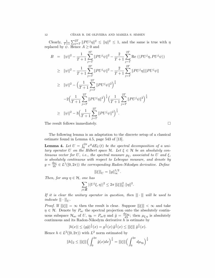
12 CESAR R. DE OLIVEIRA AND MARIZA S. SIMSEN
Clearly, 1T+1
∑2Tj=T ‖PU jη‖2 ≤ ‖η‖2 ≤ 1, and the same is true with η
replaced by ψ. Hence A ≥ 0 and
B = ‖ψ‖2 − 1T + 1
2T∑
j=T
‖PU jψ‖2 − 2T + 1
2T∑
j=T
Re (〈PU jη, PU jψ〉)
≥ ‖ψ‖2 − 1T + 1
2T∑
j=T
‖PU jψ‖2 − 2T + 1
2T∑
j=T
‖PU jη‖‖PU jψ‖
≥ ‖ψ‖2 −( 1
T + 1
2T∑
j=T
‖PU jψ‖2) 1
2
−2( 1
T + 1
2T∑
j=T
‖PU jη‖2) 1
2( 1
T + 1
2T∑
j=T
‖PU jψ‖2) 1
2
≥ ‖ψ‖2 − 3( 1
T + 1
2T∑
j=T
‖PU jψ‖2) 1
2.
The result follows immediately.
The following lemma is an adaptation to the discrete setup of a classicalestimate found in Lemma 4.5, page 543 of [13].
Lemma 4. Let U =∫ 2π0 eitdEU (t) be the spectral decomposition of a uni-
tary operator U on the Hilbert space H. Let ξ ∈ H be an absolutely con-tinuous vector for U , i.e., the spectral measure µξ, associated to U and ξ,is absolutely continuous with respect to Lebesgue measure, and denote byg = dµ#
dx ∈ L1([0, 2π)) the corresponding Radon-Nikodym derivative. Define
|‖ξ‖|U = ‖g‖1/2∞ .
Then, for any η ∈ H, one has∑
j∈ZZ
|〈U jξ, η〉|2 ≤ 2π |‖ξ‖|2U ‖η‖2.
If it is clear the unitary operator in question, then |‖ · ‖| will be used toindicate |‖ · ‖|U .
Proof. If |‖ξ‖| = ∞ then the result is clear. Suppose |‖ξ‖| < ∞ and takeη ∈ H. Denote by Pac the spectral projection onto the absolutely contin-uous subspace Hac of U , η0 = Pacη and g = dµ$0
dλ ; then µξ,η is absolutelycontinuous and its Radon-Nikodym derivative h is estimate by
|h(x)| ≤ (gg)12 (x) = g
12 (x) g
12 (x) ≤ |‖ξ‖| g
12 (x).
Hence h ∈ L2([0, 2π)) with L2 norm estimated by
‖h‖2 ≤ |‖ξ‖|( ∫ 2π
0g(x)dx
) 12 = |‖ξ‖|
( ∫ 2π
0dµη0
) 12

PURE POINT AND ENERGY INSTABILITY 13
= |‖ξ‖| · ‖η0‖ ≤ |‖ξ‖| · ‖η‖.
Since
〈U jξ, η〉 =∫ 2π
0eijtdµξ,η(t) =
∫ 2π
0eijth(t)dt =
√2π(Fh)(j),
it follows that∑
j∈ZZ
|〈U jξ, η〉|2 =∑
j∈ZZ
2π|(Fh)(j)|2 = 2π‖h‖22 ≤ 2π|‖ξ‖|2‖η‖2,
which is precisely the stated result.
4.2. Cauchy and Borel Transforms. Given a probability measure µ on∂D = z ∈ C : |z| = 1, its Cauchy Fµ(z) and Borel Rµ(z) transforms are,respectively, for z ∈ C with |z| 2= 1,
Fµ(z) =∫
∂D
eit + z
eit − zdµ(t)
and
Rµ(z) =∫
∂D
1eit − z
dµ(t).
Rµ is related to Fµ by
Fµ(z) = 2zRµ(z) + 1.(17)
Moreover, Fµ has the following properties [18]:• limr↑1 Fµ(reiθ) exists for a.e. θ, and if one decomposes the measure in
its absolutely continuous and singular parts
dµ(θ) = ω(θ)dθ
2π+ dµs(θ),
then
ω(θ) = limr↑1
Re Fµ(reiθ).(18)
• θ0 is a pure point of µ if and only if limr↑1(1 − r)Re Fµ(reiθ0) 2= 0.• dµs is supported on θ : limr↑1 Fµ(reiθ) = ∞.
Now, let U be a unitary operator on a separable Hilbert space H and φ acyclic vector for U . Consider the rank one perturbation of U
Uλ = UeiλP% = U(Id + (eiλ − 1)Pφ),
where Pφ(·) = 〈φ, ·〉φ and λ ∈ [0, 2π). Denote by dµλ the spectral measureassociated with Uλ and φ, Fλ = Fµ& and Rλ = Rµ& . We have the followingrelations between Rλ and R0, Fλ and F0:
14 CESAR R. DE OLIVEIRA AND MARIZA S. SIMSEN
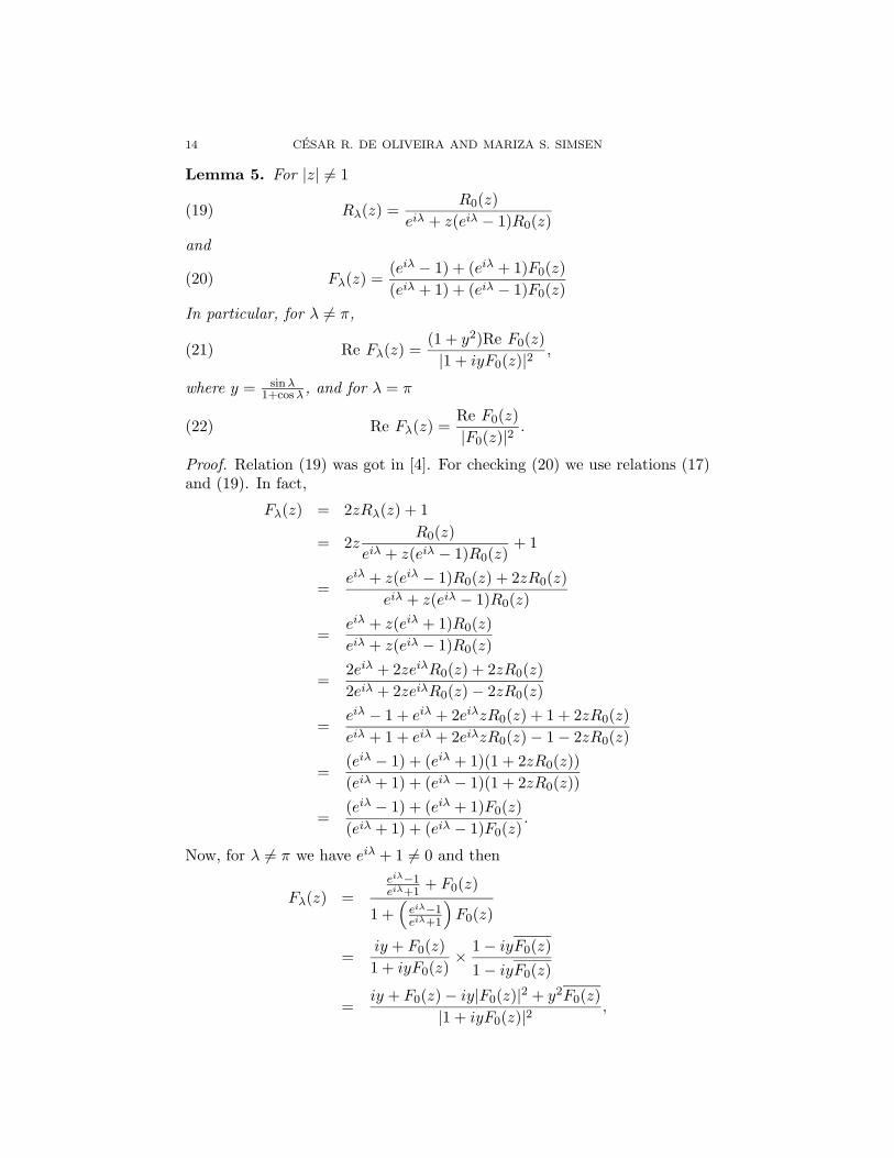
Lemma 5. For |z| 2= 1
Rλ(z) =R0(z)
eiλ + z(eiλ − 1)R0(z)(19)
and
Fλ(z) =(eiλ − 1) + (eiλ + 1)F0(z)(eiλ + 1) + (eiλ − 1)F0(z)
(20)
In particular, for λ 2= π,
Re Fλ(z) =(1 + y2)Re F0(z)|1 + iyF0(z)|2 ,(21)
where y = sinλ1+cosλ , and for λ = π
Re Fλ(z) =Re F0(z)|F0(z)|2 .(22)
Proof. Relation (19) was got in [4]. For checking (20) we use relations (17)and (19). In fact,
Fλ(z) = 2zRλ(z) + 1
= 2zR0(z)
eiλ + z(eiλ − 1)R0(z)+ 1
=eiλ + z(eiλ − 1)R0(z) + 2zR0(z)
eiλ + z(eiλ − 1)R0(z)
=eiλ + z(eiλ + 1)R0(z)eiλ + z(eiλ − 1)R0(z)
=2eiλ + 2zeiλR0(z) + 2zR0(z)2eiλ + 2zeiλR0(z) − 2zR0(z)
=eiλ − 1 + eiλ + 2eiλzR0(z) + 1 + 2zR0(z)eiλ + 1 + eiλ + 2eiλzR0(z) − 1 − 2zR0(z)
=(eiλ − 1) + (eiλ + 1)(1 + 2zR0(z))(eiλ + 1) + (eiλ − 1)(1 + 2zR0(z))
=(eiλ − 1) + (eiλ + 1)F0(z)(eiλ + 1) + (eiλ − 1)F0(z)
.
Now, for λ 2= π we have eiλ + 1 2= 0 and then
Fλ(z) =ei&−1ei&+1
+ F0(z)
1 +(
ei&−1ei&+1
)F0(z)
=iy + F0(z)1 + iyF0(z)
× 1 − iyF0(z)1 − iyF0(z)
=iy + F0(z) − iy|F0(z)|2 + y2F0(z)
|1 + iyF0(z)|2 ,

PURE POINT AND ENERGY INSTABILITY 15
where ei&−1ei&+1
= iy and y = sinλ1+cosλ . So, for λ 2= π,
Re Fλ(z) =(1 + y2)Re F0(z)|1 + iyF0(z)|2
and (21) is obtained. For λ = π we have Fλ(z) = 1F0(z) and (22) follows.
Lemma 6. Fix a rational number β. Then there exist C1 > 0 and C2 < ∞,and for each θ ∈ [0, 2π) and λ ∈ [π6 , π2 ] a decomposition
ϕ1 = ηθ,λ + ψθ,λ
so that
〈ηθ,λ,ψθ,λ〉 = 0,(23)
‖ψθ,λ‖ ≥ C1,(24)
|‖ψθ,λ‖|U&(β,θ)+ ≤ C2(25)
(the notation |‖ · ‖|U was introduced in Lemma 4).
Proof. We break the proof in some steps.Step 1. By Theorem 1, since β is rational,
σsc(U(β, θ)+) = ∅, σac(U(β, θ)+) = σac(U(β, θ))
and the point spectrum of U(β, θ)+ consists of finitely many simple eigen-values in the resolvent set of U(β, θ). Denote by µθ,λ the spectral measureassociated to Uλ(β, θ)+ and (the cyclic vector) ϕ1, and by µθ the spectralmeasure associated to U(β, θ)+ and ϕ1 (i.e., the case λ = 0). Write
dµθ,λ(E) = fθ,λ(E)dE
2π+ dµθ,λs (E),
dµθ(E) = fθ(E)dE
2π+ dµθp(E).
Step 2. Relation between fθ,λ and fθ: By Lemma 5, for λ 2= π one has
Re Fµ",&(z) =(1 + y2)Re Fµ"(z)|1 + iyFµ"(z)|2
,
where y = sinλ1+cosλ and then
fθ,λ(E) =(1 + y2)fθ(E)
|1 + iy limr↑1 Fµ"(reiE)|2,
for almost all E.
Step 3. Relation between fθ and f0: By (9) and (8) one gets
U(β, θ)+ = e−i2θU(β, 0)+(26)

16 CESAR R. DE OLIVEIRA AND MARIZA S. SIMSEN
and using this relation it found that(U(β, θ)+
)j = e−ij2θ(U(β, 0)+
)j
for all j ∈ ZZ. Thus, by the spectral theorem, for any j ∈ ZZ,∫ 2π
0e−ijEfθ(E)
dE
2π=
∫ 2π
0e−ijEf0(E − 2θ)
dE
2π.
Hence
fθ(E) = f0(E − 2θ)(27)
for almost all E.
Step 4. Lower and upper bounds for fθ,λ: We have
limr↑1
Fµ"(reiE) = fθ(E) + i lim
r↑1Im Fµ"(re
iE)
and
limr↑1
Im Fµ"(reiE) = lim
r↑1
∫ 2π
0Im
(eit + reiE
eit − reiE
)fθ(t)
dt
2π
+ limr↑1
∫ 2π
0Im
(eit + reiE
eit − reiE
)dµθp(t).
If we denote
gθ(E) = limr↑1
∫ 2π
0Im
(eit + reiE
eit − reiE
)fθ(t)
dt
2π,
then by (27) we obtain gθ(E) = g0(E − 2θ) for almost all E. On the otherhand, by (26) we have that E is an eigenvalue of U(β, θ)+ if and only ifE − 2θ is an eigenvalue of U(β, 0)+. Let Eθ
j nj=1 be the set of eigenvalues
of U(β, θ)+ (recall that n < ∞) and dµθp =∑n
j=1 κθjδE"
j(δE is the Dirac
measure at E). Then
limr↑1
∫ 2π
0Im
(eit + reiE
eit − reiE
)dµθp(t) = lim
r↑1
∫ 2π
0
2r sin(E − t)1 + r2 − 2r cos(E − t)
dµθp(t)
= limr↑1
n∑
j=1
2r sin(E − Eθj )κθj
1 + r2 − 2r cos(E − Eθj )
=n∑
j=1
2 sin(E − 2θ − E0j )κθj∣∣∣eiE0
j − ei(E−2θ)∣∣∣2 .
Since f0 ∈ L1([0, 2π)), by a result of [14] (Theorem 1.6 in Chapter III),the function g0 is of weak L1 type, i.e., g0 is measurable and there exits aconstant C > 0 such that for all T > 0 the Lebesgue measure
|E : |g0(E)| ≤ T| ≥ 1 − C
T.(28)

PURE POINT AND ENERGY INSTABILITY 17
Pick S > 0 such that ΩS :=
E : 1S ≤ f0(E) ≤ S
satisfies |ΩS | > 0 and
dist (ΩS , E0j n
j=1) = L > 0. Then choose T sufficiently large such that
A := ΩS ∩ E : |g0(E)| ≤ T
satisfies |A| > 0; by (28) this is possible. For θ ∈ [0, 2π) put
Iθ := E ∈ [0, 2π) : E − 2θ ∈ A;
thus |Iθ| = |A| > 0. Then, for all θ ∈ [0, 2π), λ ∈ [0, π2 ] (equivalentlyy ∈ [0, 1]) and almost all E ∈ Iθ one has
∣∣∣∣1 + iy limr↑1
Fµ"(reiE)
∣∣∣∣ ≤ 1 + |y|(
fθ(E) + |gθ(E)|
+
∣∣∣∣∣∣
n∑
j=1
2 sin(E − 2θ − E0j )κθj
|eiE0j − ei(E−2θ)|2
∣∣∣∣∣∣
)
≤ 1 + f0(E − 2θ) + |g0(E − 2θ)| +n∑
j=1
2|κθj |L2
≤ 1 + S + T +2L2
.
So, for all θ ∈ [0, 2π), λ ∈ [0, π2 ] and almost all E ∈ Iθ
fθ,λ(E) =(1 + y2)fθ(E)
|1 + iy limr↑1 Fµ"(reiE))|2
≥ f0(E − 2θ)(1 + S + T + 2/L2)2
≥ 1S(1 + S + T + 2/L2)2
.
In order to get un upper bound, note that∣∣∣∣1 + iy lim
r↑1Fµ"(re
iE)∣∣∣∣ ≥ yfθ(E) ≥ 0,
and so, for all θ ∈ [0, 2π), λ ∈ [π6 , π2 ] (equivalently y ∈[
12+
√3, 1
]) and almost
all E ∈ Iθ
fθ,λ(E) =(1 + y2)fθ(E)
|1 + iy limr↑1 Fµ"(reiE)|2
≤ (1 + y2)fθ(E)y2fθ(E)2
=(1 + y2)
y2f0(E − 2θ)≤ 2(2 +
√3)2S.

18 CESAR R. DE OLIVEIRA AND MARIZA S. SIMSEN
Summing up, for all θ ∈ [0, 2π), λ ∈ [π6 , π2 ] and almost all E ∈ Iθ, we haveproved that
1S(1 + S + T + 2/L2)2
≤ fθ,λ(E) ≤ 2(2 +√
3)2S.(29)
Step 5. Conclusion: For λ ∈ [π6 , π2 ] and θ ∈ [0, 2π) let
ψθ,λ = P θ,λI"
ϕ1, ηθ,λ = (Id − P θ,λI"
)ϕ1,
where P θ,λI"
is the spectral projection (of Uλ(β, θ)+) onto Iθ. Then for eachθ ∈ [0, 2π) and λ ∈ [π6 , π2 ] we have the decomposition ϕ1 = ψθ,λ + ηθ,λ thatsatisfies (23).
By the construction in Step 4, we have that A = I0 is in the absolutelycontinuous spectrum of U(β, 0)+, so by (26) and the definition of Iθ it fol-lows that Iθ is in the absolutely continuous spectrum of U(β, θ)+; thususing Birman-Krein’s theorem on invariance of absolutely continuous spec-trum under trace class perturbations, we conclude that Iθ belongs to theabsolutely continuous spectrum of Uλ(β, θ)+ for all λ. Therefore by (29)
‖ψθ,λ‖2 = 〈ψθ,λ,ψθ,λ〉 = 〈P θ,λI"
ϕ1, Pθ,λI"
ϕ1〉
= 〈ϕ1, Pθ,λI"
ϕ1〉 =∫ 2π
0χI"(E)dµθ,λ
=∫
I"
fθ,λ(E)dE
2π≥ |A|
2πS(1 + S + T + 2/L2)2
and (24) holds with
C1 =( |A|
2πS(1 + S + T + 2/L2)2)1/2
> 0;
also
|‖ψθ,λ‖|2U&(β,θ)+ = |‖P θ,λI"
ϕ1‖|2
U&(β,θ)+= ‖χI"fθ,λ‖∞ ≤ 2(2 +
√3)2S
and (25) holds with C2 = (2(2 +√
3)2S)1/2 < ∞. The lemma is proved.
4.3. Variation of β. The next lemma gives an estimate of the dependenceof the dynamics on β. Its proof strongly uses the structure of Uλ(β, θ)+.
Lemma 7. Let β,β′ ∈ IR. Then, for n ≥ 1,∥∥(
Uλ(β, θ)+)n
ϕ1 −(Uλ(β′, θ)+
)nϕ1
∥∥ ≤ 2 × 4n(2n2 − n)2π∣∣β − β′∣∣ .

PURE POINT AND ENERGY INSTABILITY 19
Proof. It is an induction. We have
Uλ(β, θ)+ϕj = U(β, θ)+(Id + (eiλ − 1)Pϕ1)ϕj
=
U(β, θ)+ϕj if j > 1U(β, θ)+ϕ1 + (eiλ − 1)U(β, θ)+ϕ1 if j = 1
=
U(β, θ)+ϕj if j > 1eiλU(β, θ)+ϕ1 if j = 1
Thus
Uλ(β, θ)+ϕ1 = eiλU(β, θ)+ϕ1 = a1e−i(2πβ)ϕ1 + a2e
−i(2πβ)ϕ2
where a1 = reiλe−i(α+2θ) and a2 = iteiλe−i(α+2θ). Since
|e−ix − e−ix# | ≤ 2|x − x′|(30)
and |aj | ≤ 1, j = 1, 2, then
∥∥Uλ(β, θ)+ϕ1 − Uλ(β′, θ)+ϕ1
∥∥ ≤ 2∣∣∣e−i(2πβ) − e−i(2πβ#)
∣∣∣
≤ 4 × 2|2πβ − 2πβ′| = 2 × 4 × 2π∣∣β − β′∣∣
and the lemma is proved for n = 1.Now(Uλ(β, θ)+
)2ϕ1 = Uλ(β, θ)+Uλ(β, θ)+ϕ1
= Uλ(β, θ)+(a1e−i(2πβ)ϕ1 + a2e
−i(2πβ)ϕ2)= eiλa1e
−i(2πβ)U(β, θ)+ϕ1 + a2e−i(2πβ)U(β, θ)+ϕ2
= eiλa1e−i(2πβ)
(b1e
−i(2πβ)ϕ1 + b2e−i(2πβ)ϕ2
)
+a2e−i(2πβ)
(c1e
−i(3.(2πβ))ϕ1 + c2e−i(3.(2πβ))ϕ2
+c3e−i(5.(2πβ))ϕ3 + c4e
−i(5.(2πβ))ϕ4
)
Since |aj | < 1, |bj | < 1, |cj | < 1 and there are 2 + 4 < 4 × 4 terms in theexpansion of (Uλ(β, θ)+)2 ϕ1 and the largest exponent (which provides thelargest contribution by (30)) is obtained from the product of the exponentialse−i(2πβ)e−i((2+3)2πβ) = e−i((1+2+3)2πβ), we obtain∥∥∥(Uλ(β, θ)+
)2ϕ1 −
(Uλ(β′, θ)+
)2ϕ1
∥∥∥ ≤ 4 × 4 × 2(1 + 2 + 3)2π∣∣β − β′∣∣
= 2 × 42(1 + 2 + 3)2π∣∣β − β′∣∣ ,
and the lemma is proved for n = 2. In a similar way by the structure ofUλ(β, θ)+ we conclude that (Uλ(β, θ)+)3 ϕ1 has at most 42 × 4 terms wherethe largest exponent is in e−i(1+2+3)2πβe−i((4+5)2πβ) = e−i((1+2+3+4+5)2πβ)

20 CESAR R. DE OLIVEIRA AND MARIZA S. SIMSEN
and so ∥∥∥(Uλ(β, θ)+
)3ϕ1 −
(Uλ(β′, θ)+
)3ϕ1
∥∥∥ ≤
≤ 4 × 4 × 4 × 2(1 + 2 + 3 + 4 + 5)2π∣∣β − β′∣∣
= 2 × 43(1 + 2 + 3 + 4 + 5)2π∣∣β − β′∣∣ .
Inductively one finds that (Uλ(β, θ)+)n ϕ1 has at the most 4n terms, andaccording to (30) the largest contribution comes from the product
e−i(1+2+...+2n−3)2πβe−i(((2n−2)+(2n−1))2πβ) = e−i((1+2+...+2n−1)2πβ)
and then∥∥(
Uλ(β, θ)+)n
ϕ1 −(Uλ(β′, θ)+
)nϕ1
∥∥
≤ 2 × 4n(1 + 2 + . . . + 2n − 1)2π∣∣β − β′∣∣ ;
since 2n2 − n = 1 + 2 + . . . + 2n − 1, the result follows.
4.4. Proof of Theorem 2(ii). Finally, using this preparatory set of results,we finish the proof of our main result.
Let f(n) = (ln(2+ |n|))15 . Sequences βm, Tm,∆m will be built inductively,
starting with β1 = 1, so that(i) βm+1 − βm = 2−κm! for some κm ∈ IN;(ii) 1
Tm+1
∑2Tmj=Tm
‖Pn≥ Tmf(Tm)
(Uλ(β, θ)+)j ϕ1‖2 ≥ 1f(Tm)2 for all θ ∈ [0, 2π),
λ ∈ [π6 , π2 ] and β with |β − βm| ≤ ∆m;(iii) |βm+1 − βk| < ∆k for k = 1, 2, . . . , m.
If (i), (ii) and (iii) are satisfied then we conclude by (i) that β∞ = limβm
is irrational, by (iii) that |β∞ − βm| ≤ ∆m and then by (ii) that
1Tm + 1
2Tm∑
j=Tm
‖Pn≥ Tmf(Tm)
(Uλ(β∞, θ)+
)jϕ1‖2 ≥ 1
f(Tm)2
for θ ∈ [0, 2π) and λ ∈ [π6 , π2 ]. So by Lemma 2
lim supn→∞
‖X(Uλ(β, θ)+
)nϕ1‖2 f(n)5
n2= ∞
for β = β∞ and the result is proved.Then we shall construct βm, Tm,∆m such that (i), (ii) and (iii) hold. Start
with β1 = 1. Given β1, . . . ,βm, T1, . . . , Tm−1 and ∆1, . . . ,∆m−1 we shallshow how to choose Tm,∆m and βm+1.
Given βm, let ϕ1 = η+ψ be the decomposition given by Lemma 6 and letC1, C2 be the corresponding constants. Choose Tm ≥ 2Tm−1 (and T1 ≥ 2)so that
C21 − 3
√2πC2(2f(Tm)−1 + T−1
m )12 ≥ 2f(Tm)−1.(31)

PURE POINT AND ENERGY INSTABILITY 21
This is possible since C1 and C2 are fixed (given βm) and f(n) → ∞.Note that
1T + 1
2T∑
j=T
‖Pn< Tf(T )
(Uλ(β, θ)+
)jψ‖2 ≤ 2π
T + 1#
n : n <
T
f(T )
|‖ψ‖|2;
(32)
in fact
1T + 1
2T∑
j=T
‖Pn< Tf(T )
(Uλ(β, θ)+
)jψ‖2 =
=1
T + 1
2T∑
j=T
∑
n< Tf(T )
∣∣∣((
Uλ(β, θ)+)j
ψ)
(n)∣∣∣2
=1
T + 1
∑
n< Tf(T )
2T∑
j=T
∣∣∣((
Uλ(β, θ)+)j
ψ)
(n)∣∣∣2
≤ 1T + 1
∑
n< Tf(T )
∞∑
j=−∞
∣∣∣〈ϕn,(Uλ(β, θ)+
)jψ〉
∣∣∣2,
then by Lemma 4
1T + 1
2T∑
j=T
‖Pn< Tf(T )
(Uλ(β, θ)+
)jψ‖2 ≤ 1
T + 1
∑
n< Tf(T )
2π|‖ψ‖|2,
and (32) follows.By Lemma 3 and (32)
1Tm + 1
2Tm∑
j=Tm
‖Pn≥ Tmf(Tm)
(Uλ(βm, θ)+
)jϕ1‖2 ≥
≥ ‖ψ‖2 − 3( 1
Tm + 1
2Tm∑
j=Tm
‖Pn< Tmf(Tm)
(Uλ(βm, θ)+
)jψ‖2
) 12
≥ ‖ψ‖2 − 3( 2π
Tm + 1#
n : n <
Tm
f(Tm)
|‖ψ‖|2
) 12
≥ C21 − 3
( 2πTm + 1
#
n : n <Tm
f(Tm)
C2
2
) 12
= C21 − 3
√2πC2
( 1Tm + 1
#
n : n <Tm
f(Tm)
) 12.

22 CESAR R. DE OLIVEIRA AND MARIZA S. SIMSEN
Since #
n : n < Tmf(Tm)
≤ 2 Tm
f(Tm) + 1 it follows that
1Tm + 1
2Tm∑
j=Tm
‖Pn≥ Tmf(Tm)
(Uλ(βm, θ)+
)jϕ1‖2
≥ C21 − 3
√2πC2
( 1Tm + 1
( 2Tm
f(Tm)+ 1
)) 12
≥ C21 − 3
√2πC2
( 2f(Tm)
+1
Tm
) 12
for θ ∈ [0, 2π) and λ ∈ [π6 , π2 ]. Thus by (31), we obtain
1Tm + 1
2Tm∑
j=Tm
‖Pn≥ Tmf(Tm)
(Uλ(βm, θ)+
)jϕ1‖2 ≥ 2
f(Tm)
for θ ∈ [0, 2π) and λ ∈ [π6 , π2 ].So, by Lemma 7, for β ∈ IR, θ ∈ [0, 2π) and λ ∈ [π6 , π2 ]
1Tm + 1
2Tm∑
j=Tm
‖Pn≥ Tmf(Tm)
(Uλ(β, θ)+
)jϕ1‖2 ≥
≥( 1
Tm + 1
2Tm∑
j=Tm
‖P|n|≥ Tmf(Tm)
(Uλ(β, θ)+
)jϕ1‖
)2
=
(1
Tm + 1
2Tm∑
j=Tm
∥∥∥Pn≥ Tmf(Tm)
(Uλ(βm, θ)+
)jϕ1
+Pn≥ Tmf(Tm)
((Uλ(β, θ)+
)jϕ1 −
(Uλ(βm, θ)+
)jϕ1
) ∥∥∥
)2
≥(
1Tm + 1
2Tm∑
j=Tm
∥∥∥∥Pn≥ Tmf(Tm)
(Uλ(βm, θ)+
)jϕ1
∥∥∥∥
−∥∥∥((
Uλ(β, θ)+)j −
(Uλ(βm, θ)+
)j)ϕ1
∥∥∥
)2
≥( 1
Tm + 1
2Tm∑
j=Tm
(‖Pn≥ Tmf(Tm)
(Uλ(βm, θ)+
)jϕ1‖2
−4j+1(2j2 − j)π|β − βm|))2
≥( 2
f(Tm)− 1
Tm + 1
( 2Tm∑
j=Tm
4j+1(2j2 − j)π)|β − βm|
)2.
PURE POINT AND ENERGY INSTABILITY 23
Taking
∆m =Tm + 1
f(Tm)∑2Tm
j=Tm4j+1(2j2 − j)π
we obtain that, if |β − βm| < ∆m,
1Tm + 1
2Tm∑
j=Tm
‖Pn≥ Tmf(Tm)
(Uλ(β, θ)+
)jϕ1‖2 ≥ 1
f(Tm)2.
Finally, pick βm+1 rational so that
|βn − βm+1| < ∆n n = 1, . . . , m,
and βm+1 = βm + 2−κm! for some κm ∈ IN. This finishes the proof ofTheorem 2(ii).
Remark. For the operator Uλ(β, θ) := U(β, θ)(Id +(eiλ−1)Pϕ1) on l2(ZZ) wecan similarly prove an analogous result. The proof of dynamical instabilityfor some irrational β is essentially unchanged except for Lemma 6 which issimplified since U(β, θ) is purely absolutely continuous for β rational. Onthe other hand, about pure point spectrum, the main difference in this caseis that ϕ1 might not be cyclic, an thus, we don’t get pure point spectrumfor Uλ(β, θ) for a.e. θ and λ as obtained on l2(IN∗), but we get that ϕ1 is inthe point spectral subspace corresponding to Uλ(β, θ) for a.e. θ and λ.
References
[1] Blatter G., Browne D.: Zener Tunneling and Localization in small Conducting Rings.Phys. Rev. B 37, 3856–3880 (1988)
[2] Bourget O.: Singular Continuous Floquet Operator for Periodic Quantum Systems.J. Math. Anal. Appl. 301, 65–83 (2005)
[3] Bourget O., Howland J. S., Joye A.: Spectral Analysis of Unitary Band Matrices.Commun. Math. Phys. 234, 191–227 (2003)
[4] Combescure M.: Spectral Properties of a Periodically Kicked Quantum Hamiltonian.J. Stat. Phys. 59, 679–690 (1990)
[5] Cycon H. L., Froese R. G., Kirsch W., Simon B.: Schrodinger Operators. Berlin:Springer-Verlag, 1987
[6] de Oliveira C. R., Prado R. A.: Spectral and Localization Properties for the One-Dimensional Bernoulli Discrete Dirac Operator. J. Math. Phys. 46, 072105 (2005)
[7] del Rio R., Jitomirskaya S., Last Y., Simon B.: Operators with Singular ContinuousSpectrum IV: Hausdor! Dimensions, Rank One Perturbations and Localization. J.d’Analyse Math. 69, 153–200 (1996)
[8] Enss V., Veselic K.: Bound States and Propagating States for Time-DependentHamiltonians. Ann. Inst. H. Poincare Sect. A 39, 159–191 (1983)
[9] Hamza E., Joye A., Stolz G.: Localization for Random Unitary Operators. Lett.Math. Phys. 75, 255–272 (2006)
[10] Jitomirskaya S., Schulz-Baldes H., Stolz G.: Delocalization in Random Polymer Mod-els. Commun. Math. Phys. 233, 27–48 (2003)
[11] Joye A.: Density of States and Thouless Formula for Random Unitary Band Matrices.Ann. Henri Poincare 5, 347–379 (2004)

24 CESAR R. DE OLIVEIRA AND MARIZA S. SIMSEN
[12] Joye A.: Fractional Moment Estimates for Random Unitary Band Matrices. Lett.Math. Phys. 72, 51–64 (2005)
[13] Kato T.: Perturbation Theory for Linear Operators—Second Edition. Berlin:Springer-Verlag, 1980
[14] Katznelson Y.: An Introduction to Harmonic Analysis. New York: John Wiley, 1968[15] Reed M., Simon B.: Methods of Modern Mathematical Physics III Scattering Theory.
New York: Acad. Press 1979[16] Simon B.: Absence of Ballistic Motion. Commun. Math. Phys. 134, 209–212 (1990)[17] Simon B.: Spectral Analysis of rank one Perturbations and Applications. CRM Lec-
ture Notes Vol. 8, 109–149 (1995) (J. Feldman, R. Froese, L. Rosen, eds.)[18] Simon B.: Analogs of the M-Function in the Theory of Orthogonal Polynomials on
the Unit Circle. J. Comput. Appl. Math. 171, 411–424 (2004)[19] Simon B.: Aizenman’s Theorem for Orthogonal Polynomials On the Unit Circle.
Constr. Approx. 23, 229–240 (2006)[20] Simon B., Wolf T.: Singular Continuous Spectrum under rank one Perturbations
and Localization for Random Hamiltonians. Commun. Pure Appl. Math. 39, 75–90(1986)
Departamento de Matematica – UFSCar, Sao Carlos, SP, 13560-970 BrazilE-mail address: [email protected]
Departamento de Matematica – UFSCar, Sao Carlos, SP, 13560-970 BrazilE-mail address: [email protected]

![All Hands offers opera students a unique on Deck ...€¦ · We had Maestro James Conlon [music direc-tor of LA Opera] in residence for a master class and to help celebrate the Opera](https://img.pdfslide.us/doc/110x75/610553fd2b2e1a29861347e0/all-hands-offers-opera-students-a-unique-on-deck-we-had-maestro-james-conlon.jpg)