A Flexible New Technique for CameraCalibration

Zhengyou Zhang

December 2, 1998(updated on December 14, 1998)

(updated on March 25, 1999)(updated on Aug. 10, 2002; a typo in Appendix B)

(last updated on Aug. 13, 2008; a typo in Section 3.3)

Technical ReportMSR-TR-98-71

Microsoft ResearchMicrosoft Corporation

One Microsoft WayRedmond, WA 98052

zhang@microsoft.comhttp://research.microsoft.com/˜zhang

A Flexible New Technique for Camera Calibration

Zhengyou ZhangMicrosoft Research, One Microsoft Way, Redmond, WA 98052-6399, USA

zhang@microsoft.com http://research.microsoft.com/˜zhang

Contents

1 Motivations 2

2 Basic Equations 32.1 Notation . . . . . . . . . . . . . . . . . . . . . . . . . . . . . . . . . . . . . . . . . 32.2 Homography between the model plane and its image . . . . . . . . . . . . . . . . . 42.3 Constraints on the intrinsic parameters . . . . . . . . . . . . . . . . . . . . . . . . . 42.4 Geometric Interpretation† . . . . . . . . . . . . . . . . . . . . . . . . . . . . . . . . 4

3 Solving Camera Calibration 53.1 Closed-form solution . . . . . . . . . . . . . . . . . . . . . . . . . . . . . . . . . . 53.2 Maximum likelihood estimation . . . . . . . . . . . . . . . . . . . . . . . . . . . . 63.3 Dealing with radial distortion . . . . . . . . . . . . . . . . . . . . . . . . . . . . . . 73.4 Summary . . . . . . . . . . . . . . . . . . . . . . . . . . . . . . . . . . . . . . . . 8

4 Degenerate Configurations 8

5 Experimental Results 95.1 Computer Simulations . . . . . . . . . . . . . . . . . . . . . . . . . . . . . . . . . 95.2 Real Data . . . . . . . . . . . . . . . . . . . . . . . . . . . . . . . . . . . . . . . . 105.3 Sensitivity with Respect to Model Imprecision‡ . . . . . . . . . . . . . . . . . . . . 14

5.3.1 Random noise in the model points . . . . . . . . . . . . . . . . . . . . . . . 145.3.2 Systematic non-planarity of the model pattern . . . . . . . . . . . . . . . . . 15

6 Conclusion 17

A Estimation of the Homography Between the Model Plane and its Image 17

B Extraction of the Intrinsic Parameters from Matrix B 18

C Approximating a 3× 3 matrix by a Rotation Matrix 18

D Camera Calibration Under Known Pure Translation§ 19

†added on December 14, 1998‡added on December 28, 1998; added results on systematic non-planarity on March 25, 1998§added on December 14, 1998, corrected (based on the comments from Andrew Zisserman) on January 7, 1999

1

A Flexible New Technique for Camera Calibration

Abstract

We propose a flexible new technique to easily calibrate a camera. It is well suited for usewithout specialized knowledge of 3D geometry or computer vision. The technique only requiresthe camera to observe a planar pattern shown at a few (at least two) different orientations. Eitherthe camera or the planar pattern can be freely moved. The motion need not be known. Radial lensdistortion is modeled. The proposed procedure consists of a closed-form solution, followed by anonlinear refinement based on the maximum likelihood criterion. Both computer simulation andreal data have been used to test the proposed technique, and very good results have been obtained.Compared with classical techniques which use expensive equipment such as two or three orthog-onal planes, the proposed technique is easy to use and flexible. It advances 3D computer visionone step from laboratory environments to real world use.

Index Terms— Camera calibration, calibration from planes, 2D pattern, absolute conic, projectivemapping, lens distortion, closed-form solution, maximum likelihood estimation, flexible setup.

1 Motivations

Camera calibration is a necessary step in 3D computer vision in order to extract metric informationfrom 2D images. Much work has been done, starting in the photogrammetry community (see [2,4] to cite a few), and more recently in computer vision ([9, 8, 23, 7, 26, 24, 17, 6] to cite a few).We can classify those techniques roughly into two categories: photogrammetric calibration and self-calibration.

Photogrammetric calibration. Camera calibration is performed by observing a calibration objectwhose geometry in 3-D space is known with very good precision. Calibration can be done veryefficiently [5]. The calibration object usually consists of two or three planes orthogonal to eachother. Sometimes, a plane undergoing a precisely known translation is also used [23]. Theseapproaches require an expensive calibration apparatus, and an elaborate setup.

Self-calibration. Techniques in this category do not use any calibration object. Just by moving acamera in a static scene, the rigidity of the scene provides in general two constraints [17, 15]on the cameras’ internal parameters from one camera displacement by using image informa-tion alone. Therefore, if images are taken by the same camera with fixed internal parameters,correspondences between three images are sufficient to recover both the internal and externalparameters which allow us to reconstruct 3-D structure up to a similarity [16, 13]. While this ap-proach is very flexible, it is not yet mature [1]. Because there are many parameters to estimate,we cannot always obtain reliable results.

Other techniques exist: vanishing points for orthogonal directions [3, 14], and calibration from purerotation [11, 21].

Our current research is focused on a desktop vision system (DVS) since the potential for usingDVSs is large. Cameras are becoming cheap and ubiquitous. A DVS aims at the general public,who are not experts in computer vision. A typical computer user will perform vision tasks only fromtime to time, so will not be willing to invest money for expensive equipment. Therefore, flexibility,robustness and low cost are important. The camera calibration technique described in this paper wasdeveloped with these considerations in mind.

2

The proposed technique only requires the camera to observe a planar pattern shown at a few (atleast two) different orientations. The pattern can be printed on a laser printer and attached to a “rea-sonable” planar surface (e.g., a hard book cover). Either the camera or the planar pattern can be movedby hand. The motion need not be known. The proposed approach lies between the photogrammet-ric calibration and self-calibration, because we use 2D metric information rather than 3D or purelyimplicit one. Both computer simulation and real data have been used to test the proposed technique,and very good results have been obtained. Compared with classical techniques, the proposed tech-nique is considerably more flexible. Compared with self-calibration, it gains considerable degree ofrobustness. We believe the new technique advances 3D computer vision one step from laboratoryenvironments to the real world.

Note that Bill Triggs [22] recently developed a self-calibration technique from at least 5 views ofa planar scene. His technique is more flexible than ours, but has difficulty to initialize. Liebowitz andZisserman [14] described a technique of metric rectification for perspective images of planes usingmetric information such as a known angle, two equal though unknown angles, and a known lengthratio. They also mentioned that calibration of the internal camera parameters is possible provided atleast three such rectified planes, although no experimental results were shown.

The paper is organized as follows. Section 2 describes the basic constraints from observing asingle plane. Section 3 describes the calibration procedure. We start with a closed-form solution,followed by nonlinear optimization. Radial lens distortion is also modeled. Section 4 studies con-figurations in which the proposed calibration technique fails. It is very easy to avoid such situationsin practice. Section 5 provides the experimental results. Both computer simulation and real data areused to validate the proposed technique. In the Appendix, we provides a number of details, includingthe techniques for estimating the homography between the model plane and its image.

2 Basic Equations

We examine the constraints on the camera’s intrinsic parameters provided by observing a single plane.We start with the notation used in this paper.

2.1 Notation

A 2D point is denoted by m = [u, v]T . A 3D point is denoted by M = [X,Y, Z]T . We use x to denotethe augmented vector by adding 1 as the last element: m = [u, v, 1]T and M = [X, Y, Z, 1]T . A camerais modeled by the usual pinhole: the relationship between a 3D point M and its image projection m isgiven by

sm = A[R t

]M , (1)

where s is an arbitrary scale factor, (R, t), called the extrinsic parameters, is the rotation and trans-lation which relates the world coordinate system to the camera coordinate system, and A, called thecamera intrinsic matrix, is given by

A =

α γ u0

0 β v0

0 0 1

with (u0, v0) the coordinates of the principal point, α and β the scale factors in image u and v axes,and γ the parameter describing the skewness of the two image axes.

We use the abbreviation A−T for (A−1)T or (AT )−1.

3

2.2 Homography between the model plane and its image

Without loss of generality, we assume the model plane is on Z = 0 of the world coordinate system.Let’s denote the ith column of the rotation matrix R by ri. From (1), we have

s

uv1

= A

[r1 r2 r3 t

]

XY01

= A[r1 r2 t

]

XY1

.

By abuse of notation, we still use M to denote a point on the model plane, but M = [X, Y ]T since Z isalways equal to 0. In turn, M = [X, Y, 1]T . Therefore, a model point M and its image m is related by ahomography H:

sm = HM with H = A[r1 r2 t

]. (2)

As is clear, the 3× 3 matrix H is defined up to a scale factor.

2.3 Constraints on the intrinsic parameters

Given an image of the model plane, an homography can be estimated (see Appendix A). Let’s denoteit by H =

[h1 h2 h3

]. From (2), we have

[h1 h2 h3

]= λA

[r1 r2 t

],

where λ is an arbitrary scalar. Using the knowledge that r1 and r2 are orthonormal, we have

hT1 A−TA−1h2 = 0 (3)

hT1 A−TA−1h1 = hT

2 A−TA−1h2 . (4)

These are the two basic constraints on the intrinsic parameters, given one homography. Because ahomography has 8 degrees of freedom and there are 6 extrinsic parameters (3 for rotation and 3 fortranslation), we can only obtain 2 constraints on the intrinsic parameters. Note that A−TA−1 actuallydescribes the image of the absolute conic [16]. In the next subsection, we will give an geometricinterpretation.

2.4 Geometric Interpretation

We are now relating (3) and (4) to the absolute conic.It is not difficult to verify that the model plane, under our convention, is described in the camera

coordinate system by the following equation:[

r3

rT3 t

]T [xyzw

]= 0 ,

where w = 0 for points at infinity and w = 1 othewise. This plane intersects the plane at infinity at a

line, and we can easily see that[r1

0

]and

[r2

0

]are two particular points on that line. Any point on it

4

is a linear combination of these two points, i.e.,

x∞ = a

[r1

0

]+ b

[r2

0

]=

[ar1 + br2

0

].

Now, let’s compute the intersection of the above line with the absolute conic. By definition, thepoint x∞, known as the circular point, satisfies: xT∞x∞ = 0, i.e.,

(ar1 + br2)T (ar1 + br2) = 0, or a2 + b2 = 0 .

The solution is b = ±ai, where i2 = −1. That is, the two intersection points are

x∞ = a

[r1 ± ir2

0

].

Their projection in the image plane is then given, up to a scale factor, by

m∞ = A(r1 ± ir2) = h1 ± ih2 .

Point m∞ is on the image of the absolute conic, described by A−TA−1 [16]. This gives

(h1 ± ih2)TA−TA−1(h1 ± ih2) = 0 .

Requiring that both real and imaginary parts be zero yields (3) and (4).

3 Solving Camera Calibration

This section provides the details how to effectively solve the camera calibration problem. We startwith an analytical solution, followed by a nonlinear optimization technique based on the maximumlikelihood criterion. Finally, we take into account lens distortion, giving both analytical and nonlinearsolutions.

3.1 Closed-form solution

Let

B = A−TA−1 ≡

B11 B12 B13

B12 B22 B23

B13 B23 B33

=

1α2 − γ

α2βv0γ−u0β

α2β

− γα2β

γ2

α2β2 + 1β2 −γ(v0γ−u0β)

α2β2 − v0β2

v0γ−u0βα2β

−γ(v0γ−u0β)α2β2 − v0

β2(v0γ−u0β)2

α2β2 + v20

β2 +1

. (5)

Note that B is symmetric, defined by a 6D vector

b = [B11, B12, B22, B13, B23, B33]T . (6)

Let the ith column vector of H be hi = [hi1, hi2, hi3]T . Then, we have

hTi Bhj = vT

ijb (7)

5

with

vij = [hi1hj1, hi1hj2 + hi2hj1, hi2hj2,

hi3hj1 + hi1hj3, hi3hj2 + hi2hj3, hi3hj3]T .

Therefore, the two fundamental constraints (3) and (4), from a given homography, can be rewritten as2 homogeneous equations in b: [

vT12

(v11 − v22)T

]b = 0 . (8)

If n images of the model plane are observed, by stacking n such equations as (8) we have

Vb = 0 , (9)

where V is a 2n×6 matrix. If n ≥ 3, we will have in general a unique solution b defined up to a scalefactor. If n = 2, we can impose the skewless constraint γ = 0, i.e., [0, 1, 0, 0, 0, 0]b = 0, which isadded as an additional equation to (9). (If n = 1, we can only solve two camera intrinsic parameters,e.g., α and β, assuming u0 and v0 are known (e.g., at the image center) and γ = 0, and that is indeedwhat we did in [19] for head pose determination based on the fact that eyes and mouth are reasonablycoplanar.) The solution to (9) is well known as the eigenvector of VTV associated with the smallesteigenvalue (equivalently, the right singular vector of V associated with the smallest singular value).

Once b is estimated, we can compute all camera intrinsic matrix A. See Appendix B for thedetails.

Once A is known, the extrinsic parameters for each image is readily computed. From (2), we have

r1 = λA−1h1

r2 = λA−1h2

r3 = r1 × r2

t = λA−1h3

with λ = 1/‖A−1h1‖ = 1/‖A−1h2‖. Of course, because of noise in data, the so-computed matrixR = [r1, r2, r3] does not in general satisfy the properties of a rotation matrix. Appendix C describesa method to estimate the best rotation matrix from a general 3× 3 matrix.

3.2 Maximum likelihood estimation

The above solution is obtained through minimizing an algebraic distance which is not physicallymeaningful. We can refine it through maximum likelihood inference.

We are given n images of a model plane and there are m points on the model plane. Assumethat the image points are corrupted by independent and identically distributed noise. The maximumlikelihood estimate can be obtained by minimizing the following functional:

n∑

i=1

m∑

j=1

‖mij − m(A,Ri, ti, Mj)‖2 , (10)

where m(A,Ri, ti, Mj) is the projection of point Mj in image i, according to equation (2). A rotationR is parameterized by a vector of 3 parameters, denoted by r, which is parallel to the rotation axisand whose magnitude is equal to the rotation angle. R and r are related by the Rodrigues formula [5].Minimizing (10) is a nonlinear minimization problem, which is solved with the Levenberg-MarquardtAlgorithm as implemented in Minpack [18]. It requires an initial guess of A, {Ri, ti|i = 1..n}which can be obtained using the technique described in the previous subsection.

6

3.3 Dealing with radial distortion

Up to now, we have not considered lens distortion of a camera. However, a desktop camera usuallyexhibits significant lens distortion, especially radial distortion. In this section, we only consider thefirst two terms of radial distortion. The reader is referred to [20, 2, 4, 26] for more elaborated models.Based on the reports in the literature [2, 23, 25], it is likely that the distortion function is totallydominated by the radial components, and especially dominated by the first term. It has also beenfound that any more elaborated modeling not only would not help (negligible when compared withsensor quantization), but also would cause numerical instability [23, 25].

Let (u, v) be the ideal (nonobservable distortion-free) pixel image coordinates, and (u, v) thecorresponding real observed image coordinates. The ideal points are the projection of the modelpoints according to the pinhole model. Similarly, (x, y) and (x, y) are the ideal (distortion-free) andreal (distorted) normalized image coordinates. We have [2, 25]

x = x + x[k1(x2 + y2) + k2(x2 + y2)2]

y = y + y[k1(x2 + y2) + k2(x2 + y2)2] ,

where k1 and k2 are the coefficients of the radial distortion. The center of the radial distortion is thesame as the principal point. From∗ u = u0 +αx+ γy and v = v0 +βy and assuming γ = 0, we have

u = u + (u− u0)[k1(x2 + y2) + k2(x2 + y2)2] (11)

v = v + (v − v0)[k1(x2 + y2) + k2(x2 + y2)2] . (12)

Estimating Radial Distortion by Alternation. As the radial distortion is expected to be small, onewould expect to estimate the other five intrinsic parameters, using the technique described in Sect. 3.2,reasonable well by simply ignoring distortion. One strategy is then to estimate k1 and k2 after havingestimated the other parameters, which will give us the ideal pixel coordinates (u, v). Then, from (11)and (12), we have two equations for each point in each image:

[(u−u0)(x2+y2) (u−u0)(x2+y2)2

(v−v0)(x2+y2) (v−v0)(x2+y2)2

] [k1

k2

]=

[u−uv−v

].

Given m points in n images, we can stack all equations together to obtain in total 2mn equations, orin matrix form as Dk = d, where k = [k1, k2]T . The linear least-squares solution is given by

k = (DTD)−1DTd . (13)

Once k1 and k2 are estimated, one can refine the estimate of the other parameters by solving (10) withm(A,Ri, ti, Mj) replaced by (11) and (12). We can alternate these two procedures until convergence.

Complete Maximum Likelihood Estimation. Experimentally, we found the convergence of theabove alternation technique is slow. A natural extension to (10) is then to estimate the complete set ofparameters by minimizing the following functional:

n∑

i=1

m∑

j=1

‖mij − m(A, k1, k2,Ri, ti, Mj)‖2 , (14)

∗A typo was reported by Johannes Koester [johannes.koester@uni-dortmund.de] via email on Aug. 13, 2008.

7

where m(A, k1, k2,Ri, ti, Mj) is the projection of point Mj in image i according to equation (2),followed by distortion according to (11) and (12). This is a nonlinear minimization problem, whichis solved with the Levenberg-Marquardt Algorithm as implemented in Minpack [18]. A rotation isagain parameterized by a 3-vector r, as in Sect. 3.2. An initial guess of A and {Ri, ti|i = 1..n} canbe obtained using the technique described in Sect. 3.1 or in Sect. 3.2. An initial guess of k1 and k2 canbe obtained with the technique described in the last paragraph, or simply by setting them to 0.

3.4 Summary

The recommended calibration procedure is as follows:

1. Print a pattern and attach it to a planar surface;2. Take a few images of the model plane under different orientations by moving either the plane

or the camera;3. Detect the feature points in the images;4. Estimate the five intrinsic parameters and all the extrinsic parameters using the closed-form

solution as described in Sect. 3.1;5. Estimate the coefficients of the radial distortion by solving the linear least-squares (13);6. Refine all parameters by minimizing (14).

4 Degenerate Configurations

We study in this section configurations in which additional images do not provide more constraints onthe camera intrinsic parameters. Because (3) and (4) are derived from the properties of the rotationmatrix, if R2 is not independent of R1, then image 2 does not provide additional constraints. Inparticular, if a plane undergoes a pure translation, then R2 = R1 and image 2 is not helpful forcamera calibration. In the following, we consider a more complex configuration.

Proposition 1. If the model plane at the second position is parallel to its first position, then the secondhomography does not provide additional constraints.

Proof. Under our convention, R2 and R1 are related by a rotation around z-axis. That is,

R1

cos θ − sin θ 0sin θ cos θ 0

0 0 1

= R2 ,

where θ is the angle of the relative rotation. We will use superscript (1) and (2) to denote vectorsrelated to image 1 and 2, respectively. It is clear that we have

h(2)1 = λ(2)(Ar(1) cos θ + Ar(2) sin θ) =

λ(2)

λ(1)(h(1)

1 cos θ + h(1)2 sin θ)

h(2)2 = λ(2)(−Ar(1) sin θ + Ar(2) cos θ) =

λ(2)

λ(1)(−h(1)

1 sin θ + h(1)2 cos θ) .

Then, the first constraint (3) from image 2 becomes:

h(2)1

TA−TA−1h(2)

2 =λ(2)

λ(1)[(cos2 θ− sin2 θ)(h(1)

1

TA−TA−1h(1)

2 )

− cos θ sin θ(h(1)1

TA−TA−1h(1)

1 − h(1)2

TA−TA−1h(1)

2 )] ,

8

which is a linear combination of the two constraints provided by H1. Similarly, we can show that thesecond constraint from image 2 is also a linear combination of the two constraints provided by H1.Therefore, we do not gain any constraint from H2.

The result is self-evident because parallel planes intersect with the plane at infinity at the samecircular points, and thus according to Sect. 2.4 they provide the same constraints.

In practice, it is very easy to avoid the degenerate configuration: we only need to change theorientation of the model plane from one snapshot to another.

Although the proposed technique will not work if the model plane undergoes pure translation,camera calibration is still possible if the translation is known. Please refer to Appendix D.

5 Experimental Results

The proposed algorithm has been tested on both computer simulated data and real data. The closed-form solution involves finding a singular value decomposition of a small 2n × 6 matrix, where n isthe number of images. The nonlinear refinement within the Levenberg-Marquardt algorithm takes 3to 5 iterations to converge.

5.1 Computer Simulations

The simulated camera has the following property: α = 1250, β = 900, γ = 1.09083 (equivalent to89.95◦), u0 = 255, v0 = 255. The image resolution is 512 × 512. The model plane is a checkerpattern containing 10× 14 = 140 corner points (so we usually have more data in the v direction thanin the u direction). The size of pattern is 18cm×25cm. The orientation of the plane is representedby a 3D vector r, which is parallel to the rotation axis and whose magnitude is equal to the rotationangle. Its position is represented by a 3D vector t (unit in centimeters).

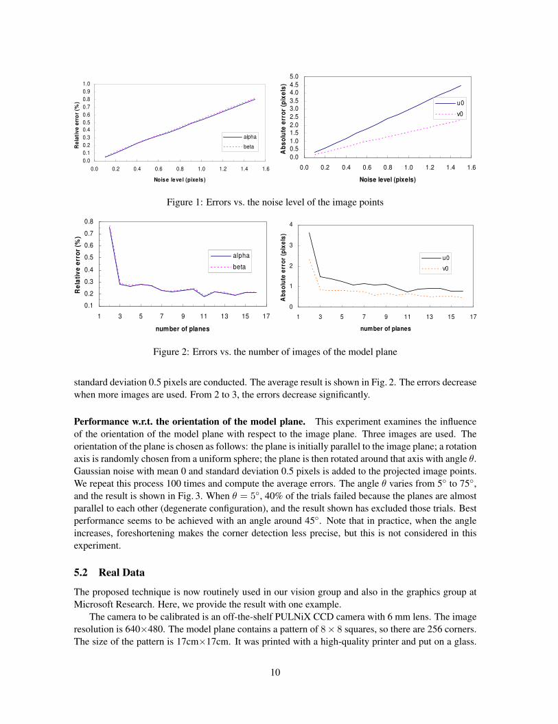
Performance w.r.t. the noise level. In this experiment, we use three planes with r1 = [20◦, 0, 0]T ,t1 = [−9,−12.5, 500]T , r2 = [0, 20◦, 0]T , t2 = [−9,−12.5, 510]T , r3 = 1√

5[−30◦,−30◦,−15◦]T ,

t3 = [−10.5,−12.5, 525]T . Gaussian noise with 0 mean and σ standard deviation is added to theprojected image points. The estimated camera parameters are then compared with the ground truth.We measure the relative error for α and β, and absolute error for u0 and v0. We vary the noise levelfrom 0.1 pixels to 1.5 pixels. For each noise level, we perform 100 independent trials, and the resultsshown are the average. As we can see from Fig. 1, errors increase linearly with the noise level. (Theerror for γ is not shown, but has the same property.) For σ = 0.5 (which is larger than the normalnoise in practical calibration), the errors in α and β are less than 0.3%, and the errors in u0 and v0 arearound 1 pixel. The error in u0 is larger than that in v0. The main reason is that there are less data inthe u direction than in the v direction, as we said before.

Performance w.r.t. the number of planes. This experiment investigates the performance with re-spect to the number of planes (more precisely, the number of images of the model plane). The orien-tation and position of the model plane for the first three images are the same as in the last subsection.From the fourth image, we first randomly choose a rotation axis in a uniform sphere, then apply arotation angle of 30◦. We vary the number of images from 2 to 16. For each number, 100 trialsof independent plane orientations (except for the first three) and independent noise with mean 0 and

9

0.0

0.1

0.2

0.3

0.4

0.5

0.6

0.7

0.8

0.9

1.0

0.0 0.2 0.4 0.6 0.8 1.0 1.2 1.4 1.6

Noise leve l (pixels )

Re

lati

ve

err

or

(%)

alpha

beta

0.0

0.5

1.0

1.5

2.0

2.5

3.0

3.5

4.0

4.5

5.0

0.0 0.2 0.4 0.6 0.8 1.0 1.2 1.4 1.6

Noise level (pixels)

Ab

so

lute

err

or

(pix

els

)

u0

v0

Figure 1: Errors vs. the noise level of the image points

0.1

0.2

0.3

0.4

0.5

0.6

0.7

0.8

1 3 5 7 9 11 13 15 17

number of planes

Re

lati

ve

err

or

(%)

alpha

beta

0

1

2

3

4

1 3 5 7 9 11 13 15 17

number of planes

Ab

so

lute

err

or

(pix

els

)

u0

v0

Figure 2: Errors vs. the number of images of the model plane

standard deviation 0.5 pixels are conducted. The average result is shown in Fig. 2. The errors decreasewhen more images are used. From 2 to 3, the errors decrease significantly.

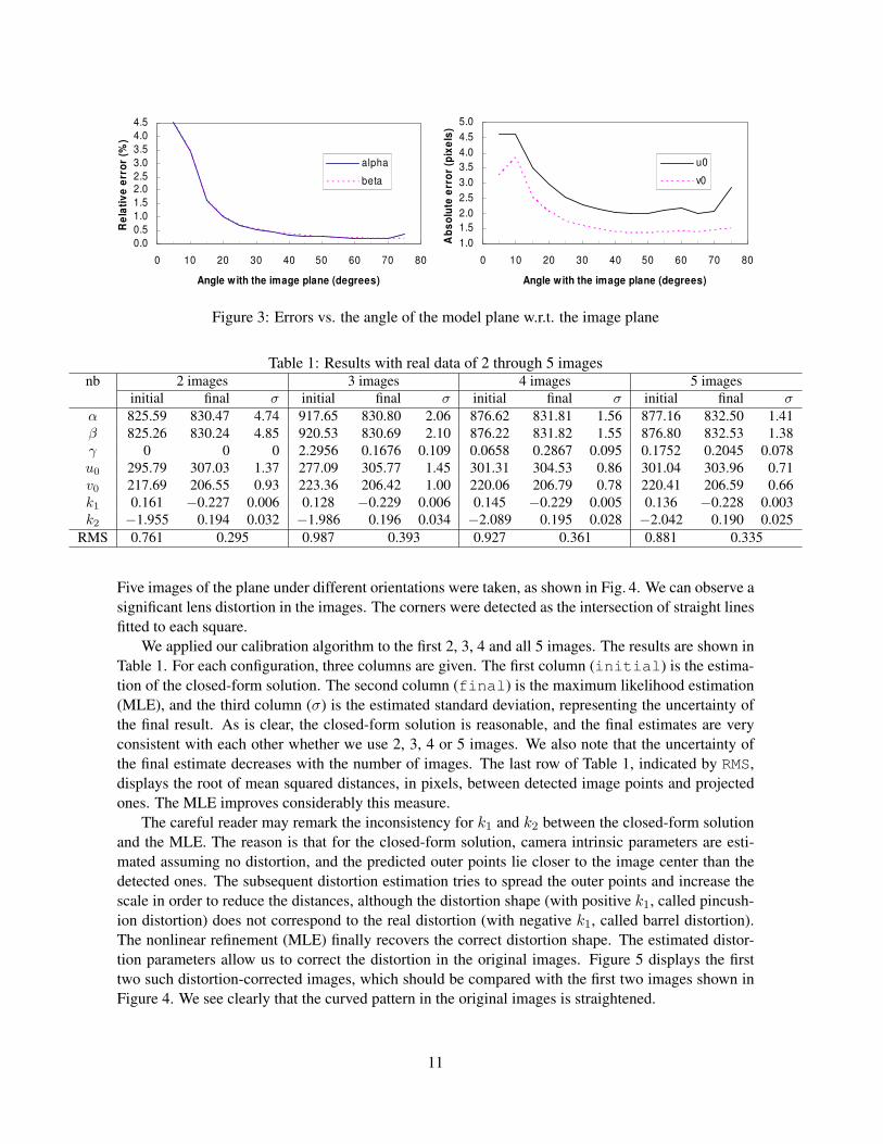
Performance w.r.t. the orientation of the model plane. This experiment examines the influenceof the orientation of the model plane with respect to the image plane. Three images are used. Theorientation of the plane is chosen as follows: the plane is initially parallel to the image plane; a rotationaxis is randomly chosen from a uniform sphere; the plane is then rotated around that axis with angle θ.Gaussian noise with mean 0 and standard deviation 0.5 pixels is added to the projected image points.We repeat this process 100 times and compute the average errors. The angle θ varies from 5◦ to 75◦,and the result is shown in Fig. 3. When θ = 5◦, 40% of the trials failed because the planes are almostparallel to each other (degenerate configuration), and the result shown has excluded those trials. Bestperformance seems to be achieved with an angle around 45◦. Note that in practice, when the angleincreases, foreshortening makes the corner detection less precise, but this is not considered in thisexperiment.

5.2 Real Data

The proposed technique is now routinely used in our vision group and also in the graphics group atMicrosoft Research. Here, we provide the result with one example.

The camera to be calibrated is an off-the-shelf PULNiX CCD camera with 6 mm lens. The imageresolution is 640×480. The model plane contains a pattern of 8× 8 squares, so there are 256 corners.The size of the pattern is 17cm×17cm. It was printed with a high-quality printer and put on a glass.

10

0.0

0.5

1.0

1.5

2.02.5

3.0

3.5

4.0

4.5

0 10 20 30 40 50 60 70 80

Angle with the image plane (degrees)

Re

lati

ve

err

or

(%)

alpha

beta

1.0

1.5

2.0

2.5

3.0

3.5

4.0

4.5

5.0

0 10 20 30 40 50 60 70 80

Angle with the image plane (degrees)

Ab

so

lute

err

or

(pix

els

)

u0

v0

Figure 3: Errors vs. the angle of the model plane w.r.t. the image plane

Table 1: Results with real data of 2 through 5 imagesnb 2 images 3 images 4 images 5 images

initial final σ initial final σ initial final σ initial final σα 825.59 830.47 4.74 917.65 830.80 2.06 876.62 831.81 1.56 877.16 832.50 1.41β 825.26 830.24 4.85 920.53 830.69 2.10 876.22 831.82 1.55 876.80 832.53 1.38γ 0 0 0 2.2956 0.1676 0.109 0.0658 0.2867 0.095 0.1752 0.2045 0.078u0 295.79 307.03 1.37 277.09 305.77 1.45 301.31 304.53 0.86 301.04 303.96 0.71v0 217.69 206.55 0.93 223.36 206.42 1.00 220.06 206.79 0.78 220.41 206.59 0.66k1 0.161 −0.227 0.006 0.128 −0.229 0.006 0.145 −0.229 0.005 0.136 −0.228 0.003k2 −1.955 0.194 0.032 −1.986 0.196 0.034 −2.089 0.195 0.028 −2.042 0.190 0.025

RMS 0.761 0.295 0.987 0.393 0.927 0.361 0.881 0.335

Five images of the plane under different orientations were taken, as shown in Fig. 4. We can observe asignificant lens distortion in the images. The corners were detected as the intersection of straight linesfitted to each square.

We applied our calibration algorithm to the first 2, 3, 4 and all 5 images. The results are shown inTable 1. For each configuration, three columns are given. The first column (initial) is the estima-tion of the closed-form solution. The second column (final) is the maximum likelihood estimation(MLE), and the third column (σ) is the estimated standard deviation, representing the uncertainty ofthe final result. As is clear, the closed-form solution is reasonable, and the final estimates are veryconsistent with each other whether we use 2, 3, 4 or 5 images. We also note that the uncertainty ofthe final estimate decreases with the number of images. The last row of Table 1, indicated by RMS,displays the root of mean squared distances, in pixels, between detected image points and projectedones. The MLE improves considerably this measure.

The careful reader may remark the inconsistency for k1 and k2 between the closed-form solutionand the MLE. The reason is that for the closed-form solution, camera intrinsic parameters are esti-mated assuming no distortion, and the predicted outer points lie closer to the image center than thedetected ones. The subsequent distortion estimation tries to spread the outer points and increase thescale in order to reduce the distances, although the distortion shape (with positive k1, called pincush-ion distortion) does not correspond to the real distortion (with negative k1, called barrel distortion).The nonlinear refinement (MLE) finally recovers the correct distortion shape. The estimated distor-tion parameters allow us to correct the distortion in the original images. Figure 5 displays the firsttwo such distortion-corrected images, which should be compared with the first two images shown inFigure 4. We see clearly that the curved pattern in the original images is straightened.

11

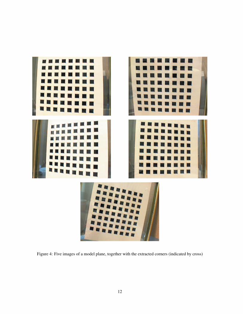
Figure 4: Five images of a model plane, together with the extracted corners (indicated by cross)

12

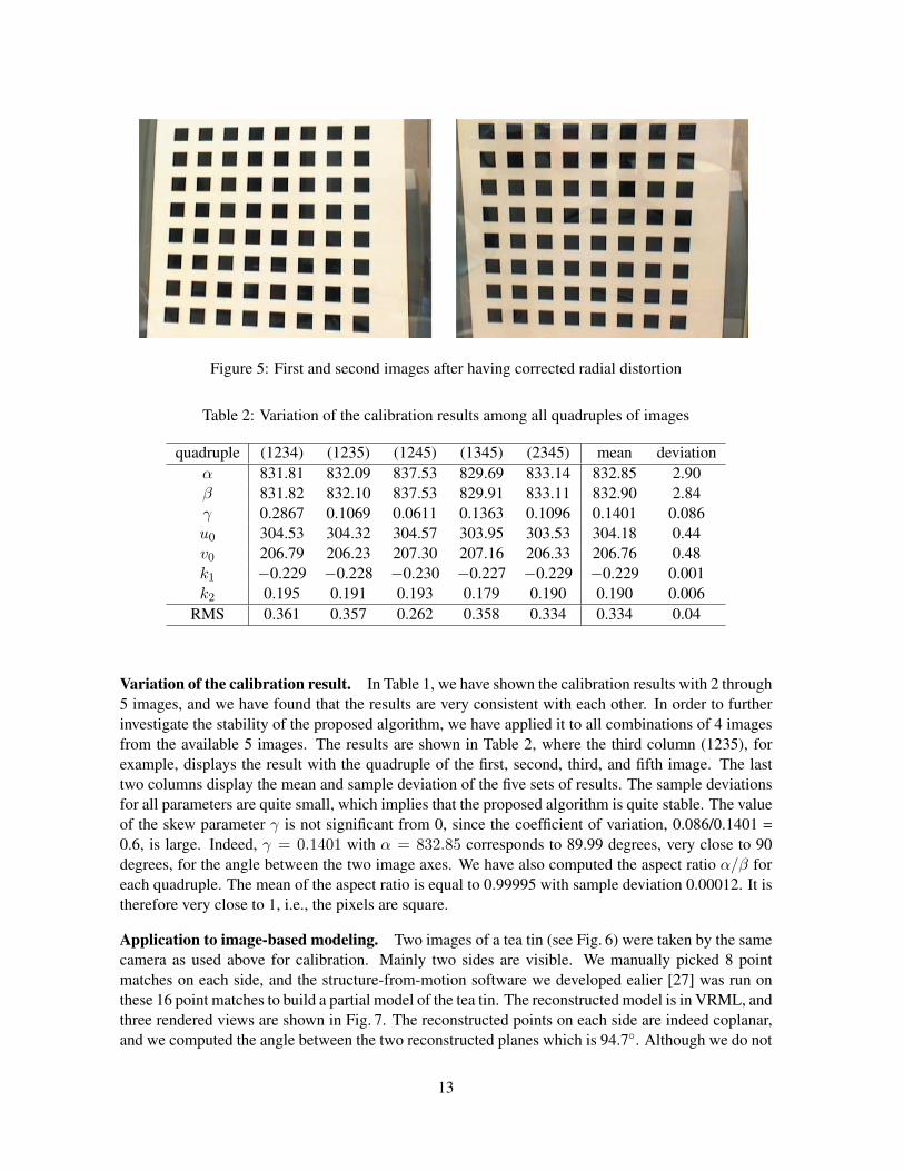
Figure 5: First and second images after having corrected radial distortion

Table 2: Variation of the calibration results among all quadruples of images

quadruple (1234) (1235) (1245) (1345) (2345) mean deviationα 831.81 832.09 837.53 829.69 833.14 832.85 2.90β 831.82 832.10 837.53 829.91 833.11 832.90 2.84γ 0.2867 0.1069 0.0611 0.1363 0.1096 0.1401 0.086u0 304.53 304.32 304.57 303.95 303.53 304.18 0.44v0 206.79 206.23 207.30 207.16 206.33 206.76 0.48k1 −0.229 −0.228 −0.230 −0.227 −0.229 −0.229 0.001k2 0.195 0.191 0.193 0.179 0.190 0.190 0.006

RMS 0.361 0.357 0.262 0.358 0.334 0.334 0.04

Variation of the calibration result. In Table 1, we have shown the calibration results with 2 through5 images, and we have found that the results are very consistent with each other. In order to furtherinvestigate the stability of the proposed algorithm, we have applied it to all combinations of 4 imagesfrom the available 5 images. The results are shown in Table 2, where the third column (1235), forexample, displays the result with the quadruple of the first, second, third, and fifth image. The lasttwo columns display the mean and sample deviation of the five sets of results. The sample deviationsfor all parameters are quite small, which implies that the proposed algorithm is quite stable. The valueof the skew parameter γ is not significant from 0, since the coefficient of variation, 0.086/0.1401 =0.6, is large. Indeed, γ = 0.1401 with α = 832.85 corresponds to 89.99 degrees, very close to 90degrees, for the angle between the two image axes. We have also computed the aspect ratio α/β foreach quadruple. The mean of the aspect ratio is equal to 0.99995 with sample deviation 0.00012. It istherefore very close to 1, i.e., the pixels are square.

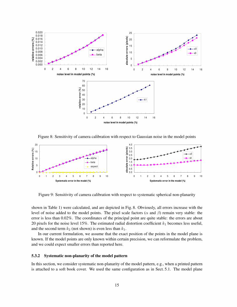
Application to image-based modeling. Two images of a tea tin (see Fig. 6) were taken by the samecamera as used above for calibration. Mainly two sides are visible. We manually picked 8 pointmatches on each side, and the structure-from-motion software we developed ealier [27] was run onthese 16 point matches to build a partial model of the tea tin. The reconstructed model is in VRML, andthree rendered views are shown in Fig. 7. The reconstructed points on each side are indeed coplanar,and we computed the angle between the two reconstructed planes which is 94.7◦. Although we do not

13

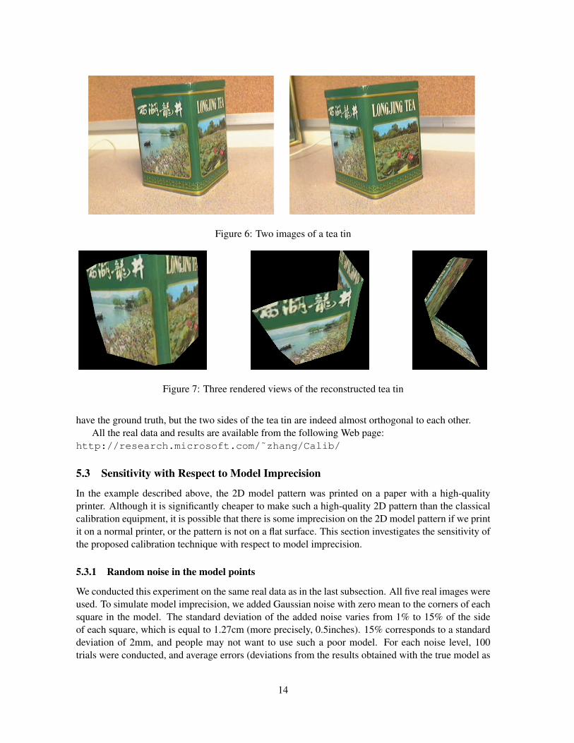
Figure 6: Two images of a tea tin

Figure 7: Three rendered views of the reconstructed tea tin

have the ground truth, but the two sides of the tea tin are indeed almost orthogonal to each other.All the real data and results are available from the following Web page:

http://research.microsoft.com/˜zhang/Calib/

5.3 Sensitivity with Respect to Model Imprecision

In the example described above, the 2D model pattern was printed on a paper with a high-qualityprinter. Although it is significantly cheaper to make such a high-quality 2D pattern than the classicalcalibration equipment, it is possible that there is some imprecision on the 2D model pattern if we printit on a normal printer, or the pattern is not on a flat surface. This section investigates the sensitivity ofthe proposed calibration technique with respect to model imprecision.

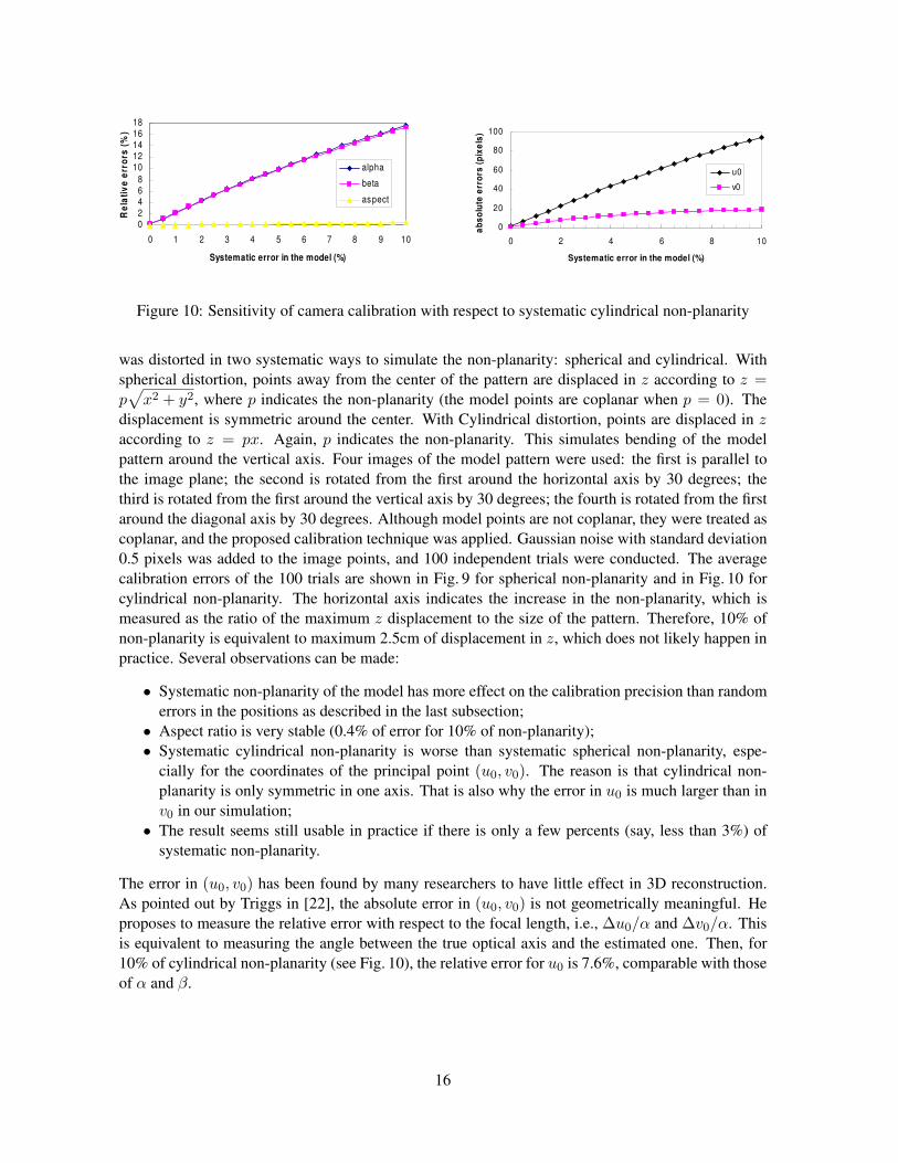
5.3.1 Random noise in the model points

We conducted this experiment on the same real data as in the last subsection. All five real images wereused. To simulate model imprecision, we added Gaussian noise with zero mean to the corners of eachsquare in the model. The standard deviation of the added noise varies from 1% to 15% of the sideof each square, which is equal to 1.27cm (more precisely, 0.5inches). 15% corresponds to a standarddeviation of 2mm, and people may not want to use such a poor model. For each noise level, 100trials were conducted, and average errors (deviations from the results obtained with the true model as

14

0.0000.0020.0040.0060.0080.0100.0120.0140.0160.0180.020

0 2 4 6 8 10 12 14 16

noise level in model points (%)

rela

tiv

e e

rro

rs (

%)

alpha

beta

0

5

10

15

20

25

0 2 4 6 8 10 12 14 16

noise level in model points (%)

ab

so

lute

err

ors

(p

ixe

ls)

u0

v0

0

10

20

30

40

50

60

70

0 2 4 6 8 10 12 14 16

noise level in model points (%)

rela

tiv

e e

rro

r (%

)

k1

Figure 8: Sensitivity of camera calibration with respect to Gaussian noise in the model points

0

5

10

15

20

0 1 2 3 4 5 6 7 8 9 10

Systematic error in the model (%)

Re

lati

ve

err

ors

(%

)

alpha

beta

aspect

0.0

0.5

1.0

1.5

2.0

2.5

3.0

3.5

4.0

0 1 2 3 4 5 6 7 8 9 10

Systematic error in the model (%)

ab

so

lute

err

or

(pix

els

)

u0

v0

Figure 9: Sensitivity of camera calibration with respect to systematic spherical non-planarity

shown in Table 1) were calculated, and are depicted in Fig. 8. Obviously, all errors increase with thelevel of noise added to the model points. The pixel scale factors (α and β) remain very stable: theerror is less than 0.02%. The coordinates of the principal point are quite stable: the errors are about20 pixels for the noise level 15%. The estimated radial distortion coefficient k1 becomes less useful,and the second term k2 (not shown) is even less than k1.

In our current formulation, we assume that the exact position of the points in the model plane isknown. If the model points are only known within certain precision, we can reformulate the problem,and we could expect smaller errors than reported here.

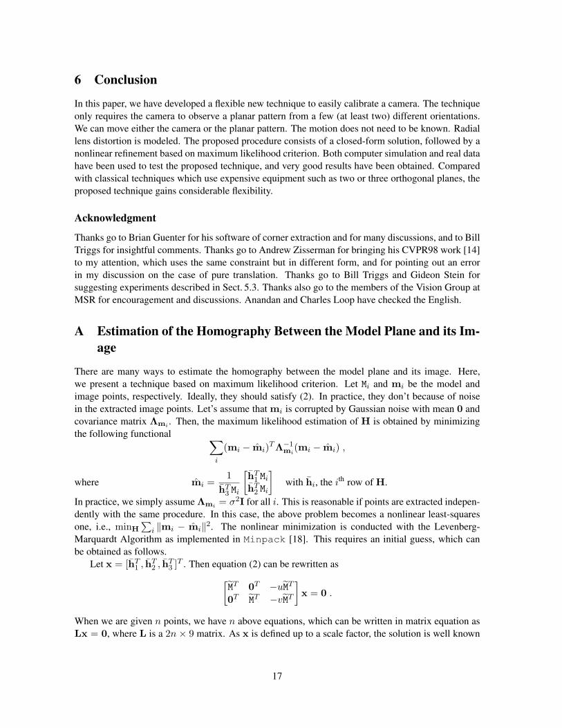
5.3.2 Systematic non-planarity of the model pattern

In this section, we consider systematic non-planarity of the model pattern, e.g., when a printed patternis attached to a soft book cover. We used the same configuration as in Sect. 5.1. The model plane

15

02468

1012141618

0 1 2 3 4 5 6 7 8 9 10

Systematic error in the model (%)

Re

lati

ve

err

ors

(%

)

alpha

beta

aspect

0

20

40

60

80

100

0 2 4 6 8 10

Systematic error in the model (%)

ab

so

lute

err

ors

(p

ixe

ls)

u0

v0

Figure 10: Sensitivity of camera calibration with respect to systematic cylindrical non-planarity

was distorted in two systematic ways to simulate the non-planarity: spherical and cylindrical. Withspherical distortion, points away from the center of the pattern are displaced in z according to z =p√

x2 + y2, where p indicates the non-planarity (the model points are coplanar when p = 0). Thedisplacement is symmetric around the center. With Cylindrical distortion, points are displaced in zaccording to z = px. Again, p indicates the non-planarity. This simulates bending of the modelpattern around the vertical axis. Four images of the model pattern were used: the first is parallel tothe image plane; the second is rotated from the first around the horizontal axis by 30 degrees; thethird is rotated from the first around the vertical axis by 30 degrees; the fourth is rotated from the firstaround the diagonal axis by 30 degrees. Although model points are not coplanar, they were treated ascoplanar, and the proposed calibration technique was applied. Gaussian noise with standard deviation0.5 pixels was added to the image points, and 100 independent trials were conducted. The averagecalibration errors of the 100 trials are shown in Fig. 9 for spherical non-planarity and in Fig. 10 forcylindrical non-planarity. The horizontal axis indicates the increase in the non-planarity, which ismeasured as the ratio of the maximum z displacement to the size of the pattern. Therefore, 10% ofnon-planarity is equivalent to maximum 2.5cm of displacement in z, which does not likely happen inpractice. Several observations can be made:

• Systematic non-planarity of the model has more effect on the calibration precision than randomerrors in the positions as described in the last subsection;

• Aspect ratio is very stable (0.4% of error for 10% of non-planarity);• Systematic cylindrical non-planarity is worse than systematic spherical non-planarity, espe-

cially for the coordinates of the principal point (u0, v0). The reason is that cylindrical non-planarity is only symmetric in one axis. That is also why the error in u0 is much larger than inv0 in our simulation;

• The result seems still usable in practice if there is only a few percents (say, less than 3%) ofsystematic non-planarity.

The error in (u0, v0) has been found by many researchers to have little effect in 3D reconstruction.As pointed out by Triggs in [22], the absolute error in (u0, v0) is not geometrically meaningful. Heproposes to measure the relative error with respect to the focal length, i.e., ∆u0/α and ∆v0/α. Thisis equivalent to measuring the angle between the true optical axis and the estimated one. Then, for10% of cylindrical non-planarity (see Fig. 10), the relative error for u0 is 7.6%, comparable with thoseof α and β.

16

6 Conclusion

In this paper, we have developed a flexible new technique to easily calibrate a camera. The techniqueonly requires the camera to observe a planar pattern from a few (at least two) different orientations.We can move either the camera or the planar pattern. The motion does not need to be known. Radiallens distortion is modeled. The proposed procedure consists of a closed-form solution, followed by anonlinear refinement based on maximum likelihood criterion. Both computer simulation and real datahave been used to test the proposed technique, and very good results have been obtained. Comparedwith classical techniques which use expensive equipment such as two or three orthogonal planes, theproposed technique gains considerable flexibility.

Acknowledgment

Thanks go to Brian Guenter for his software of corner extraction and for many discussions, and to BillTriggs for insightful comments. Thanks go to Andrew Zisserman for bringing his CVPR98 work [14]to my attention, which uses the same constraint but in different form, and for pointing out an errorin my discussion on the case of pure translation. Thanks go to Bill Triggs and Gideon Stein forsuggesting experiments described in Sect. 5.3. Thanks also go to the members of the Vision Group atMSR for encouragement and discussions. Anandan and Charles Loop have checked the English.

A Estimation of the Homography Between the Model Plane and its Im-age

There are many ways to estimate the homography between the model plane and its image. Here,we present a technique based on maximum likelihood criterion. Let Mi and mi be the model andimage points, respectively. Ideally, they should satisfy (2). In practice, they don’t because of noisein the extracted image points. Let’s assume that mi is corrupted by Gaussian noise with mean 0 andcovariance matrix Λmi . Then, the maximum likelihood estimation of H is obtained by minimizingthe following functional ∑

i

(mi − mi)TΛ−1mi

(mi − mi) ,

where mi =1

hT3 Mi

[hT

1 Mi

hT2 Mi

]with hi, the ith row of H.

In practice, we simply assume Λmi = σ2I for all i. This is reasonable if points are extracted indepen-dently with the same procedure. In this case, the above problem becomes a nonlinear least-squaresone, i.e., minH

∑i ‖mi − mi‖2. The nonlinear minimization is conducted with the Levenberg-

Marquardt Algorithm as implemented in Minpack [18]. This requires an initial guess, which canbe obtained as follows.

Let x = [hT1 , hT

2 , hT3 ]T . Then equation (2) can be rewritten as

[MT 0T −uMT

0T MT −vMT

]x = 0 .

When we are given n points, we have n above equations, which can be written in matrix equation asLx = 0, where L is a 2n× 9 matrix. As x is defined up to a scale factor, the solution is well known

17

to be the right singular vector of L associated with the smallest singular value (or equivalently, theeigenvector of LTL associated with the smallest eigenvalue).

In L, some elements are constant 1, some are in pixels, some are in world coordinates, and someare multiplication of both. This makes L poorly conditioned numerically. Much better results can beobtained by performing a simple data normalization, such as the one proposed in [12], prior to runningthe above procedure.

B Extraction of the Intrinsic Parameters from Matrix B

Matrix B, as described in Sect. 3.1, is estimated up to a scale factor, i.e., , B = λA−TA with λ anarbitrary scale. Without difficulty†, we can uniquely extract the intrinsic parameters from matrix B.

v0 = (B12B13 −B11B23)/(B11B22 −B212)

λ = B33 − [B213 + v0(B12B13 −B11B23)]/B11

α =√

λ/B11

β =√

λB11/(B11B22 −B212)

γ = −B12α2β/λ

u0 = γv0/β −B13α2/λ .

C Approximating a 3× 3 matrix by a Rotation Matrix

The problem considered in this section is to solve the best rotation matrix R to approximate a given3× 3 matrix Q. Here, “best” is in the sense of the smallest Frobenius norm of the difference R−Q.That is, we are solving the following problem:

minR‖R−Q‖2

F subject to RTR = I . (15)

Since

‖R−Q‖2F = trace((R−Q)T (R−Q))

= 3 + trace(QTQ)− 2trace(RTQ) ,

problem (15) is equivalent to the one of maximizing trace(RTQ).Let the singular value decomposition of Q be USVT , where S = diag (σ1, σ2, σ3). If we define

an orthogonal matrix Z by Z = VTRTU, then

trace(RTQ) = trace(RTUSVT ) = trace(VTRTUS)

= trace(ZS) =3∑

i=1

ziiσi ≤3∑

i=1

σi .

It is clear that the maximum is achieved by setting R = UVT because then Z = I. This gives thesolution to (15).

An excellent reference on matrix computations is the one by Golub and van Loan [10].†A typo was reported in formula u0 by Jiyong Ma [mailto:jiyong@cslr.Colorado.EDU] via an email on April 18, 2002.

18

D Camera Calibration Under Known Pure Translation

As said in Sect. 4, if the model plane undergoes a pure translation, the technique proposed in thispaper will not work. However, camera calibration is possible if the translation is known like the setupin Tsai’s technique [23]. From (2), we have t = αA−1h3, where α = 1/‖A−1h1‖. The translationbetween two positions i and j is then given by

t(ij) = t(i) − t(j) = A−1(α(i)h(i)3 − α(j)h(j)

3 ) .

(Note that although both H(i) and H(j) are estimated up to their own scale factors, they can be rescaledup to a single common scale factor using the fact that it is a pure translation.) If only the translationdirection is known, we get two constraints on A. If we know additionally the translation magnitude,then we have another constraint on A. Full calibration is then possible from two planes.

19

References

[1] S. Bougnoux. From projective to euclidean space under any practical situation, a criticism ofself-calibration. In Proceedings of the 6th International Conference on Computer Vision, pages790–796, Jan. 1998.

[2] D. C. Brown. Close-range camera calibration. Photogrammetric Engineering, 37(8):855–866,1971.

[3] B. Caprile and V. Torre. Using Vanishing Points for Camera Calibration. The InternationalJournal of Computer Vision, 4(2):127–140, Mar. 1990.

[4] W. Faig. Calibration of close-range photogrammetry systems: Mathematical formulation. Pho-togrammetric Engineering and Remote Sensing, 41(12):1479–1486, 1975.

[5] O. Faugeras. Three-Dimensional Computer Vision: a Geometric Viewpoint. MIT Press, 1993.

[6] O. Faugeras, T. Luong, and S. Maybank. Camera self-calibration: theory and experiments. InG. Sandini, editor, Proc 2nd ECCV, volume 588 of Lecture Notes in Computer Science, pages321–334, Santa Margherita Ligure, Italy, May 1992. Springer-Verlag.

[7] O. Faugeras and G. Toscani. The calibration problem for stereo. In Proceedings of the IEEEConference on Computer Vision and Pattern Recognition, pages 15–20, Miami Beach, FL, June1986. IEEE.

[8] S. Ganapathy. Decomposition of transformation matrices for robot vision. Pattern RecognitionLetters, 2:401–412, Dec. 1984.

[9] D. Gennery. Stereo-camera calibration. In Proceedings of the 10th Image Understanding Work-shop, pages 101–108, 1979.

[10] G. Golub and C. van Loan. Matrix Computations. The John Hopkins University Press, Balti-more, Maryland, 3 edition, 1996.

[11] R. Hartley. Self-calibration from multiple views with a rotating camera. In J.-O. Eklundh, editor,Proceedings of the 3rd European Conference on Computer Vision, volume 800-801 of LectureNotes in Computer Science, pages 471–478, Stockholm, Sweden, May 1994. Springer-Verlag.

[12] R. Hartley. In defence of the 8-point algorithm. In Proceedings of the 5th International Confer-ence on Computer Vision, pages 1064–1070, Boston, MA, June 1995. IEEE Computer SocietyPress.

[13] R. I. Hartley. An algorithm for self calibration from several views. In Proceedings of the IEEEConference on Computer Vision and Pattern Recognition, pages 908–912, Seattle, WA, June1994. IEEE.

[14] D. Liebowitz and A. Zisserman. Metric rectification for perspective images of planes. In Pro-ceedings of the IEEE Conference on Computer Vision and Pattern Recognition, pages 482–488,Santa Barbara, California, June 1998. IEEE Computer Society.

20

[15] Q.-T. Luong. Matrice Fondamentale et Calibration Visuelle sur l’Environnement-Vers une plusgrande autonomie des systemes robotiques. PhD thesis, Universite de Paris-Sud, Centre d’Orsay,Dec. 1992.

[16] Q.-T. Luong and O. Faugeras. Self-calibration of a moving camera from point correspondencesand fundamental matrices. The International Journal of Computer Vision, 22(3):261–289, 1997.

[17] S. J. Maybank and O. D. Faugeras. A theory of self-calibration of a moving camera. TheInternational Journal of Computer Vision, 8(2):123–152, Aug. 1992.

[18] J. More. The levenberg-marquardt algorithm, implementation and theory. In G. A. Watson,editor, Numerical Analysis, Lecture Notes in Mathematics 630. Springer-Verlag, 1977.

[19] I. Shimizu, Z. Zhang, S. Akamatsu, and K. Deguchi. Head pose determination from one imageusing a generic model. In Proceedings of the IEEE Third International Conference on AutomaticFace and Gesture Recognition, pages 100–105, Nara, Japan, Apr. 1998.

[20] C. C. Slama, editor. Manual of Photogrammetry. American Society of Photogrammetry, fourthedition, 1980.

[21] G. Stein. Accurate internal camera calibration using rotation, with analysis of sources of er-ror. In Proc. Fifth International Conference on Computer Vision, pages 230–236, Cambridge,Massachusetts, June 1995.

[22] B. Triggs. Autocalibration from planar scenes. In Proceedings of the 5th European Conferenceon Computer Vision, pages 89–105, Freiburg, Germany, June 1998.

[23] R. Y. Tsai. A versatile camera calibration technique for high-accuracy 3D machine visionmetrology using off-the-shelf tv cameras and lenses. IEEE Journal of Robotics and Automa-tion, 3(4):323–344, Aug. 1987.

[24] G. Wei and S. Ma. A complete two-plane camera calibration method and experimental compar-isons. In Proc. Fourth International Conference on Computer Vision, pages 439–446, Berlin,May 1993.

[25] G. Wei and S. Ma. Implicit and explicit camera calibration: Theory and experiments. IEEETransactions on Pattern Analysis and Machine Intelligence, 16(5):469–480, 1994.

[26] J. Weng, P. Cohen, and M. Herniou. Camera calibration with distortion models and accuracyevaluation. IEEE Transactions on Pattern Analysis and Machine Intelligence, 14(10):965–980,Oct. 1992.

[27] Z. Zhang. Motion and structure from two perspective views: From essential parametersto euclidean motion via fundamental matrix. Journal of the Optical Society of America A,14(11):2938–2950, 1997.

21