A fistful of Euros: Does One-Euro-Job participation lead means-testedbenefit recipients into regular jobs and out of unemployment benefit II

receipt?

Katrin HohmeyerInstitute for Employment Research

Joachim WolffInstitute for Employment Research

(January 2008)

LASER Discussion Papers - Paper No. 13

(edited by A. Abele-Brehm, R.T. Riphahn, K. Moser and C. Schnabel)

Correspondence to:

Katrin Hohmeyer, Regensburger Straße 104 , 90478 Nuremberg, Germany, Email:Katrin.Hohmeyer@iab.de.

Abstract

In 2005 a major reform of the German means-tested unemployment benefit system came into force.The reform aimed at activating benefit recipients, e.g., by a workfare programme, the so-calledOne-Euro-Job. This programme was implemented at a large scale. Participants receive theirmeans-tested benefit and a small compensation of usually one to 1.5 € per hour worked. Participationtypically lasts six months or less. We investigate the impact of One-Euro-Jobs for participants whoentered the programme at the start of the year 2005. We apply propensity score matching to estimatethe treatment effects on the outcomes regular employment, neither being registered as unemployed noras job-seeker and no unemployment benefit II receipt. We observe these outcomes for about two yearsafter programme start. The locking-in effects are small. Moreover, 20 months after programme there isa significant but small positive impact on the employment rate of female but not male participants.During the first two years after programme start, participation does not contribute to avoidingunemployment benefit II receipt. Our results imply that there is some effect heterogeneity:Participation reduces the employment rate of participants younger than 25 years, but raises it for someolder participant groups. It is ineffective for participants who were recently employed, while it iseffective for participants who lost their last contributory job between 1992 and 2000.

Copyright statement

Please do not quote without permission from the authors. Only the final version that will be acceptedfor publication should be cited. This document has been posted for the purpose of discussion and rapiddissemination of preliminary research results.

A fistful of Euros: Does One-Euro-Job participation lead means-tested benefit

recipients into regular jobs and out of unemployment benefit II receipt?

Katrin Hohmeyer and Joachim Wolff

CONTENTS

1. Introduction ..........................................................................................................................1

2. Institutional framework and target groups of One-Euro-Jobs ........................................3

3. Literature review ..................................................................................................................4

4. Theoretical background and hypotheses............................................................................7

5. Methods and data ...............................................................................................................10 5.1 Methods .............................................................................................................................10 5.2 Data....................................................................................................................................12

6. Results: Average treatment effects on the treated of One-Euro-Jobs ...........................14 6.1 Implementation.................................................................................................................14 6.2 Match quality, sensitivity analysis ..................................................................................15 6.3 Overall effects ...................................................................................................................17 6.4 Effects by age ....................................................................................................................19 6.5 Effects by nationality........................................................................................................21 6.6 Effects by occupational qualification..............................................................................21 6.7 Effects by regional unemployment rate..........................................................................22 6.8 Effects by time since last employment ............................................................................22

7. Summary and conclusions .................................................................................................23

References ...............................................................................................................................26

Tables and figures...................................................................................................................29

1

1. Introduction Due to high and persistent unemployment reforms of German labour market policy in the last years concentrated to a large extent on activation policies for unemployed persons.1 One of the reforms was implemented with the introduction of the Social Code II. A new means-tested benefit, the unemployment benefit II (UB II), was introduced at the start of the year 2005. It replaced the two former means-tested benefits, unemployment assistance and social benefit, for employable persons in needy households. The Social Code II in contrast to the former system emphasises activation policies. One of these policies is a workfare programme, which was implemented at a large scale: The work opportunity programme in which participants receive their unemployment benefit II and additionally one to two Euros per hour worked - the so called One-Euro-Job.2 In this paper we evaluate whether participation in the One-Euro-Job scheme improves the labour market performance of participants.

One-Euro-Jobs are subordinate to regular employment, vocational training and other active labour market programmes. The jobs have to be of public interest and additional in the sense that they would not be carried out without the subsidy. In so far they are similar to traditional job creation schemes. Yet, while in the latter type of programme participants receive a wage, participants in One-Euro-Jobs receive their UB II and as already mentioned additionally a small compensation for their working-time. The basic goal of One-Euro-Jobs is to activate those UB II recipients who have particular difficulties in finding a job. Nevertheless, UB II agencies can rely on the programme as a work-test. After the introduction of the Social Code II the programme became the most important active labour market policy in Germany in terms of the number of persons entering the programme. More than 600,000 persons were registered as starting the programme in the year 2005 and even more than 700,000 in the year 2006. Compared to the stock of unemployed recipients of UB II of roughly two and a half million in those years the size of the inflow is very high.

To our knowledge there is no study on the impact of participation in the One-Euro-Job programme on the labour market performance of participants. Quantifying such effects is particularly important from a policy point of view, since the programme attempts to improve the employability of people whose job-finding perspectives are among the worst. It is also of much interest from a more general point of view, as we can determine how workfare influences different types of participants: Given the large scale of the programme, we can estimate treatment effects on the treated separately for many

1 A comprehensive description of recent institutional changes of German labour market policy can be

found in Jacobi and Kluve (2007). These reforms are well known in Germany as the Hartz reforms, as many of them were proposed by a commission that was led by Peter Hartz, head of the personnel executive committee of Volkswagen.

2 Similar measures existed under the old social assistance regime: the Help Towards Work (Hilfe zur Arbeit) programme created work opportunities to integrate social assistance recipients into work and in order to test their willingness to work. Municipalities organised the programme independently and without any central coordination, such that their implementation at the local level came in a wide variety of forms (Voges et al. 2001). An evaluation of the effectiveness of these programmes was not carried out, due to the lack of micro data. For a description of the Help Towards Work programme see for example Voges et al. (2001).

2

different groups of participants who entered the programme over a very short period of time.

In contrast to most evaluation studies that estimate programme effects with administrative data, we can incorporate considerable information on the household of programme participants and control individuals. The introduction of the Social Code II also implemented a new data collection system which makes unemployment benefit II agencies collect information on all members of needy households. In turn any member of an unemployment benefit II recipient household can be tracked over time and the administrative data of partners or other household members on employment, unemployment, active labour market programme participation, benefit receipt from other administrative data sources can be retrieved for our analysis. With this data set-up many research questions in the context of poor households can be addressed using the entire population of households with means-tested benefit receipt and not just small samples.

Our study estimates the effect of programme participation using matching methods. The effects are estimated for the entire inflow into the One-Euro-Job programme during the months February to April 2005. We only regard programme participants if they were unemployed on 31st January 2005 and received UB II at that time. The potential control group members stem from a 20 percent random sample of needy persons in the unemployment stock at the end of January 2005. Of course we excluded all people from the unemployment stock, who started a One-Euro-Job from February to April 2005. However, controls may enter this programme at later points in time. Hence, we estimate the effect of joining the programme in this time period.

We are concerned with effects of programme participation on the regular employment rate, on whether the participants are neither registered as unemployed nor job-seeking and on the rate of no UB II receipt. The effects are generally estimated separately for men and women in East and in West Germany, given the different labour market situation of the two German regions. However, we also deal with effect heterogeneity according to age, nationality/migration status, occupational qualification, the regional unemployment rate, and time since last regular employment. This should first of all show for which groups the programme is most effective in its current set-up. It should also give some insights on why and when the policy achieves or fails to achieve (some of) its goals: E.g., the programme may improve employability of the participants, though not sufficiently to lead to an immediate success in terms of an increased employment rate. However, in a low unemployment region the improvement of employability is more likely to also affect the regular employment rate than in a region with high unemployment.

The paper is structured as follows: Section two describes the institutional set-up of the new unemployment benefit II and of the related One-Euro-Job programme. In section three, we provide a short literature review on the effects of workfare programmes and public employment schemes. Section four discusses a theoretical background for our analysis together with some key hypotheses of our study. The methods and data are described in section five. We discuss the results of our analysis in section six and briefly summarize and conclude in the final section seven.

3

2. Institutional framework and target groups of One-Euro-Jobs With the introduction of the Social Code II at the start of the year 2005 major reforms of the German unemployment compensation system came into force (the so called “Hartz IV”-reforms). A new means-tested benefit system was introduced: The unemployment benefit II (UB II) replaced the former means-test unemployment assistance (UA) and social assistance (SA) for needy employable people.3,4 The reform did not generally cut benefit levels for needy households.5 The central idea behind introducing the Social Code II was to activate needy people, so that more of them are integrated into the labour market and their benefit dependency should be reduced. This is of particular importance for people who without the reform would have received SA benefit as well as for people who would have been partners or other household members of a UA benefit recipient. Without the reform such people would not necessarily have been in contact with labour agencies, registered as unemployed or as job-seekers nor would they have qualified for many types of active labour market policies. Due to the reform this has changed and each employable member of a needy household is supposed to contribute to reducing the dependency on the means-tested benefit.

On the one hand, the Social Code II demands efforts of unemployed persons with regard to job search and other activities to improve their chances of finding a job. Integration contracts and benefit sanctions for those who do not comply to the rules are instruments to raise such efforts. On the other hand, the reform provides more possibilities of assisting unemployed persons towards employment take-up and in particular led to more intensive active labour market policies.

One option of promoting and challenging unemployed persons is public employment such as work opportunities that have their legal basis in the Social Code II. Two types of work opportunities exist: (a) Work opportunities with wage (“Arbeitsgelegenheiten in der Entgeltvariante”) and (b) work opportunities with an allowance to unemployment benefit II for additional expenses (“Arbeitsgelegenheiten in der Mehraufwandsvariante” or “One-Euro-Jobs”). More than 95% of the programme starts of work opportunities are One-Euro-Jobs, so that we regard this latter programme.

3 The old unemployment insurance (UI) benefit was labelled as unemployment benefit I. It is

earnings-related with a replacement rate of 67 percent for a parent and 60 percent for childless people. The UI benefit in contrast to UB II is time-limited, where the length of receipt increases with the time a recipient has contributed to unemployment insurance within a period of seven years prior to the benefit claim. The maximum duration of UI receipt though depends on age and was one year for those aged younger than 45 in the year 2005. It increased for older age groups and those older than 56 years could even receive their UI benefit up to 32 months. The maximum durations of those older than 44 years though were considerably reduced in the year 2006.

4 People who are aged between 15 and 64 and can work under the usual conditions of the labour market for at least three hours a day are regarded as employable. Only due to an illness or disability, it is possible not to fulfil this criterion (Article 8 Social Code II).

5 Blos and Rudolph (2005) showed in a simulation study based on micro data from an income and consumption survey how the benefit levels of former social benefit recipients and former unemployment assistance recipients were affected by the benefit reform. It did not much affect benefit levels of households of former social benefit recipients. However, about 17 percent of former unemployment assistance recipients no longer qualified for the new means-tested benefit. Of those former unemployment assistance households, which qualified for UB II, about 50 percent faced benefit reductions and 50 percent a benefit increase.

4

There are various goals of the One-Euro-Job programme (Federal Employment Agency 2005). They should raise the employability of long-term unemployed persons and enhance their chances of finding regular employment. Furthermore, they aim at the social integration of needy unemployed persons by providing them with a task and a daily routine. Moreover, they can be seen as a contribution to the provision of public goods by the needy people who have to work for their UB II receipt. Finally, One-Euro-Jobs are also a means of testing an unemployed person’s willingness to work.

The tasks carried out in One-Euro-Jobs have to be of public utility and additional in the sense that they would not be completed without the subsidy. In the year 2005 most One-Euro-Job participations lasted up to six months (Hohmeyer et al. 2006). Additional expenses in One-Euro-Jobs average 1.25 € per hour worked (Wolff/Hohmeyer 2006). Regarding the average working time of One-Euro-Jobs of nearly 30 hours per week this adds up to about 145 € per month additional to UB II. UB II consists of a base benefit currently at 347 € per month for a single person6 costs of accommodation and heating and an additional benefit for those who received within the last two years unemployment insurance (UI) benefit.7

One-Euro-Jobs are designed for employable needy persons aged between 15 and 64 years. They are subordinate to regular employment, vocational training and other active labour market programmes. Thus, they are a measure of last resort and persons with specific difficulties to find employment should be more likely to participate in One-Euro-Jobs than those with better chances of finding a job. This at least partly conflicts with the idea that the programme should serve as a work-test. Such a work-test is more likely to be effective for people with good job finding perspectives. Hence, it is not surprising that recent research describing the structure of participants (inflow) shows that One-Euro-Jobs are not targeted on specific groups of unemployed people, who are hard to place (Heinemann et al. 2006, Hohmeyer et al. 2006, Wolff/Hohmeyer 2006). This may either be due to cream skimming or to the use of One-Euro-Jobs as a work test.

3. Literature review As work opportunities have just been introduced in January 2005, no evaluation results are available for this specific programme in Germany. Nevertheless, it is worth discussing the lessons learned from the evaluation literature on similar programmes both in Germany and in other countries. Of course such evaluation results cannot be just transferred to our context as they have emerged for programmes that differed from work

6 When the new system was introduced in the year 2005 this base benefit of ‘unemployment benefit

II’ was lower 345 Euro for a lone adult or lone parent in West Germany and Berlin and 331 Euro in the five federal states in East Germany. It was raised to the Western level for UB II recipients in the East German federal states in July 2006.

7 The additional benefit is related to the difference between the sum of the former UI and housing benefit receipt and the UB II benefit level. It amounts to two thirds of this difference in the first year after running out of UI receipt. However, there is an upper cap for the additional benefit of 160 € for singles and 320 € for partners. For each child that lives in the needy household of a person who is eligible for the additional benefit, the upper cap is raised by 60 €. In the second year after exhausting UI benefit receipt the additional benefit is cut by 50 percent.

5

opportunities in several aspects, have taken place in a different context and for different groups of participants.

The German work opportunity programme resembles first, public employment programmes for unemployment benefit recipients and second, workfare programmes for social benefit recipients. One-Euro-Jobs are similar to both of them, as the two types of programmes are supposed to create jobs of public interest that do not compete with existing private sector jobs. But while public employment programmes mainly aim at integrating participants into the labour market, workfare programmes also imply that participants reciprocate for the benefit receipt. In turn for the benefit receipt which is financed by the society participants contribute to the provision of public goods.

Evidence on Germany

a) public employment programmes

Job creation schemes have already been introduced in Germany in 1969 with the job promotion law (“Arbeitsförderungsgesetz”). In 2000 job creation schemes were one of the most widely-used active labour market programmes. Just like One-Euro-Jobs job creation schemes have to be of public use and additional. In contrast to participants of One-Euro-Jobs persons working in a job creation scheme receive a wage. And of course the group of participants is different: Till the end of 2004 only those persons who received UI or UA benefit were eligible to participate in job creation schemes.

Recently, the effectiveness of the scheme for the participants has been studied intensively. Applying a statistical matching approach Caliendo, Hujer and Thomsen investigated in several non-experimental studies the impact of German job creation schemes on the labour market performance of participants who started their job creation scheme at the beginning of the year 2000 (Caliendo 2006; Caliendo et al. 2005a, b).8 Positive effects of public employment programmes on the regular employment rate of participants can only be found for a few specific groups and only nearly three years after programme start (Caliendo et al. 2005a, b). For participants taken together and in the short run public employment programmes have a negative or zero impact on employment chances. Participation raises the employment rate of long-term unemployed people, highly qualified men with above average labour market prospects and West German women, in particularly those who are older than 50 years or long-term unemployed (Caliendo 2006). This beneficial effect though only emerges at about nearly three years after programme start. Participation is associated with high locking-in effects given that it lasts about one year.

b) “Help Towards Work“ (Hilfe zur Arbeit) for recipients of social benefits

Despite the high number of participants in the German „Help Towards Work“ programme no evaluation studies on its labour market impacts exist. The reason for this is that the programme was placed to the local authorities’ responsibility and therefore large regional differences existed. Some regional studies in the form of integration rates and cost benefit analyses exist (e.g., Böckmann-Schewe/Röhrig 1997; Kempken/Trube

8 The authors estimated the treatment effects on the treated with matching estimators.

6

1997; Trube 1994). But without comparing integration rates of participants to those of a suitable comparison group, the studies are not regarding the effectiveness of the programme.

International Evidence The international studies can also be divided into the two fields of employment programmes for unemployment insurance benefit recipients who are rather close to the labour market and workfare programmes for social welfare recipients.

a) public employment programmes

Gerfin and Lechner (2001) investigate the impacts of various active labour market schemes in Switzerland on the employment probability of participants. These employment programmes (partly) have to create jobs that are additional like One-Euro-Jobs. The results of the study suggest that participation decreases the employment probability during the first 15 months after programme start. Only for women who start a programme in the public sector their employment rate after participation is higher than after non-participation. Moreover, the authors find positive impacts on the employment rate of participants for wage subsidies for jobs that are not required to be additional. Thus, they conclude that an important factor for the success of a programme is that the subsidised jobs are similar to regular jobs.

Calmfors et al. (2002) come to the same conclusion as Gerfin and Lechner (2001) in their overview of Swedish evaluation studies regarding different outcome variables: the effect of an employment programme increases if the job is closer to the labour market. Programmes like “relief work” and “work experience” are similar to One-Euro-Jobs in the respect that they are not similar to jobs in the regular labour market. They have either negative or zero effects on the labour market performance of participants.

b) workfare programmes

By “Workfare” we understand public employment programmes for recipients of social benefits. Following Lodemel (2000, 2005) workfare programmes show three constituting elements:

• Participation is compulsory. Benefits can be cut if needy persons refuse to participate. This means unemployment is also regarded as a lack of motivation.

• The programme is primarily about work. Qualification can be but is not necessarily content of the programme.

• Workfare is targeted on social benefit recipients. Benefit recipients are supposed to work for or instead of receiving benefits.

Following this definition One-Euro-Jobs are a workfare programme. Therefore, some lessons can be learned from the evaluation literature on workfare programmes in other countries.

Gueron and Pauly (1991) find positive effects of temporary workfare-programmes in the United States: future income of participants increases compared to non-participants.

7

Lissenburgh (2001) identifies for Great Britain that the New Deal for Long-Term Unemployed has a positive impact on labour market chances of participants. However, the considered programmes are mainly wage subsidies. Thus, comparability with One-Euro-Jobs is restricted.

Also in Denmark positive impacts of workfare programmes on labour market performance of participants can be found: Bolvig et al. (2003) find that workfare reduces the duration of benefit receipt mainly for persons with various placement barriers und persons under the age of 25. Locking-in effects are stronger for women than for men. Though participation in the considered programmes improves the chances of leaving welfare receipt, the duration of the subsequent employment cannot be increased.

Ochel (2004) resumes evaluation studies from various countries and concludes that subsidised employment is more effective than employment in programmes that are very distant to the labour market. Locking-in effects occur for employment programmes in the public sector.

To sum up, public employment schemes seem to be effective only for specific groups of participants. However, the results of the discussed evaluation studies do not allow us to draw already conclusions on the impact of participation in One-Euro-Jobs.

On the one hand a positive impact of One-Euro-Jobs on the labour market performance of participants can be expected, if we consider that job creation schemes enhanced labour market prospects for long-term unemployed participants, a group who can be regarded as similar to unemployment benefit II recipients (Caliendo 2006). On the other hand an adverse impact may be expected since One-Euro-Jobs have to be additional and of public interest (see results from Gerfin/Lechner 2001; Ochel 2004). Therefore the impacts of One-Euro-Jobs besides a short-term labour market relief are not known ex-ante. Considering the quantitative importance of One-Euro-Jobs and the persistent high rates of unemployment more knowledge about the impact of One-Euro-Jobs on individual employment chances is desirable.

4. Theoretical background and hypotheses Active labour market policies (ALMPs) affect the labour market through a number of channels: e.g. by changing the matching efficiency between labour demand and labour supply, altering labour demand and supply at a given wage rate or by altering the wage-setting process (Calmfors 1994). In this paper we are concerned with the micro-effects of One-Euro-Jobs on participants. The participation in ALMP may influence the participants' labour market performance in various ways.

ALMPs may raise the effectiveness of job search of participants: Calmfors (1994) as well as Hagen and Steiner (2000) mention some reasons for this: First of all, qualifications of the job searchers adjust to requirements of job vacancies. Adjustment becomes necessary as according to human capital theory unemployment leads to loss of human capital and due to structural shifts in qualification requirements. In this context One-Euro-Jobs could be beneficial, since participants may be trained on the job. Moreover, by participating in the programme long-term non-employed people could compensate for a loss of very basic skills, e.g., if they are no longer used to regular work-schedules. This might increase the participants' probability of getting a job offer.

8

Second, ALMP participation could also achieve a rise in the arrival rate of job offers, because it signals employers the participant's the willingness to work. Finally, ALMPs could raise the search effort of participants: One-Euro-Jobs may reduce the value of benefit receipt due to a loss of leisure and because of making it harder to achieve earnings in the shadow economy.

Besides these desired effects, adverse effects can occur. First, locking-in effects can arise, that reduce efforts made by unemployed persons to search for employment. While participating in One-Euro-Jobs, a person's search efforts decrease, e.g., because participation reduces the time available for job search. Furthermore participation can reduce the motivation to look for employment because participants derive some utility from programme participation, e.g., due to carrying out a useful task instead of being without employment. Job search efforts can already decline before participation started if the unemployed person knows about his participation in advance (“Ashenfelter’s Dip”).

Even if the One-Euro-Job participation increases search efforts of the participants and they more quickly find regular employment than others, there still could be some adverse effects. Assume that the programme works partly through making benefit receipt more inconvenient for the participants. Moreover, assume that participants are aware of the fact that without participating in the programme, they would have faced benefit sanctions. Then the treatment could lead to faster job finding through lower reservation wages, such that participants tend to accept lower paid jobs than non-participants. In that case even if the regular employment rate of participants is raised, the likelihood that the households of the treated individuals are no longer needy may be adversely affected.

Moreover employers possibly do not regard active labour market programmes as equivalent to regular employment or other forms of qualification (stigma effect). This is likely to be the case if a programme like work opportunities is supposed to target people with specific difficulties to find a job such as long-term unemployed people. Therefore, stigma effects could play an important role. Moreover, One-Euro-Jobs should be additional to regular employment, such that the work experience in such jobs possibly is of little value for private employers. Hence, if there is no stigma effect, still for this reason participation may not contribute to raise the labour market performance of the participants.

Thus, the actual effect of active labour market programmes on the labour market performance of participants in general and of the One-Euro-Job in particular is not a priori clear. It has to be quantified by econometric research. For a number of reasons there should be groups of unemployed people for which this particular programme is likely to be effective or ineffective. Let us discuss some specific hypotheses, which our analysis is going to address.

Assume One-Euro-Job participation indeed does contribute to people’s acquirement of basic skills needed to take up regular jobs. Then the programme clearly should help people with little experience in the labour market or people who were not regularly employed for long periods of time. The reason is that for them the beneficial effects of the programme are more likely to dominate the adverse effects like the locking-in effect than for others.

9

The programme is supposed to improve the employability of people. Thus it may not be sufficient to raise their job-finding probabilities in the short-term. However, the higher the labour demand is, the more rapidly should an improvement in employability lead to a rise in the job finding rate of participants. So in low unemployment regions we should find the programme to be more effective than in high unemployment ones.

Creaming may be one of the reasons why beneficial effects of programme participation could be weak or absent and adverse locking-in and stigma effects dominate. This may be the case for groups of people with relatively good chances of finding a job, e.g., people with high qualifications, who are young or who only recently lost their jobs.

For young unemployed people as a group there is another reason why the policy in its current implementation could be ineffective. UB II recipients who are younger than 25 years are a special target group according to the Social Code II and are supposed to be placed to work, training or work opportunities immediately (Article 3 paragraph 2, Social Code II). In addition, the government defined an intermediate goal for this target group: young unemployed people should be registered as unemployed for no longer than three months (Federal Employment Agency 2006). This goal can be achieved by making them participate in programmes like One-Euro-Jobs. As a consequence the One-Euro-Job programme is far more concentrated on young than on other needy unemployed people. But this may come at a cost: UB II agencies probably select frequently young unemployment benefit II recipients into the programme, who would find more easily a job without this type of treatment. Therefore, an adverse participation effect for this target group is possible. Nevertheless, the programme may still have a beneficial effect as a work-test for young UB II recipients but rather due to a threat effect of strong benefit sanctions, if they refuse to participate.

This brings us to implications of the role of a programme as a work-test. Suppose that some needy unemployed people regard the programme as a threat, given that they have an earnings potential that is considerably higher than their unemployment benefit II or they have relatively high chances of finding a job. For them programme participation is hence similar to a benefit sanction. Such persons in contrast to those with low earnings potential will search harder for a job to avoid entering the programme (an ex-ante effect of the programme). Locking-in effects for participants with relatively good chances of finding well-paid jobs should be high anyway. The work-test element may even strengthen this effect.

If programme participation is similar to a sanction for such groups of participants, there should also be an ex-post effect. Due to high opportunity costs of participation, their search efforts could become higher and reservation wages lower than ex-ante. Then in particular after participation is completed their employment rates at some point in time may exceed those of comparable non-participants and locking-in effects could disappear quickly after participation. However, if the work-test mainly leads to ex-ante effects this will not be the case and for participants with high qualification, of young age or with recent job loss, the impact of participation on their employment rate may be low or even negative. Our study will not identify ex-ante effects: But for the interpretation of the results, these issues are still of importance.

Finally, the effects of the programme on the regular employment rate may differ from those on the rate of “no UB II receipt”. Given that non-participants have more time to search for a job, they may be choosier with respect to wage offers. In turn earnings that

10

(comparable) control persons achieve in a new job could be higher and more frequently high enough to terminate benefit receipt than for treatments. But then the impact of One-Euro-Job participation on “no UB II receipt” should be lower than its impact on the employment rate at least in the short-term. Moreover, if the impact on the employment rate is not far from zero, the effect on the rate of “no UB II receipt” is likely to be negative.

5. Methods and data 5.1 Methods When evaluating the programme effects of One-Euro-Jobs, the problem of unobservable possible outcomes arises. This is the fundamental evaluation problem. The Roy (1951)-Rubin (1974)-Model gives a standard framework of this problem. The model and the matching method which under certain assumptions resolves the evaluation problem are discussed in many recent papers, e.g. Caliendo/Kopeinig (2006) or Sianesi (2004). The main pillars in the model are first individuals, second the treatment and third potential outcomes.

Every individual can potentially be in two states (treatment/no treatment) each with a possibly different outcome. As no individual can be observed in both of these two states at the same time, there is always a non-observed state, which is called the counterfactual.

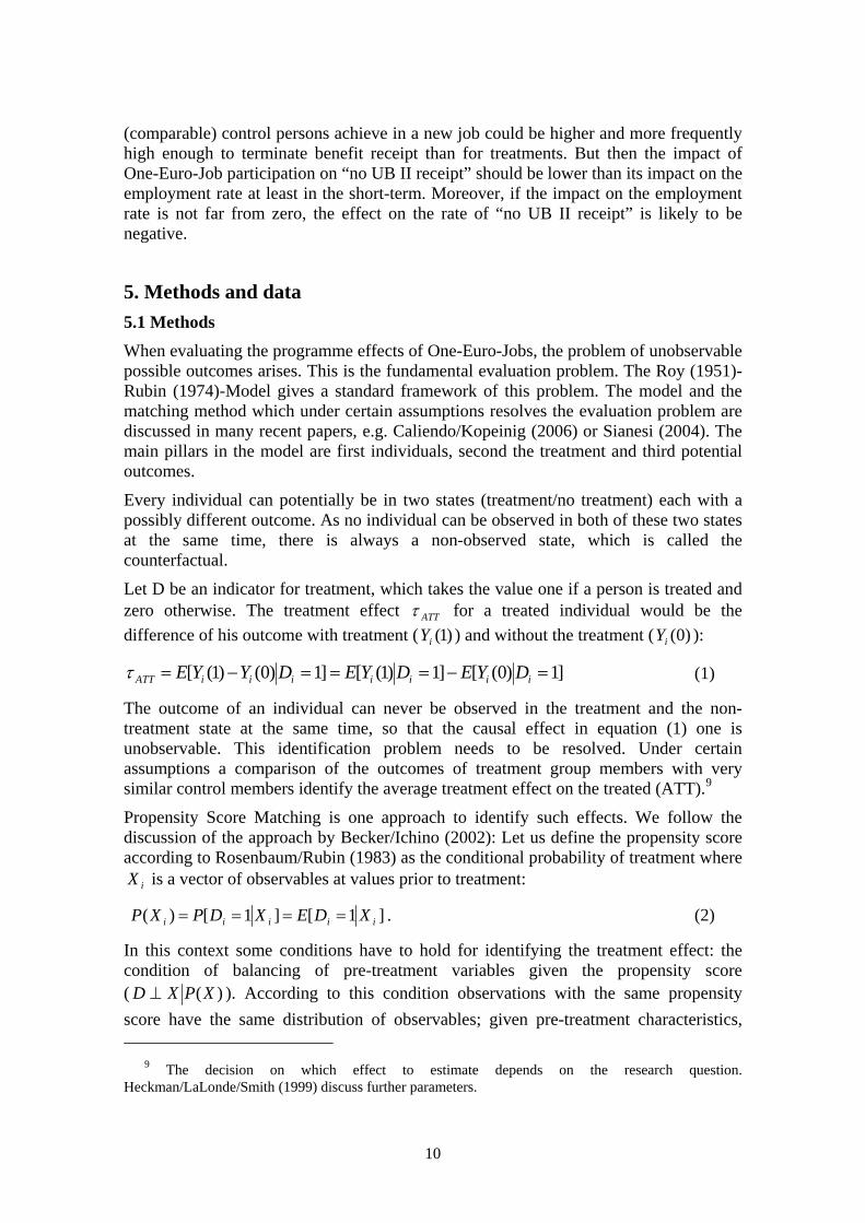
Let D be an indicator for treatment, which takes the value one if a person is treated and zero otherwise. The treatment effect ATTτ for a treated individual would be the difference of his outcome with treatment ( )1(iY ) and without the treatment ( )0(iY ):

]1)0([]1)1([]1)0()1([ =−===−= iiiiiiiATT DYEDYEDYYEτ (1)

The outcome of an individual can never be observed in the treatment and the non-treatment state at the same time, so that the causal effect in equation (1) one is unobservable. This identification problem needs to be resolved. Under certain assumptions a comparison of the outcomes of treatment group members with very similar control members identify the average treatment effect on the treated (ATT).9

Propensity Score Matching is one approach to identify such effects. We follow the discussion of the approach by Becker/Ichino (2002): Let us define the propensity score according to Rosenbaum/Rubin (1983) as the conditional probability of treatment where

iX is a vector of observables at values prior to treatment:

]1[]1[)( iiiii XDEXDPXP ==== . (2)

In this context some conditions have to hold for identifying the treatment effect: the condition of balancing of pre-treatment variables given the propensity score ( )(XPXD ⊥ ). According to this condition observations with the same propensity score have the same distribution of observables; given pre-treatment characteristics,

9 The decision on which effect to estimate depends on the research question. Heckman/LaLonde/Smith (1999) discuss further parameters.

11

treatment is random and treatments and control units do on average not differ with respect to pre-treatment characteristics. Next, there are the conditions of unconfoundedness ( XYY ⊥)0(),1( ) and of unconfoundedness given the propensity score ( )()0(),1( XPYY ⊥ ). Unconfoundedness is also labelled as the conditional independence assumption (CIA) and states that outcomes in case of treatment and non-treatment are independent from actual assignment to treatment given the propensity score.

If treatment is random within cells defined by the vector X , it is also random within such cells defined by the values of propensity score )(XP , which in contrast to X has only one dimension. Given the above conditions, we have

{ }

{ }1|)](,0|)0([)](,1|)1([

)](,1|)0()1([

]1|)0()1([

==−==

=−=

=−=

iiiiiii

iiii

iiiATT

DXPDYEXPDYEE

XPDYYEE

DYYEτ

(3)

The basic idea of the matching estimator is to substitute the unobservable expected outcome without treatment of the treated [ ]1)0( =

ii DYE by an observable expected

outcome of a suitable control group [ ])(,1)0( iii XPDYE = that has the same distribution of the propensity score as the treatment group. To implement a matching estimator, it requires the additional assumption of common support

1)1(0 <=< XDP , (4)

since for individuals whose probability of treatment is either 0 or 1, no counterfactual can be found. Finally, the "stable unit treatment value assumption" (SUTVA) has to be made. It states that the individual's potential outcome only depends on his own participation and not on the treatment status of other individuals. It implies that there are neither general equilibrium nor cross-person effects. In our context there is certainly reason to question this assumption. Since a large number of individuals are treated, we would expect that the outcomes without treatment are also affected, e.g., because in the short-term the number of vacancies is fixed. If treatment leads to vacancies being filled more quickly by treated individuals, the job search process of the non-treated may be prolonged.

We estimate the ATT effects at different points in time after programme start (t=0):

}1|)](,0|)0([{)](,1|)1([ 0,0,0,,0,0,,, ==−== iiitiiititATT DXPDYEEXPDYEτ (5)

As propensity score matching estimators we use nearest neighbour and radius matching imposing common support. Both techniques select for each treatment observation one or more comparison individuals from a potential control group. The following equation defines these estimators10

10 For simplicity we leave away the subscript t for time after programme start.

12

∑ ∑∈ ∈

⎥⎦

⎤⎢⎣

⎡⋅−=

treatedi controlsjjiji

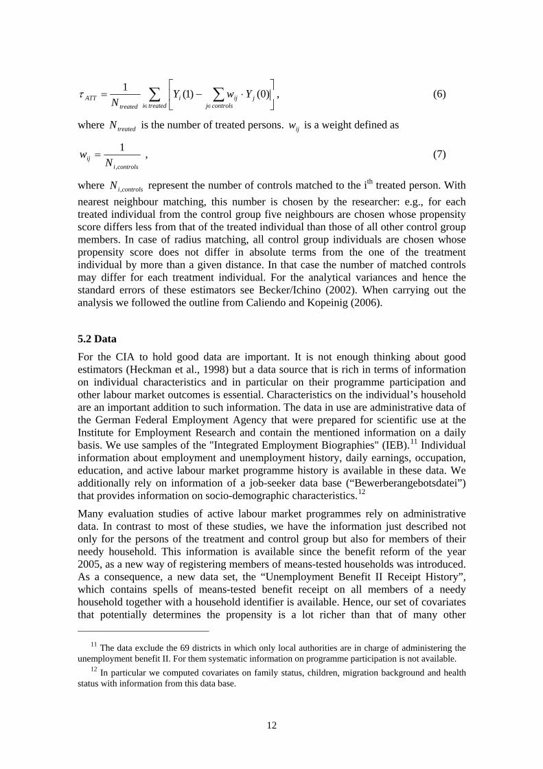
treatedATT YwY

N)0()1(1τ , (6)

where treatedN is the number of treated persons. ijw is a weight defined as

controlsiij N

w,

1= , (7)

where controlsiN , represent the number of controls matched to the ith treated person. With nearest neighbour matching, this number is chosen by the researcher: e.g., for each treated individual from the control group five neighbours are chosen whose propensity score differs less from that of the treated individual than those of all other control group members. In case of radius matching, all control group individuals are chosen whose propensity score does not differ in absolute terms from the one of the treatment individual by more than a given distance. In that case the number of matched controls may differ for each treatment individual. For the analytical variances and hence the standard errors of these estimators see Becker/Ichino (2002). When carrying out the analysis we followed the outline from Caliendo and Kopeinig (2006).

5.2 Data

For the CIA to hold good data are important. It is not enough thinking about good estimators (Heckman et al., 1998) but a data source that is rich in terms of information on individual characteristics and in particular on their programme participation and other labour market outcomes is essential. Characteristics on the individual’s household are an important addition to such information. The data in use are administrative data of the German Federal Employment Agency that were prepared for scientific use at the Institute for Employment Research and contain the mentioned information on a daily basis. We use samples of the "Integrated Employment Biographies" (IEB).11 Individual information about employment and unemployment history, daily earnings, occupation, education, and active labour market programme history is available in these data. We additionally rely on information of a job-seeker data base (“Bewerberangebotsdatei”) that provides information on socio-demographic characteristics.12

Many evaluation studies of active labour market programmes rely on administrative data. In contrast to most of these studies, we have the information just described not only for the persons of the treatment and control group but also for members of their needy household. This information is available since the benefit reform of the year 2005, as a new way of registering members of means-tested households was introduced. As a consequence, a new data set, the “Unemployment Benefit II Receipt History”, which contains spells of means-tested benefit receipt on all members of a needy household together with a household identifier is available. Hence, our set of covariates that potentially determines the propensity is a lot richer than that of many other

11 The data exclude the 69 districts in which only local authorities are in charge of administering the unemployment benefit II. For them systematic information on programme participation is not available.

12 In particular we computed covariates on family status, children, migration background and health status with information from this data base.

13

comparable studies. This is particularly important to justify the Conditional Independence Assumption.

For the treatment group we use the total inflow into One-Euro-Jobs from February to April 2005 of persons who were both registered unemployed and ‘unemployment benefit II’ recipients at the end of January 2005. We only consider unemployed persons aged 15 to 62 years, since older unemployment benefit II recipients do nearly never enter One-Euro-Jobs and we want to avoid keeping persons in the sample who enter their old-age-pension within our observations window. The potential controls stem from a 20 percent random sample of unemployment benefit II recipients who were unemployed at 31st January 2005 and who did not enter the One-Euro-Job programmes from February to April 2005. For the control group members naturally no programme start is available over this period. Therefore, we computed a random programme start for the controls such that it follows the distribution of programme starts of the treatment group over these months and excluded those controls from our analyses who exited from unemployment before the calcuted random programme start.13,14

The data on the outcomes was constructed from two data sources. We used information on contributory employment and whether people are registered as unemployed or as job-seekers from an additional data set, the “Verbleibsnachweise”. These administrative data have one great advantage over the IEB, which also contains such information. They provide the information for a more recent past (e.g., at the time we carried out our analysis the IEB contained information on all contributory employment currently only until the end of the year 2005 and the “Verbleibsnachweise” until May 2007). This is important since we deal with a relatively recent treatment and need to observe outcomes for a sufficiently long period of time after treatment. Combining these data with information on participation of our sample members in ALMPs allows us to compute whether the sample members hold an unsubsidized job of contributory employment at different points in time. We label this variable “regular employment”. By combining these data, the observation window for this outcome contains 20 months after programme start. It is 12 months longer than it would have been, if we had relied on IEB information only. The “Verbleibsnachweise” also allow an observation window of 25 months after programme start for our second outcome variable “neither registered as unemployed nor as job-seeker” which is five months longer than that of the IEB.

13 When computing the random programme start, we took into account differences of the distribution

of programme starts between men and women in East and West Germany. If between 31st of January 2005 and their (computed or true) programme start control or treatment group members already exited from unemployment (e.g., due to some other programme participation), they were dismissed from our samples.

14 The data collected by the UB II agencies at the beginning of the year 2005 is certainly characterised by some measurement error. This is not surprising, given that more than three million needy households with more than six million benefit recipients had to be registered according to the new system. In particular, a new software, “A2ll”, was introduced to register basic information on benefits and other traits of the needy households and their members. Not all UB II agencies provided complete information at the beginning of the year 2005 with this software according to the Statistical Department of the Federal Employment Agency. Therefore to some extent the daily information is not precise. Dates of individual events like the start or end of benefit receipt may not always have been reported or do not precisely reflect the true dates.

14

The information on the third outcome variable “unemployment benefit receipt” stems from another data set, the “Unemployment Benefit II Receipt History” (Leistungshistorik Grundsicherung) and is available for 24 months after programme start.

The sample sizes of treatments and controls are displayed in Table 1 and are considerable. Overall we have more than 70,000 treated. The smallest group are West German women with more than 9,000 participants. For men and women in East or West Germany, there are between 51,000 and 102,000 individuals as potential controls.

6. Results: Average treatment effects on the treated of One-Euro-Jobs 6.1 Implementation We present results for the ATT generally for four groups: men and women in East Germany and in West Germany in order to take into account gender differences and the considerable differences between the East and West German labour markets. Apart from estimating the effects for these four broad samples, we also take into account additional effect heterogeneity. We regard four different age groups (15-24, 25-35, 36-50 and 51-62 years), and Germans without versus Germans with migration background and foreigners and for West Germany also foreigners with different nationalities. Next, we distinguish between three occupational qualification groups (no qualification, apprenticeship/vocational training and higher qualification) and regions with low, intermediate or high unemployment rates. Moreover, we distinguish between people who ended their last regular contributory employment in the year 2004, the years 2001 to 2003, 1992 to 2000 and before 1992 or who were never employed. The sample sizes of these different groups are also presented in Table 1.

We investigate the effects of participation in a One-Euro-Job on three different outcome variables at different points in time after programme start to have a comprehensive insight into the effects of the programme. First, we investigate the effect of participation on the probability of being regularly employed (i.e. unsubsidised contributory employment). Second, we observe whether the persons in our sample are registered as unemployed or job-seeker. The second outcome compared to the first includes participation in active labour market programmes as participants are registered as a job seeker in the majority of cases. Thus, a person who is neither registered as unemployed nor as job-seeking can be a) regularly employed with a working time of 15 hours a week or more, for more than three months and earning sufficiently to live on or b) they have no longer registered as unemployed or job-seeking. Hence, this outcome variable by and large can be interpreted as an indicator for either being employed in a regular and rather stable job or being out of the labour force. Third, we observe whether the household of the person still receives unemployment benefit II. If the household no longer receives UB II, this can be because the household is no longer needy or because the household stopped applying for benefits. For the first possibility there can be several reasons: the person in our sample or other members in the person’s household achieve earnings, such that the household no longer passes the means-test. Various changes in the household composition may also lead to such a result. E.g., a person in our sample moves to another household with sufficient earnings.

15

For each of the analysed groups we estimated one probit model for the probability to participate in One-Euro-Jobs. The covariate sets in these analyses contain personal characteristics (age, nationality, migration status, health indicators, whether the person is single, number of children and qualification), labour market and unemployment benefit history (indicators on unemployment, non-employment, and regular employment periods in the past, UI and UA receipt, past participation in active labour market programmes, characteristics of the last job, whether a person has a minor employment in January 2005), characteristics of the partner (labour market history and qualification) and finally regional characteristics (dummy variables reflecting a classification of the labour market situation developed by Rüb and Werner (2007) and some further controls at district level: unemployment rate, share of long-unemployment in the unemployment pool, ratio between the vacancy and the unemployment stock in January 2005 and their percentage change against the previous year). These characteristics should make it likely that the treatment and control outcomes given the propensity scores differ only due to treatment and hence the unconfoundedness condition holds.

In particular partner characteristics are new in this context, as administrative data are usually weak on such information. Partner characteristics play a role for the employment decisions but also for outcomes like “no receipt of UB II”, e.g., a UB II recipient with a highly in contrast to a low skilled partner is more likely to exit from UB II, when the partner finds a job.

The probit models that we estimated rely on the described set of covariates. Nevertheless, the exact specification of covariate sets differs over the sub-groups. This is first of all because the lower the sample sizes, the broader some variables (e.g., dummy variables for age groups) have to be defined. Second, for the samples that we regard, a number of covariates are highly insignificant and have been deleted.15 In Table 2 we present the coefficients of the four probit models that distinguish between East and West German men and women. The coefficients of probit models that underlie the estimation of the ATTs for the additional subgroups like estimates for different age groups are not presented in this paper; they are available on request.

6.2 Match quality, sensitivity analysis

Rosenbaum Bounds

Our results are based on the assumption of unconfoundedness. If there are any unobserved variables that influence selection into the programme as well as outcome variables of the programme a hidden bias could occur and matching estimators would not be robust. The basic idea behind Rosenbaum Bounds is that the odds of treatment of two matched individuals is one, given that they are characterised by the same

15 We estimated in all cases a probit model with a full variable set and tested whether groups of

variables, e.g., binary variables for the last monthly earnings or the last economic sector were jointly insignificant.

16

observables.16 If there are neglected unobserved factors that influence the participation probabilities though, these odds of treatment could change, e.g., to a value two. With the help of Rosenbaum bounds we can conduct an analysis that determines how sensitive our results are to the influence of an unobserved variable. It shows how strong neglected unobserved factors have to change the odds ratio, so that we overestimate or underestimate the treatment effect.

We computed the Mantel-Haentzel statistic using the Stata Programme “mhbounds” by Becker/Caliendo (2007). We calculated the test statistic QMH for the three outcomes in every observed month after programme start for each sample we considered. Here we report the bounds for the outcome regular employment and for the four broad groups of men and women in East and West Germany in the 20th month only. These are the bounds for nearest neighbour matching with one neighbour and without replacement, as the mhbounds command can only be applied for nearest neighbour matching without replacement or for stratification matching (Becker/Caliendo 2007).

The results are quite sensitive to a potential hidden bias: for men in East and West Germany we find that participation has an insignificant effect on the employment rate after 20 months after programme start. Unobserved factors that lead to odds ratios of 1.05 or 1.10 are sufficient to produce positive or negative significant effects. Effects of East German women are sensitive to a factor of 1.05. Less sensitive are the positive treatment effects of West German women. Unobservable influences that change the odds ratio up to a factor of 1.15 would still be in line with a significant effect at a 10%-level and at a factor of 1.20 they become insignificant.

The results of the sensitivity analysis do not mean that a bias actually exists but that matching results are sensitive to possible deviations from the assumption of unconfoundedness and thus one has to be careful in interpreting the results. However, the treatment effects we obtained are weak und thus it is not surprising that they are sensitive to a potential bias.

Common support

Furthermore for propensity score matching we have to assume that there is a common support which means that the propensity score should lie between zero and one and that the distributions of the propensity score are similar for treatment and control groups. In Figure 1 and 2 the distributions of the propensity score are displayed for men and women in East and West Germany and it becomes obvious that distributions for control and treatment group are very similar.

Sensitivity to matching methods

We estimated the ATT using different matching estimators, nearest neighbour one-to-one matching with and without replacement and nearest neighbour matching with

16 )](1/[)()](1/[)(

jj

ii

XPXPXPXP

−−

would represent the odds of treatment of two matched individuals i and j

with the same covariate vectors.

17

replacement using five neighbours. First, each estimation was carried out without caliper. We estimated the 90th and 99th percentile of the differences between the propensity score of treatments and controls (in absolute terms) in each application. These percentiles were then used as 1st and 2nd caliper leaving out the worst one and ten percent of matches. Furthermore, we estimated the ATT radius-caliper matching with the same percentiles that resulted from nearest neighbour one-to-one matching with replacement. This analysis confirmed that our estimation results are quite stable over the different methods. Deviations tend to be small and only in a few cases and at few points in time they are outside the 95 percent confidence band of the nearest neighbour estimator with five neighbours and with replacement. We present results based on this latter estimator.

Balancing

As we do not condition on all covariates but on the propensity score, we have to check the balancing of the relevant variables. Therefore we applied several measures that give us information on the balancing. The standardised absolute bias measures the distance in the marginal distribution of the covariates. Table 3 displays the standard absolute bias as an average over all covariates. Before matching, the biases for the four broad groups of men and women in East and West Germany range from seven to eleven percent and for the smaller subgroups from about seven up to 22 percent. After matching the bias does not exceed 0.5 percent for the four broad samples and decreases for the subgroups to values between 0.4 and 4.1 percent. However, for most subgroups the bias falls below the value of two percent.

Besides the standardised bias for all covariates we checked the matching quality for single covariates. Tables 4 to 7 display the mean of the covariates for treatments, all controls and matched controls for men and women in East and West Germany. Furthermore, the p-values of a t-test on the hypothesis that the mean of a given covariate is the same for the control and the treatment group are displayed for all covariates. The results demonstrate that after matching there are no significant differences between treatment and control group in any of the variables.

6.3 Overall effects The ATT for the four broad subgroups are shown in Fehler! Verweisquelle konnte nicht gefunden werden. and Table 9 to Table 11. We present the results for the three outcomes regular employment, neither being unemployed nor a job-seeker and no receipt UB II. The results stem from nearest neighbour matching with replacement which matches five individuals from the control group to a treated individual. Standard errors were bootstrapped with 100 repetitions. Note though that Abadie/Imbens (2006) showed that in nearest neighbour matching applications bootstrapped standard errors are not valid in general.

According to Fehler! Verweisquelle konnte nicht gefunden werden. there are locking-in effects in the short: In the first ten months after programme start participants have a lower probability of being regularly employed than comparable non-participants. However, at around six months after the start of the programme the estimated ATTs for the employment rate starts to rise. For women in East and West Germany positive

18

effects appear after 16 (West) and 19 months (East). They are well-determined 20 months after programme start, implying that the employment rate of participants is raised by one percentage point for East German women and 2.7 percentage points for West German women. So for them One-Euro-Jobs participation is effective when it comes to integrating them into the regular labour market.

The policy is ineffective with respect to integrating men into employment during the first 20 months after programme start. And it generally performs worse for participants in East Germany than for participants in West Germany. This may be due to the different economic performance of the two regions and the resulting differences between their labour markets. If there are less job vacancies per unemployed person, locking-in effects as well as positive effects could be smaller. Also other reasons may explain the East-West difference: In the East in contrast to West One-Euro-Jobs are presumably more a relief for long-term non-employed similar to traditional job creation schemes and less a means of improving employability.

The programme effects of the employment outcome are weak in the first 20 months after programme start. This holds in particular for the locking-in effect, if we contrast our findings to those of Caliendo (2005a) on job creation schemes in Germany. They find for example locking-in effects that imply a roughly 20 percentage points reduction of the employment rate at around eight months after programme start for West German public works participants. Our strongest locking-in effect emerged for women in West Germany at minus three percentage points. Since, One-Euro-Job participation lasts frequently six months or less, while public works participation in the above mentioned study rather lasted one year, the length of programme participation is one reason for these differences. Another reason is that needy One-Euro-Job participants are with respect to job finding perspectives a much less positive selection of people from the unemployment pool than the public works participants in the study of Caliendo et al. (2005a). Moreover, the difference could also partly be explained by an incentive effect. Job creation schemes provide participants with a wage, while in One-Euro-Jobs they receive just their UB II and a small compensation. Additionally, working time in One-Euro-Jobs is limited to 30 hours per week which means that there is more time left for participants for job search and thus, locking-in effects are supposed to be reduced.

Regarding the other two outcome variables only negative effects can be observed. That means that participants have a higher probability of being registered unemployed or job seeking and of receiving UB II than comparable non-participants. In the short-run the negative impact on the probability of being neither unemployed nor job-seeking is not surprising since participants are counted as job-seeking while they participate in a One-Euro-Job.

The enduring negative effects on the outcomes not registered as unemployed nor as a job-seeker and no UB II receipt after two years are stronger than the positive ones on the probability of being regularly employed 20 months after programme start. The rate of no UB II receipt is reduced by about two to three percentage points two years after programme start for the participants. Hence, treatment does not avoid UB II receipt. One reason for this result could be that One-Euro-Jobs participants in contrast to comparable persons more frequently find jobs that pay low wages and jobs that are only temporary and in case of women only part-time. If the programme has some threat effect on participants, they may well have reduced their reservations wages as

19

mentioned in section four. In turn, even with a (slight) positive effect on their employment rate after participation ended, One-Euro-Job participation still raises the job-seeker rate of participants. Moreover, the achieved post-participation earnings are often low enough to pass the means-test for UB II receipt. As soon as we have earnings information for a sufficient period of time, we can shed more light on this latter hypothesis.

There may even be more reasons for the negative effects of treatment on the no-job-seeker rate and the no UB II receipt rate. One-Euro-Job participants who have specific difficulties of finding a job may be likely to participate in other active labour market programmes after One-Euro-Job ended, as it is only one of the first steps in achieving employability. Moreover, comparable non-participants maybe more likely to retreat temporarily or permanently from the labour market than participants. E.g., without One-Euro-Job participation young people more frequently enter full-time education and aged people more frequently choose the early retirement option. Finally, changes in household formation may explain the results partly: People who are not subject to activation policies could more frequently change their household composition in a way such that leads the household out of UB II receipt.

We will shed some more light on these issues, in particular on the earnings accepted after participation and reservations wages, when more micro data on the characteristics of the jobs become available. Currently the administrative data provides us only with wage information for the year 2005, but in one year they will offer us the possibility to study earnings about 20 months after programme start. Moreover, panel data of a new household panel survey that oversamples needy households will enable us in the future to regard, whether participation has an impact on reservations wages of participants.

6.4 Effects by age

As previously mentioned young unemployed under the age of 25 years are a special target group of Social Code II and of One-Euro-Jobs in particular. In the first half of the year 2005 among needy unemployed people aged younger than 25 years every fourth person started a One-Euro-Job (Wolff/Hohmeyer 2006). For this age group we observe locking-in effects that are stronger than for any other age group (Table 9 to Table 11). One year after programme start young participants have a probability of being regularly employment that is 2.1 to 2.7 percentage points lower than the probability for comparable benefit recipients who did not participate (Table 9). And these effects are statistically significant.

20 months after programme start the effects on the employment rate are still negative for men in both regions and women in East Germany, while for women in West Germany they are positive. But in all cases they are not well determined. For young women we observe a strong negative effect on neither being unemployed nor job-seeking: they have a ten to eleven percentage points higher probability of being registered as unemployed or job-seeking one year after programme start (Table 10). This may point to the fact that without treatment women under 25 retreat more frequently from the labour market (e.g., due to child rearing or full-time education).

Table 9 shows that locking-in effects for the outcome regular job decline in age, when we regard the effects 12 months after programme start, i.e. the month in which nearly all

20

programme participations are completed. This decline is not surprising. The probability of finding a job tends to decrease over the age groups for needy unemployed people (Wolff/Hohmeyer 2006). A significant positive ATT for the employment rate can be observed for some participant groups above the age of 25 years. For East German women and West German men, treatment raises the employment rate by about one to 1.5 percentage points for the age groups of 36 to 50 and 51 to 62 years. Our estimates also imply a positive and somewhat stronger treatment effect ranging from 2.2 to 4.3 percentage points for West Germans who belong to the age groups 25 to 35, 36 to 50 and 51 to 62 years. The highest effect occurred for West German women aged 25 to 35 years.

Unemployed people aged 50 years or older are a special target group for the work-opportunity programmes, due to their relatively low job finding probability.17 But the policy framework does not generally aim at activating aged unemployed workers. There are specific rules for unemployed people who are older than 57 years. They are allowed to opt for the earliest possible retirement and in turn do not have to sign an integration contract or be available for job offers.18 Moreover, since July 2005 a special One-Euro-Job programme was implemented for this age group. The upper limit for the duration of participation in this special programme is three years. Integrating needy aged workers into the regular labour market is not the only goal of this specific programme, because such an integration often cannot be achieved for above 57 year olds. Thus, it aims at using the older unemployed persons’ professional experience (in jobs of public interest) and provides them with an alternative to being unemployed, which should ideally be combined with a retirement transition (Federal Ministry of Labour and Social Affaires 2005).

Nevertheless, our results show that for needy unemployed people aged 51 to 62 years, treatment can raise their employment rates. Moreover, they are also the age group for which the rate of neither being registered as unemployed nor as a job-seeker decreases considerably due to treatment. 25 months after programme start this rate is about seven to ten percentage points lower than for the matched controls according to our results displayed in Table 10. Hence, participation indeed leads to avoiding or postponing the decision to retreat from the labour market.

Finally, in West Germany 51 to 62 years olds are the only age-group, where we find that the ATT on the rate of no UB II receipt is near zero and hence not (significantly) reduced as for all the other groups (Table 11). The negative estimated ATT on the no UB II receipt rate for East Germans aged 51 to 62 years may be due to the fact that East Germans more frequently than West Germans qualify for early retirement. Wübbeke (2007) shows that aged East German UB II recipients are characterised by higher contribution periods to the statutory pension funds than West Germans. In turn they are

17 Despite the definition as a target group unemployed who are older than 49 were not especially

focussed on by One-Euro-Jobs in 2005 (Wolff/Hohmeyer 2006). 18 This is regulated in Article 65 paragraph 4 SGB II and Article 428 SGB III. The earliest retirement

age for unemployed people was 60 years in the year 2005, provided they have been unemployed for at least 12 months after an age of 58 years and six months (Article 237 Social Code VI). To be eligible for this early retirement option they need to have contributed to the statutory pension insurance funds for at least 15 years and at least eight years in the ten years prior to early retirement. Over the period from 2006 to 2008 though this early retirement age will be gradually increased to 63 years.

21

more likely to fulfil the eligibility criterion for early retirement of a contribution period 15 years or more. Hence, in case of not participating in Euro-Jobs East Germans in contrast to West Germans could more frequently opt for early retirement and exit for this reason from unemployment benefit II receipt.

6.5 Effects by nationality The results for Germans without migration background, Germans with migration background19 and foreigners show the following: In East Germany the estimated ATTs for the employment outcome are small 20 months after programme start; only for women without migration background they are well-determined but nevertheless below one percentage point as displayed by Table 9. The estimated ATTs for East Germans with respect to the outcome “no UB II receipt” point to adverse affects of the programme participation 24 months after programme start: For all groups there is a negative impact (Table 11). It is particularly high in absolute terms for Germans with migration background whose rate of “no UB II receipt” is decreased by more than four percentage points for men and more than six percentage points for women by treatment. It is also high for foreign women in East Germany at more than four percentage points.

For West Germany, the sample sizes allowed us to distinguish between different groups of foreigners. We distinguished between foreigners from the former Soviet Union, Turks and all other foreigners. Our results imply positive effects of treatment on the regular employment rate of Germans with no migration background of 0.7 percentage points for men and 2.2 percentage points for women 20 months after programme start. For West German women with migration background the estimated ATT is considerably higher at nearly seven percentage points. For the different groups of foreigners the effects are not-well determined and only considerable for the group of all other foreigners at values between two and three percentage points 20 months after programme start.

Nevertheless, also in West Germany One-Euro-Job participation does not lead more people out of benefit receipt as the estimated ATTs for the outcome “no UB II receipt” in Table 11 demonstrate. 24 months after programme start the effects are mostly negative and at the same time for Germans, men of Turkish nationality or men and women in the group of other foreigners well determined.

6.6 Effects by occupational qualification Qualification is considered as one crucial factor determining a person’s labour market performance. People with no occupational degree have particular difficulties in finding a job. They could benefit from One-Euro-Job participation by accumulating basic skills and hence by raising their employability. However, for men in both regions and women in East Germany without occupational degree we find that participation is ineffective,

19 The data does not only allow to identify whether persons are of German or foreign nationality. For Germans the job-seeker data base provides also limited information on their migration background. It allows to identify immigrants with German ancestors who became German nationals as well as asylum-seekers and specific types of refugees, who became German nationals. Such people define our group of people with migration background.

22

with near zero or slightly negative effects 20 months after programme start as displayed in Table 9. Only for unskilled West German women the estimated ATT for the employment rate is well determined and positive at 2.5 percentage points.

The ATTs on the employment rate for participants with vocational training and higher occupational degrees tend to be higher than for the unskilled participant group. But only for the highest qualification group and only for women in East and West Germany with ATTs on the employment rate 20 months after programme start of three and more than four percentage points, respectively, the difference to the effect for the unskilled group is substantial (see Table 9). This could reflect that for high-skilled women there is an effect that is rather due to a work-test than due to impacts on employability.20

For the other two outcomes our estimated ATTs are negative for each qualification group men and women in both region and usually well-determined even more than 20 months after programme start (Table 10 and Table 11). Even though for women we found a difference between the impacts on the employment rate of the highest and lowest skill group of roughly two to three percentage points, there is nearly no difference between them when we regard the ATTs on the effects of UB II receipt 24 months after programme start. For East German women the estimated ATTs imply that the rate is reduced by three percentage points for the low skilled group and 3.4 percentage points for the group with the highest skills. The corresponding values for West German women are 3.1 and 2.8 percentage points. We interpret these latter results as evidence that the programme effect for high skilled women implies a reduction in reservation wages. Due to treatment some of them have accepted regular wage offers that they otherwise would have rejected.

6.7 Effects by regional unemployment rate The ATTs for the employment rate do not vary much according to the regional unemployment rate, where the treatment takes place (Table 9). Moreover, the results displayed in Table 9 do not show that participation is more effective for the treated in low compared with higher unemployment regions. We would have regarded this as evidence for the impact of treatment on employability, which at least in low but not necessarily in high unemployment regions should lead to increased employment rates of the treated. But our results are not in line with this hypothesis.

6.8 Effects by time since last employment The One-Euro-Job programme is designed for needy unemployed people who have very low chances of finding a job. People who were out of employment for quite some time are no longer used to regular work-schedules and presumably also no longer motivated to search for jobs. For such people and not for people with a recent experience in the labour market a One-Euro-Job participation should be quite beneficial.

20 Our results are based on a sample of people aged 15 to 62 years. Hence, many sample members with no occupational qualification are still very young and may complete some qualification. Therefore, we estimated also the ATTs for all three qualification groups with a sample of people aged 25 to 62 years. The results of this analysis differ only little from the results on the ATTs that we present. Hence, the qualitative implications of both analyses are by and large the same.

23

The estimated ATTs for the employment outcome displayed in Table 9 are much in favour of the above hypothesis: For men and women in East or West Germany who worked in unsubsidized contributory employment in the year 2004, the programme is ineffective. First of all, the ATTs 12 months after programme start are all negative and point to much higher locking-in effects than for all groups of people who ended their last regular job, before the year 2004. Moreover, even 20 months after programme start the employment rate of those with a regular job in 2004 is (significantly) reduced by about three percentage points for men 1.5 to 2.3 percentage points for women.

In contrast to needy participants with recent employment, treatment is effective for needy people in West Germany if their last regular job ended in the years 2001 to 2003. The treatment effect is 1.8 percentage points for men and 2.7 percentage points for women 20 months after programme start. Both in the East and the West the policy is also effective for the treated whose last job ended between the years 1992 and 2000. They are the group with the highest treatment effect for women in both regions and for men in West Germany. For West German women the treatment effect is quite substantial at about six percentage points 20 months after programme start. The effects for those who were never employed or whose last employment ended before 1992 tend to be lower than for those last employed between 1992 and 2000, but are still positive and for West German women also significant.

Nevertheless, the employment success of participation for some of these groups is not translating into a success in terms of avoiding “UB II receipt” during our observation window of two years after programme start. The estimated ATTs for that outcome are negative for all of them and nearly always significant as shown in Table 11.

7. Summary and conclusions In this paper we analysed the effects of One-Euro-Job participation on the labour market performance of participants. As this is a recently introduced programme, this question has not been studied yet. We consider participants who started a One-Euro-Job in spring 2005 and who have been unemployed and receiving UB II at the end of January 2005. We applied Propensity Score Matching using administrative data of the Federal Employment Agency. These data have several advantages over other data sources. First, we have a large number of observations available that allows us to control for personal heterogeneity. Second, the data include information on household members of benefit recipients, which makes the underlying assumption of conditional independence of the matching estimator more plausible.

We estimated the ATT separately for men and women and East and West Germany due to the different labour market conditions in both German regions. Moreover, we estimated the ATTs distinguishing different groups of participants according to age, migration background, occupational qualification, regional unemployment rate and time since last job. This analysis identifies for which participant groups the programme is effective and there are various reasons to expect that its effectiveness varies between specific groups of people. To have a comprehensive insight in the effects of One-Euro-Jobs on the labour market performance of participants we estimated the ATT for three different outcome variables: the regular employment rate, being neither registered as unemployed nor as job-seeker and no unemployment benefit II receipt.

24

Our results suggest the following: First of all, regarding the outcome regular employment there are locking-in effects of programme participation. This is not surprising for a programme of median duration of six months. However, compared with earlier evaluation results of the public works programme, the locking-in effects are quite small. The likely reason for this is that public works programme participation lasts longer - usually rather for a year - and the participants receive a wage and not only their unemployment benefit and a few Euros more.

Second, regarding our broad samples, only for women and in particular West German women, the participation at some point after programme start raises the employment rate. For East German women we observed that at the end of our observation window, where 20 months after programme start the employment rate is raised by one percentage points. For West German women the corresponding number is 2.7 percentage points and the positive effects occur already four months earlier than for East German women. Compared to the effects on the participants of other programmes such as wage subsidies and within-company training the treatment effects of the One-Euro-Jobs are relatively small. However, this is what can be expected considering the special group of participants in One-Euro-Jobs and bearing in mind that One-Euro-Jobs have to be additional and of public use and thus are not that close to regular employment.

Third, the programme is ineffective with respect to avoiding that people are registered as unemployed or job-seekers and avoiding unemployment benefit II receipt. One potential reason for the latter result is that One-Euro-Job participants find frequently lower paid jobs than the comparable non-participants. In turn the achieved earnings in regular jobs of the One-Euro-Job participants are less frequently sufficient to exit benefit receipt than for the controls. Hence, the programme presumably reduces the reservation wages of participants. Moreover, the non-participants may also more frequently take other routes out of unemployment benefit II receipt than the One-Euro-Jobs participants; e.g. by changing to a household with sufficiently high income or by opting for early retirement in case of older benefit recipients.

Fourth, we find that there are some groups of participants for which One-Euro-Jobs are quite effective, while for others the participation is rather ineffective. A high variation of the effect is observed for participants of different age. For participants aged younger than 25 years the effects on the employment rate tend to be negative and lower than for the other age-groups. Such deviations are particularly high for West German women: The ATT 20 months after programme start is only about one percentage points for the under 25 year olds and between 2.2 and 4.3 percentage points for the other age-groups.

For the employment outcome the ATTs do not vary that much by qualification or the regional unemployment rate. However, they vary considerably with time since last job. For participants who lost their last job in 2004, the treatment effect is negative for both gender and regions 20 months after programme start (the decrease ranges from 1.5 to about three percentage points). For those who lost their job before the year 2004 or who were never regularly employed the opposite is true. They are highest for West German women who lost their last contributory job between 1992 and 2000 at more than five percentage points.

As One-Euro-Jobs are supposed to help the participants to learn the basic preconditions for work, we assumed that they are particularly effective for those unemployed with low employment chances. However, with respect to this hypothesis we find mixed results.

25

On the one hand, participation in a One-Euro-Job is ineffective for participants without an occupational qualification. On the other hand, participation integrates unemployed into the labour market who have not been employed for several years. This is a group that should also have particular difficulties in finding a regular job.

Moreover, the analysis of some specific participant groups implies that locking-in effects tend to be stronger for those unemployed with relatively good chances of finding a job without treatment. For example, locking-in effects are stronger in West than in East Germany. Young unemployed people under the age of 25 years are a special target group of One-Euro-Jobs. Locking-In effects for young unemployed are higher than for any other age group. Even in the medium term, young unemployed people do not benefit from participation in a One-Euro-Job. This gives reason to reconsider the targeting on young unemployed persons.

The policy implications are only partly straightforward: The programme is effective for West German women, and some groups of participants with low chances of finding a job like those aged 51 to 62 years or those who were not recently employed. For a special target group, the under 25 year olds, the One-Euro-Jobs are rather ineffective. Given these results one may argue that the share of participants in the One-Euro-Job programme should become higher for the groups for which it is most effective. Though there are some further effects to be considered: As the programme serves also as a work-test, the adverse effects for some groups of participants may be due to a threat effect that raises the job search efforts already without participation. This is likely for population groups with relatively high chances of finding jobs and a high likelihood of participating in One-Euro-Jobs, e.g., for the under 25 year olds.

There are many questions that future research should shed some light on. First of all, since the available time horizon after programme start is still short, we need to extend the analysis in order to see whether participation is effective in the medium-term. Second, the treatment effects of additional outcomes like earnings and stable versus unstable employment will be quantified. Third, we did not address the question of programme heterogeneity: E.g., is the programme more effective for participants in full-time or part-time One-Euro-Jobs. Finally, our results cannot show whether the programme is effective on a macro basis in the sense of raising the employment rates in regular jobs or reducing the job-seeker rate or rate of means-tested benefit receipt.

26

References Abadie, Alberto, and Guido W. Imbens (2006): “On the Failure of the Bootstrap for

Matching Estimators”, National Bureau of Economic Research Technical Working Paper No. 0325.

Becker, Sascha. O., and Marco Caliendo (2007): “Sensitivity Analysis for Average Treatment Effects”, The Stata Journal, 7(1), 71-83.

Becker, Sascha O., and Andrea Ichino (2002): “Estimation of Average Treatment Effects based on Propensity Scores ”, The Stata Journal, 2(4), 358-377.

Böckmann-Schewe, Lisa, and Anne Röhrig (1997): “Hilfe zur Arbeit. Analyse der Wirksamkeit öffentlich geförderter Beschäftigung der SozialhilfeempfängerInnen”, Düsseldorf.

Blos, Kerstin, and Helmut Rudolph (2005): “Simulationsrechnungen zum Arbeitslosengeld II - Verlierer, aber auch Gewinner”, Institut für Arbeitsmarkt- und Berufsforschung Kurzbericht No. 17/2005, Nürnberg.

Bolvig, Iben, Peter Jensen, and Michael Rosholm (2003): “The Employment Effects of Active Social Policy”, Institute for the Study of Labor Discussion Paper No. 736.

Caliendo, Marco (2006): “Microeconometric Evaluation of Labour Market Policies”, Lecture Notes in Economics and Mathematical Systems No. 568, Springer, Berlin.

Caliendo, Marco, Reinhard Hujer, and Stephan Thomsen (2005a): “The Employment Effect of Job Creation Schemes in Germany: A Microeconometric Evaluation”, Institute for the Study of Labor Discussion Paper, 1512, Bonn.

Caliendo, Marco, Reinhard Hujer, and Stephan Thomsen (2005b): “Individual Employment Effects of Job Creation Schemes in Germany with Respect to Sectoral Heterogeneity”, Institut für Arbeitsmarkt- und Berufsforschung Discussion Paper No 13/2005, Nürnberg.

Caliendo, Marco, and Sabine Kopeinig (2008): “Some Practical Guidance for the Implementation of Propensity Score Matching”, Journal of Economic Surveys, 22(1), 31-72.

Calmfors, Lars (1994): “Active Labour Market Policy and Unemployment - A Framework for the Analysis of Crucial Design Features”, OECD Labour Market and Social Policy Occasional Paper No. 15, Paris.

Calmfors, Lars, Anders Forslund, and Maria Hemström (2002): “Does Active Labour Market Policy Work? Lessons from the Swedish Experiences”, Institute for Labour Market Policy Evaluation Working Paper 2002: 4.

Federal Employment Agency (2005): “Arbeitshilfe zur Umsetzung von Arbeitsgelegenheiten nach § 16 Abs. 3 SGB II” (as at 2nd September 2005).

Federal Employment Agency (2006): “Sozialgesetzbuch Zweites Buch – Grundsicherung für Arbeitsuchende, Jahresbericht 2005: Zahlen, Daten, Fakten”, Nürnberg.

27

Federal Ministry of Labour and Social Affaires (2005): “Merkblatt zur Fortsetzung der Bund-Länder-Initiative zur Bekämpfung der Langzeitarbeitslosigkeit Älterer durch Förderung von bis zu dreijährigen Zusatzjobs (29th Dezember 2005)”.

Gerfin, Michael, and Michael Lechner (2001): “A Microeconometric Evaluation of the Active Labour Market Policy in Switzerland”, The Economic Journal, 112(482), 854-893.

Gueron, Judith M., and Edward Pauly (1991): “From Welfare To Work”, New York.

Hagen, Tobias, and Viktor Steiner (2000): “Von der Finanzierung der Arbeitslosigkeit zur Förderung von Arbeit. Analysen und Empfehlungen zur Arbeitsmarktpolitik in Deutschland”, ZEW Wirtschaftsanalysen, 51, Nomos Verlagsgesellschaft, Baden-Baden.

Heckman, James, Hidehiko Ichimura, Jeffrey Smith, and Petra Todd (1998): “Characterizing Selection Bias Using Experimental Data”, Econometrica, 66(5), 1017-1098.

Heckman, James, Richard LaLonde, and Jeffrey Smith (1999): “The Economics and Econometrics of Active Labor Market Programmes”, in Handbook of Labor Economics, Volume III, ed. By O. Ashenfelter, and D. Card: 1865-2097. Amsterdam, North Holland.

Heinemann, Sarah, Hermann Gartner, and Eva Jozwiak (2006): “Arbeitsförderung für Langzeitarbeitslose. Erste Befunde zu Eingliederungsleistungen des SGB III im Rechtskreis SGB II”, Institut für Arbeitsmarkt- und Berufsforschung Forschungsbericht No. 3/2006, Nürnberg.

Hohmeyer, Katrin, Christoph Schöll, and Joachim Wolff (2006): “Arbeitsgelegenheiten in der Entgeltvariante. Viele Zielgruppen werden noch vernachlässigt”, Institut für Arbeitsmarkt- und Berufsforschung Forschungsbericht No. 22/2006, Nürnberg.

Jacobi, Lena, and Jochen Kluve (2007): “Before and After the Hartz Reforms: The Performance of Active Labour Market Policy in Germany”, Institute for the Study of Labor Discussion Paper, 2100, Bonn.

Kempken, Jürgen, and Achim Trube (1997): “Effektivität und Effizienz sozialorientierter Hilfen zur Arbeit. Lokale Analysen aktivierender Sozialhilfe”, Lit Verlag, Münster.

Lissenburgh, Stephen (2001): “New Deal for the Long-term Unemployed Pilots: Quantitative Evaluation Using Stage 2 Survey”, Employment Service Report ESR 81, Sheffield.

Lodemel, Ivar (2000): “Work Integration through Obligations to Work”, Paper presented at the UWWCLUS Workshop Brussels.

Lodemel, Ivar (2005): “Workfare”, CESifo Dice Report 2/2005.

Ochel, Wolfgang (2004): “Welfare-To-Work Experiences With Specific Work-First Programmes In Selected Countries”, CESifo Working Paper No. 1153, Munich.

Rosenbaum, Paul R., and Donald B. Rubin (1983): “The Central Role of the Propensity Score in Observational Studies for Causal Effects”, Biometrika, 70(1), 41-55.

28

Roy, Andrew D. (1951): “Some Thoughts on The Distribution of Earnings”, Oxford Economic Papers, 3(2), 135-145.

Rubin, Donald B. (1974): “Estimating Causal Effects to Treatments in Randomised and Nonrandomised Studies”, Journal of Educational Psychology, 66(5), 688-701.

Rüb, Felix, and Daniel Werner (2007): “Typisierung von SGB II-Trägern”, Institut für Arbeitsmarkt- und Berufsforschung Forschungsbericht Nr. 1/2007, Nürnberg.

Sianesi, Barbara (2004): “An Evaluation of the Swedish System of Active Labour Programmes in the 1990s”, The Review of Economics and Statistics, 86(1), 133-155.

Trube, Achim (1994): “Fiskalische und soziale Aspekte kommunaler Arbeitsmarktpolitik - Eine vergleichende Analyse sozioökonomischer Effekte von Arbeitslosigkeit und Beschäftigungsförderung vor Ort”, Arbeit und Sozialpolitik, 7-8/94

Voges, Wolfgang, Herbert Jacobs, and Heather Trickey (2001): “Uneven Development - Local Authorities and Workfare in Germany”, in An Offer you Can't Refuse: Workfare in International Perspective, ed. by Lodemel, Ivar, and Heather Trickey: 71-103. The Policy Press, Bristol, United Kingdom.

Wolff, Joachim, and Katrin Hohmeyer (2006): “Förderung von arbeitslosen Personen im Rechtskreis des SGB II durch Arbeitsgelegenheiten: Bislang wenig zielgruppenorientiert”, Institut für Arbeitsmarkt- und Berufsforschung Forschungsbericht No. 10/2006, Nürnberg.

Wübbeke, Christina (2007): “Einmal arm, immer arm?”, Institut für Arbeitsmarkt- und Berufsforschung Kurzbericht No. 14 /2007, Nürnberg.

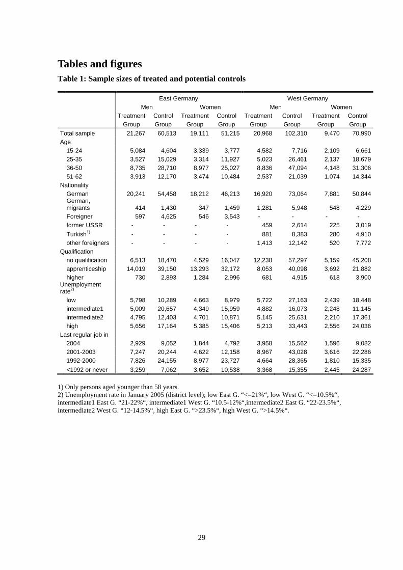
29

Tables and figures Table 1: Sample sizes of treated and potential controls

East Germany West Germany Men Women Men Women Treatment Control Treatment Control Treatment Control Treatment Control Group Group Group Group Group Group Group Group Total sample 21,267 60,513 19,111 51,215 20,968 102,310 9,470 70,990Age 15-24 5,084 4,604 3,339 3,777 4,582 7,716 2,109 6,661 25-35 3,527 15,029 3,314 11,927 5,023 26,461 2,137 18,679 36-50 8,735 28,710 8,977 25,027 8,836 47,094 4,148 31,306 51-62 3,913 12,170 3,474 10,484 2,537 21,039 1,074 14,344Nationality German 20,241 54,458 18,212 46,213 16,920 73,064 7,881 50,844

German, migrants 414 1,430 347 1,459 1,281 5,948 548 4,229

Foreigner 597 4,625 546 3,543 - - - - former USSR - - - - 459 2,614 225 3,019 Turkish1) - - - - 881 8,383 280 4,910 other foreigners - - - - 1,413 12,142 520 7,772Qualification no qualification 6,513 18,470 4,529 16,047 12,238 57,297 5,159 45,208 apprenticeship 14,019 39,150 13,293 32,172 8,053 40,098 3,692 21,882 higher 730 2,893 1,284 2,996 681 4,915 618 3,900Unemployment rate2) low 5,798 10,289 4,663 8,979 5,722 27,163 2,439 18,448 intermediate1 5,009 20,657 4,349 15,959 4,882 16,073 2,248 11,145 intermediate2 4,795 12,403 4,701 10,871 5,145 25,631 2,210 17,361 high 5,656 17,164 5,385 15,406 5,213 33,443 2,556 24,036Last regular job in 2004 2,929 9,052 1,844 4,792 3,958 15,562 1,596 9,082 2001-2003 7,247 20,244 4,622 12,158 8,967 43,028 3,616 22,286 1992-2000 7,826 24,155 8,977 23,727 4,664 28,365 1,810 15,335 <1992 or never 3,259 7,062 3,652 10,538 3,368 15,355 2,445 24,287 1) Only persons aged younger than 58 years. 2) Unemployment rate in January 2005 (district level); low East G. “<=21%“, low West G. “<=10.5%“, intermediate1 East G. “21-22%“, intermediate1 West G. “10.5-12%“,intermediate2 East G. “22-23.5%“, intermediate2 West G. “12-14.5%“, high East G. “>23.5%“, high West G. “>14.5%“.

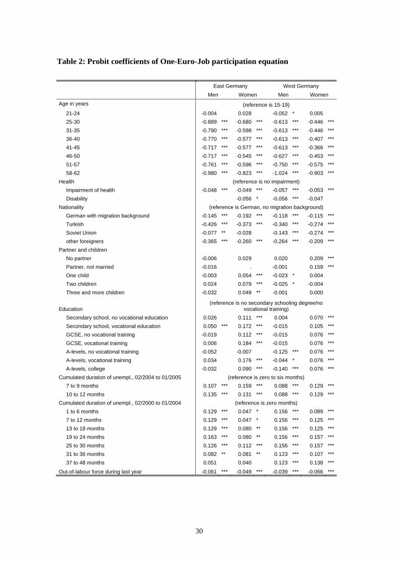
30

Table 2: Probit coefficients of One-Euro-Job participation equation

East Germany West Germany Men Women Men Women Age in years (reference is 15-19) 21-24 -0.004 0.028 -0.052 * 0.005 25-30 -0.889 *** -0.680 *** -0.613 *** -0.446 *** 31-35 -0.790 *** -0.598 *** -0.613 *** -0.446 *** 36-40 -0.770 *** -0.577 *** -0.613 *** -0.407 *** 41-45 -0.717 *** -0.577 *** -0.613 *** -0.366 *** 46-50 -0.717 *** -0.545 *** -0.627 *** -0.453 *** 51-57 -0.761 *** -0.596 *** -0.750 *** -0.575 *** 58-62 -0.980 *** -0.823 *** -1.024 *** -0.903 ***Health (reference is no impairment) Impairment of health -0.048 *** -0.049 *** -0.057 *** -0.053 *** Disability . -0.056 * -0.056 *** -0.047 Nationality (reference is German, no migration background) German with migration background -0.145 *** -0.192 *** -0.118 *** -0.115 *** Turkish -0.426 *** -0.373 *** -0.340 *** -0.274 *** Soviet Union -0.077 ** -0.028 -0.143 *** -0.274 *** other foreigners -0.365 *** -0.260 *** -0.264 *** -0.209 ***Partner and children No partner -0.006 0.029 0.020 0.209 *** Partner, not married -0.016 . -0.001 0.159 *** One child -0.003 0.054 *** -0.023 * 0.004 Two children 0.024 0.079 *** -0.025 * -0.004 Three and more children -0.032 0.049 ** -0.001 0.000

Education (reference is no secondary schooling degree/no

vocational training) Secondary school, no vocational education 0.026 0.111 *** 0.004 0.070 *** Secondary school, vocational education 0.050 *** 0.172 *** -0.015 0.105 *** GCSE, no vocational training -0.019 0.112 *** -0.015 0.076 *** GCSE, vocational training 0.006 0.184 *** -0.015 0.076 *** A-levels, no vocational training -0.052 -0.007 -0.125 *** 0.076 *** A-levels, vocational training 0.034 0.176 *** -0.044 * 0.076 *** A-levels, college -0.032 0.090 *** -0.140 *** 0.076 ***Cumulated duration of unempl., 02/2004 to 01/2005 (reference is zero to six months) 7 to 9 months 0.107 *** 0.159 *** 0.088 *** 0.129 *** 10 to 12 months 0.135 *** 0.131 *** 0.088 *** 0.129 ***Cumulated duration of unempl., 02/2000 to 01/2004 (reference is zero months) 1 to 6 months 0.129 *** 0.047 * 0.156 *** 0.089 *** 7 to 12 months 0.129 *** 0.047 * 0.156 *** 0.125 *** 13 to 18 months 0.129 *** 0.080 ** 0.156 *** 0.125 *** 19 to 24 months 0.163 *** 0.080 ** 0.156 *** 0.157 *** 25 to 30 months 0.126 *** 0.112 *** 0.156 *** 0.157 *** 31 to 36 months 0.082 ** 0.081 ** 0.123 *** 0.107 *** 37 to 48 months 0.051 0.040 0.123 *** 0.138 ***

Out-of-labour force during last year -0.061 *** -0.049 *** -0.039 *** -0.066 ***

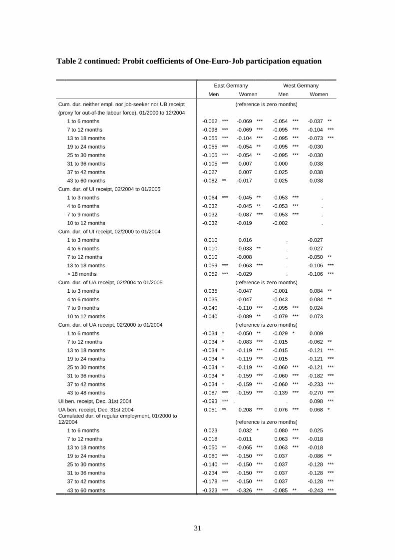
31

Table 2 continued: Probit coefficients of One-Euro-Job participation equation

East Germany West Germany Men Women Men Women

Cum. dur. neither empl. nor job-seeker nor UB receipt (reference is zero months) (proxy for out-of-the labour force), 01/2000 to 12/2004 1 to 6 months -0.062 *** -0.069 *** -0.054 *** -0.037 ** 7 to 12 months -0.098 *** -0.069 *** -0.095 *** -0.104 *** 13 to 18 months -0.055 *** -0.104 *** -0.095 *** -0.073 *** 19 to 24 months -0.055 *** -0.054 ** -0.095 *** -0.030 25 to 30 months -0.105 *** -0.054 ** -0.095 *** -0.030 31 to 36 months -0.105 *** 0.007 0.000 0.038 37 to 42 months -0.027 0.007 0.025 0.038 43 to 60 months -0.082 ** -0.017 0.025 0.038 Cum. dur. of UI receipt, 02/2004 to 01/2005 1 to 3 months -0.064 *** -0.045 ** -0.053 *** . 4 to 6 months -0.032 -0.045 ** -0.053 *** . 7 to 9 months -0.032 -0.087 *** -0.053 *** . 10 to 12 months -0.032 -0.019 -0.002 . Cum. dur. of UI receipt, 02/2000 to 01/2004 1 to 3 months 0.010 0.016 . -0.027 4 to 6 months 0.010 -0.033 ** . -0.027 7 to 12 months 0.010 -0.008 . -0.050 ** 13 to 18 months 0.059 *** 0.063 *** . -0.106 *** > 18 months 0.059 *** -0.029 . -0.106 ***Cum. dur. of UA receipt, 02/2004 to 01/2005 (reference is zero months) 1 to 3 months 0.035 -0.047 -0.001 0.084 ** 4 to 6 months 0.035 -0.047 -0.043 0.084 ** 7 to 9 months -0.040 -0.110 *** -0.095 *** 0.024 10 to 12 months -0.040 -0.089 ** -0.079 *** 0.073 Cum. dur. of UA receipt, 02/2000 to 01/2004 (reference is zero months) 1 to 6 months -0.034 * -0.050 ** -0.029 * 0.009 7 to 12 months -0.034 * -0.083 *** -0.015 -0.062 ** 13 to 18 months -0.034 * -0.119 *** -0.015 -0.121 *** 19 to 24 months -0.034 * -0.119 *** -0.015 -0.121 *** 25 to 30 months -0.034 * -0.119 *** -0.060 *** -0.121 *** 31 to 36 months -0.034 * -0.159 *** -0.060 *** -0.182 *** 37 to 42 months -0.034 * -0.159 *** -0.060 *** -0.233 *** 43 to 48 months -0.087 *** -0.159 *** -0.139 *** -0.270 ***UI ben. receipt, Dec. 31st 2004 -0.093 *** . . 0.098 ***UA ben. receipt, Dec. 31st 2004 0.051 ** 0.208 *** 0.076 *** 0.068 * Cumulated dur. of regular employment, 01/2000 to 12/2004 (reference is zero months) 1 to 6 months 0.023 0.032 * 0.080 *** 0.025 7 to 12 months -0.018 -0.011 0.063 *** -0.018 13 to 18 months -0.050 ** -0.065 *** 0.063 *** -0.018 19 to 24 months -0.080 *** -0.150 *** 0.037 -0.086 ** 25 to 30 months -0.140 *** -0.150 *** 0.037 -0.128 *** 31 to 36 months -0.234 *** -0.150 *** 0.037 -0.128 *** 37 to 42 months -0.178 *** -0.150 *** 0.037 -0.128 ***

43 to 60 months -0.323 *** -0.326 *** -0.085 ** -0.243 ***

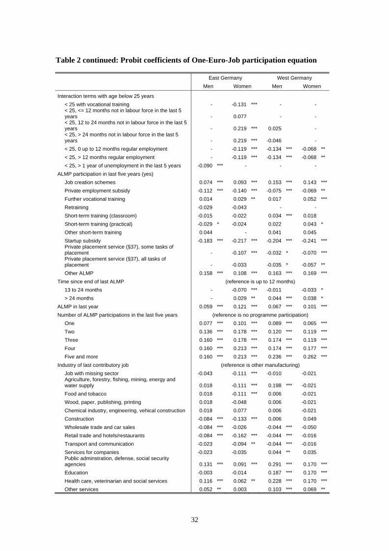
32

Table 2 continued: Probit coefficients of One-Euro-Job participation equation

East Germany West Germany Men Women Men Women

Interaction terms with age below 25 years < 25 with vocational training - -0.131 *** - -

< 25, <= 12 months not in labour force in the last 5 years - 0.077 - -

< 25, 12 to 24 months not in labour force in the last 5 years - 0.219 *** 0.025 -

< 25, > 24 months not in labour force in the last 5 years - 0.219 *** -0.046 -

< 25, 0 up to 12 months regular employment - -0.119 *** -0.134 *** -0.068 ** < 25, > 12 months regular employment - -0.119 *** -0.134 *** -0.068 ** < 25, > 1 year of unemployment in the last 5 years -0.090 *** - - - ALMP participation in last five years (yes) Job creation schemes 0.074 *** 0.093 *** 0.153 *** 0.143 *** Private employment subsidy -0.112 *** -0.140 *** -0.075 *** -0.069 ** Further vocational training 0.014 0.029 ** 0.017 0.052 *** Retraining -0.029 -0.043 - - Short-term training (classroom) -0.015 -0.022 0.034 *** 0.018 Short-term training (practical) -0.029 * -0.024 0.022 0.043 * Other short-term training 0.044 - 0.041 0.045 Startup subsidy -0.183 *** -0.217 *** -0.204 *** -0.241 ***

Private placement service (§37), some tasks of placement - -0.107 *** -0.032 * -0.070 ***

Private placement service (§37), all tasks of placement - -0.033 -0.035 * -0.057 **

Other ALMP 0.158 *** 0.108 *** 0.163 *** 0.169 ***Time since end of last ALMP (reference is up to 12 months) 13 to 24 months - -0.070 *** -0.011 -0.033 * > 24 months - 0.029 ** 0.044 *** 0.038 * ALMP in last year 0.059 *** 0.121 *** 0.067 *** 0.101 ***Number of ALMP participations in the last five years (reference is no programme participation) One 0.077 *** 0.101 *** 0.089 *** 0.065 *** Two 0.136 *** 0.178 *** 0.120 *** 0.119 *** Three 0.160 *** 0.178 *** 0.174 *** 0.119 *** Four 0.160 *** 0.213 *** 0.174 *** 0.177 *** Five and more 0.160 *** 0.213 *** 0.236 *** 0.262 ***Industry of last contributory job (reference is other manufacturing) Job with missing sector -0.043 -0.111 *** -0.010 -0.021

Agriculture, forestry, fishing, mining, energy and water supply 0.018 -0.111 *** 0.198 *** -0.021

Food and tobacco 0.018 -0.111 *** 0.006 -0.021 Wood, paper, publishing, printing 0.018 -0.048 0.006 -0.021 Chemical industry, engineering, vehical construction 0.018 0.077 0.006 -0.021 Construction -0.084 *** -0.133 *** 0.006 0.049 Wholesale trade and car sales -0.084 *** -0.026 -0.044 *** -0.050 Retail trade and hotels/restaurants -0.084 *** -0.162 *** -0.044 *** -0.016 Transport and communication -0.023 -0.094 ** -0.044 *** -0.016 Services for companies -0.023 -0.035 0.044 ** 0.035

Public adminstration, defense, social security agencies 0.131 *** 0.091 *** 0.291 *** 0.170 ***

Education -0.003 -0.014 0.187 *** 0.170 *** Health care, veterinarian and social services 0.116 *** 0.062 ** 0.228 *** 0.170 *** Other services 0.052 ** 0.003 0.103 *** 0.069 **

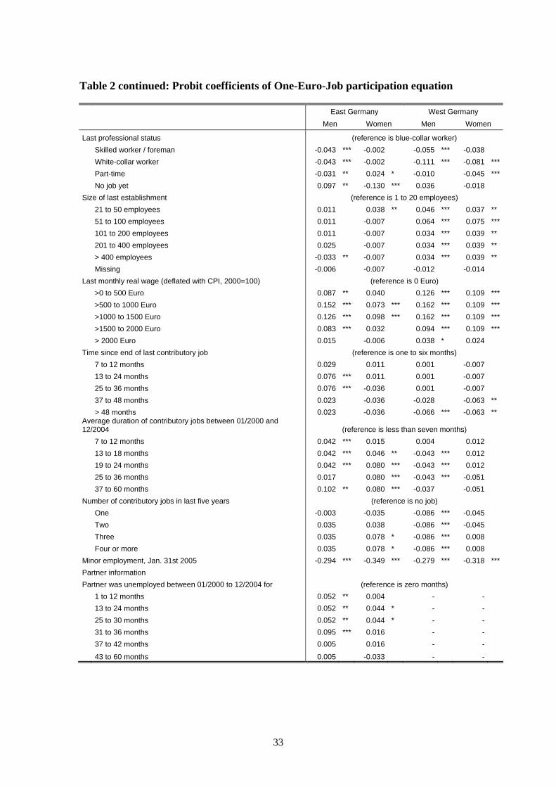
33

Table 2 continued: Probit coefficients of One-Euro-Job participation equation

East Germany West Germany Men Women Men Women

Last professional status (reference is blue-collar worker) Skilled worker / foreman -0.043 *** -0.002 -0.055 *** -0.038 White-collar worker -0.043 *** -0.002 -0.111 *** -0.081 *** Part-time -0.031 ** 0.024 * -0.010 -0.045 *** No job yet 0.097 ** -0.130 *** 0.036 -0.018 Size of last establishment (reference is 1 to 20 employees) 21 to 50 employees 0.011 0.038 ** 0.046 *** 0.037 ** 51 to 100 employees 0.011 -0.007 0.064 *** 0.075 *** 101 to 200 employees 0.011 -0.007 0.034 *** 0.039 ** 201 to 400 employees 0.025 -0.007 0.034 *** 0.039 ** > 400 employees -0.033 ** -0.007 0.034 *** 0.039 ** Missing -0.006 -0.007 -0.012 -0.014 Last monthly real wage (deflated with CPI, 2000=100) (reference is 0 Euro) >0 to 500 Euro 0.087 ** 0.040 0.126 *** 0.109 *** >500 to 1000 Euro 0.152 *** 0.073 *** 0.162 *** 0.109 *** >1000 to 1500 Euro 0.126 *** 0.098 *** 0.162 *** 0.109 *** >1500 to 2000 Euro 0.083 *** 0.032 0.094 *** 0.109 *** > 2000 Euro 0.015 -0.006 0.038 * 0.024 Time since end of last contributory job (reference is one to six months) 7 to 12 months 0.029 0.011 0.001 -0.007 13 to 24 months 0.076 *** 0.011 0.001 -0.007 25 to 36 months 0.076 *** -0.036 0.001 -0.007 37 to 48 months 0.023 -0.036 -0.028 -0.063 ** > 48 months 0.023 -0.036 -0.066 *** -0.063 ** Average duration of contributory jobs between 01/2000 and 12/2004 (reference is less than seven months) 7 to 12 months 0.042 *** 0.015 0.004 0.012 13 to 18 months 0.042 *** 0.046 ** -0.043 *** 0.012 19 to 24 months 0.042 *** 0.080 *** -0.043 *** 0.012 25 to 36 months 0.017 0.080 *** -0.043 *** -0.051 37 to 60 months 0.102 ** 0.080 *** -0.037 -0.051 Number of contributory jobs in last five years (reference is no job) One -0.003 -0.035 -0.086 *** -0.045 Two 0.035 0.038 -0.086 *** -0.045 Three 0.035 0.078 * -0.086 *** 0.008 Four or more 0.035 0.078 * -0.086 *** 0.008 Minor employment, Jan. 31st 2005 -0.294 *** -0.349 *** -0.279 *** -0.318 ***Partner information Partner was unemployed between 01/2000 to 12/2004 for (reference is zero months) 1 to 12 months 0.052 ** 0.004 - - 13 to 24 months 0.052 ** 0.044 * - - 25 to 30 months 0.052 ** 0.044 * - - 31 to 36 months 0.095 *** 0.016 - - 37 to 42 months 0.005 0.016 - -

43 to 60 months 0.005 -0.033 - -

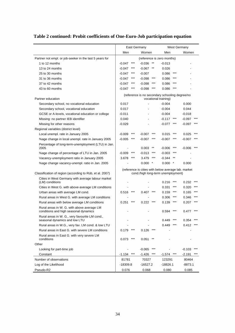
34

Table 2 continued: Probit coefficients of One-Euro-Job participation equation

East Germany West Germany Men Women Men Women

Partner not empl. or job-seeker in the last 5 years for (reference is zero months) 1 to 12 months -0.047 *** -0.036 ** -0.013 - 13 to 24 months -0.047 *** -0.067 ** 0.026 - 25 to 30 months -0.047 *** -0.007 0.086 *** - 31 to 36 months -0.047 *** -0.098 *** 0.086 *** - 37 to 42 months -0.047 *** -0.098 *** 0.086 *** - 43 to 60 months -0.047 *** -0.098 *** 0.086 *** -

Partner education (reference is no secondary schooling degree/no

vocational training) Secondary school, no vocational education 0.017 - -0.004 0.000 Secondary school, vocational education 0.017 - -0.004 0.044 GCSE or A-levels, vocational education or college -0.011 - -0.004 -0.018 Missing: no partner IEB identifier 0.040 - -0.117 *** -0.097 *** Missing for other reasons -0.029 - -0.077 *** -0.097 ***Regional variables (district level) Local unempl. rate in January 2005 -0.009 *** -0.007 *** 0.015 *** 0.025 *** %age change in local unempl. rate in January 2005 -0.005 *** -0.007 *** -0.007 *** -0.007 ***

Percentage of long-term-unemployment (LTU) in Jan. 2005 - 0.003 ** -0.006 *** -0.006 ***

%age change of percentage of LTU in Jan. 2005 -0.009 *** -0.013 *** -0.003 *** - Vacancy-unemployment ratio in January 2005 3.678 *** 3.479 *** -0.344 ** - %age change vacancy-unempl. ratio in Jan. 2005 - 0.000 * 0.000 * 0.000

Classification of region (according to Rüb, et al. 2007) (reference is cities with below average lab. market

cond./high long-term unemployment)

Cities in West Germany with average labour market (LM) conditions - - 0.216 *** 0.232 ***

Cities in West G. with above-average LM conditions - - 0.331 *** 0.320 *** Urban areas with average LM cond. 0.516 *** 0.407 *** 0.159 *** 0.165 *** Rural areas in West G. with average LM conditions - - 0.306 *** 0.346 *** Rural areas with below average LM conditions 0.251 *** 0.222 *** 0.139 *** 0.207 ***

Rural areas in W. G. with above average LM conditions and high seasonal dynamics - - 0.594 *** 0.477 ***

Rural areas in W. G., very favourite LM cond., seasonal dynamics and low LTU - - 0.449 *** 0.354 ***

Rural areas in W.G., very fav. LM cond. & low LTU - - 0.449 *** 0.412 *** Rural areas in East G. with severe LM conditions 0.179 *** 0.126 *** - -

Rural areas in East G. with very severe LM conditions 0.073 *** 0.051 ** - -

Other Looking for part-time job - -0.065 *** - -0.103 *** Constant -1.134 *** -1.426 *** -1.574 *** -2.191 ***Number of observations 81781 70327 123291 80464 Log of the Likelihood -18309.8 -16527.2 -18826.1 -8873.1

Pseudo-R2 0.076 0.068 0.080 0.085

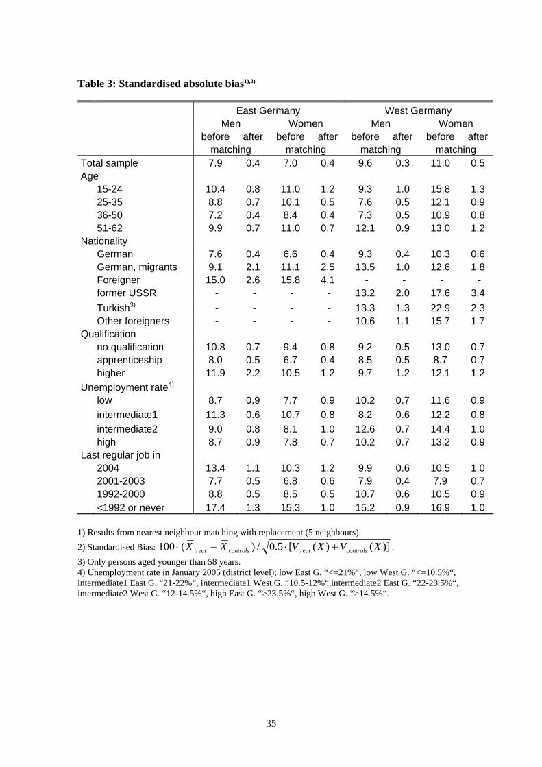
35

Table 3: Standardised absolute bias1),2)

East Germany West Germany Men Women Men Women before after before after before after before after matching matching matching matching Total sample 7.9 0.4 7.0 0.4 9.6 0.3 11.0 0.5 Age 15-24 10.4 0.8 11.0 1.2 9.3 1.0 15.8 1.3 25-35 8.8 0.7 10.1 0.5 7.6 0.5 12.1 0.9 36-50 7.2 0.4 8.4 0.4 7.3 0.5 10.9 0.8 51-62 9.9 0.7 11.0 0.7 12.1 0.9 13.0 1.2 Nationality German 7.6 0.4 6.6 0.4 9.3 0.4 10.3 0.6 German, migrants 9.1 2.1 11.1 2.5 13.5 1.0 12.6 1.8 Foreigner 15.0 2.6 15.8 4.1 - - - - former USSR - - - - 13.2 2.0 17.6 3.4 Turkish3) - - - - 13.3 1.3 22.9 2.3 Other foreigners - - - - 10.6 1.1 15.7 1.7 Qualification no qualification 10.8 0.7 9.4 0.8 9.2 0.5 13.0 0.7 apprenticeship 8.0 0.5 6.7 0.4 8.5 0.5 8.7 0.7 higher 11.9 2.2 10.5 1.2 9.7 1.2 12.1 1.2 Unemployment rate4) low 8.7 0.9 7.7 0.9 10.2 0.7 11.6 0.9 intermediate1 11.3 0.6 10.7 0.8 8.2 0.6 12.2 0.8 intermediate2 9.0 0.8 8.1 1.0 12.6 0.7 14.4 1.0 high 8.7 0.9 7.8 0.7 10.2 0.7 13.2 0.9 Last regular job in 2004 13.4 1.1 10.3 1.2 9.9 0.6 10.5 1.0 2001-2003 7.7 0.5 6.8 0.6 7.9 0.4 7.9 0.7 1992-2000 8.8 0.5 8.5 0.5 10.7 0.6 10.5 0.9 <1992 or never 17.4 1.3 15.3 1.0 15.2 0.9 16.9 1.0

1) Results from nearest neighbour matching with replacement (5 neighbours). 2) Standardised Bias: )]()([5.0/)(100 XVXVXX controlstreatcontrolstreat +⋅−⋅ . 3) Only persons aged younger than 58 years. 4) Unemployment rate in January 2005 (district level); low East G. “<=21%“, low West G. “<=10.5%“, intermediate1 East G. “21-22%“, intermediate1 West G. “10.5-12%“,intermediate2 East G. “22-23.5%“, intermediate2 West G. “12-14.5%“, high East G. “>23.5%“, high West G. “>14.5%“.

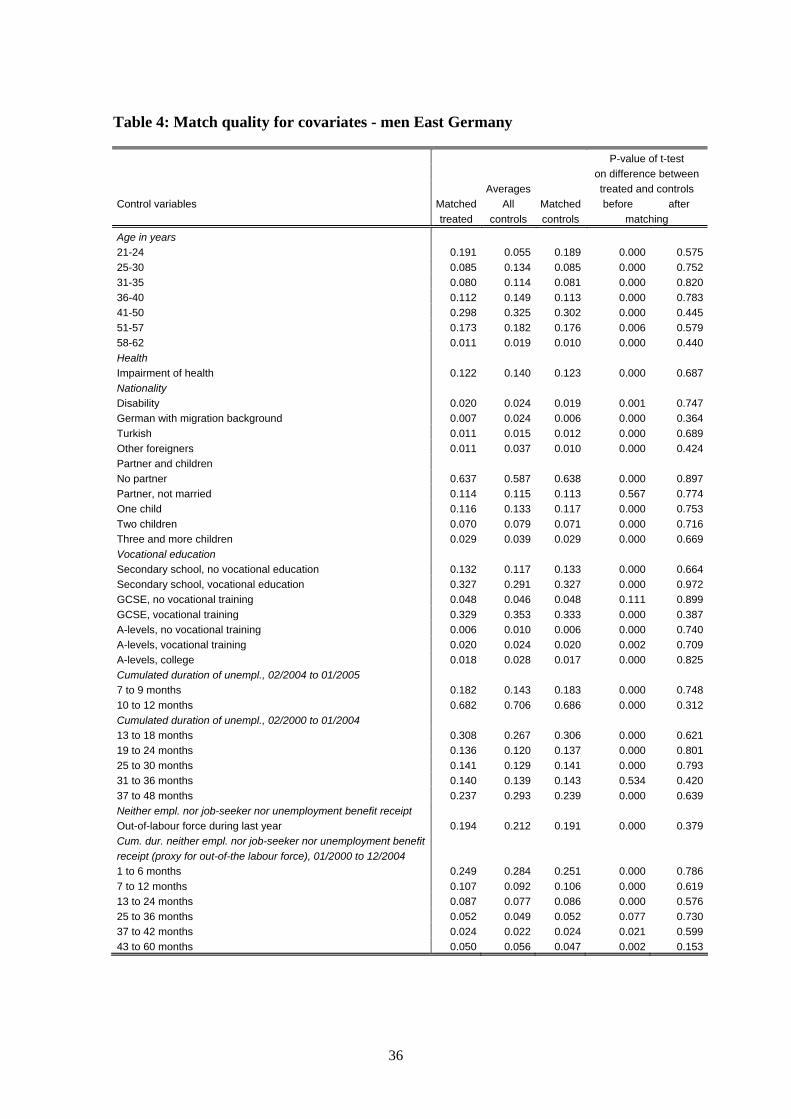
36

Table 4: Match quality for covariates - men East Germany

P-value of t-test on difference between Averages treated and controls Control variables Matched All Matched before after treated controls controls matching

Age in years 21-24 0.191 0.055 0.189 0.000 0.57525-30 0.085 0.134 0.085 0.000 0.75231-35 0.080 0.114 0.081 0.000 0.82036-40 0.112 0.149 0.113 0.000 0.78341-50 0.298 0.325 0.302 0.000 0.44551-57 0.173 0.182 0.176 0.006 0.57958-62 0.011 0.019 0.010 0.000 0.440Health Impairment of health 0.122 0.140 0.123 0.000 0.687Nationality Disability 0.020 0.024 0.019 0.001 0.747German with migration background 0.007 0.024 0.006 0.000 0.364Turkish 0.011 0.015 0.012 0.000 0.689Other foreigners 0.011 0.037 0.010 0.000 0.424Partner and children No partner 0.637 0.587 0.638 0.000 0.897Partner, not married 0.114 0.115 0.113 0.567 0.774One child 0.116 0.133 0.117 0.000 0.753Two children 0.070 0.079 0.071 0.000 0.716Three and more children 0.029 0.039 0.029 0.000 0.669Vocational education Secondary school, no vocational education 0.132 0.117 0.133 0.000 0.664Secondary school, vocational education 0.327 0.291 0.327 0.000 0.972GCSE, no vocational training 0.048 0.046 0.048 0.111 0.899GCSE, vocational training 0.329 0.353 0.333 0.000 0.387A-levels, no vocational training 0.006 0.010 0.006 0.000 0.740A-levels, vocational training 0.020 0.024 0.020 0.002 0.709A-levels, college 0.018 0.028 0.017 0.000 0.825Cumulated duration of unempl., 02/2004 to 01/2005 7 to 9 months 0.182 0.143 0.183 0.000 0.74810 to 12 months 0.682 0.706 0.686 0.000 0.312Cumulated duration of unempl., 02/2000 to 01/2004 13 to 18 months 0.308 0.267 0.306 0.000 0.62119 to 24 months 0.136 0.120 0.137 0.000 0.80125 to 30 months 0.141 0.129 0.141 0.000 0.79331 to 36 months 0.140 0.139 0.143 0.534 0.42037 to 48 months 0.237 0.293 0.239 0.000 0.639Neither empl. nor job-seeker nor unemployment benefit receipt Out-of-labour force during last year 0.194 0.212 0.191 0.000 0.379Cum. dur. neither empl. nor job-seeker nor unemployment benefit receipt (proxy for out-of-the labour force), 01/2000 to 12/2004 1 to 6 months 0.249 0.284 0.251 0.000 0.7867 to 12 months 0.107 0.092 0.106 0.000 0.61913 to 24 months 0.087 0.077 0.086 0.000 0.57625 to 36 months 0.052 0.049 0.052 0.077 0.73037 to 42 months 0.024 0.022 0.024 0.021 0.59943 to 60 months 0.050 0.056 0.047 0.002 0.153

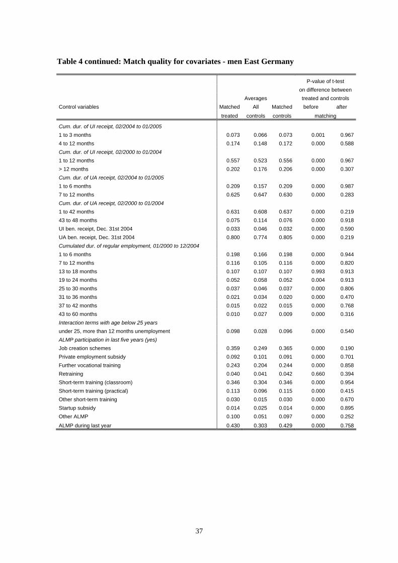
37

Table 4 continued: Match quality for covariates - men East Germany

P-value of t-test on difference between Averages treated and controls Control variables Matched All Matched before after

treated controls controls matching

Cum. dur. of UI receipt, 02/2004 to 01/2005 1 to 3 months 0.073 0.066 0.073 0.001 0.9674 to 12 months 0.174 0.148 0.172 0.000 0.588Cum. dur. of UI receipt, 02/2000 to 01/2004 1 to 12 months 0.557 0.523 0.556 0.000 0.967> 12 months 0.202 0.176 0.206 0.000 0.307Cum. dur. of UA receipt, 02/2004 to 01/2005 1 to 6 months 0.209 0.157 0.209 0.000 0.9877 to 12 months 0.625 0.647 0.630 0.000 0.283Cum. dur. of UA receipt, 02/2000 to 01/2004 1 to 42 months 0.631 0.608 0.637 0.000 0.21943 to 48 months 0.075 0.114 0.076 0.000 0.918UI ben. receipt, Dec. 31st 2004 0.033 0.046 0.032 0.000 0.590UA ben. receipt, Dec. 31st 2004 0.800 0.774 0.805 0.000 0.219Cumulated dur. of regular employment, 01/2000 to 12/2004 1 to 6 months 0.198 0.166 0.198 0.000 0.9447 to 12 months 0.116 0.105 0.116 0.000 0.82013 to 18 months 0.107 0.107 0.107 0.993 0.91319 to 24 months 0.052 0.058 0.052 0.004 0.91325 to 30 months 0.037 0.046 0.037 0.000 0.80631 to 36 months 0.021 0.034 0.020 0.000 0.47037 to 42 months 0.015 0.022 0.015 0.000 0.76843 to 60 months 0.010 0.027 0.009 0.000 0.316Interaction terms with age below 25 years under 25, more than 12 months unemployment 0.098 0.028 0.096 0.000 0.540ALMP participation in last five years (yes) Job creation schemes 0.359 0.249 0.365 0.000 0.190Private employment subsidy 0.092 0.101 0.091 0.000 0.701Further vocational training 0.243 0.204 0.244 0.000 0.858Retraining 0.040 0.041 0.042 0.660 0.394Short-term training (classroom) 0.346 0.304 0.346 0.000 0.954Short-term training (practical) 0.113 0.096 0.115 0.000 0.415Other short-term training 0.030 0.015 0.030 0.000 0.670Startup subsidy 0.014 0.025 0.014 0.000 0.895Other ALMP 0.100 0.051 0.097 0.000 0.252

ALMP during last year 0.430 0.303 0.429 0.000 0.758

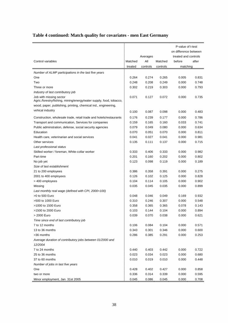
38

Table 4 continued: Match quality for covariates - men East Germany

P-value of t-test on difference between Averages treated and controls Control variables Matched All Matched before after

treated controls controls matching

Number of ALMP participations in the last five years One 0.264 0.274 0.265 0.005 0.831Two 0.248 0.208 0.249 0.000 0.748Three or more 0.302 0.219 0.303 0.000 0.793Industry of last contributory job Job with missing sector 0.071 0.127 0.072 0.000 0.735Agric./forestry/fishing, mining/energy/water supply, food, tobacco, wood, paper, publishing, printing, chemical ind., engineering, vehical industry 0.100 0.087 0.098 0.000 0.483

Construction, wholesale trade, retail trade and hotels/restaurants 0.176 0.239 0.177 0.000 0.786Transport and communication, Services for companies 0.159 0.165 0.160 0.033 0.741Public adminstration, defense, social security agencies 0.079 0.049 0.080 0.000 0.634Education 0.070 0.051 0.070 0.000 0.811Health care, veterinarian and social services 0.041 0.027 0.041 0.000 0.981Other services 0.135 0.111 0.137 0.000 0.715Last professional status Skilled worker / foreman, White-collar worker 0.333 0.406 0.333 0.000 0.982Part-time 0.201 0.160 0.202 0.000 0.802No job yet 0.123 0.098 0.119 0.000 0.189Size of last establishment 21 to 200 employees 0.386 0.358 0.391 0.000 0.2752001 to 400 employees 0.126 0.102 0.125 0.000 0.828> 400 employees 0.104 0.114 0.105 0.000 0.902Missing 0.035 0.045 0.035 0.000 0.899Last monthly real wage (defined with CPI, 2000=100) >0 to 500 Euro 0.048 0.046 0.049 0.169 0.932>500 to 1000 Euro 0.310 0.246 0.307 0.000 0.548>1000 to 1500 Euro 0.358 0.365 0.365 0.078 0.143>1500 to 2000 Euro 0.103 0.144 0.104 0.000 0.894> 2000 Euro 0.039 0.070 0.038 0.000 0.621Time since end of last contributory job 7 to 12 months 0.106 0.084 0.104 0.000 0.57113 to 36 months 0.343 0.301 0.346 0.000 0.600>36 months 0.286 0.385 0.291 0.000 0.253Average duration of contributory jobs between 01/2000 and 12/2004 7 to 24 months 0.440 0.403 0.442 0.000 0.72225 to 36 months 0.023 0.034 0.023 0.000 0.68037 to 60 months 0.010 0.019 0.010 0.000 0.448Number of jobs in last five years One 0.428 0.402 0.427 0.000 0.858two or more 0.336 0.314 0.339 0.000 0.595

Minor employment, Jan. 31st 2005 0.045 0.086 0.045 0.000 0.708

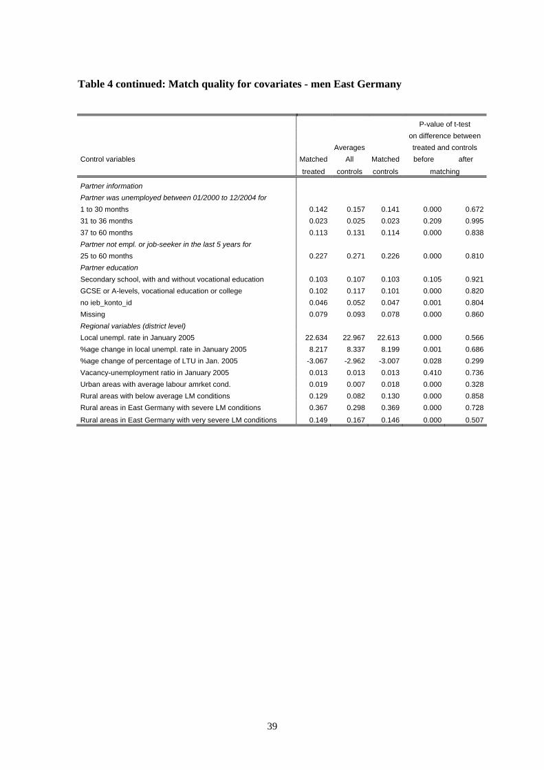
39

Table 4 continued: Match quality for covariates - men East Germany

P-value of t-test on difference between Averages treated and controls Control variables Matched All Matched before after

treated controls controls matching

Partner information Partner was unemployed between 01/2000 to 12/2004 for 1 to 30 months 0.142 0.157 0.141 0.000 0.67231 to 36 months 0.023 0.025 0.023 0.209 0.99537 to 60 months 0.113 0.131 0.114 0.000 0.838Partner not empl. or job-seeker in the last 5 years for 25 to 60 months 0.227 0.271 0.226 0.000 0.810Partner education Secondary school, with and without vocational education 0.103 0.107 0.103 0.105 0.921GCSE or A-levels, vocational education or college 0.102 0.117 0.101 0.000 0.820no ieb_konto_id 0.046 0.052 0.047 0.001 0.804Missing 0.079 0.093 0.078 0.000 0.860Regional variables (district level) Local unempl. rate in January 2005 22.634 22.967 22.613 0.000 0.566%age change in local unempl. rate in January 2005 8.217 8.337 8.199 0.001 0.686%age change of percentage of LTU in Jan. 2005 -3.067 -2.962 -3.007 0.028 0.299Vacancy-unemployment ratio in January 2005 0.013 0.013 0.013 0.410 0.736Urban areas with average labour amrket cond. 0.019 0.007 0.018 0.000 0.328Rural areas with below average LM conditions 0.129 0.082 0.130 0.000 0.858Rural areas in East Germany with severe LM conditions 0.367 0.298 0.369 0.000 0.728

Rural areas in East Germany with very severe LM conditions 0.149 0.167 0.146 0.000 0.507

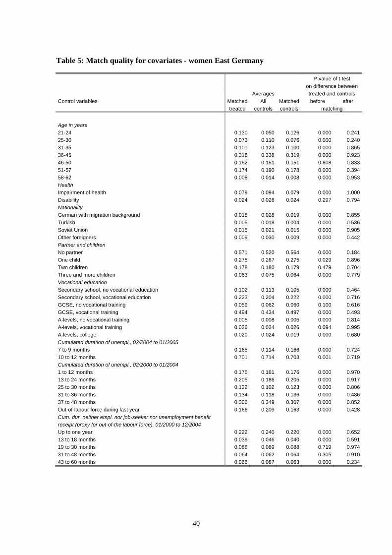
40

Table 5: Match quality for covariates - women East Germany

P-value of t-test on difference between Averages treated and controls Control variables Matched All Matched before after treated controls controls matching

Age in years 21-24 0.130 0.050 0.126 0.000 0.24125-30 0.073 0.110 0.076 0.000 0.24031-35 0.101 0.123 0.100 0.000 0.86536-45 0.318 0.338 0.319 0.000 0.92346-50 0.152 0.151 0.151 0.808 0.83351-57 0.174 0.190 0.178 0.000 0.39458-62 0.008 0.014 0.008 0.000 0.953Health Impairment of health 0.079 0.094 0.079 0.000 1.000Disability 0.024 0.026 0.024 0.297 0.794Nationality German with migration background 0.018 0.028 0.019 0.000 0.855Turkish 0.005 0.018 0.004 0.000 0.536Soviet Union 0.015 0.021 0.015 0.000 0.905Other foreigners 0.009 0.030 0.009 0.000 0.442Partner and children No partner 0.571 0.520 0.564 0.000 0.184One child 0.275 0.267 0.275 0.029 0.896Two children 0.178 0.180 0.179 0.479 0.704Three and more children 0.063 0.075 0.064 0.000 0.779Vocational education Secondary school, no vocational education 0.102 0.113 0.105 0.000 0.464Secondary school, vocational education 0.223 0.204 0.222 0.000 0.716GCSE, no vocational training 0.059 0.062 0.060 0.100 0.616GCSE, vocational training 0.494 0.434 0.497 0.000 0.493A-levels, no vocational training 0.005 0.008 0.005 0.000 0.814A-levels, vocational training 0.026 0.024 0.026 0.094 0.995A-levels, college 0.020 0.024 0.019 0.000 0.680Cumulated duration of unempl., 02/2004 to 01/2005 7 to 9 months 0.165 0.114 0.166 0.000 0.72410 to 12 months 0.701 0.714 0.703 0.001 0.719Cumulated duration of unempl., 02/2000 to 01/2004 1 to 12 months 0.175 0.161 0.176 0.000 0.97013 to 24 months 0.205 0.186 0.205 0.000 0.91725 to 30 months 0.122 0.102 0.123 0.000 0.80631 to 36 months 0.134 0.118 0.136 0.000 0.48637 to 48 months 0.306 0.349 0.307 0.000 0.852Out-of-labour force during last year 0.166 0.209 0.163 0.000 0.428Cum. dur. neither empl. nor job-seeker nor unemployment benefit receipt (proxy for out-of-the labour force), 01/2000 to 12/2004 Up to one year 0.222 0.240 0.220 0.000 0.65213 to 18 months 0.039 0.046 0.040 0.000 0.59119 to 30 months 0.088 0.089 0.088 0.719 0.97431 to 48 months 0.064 0.062 0.064 0.305 0.91043 to 60 months 0.066 0.087 0.063 0.000 0.234

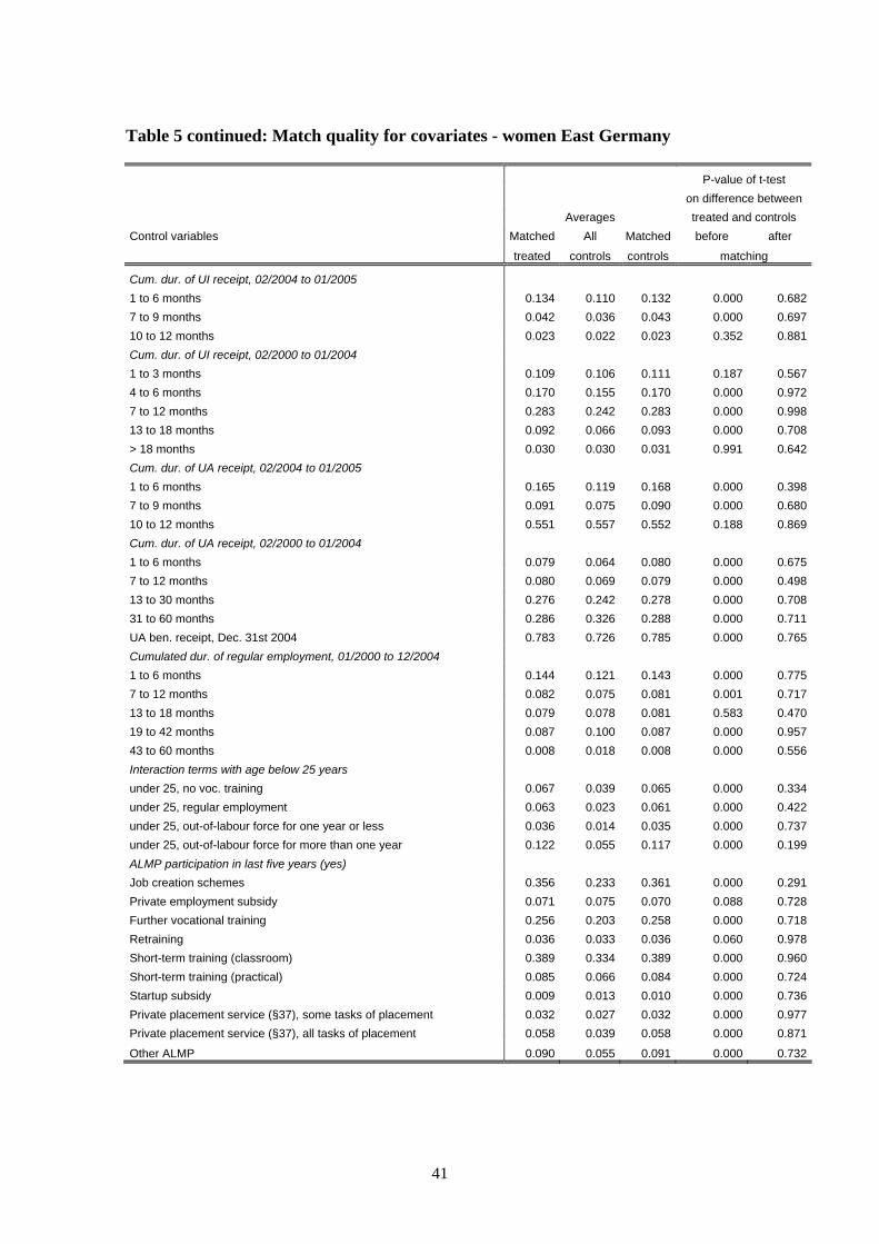
41

Table 5 continued: Match quality for covariates - women East Germany

P-value of t-test on difference between Averages treated and controls Control variables Matched All Matched before after

treated controls controls matching

Cum. dur. of UI receipt, 02/2004 to 01/2005 1 to 6 months 0.134 0.110 0.132 0.000 0.6827 to 9 months 0.042 0.036 0.043 0.000 0.69710 to 12 months 0.023 0.022 0.023 0.352 0.881Cum. dur. of UI receipt, 02/2000 to 01/2004 1 to 3 months 0.109 0.106 0.111 0.187 0.5674 to 6 months 0.170 0.155 0.170 0.000 0.9727 to 12 months 0.283 0.242 0.283 0.000 0.99813 to 18 months 0.092 0.066 0.093 0.000 0.708> 18 months 0.030 0.030 0.031 0.991 0.642Cum. dur. of UA receipt, 02/2004 to 01/2005 1 to 6 months 0.165 0.119 0.168 0.000 0.3987 to 9 months 0.091 0.075 0.090 0.000 0.68010 to 12 months 0.551 0.557 0.552 0.188 0.869Cum. dur. of UA receipt, 02/2000 to 01/2004 1 to 6 months 0.079 0.064 0.080 0.000 0.6757 to 12 months 0.080 0.069 0.079 0.000 0.49813 to 30 months 0.276 0.242 0.278 0.000 0.70831 to 60 months 0.286 0.326 0.288 0.000 0.711UA ben. receipt, Dec. 31st 2004 0.783 0.726 0.785 0.000 0.765Cumulated dur. of regular employment, 01/2000 to 12/2004 1 to 6 months 0.144 0.121 0.143 0.000 0.7757 to 12 months 0.082 0.075 0.081 0.001 0.71713 to 18 months 0.079 0.078 0.081 0.583 0.47019 to 42 months 0.087 0.100 0.087 0.000 0.95743 to 60 months 0.008 0.018 0.008 0.000 0.556Interaction terms with age below 25 years under 25, no voc. training 0.067 0.039 0.065 0.000 0.334under 25, regular employment 0.063 0.023 0.061 0.000 0.422under 25, out-of-labour force for one year or less 0.036 0.014 0.035 0.000 0.737under 25, out-of-labour force for more than one year 0.122 0.055 0.117 0.000 0.199ALMP participation in last five years (yes) Job creation schemes 0.356 0.233 0.361 0.000 0.291Private employment subsidy 0.071 0.075 0.070 0.088 0.728Further vocational training 0.256 0.203 0.258 0.000 0.718Retraining 0.036 0.033 0.036 0.060 0.978Short-term training (classroom) 0.389 0.334 0.389 0.000 0.960Short-term training (practical) 0.085 0.066 0.084 0.000 0.724Startup subsidy 0.009 0.013 0.010 0.000 0.736Private placement service (§37), some tasks of placement 0.032 0.027 0.032 0.000 0.977Private placement service (§37), all tasks of placement 0.058 0.039 0.058 0.000 0.871

Other ALMP 0.090 0.055 0.091 0.000 0.732

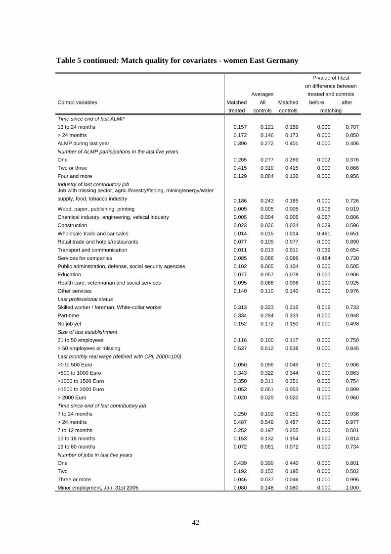
42

Table 5 continued: Match quality for covariates - women East Germany

P-value of t-test on difference between Averages treated and controls Control variables Matched All Matched before after treated controls controls matching Time since end of last ALMP 13 to 24 months 0.157 0.121 0.159 0.000 0.707> 24 months 0.172 0.146 0.173 0.000 0.850ALMP during last year 0.396 0.272 0.401 0.000 0.406Number of ALMP participations in the last five years One 0.265 0.277 0.269 0.002 0.376Two or three 0.415 0.319 0.415 0.000 0.866Four and more 0.129 0.084 0.130 0.000 0.956Industry of last contributory job Job with missing sector, agric./forestry/fishing, mining/energy/water supply, food, tobacco industry 0.186 0.243 0.185 0.000 0.726Wood, paper, publishing, printing 0.005 0.005 0.005 0.906 0.919Chemical industry, engineering, vehical industry 0.005 0.004 0.005 0.067 0.806Construction 0.023 0.026 0.024 0.029 0.596Wholesale trade and car sales 0.014 0.015 0.014 0.461 0.651Retail trade and hotels/restaurants 0.077 0.109 0.077 0.000 0.890Transport and communication 0.011 0.013 0.011 0.039 0.654Services for companies 0.085 0.086 0.086 0.484 0.730Public adminstration, defense, social security agencies 0.102 0.065 0.104 0.000 0.505Education 0.077 0.057 0.078 0.000 0.906Health care, veterinarian and social services 0.095 0.068 0.096 0.000 0.925Other services 0.140 0.110 0.140 0.000 0.976Last professional status Skilled worker / foreman, White-collar worker 0.313 0.323 0.315 0.016 0.733Part-time 0.334 0.294 0.333 0.000 0.948No job yet 0.152 0.172 0.150 0.000 0.498Size of last establishment 21 to 50 employees 0.116 0.100 0.117 0.000 0.750> 50 employees or missing 0.537 0.512 0.538 0.000 0.845Last monthly real wage (defined with CPI, 2000=100) >0 to 500 Euro 0.050 0.056 0.049 0.001 0.906>500 to 1000 Euro 0.343 0.322 0.344 0.000 0.863>1000 to 1500 Euro 0.350 0.311 0.351 0.000 0.754>1500 to 2000 Euro 0.053 0.061 0.053 0.000 0.899> 2000 Euro 0.020 0.029 0.020 0.000 0.960Time since end of last contributory job 7 to 24 months 0.250 0.192 0.251 0.000 0.938> 24 months 0.487 0.549 0.487 0.000 0.9777 to 12 months 0.252 0.197 0.255 0.000 0.50113 to 18 months 0.153 0.132 0.154 0.000 0.81419 to 60 months 0.072 0.081 0.072 0.000 0.734Number of jobs in last five years One 0.439 0.399 0.440 0.000 0.801Two 0.192 0.152 0.195 0.000 0.502Three or more 0.046 0.037 0.046 0.000 0.996Minor employment, Jan. 31st 2005 0.080 0.148 0.080 0.000 1.000

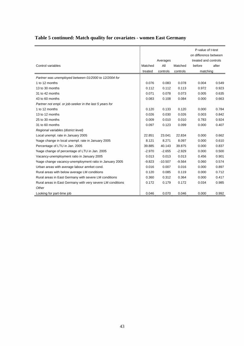
43

Table 5 continued: Match quality for covariates - women East Germany

P-value of t-test on difference between Averages treated and controls Control variables Matched All Matched before after

treated controls controls matching

Partner was unemployed between 01/2000 to 12/2004 for 1 to 12 months 0.076 0.083 0.078 0.004 0.54913 to 30 months 0.112 0.112 0.113 0.972 0.92331 to 42 months 0.071 0.078 0.073 0.005 0.63543 to 60 months 0.083 0.108 0.084 0.000 0.663Partner not empl. or job-seeker in the last 5 years for 1 to 12 months 0.120 0.133 0.120 0.000 0.78413 to 12 months 0.026 0.030 0.026 0.003 0.84225 to 30 months 0.009 0.010 0.010 0.783 0.92431 to 60 months 0.097 0.123 0.099 0.000 0.407Regional variables (district level) Local unempl. rate in January 2005 22.851 23.041 22.834 0.000 0.662%age change in local unempl. rate in January 2005 8.121 8.271 8.097 0.000 0.610Percentage of LTU in Jan. 2005 39.885 40.143 39.875 0.000 0.837%age change of percentage of LTU in Jan. 2005 -2.970 -2.655 -2.929 0.000 0.500Vacancy-unemployment ratio in January 2005 0.013 0.013 0.013 0.456 0.901%age change vacancy-unemployment ratio in January 2005 -9.823 -10.507 -9.564 0.060 0.574Urban areas with average labour amrket cond. 0.016 0.007 0.016 0.000 0.897Rural areas with below average LM conditions 0.120 0.085 0.119 0.000 0.712Rural areas in East Germany with severe LM conditions 0.360 0.312 0.364 0.000 0.417Rural areas in East Germany with very severe LM conditions 0.172 0.179 0.172 0.034 0.985Other

Looking for part-time job 0.046 0.070 0.046 0.000 0.992

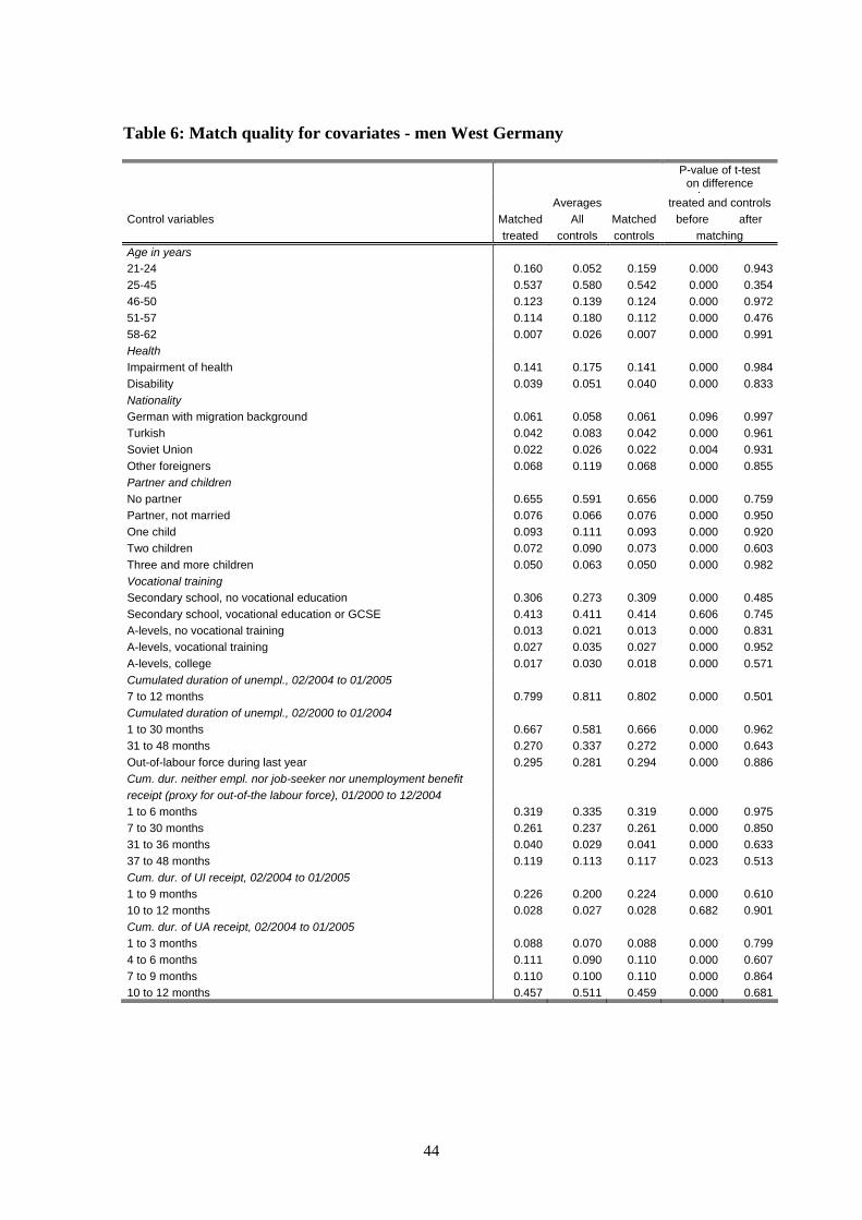
44

Table 6: Match quality for covariates - men West Germany

P-value of t-test on difference

b t Averages treated and controls Control variables Matched All Matched before after treated controls controls matching Age in years 21-24 0.160 0.052 0.159 0.000 0.94325-45 0.537 0.580 0.542 0.000 0.35446-50 0.123 0.139 0.124 0.000 0.97251-57 0.114 0.180 0.112 0.000 0.47658-62 0.007 0.026 0.007 0.000 0.991Health Impairment of health 0.141 0.175 0.141 0.000 0.984Disability 0.039 0.051 0.040 0.000 0.833Nationality German with migration background 0.061 0.058 0.061 0.096 0.997Turkish 0.042 0.083 0.042 0.000 0.961Soviet Union 0.022 0.026 0.022 0.004 0.931Other foreigners 0.068 0.119 0.068 0.000 0.855Partner and children No partner 0.655 0.591 0.656 0.000 0.759Partner, not married 0.076 0.066 0.076 0.000 0.950One child 0.093 0.111 0.093 0.000 0.920Two children 0.072 0.090 0.073 0.000 0.603Three and more children 0.050 0.063 0.050 0.000 0.982Vocational training Secondary school, no vocational education 0.306 0.273 0.309 0.000 0.485Secondary school, vocational education or GCSE 0.413 0.411 0.414 0.606 0.745A-levels, no vocational training 0.013 0.021 0.013 0.000 0.831A-levels, vocational training 0.027 0.035 0.027 0.000 0.952A-levels, college 0.017 0.030 0.018 0.000 0.571Cumulated duration of unempl., 02/2004 to 01/2005 7 to 12 months 0.799 0.811 0.802 0.000 0.501Cumulated duration of unempl., 02/2000 to 01/2004 1 to 30 months 0.667 0.581 0.666 0.000 0.96231 to 48 months 0.270 0.337 0.272 0.000 0.643Out-of-labour force during last year 0.295 0.281 0.294 0.000 0.886Cum. dur. neither empl. nor job-seeker nor unemployment benefit receipt (proxy for out-of-the labour force), 01/2000 to 12/2004 1 to 6 months 0.319 0.335 0.319 0.000 0.9757 to 30 months 0.261 0.237 0.261 0.000 0.85031 to 36 months 0.040 0.029 0.041 0.000 0.63337 to 48 months 0.119 0.113 0.117 0.023 0.513Cum. dur. of UI receipt, 02/2004 to 01/2005 1 to 9 months 0.226 0.200 0.224 0.000 0.61010 to 12 months 0.028 0.027 0.028 0.682 0.901Cum. dur. of UA receipt, 02/2004 to 01/2005 1 to 3 months 0.088 0.070 0.088 0.000 0.7994 to 6 months 0.111 0.090 0.110 0.000 0.6077 to 9 months 0.110 0.100 0.110 0.000 0.86410 to 12 months 0.457 0.511 0.459 0.000 0.681

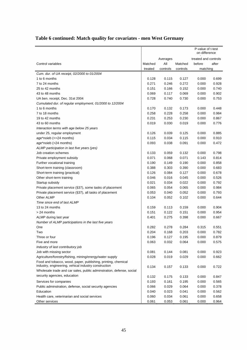
45

Table 6 continued: Match quality for covariates - men West Germany

P-value of t-test on difference

b t Averages treated and controls Control variables Matched All Matched before after treated controls controls matching Cum. dur. of UA receipt, 02/2000 to 01/2004 1 to 6 months 0.128 0.115 0.127 0.000 0.6997 to 24 months 0.271 0.246 0.272 0.000 0.92825 to 42 months 0.151 0.166 0.152 0.000 0.74043 to 48 months 0.069 0.117 0.069 0.000 0.902UA ben. receipt, Dec. 31st 2004 0.728 0.740 0.730 0.000 0.753Cumulated dur. of regular employment, 01/2000 to 12/2004 1 to 6 months 0.170 0.132 0.173 0.000 0.4487 to 18 months 0.258 0.228 0.258 0.000 0.98419 to 42 months 0.231 0.253 0.230 0.000 0.86743 to 60 months 0.019 0.030 0.019 0.000 0.776Interaction terms with age below 25 years under 25, regular employment 0.126 0.039 0.125 0.000 0.885age*noieb (<=24 months) 0.115 0.034 0.115 0.000 0.910age*noieb (>24 months) 0.093 0.038 0.091 0.000 0.472ALMP participation in last five years (yes) Job creation schemes 0.133 0.059 0.132 0.000 0.798Private employment subsidy 0.071 0.068 0.071 0.143 0.814Further vocational training 0.190 0.149 0.190 0.000 0.858Short-term training (classroom) 0.388 0.303 0.390 0.000 0.683Short-term training (practical) 0.126 0.084 0.127 0.000 0.678Other short-term training 0.046 0.016 0.045 0.000 0.526Startup subsidy 0.021 0.034 0.022 0.000 0.792Private placement service (§37), some tasks of placement 0.065 0.054 0.065 0.000 0.984Private placement service (§37), all tasks of placement 0.053 0.040 0.052 0.000 0.793Other ALMP 0.104 0.052 0.102 0.000 0.644Time since end of last ALMP 13 to 24 months 0.159 0.113 0.159 0.000 0.904> 24 months 0.151 0.122 0.151 0.000 0.954ALMP during last year 0.401 0.275 0.398 0.000 0.667Number of ALMP participations in the last five years One 0.282 0.278 0.284 0.315 0.551Two 0.204 0.168 0.203 0.000 0.782Three or four 0.196 0.127 0.195 0.000 0.879Five and more 0.063 0.032 0.064 0.000 0.575Industry of last contributory job Job with missing sector 0.081 0.144 0.081 0.000 0.923Agriculture/forestry/fishing, mining/energy/water supply 0.028 0.019 0.029 0.000 0.662Food and tobacco, wood, paper, publishing, printing, chemical industry, engineering, vehical industry construction 0.134 0.157 0.133 0.000 0.722Wholesale trade and car sales, public adminstration, defense, social security agencies, education 0.132 0.175 0.133 0.000 0.847Services for companies 0.193 0.161 0.195 0.000 0.565Public adminstration, defense, social security agencies 0.066 0.029 0.064 0.000 0.378Education 0.040 0.023 0.041 0.000 0.562Health care, veterinarian and social services 0.060 0.034 0.061 0.000 0.658Other services 0.061 0.053 0.061 0.000 0.964

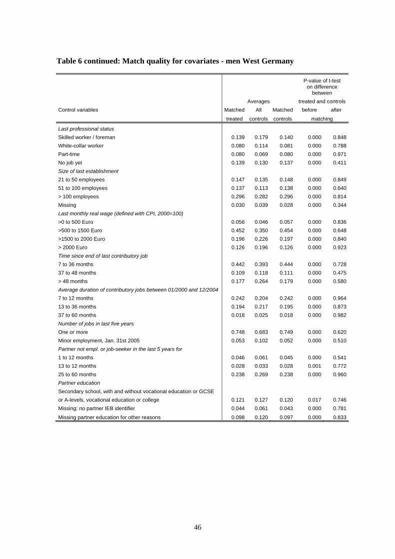
46

Table 6 continued: Match quality for covariates - men West Germany

P-value of t-test

on difference

between Averages treated and controls Control variables Matched All Matched before after

treated controls controls matching

Last professional status Skilled worker / foreman 0.139 0.179 0.140 0.000 0.848White-collar worker 0.080 0.114 0.081 0.000 0.788Part-time 0.080 0.069 0.080 0.000 0.971No job yet 0.139 0.130 0.137 0.000 0.411Size of last establishment 21 to 50 employees 0.147 0.135 0.148 0.000 0.84951 to 100 employees 0.137 0.113 0.138 0.000 0.640> 100 employees 0.296 0.282 0.296 0.000 0.814Missing 0.030 0.039 0.028 0.000 0.344Last monthly real wage (defined with CPI, 2000=100) >0 to 500 Euro 0.056 0.046 0.057 0.000 0.836>500 to 1500 Euro 0.452 0.350 0.454 0.000 0.648>1500 to 2000 Euro 0.196 0.226 0.197 0.000 0.840> 2000 Euro 0.126 0.196 0.126 0.000 0.923Time since end of last contributory job 7 to 36 months 0.442 0.393 0.444 0.000 0.72837 to 48 months 0.109 0.118 0.111 0.000 0.475> 48 months 0.177 0.264 0.179 0.000 0.580Average duration of contributory jobs between 01/2000 and 12/2004 7 to 12 months 0.242 0.204 0.242 0.000 0.96413 to 36 months 0.194 0.217 0.195 0.000 0.87337 to 60 months 0.018 0.025 0.018 0.000 0.982Number of jobs in last five years One or more 0.748 0.683 0.749 0.000 0.620Minor employment, Jan. 31st 2005 0.053 0.102 0.052 0.000 0.510Partner not empl. or job-seeker in the last 5 years for 1 to 12 months 0.046 0.061 0.045 0.000 0.54113 to 12 months 0.028 0.033 0.028 0.001 0.77225 to 60 months 0.238 0.269 0.238 0.000 0.960Partner education Secondary school, with and without vocational education or GCSE or A-levels, vocational education or college 0.121 0.127 0.120 0.017 0.746Missing: no partner IEB identifier 0.044 0.061 0.043 0.000 0.781

Missing partner education for other reasons 0.098 0.120 0.097 0.000 0.833

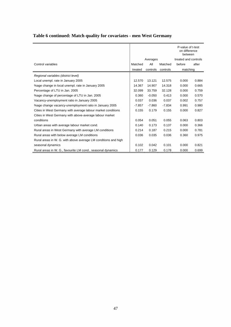
47

Table 6 continued: Match quality for covariates - men West Germany

P-value of t-test

on difference

between Averages treated and controls Control variables Matched All Matched before after

treated controls controls matching

Regional variables (district level) Local unempl. rate in January 2005 12.570 13.121 12.575 0.000 0.884%age change in local unempl. rate in January 2005 14.367 14.907 14.318 0.000 0.665Percentage of LTU in Jan. 2005 32.099 33.759 32.128 0.000 0.759%age change of percentage of LTU in Jan. 2005 0.360 -0.050 0.413 0.000 0.570Vacancy-unemployment ratio in January 2005 0.037 0.036 0.037 0.002 0.757%age change vacancy-unemployment ratio in January 2005 -7.857 -7.860 -7.834 0.991 0.980Cities in West Germany with average labour market conditions 0.155 0.179 0.155 0.000 0.827Cities in West Germany with above-average labour market conditions 0.054 0.051 0.055 0.063 0.803Urban areas with average labour market cond. 0.140 0.173 0.137 0.000 0.366Rural areas in West Germany with average LM conditions 0.214 0.187 0.215 0.000 0.781Rural areas with below average LM conditions 0.036 0.035 0.036 0.360 0.975Rural areas in W. G. with above average LM conditions and high seasonal dynamics 0.102 0.042 0.101 0.000 0.821

Rural areas in W. G., favourite LM cond., seasonal dynamics 0.177 0.129 0.178 0.000 0.699

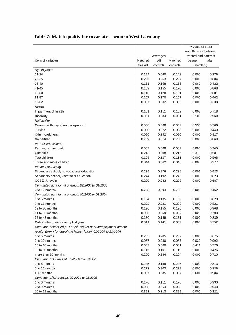
48

Table 7: Match quality for covariates - women West Germany

P-value of t-test on difference between Averages treated and controls Control variables Matched All Matched before after treated controls controls matching Age in years 21-24 0.154 0.060 0.148 0.000 0.27625-35 0.226 0.263 0.227 0.000 0.88436-40 0.151 0.158 0.155 0.060 0.42241-45 0.169 0.155 0.170 0.000 0.86846-50 0.118 0.128 0.121 0.005 0.58151-57 0.107 0.170 0.107 0.000 0.96258-62 0.007 0.032 0.005 0.000 0.338Health Impairment of health 0.101 0.111 0.102 0.003 0.718Disability 0.031 0.034 0.031 0.100 0.960Nationality German with migration background 0.058 0.060 0.059 0.530 0.706Turkish 0.030 0.072 0.028 0.000 0.440Other foreigners 0.080 0.152 0.080 0.000 0.927No partner 0.759 0.614 0.758 0.000 0.868Partner and children Partner, not married 0.082 0.068 0.082 0.000 0.945One child 0.213 0.208 0.216 0.313 0.581Two children 0.109 0.127 0.111 0.000 0.568Three and more children 0.044 0.062 0.046 0.000 0.377Vocational training Secondary school, no vocational education 0.289 0.276 0.289 0.006 0.923Secondary school, vocational education 0.244 0.192 0.245 0.000 0.823GCSE, A-levels 0.290 0.243 0.293 0.000 0.687Cumulated duration of unempl., 02/2004 to 01/2005 7 to 12 months 0.723 0.594 0.728 0.000 0.462Cumulated duration of unempl., 02/2000 to 01/2004 1 to 6 months 0.164 0.135 0.163 0.000 0.8207 to 18 months 0.292 0.221 0.293 0.000 0.82119 to 30 months 0.196 0.155 0.196 0.000 0.96831 to 36 months 0.065 0.059 0.067 0.028 0.70337 to 48 months 0.130 0.149 0.131 0.000 0.839Out-of-labour force during last year 0.341 0.441 0.339 0.000 0.752Cum. dur. neither empl. nor job-seeker nor unemployment benefit receipt (proxy for out-of-the labour force), 01/2000 to 12/2004 1 to 6 months 0.235 0.205 0.232 0.000 0.6757 to 12 months 0.087 0.080 0.087 0.032 0.99213 to 18 months 0.062 0.060 0.061 0.411 0.72619 to 30 months 0.115 0.101 0.119 0.000 0.426more than 30 months 0.266 0.344 0.264 0.000 0.720Cum. dur. of UI receipt, 02/2000 to 01/2004 1 to 6 months 0.225 0.159 0.226 0.000 0.8137 to 12 months 0.273 0.203 0.272 0.000 0.886> 12 months 0.087 0.085 0.087 0.601 0.984Cum. dur. of UA receipt, 02/2004 to 01/2005 1 to 6 months 0.176 0.111 0.176 0.000 0.9307 to 9 months 0.088 0.064 0.088 0.000 0.94310 to 12 months 0.363 0.313 0.365 0.000 0.821

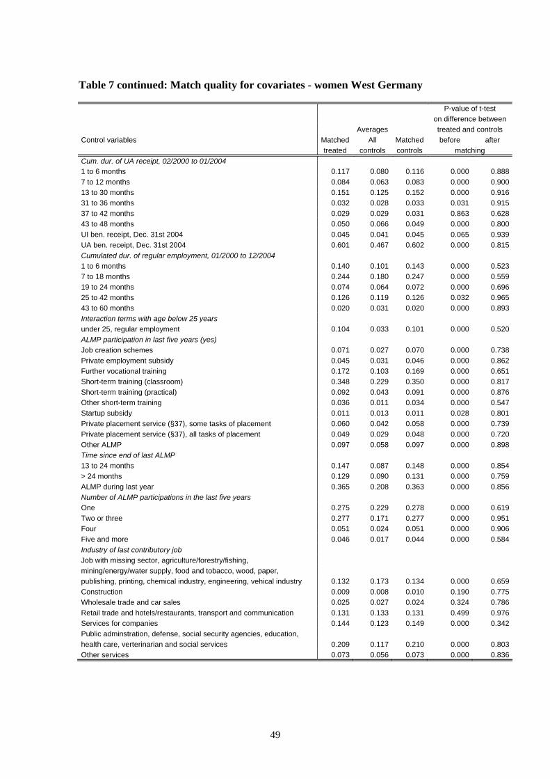
49

Table 7 continued: Match quality for covariates - women West Germany

P-value of t-test on difference between Averages treated and controls Control variables Matched All Matched before after treated controls controls matching Cum. dur. of UA receipt, 02/2000 to 01/2004 1 to 6 months 0.117 0.080 0.116 0.000 0.8887 to 12 months 0.084 0.063 0.083 0.000 0.90013 to 30 months 0.151 0.125 0.152 0.000 0.91631 to 36 months 0.032 0.028 0.033 0.031 0.91537 to 42 months 0.029 0.029 0.031 0.863 0.62843 to 48 months 0.050 0.066 0.049 0.000 0.800UI ben. receipt, Dec. 31st 2004 0.045 0.041 0.045 0.065 0.939UA ben. receipt, Dec. 31st 2004 0.601 0.467 0.602 0.000 0.815Cumulated dur. of regular employment, 01/2000 to 12/2004 1 to 6 months 0.140 0.101 0.143 0.000 0.5237 to 18 months 0.244 0.180 0.247 0.000 0.55919 to 24 months 0.074 0.064 0.072 0.000 0.69625 to 42 months 0.126 0.119 0.126 0.032 0.96543 to 60 months 0.020 0.031 0.020 0.000 0.893Interaction terms with age below 25 years under 25, regular employment 0.104 0.033 0.101 0.000 0.520ALMP participation in last five years (yes) Job creation schemes 0.071 0.027 0.070 0.000 0.738Private employment subsidy 0.045 0.031 0.046 0.000 0.862Further vocational training 0.172 0.103 0.169 0.000 0.651Short-term training (classroom) 0.348 0.229 0.350 0.000 0.817Short-term training (practical) 0.092 0.043 0.091 0.000 0.876Other short-term training 0.036 0.011 0.034 0.000 0.547Startup subsidy 0.011 0.013 0.011 0.028 0.801Private placement service (§37), some tasks of placement 0.060 0.042 0.058 0.000 0.739Private placement service (§37), all tasks of placement 0.049 0.029 0.048 0.000 0.720Other ALMP 0.097 0.058 0.097 0.000 0.898Time since end of last ALMP 13 to 24 months 0.147 0.087 0.148 0.000 0.854> 24 months 0.129 0.090 0.131 0.000 0.759ALMP during last year 0.365 0.208 0.363 0.000 0.856Number of ALMP participations in the last five years One 0.275 0.229 0.278 0.000 0.619Two or three 0.277 0.171 0.277 0.000 0.951Four 0.051 0.024 0.051 0.000 0.906Five and more 0.046 0.017 0.044 0.000 0.584Industry of last contributory job Job with missing sector, agriculture/forestry/fishing, mining/energy/water supply, food and tobacco, wood, paper, publishing, printing, chemical industry, engineering, vehical industry 0.132 0.173 0.134 0.000 0.659Construction 0.009 0.008 0.010 0.190 0.775Wholesale trade and car sales 0.025 0.027 0.024 0.324 0.786Retail trade and hotels/restaurants, transport and communication 0.131 0.133 0.131 0.499 0.976Services for companies 0.144 0.123 0.149 0.000 0.342Public adminstration, defense, social security agencies, education, health care, verterinarian and social services 0.209 0.117 0.210 0.000 0.803Other services 0.073 0.056 0.073 0.000 0.836

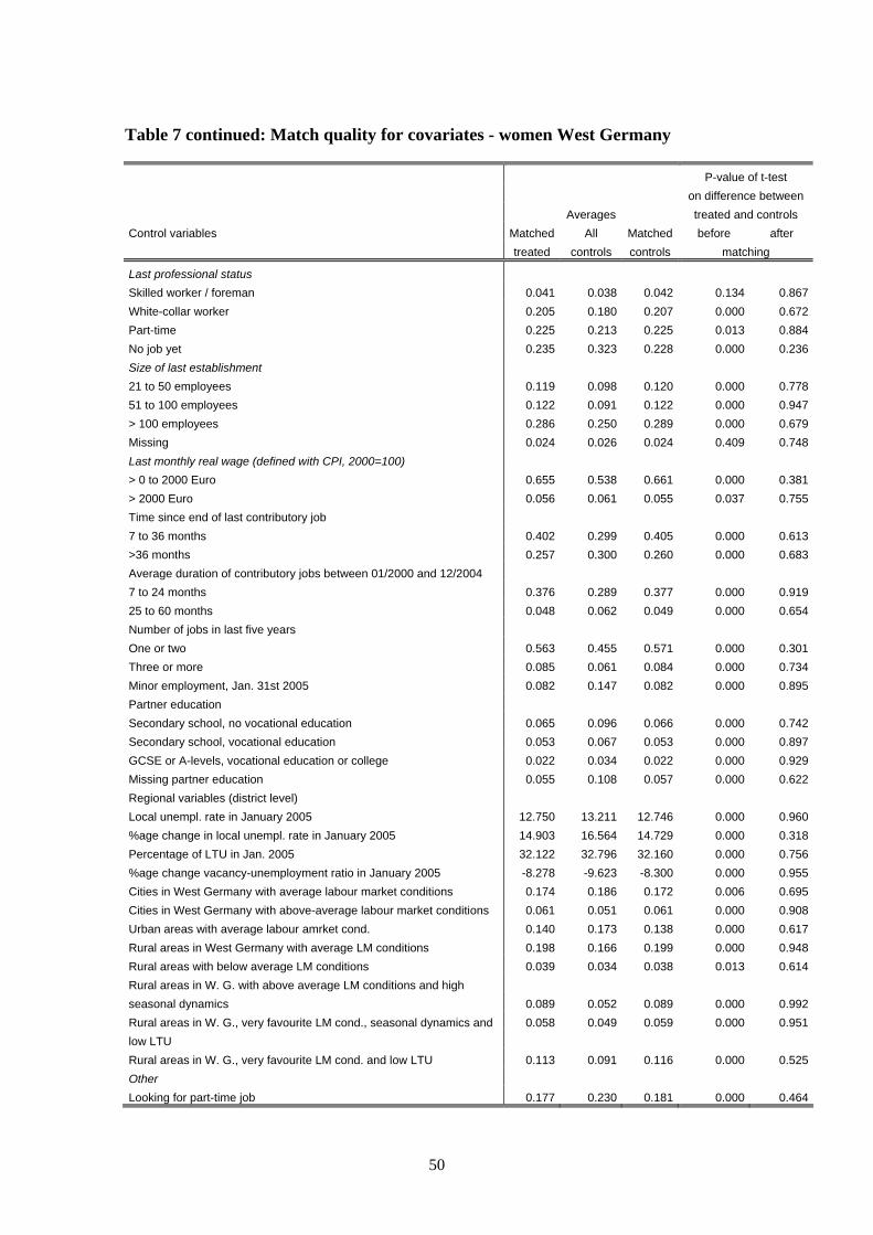
50

Table 7 continued: Match quality for covariates - women West Germany

P-value of t-test on difference between Averages treated and controls Control variables Matched All Matched before after treated controls controls matching

Last professional status Skilled worker / foreman 0.041 0.038 0.042 0.134 0.867White-collar worker 0.205 0.180 0.207 0.000 0.672Part-time 0.225 0.213 0.225 0.013 0.884No job yet 0.235 0.323 0.228 0.000 0.236Size of last establishment 21 to 50 employees 0.119 0.098 0.120 0.000 0.77851 to 100 employees 0.122 0.091 0.122 0.000 0.947> 100 employees 0.286 0.250 0.289 0.000 0.679Missing 0.024 0.026 0.024 0.409 0.748Last monthly real wage (defined with CPI, 2000=100) > 0 to 2000 Euro 0.655 0.538 0.661 0.000 0.381> 2000 Euro 0.056 0.061 0.055 0.037 0.755Time since end of last contributory job 7 to 36 months 0.402 0.299 0.405 0.000 0.613>36 months 0.257 0.300 0.260 0.000 0.683Average duration of contributory jobs between 01/2000 and 12/2004 7 to 24 months 0.376 0.289 0.377 0.000 0.91925 to 60 months 0.048 0.062 0.049 0.000 0.654Number of jobs in last five years One or two 0.563 0.455 0.571 0.000 0.301Three or more 0.085 0.061 0.084 0.000 0.734Minor employment, Jan. 31st 2005 0.082 0.147 0.082 0.000 0.895Partner education Secondary school, no vocational education 0.065 0.096 0.066 0.000 0.742Secondary school, vocational education 0.053 0.067 0.053 0.000 0.897GCSE or A-levels, vocational education or college 0.022 0.034 0.022 0.000 0.929Missing partner education 0.055 0.108 0.057 0.000 0.622Regional variables (district level) Local unempl. rate in January 2005 12.750 13.211 12.746 0.000 0.960%age change in local unempl. rate in January 2005 14.903 16.564 14.729 0.000 0.318Percentage of LTU in Jan. 2005 32.122 32.796 32.160 0.000 0.756%age change vacancy-unemployment ratio in January 2005 -8.278 -9.623 -8.300 0.000 0.955Cities in West Germany with average labour market conditions 0.174 0.186 0.172 0.006 0.695Cities in West Germany with above-average labour market conditions 0.061 0.051 0.061 0.000 0.908Urban areas with average labour amrket cond. 0.140 0.173 0.138 0.000 0.617Rural areas in West Germany with average LM conditions 0.198 0.166 0.199 0.000 0.948Rural areas with below average LM conditions 0.039 0.034 0.038 0.013 0.614Rural areas in W. G. with above average LM conditions and high seasonal dynamics 0.089 0.052 0.089 0.000 0.992Rural areas in W. G., very favourite LM cond., seasonal dynamics and 0.058 0.049 0.059 0.000 0.951low LTU Rural areas in W. G., very favourite LM cond. and low LTU 0.113 0.091 0.116 0.000 0.525Other Looking for part-time job 0.177 0.230 0.181 0.000 0.464

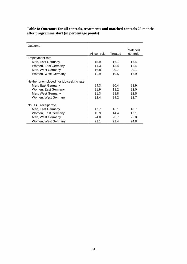
51

Table 8: Outcomes for all controls, treatments and matched controls 20 months after programme start (in percentage points)

Outcome

All controls Treated Matched controls

Employment rate Men, East Germany 15.9 16.1 16.4 Women, East Germany 11.3 13.4 12.4 Men, West Germany 16.8 20.7 20.1 Women, West Germany 12.9 19.5 16.9 Neither unemployed nor job-seeking rate Men, East Germany 24.3 20.4 23.9 Women, East Germany 21.9 18.2 22.0 Men, West Germany 31.3 28.8 32.5 Women, West Germany 32.4 29.2 32.7 No UB II receipt rate Men, East Germany 17.7 16.1 18.7 Women, East Germany 15.9 14.4 17.1 Men, West Germany 24.0 23.7 26.8 Women, West Germany 22.1 22.4 24.8

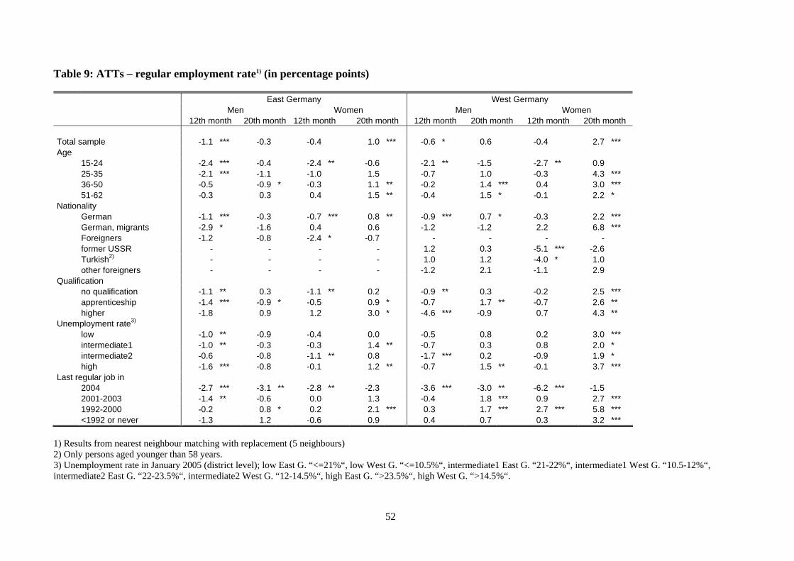
52

Table 9: ATTs – regular employment rate1) (in percentage points)

East Germany West Germany Men Women Men Women 12th month 20th month 12th month 20th month 12th month 20th month 12th month 20th month Total sample -1.1 *** -0.3 -0.4 1.0 *** -0.6 * 0.6 -0.4 2.7 *** Age 15-24 -2.4 *** -0.4 -2.4 ** -0.6 -2.1 ** -1.5 -2.7 ** 0.9 25-35 -2.1 *** -1.1 -1.0 1.5 -0.7 1.0 -0.3 4.3 *** 36-50 -0.5 -0.9 * -0.3 1.1 ** -0.2 1.4 *** 0.4 3.0 *** 51-62 -0.3 0.3 0.4 1.5 ** -0.4 1.5 * -0.1 2.2 * Nationality German -1.1 *** -0.3 -0.7 *** 0.8 ** -0.9 *** 0.7 * -0.3 2.2 *** German, migrants -2.9 * -1.6 0.4 0.6 -1.2 -1.2 2.2 6.8 *** Foreigners -1.2 -0.8 -2.4 * -0.7 - - - - former USSR - - - - 1.2 0.3 -5.1 *** -2.6 Turkish2) - - - - 1.0 1.2 -4.0 * 1.0 other foreigners - - - - -1.2 2.1 -1.1 2.9 Qualification no qualification -1.1 ** 0.3 -1.1 ** 0.2 -0.9 ** 0.3 -0.2 2.5 *** apprenticeship -1.4 *** -0.9 * -0.5 0.9 * -0.7 1.7 ** -0.7 2.6 ** higher -1.8 0.9 1.2 3.0 * -4.6 *** -0.9 0.7 4.3 ** Unemployment rate3) low -1.0 ** -0.9 -0.4 0.0 -0.5 0.8 0.2 3.0 *** intermediate1 -1.0 ** -0.3 -0.3 1.4 ** -0.7 0.3 0.8 2.0 * intermediate2 -0.6 -0.8 -1.1 ** 0.8 -1.7 *** 0.2 -0.9 1.9 * high -1.6 *** -0.8 -0.1 1.2 ** -0.7 1.5 ** -0.1 3.7 *** Last regular job in 2004 -2.7 *** -3.1 ** -2.8 ** -2.3 -3.6 *** -3.0 ** -6.2 *** -1.5 2001-2003 -1.4 ** -0.6 0.0 1.3 -0.4 1.8 *** 0.9 2.7 *** 1992-2000 -0.2 0.8 * 0.2 2.1 *** 0.3 1.7 *** 2.7 *** 5.8 *** <1992 or never -1.3 1.2 -0.6 0.9 0.4 0.7 0.3 3.2 ***

1) Results from nearest neighbour matching with replacement (5 neighbours) 2) Only persons aged younger than 58 years. 3) Unemployment rate in January 2005 (district level); low East G. “<=21%“, low West G. “<=10.5%“, intermediate1 East G. “21-22%“, intermediate1 West G. “10.5-12%“, intermediate2 East G. “22-23.5%“, intermediate2 West G. “12-14.5%“, high East G. “>23.5%“, high West G. “>14.5%“.

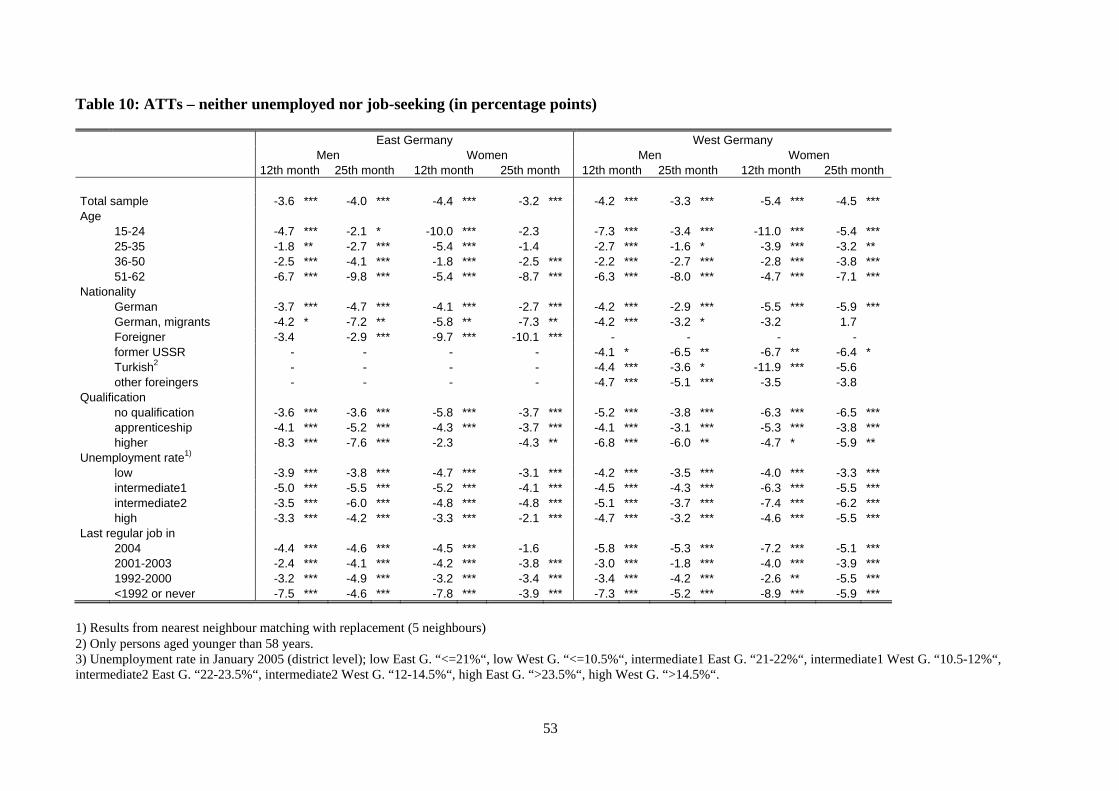
53

Table 10: ATTs – neither unemployed nor job-seeking (in percentage points)

East Germany West Germany Men Women Men Women 12th month 25th month 12th month 25th month 12th month 25th month 12th month 25th month Total sample -3.6 *** -4.0 *** -4.4 *** -3.2 *** -4.2 *** -3.3 *** -5.4 *** -4.5 *** Age 15-24 -4.7 *** -2.1 * -10.0 *** -2.3 -7.3 *** -3.4 *** -11.0 *** -5.4 *** 25-35 -1.8 ** -2.7 *** -5.4 *** -1.4 -2.7 *** -1.6 * -3.9 *** -3.2 ** 36-50 -2.5 *** -4.1 *** -1.8 *** -2.5 *** -2.2 *** -2.7 *** -2.8 *** -3.8 *** 51-62 -6.7 *** -9.8 *** -5.4 *** -8.7 *** -6.3 *** -8.0 *** -4.7 *** -7.1 *** Nationality German -3.7 *** -4.7 *** -4.1 *** -2.7 *** -4.2 *** -2.9 *** -5.5 *** -5.9 *** German, migrants -4.2 * -7.2 ** -5.8 ** -7.3 ** -4.2 *** -3.2 * -3.2 1.7 Foreigner -3.4 -2.9 *** -9.7 *** -10.1 *** - - - - former USSR - - - - -4.1 * -6.5 ** -6.7 ** -6.4 * Turkish2 - - - - -4.4 *** -3.6 * -11.9 *** -5.6 other foreingers - - - - -4.7 *** -5.1 *** -3.5 -3.8 Qualification no qualification -3.6 *** -3.6 *** -5.8 *** -3.7 *** -5.2 *** -3.8 *** -6.3 *** -6.5 *** apprenticeship -4.1 *** -5.2 *** -4.3 *** -3.7 *** -4.1 *** -3.1 *** -5.3 *** -3.8 *** higher -8.3 *** -7.6 *** -2.3 -4.3 ** -6.8 *** -6.0 ** -4.7 * -5.9 ** Unemployment rate1) low -3.9 *** -3.8 *** -4.7 *** -3.1 *** -4.2 *** -3.5 *** -4.0 *** -3.3 *** intermediate1 -5.0 *** -5.5 *** -5.2 *** -4.1 *** -4.5 *** -4.3 *** -6.3 *** -5.5 *** intermediate2 -3.5 *** -6.0 *** -4.8 *** -4.8 *** -5.1 *** -3.7 *** -7.4 *** -6.2 *** high -3.3 *** -4.2 *** -3.3 *** -2.1 *** -4.7 *** -3.2 *** -4.6 *** -5.5 *** Last regular job in 2004 -4.4 *** -4.6 *** -4.5 *** -1.6 -5.8 *** -5.3 *** -7.2 *** -5.1 *** 2001-2003 -2.4 *** -4.1 *** -4.2 *** -3.8 *** -3.0 *** -1.8 *** -4.0 *** -3.9 *** 1992-2000 -3.2 *** -4.9 *** -3.2 *** -3.4 *** -3.4 *** -4.2 *** -2.6 ** -5.5 *** <1992 or never -7.5 *** -4.6 *** -7.8 *** -3.9 *** -7.3 *** -5.2 *** -8.9 *** -5.9 ***

1) Results from nearest neighbour matching with replacement (5 neighbours) 2) Only persons aged younger than 58 years. 3) Unemployment rate in January 2005 (district level); low East G. “<=21%“, low West G. “<=10.5%“, intermediate1 East G. “21-22%“, intermediate1 West G. “10.5-12%“, intermediate2 East G. “22-23.5%“, intermediate2 West G. “12-14.5%“, high East G. “>23.5%“, high West G. “>14.5%“.

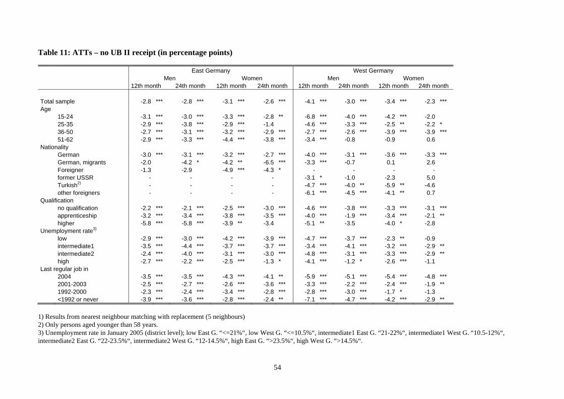
54

Table 11: ATTs – no UB II receipt (in percentage points)

East Germany West Germany Men Women Men Women 12th month 24th month 12th month 24th month 12th month 24th month 12th month 24th month Total sample -2.8 *** -2.8 *** -3.1 *** -2.6 *** -4.1 *** -3.0 *** -3.4 *** -2.3 *** Age 15-24 -3.1 *** -3.0 *** -3.3 *** -2.8 ** -6.8 *** -4.0 *** -4.2 *** -2.0 25-35 -2.9 *** -3.8 *** -2.9 *** -1.4 -4.6 *** -3.3 *** -2.5 ** -2.2 * 36-50 -2.7 *** -3.1 *** -3.2 *** -2.9 *** -2.7 *** -2.6 *** -3.9 *** -3.9 *** 51-62 -2.9 *** -3.3 *** -4.4 *** -3.8 *** -3.4 *** -0.8 -0.9 0.6 Nationality German -3.0 *** -3.1 *** -3.2 *** -2.7 *** -4.0 *** -3.1 *** -3.6 *** -3.3 *** German, migrants -2.0 -4.2 * -4.2 ** -6.5 *** -3.3 *** -0.7 0.1 2.6 Foreigner -1.3 -2.9 -4.9 *** -4.3 * - - - - former USSR - - - - -3.1 * -1.0 -2.3 5.0 Turkish2) - - - - -4.7 *** -4.0 ** -5.9 ** -4.6 other foreigners - - - - -6.1 *** -4.5 *** -4.1 ** 0.7 Qualification no qualification -2.2 *** -2.1 *** -2.5 *** -3.0 *** -4.6 *** -3.8 *** -3.3 *** -3.1 *** apprenticeship -3.2 *** -3.4 *** -3.8 *** -3.5 *** -4.0 *** -1.9 *** -3.4 *** -2.1 ** higher -5.8 *** -5.8 *** -3.9 ** -3.4 -5.1 ** -3.5 -4.0 * -2.8 Unemployment rate3) low -2.9 *** -3.0 *** -4.2 *** -3.9 *** -4.7 *** -3.7 *** -2.3 ** -0.9 intermediate1 -3.5 *** -4.4 *** -3.7 *** -3.7 *** -3.4 *** -4.1 *** -3.2 *** -2.9 ** intermediate2 -2.4 *** -4.0 *** -3.1 *** -3.0 *** -4.8 *** -3.1 *** -3.3 *** -2.9 ** high -2.7 *** -2.2 *** -2.5 *** -1.3 * -4.1 *** -1.2 * -2.6 *** -1.1 Last regular job in 2004 -3.5 *** -3.5 *** -4.3 *** -4.1 ** -5.9 *** -5.1 *** -5.4 *** -4.8 *** 2001-2003 -2.5 *** -2.7 *** -2.6 *** -3.6 *** -3.3 *** -2.2 *** -2.4 *** -1.9 ** 1992-2000 -2.3 *** -2.4 *** -3.4 *** -2.8 *** -2.8 *** -3.0 *** -1.7 * -1.3 <1992 or never -3.9 *** -3.6 *** -2.8 *** -2.4 ** -7.1 *** -4.7 *** -4.2 *** -2.9 **

1) Results from nearest neighbour matching with replacement (5 neighbours) 2) Only persons aged younger than 58 years. 3) Unemployment rate in January 2005 (district level); low East G. “<=21%“, low West G. “<=10.5%“, intermediate1 East G. “21-22%“, intermediate1 West G. “10.5-12%“, intermediate2 East G. “22-23.5%“, intermediate2 West G. “12-14.5%“, high East G. “>23.5%“, high West G. “>14.5%“.

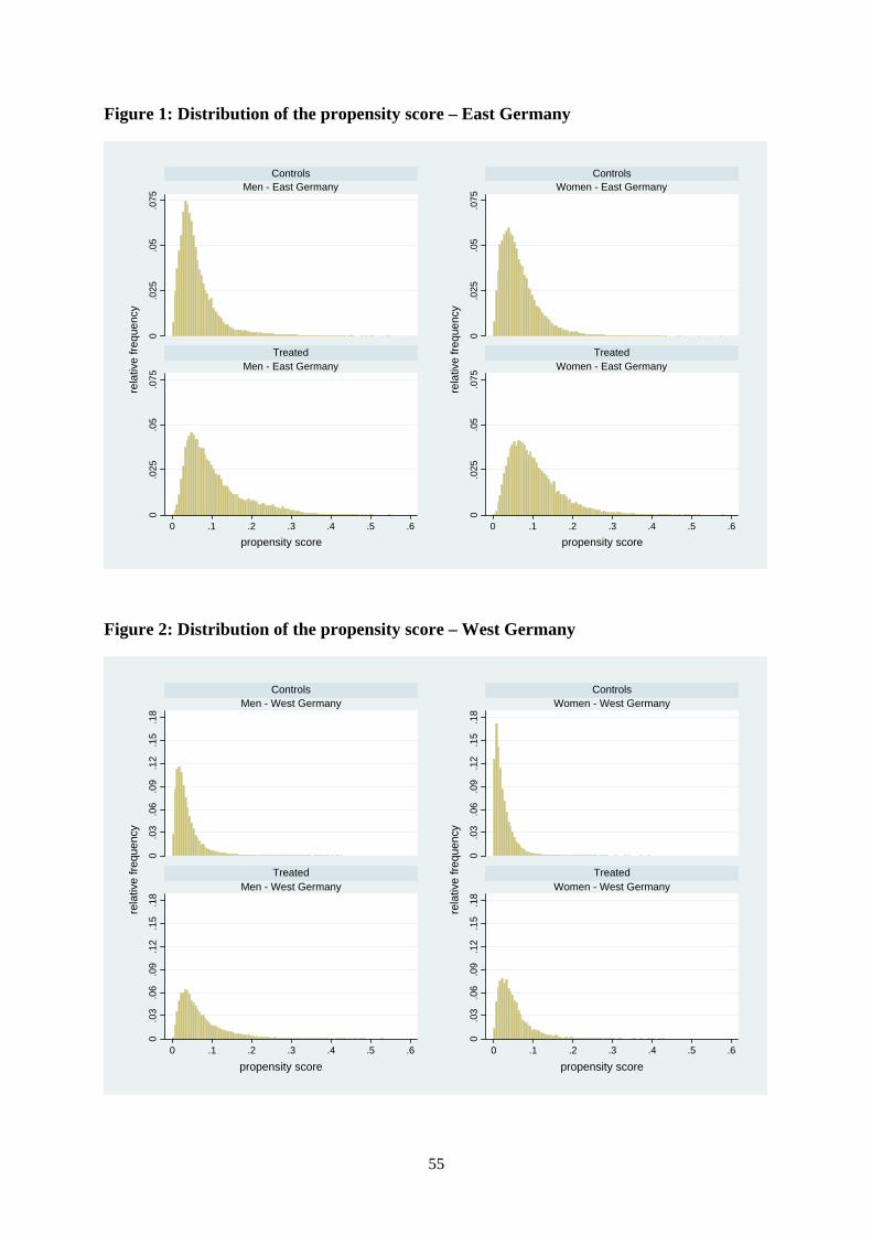
55

Figure 1: Distribution of the propensity score – East Germany

0.0

25.0

5.0

750

.025

.05

.075

0 .1 .2 .3 .4 .5 .6

Men - East Germany

Men - East Germany

Controls

Treated

rela

tive

frequ

ency

propensity score

0.0

25.0

5.0

750

.025

.05

.075

0 .1 .2 .3 .4 .5 .6

Women - East Germany

Women - East Germany

Controls

Treated

rela

tive

frequ

ency

propensity score

Figure 2: Distribution of the propensity score – West Germany

0.0

3.0

6.0

9.1

2.1

5.1

80

.03

.06

.09

.12

.15

.18

0 .1 .2 .3 .4 .5 .6

Men - West Germany

Men - West Germany

Controls

Treated

rela

tive

frequ

ency

propensity score

0.0

3.0

6.0

9.1

2.1

5.1

80

.03

.06

.09

.12

.15

.18

0 .1 .2 .3 .4 .5 .6

Women - West Germany

Women - West Germany

Controls

Treated

rela

tive

frequ

ency

propensity score

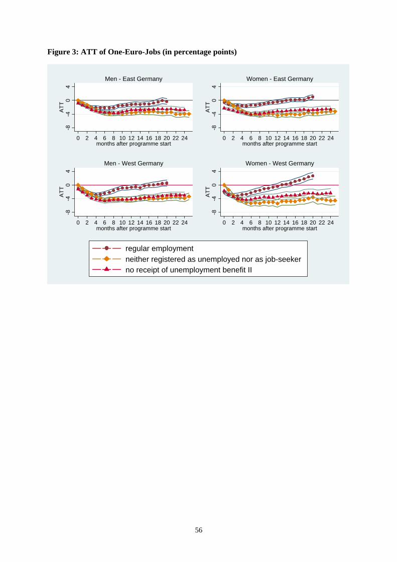
56

Figure 3: ATT of One-Euro-Jobs (in percentage points)

-8-4

04

ATT

0 2 4 6 8 10 12 14 16 18 20 22 24months after programme start

Men - East Germany

-8-4

04

ATT

0 2 4 6 8 10 12 14 16 18 20 22 24months after programme start

Women - East Germany

-8-4

04

ATT

0 2 4 6 8 10 12 14 16 18 20 22 24months after programme start

Men - West Germany

-8-4

04

ATT

0 2 4 6 8 10 12 14 16 18 20 22 24months after programme start

Women - West Germany

regular employmentneither registered as unemployed nor as job-seekerno receipt of unemployment benefit II