Embed Size (px)
Citation preview
A First Course in ClimateEarth and Elsewhere
Volume I: Thermodynamics and radiationVolume II: Dynamics of the Atmosphere
(with just enough oceanography to get by)
R. T. PierrehumbertDepartment of Geophysical Sciences
University of ChicagoChicago, IL
2 A First Course in Climate
Preface[**Course from standpoint of somebody who comes in from outside. My
experience on moving to U. of. C. Envious of colleagues working on sweeping problems
like Cretaceous warmth. What's a poor dynamicist to do? For that matter, what's a poor
paleoclimatologist to do? (to get background in the necessary climate physics).]
[** "Just enough." i.e. just enough radiation, just enough thermodynamics, etc.]
[**Interweave data, theory and models. Include source code and data for just about
everything used in book, on accompanying CD-ROM.]
3 A First Course in Climate
1. Introduction – The Big QuestionsCentral (to us!): Robust equable climate of earth (all three phases of water co-
exist). Has been like this for about 3. billion years, despite massive changes in continents,
atmospheric composition and solar output. Below we will give an overview of some of the
major outstanding problems for climate theory.
The Faint Young Sun
History of presumed solar output, and reasons (NB. recent speculations about early
solar mass loss). Implies ice-covered, and perhaps ice-locked early earth (will go into ice-
albedo feedback in more detail later in the course. Evidence for liquid water in Archaean
and PreCambrian times. Many impacts 4.2-3.9Ga, may have brought oceans to boiling;
high temperature crust, temperatures as high as 1200C. Crustal formation 3.8-4Ga.
Microcontinents 3.8-2.5Ga, but large continents after 2.5Ga. Banded iron 2.5-2Ga,
indicating oxygen and photosynthesis; expansion of blue-green algae (stromatolites --
carbonate evidence). In fact, earliest stromatolites are found 3.3-3.5Ga, and are coeval with
the first carbonates (formed by weathering, and indicative of removal of CO2 from
atmosphere). Note life didn't have much time to get started! Life implies liquid water.
Oldest glacial rocks are 2.7Ga. [**NB: for classes where some students have familiarity
with energy balance models, use this as a vehicle for reviewing the material. Ignore
atmosphere.]
Warm climate ages
Present kind of climate has cold ice-covered poles. Much of Earth History, have
had warm, ice-free climates (or perhaps only seasonal ice). Formerly thought that these
climates represented 90% of record, but re-examination of evidence, esp. last 100Myr, has
thrown this into doubt. Early warm climates: Ice free earth from 4.6 to 2.5 Ga, and from
2.5 - .9 Ga despite faint sun. (But how good is evidence? Mostly comes from lack of
certain ice-related deposits. Note, though, evidence that at least some liquid water existed
throughout this time is quite firm.) Also generally mild from .6 to .1Ga. Note esp. mid-
cretaceous (100Ma) and eocene (55Ma). Strong evidence that there was little or no
permanent polar ice in the mid-Cretatious, though surface temperature estimates somewhat
uncertain; not clear whether tropics was warmer than now. Dinosaurs up to Arctic circle.
Eocene warm climate is the best documented. During eocene, tropics were about as warm
as now, but poles were believed to be 10-150C warmer, and also without much of a
4 A First Course in Climate
winter. Alligators and lemurs as far north as 78o. Problem: How to warm up poles
without warming up tropics?
Glaciation
From time to time, factors maintaining warm climates break down. First glaciation
about 2.5Ga. Pre-cambrian glaciation: 3 major glaciations between .9 to .6 Ga.
Particularly interesting because of evidence of ice even in paleo-tropics. The generally mild
climate from .6 to .1Ga, had 2 major glaciations: Late Ordovician ca 440Ma and Permian,
ca 280-225 Ma (length not well fixed), but there may also have been more seasonal ice
than previously thought. Cooling between 50 and 3 Ma, leading into the present glacial
era.
Effect of Bolide impact
Dust veil. Evaporation of water? Note esp. mass extinctions at KT boundary.
Similar problems for major volcanic eruption eras. Possible future applications — what
happens if Swift/Tuttle or something similar hits us?
Pleistocene ice ages
During the past 2M years, have good time resolution on fluctuations in extent of
glaciers. During the whole time, there has been ice at the poles, but the ice-sheet has
repetitively advanced and retreated. δO18 record (ice volume effect vs. sea surface
temperature). Dominant period is 100Kyr, recently, but earlier was more like 40Kyr.
Where we are now: just past the "climatic optimum" following previous ice age. Details of
temperature and glacial extent over past 20Kyr. Problem of rapid deglaciation.
Comparative Climatology
Earth-Mars-Venus divergent climate evolution. Loss of water from atmosphere to
space. Loss of other atmospheric constituents. "Water vapor traps?" Iceteroids? Evidence
for early water & warm climate on Mars.
Planetary circulation patterns & jet structure. Venus, Earth, Mars, Jupiter, Saturn,
Uranus & Neptune. Multiple jets and persistent eddies on the giant planets. Note that the
most weakly thermally driven planets (Neptune, Uranus) have the strongest winds. Why?
Basic problems in present climates
Vertical structure of atmospheres: Troposphere & stratosphere, tropospheric lapse
rate. Why is atmosphere stably stratified at all? Solar radiation heats atmosphere from
below; why don't we get a "stellar type" convective circulation. [**NB for students that
5 A First Course in Climate
know basic atmospheric thermodynamics, use this as a vehicle for reviewing potential
temperature and hydrostatic balance. This topic should perhaps be moved to next section.]
Determination of pole-equator temperature gradients (NB: Venus has essentially no
P-E gradient), and meridonal heat fluxes in atmospheres and oceans.
Amplitude of the seasonal cycle. Seasonal cycle of lapse rate (will be interesting to
compare with Mars!)
Determination of how much incident sunlight the Earth reflects; role of clouds.
Moisture distribution in the Earth's atmosphere. Note radiative importance of water
vapor, esp. mid-tropospheric water vapor.
Note: The currently important issue of human-induced "greenhouse warming"
represent small effects in the grand scheme of things (2-4oK averaged over the globe and
over the year.), which is why they are hard to predict precisely. But note also: Crowley
points out that the combination of glaciated poles and warm extratropics may be unique in
Earth history.
[**Pick out some of the above issues (e.g. faint young sun, CO2 needed for
martian water), and keep coming back to it more and more quantitatively as the necessary
tools are developed.]
6 A First Course in Climate
2. Vertical structure of compressible atmospheresor, "All the thermodynamics I need to know, I learned in kindergarten."
The atmospheres which are our principal objects of study are made of compressible
gases. The compressibility has a profound effect on the vertical profile of temperature in
these atmospheres. As things progress it will become clear that the vertical temperature
variation in turn strongly influences the planet's climate. To deal with these effects it will
be necessary to know some thermodynamics — though just a little. This chapter does not
purport to be a complete course in thermodynamics. It can only provide a summary of the
key thermodynamic concepts and formulae needed to treat the basic problems of planetary
climate. It is assumed that the student has obtained (or will obtain) a more fundamental
understanding of the general subject of thermodynamics elsewhere.
2.1 A few observations
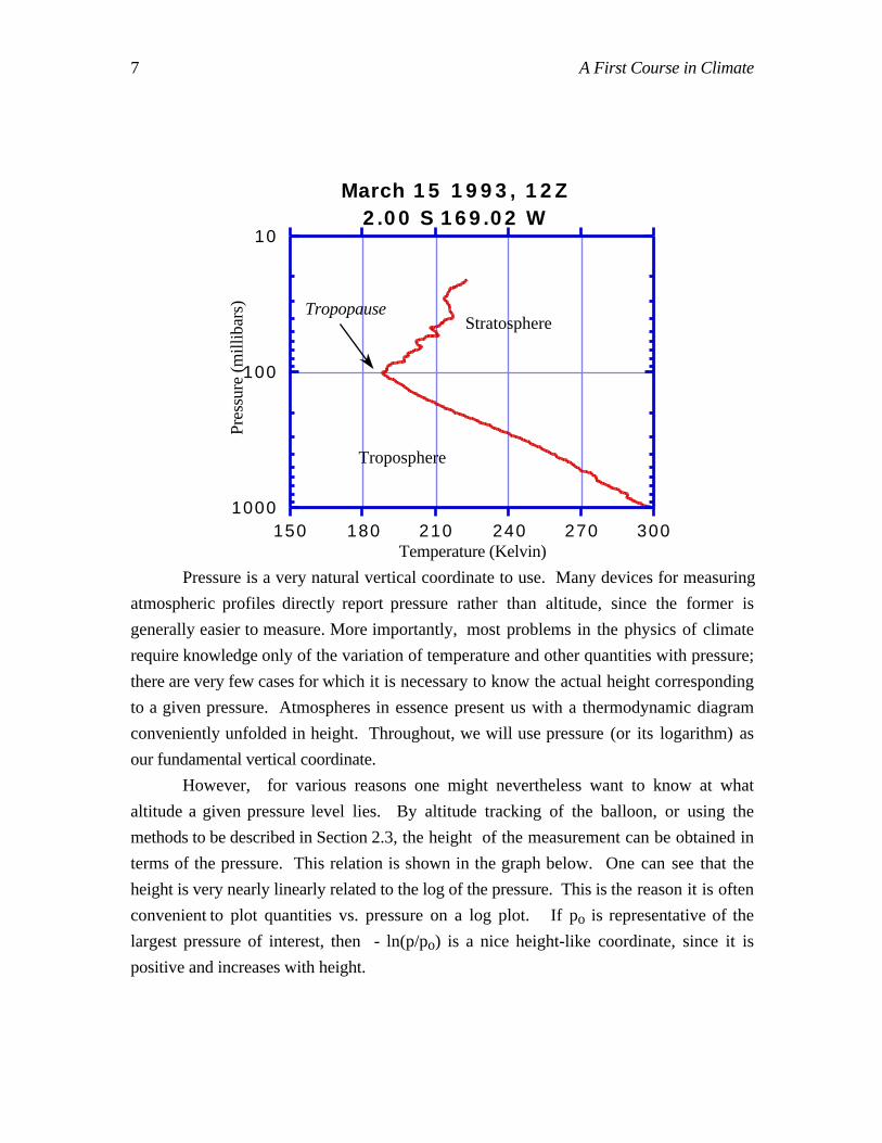
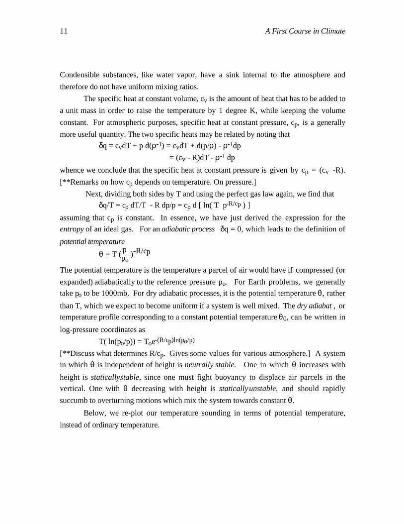
The following temperature profile measured in the Earth's tropics introduces most
of the features that are of interest in the study of general planetary atmospheres. It was
obtained by releasing a "weather balloon" (more properly, a "radiosonde") which floats
upwards from the ground, and radios back data on temperature and pressure as it rises.
Pressure goes down monotonically with height, so the lower pressures represent greater
altitudes.
7 A First Course in Climate
10
100
1000150 180 210 240 270 300
March 15 1993, 12Z2.00 S 169.02 W
Pres
sure
(m
illib
ars)
Temperature (Kelvin)
Tropopause
Troposphere
Stratosphere
Pressure is a very natural vertical coordinate to use. Many devices for measuring
atmospheric profiles directly report pressure rather than altitude, since the former is
generally easier to measure. More importantly, most problems in the physics of climate
require knowledge only of the variation of temperature and other quantities with pressure;
there are very few cases for which it is necessary to know the actual height corresponding
to a given pressure. Atmospheres in essence present us with a thermodynamic diagram
conveniently unfolded in height. Throughout, we will use pressure (or its logarithm) as
our fundamental vertical coordinate.
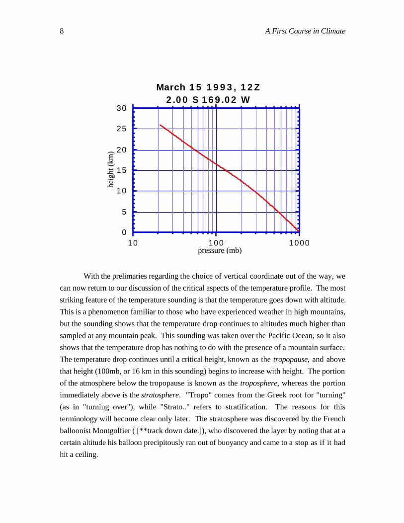
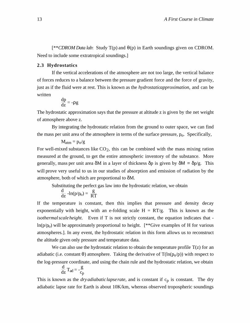
However, for various reasons one might nevertheless want to know at what
altitude a given pressure level lies. By altitude tracking of the balloon, or using the
methods to be described in Section 2.3, the height of the measurement can be obtained in
terms of the pressure. This relation is shown in the graph below. One can see that the
height is very nearly linearly related to the log of the pressure. This is the reason it is often
convenient to plot quantities vs. pressure on a log plot. If po is representative of the
largest pressure of interest, then - ln(p/po) is a nice height-like coordinate, since it is
positive and increases with height.
8 A First Course in Climate
0
5
10
15
20
25
30
10 100 1000
March 15 1993, 12Z2.00 S 169.02 W
heig
ht (
km)
pressure (mb)
With the prelimaries regarding the choice of vertical coordinate out of the way, we
can now return to our discussion of the critical aspects of the temperature profile. The most
striking feature of the temperature sounding is that the temperature goes down with altitude.
This is a phenomenon familiar to those who have experienced weather in high mountains,
but the sounding shows that the temperature drop continues to altitudes much higher than
sampled at any mountain peak. This sounding was taken over the Pacific Ocean, so it also
shows that the temperature drop has nothing to do with the presence of a mountain surface.
The temperature drop continues until a critical height, known as the tropopause, and above
that height (100mb, or 16 km in this sounding) begins to increase with height. The portion
of the atmosphere below the tropopause is known as the troposphere, whereas the portion
immediately above is the stratosphere. "Tropo" comes from the Greek root for "turning"
(as in "turning over"), while "Strato.." refers to stratification. The reasons for this
terminology will become clear only later. The stratosphere was discovered by the French
balloonist Montgolfier ( [**track down date.]), who discovered the layer by noting that at a
certain altitude his balloon precipitously ran out of buoyancy and came to a stop as if it had
hit a ceiling.
9 A First Course in Climate
The sounding we have shown is qualitatively typical, and raises a number of
questions. Why does the temperature decrease with height in the lower layer? Why isn't
the situation with cold air over warm air unstable? Why does the temperature increase with
height in the stratosphere? What determines the tropopause height? How does it vary with
time and position? Providing physically based answers to these questions, for the
atmospheres of Earth and other planets, will be one of our main preoccupations in
subsequent chapters.
[**Add some extratropical soundings, to give an idea of how tropopause varies
with latitude. Do this as a composite page of several tropical and several extratropical
soundings, with extratropical soundings over land and ocean, and at various seasons.]
[**Put in Galileo probe for Jupiter, and some Mars profiles. Phenomena not
specific only to Earth.]
2.2 Dry thermodynamics
The three thermodynamic variables with which we will mainly be concerned are:
temperature (denoted by T), pressure ( denoted by p) and density (denoted by ρ).
Temperature is a measure of the amount of kinetic energy per molecule in the molecules
making up the gas. We will always measure temperature in degrees Kelvin, which are the
same as degrees Celsius (or Centigrade), except offset so that absolute zero — the
temperature at which molecular motion ceases — occurs at zero Kelvin. In Celsius
degrees, absolute zero occurs at about -273.15 C, which is then 0K by definition.
Pressure is a measure of the flux of momentum per unit time carried by the
molecules of the gas passing through an imaginary surface of unit area; equivalently, it is a
measure of the force per unit area exerted on a surface in contact with the gas. In the mks
units we employ throughout this book , pressure is measured in Pascals (Pa); 1 Pascal is 1
kg/(m s). For historical reasons, atmospheric pressures are often measured in "bars" or
"millibars." One bar, or equivalently 1000 millibars (mb) is approximately the mean sea-
level pressure of the Earth's current atmosphere. We will often lapse into using mb as
units of pressure, because the unit sounds comfortable to atmospheric scientists. For
calculations, though, it is important to convert millibars to Pascals. This is easy, because 1
mb = 100 Pa. Hence, we should all learn to say "Hectopascal" in place of "millibar." It
may take some time.
Density is simply the mass of the gas contained in a unit of volume. In mks units,
it is measured in kg/m3.
10 A First Course in Climate
For a perfect gas, the three thermodynamic variables are related by the perfect gas
equation of state, which can be written
p = ρ R*M T
where R* is the universal gas constant, which is independent of the gas in question, and M
is the molecular weight of the gas. We can define the gas constant R = R*/M pertinent to
the gas in question. For example, dry Earth air has a mean molecular weight of 28.97, so
Rdry air = 287, in mks units. Generally speaking, a gas obeys the perfect gas law when it is
tenuous enough that the energy stored in forces between the molecules making up the gas is
negligable. Deviations from the perfect gas law can be very important for the dense
atmosphere of Venus, but for the purposes of the current atmosphere of Earth or Mars, or
the upper part of the Jovian atmosphere, the perfect gas law can be regarded as an accurate
model of the thermodynamics— in fact, "perfect," one might say.
An extension of the concept of a perfect gas is the law of partial pressures. This
states that, in a mixture of gases in a given volume, each component gas behaves just as it
would if it occupied the volume alone. The pressure due to one component gas is called the
partial pressure of that gas. For a mixture of air and CO2, for example, the partial
pressures of the two gases are
pCO2 = RCO2 ρCO2T
pair = Rair ρair T
where the two temperatures are taken to be identical, in accordance with thermodynamic
equilibrium. Concentrations of atmospheric gases are often quoted in terms of ratios of
partial pressure, and are referred to as "volumetric concentration." Thus, when it is said
that the concentration of CO2 in present Earth air is 330 ppmv (parts per million volume),
what is meant is that pCO2/pair = 330 10 -6. The terminology has to do with the fact that a
given number of molecules of any gas always occupies the same volume at a standard
temperature and pressure. If we want to convert to the mass mixing ratio ρCO2/ρair, we
simply take the ratio of the two gas laws, obtaining
ρCO2/ρair = (MCO2/Mair) (pCO2/pair )
in which we have used the definition of the gas constants in terms of the universal gas
constant. It is useful to keep in mind that there is enough atmospheric mixing to keep the
mixing ratio of noncondensible components independent of height up to a great height in
the atmosphere of Earth and other planets. This near-constancy applies in the stratosphere
as well as the troposphere, and holds up to the homopause ( about **km on Earth).
11 A First Course in Climate
Condensible substances, like water vapor, have a sink internal to the atmosphere and
therefore do not have uniform mixing ratios.
The specific heat at constant volume, cv is the amount of heat that has to be added to
a unit mass in order to raise the temperature by 1 degree K, while keeping the volume
constant. For atmospheric purposes, specific heat at constant pressure, cp, is a generally
more useful quantity. The two specific heats may be related by noting that
δq = cvdT + p d(ρ-1) = cvdT + d(p/ρ) - ρ-1dp
= (cv - R)dT - ρ-1 dp
whence we conclude that the specific heat at constant pressure is given by cp = (cv -R).
[**Remarks on how cp depends on temperature. On pressure.]
Next, dividing both sides by T and using the perfect gas law again, we find that
δq/T = cp dT/T - R dp/p = cp d [ ln( T p-R/cp ) ]
assuming that cp is constant. In essence, we have just derived the expression for the
entropy of an ideal gas. For an adiabatic process δq = 0, which leads to the definition of
potential temperature
θ = T (ppo
)-R/cp
The potential temperature is the temperature a parcel of air would have if compressed (or
expanded) adiabatically to the reference pressure po. For Earth problems, we generally
take po to be 1000mb. For dry adiabatic processes, it is the potential temperature θ, rather
than T, which we expect to become uniform if a system is well mixed. The dry adiabat , or
temperature profile corresponding to a constant potential temperature θ0, can be written in
log-pressure coordinates as
T( ln(po/p)) = Toe-(R/cp)ln(po/p)
[**Discuss what determines R/cp. Gives some values for various atmosphere.] A system
in which θ is independent of height is neutrally stable. One in which θ increases with
height is statically stable, since one must fight buoyancy to displace air parcels in the
vertical. One with θ decreasing with height is statically unstable, and should rapidly
succumb to overturning motions which mix the system towards constant θ.
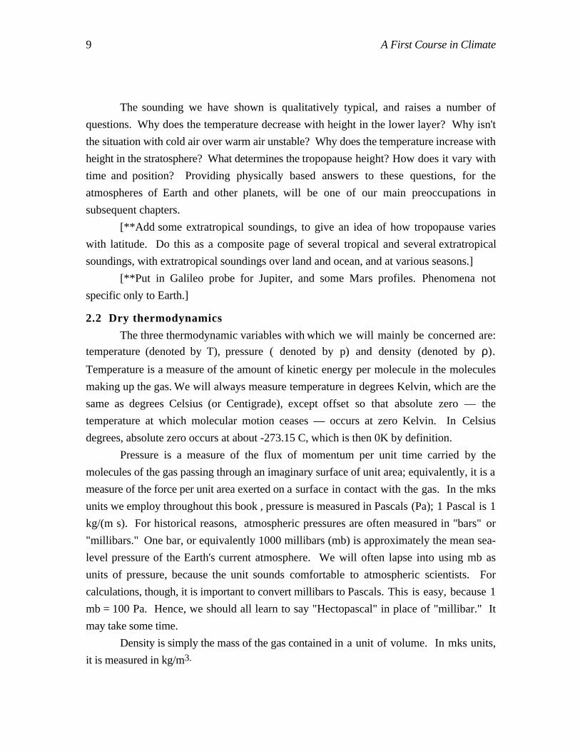
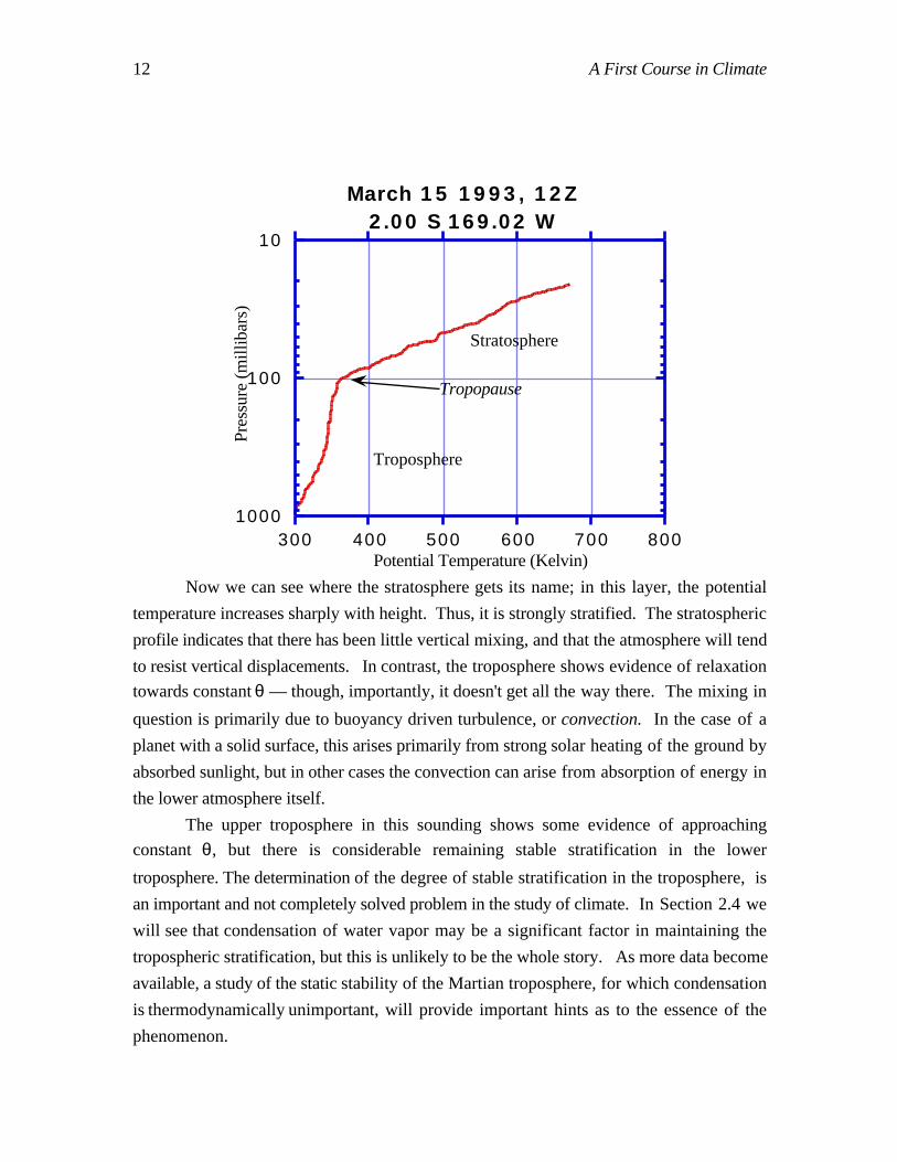
Below, we re-plot our temperature sounding in terms of potential temperature,
instead of ordinary temperature.
12 A First Course in Climate
10
100
1000300 400 500 600 700 800
March 15 1993, 12Z2.00 S 169.02 W
Pres
sure
(m
illib
ars)
Potential Temperature (Kelvin)
Tropopause
Troposphere
Stratosphere
Now we can see where the stratosphere gets its name; in this layer, the potential
temperature increases sharply with height. Thus, it is strongly stratified. The stratospheric
profile indicates that there has been little vertical mixing, and that the atmosphere will tend
to resist vertical displacements. In contrast, the troposphere shows evidence of relaxation
towards constant θ — though, importantly, it doesn't get all the way there. The mixing in
question is primarily due to buoyancy driven turbulence, or convection. In the case of a
planet with a solid surface, this arises primarily from strong solar heating of the ground by
absorbed sunlight, but in other cases the convection can arise from absorption of energy in
the lower atmosphere itself.
The upper troposphere in this sounding shows some evidence of approaching
constant θ, but there is considerable remaining stable stratification in the lower
troposphere. The determination of the degree of stable stratification in the troposphere, is
an important and not completely solved problem in the study of climate. In Section 2.4 we
will see that condensation of water vapor may be a significant factor in maintaining the
tropospheric stratification, but this is unlikely to be the whole story. As more data become
available, a study of the static stability of the Martian troposphere, for which condensation
is thermodynamically unimportant, will provide important hints as to the essence of the
phenomenon.
13 A First Course in Climate
[**CDROM Data lab: Study T(p) and θ(p) in Earth soundings given on CDROM.
Need to include some extratropical soundings.]
2.3 Hydrostatics
If the vertical accelerations of the atmosphere are not too large, the vertical balance
of forces reduces to a balance between the pressure gradient force and the force of gravity,
just as if the fluid were at rest. This is known as the hydrostatic approximation, and can be
writtendpdz = -ρg
The hydrostatic approximation says that the pressure at altitude z is given by the net weight
of atmosphere above z.
By integrating the hydrostatic relation from the ground to outer space, we can find
the mass per unit area of the atmosphere in terms of the surface pressure, po. Specifically,
Matm = po/g
For well-mixed substances like CO2, this can be combined with the mass mixing ration
measured at the ground, to get the entire atmospheric inventory of the substance. More
generally, mass per unit area δM in a layer of thickness δp is given by δΜ = δp/g. This
will prove very useful to us in our studies of absorption and emission of radiation by the
atmosphere, both of which are proportional to δM.
Substituting the perfect gas law into the hydrostatic relation, we obtaind dz -ln(p/po) =
gRT
If the temperature is constant, then this implies that pressure and density decay
exponentially with height, with an e-folding scale H = RT/g. This is known as the
isothermal scale height. Even if T is not strictly constant, the equation indicates that -
ln(p/po) will be approximately proportional to height. [**Give examples of H for various
atmospheres.]. In any event, the hydrostatic relation in this form allows us to reconstruct
the altitude given only pressure and temperature data.
We can also use the hydrostatic relation to obtain the temperature profile T(z) for an
adiabatic (i.e. constant θ) atmosphere. Taking the derivative of T(ln(po/p)) with respect to
the log-pressure coordinate, and using the chain rule and the hydrostatic relation, we obtainddz Tad = -
gcp
This is known as the dry adiabatic lapse rate, and is constant if cp is constant. The dry
adiabatic lapse rate for Earth is about 10K/km, whereas observed tropospheric soundings
14 A First Course in Climate
typically have a lapse rate closer to 6.7K/km. This is just another way of saying that the
troposphere has some residual static stability.
[**Dry static energy. Derivation from expression for δq, using hydrostatic relation
to change dp to dz. Integration in case of constant cp.]
[**Static stability, Brunt-Vaisala frequency.]
2.4 Moist thermodynamics
Many planetary atmospheres have a component that undergoes a phase change from
gaseous to solid or liquid form at some places and times. This is the case for water vapor
on Earth. It also occurs for carbon dioxide on Mars, for methane on Titan, and for
ammonia, water and a few other substances on Jupiter and Saturn. [**Nitrogen
condensation on Triton.]. The influence of condensation on atmospheric structure can be
very important. Therefore, we need to know how to handle the thermodynamics of
systems containing a component that undergoes a phase change. By analogy with water
vapor, the familiar condensible substance on Earth, we shall refer to this subject as "moist
thermodynamics," even though the condensible substance involved is often not water.
The first important concept from moist thermodynamics is latent heat. When a unit
mass of substance at a given temperature undergoes a change to another phase at the same
temperature, a certain amount of energy is released in the transition, owing to differences
amongst the phases in the amount of energy stored in the form of intermolecular
interactions. For example, when one kilogram of water vapor condenses into a liquid, it
releases about 2.5 106 Joules of energy. The amount of energy per unit mass involved in
making the transition from one phase to another (keeping temperature fixed) is known as
the latent heat of the transition. [**Latent heat of fusion. Of vaporization. Of sublimation.
Examples and worked problems.]
The next important concept we take up is that of saturation vapor pressure.
[**Give definition and discuss meaning. Uses definition of partial pressure, if condensible
gas is in a mixture.] Note that condensation is a phase transition problem; the saturation
vapor pressure is just the critical pressure for condensation.
Very general thermodynamic arguments imply that the slope of the saturation vapor
pressure curve ps(T) is given bydpsdT =
1T
L
1/ρv - 1 /ρc
where ρv is the density of the vapor phase and ρc is the density of the condensed phase.
This is the Clausius-Clapeyron equation. Typically, ρv << ρc, so that the second term in
15 A First Course in Climate
the denominator can be neglected. If we further stipulate the perfect gas law for the partial
pressure of the condensing substance, we have 1/ρv = Rv T/ps, soddT ln(ps) =
LRvT2
If, further, L is independent of temperature, we can integrate this relation analytically,
obtaining
ps = p∞ e-L/(RvT)
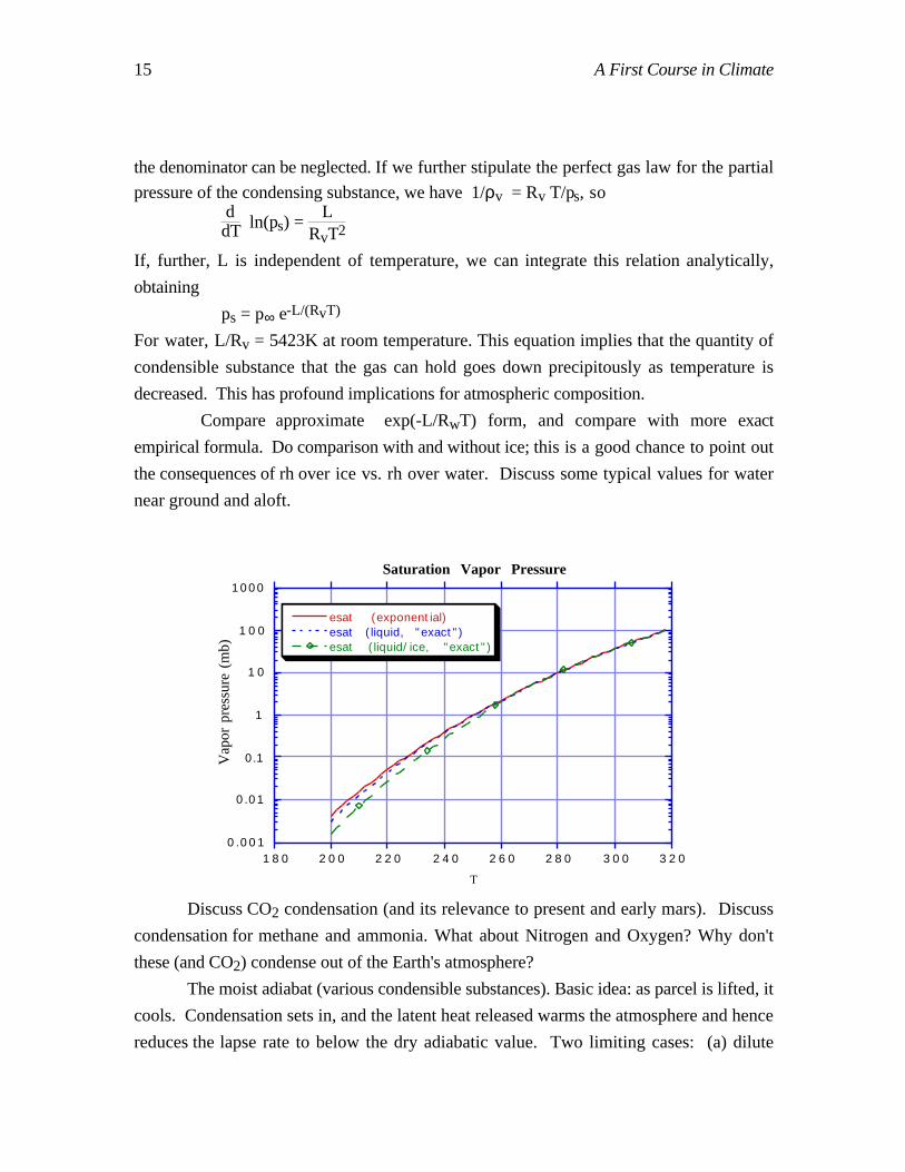
For water, L/Rv = 5423K at room temperature. This equation implies that the quantity of
condensible substance that the gas can hold goes down precipitously as temperature is
decreased. This has profound implications for atmospheric composition.
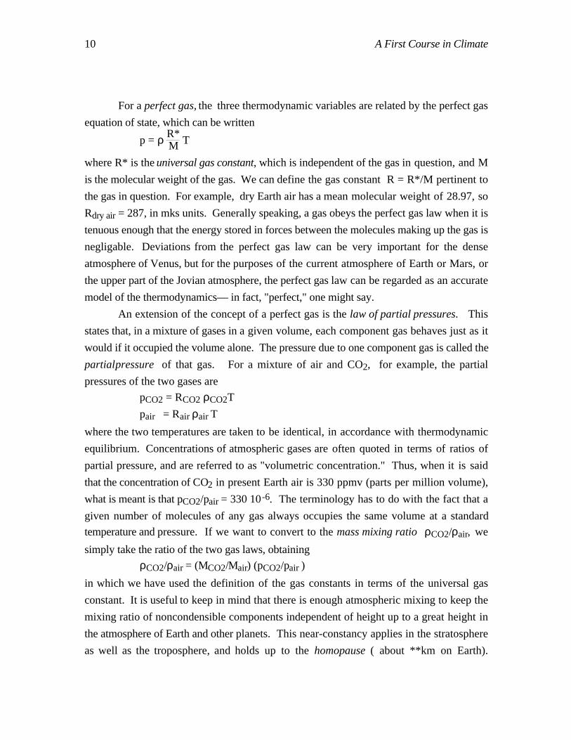
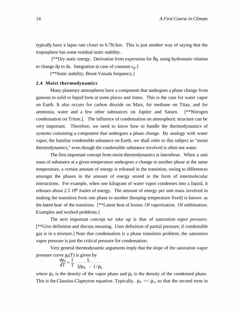
Compare approximate exp(-L/RwT) form, and compare with more exact
empirical formula. Do comparison with and without ice; this is a good chance to point out
the consequences of rh over ice vs. rh over water. Discuss some typical values for water
near ground and aloft.
0.001
0.01
0.1
1
10
100
1000
180 200 220 240 260 280 300 320
Saturation Vapor Pressure
esat (exponential)esat (liquid, "exact")esat (liquid/ice, "exact")
Vap
or p
ress
ure
(mb)
T
Discuss CO2 condensation (and its relevance to present and early mars). Discuss
condensation for methane and ammonia. What about Nitrogen and Oxygen? Why don't
these (and CO2) condense out of the Earth's atmosphere?
The moist adiabat (various condensible substances). Basic idea: as parcel is lifted, it
cools. Condensation sets in, and the latent heat released warms the atmosphere and hence
reduces the lapse rate to below the dry adiabatic value. Two limiting cases: (a) dilute
16 A First Course in Climate
condensible substance, like water vapor on Earth. (b) Case where primary component is
condensible (e.g. CO2 on Mars, or steam in runaway greenhouse atmosphere.). Re-do
atmospheric sounding given above, in terms of θe . Note that most of the Earth's
atmosphere is not undergoing a moist adiabatic process at any given time, so it's not clear
why the moist adiabat should govern the static stability.
17 A First Course in Climate
3. Simple radiation balance models3.1 Elementary properties of radiation
Climate is a problem in the interaction of electromagnetic radiation with matter —
interaction of light from the Sun with matter making up the planet's atmosphere (if it has
one) and surface (if it has one)1. [**We deal largely with something called "blackbody
radiation", which is radiation in thermodynamic equilbrium.] While blackbody radiation
can be conceived of as a gas of photons in thermodynamic equilbrium, characterized by a
temperature T, in normal circumstances photons do not interact with each other strongly
enough to distribute the energy amongst each other and bring the system to equilbrium.
[**think of a gas of photons at T1, another at T2, and mix together. They will just carry
out their ghostly co-existence and never relax toward a single temperature T.] Hence, in
dealing with blackbody radiation, we mostly think of a photon gas in thermodynamic
equilibrium with a blob of matter at temperature T. The absorption and re-emission of
photons by the matter provides the scrambling necessary to maintain equilibrium.
[**Understanding BB radiation is one of the great triumphs of 20th century
physics. See Pais book on Bohr for an intellectual history of the subject. Involves (indeed
led to) quantum theory. In some ways, it was a more important development than
relativity, since the effects of the quantum world are revealed through blackbody radiation
in the macroscopic world. Quantum effects on radiation are critical to such things as the
habitability of the universe.] [**Spectrum of blackbody radiation. The Planck function:]
B(ν,T) = 2hν3
c2 1
ehν/kT – 1
B = energy/(area time frequency). ν is the frequency [**In Hz? Check.]. h is Planck's
constant (6.625 10-34 Joule-sec), c the speed of light (2.99725 108 m/s), k the Boltzman
thermodynamic constant (1.38054 10 -23 J/(oK) ). The Planck formula gives the intensity
of the energy radiated in each direction. For blackbody radiation, the intensity is
independent of direction. If we draw a plane, and want the total energy in a given
1 We assume the planet has one of these. Jupiter basically has no surface, and the Moon basically
has no atmosphere, but outside of Zen cosmology, it is hard to conceive of a planet with neither an
atmosphere nor a surface. An ocean is just a special case of an atmosphere, which happens not to be very
compressible.
18 A First Course in Climate
frequency band going through the plane, we need to multiply the Planck function by π.
Note limiting form for hν/kT >>1 , and its interpretation. For T=300K, the crossover
frequency is ν = 6.4 1012 Hz, corresponding to a wavelength of λ = c/ν = 47 10 -6 m = 47
µ (microns). This is in the deep microwave range. [**Check these numbers out for
missing factors of π, etc.]. [**The maximum of B is at hν/kT = 2.821439, i.e. ν =
0.587711 x 10¹¹ T, or ν (gigahertz) = 58.77T
[**Remark on spectral energy density in wavelength space. Max emission
wavelength. (hc/(kTλ) = 4.965114, i.e. λT = 2.896880 x 10⁻³. e.g for T = 300K, λ is
about 10 microns. Peak of spectral energy density fn not a very meaningful quantity. Just
provides a point of reference on the curve. More meaningful to do spectral energy density
in log units (octaves), which are independant of how the spectrum is represented.]
Stefan-Boltzman law. Integrate Planck function w.r.t. frequency. Total flux per
unit are of surface of a body, integrated over all forward directions. F = σ T4. σ = 5.6696
10-8 Watts/(m2 oK4). In terms of the fundamental constants of the universe, σ =
2π5k4/(15c2h3). To derive this it is useful to know that
⌡⌠
0
∞
x3dx
ex - 1 =
π4
15
[**Some remarks about what the universe would be like if h were smaller or
bigger. Quantum effects in everyday life.]
[**Solar radiation. Solar "constant." L = Io/r2 , where Io is the luminosity (like the
wattage rating on a light bulb) and r is the distance of the planet from the Sun.]
3.2 Global ("zero dimensional") radiation balance models.
Consider a spherical planet with no atmosphere. Let a be the radius of the sphere,
and L be the Solar constant. Assume (mirabile dictu) that the temperature of the surface
is constant over the whole sphere. Then, the net radiation budget of the sphere implies
(1- α) πa2L = 4 π a2σ T4
where α is the albedo, i.e. the proportion of the incident radiation that is reflected back to
space. The factor πa2 reflects the fact that the sphere intercepts a disk of radiation. Its
shadow is a circle, but the sphere radiates over its whole surface, whence the 4πa2 factor
on the right hand side. Equivalently,1-α4 L = σ T4
19 A First Course in Climate
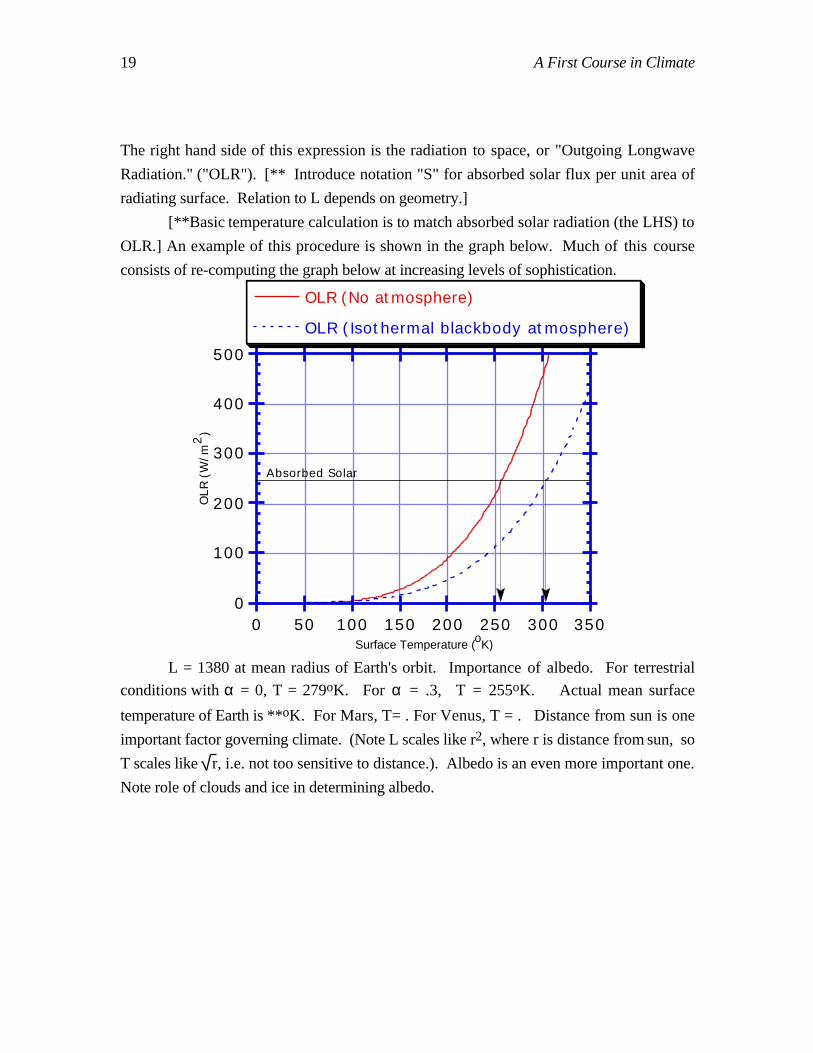
The right hand side of this expression is the radiation to space, or "Outgoing Longwave
Radiation." ("OLR"). [** Introduce notation "S" for absorbed solar flux per unit area of
radiating surface. Relation to L depends on geometry.]
[**Basic temperature calculation is to match absorbed solar radiation (the LHS) to
OLR.] An example of this procedure is shown in the graph below. Much of this course
consists of re-computing the graph below at increasing levels of sophistication.
0
100
200
300
400
500
0
OLR
(W
/m2
)
50 100 150 200 250 300
OLR (No atmosphere)
OLR (Isothermal blackbody atmosphere)
Surface Temperature (oK)
Absorbed Solar
350
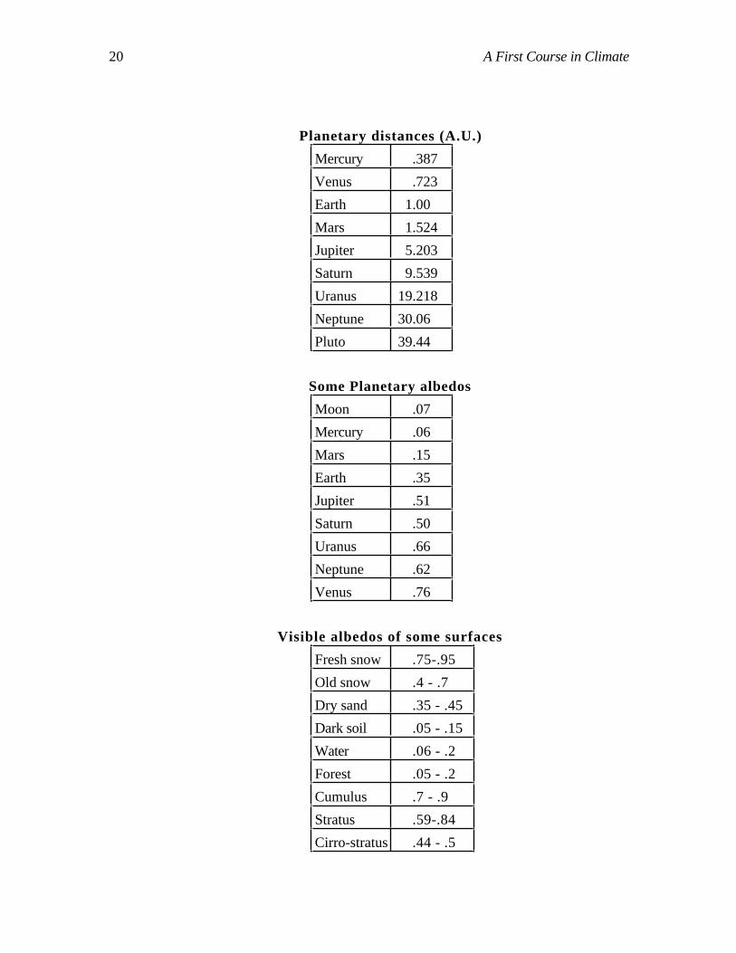
L = 1380 at mean radius of Earth's orbit. Importance of albedo. For terrestrial
conditions with α = 0, T = 279oK. For α = .3, T = 255oK. Actual mean surface
temperature of Earth is **oK. For Mars, T= . For Venus, T = . Distance from sun is one
important factor governing climate. (Note L scales like r2, where r is distance from sun, so
T scales like r, i.e. not too sensitive to distance.). Albedo is an even more important one.
Note role of clouds and ice in determining albedo.
20 A First Course in Climate
Planetary distances (A.U.)
Mercury .387
Venus .723
Earth 1.00
Mars 1.524
Jupiter 5.203
Saturn 9.539
Uranus 19.218
Neptune 30.06
Pluto 39.44
Some Planetary albedos
Moon .07
Mercury .06
Mars .15
Earth .35
Jupiter .51
Saturn .50
Uranus .66
Neptune .62
Venus .76
Visible albedos of some surfaces
Fresh snow .75-.95
Old snow .4 - .7
Dry sand .35 - .45
Dark soil .05 - .15
Water .06 - .2
Forest .05 - .2
Cumulus .7 - .9
Stratus .59-.84
Cirro-stratus .44 - .5
21 A First Course in Climate
[**Remarks on geometry and heat transport. The above is a "copper earth"
example. We did a global radiation budget, with uniform surface temperature. Rather
unrealistic to assume temperature uniform without atmosphere/ocean, since atmos/ocean
would be needed to move heat around and keep the temperature uniform. Rotation, and
"thermal inertia" help even out day/night cycle. Contrasting example of noontime
equatorial temperature. Equatorial temperature for no-atmosphere case, with rapid enough
rotation to average out the temperature. around the Equatorial belt. So, even without
radiative effects, atmosphere/ocean is having a profound effect on the global temperature,
by evening out such contrasts in time and space. Remark: T4 is a nonlinear function.
Effects of temperature variations on OLR. Give latitudinal temperature range of earth, and
say what effects on OLR would be based on T4. Point out that OLR(T) for real earth may
be rather different (come back to this later). Temperature variations act to increase OLR
(for a fixed global mean temperature), and hence give a cooler planet. Conversely, a planet
with a more uniform temperature will tend to have a warmer mean temperature than one
with large seasonal and/or latitudinal gradients. Note implications for positive mixing
feedback in warm climates like the Cretaceous. Will return to this subject in Chapter **.]
Now let's clothe our bare planet with an atmosphere. At this point, we need to
consider the spectrum of solar and terrestrial radiation. There is little atmospheric
absorption of solar radiation (on Earth 19% is absorbed in atmosphere, 51% at the ground,
the rest is scattered back to space). There is little scattering of outgoing IR. The basic
picture is that the Earth absorbs solar radiation (mostly at the surface of the planet) and re-
radiates energy as IR, some of which is absorbed by the atmosphere and re-radiated (as IR)
upward to space and downward back to the surface.
Often, in this course, it will be sufficient to idealize the atmosphere as being
transparent to solar radiation. A notable exception will be the need to consider absorption of
ultraviolet radiation as an explanation of the thermal structure of the Earth's stratosphere.
We will be able to get by primarily with IR radiative transfer theory. Solar scattering by the
atmosphere will not be treated in detail; we incorporate it only through a reflection
coefficient, to be thought of as primarily due to clouds.
Consider an "atmosphere" which is a black body transparent to the solar radiation
but which absorbs (and re-emits like a black body) all terrestrial IR. A key point is that the
atmosphere has two sides, a bottom and a top, and therefore radiates from both sides. For
simplicity, assume both IR albedo is zero. Then
22 A First Course in Climate
1-α4 L + σTa4 = σ Te4
σ Te4 = 2 σ Ta4 , i.e. Ta4 = Te4 / 2
Hence, the planetary surface is warmer than the no-atmosphere case by a factor of 21/4.
(i.e. with zero albedo, get Te = 332oK (Hot! Even with 30% albedo, get Te = 303.5).
Actual mean surface temperature of the Earth is about 285K, currently. Note Ta = 279oK,
the "old" temperature of the earth. Combine the two equations. OLR is σTa4. Or, could
use second equation, and get OLR as function of Te. This is another instance of "OLR
thinking," and is depicted in the [**blackbody graph] above.
Consistency problem: Atmosphere is colder than the planetary surface. Hot air will
form at the bottom and rise, giving vertical mixing. Simple "radiative-convective" (box)
model.1-α4 L + σTa4 = σ Te4 - k(Ta - Te)
σ Te4 = σ Ta4 + k(Ta - Te)
[**Solve for Te and sub in 2.2.xa; surface flux drops out. Ta stays fixed, but surface
temperature varies. This shows that thermal coupling between the atmosphere and surface
is a key factor in governing surface temperature. If coupling is strong, then the
"greenhouse effect" is not very potent (at least for an isothermal atmosphere.)]
[**Ice-albedo feedback. Equilibrium equatorial and global average temperature of
ice-covered earth. Multiple equilibria. How to escape from ice-covered earth?]
3.3 Partial absorption: Emissivity and Kirchoff's Laws
[**Dealing with partial absorption of IR. Why a black body is called "black."
Emissivity. Kirchoff's law: absorption coefficient = emissivity. Thermodynamic
derivation. Derivation via time-reversibility.]
[**Applications of Kirchoff's law. Black-body atmospheric greenhouse effect for
emissivity < 1. Skin temperature and the stratosphere. Effect of solar heating on the skin
temperature — why a small solar heating has a big warming effect on the stratosphere.]
3.4 Making sense of the isothermal slab-atmosphere model
[**Basic question is whether we can make any sense of the slab atmosphere model,
when applied to a real atmosphere which is manifestly non-isothermal. Can't discard it,
because it seems to give reasonable temperatures for e=1.]
[**Difficulty of explaining Venus temperature with isothermal slab model,
especially in view of its high albedo. Venus surface temperature is 753oK, which is
23 A First Course in Climate
actually hotter than Mercury. What is missing? Compressibility effects of atmosphere
(implies T decreases with height even if atmosphere is "well mixed" in vertical), combined
with unequal radiation from "top" and "bottom" of atmosphere. Thick atmosphere of
Venus: 88 atmospheres of mostly CO2. Basic model for optically thick case. Radiating
level H. σT(H)4 balances S. Then extrapolate along adiabat (because there is a
troposphere, which is mixed) to get the surface temperature. Venus has so much absorber
that the radiating level is moved high up on the adiabat.]
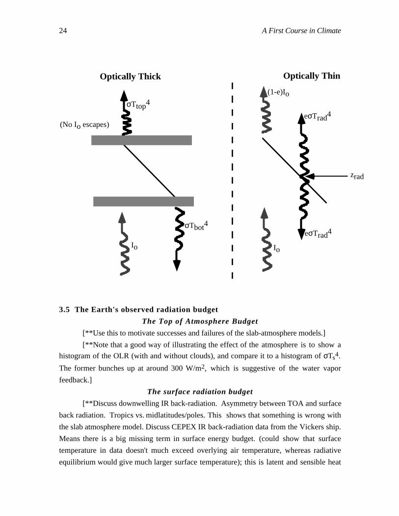
[**Some "handwaving" estimates of greenhouse warming for optically thick vs.
optically thin cases, assuming temperature goes down linearly with height. For optically
thin case, assume radiation out top and bottom of atmosphere is the same, and is given by
an effective radiating temperature comparable to a mid tropospheric value. This also yields
an estimate of the tropopause height: basically the atmosphere adjusts the mean
atmospheric temperature by adjusting the tropopause height. Does this also eliminate the
drive to instability at the ground? Will see later.
For optically thick case, put a black body at the top and at the bottom, and radiation
is asymmetrical. Behavior is not approximated by an isothermal model. Will see in Section
4 that temperature decrease with height is critical to the way the Greenhouse effect operates.
Earth is in the middle ground between Mars and Venus with regard to how the greenhouse
effect operates.]
24 A First Course in Climate
zrad
σTtop4
σTbot4
eσTrad4
Io Io
eσTrad4
(1-e)Io
(No Io escapes)
Optically Thick Optically Thin
3.5 The Earth's observed radiation budget
The Top of Atmosphere Budget
[**Use this to motivate successes and failures of the slab-atmosphere models.]
[**Note that a good way of illustrating the effect of the atmosphere is to show a
histogram of the OLR (with and without clouds), and compare it to a histogram of σTs4.
The former bunches up at around 300 W/m2, which is suggestive of the water vapor
feedback.]
The surface radiation budget
[**Discuss downwelling IR back-radiation. Asymmetry between TOA and surface
back radiation. Tropics vs. midlatitudes/poles. This shows that something is wrong with
the slab atmosphere model. Discuss CEPEX IR back-radiation data from the Vickers ship.
Means there is a big missing term in surface energy budget. (could show that surface
temperature in data doesn't much exceed overlying air temperature, whereas radiative
equilibrium would give much larger surface temperature); this is latent and sensible heat
25 A First Course in Climate
flux, which we will discuss later. How to close the imbalance? Defer full discussion of
surface energy balance for later. ]
[**This is a good place to point out that the observed surface temperature is usually
close to the overlying air temperature, so thermal coupling is tighter than radiation would
imply. Main exceptions are over dry deserts. Suggests evaporation is the culprit
("steaming gun.") Will return to this in Section **.]
3.6 Ice Albedo Feedback
[**Three great feedbacks: CO2 thermostat, water vapor, and ice albedo. In this
section we will consider a simple model of the ice-albedo feedback. Simply put, the idea is
that if you make a planet a bit colder, more of it is covered by ice. Then, since ice has a
higher albedo than water or land, less solar energy is absorbed and the planet cools further.
This can lead to many interesting phenomena. For simplicity, we will illustrate the
working of the ice-albedo feedback in a planet with an atmosphere that has no greenhouse
effect.]
Suppose that the planet is ice covered from latitude φi to the poles, in each
hemisphere. Then the fractional area covered by ice is 1- sinφi. If αo is the albedo of the
ice-free surface and αi is the albedo of the ice covered surface, the planetary albedo is
α = αo sin φi + αi (1 - sinφi)
Next define a mean surface temperature by σ T—4 = (1-α)L/4. The meridional temperature
gradient profoundly affects the ice-albedo feedback, so rather than assuming the planet to
be isothermal, we allow for a specified meridional temperature profile
T = T—
+ ∆T ( 12 – sinφ)
where φ is the latitude and ∆T is a specified constant. This profile has an area-weighted
mean of T—
. The ice margin is determined by the latitude where T = Tf, where Tf is the
freezing temperature (273.15 for fresh water). From this we infer that the ice margin is at
sinφi = 12 +
T—
- T f
∆T
From this we compute the coalbedo as a function of mean surface temperature
(1-α) = ( 1 - 12 (αo+αi)) + (αi-αo)
T—
- T f
∆T
[**Cut this off at (1-αi) at cold temperatures, and (1-αo) at warm temperatures so as to
keep sinφi in its allowable range.]
26 A First Course in Climate
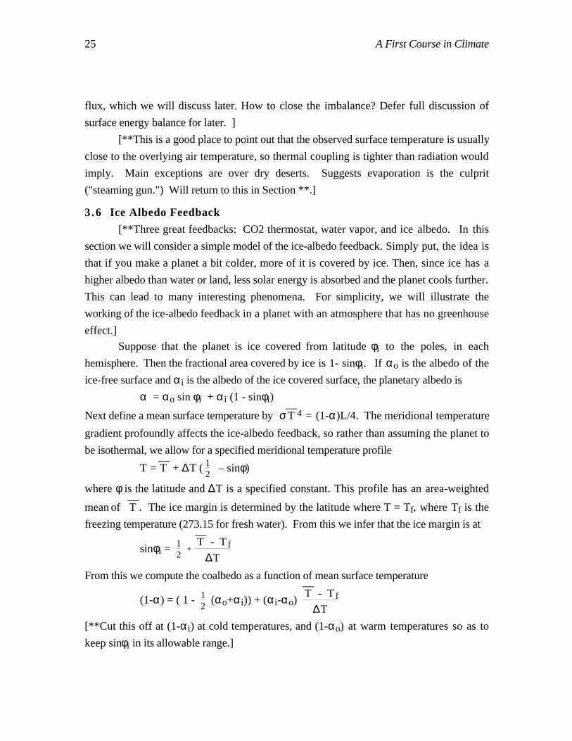
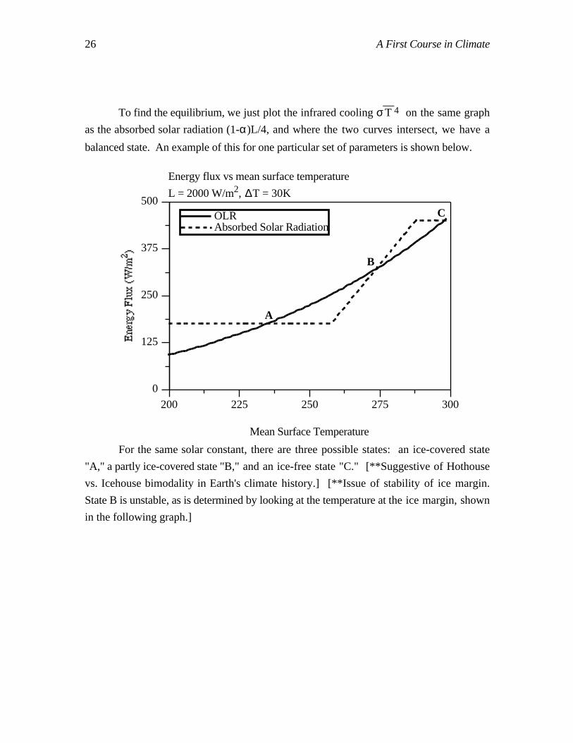
To find the equilibrium, we just plot the infrared cooling σ T—4 on the same graph
as the absorbed solar radiation (1-α)L/4, and where the two curves intersect, we have a
balanced state. An example of this for one particular set of parameters is shown below.
200 225 250 275 300
0
125
250
375
500
Mean Surface Temperature
Energy flux vs mean surface temperature
L = 2000 W/m2, ∆T = 30K
A
B
C OLR Absorbed Solar Radiation
For the same solar constant, there are three possible states: an ice-covered state
"A," a partly ice-covered state "B," and an ice-free state "C." [**Suggestive of Hothouse
vs. Icehouse bimodality in Earth's climate history.] [**Issue of stability of ice margin.
State B is unstable, as is determined by looking at the temperature at the ice margin, shown
in the following graph.]
27 A First Course in Climate
0.00 0.25 0.50 0.75 1.00
250
260
270
280
290
sine(ice margin latitude)
B
Ice margin temperature
L = 2000 W/m2, ∆T = 30K
A
C
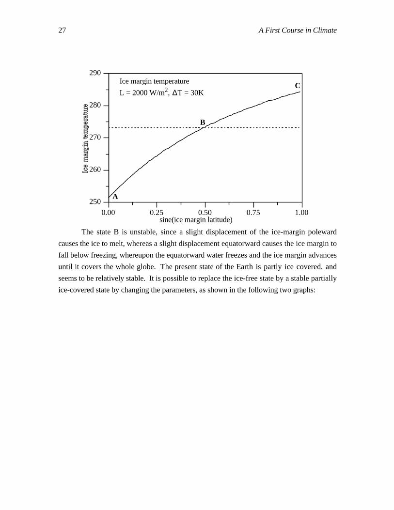
The state B is unstable, since a slight displacement of the ice-margin poleward
causes the ice to melt, whereas a slight displacement equatorward causes the ice margin to
fall below freezing, whereupon the equatorward water freezes and the ice margin advances
until it covers the whole globe. The present state of the Earth is partly ice covered, and
seems to be relatively stable. It is possible to replace the ice-free state by a stable partially
ice-covered state by changing the parameters, as shown in the following two graphs:
28 A First Course in Climate
200 225 250 275 300 325
0
125
250
375
500
625
Mean Surface Temperature
Energy flux vs mean surface temperature
L = 2050 W/m2, ∆T = 60K
AB
C
OLR Absorbed Solar Radiation
0.00 0.25 0.50 0.75 1.00
267.5
270.0
272.5
275.0
277.5
sine(ice margin latitude)
L = 2050 W/m2, ∆T = 60K
A
B
C
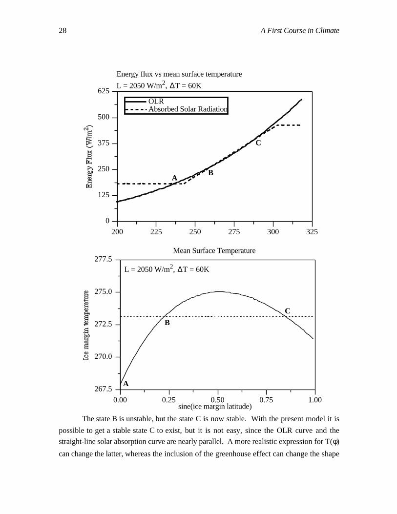
The state B is unstable, but the state C is now stable. With the present model it is
possible to get a stable state C to exist, but it is not easy, since the OLR curve and the
straight-line solar absorption curve are nearly parallel. A more realistic expression for T(φ)
can change the latter, whereas the inclusion of the greenhouse effect can change the shape
29 A First Course in Climate
of the OLR curve. Both effects can help make the stable state with glaciated polar regions
more robust.
[**Do a third case, with small dT. In this case, the partially ice covered state can be
the stable one.]
[**Fragility of the polar ice state suggests just a bit of change could cause it to be
lost, leading to an ice-free state. Suggestive of Cretaceous and other hothouse climates.]
[**Discuss climate senstitivity for state C. Change L, and look how T changes,
with and without ice feedback. Relevance to global warming.]
30 A First Course in Climate
4. One-dimensional radiative-convective models4.1 IR radiative transfer in a continuously stratified grey-gas atmosphere
[**Definition of optical depth, and what it means.] Usually, we choose zo such
that τ=0 at the ground. Since the emissivity/absorptivity is more or less proportional to the
mass of absorbing matter encountered by the light beam, it is most natural to express the
specific emissivity in terms of the density of the medium, so
τ(z) = ∫z0
z
ρ(z) κ(z) dz = ∫p
po
κ(p) dp/g
where κ is now the emissivity expressed in units of 1/( mass/area) ,i.e. it is a kind of mass
cross-section. The second equality holds by virture of the hydrostatic relation. Note that if
κ is bounded, then the atmosphere has a finite optical depth, since it has a finite mass.
[**Note: The following expressions are for parallel beam radiation. In reality, IR radiation
is diffuse, i.e., it comes in equal intensities at all angles. This can be handled by just re-
defining optical depth with an apropriate proportionality constant out front.]
Schwartzschild equations for IR radiation, in terms of optical depth (grey
atmosphere):dI+
dτ = - I+ + σT4
dI-
dτ = I- - σT4
The general solution for arbitrary T(z) (re-expressed as a function of τ) is
I+ = ∫τo
τ σ T(τ')4 e -(τ-τ ') dτ' + Ae-τ
and mutatis mutandum for I-. A is a constant of integration used to satisfy one boundary
condition on I+, which is usually that I+ at the ground is equal to the blackbody radiation
flux emitted by the planetary surface. There is a similar constant of integration and
boundary condition (usually applied at the "top" of the atmosphere, stating that there is no
incoming IR, i.e. I- = 0 at the "top") for I-.
The formula for the intensities states that the radiation is a weighted average of the
blackbody radiation, taken over a couple optical depths. If the atmosphere is "optically
thick", i.e has a large difference in τ between the top and bottom, then the atmosphere
radiates to space at the temperature of the "top" of the atmosphere, and to the ground at the
31 A First Course in Climate
temperature of the (usually colder) "bottom" of the atmosphere. If the atmosphere is
"optically thin", then there isn't so much asymmetry between the outgoing flux and the flux
radiated to the planetary surface, and both are connected to the "mean temperature" of the
atmosphere as a whole. [**Implies difference between Venus and Earth. Optical thickness
of Venus atmosphere is why it can support such a strong greenhouse effect.]
[**Radiation flux convergence and heating rates.] For a given profile of I+(τ) and I-
(τ), the system will not ordinarily be in radiative equilibrium; that is, the net amount of
radiation going into the slab between τ and τ+dτ is not equal to the amount leaving. Thus
the slab will heat up or cool down. The net heating rate (in units of energy absorbed per
unit optical depth) is
H = – d
dτ (I+ - I-)
How to turn this heating into more physical units (degrees/day). ]
Now, let's do a few calculations to exercise our facility with the Schwartzschild
equations, and get a feel for their consequences.
[**Show that an isothermal slab radiates like a black body when it gets optically
thick. Compute cooling profile for such a slab. Note relevance to cloud top cooling in
stratus decks. An alternate form of this calculation is an isothermal slab in contact with a
surface of the same temperature.]
[**Discuss net radiation in and out for isothermal body and for body with T(z).
Asymmetric downward and upward radiation for T(z). Discuss optically thick limit for
T(z) = T0 - γz. This is a more precise derivation of the picture we sketched out in the
previous chapter.] [**Surface greenhouse effect for general optically thick atmosphere with
T(z) decreasing with height. Decrease of T with height due to vertical mixing and to
compressibility. This might be a good lead-in to discussion of why surface heating creates
a troposphere. Surface must get rid of S, as well as the incident IR back radiation.]
Suppose T(z) is decreasing with height, at least near the ground, and that the atmospheric
temperature at the ground, T(0) is equal to the ground temperature Ts. [**T decreasing
because of tropospheric mixing, favoring an adiabatic lapse rate. T(0) equalizes to Ts
because of thermal coupling to ground.] The downward IR flux at the ground is
I-(0) = σ ∫0
∞ T4 e -τ dτ
and the surface energy balance is
F + I-(0) = σTs4 = σT(0)4
32 A First Course in Climate
where F is the net solar flux reaching the ground (allowing for all albedo, absorption and
geometric effects). Now, if the atmosphere is optically thick, then I-(0) is sensitive only to
the temperature profile near the ground; thus we can write T = T(0) - γz, where γ is the
lapse rate. Further, T4 can be linearized about T(0), since z is small over the range where
the optical depth is order unity (this is in fact what we mean by optically thick). Thus,
I-(0) = σT(0)4 - 4σT(0)3 γ z*
where
z* = ∫0
∞ z e -τ dτ
The depth z* is our measure of how optically thick the atmosphere is, and goes to
zero as the atmosphere becomes thicker. Thus, optically thick atmospheres radiate to the
ground at a temperature that is only slightly less than the surface temperature. [**If there
were no convective heat transport, surface would warm to be much warmer than overlying
atmosphere; strong convection would set in to rectify this. Write down surface energy
budget. Convective heat fluxes would bring Ts to be similar to T(0). In that case, very little
of the incoming solar energy is lost by reradiation to the atmosphere. The net IR cooling of
the surface is weak (quote some typical values, for observations and for a dry atmosphere
with present CO2), and the dominant balance is between solar heating and convective heat
flux (on Earth, mostly latent, at least in Tropics).]
[**Computation of OLR for an adiabatic greygas atmosphere. This is the first of
three basic climate calculations: (1) "all troposphere" planet, (2) "all stratosphere" planet,
(3) patching a troposphere into a stratosphere. Should this be here or further down? We
haven't really discussed yet the way radiation drives the thermal instability that creates the
troposphere.] Assuming the atmosphere to be optically thick, so that no radiation from the
ground directly escapes to space, the OLR for an adiabatic atmosphere with (constant)
potential temperature θ is
I+(τ∞) = ⌡⌠
0
τ∞
σ{θ (ppo
)R/Cp }4 e - (τ∞ - τ) dτ
We must eliminate p from this, to get a closed form expression. To do this, use dτ = - κdp/g, with constant κ The expression for OLR becomes
33 A First Course in Climate
I+(τ∞) = σθ4 (τ∞)-4R/Cp ∫0
∞ ζ4R/Cp e- ζ dζ
where we have introduced the dummy variable ζ = τ∞ - τ. We have also replaced the upper
limit of integration with ∞ because we are assuming that τ∞is large, so that given the
exponential weighting in the integrand, it makes little difference if it is infinite or merely
very large. The integral in the OLR expression is now only a function of R/Cp. [**Give
value for 2/7 (air); 1.06. Will be close to unity. Note that for fixed temperature, OLR
decreases to zero as atmosphere is made more optically thick. Note also that θ is the
surface air temperature, by definition of po . Hence, balancing OLR against absorbed solar
radiation, the low level air temperature increases without bound as the atmosphere is made
more optically thick. Contrast with result for isothermal slab model of the greenhouse
effect. Note that lapse rate is g/Cp, so by changing Cp with R fixed, one can examine the
effect of lapse rate. For small lapse rate R/Cp becomes small, and the greenhouse effect
vanishes (if the surface temperature equals the low level air temperature.)
Note that the upper part of the all-troposphere planet is hard to create or maintain.
If there is any heating of it at all, then because of its low pressure it will acquire a very large
θ. This will prevent low level air parcels from being able to penetrate, and a stratosphere
will form to cap the atmosphere. ]
[**Use formula to try to estimate surface temperature on Venus. Show what
optical thickness would be needed to get surface temperature. What is the optical thickness
for a 80 bar pure CO2 atmosphere? To answer this question, need to look in more detail at
the way gases actually absorb IR radiation.]
[**Effect of clouds on OLR and surface temperature. Implications for remote
sensing. Compute surface temperature for an adiabatic atmosphere, if we put clouds at the
tropopause. Importance of cancellation between albedo effect of clouds and greenhouse
effect of clouds.]
4.2 Some bad news and some good news: Non-grey effects
[**Reader should now be wondering: OK, just how optically thick is the Earth's
atmosphere really? How does the emissivity depend on the amount of CO2? Answer is
more complicated than one would like it to be.]
[**Water vapor and CO2. Importance of window channels and saturation of
absorption bands. Importance of the water vapor continuum.]
34 A First Course in Climate
[**Non-grey gases. No longer have exponential decay of radiation. Discuss
structure of band absorption. Discuss I(z) for average over a Lorentz shape. Discuss
pressure dependence of band width (pressure broadening). For separated bands, net
absorption (for constant mass and composition) is proportional to pressure. Discuss
continua. Provide quantitative data on net absorption.]
[**Discuss Vickers FTIR data.]
These complications are bad news, because they mean that a very complicated
radiation model is needed to compute the IR radiation profile [**Need to do calculation for
separate τ for each ν, then sum up. In practice, do calc. for each band or group of bands].
This may be bad news for climate modelers, but it is good news for the life of the Earth,
and for other would-be life supporting planets elsewhere in the Universe. [**Exponential
absorption characteristic of a grey gas would make climate very sensitive to concentration
of absorbers. Earth would get very warm easily. Estimate what doubling CO2 would do
to temperature if CO2 were a grey gas. The saturation of the greenhouse effect is what
makes CO2 a good thermostat.]
[**Using the NCAR radiation model, take a given (observed) T(p) and show OLR
and surface back-radiation as a function of CO2 (for a dry atmosphere), and as a function
of relative humidity (with dry stratosphere) for a no-CO2 atmosphere.]
[**Note, pressure corrected CO2 in present earth atmosphere is about 1 m (check
this). Thus, doubling or tripling CO2 is in a range where emissivity is not changing much.
Without water vapor and cloud feedback, the CO2 warming would be pretty negligable.
Difficulty of explaining warm Venus with CO2 alone.]
[**To do CO2 absorption on Venus, the effects of myriad very weak absorption
bands must be summed up. Not clear that we can account for sfc. temperature by CO2
absorption alone. Is there water vapor on Venus? Could clouds be the answer? Note
liquid droplets should act like black bodies. Putting clouds at a low pressure part of the
atmosphere would give a warm surface temperature, by moving the emitting surface high
up. How "blackbody" are the Venus clouds? What pressure level are they located at?]
4.3 Radiative equilibrium
Let's consider an atmosphere which is in local radiative equilibrium with the IR
radiated from the planetary surface. We assume it is perfectly transparent to the incident
solar radiation, so that the only heating of the atmosphere is due to IR absorption. [**First
consider greygas case, which we can do analytically.] Local radiative equilibrium implies
H =0, so (I+ - I-) is a constant independant of τ. If τ∞ is the optical depth of the top of the
35 A First Course in Climate
atmosphere (z = ∞), then I-(τ∞) = 0. Further, since the planet as a whole must be in
radiative equilibrium with the incoming solar flux F, then I+(τ∞) = S. Thus, (I+ - I-) = S
everywhere. Further, upon adding the differential equation for I+ and I-, we obtaind
dτ (I+ + I-) = -(I+ - I-) = -S,
so (choosing a constant of integration to satisfy the upper boundary condition)
(I+ + I-) = -S(τ - τ∞ - 1)
Finally, subtracting the equations for I+ and I- and using H = 0, we obtain the temperature
as a function of τ:
2σT4 = (I+ + I-) = S(1 - τ +τ∞)
In radiative equilibrium, then, the atmospheric temperature decreases with optical depth.
The rapidity with which the temperature decreases with height depends on the distribution
of absorbers, which determines the function τ(z). [**Give some examples of τ(z)
suggesting that T is roughly isothermal in the stratosphere. Discuss limiting temperature at
the top of the atmosphere. Note that it is colder than the temperature of a no-atmosphere
blackbody in equilibrium with S, by a factor 2-1/4. This is independent of whether the
atmosphere is optically thick or optically thin. It is a characteristic temperature of a planet.
Discuss values for Earth, Mars, Venus and Jupiter, and compare with observed upper-
atmosphere values. On Earth, the comparison reveals the effect of ozone heating. ]
With the above formulae, we have I-(0) and therefore can complete the surface
energy budget to obtain the ground temperature Ts. Since I+(0) = σTs4, the surface energy
budget becomes:
S + I-(0) = σTs4 , i.e. , S + S(1+τ∞) - σTs4 = σTs4
and the surface temperature is given by
Ts4 = S
σ(1 + τ∞/2)
When the atmosphere is optically thin (τ∞ = 0), then the surface temperature reduces to the
no-atmosphere radiative equilibrium. The ground temperature increases without bound as
the optical thickness of the atmosphere increases. For τ∞ = 2, we obtain the same
greenhouse warming (i.e. surface temperature increases by a factor of 21/4) as for the
isothermal slab atmosphere; however, the surface temperature continues to increase as we
make the atmosphere thicker, because the radiative equilibrium atmosphere is not
isothermal. Its top is colder than its bottom, and so it radiates to the ground at a higher
temperature than it radiates to space.
36 A First Course in Climate
Note that
T(0)4 = 1+τ∞ 2+τ∞
Ts4
Hence, as in the case of the isothermal slab atmosphere, there is a convective instability due
to the surface being warmer than the atmosphere in contact with it. The strong convection
inevitably ensuing will transport heat from the surface to the atmosphere, warming the
atmosphere and cooling the surface until the lower atmosphere temperature becomes similar
to the overlying air temperature. Such convection will also tend to mix up the atmosphere,
though, leading to a roughly adiabatic troposphere. [**For consistency, need to patch
together a troposphere with a stratosphere, which we will do shortly.]
[**Do optically thick and optically thin limit. Optically thin limit reduces to the
isothermal slab model. For optically thick limit, surface temperature increases without
bound.]
Heating at the ground is not the only possible source of instability though.
Instability occurs if the temperature falls rapidly enough with height that the potential
temperature decreases with height. Letting ζ = -ln(p/ps), then for an adiabatic atmosphere
d(lnT)/dζ = -R/Cp, and any atmosphere with a more negative gradient will be unstable.
Since dln(T)/dz = (dln(T)/dτ)(dτ/dζ), there can be convective instabilities interior to the
atmosphere if dτ/dζ is large enough. Consider first the case of a uniform-composition
atmosphere, ignoring the effects of collisional broadening [**NB have we defined
collisional broadening yet?] For this case, we approximate τ = κ (ps - p)/g, where ps is
the surface pressure and κ is some constant. Then, dτ/dz = κ ρ, using the hydrostatic
relation. Further, we can evaluate dT/dτ using the formula for the radiative equilibrium
temperature profile. Namely,
8σT3 dT
dτ = –S
sod
dτ ln(T) = –
1
4(1+τ∞ -τ)
Note that S has dropped out of this expression, so that the stability is independent of the
insolation. Next multiply both sides by dτ/dζ, and make use of the fact that dτ/dζ = κp/g.
Thus,
d
dζ ln(T) = –
κp/g
4(1+τ∞ -τ)
37 A First Course in Climate
So far, this expression is valid even if κ is a function of p. In the special case that κ is
constant, then κp/g = τ∞ - τ, and the right hand side is a function of τ alond. This function
of τ has a maximum at the ground, which approaches 1 in the limit of an optically thick
atmosphere. It goes to zero at the top of the atmosphere, so that the radiative equilibrium is
always stable sufficiently high up. Now lets take the "worst case" and ask whether the
lapse rate is unstable (more negative than –R/Cp) near the ground in the limit of very large
τ∞. The magnitude of the lapse rate near the ground in this case is 1/4. Hence, the
atmosphere is internally unstable if 1/4 > R/Cp. Air, with R/Cp = 2/7, just misses being
unstable. Hence, we must look to other means to generate the stirring to create the Earth's
troposphere. [**Comment on other substances; pure water vapor, CO2, hydrogen,
helium.]
[**Discuss when a stable stratosphere is possible. Discuss effects of collisional
broadening (via problem?). How do non-grey effects change this? On Jupiter and Saturn,
where there is no surface, destabilization creating a troposphere must arise from internal
destabilization, or from an internal heat source. Could conceivably be due to solar
absorption, but since the available light decreases with depth (as in an ocean), this would
tend to stabilize things (cf. problem on effect of absorption.)]
[** (moisture effects important in determining size of this factor, since moisture
decreases strongly with height). Discuss role of moisture and clouds in making dτ/dz large
and destabilizing the atmosphere. Discuss dτ/dz for a saturated radiative equilibrium
atmosphere. Is it unstable?]
[**Approximation of convection by "convective adjustment." Troposphere (well
mixed vertically, due to convection) and Stratosphere (not well mixed, roughly in local
radiative equilibrium). ]
[** Is there always a drive to convection from below? Have seen this twice now.
For optically thick atmosphere, IR cooling of ground is weak, and ground will always heat
up and stir convection. What happens in the optically thin limit?]
[**Nongrey effects. Give some radiative-equilibrium solutions using NCAR
model, and compare with grey gas. Discuss optically thin vs. optically thick limit.]
4.4 Coupling radiation to convection: Making the Troposphere
[**Dry radiative convective model. Full problem: (a) T(0) = Ts (finesses need to
solve surface energy budget), (b) T continuous at tropopause, (c) Strat in radiative
equilibrium, (d) Surface in radiative equilibrium, (e) Troposphere as a whole is in radiative
38 A First Course in Climate
equilibrium, though not locally at each height. Form of solution very dependent on the
vertical distribution of the absorbers (for an example, do a pure CO2 atmosphere).]
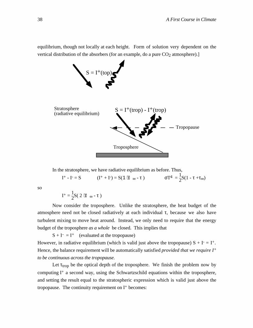
Tropopause
Stratosphere(radiative equilibrium)
Troposphere
S = I+(top)
S = I+(trop) - I+(trop)
In the stratosphere, we have radiative equilibrium as before. Thus,
I+ - I- = S (I+ + I-) = S(1 + τ∞ - τ ) σT4 = 12S(1 - τ +τ∞)
so
I+ = 12S( 2 + τ∞ - τ )
Now consider the troposphere. Unlike the stratosphere, the heat budget of the
atmosphere need not be closed radiatively at each individual τ, because we also have
turbulent mixing to move heat around. Instead, we only need to require that the energy
budget of the troposphere as a whole be closed. This implies that
S + I- = I+ (evaluated at the tropopause)
However, in radiative equilibrium (which is valid just above the tropopause) S + I- = I+.
Hence, the balance requirement will be automatically satisfied provided that we require I+
to be continuous across the tropopause.
Let τtrop be the optical depth of the troposphere. We finish the problem now by
computing I+ a second way, using the Schwartzschild equations within the troposphere,
and setting the result equal to the stratospheric expression which is valid just above the
tropopause. The continuity requirement on I+ becomes:
39 A First Course in Climate
12S ( 2 + τ∞ - τtrop ) = ∫
0
τtrop
σT4 exp(-(τtrop-τ))dτ + σTs4 exp(-τtrop)
We will assume that there is strong enough surface turbulent flux that Ts = T(0).
Further, since the troposphere is on the (dry) adiabat, we have (in the troposphere)
T = Ttrop (p
ptrop)R/Cp
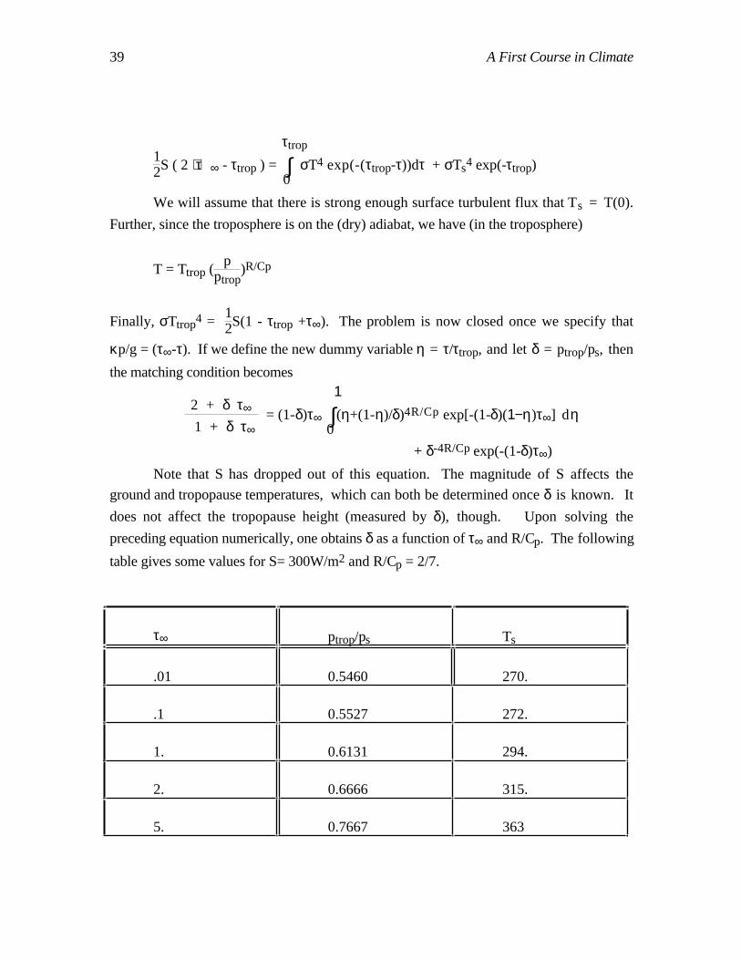
Finally, σTtrop4 = 12S(1 - τtrop +τ∞). The problem is now closed once we specify that
κp/g = (τ∞-τ). If we define the new dummy variable η = τ/τtrop, and let δ = ptrop/ps, then
the matching condition becomes
2 + δ τ∞
1 + δ τ∞ = (1-δ)τ∞ ∫
0
1(η+(1-η)/δ)4R/Cp exp[-(1-δ)(1−η)τ∞] dη
+ δ-4R/Cp exp(-(1-δ)τ∞)
Note that S has dropped out of this equation. The magnitude of S affects the
ground and tropopause temperatures, which can both be determined once δ is known. It
does not affect the tropopause height (measured by δ), though. Upon solving the
preceding equation numerically, one obtains δ as a function of τ∞ and R/Cp. The following
table gives some values for S= 300W/m2 and R/Cp = 2/7.
τ∞ ptrop/ps Ts
.01 0.5460 270.
.1 0.5527 272.
1. 0.6131 294.
2. 0.6666 315.
5. 0.7667 363
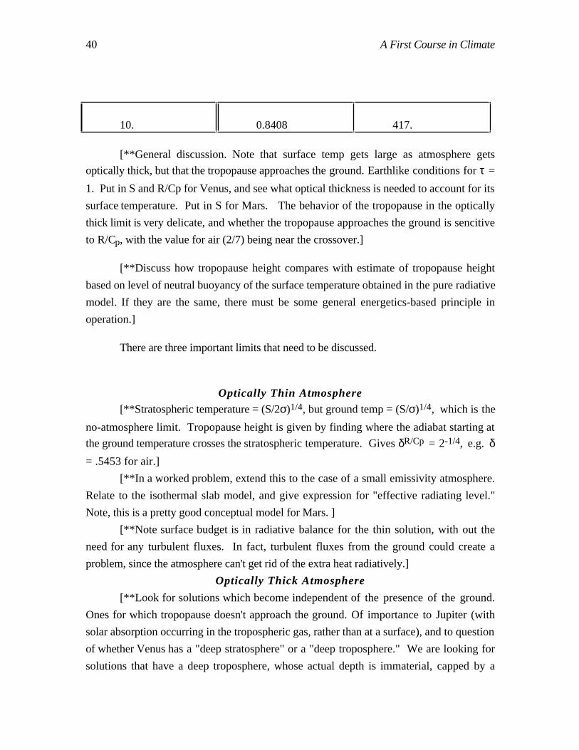
40 A First Course in Climate
10. 0.8408 417.
[**General discussion. Note that surface temp gets large as atmosphere gets
optically thick, but that the tropopause approaches the ground. Earthlike conditions for τ =
1. Put in S and R/Cp for Venus, and see what optical thickness is needed to account for its
surface temperature. Put in S for Mars. The behavior of the tropopause in the optically
thick limit is very delicate, and whether the tropopause approaches the ground is sencitive
to R/Cp, with the value for air (2/7) being near the crossover.]
[**Discuss how tropopause height compares with estimate of tropopause height
based on level of neutral buoyancy of the surface temperature obtained in the pure radiative
model. If they are the same, there must be some general energetics-based principle in
operation.]
There are three important limits that need to be discussed.
Optically Thin Atmosphere[**Stratospheric temperature = (S/2σ)1/4, but ground temp = (S/σ)1/4, which is the
no-atmosphere limit. Tropopause height is given by finding where the adiabat starting at
the ground temperature crosses the stratospheric temperature. Gives δR/Cp = 2-1/4, e.g. δ= .5453 for air.]
[**In a worked problem, extend this to the case of a small emissivity atmosphere.
Relate to the isothermal slab model, and give expression for "effective radiating level."
Note, this is a pretty good conceptual model for Mars. ]
[**Note surface budget is in radiative balance for the thin solution, with out the
need for any turbulent fluxes. In fact, turbulent fluxes from the ground could create a
problem, since the atmosphere can't get rid of the extra heat radiatively.]
Optically Thick Atmosphere
[**Look for solutions which become independent of the presence of the ground.
Ones for which tropopause doesn't approach the ground. Of importance to Jupiter (with
solar absorption occurring in the tropospheric gas, rather than at a surface), and to question
of whether Venus has a "deep stratosphere" or a "deep troposphere." We are looking for
solutions that have a deep troposphere, whose actual depth is immaterial, capped by a
41 A First Course in Climate
stratosphere of finite optical thickness. Basically, we are putting a stratospheric hat atop
the all-troposphere planet we discussed in Section **.]
For these solutions (if they exist), the transmission term in the tropospheric energy
balance is negligible. Since the I+ coming up from the troposphere is sensitive only to the
first few units of optical thickness in the troposphere, the optical depth of the atmosphere as
a whole becomes irrelevant, and so we choose ∆τ = τ∞ - τtrop as our basic parameter rather
than τ∞. Note that ∆τ is the optical thickness of the stratosphere. We introduce a new
dummy variable η = τtrop-τ, whence (p/ptrop) = 1 + η/∆τ. Because of the exponentially
decaying weighting, we are also free to integrate to infinite optical depth into the
troposphere. The resulting balance condition becomes
2 + ∆τ
1 + ∆τ = ∫
0
∞ ( 1 + η/∆τ)4R/Cp exp(-η ) d η
The left hand side approaches 2 for small ∆τ, and becomes 1 + 1/∆τ for large ∆τ. The right
hand side becomes
∆τ -4R/Cp ∫0
∞ η4R/Cp exp(-η ) d η
small ∆τ, which is proportional to Eq. (**) which we derived for the OLR of an all-
troposphere optically thick atmosphere. For our purposes, the important thing is that this
becomes infinite, so that the RHS curve of the energy balance starts out above the LHS. If
the RHS is below the LHS at large ∆τ, than a crossing point is assured.
At large ∆τ, the RHS integral becomes
∫0
∞ (1 + (4R/Cp) η/∆τ) exp(-η ) = 1 +
4R/Cp
∆τ
Hence, crossing is assured whenever 4R/Cp < 1. Remarkably, this is also the threshold
for a deep radiative equilibrium atmosphere to go gravitationally unstable on its own
without the necessity of surface heating. [**Nature is being kind and consistent. In just the
case where a deep stratosphere is unstable, a solution with an infinite-depth troposphere
becomes possible.] As for the instability criterion, dry air, with R/Cp = 2/7, just misses
allowing a deep troposphere solution. [**Give values for pure CO2 (relevant to Mars and
Venus), and point out importance of variation of Cp with temperature. Give values for
pure water vapor (steam atmosphere; runaway greenhouse). Give values for
hydrogen/helium mix. (Jupiter and Saturn). ]
42 A First Course in Climate
[**Insert graph of LHS and RHS for 3 values of R/Cp .]
[**What happens in the case where there's no deep-troposphere solution: What is
going on in the optically thick limit is that the tropopause radiates upward at very nearly the
tropopause temperature, because of the optical thickness of the troposphere. However, the
upward radiation in the stratosphere cannot be matched to this. As a result, the tropopause
is forced downward until the troposphere is optically thin enough for its depth to affect the
radiation. Another way of looking at it is that the zero order match for the optically thick
case requires a high temperature (hence low) tropopause.]
[**Cautionary note: The delicacy of the tropospheric balance in the optically thick
case means that the answer will be very dependent on other perturbations to the system,
like collisional broadening or nongrey effects or solar absorption in the stratosphere. This
makes the optically thick case very challenging. Note that for Venus, R/Cp gives a shallow
strat for the upper air temperatures, but because of temp dependence of Cp crosses over to
the deep strat value.]
[**Are there multiple equilibria? Specifically, when there's no deep-troposphere
solution with a stratosphere, is the all-troposphere planet a possible solution? (yes -- this is
always available). Which one is preferred?]
[**Are these results on the behavior of tropopause height in a thick atmosphere well
known? Look up sources. There is a chance that this is a novel result. Goody doesn't
seem to mention it. Check updated references, and Venus references.]
Small Lapse Rate
[**Change lapse rate by changing Cp with R fixed, since lapse rate is g/Cp. As
lapse rate is reduced, the stratosphere gradually vanishes, and the solution reduces to the
all-troposphere case. Note that in this limit, the greenhouse effect goes away. The upper
atmosphere does get cold, but because this part is always optically thin (by virtue of having
low density), it doesn't succeed in bringing down the OLR.]
[**The lapse rate dependence holds the key to tropopause height variations on
Earth. We saw in Chapter 2 that the tropopause is higher in the tropics than in the
midlatitudes. The increased absorbed solar cannot account for this. Water vapor makes the
tropics more optically thick than the midlatitudes, but this effect would lower rather than
raise the tropopause. However, condensation lowers the lapse rate. This is the main
influence in raising the tropical tropopause.]
43 A First Course in Climate
[**Defer discussion of Ts - T(0). For now, we'll just empirically say that it's
mostly small. Discuss radiative balance of surface though, to show that the implied
turbulent fluxes from the surface are indeed from the surface to the atmosphere.]
The static stability problem. It is "easy" to understand why there is a troposphere
that is approximately well-mixed (adiabatic). But the Earth's troposphere, while nearly
adiabatic is actually slightly statically stable. That small difference between slightly stable
and slightly unstable makes a world of difference in the circulations. It is the key
difference between terrestrial type (stably stratified) and stellar type (convective)
circulations. On Earth, the static stability might (and probably does) have something to do
with moisture. However, dry atmospheres (Mars), and dry GCM's still produce a
statically stable atmosphere. (Show some data.) Why?
4.5 1D models of atmospheres with a condensible component.
[**Some illustrative examples concerning latent heat: (a) Time scale for
unbalanced solar radiation to evaporate the ocean. Note that this is pretty much the rate of
water flux out of the tropical ocean; however, the ocean doesn't disappear, because the
water is quickly rained out back into the ocean (or snowed onto ice caps which flow and
melt). (b) Amount of water that can be evaporated by the energy of a cometary impact. (c)
Megaton equivalent of 1cm of precip over 1 km2. (d) Heat balance of an atmosphere
condensing out onto a polar night ice cap. Note that the darkside of a tide-locked planet is
an extreme case of polar night. Atmosphere will tend to disappear to the nightside, but as
the atmosphere moves there it carries heat (latent and sensible) with it. Constraints on the
rate of mass flux into the polar night (σT4 = A-1 dM/dt; however, if T gets too large or
atmospheric pressure gets to low, condensation ceases (but then T goes down, in the
absence of other heat transports)). ]
[**Consider pure condensible atmosphere (like CO2 for Mars). As if Earth had
pure steam atmosphere. Tour of Ingersoll's "low mass atmospheres." Mars dry-ice cap is
a good example. How to "terraform" Mars.]
Water vapor as a greenhouse gas. IR radiative effects of water vapor. Collisional
broadening of absorption lines. Slab emissivities for water vapor; importance of non-grey
effects: why emissivity is not exponential in slab thickness. Relative role of water vs. CO2
as an IR absorber. Radiative properties of liquid water (continuum absorption) and ice;
implications for cloud IR emissivity.
Radiative properties of liquid water and water vapor in the visible spectrum.
44 A First Course in Climate
Why does a liquid ocean exist? Runaway greenhouse possibility. Surface pressure
if oceans were evaporated. How long would it take for oceans to condense back? What
would temperature be in the intermediate times?
[**Kombayashi - Ingersoll limit. Maximum OLR for a radiative equilibrium
atmosphere.
2σT4 = (1 + τ∞-τ)OLR
2σTtrop4 = (1 + κptrop
g ) OLR
OLR = 2σTtrop4
( 1 + κptrop
g )
but if the tropopause is at saturation, ptrop = e∞ exp(-L/(RTtrop)). Substituting in the
above, this implies an upper bound on OLR (except for unrealistically large temperatures).
All-troposphere case. Suppose vertical structure given by T = Tsat(p) (this is the
"moist adiabat" for a pure condensible atmosphere).
OLR = σTs4 e-τ∞ + ∫σT4 e -τ dτ
but for a "saturated" pure condensible atmosphere,
T = LR
1
ln(τ) - ln(κe∞/g)
The second logarithm in the denominator is so enormous that the first can essentially be
neglected. In the optically thick limit we then have (approximately)
OLR = σ(LR)4 1
[ln(κe∞/g)]4 = σ Trad4
where Trad is the temperature of the saturated atmosphere corresponding to the pressure
where κp/g = 1. [**In other words, the OLR has an upper bound because from space we
only see the radiation from the first optical depth of the atmosphere, but for a saturated
atmosphere this cap always has the same temperature. Limiting OLR depends on L/R, on
absorption coefficient, and on g. Give some crude estimates for a steam atmosphere on
Earth and Venus.]
[**Alternate way of looking at the problem: If we know the mass of the
atmosphere, as represented by ps, we can compute the surface temperature by radiative-
convective equilibrium. On the other hand, if there is a repository of condensate which can
evaporate to form more atmosphere, then the surface pressure ps is determined as a
function of Ts by the Clausius/Clapeyron relation, since at equilibrium the surface is at
saturation. A solution for the atmosphere is obtained when the two curves cross.
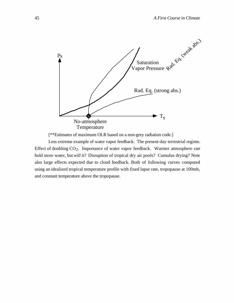
45 A First Course in Climate
Ts
psSaturation
Vapor Pressure Rad. E
q. (w
eak a
bs.)
Rad. Eq. (strong abs.)
No-atmosphereTemperature
[**Estimates of maximum OLR based on a non-grey radiation code.]
Less extreme example of water vapor feedback. The present-day terrestrial regime.
Effect of doubling CO2. Importance of water vapor feedback. Warmer atmosphere can
hold more water, but will it? Disruption of tropical dry air pools? Cumulus drying? Note
also large effects expected due to cloud feedback. Both of following curves computed
using an idealized tropical temperature profile with fixed lapse rate, tropopause at 100mb,
and constant temperature above the tropopause.
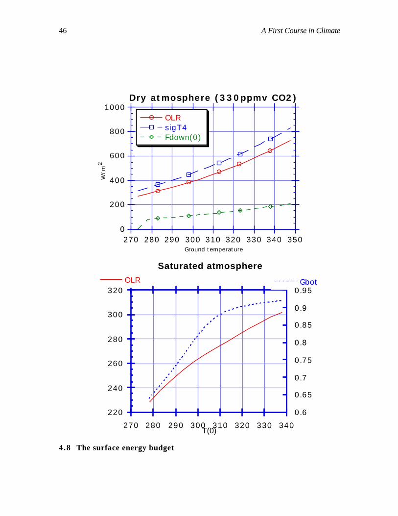
46 A First Course in Climate
0
200
400
600
800
1000
270
W/m
2
280 290 300 310 320 330 340 350Ground temperature
Dry atmosphere (330ppmv CO2)
OLRsigT4Fdown(0)
220
240
260
280
300
320
0.6
0.65
0.7
0.75
0.8
0.85
0.9
0.95
270 280 290 300 310 320 330 340T(0)
Saturated atmosphere
OLR Gbot
4.8 The surface energy budget
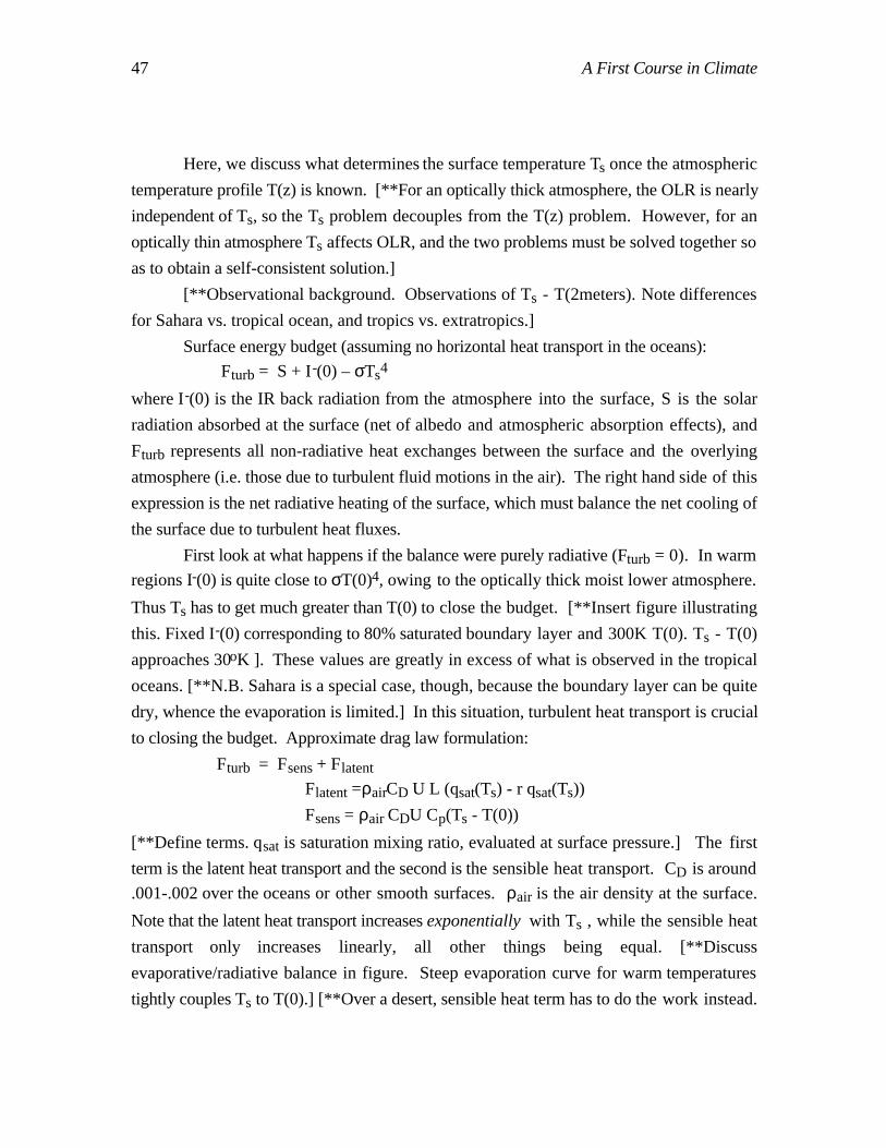
47 A First Course in Climate
Here, we discuss what determines the surface temperature Ts once the atmospheric
temperature profile T(z) is known. [**For an optically thick atmosphere, the OLR is nearly
independent of Ts, so the Ts problem decouples from the T(z) problem. However, for an
optically thin atmosphere Ts affects OLR, and the two problems must be solved together so
as to obtain a self-consistent solution.]
[**Observational background. Observations of Ts - T(2meters). Note differences
for Sahara vs. tropical ocean, and tropics vs. extratropics.]
Surface energy budget (assuming no horizontal heat transport in the oceans):
Fturb = S + I-(0) – σTs4
where I-(0) is the IR back radiation from the atmosphere into the surface, S is the solar
radiation absorbed at the surface (net of albedo and atmospheric absorption effects), and
Fturb represents all non-radiative heat exchanges between the surface and the overlying
atmosphere (i.e. those due to turbulent fluid motions in the air). The right hand side of this
expression is the net radiative heating of the surface, which must balance the net cooling of
the surface due to turbulent heat fluxes.
First look at what happens if the balance were purely radiative (Fturb = 0). In warm
regions I-(0) is quite close to σT(0)4, owing to the optically thick moist lower atmosphere.
Thus Ts has to get much greater than T(0) to close the budget. [**Insert figure illustrating
this. Fixed I-(0) corresponding to 80% saturated boundary layer and 300K T(0). Ts - T(0)
approaches 30oK ]. These values are greatly in excess of what is observed in the tropical
oceans. [**N.B. Sahara is a special case, though, because the boundary layer can be quite
dry, whence the evaporation is limited.] In this situation, turbulent heat transport is crucial
to closing the budget. Approximate drag law formulation:
Fturb = Fsens + Flatent
Flatent =ρairCD U L (qsat(Ts) - r qsat(Ts))
Fsens = ρair CDU Cp(Ts - T(0))
[**Define terms. qsat is saturation mixing ratio, evaluated at surface pressure.] The first
term is the latent heat transport and the second is the sensible heat transport. CD is around
.001-.002 over the oceans or other smooth surfaces. ρair is the air density at the surface.
Note that the latent heat transport increases exponentially with Ts , while the sensible heat
transport only increases linearly, all other things being equal. [**Discuss
evaporative/radiative balance in figure. Steep evaporation curve for warm temperatures
tightly couples Ts to T(0).] [**Over a desert, sensible heat term has to do the work instead.
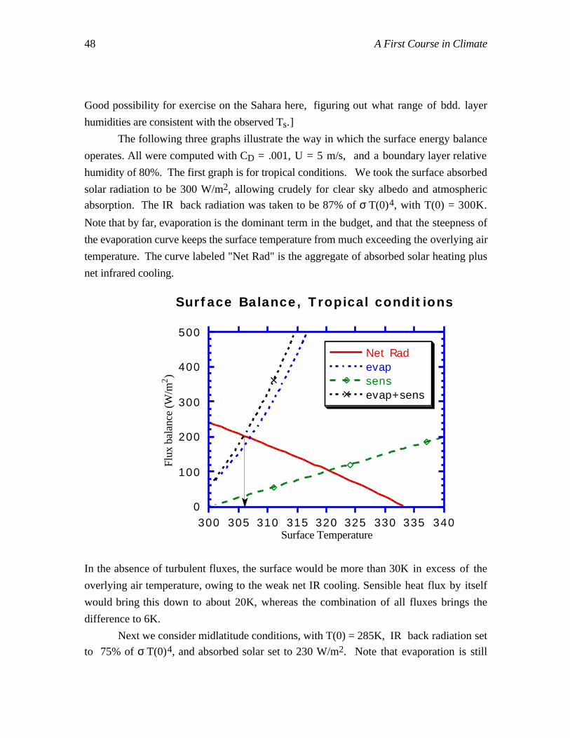
48 A First Course in Climate
Good possibility for exercise on the Sahara here, figuring out what range of bdd. layer
humidities are consistent with the observed Ts.]
The following three graphs illustrate the way in which the surface energy balance
operates. All were computed with CD = .001, U = 5 m/s, and a boundary layer relative
humidity of 80%. The first graph is for tropical conditions. We took the surface absorbed
solar radiation to be 300 W/m2, allowing crudely for clear sky albedo and atmospheric
absorption. The IR back radiation was taken to be 87% of σ T(0)4, with T(0) = 300K.
Note that by far, evaporation is the dominant term in the budget, and that the steepness of
the evaporation curve keeps the surface temperature from much exceeding the overlying air
temperature. The curve labeled "Net Rad" is the aggregate of absorbed solar heating plus
net infrared cooling.
0
100
200
300
400
500
Flux
bal
ance
(W/m
2 )
300 305 310 315 320 325 330 335 340Surface Temperature
Surface Balance, Tropical conditions
Net Radevapsensevap+sens
In the absence of turbulent fluxes, the surface would be more than 30K in excess of the
overlying air temperature, owing to the weak net IR cooling. Sensible heat flux by itself
would bring this down to about 20K, whereas the combination of all fluxes brings the
difference to 6K.
Next we consider midlatitude conditions, with T(0) = 285K, IR back radiation set
to 75% of σ T(0)4, and absorbed solar set to 230 W/m2. Note that evaporation is still
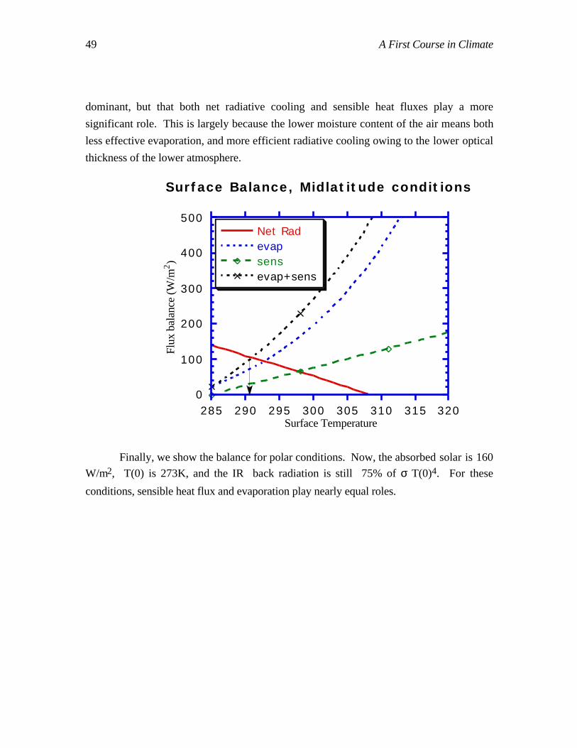
49 A First Course in Climate
dominant, but that both net radiative cooling and sensible heat fluxes play a more
significant role. This is largely because the lower moisture content of the air means both
less effective evaporation, and more efficient radiative cooling owing to the lower optical
thickness of the lower atmosphere.
0
100
200
300
400
500
Flux
bal
ance
(W/m
2 )
285 290 295 300 305 310 315 320Surface Temperature
Surface Balance, Midlatitude conditions
Net Radevapsensevap+sens
Finally, we show the balance for polar conditions. Now, the absorbed solar is 160
W/m2, T(0) is 273K, and the IR back radiation is still 75% of σ T(0)4. For these
conditions, sensible heat flux and evaporation play nearly equal roles.
50 A First Course in Climate
0
50
100
150
200
250Fl
ux b
alan
ce (W
/m2 )
300
273 279.8 286.5 293.3 300
Net Rad
Surface Temperature
Surface Balance, Polar conditions
evapsensevap+sens
Note that in all three cases, the fluxes conspire to keep the surface temperature to
within about 5K of the overlying air temperature. Compared to oceanic observations, this
value is generally too large. [**Give a map showing typical values. Main culprit in
overestimate is probably clouds. Clouds reduce the solar radiation absorbed at the surface,
but don't affect the IR back radiation much. Could also increase turbulent fluxes with a
larger CD or U.]
[**Analysis of "stiffness" of surface temperature, by linearized exchange
coefficients. Table of exchange coefficients at two temperatures.] At T=To,
krad = ddT σT4 = 4 σ To3
ksens=ddT Fsens = ρaCpCDU
Before we do the latent heat, note the approximate expression:
qsat = qsat(To) exp{ L
RwTo2 (T-To)}
so
klatent = ddT Flatent = ksens
L2
RwCpTo2 qsat(To)
51 A First Course in Climate
In the exchange coefficient for latent heat, the ratio appearing second has the value 156 at
To = 300K (when the condensible substance is water). It is not very sensitive to To. The
main temperature dependence comes through the exponential dependence of qsat on
temperature. qsat = 3.5 g/Kg at 273K, 6.2 g/Kg at 280K, 22.3 g/Kg at 300K, and 68.2
g/Kg at 320K.
The following table gives values of the exchange coefficients, in W/(m2K). Based
on Cd = .002, U=10m/s, and r = 100%.
To krad ksens klatent
280 5. 20. 20.
300 6. 20. 70.
[**When can the low layer air become decoupled from the air aloft? Tropical
boundary layer, and the trade inversion.]
4.7 Models of convective heat and moisture transport
"Just enough convection." A fascinating and wide-ranging subject. Refer to
Emanuel book for those wishing to pursue the matter in depth.
Dry incompressible convection. Scaling laws for heat flux in an infinitely thick
layer. Dynamics of ascending thermals. Summary of modern laboratory results.
Dry compressible convection.
Convection for a thermal penetrating a statically stable environment.
Moist convection. Classical entraining-plume models and stochastic mixing
models. Moist convective adjustment.
5. Seasonal, diurnal and latitudinal variations oftemperature5.1 Introduction
Geometry and astronomy. Geometric effects on sphere with no axis tilt, i.e. effect
of orientation of surface upon which radiation is incident.
Effect of axis tilt. Geometric effects vs. length-of-day effects. Have been doing
global average radiation balance -- assumes that response of system averages out inputs
over days, latitudes, etc. Some planets can do this, some can't. Calculation of
equatorial,noontime radiative equilibrium temperature on Earth. (Based on 1380 W/m2,
52 A First Course in Climate
even without Greenhouse effect this would be 395oK; at night, of course, it would fall to
absolute zero) Relative unimportance of eccentricity of Earth's orbit in seasonality (not
quite so with Mars, though!). Time scales for equilibration?. Compare to diurnal cycle on
Moon Mercury, which have no oceans or atmospheres. In lunar tropics, surface
temperature at local noon reaches 403oK. At midnight and dawn, lunar surface temperature
is -173oC. Temp changes penetrate only to about 50cm; below temp is constant at around
-30oC. Mercury: Mean surface temperature 350oC by day, -170oC by night.
5.2 Thermal inertia
Issue of thermal inertia. Thermal inertia for a mixed layer of fluid.ddt ρΗΑCpT = (F - σT4)A (2.3.1)
where H is the depth of the well-mixed layer, A is the area of the surface at the top of the
layer, ρ is the density of the substance making up the mixed layer (e.g. 1000 Kg/m3 for
water) and F is the incident radiation absorbed (or more generally the heat flux into the
surface from whatever sources. The factors of A cancel out, leaving the equationdTdt =
1
ρHCp (F - σT4) (2.3.1a)
which is now a closed first-order ordinary differential equation for T(t). In general,
F could be a function of time, but if F is constant it has the equilibrium solution Te, defined
by σTe4 = F. [**Linearization around Te. Radiative damping time, τ = ρHCp/(4σTe3).
Typical numbers.]
[**Simple mixed layer model of polar night cooling. Set F=0 in (2.3.1a) and let
the initial temperature be To. This somewhat exaggerates cooling because the actual heat
loss to space is less than σT4, owing to the greenhouse effect. In the dry polar regions,
this is not as serious a flaw as it would be in the moist tropical regions. Solution:]TTo
= ( τ/(t + τ) )1/3
where now τ = ρHCp/(3σTo3) , which is similar in form to the radiative damping time we
computed earlier, except it is now based on the initial temperature. For t<<τ, the
temperature drops linearly with time, but at large times, the temperature decays much more
slowly — namely, like (τ/t)1/3.
[**Review of diffusion equation. Characteristic scale Dt. Self-similar Gaussian
solution for evolution of initial spike.]
The diffusion coefficients for solids are typically very small. For ice near 0oC, D is
approximately .0114 cm2/s; the diffusive length scale corresponding to 1day is only 31
53 A First Course in Climate
cm., growing to 3.1 meters at 100 days; even after 100000 years, heat diffuses only to a
depth of 1.8 km (neglecting the effect of the slow creeping flow of the ice). Other solids
have similar or even lower diffusivities (Quartz, .044 cm2/sec, clay .015, organic matter
.001). The shallow penetration depth implies a rapid initial drop in surface temperature in
response to radiative cooling, with the rate of drop gradually decreasing as the thermal
influence taps the reservoir of heat at progressively greater depth.
[**Handwaving solution for surface temperature in terms of equivalent mixed
layer.] Qualitatively, we might expect the thermal behavior of a solid to behave like a
mixed-layer model with a time-dependent mixed layer depth given by H= Dt . Let's
substitute this in 2.3.1 and ignore the radiative cooling for the moment, assuming instead
that the flux F represents a constant cooling. Then the solution for the surface temperature
T(t) is
T = T0 + F
ρ DCpt
where To is the initial temperature (which comes in as an initial condition. Since F is
negative, this yields a steady reduction in temperature, which starts off infinitely steeply,
but is slower than linear over long times.
This solution may be obtained somewhat more rigorously in terms of a "broken
stick" approximation to the temperature profile. [**Discuss "broken stick solution. In fact,
it gives the rigorously correct asymptotic solution at long times.]
In the following we show numerical solutions for the actual diffusion equation
cooled from the surface, for the diffusivity of ice. The first figure gives the depth profile of
the cooling.
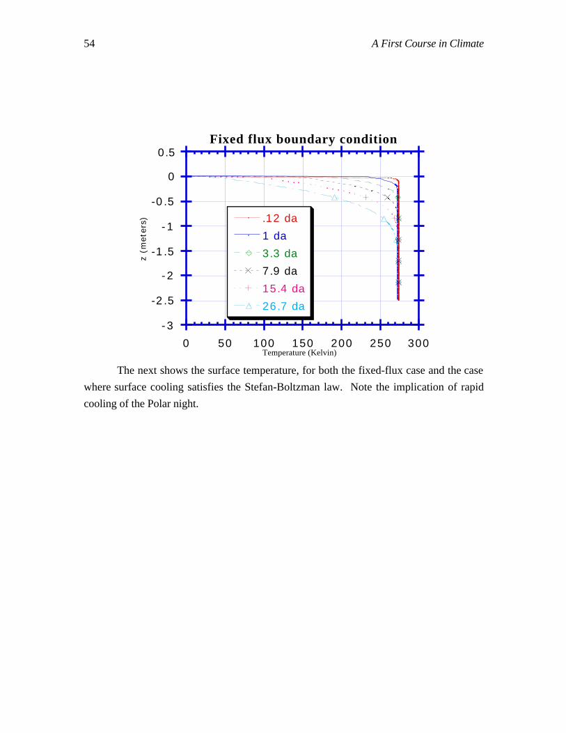
54 A First Course in Climate
0 50 100 150 200 250 300
-3
-2.5
-2
-1.5
-1
-0.5
0
0.5
Temperature (Kelvin)
z (m
eter
s)Fixed flux boundary condition
.12 da
1 da
3.3 da
7.9 da
15.4 da
26.7 da
The next shows the surface temperature, for both the fixed-flux case and the case
where surface cooling satisfies the Stefan-Boltzman law. Note the implication of rapid
cooling of the Polar night.
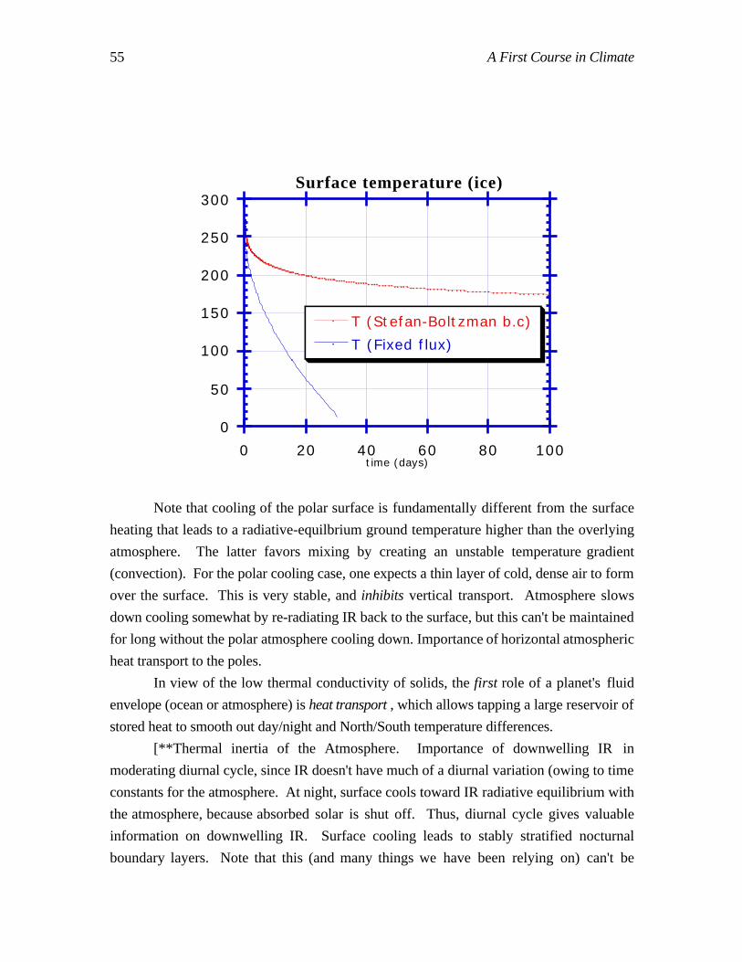
55 A First Course in Climate
0
50
100
150
200
250
300
0 20 40 60 80 100time (days)
Surface temperature (ice)
T (Stefan-Boltzman b.c)
T (Fixed flux)
Note that cooling of the polar surface is fundamentally different from the surface
heating that leads to a radiative-equilbrium ground temperature higher than the overlying
atmosphere. The latter favors mixing by creating an unstable temperature gradient
(convection). For the polar cooling case, one expects a thin layer of cold, dense air to form
over the surface. This is very stable, and inhibits vertical transport. Atmosphere slows
down cooling somewhat by re-radiating IR back to the surface, but this can't be maintained
for long without the polar atmosphere cooling down. Importance of horizontal atmospheric
heat transport to the poles.
In view of the low thermal conductivity of solids, the first role of a planet's fluid
envelope (ocean or atmosphere) is heat transport , which allows tapping a large reservoir of
stored heat to smooth out day/night and North/South temperature differences.
[**Thermal inertia of the Atmosphere. Importance of downwelling IR in
moderating diurnal cycle, since IR doesn't have much of a diurnal variation (owing to time
constants for the atmosphere. At night, surface cools toward IR radiative equilibrium with
the atmosphere, because absorbed solar is shut off. Thus, diurnal cycle gives valuable
information on downwelling IR. Surface cooling leads to stably stratified nocturnal
boundary layers. Note that this (and many things we have been relying on) can't be
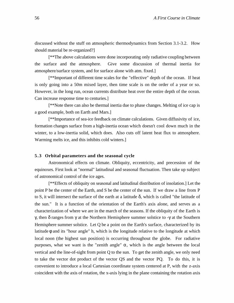
56 A First Course in Climate
discussed without the stuff on atmospheric thermodynamics from Section 3.1-3.2. How
should material be re-organized?]
[**The above calculations were done incorporating only radiative coupling between
the surface and the atmosphere. Give some discussion of thermal inertia for
atmosphere/surface system, and for surface alone with atm. fixed.]
[**Important of different time scales for the "effective" depth of the ocean. If heat
is only going into a 50m mixed layer, then time scale is on the order of a year or so.
However, in the long run, ocean currents distribute heat over the entire depth of the ocean.
Can increase response time to centuries.]
[**Note there can also be thermal inertia due to phase changes. Melting of ice cap is
a good example, both on Earth and Mars.]
[**Importance of sea-ice feedback on climate calculations. Given diffusivity of ice,
formation changes surface from a high-inertia ocean which doesn't cool down much in the
winter, to a low-inertia solid, which does. Also cuts off latent heat flux to atmosphere.
Warming melts ice, and this inhibits cold winters.]
5.3 Orbital parameters and the seasonal cycle
Astronomical effects on climate. Obliquity, eccentricity, and precession of the
equinoxes. First look at "normal" latitudinal and seasonal fluctuation. Then take up subject
of astronomical control of the ice ages.
[**Effects of obliquity on seasonal and latitudinal distribution of insolation.] Let the
point P be the center of the Earth, and S be the center of the sun. If we draw a line from P
to S, it will intersect the surface of the earth at a latitude δ, which is called "the latitude of
the sun." It is a function of the orientation of the Earth's axis alone, and serves as a
characterization of where we are in the march of the seasons. If the obliquity of the Earth is
γ, then δ ranges from γ at the Northern Hemisphere summer solstice to -γ at the Southern
Hemisphere summer solstice. Let Q be a point on the Earth's surface, characterized by its
latitude φ and its "hour angle" h, which is the longitude relative to the longitude at which
local noon (the highest sun position) is occurring throughout the globe. For radiative
purposes, what we want is the "zenith angle" α, which is the angle between the local
vertical and the line-of-sight from point Q to the sun. To get the zenith angle, we only need
to take the vector dot product of the vector QS and the vector PQ. To do this, it is
convenient to introduce a local Cartesian coordinate system centered at P, with the z-axis
coincident with the axis of rotation, the x-axis lying in the plane containing the rotation axis
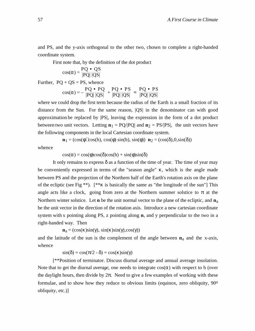
57 A First Course in Climate
and PS, and the y-axis orthogonal to the other two, chosen to complete a right-handed
coordinate system.
First note that, by the definition of the dot product
cos(α) = PQ • QS|PQ| |QS|
Further, PQ + QS = PS, whence
cos(α) = – PQ • PQ|PQ| |QS| +
PQ • PS|PQ| |QS| ≈
PQ • PS|PQ| |QS|
where we could drop the first term because the radius of the Earth is a small fraction of its
distance from the Sun. For the same reason, |QS| in the denominator can with good
approximation be replaced by |PS|, leaving the expression in the form of a dot product
between two unit vectors. Letting n1 = PQ/|PQ| and n2 = PS/|PS|, the unit vectors have
the following components in the local Cartesian coordinate system.
n1 = (cos(φ) cos(h), cos(φ) sin(h), sin(φ)) n2 = (cos(δ),0,sin(δ))
whence
cos(α) = cos(φ)cos(δ)cos(h) + sin(φ)sin(δ)
It only remains to express δ as a function of the time of year. The time of year may
be conveniently expressed in terms of the "season angle" κ, which is the angle made
between PS and the projection of the Northern half of the Earth's rotation axis on the plane
of the ecliptic (see Fig **). [**κ is basically the same as "the longitude of the sun"] This
angle acts like a clock, going from zero at the Northern summer solstice to π at the
Northern winter solstice. Let n be the unit normal vector to the plane of the ecliptic, and na
be the unit vector in the direction of the rotation axis. Introduce a new cartesian coordinate
system with x pointing along PS, z pointing along n, and y perpendicular to the two in a
right-handed way. Then
na = (cos(κ)sin(γ), sin(κ)sin(γ),cos(γ))
and the latitude of the sun is the complement of the angle between na and the x-axis,
whence
sin(δ) = cos(π/2 - δ) = cos(κ)sin(γ)
[**Position of terminator. Discuss diurnal average and annual average insolation.
Note that to get the diurnal average, one needs to integrate cos(α) with respect to h (over
the daylight hours, then divide by 2π. Need to give a few examples of working with these
formulae, and to show how they reduce to obvious limits (equinox, zero obliquity, 90o
obliquity, etc.)]
58 A First Course in Climate
The following contour plot shows the flux factor f as a function of latitude and
season, with the latitude being the vertical axis and the season being horizontal. f is defined
such that the diurnal mean flux received at the specified latitude circle is Lf watts/m2, where
L is the solar constant. It has been computed using the present value of the obliquity.
0.04
0.280.28
0.12
0.20
0.32
0.39
[**Discussion. Large polar fluctuations. Polar hotspot in summer, owing to long polar
day. No radiation at all in polar night. Importance of thermal inertia in midlatitude and
polar seasonal cycle.] The following graph illustrates this point dramatically. Here, we
have computed the radiative equilibrium temperature for the solar flux computed at the
solstice. Results are plotted for the Norther Hemisphere Summer solstice, but the Northern
Winter results may be obtained by simply flipping the plot about the equator. We show
results for a case with no atmosphere and zero albedo, and also for a case with an
atmosphere of bulk emissivity 1, and an albedo of 30%.
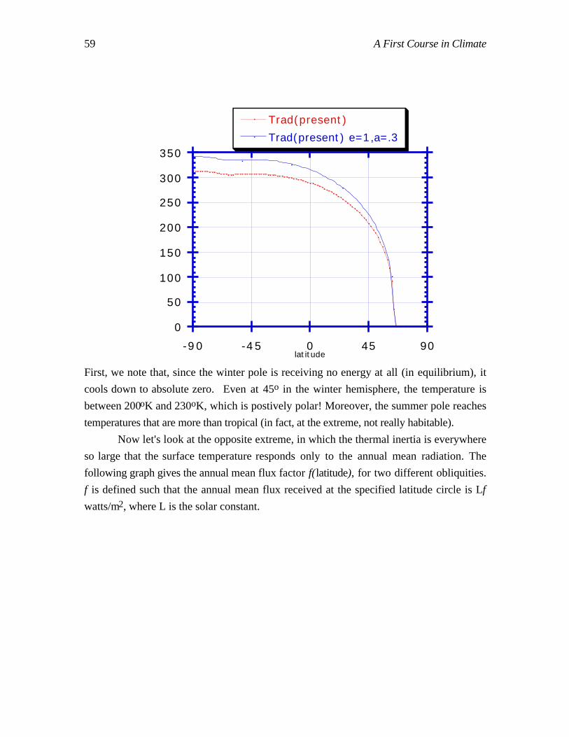
59 A First Course in Climate
0
50
100
150
200
250
300
350
-90 -45 0 45 90latitude
Trad(present)
Trad(present) e=1,a=.3
First, we note that, since the winter pole is receiving no energy at all (in equilibrium), it
cools down to absolute zero. Even at 45o in the winter hemisphere, the temperature is
between 200oK and 230oK, which is postively polar! Moreover, the summer pole reaches
temperatures that are more than tropical (in fact, at the extreme, not really habitable).
Now let's look at the opposite extreme, in which the thermal inertia is everywhere
so large that the surface temperature responds only to the annual mean radiation. The
following graph gives the annual mean flux factor f(latitude), for two different obliquities.
f is defined such that the annual mean flux received at the specified latitude circle is Lf
watts/m2, where L is the solar constant.
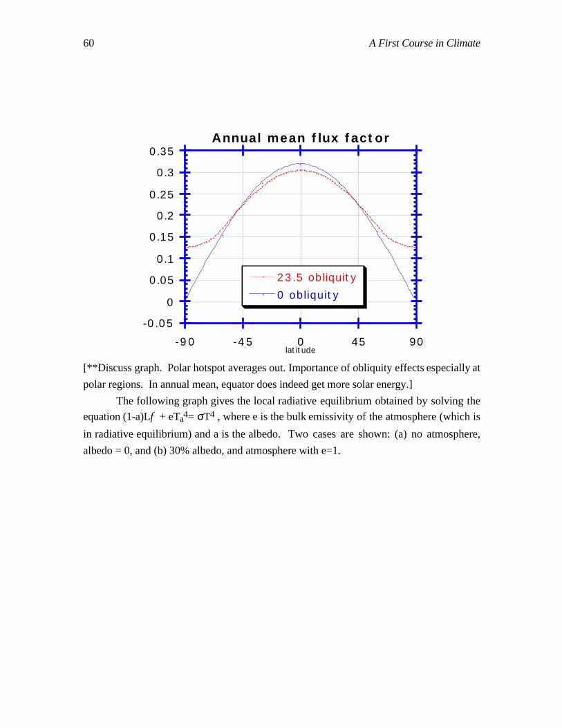
60 A First Course in Climate
-0.05
0
0.05
0.1
0.15
0.2
0.25
0.3
0.35
-90 -45 0 45 90latitude
Annual mean flux factor
23.5 obliquity
0 obliquity
[**Discuss graph. Polar hotspot averages out. Importance of obliquity effects especially at
polar regions. In annual mean, equator does indeed get more solar energy.]
The following graph gives the local radiative equilibrium obtained by solving the
equation (1-a)Lf + eTa4= σT4 , where e is the bulk emissivity of the atmosphere (which is
in radiative equilibrium) and a is the albedo. Two cases are shown: (a) no atmosphere,
albedo = 0, and (b) 30% albedo, and atmosphere with e=1.
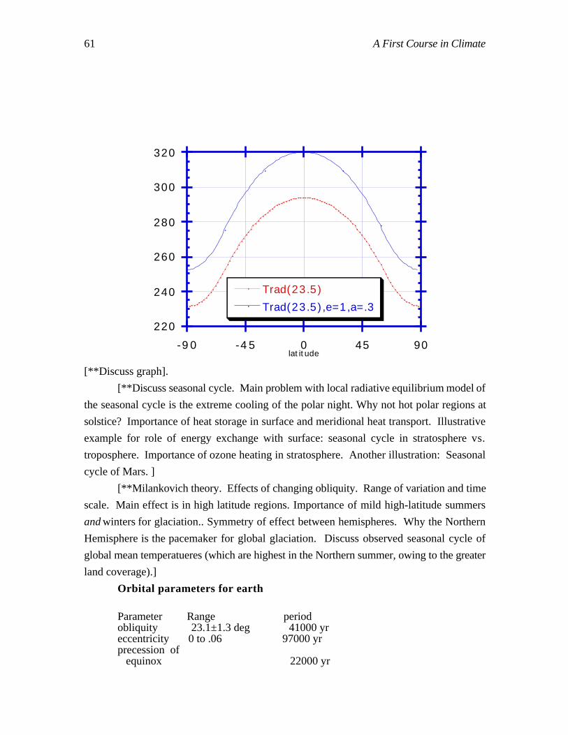
61 A First Course in Climate
220
240
260
280
300
320
-90 -45 0 45 90latitude
Trad(23.5)
Trad(23.5),e=1,a=.3
[**Discuss graph].
[**Discuss seasonal cycle. Main problem with local radiative equilibrium model of
the seasonal cycle is the extreme cooling of the polar night. Why not hot polar regions at
solstice? Importance of heat storage in surface and meridional heat transport. Illustrative
example for role of energy exchange with surface: seasonal cycle in stratosphere vs.
troposphere. Importance of ozone heating in stratosphere. Another illustration: Seasonal
cycle of Mars. ]
[**Milankovich theory. Effects of changing obliquity. Range of variation and time
scale. Main effect is in high latitude regions. Importance of mild high-latitude summers
and winters for glaciation.. Symmetry of effect between hemispheres. Why the Northern
Hemisphere is the pacemaker for global glaciation. Discuss observed seasonal cycle of
global mean temperatueres (which are highest in the Northern summer, owing to the greater
land coverage).]
Orbital parameters for earth
Parameter Range periodobliquity 23.1±1.3 deg 41000 yreccentricity 0 to .06 97000 yrprecession of equinox 22000 yr
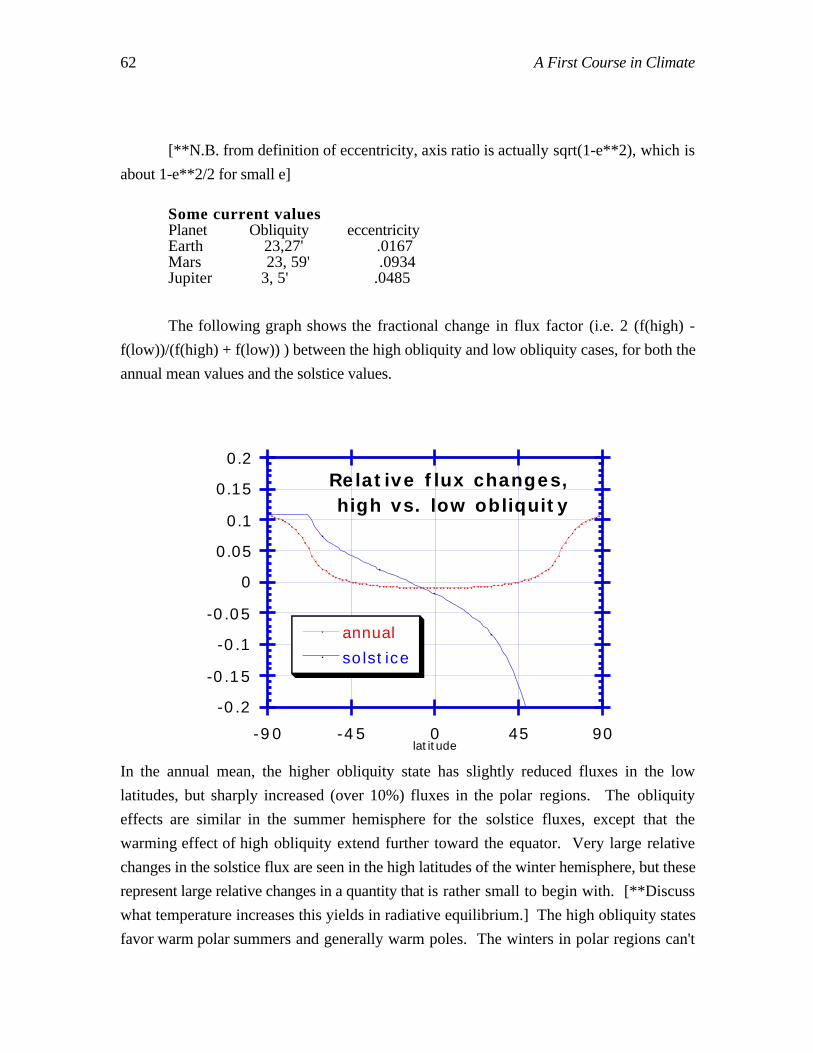
62 A First Course in Climate
[**N.B. from definition of eccentricity, axis ratio is actually sqrt(1-e**2), which is
about 1-e**2/2 for small e]
Some current valuesPlanet Obliquity eccentricityEarth 23,27' .0167Mars 23, 59' .0934Jupiter 3, 5' .0485
The following graph shows the fractional change in flux factor (i.e. 2 (f(high) -
f(low))/(f(high) + f(low)) ) between the high obliquity and low obliquity cases, for both the
annual mean values and the solstice values.
-0.2
-0.15
-0.1
-0.05
0
0.05
0.1
0.15
0.2
-90latitude
Relative flux changes, high vs. low obliquity
annual
solstice
-45 0 45 90
In the annual mean, the higher obliquity state has slightly reduced fluxes in the low
latitudes, but sharply increased (over 10%) fluxes in the polar regions. The obliquity
effects are similar in the summer hemisphere for the solstice fluxes, except that the
warming effect of high obliquity extend further toward the equator. Very large relative
changes in the solstice flux are seen in the high latitudes of the winter hemisphere, but these
represent large relative changes in a quantity that is rather small to begin with. [**Discuss
what temperature increases this yields in radiative equilibrium.] The high obliquity states
favor warm polar summers and generally warm poles. The winters in polar regions can't
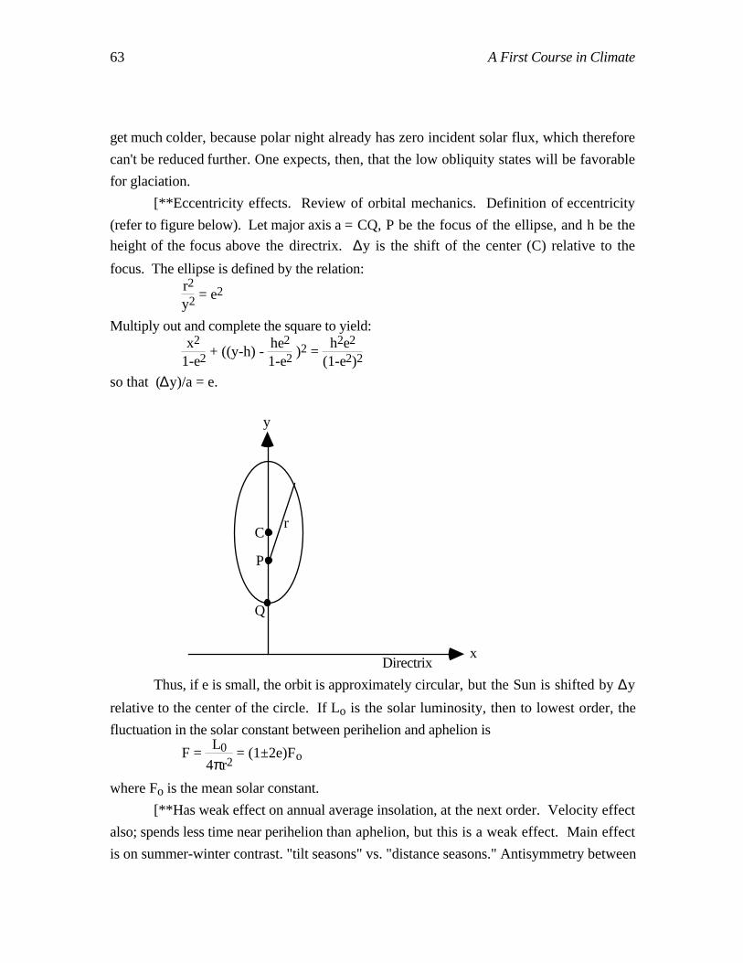
63 A First Course in Climate
get much colder, because polar night already has zero incident solar flux, which therefore
can't be reduced further. One expects, then, that the low obliquity states will be favorable
for glaciation.
[**Eccentricity effects. Review of orbital mechanics. Definition of eccentricity
(refer to figure below). Let major axis a = CQ, P be the focus of the ellipse, and h be the
height of the focus above the directrix. ∆y is the shift of the center (C) relative to the
focus. The ellipse is defined by the relation:r2
y2 = e2
Multiply out and complete the square to yield:x2
1-e2 + ((y-h) - he2
1-e2 )2 = h2e2
(1-e2)2
so that (∆y)/a = e.
Directrixx
y
P
C
Q
r
Thus, if e is small, the orbit is approximately circular, but the Sun is shifted by ∆y
relative to the center of the circle. If Lo is the solar luminosity, then to lowest order, the
fluctuation in the solar constant between perihelion and aphelion is
F = L0
4πr2 = (1±2e)Fo
where Fo is the mean solar constant.
[**Has weak effect on annual average insolation, at the next order. Velocity effect
also; spends less time near perihelion than aphelion, but this is a weak effect. Main effect
is on summer-winter contrast. "tilt seasons" vs. "distance seasons." Antisymmetry between
64 A First Course in Climate
hemispheres in eccentricity effect. Note also, eccentricity signal is the strongest periodicity
in the ice record, but is a relatively weak radiative effect. Conflict with historical data: In
Pleistocene, Northern Hemisphere is the pacemaker for ice ages globally. Present evidence
for climatic effect of eccentricity: N-S asymmetry of seasonal cycle on Mars.]
[**Effect of precession of perihelion (important only in conjunction with seasonal
cycle.). Split precessional cycles, and effects on the tropics. Bond cycles, Dansgaard-
Oeschgar events. Important example of the precession signal: the Holocene optimum.]
5.4 Ice albedo feedback
6. Afterword to Volume I[**Philosophical remarks on climate. CO2, water, and life on earth.]
[**Dynamics. Role of rotation of planets.]
7. Fluid mechanics: Fundamentals[**Compressible PE equations on a sphere, in pressure coordinates. Rotating
reference frame. Isentropic coordinates. Ertel PV conservation. One layer (shallow-water)
and two-layer variants. ]
8. The Tropics, part I: Hadley circulations8.1 Diabatic heating and vertical velocity
Role of water in energy exchange between surface and atmosphere: Solar energy
absorbed in sea evaporates water, which goes into atmosphere and releases energy at
higher levels and other latitudes when it condenses.
Steady state balance. Heating and ascent
Role of radiative cooling in limiting ascent
8.2 Mass continuity relation.
Mean meridional circulation
ITCZ
8.3 Angular momentum conservation. Trade winds
8.4 Momentum budget (Bernoulli equation)
Pressure forces determine why the tropics cannot persist in a state of local radiative-
convective equilibrium. If it did, tropical low would lead to low pressure, and air would
rush in, creating the Hadley circulation. Because the upper level outflow must fight an
65 A First Course in Climate
adverse pressure gradient, the pressure forces also act to limit the meridional extent of the
Hadley cell (but not enough to account for the observations, evidently).
Observations show asymmetry of Hadley cell descending branch between the
hemispheres. The strong descent is always in the winter hemisphere (and is very sharply
defined, contradicting the picture of gentle descent due to radiative cooling). Why?
8.5 A two-box model of the tropical circulation
8.6 The Held/Hou model.
8. The Tropics, part II: Zonally asymmetricmotions8.1 Basic wave concepts
[**Dispersion relation, phase velocity, group velocity, ray paths.]
8.2 Equatorial beta-plane waves
8 .3 The Walker circulation
66 A First Course in Climate
9. Fundamentals of midlatitude dynamics9.1 Geostrophic balance
9 .2 Quasigeostrophic theory: Shallow water case
9 .3 Quasigeostrophic theory: General case
Geostrophy. Basic concepts QG theory.
9.4 Fundamental conservation laws
[**Pseudomomentum and pseudo energy. Things that will be of importance both
for wave theory and for stability theory.]
9.5 The Ekman layer
10. Rossby waves10.1 Free wave dispersion relation
10.2 Free waves in vertical shear
10.3 Forced Stationary waves
10.4 Ray tracing theory. Wave trains
11. Synoptic scale transient eddies[**Basically the stuff in my Ann. Rev. review article.]
[**Perhaps we can also include some numerical methods for stability theory here.]
12. General circulation models[**This section introduces numerical concepts needed to do modeling on a sphere.
It leads up to discussions of the behavior of the models, and their general use in addressing
climate problems.]
[**It might actually be better to have this part earlier (before Chapter 7). This
would permit us to use the GCM's to illustrate basic phenomena (like synoptic eddies) as
they come along. The main question is how to arrange presentation of the basic physics
(e.g. the Rossby wave chapter) vs. the presentation of nonlinear transient models, which
can be used to illustrate the concepts in a more realistic context.]
12.1 Shallow water model on a sphere
67 A First Course in Climate
12.2 A two layer primitive equation model
12.3 A dry multi-level GCM
12.4 Multi-level GCM with a hydrological cycle
68 A First Course in Climate
A1 A brief handbook of atmospheric physicsThermodynamics
1mb = 100 Pascals = 100 Kg/(m sec2)
Tabs = -273.15 oC
p = ρ R T, where T is in oK and R is the gas constant for the gas in question. R is
related to the universal gas constant R* by the relation R = R*/M, where M is the molecular
weight of the gas.
R* = 8314.3 Joule/(oK kmol)
Mwater = 18.016, so Rvapor = 461.
Mdry air = 28.97, so Rdry air = 287.
MCO2 = 44, so RCO2 = 188.96
Specific heats cv = (dq/dT)|ρ=const = (du/dt)|ρ=const, where u=u(T) is the internal
energy of the gas. Let specific volume α = 1/ρ. Since dq = du + pdα=cvdT + pdα =
(cv+R)dT -αdp we have cp = cv + R = (dq/dT)|p=const.
Dry air: cv = 717 J/(o Kg), cp = 1004 J/(o Kg) , R/cp = 2/7
CO2: cp = 820 at 0 oC, about 1000 at 400 oC.
Water vapor: cv = 1463, cp = 1952
Liquid water: cv = 4218 (approximately incompressible, i.e. cv = cp)
Water ice: cv = 2106 (approximately incompressible, i.e. cv = cp)
Water: Latent heat of melting L = 3.34 105 J/Kg at standard temperature and
pressure. Latent heat of vaporization L = 2.5 106 J/Kg at 0oC ( 2.25 106 at 100oC).
Critical point (p,T,ρ) = ( 22.064 MegaPascals, 647.15 oK, 3110 Kg/m3)
Clausius-Clapeyron relation: des/dT = L/((α2 - α1)T), where es is saturation vapor
pressure and α2 is the specific volume of the vapor phase. If L = const. and α2>>α1, then
es = e∞ exp(-L/RT)
where R is the gas constant for the pure vapor in question (e.g. the gas constant for pure
water vapor, in the case of water). For water not too far from STP, e∞ = 2.6 1011 Pa and
L/R = 5423 oK .
For water, es = 6.108mb at 0oC, and .189 mb at -40oC.
69 A First Course in Climate
If the water mixing ratio in air is small, then the mass mixing ratio is given
approximately by ws = es/p. e.g. ws = 3.5 g/Kg at 0oC for p = 1000mb.
1 Megaton TNT-equivalent = 4.2 1022 ergs = 4.2 1012 Joules.
1 Joule = .000238662 Kg-cal
1 g-cal = 4.1860 Joule
Radiationσ(Stefan-Boltzman constant) = 5.6696 10-8 Watt/(m2 oK4)
Solar flux L at mean radius of Earth's orbit = 1370 W/m2
Fossil Fuel Facts
1 Joule = .000948608 BTU
Petroleum facts:
1 Barrel Petroleum = 158.98 Liter
Gasoline combustion releases 5.253 106 BTU/barrel
Motor gasoline: 19.5 Million Metric Tons Carbon per Quadrillion BTU
[**Carbon emission per liter.]
n-octane is C8H18; heat of combustion = 1303 Kg-cal/gram-mole
n-Hexane is C6H24; heat of combustion = 995 Kg-cal/gram-mole
Coal facts:
Natural gas facts:
Earth constants
Radius of Earth = 6.37 106m
g = acceleration of gravity = 9.8 m/sec2
ωday = 7.292 10-5 radians/sec
mean distance from Sun = 1.5 1011 m
Mars constants
Radius = 3.394 106 m
g = acceleration of gravity = 3.72 m/s2
ωday = 7.078 10-5 radians/sec
mean distance from Sun =
70 A First Course in Climate
References
Bloggs. 19xx: Title. J. Fluid Mech nnn ,xx-xx.

2 A First Course in Climate
Notes for book with IsaacWith all the basic climate stuff normally included in 232, the project begins to
become unwieldy. Also, there may be too much overlap of the introductory material with
Hartmann's book. I suggest that the book with Isaac concentrate on the more dynamical
end (Sections 6 and onward), though keeping a good emphasis on application to real data
and providing the readers with working source code for models. Perhaps at some later
point I can write a "climate primer" companion volume with consistent notation.
Notes for revision[**Following can be used as outline for introductory GFD course, GFD I.]
1. Basic principals of fluid dynamics
1 .1 . What is a fluid and how is it characterized?
1.2. Deriving the equations of motion
Material (comoving) derivatives
Pressure Force
2D Incompressible flow2D equations of motion. Incompressibility constraint ρ= const., ∇.u = 0.
Diagnostic equation for pressure. Vorticity equation. Interpretation of vorticity
(circulation). Streamfunctions. Poisson equation for vorticity in terms of streamfunction.
1 .3 . Fluid dynamics in a rotating reference frame
Review of particle dynamics in rotating frame
Hockey puck on carousel. Centrifugal "force". Coriolis "force". Inertial circles.
3D momentum equations in a rotating frame
Rapidly rotating limit: Rossby numbers and the Geostrophic approximation
2D special case. Unstratified special case (Taylor-Proudman).
Geostrophic flow in a spherical shell