A Finite-state Machine for Accommodating Unexpected Large

Ground Height Variations in Bipedal Robot Walking

Hae-Won Park, Alireza Ramezani, and J.W. Grizzle

Abstract—This paper presents a feedback controller thatallows MABEL, a kneed planar bipedal robot with 1 m-long legs,to accommodate terrain that presents large unexpected increasesand decreases in height. The robot is provided informationon neither where the change in terrain height occurs, nor byhow much. A finite-state machine is designed that managestransitions among controllers for flat-ground walking, stepping-up and down, and a trip reflex. If the robot completes a step, thedepth of a step-down or height of a step-up can be immediatelyestimated at impact from the lengths of the legs and the anglesof the robot’s joints. The change in height can be used toinvoke a proper control response. On the other hand, if theswing leg impacts an obstacle during a step, or has a prematureimpact with the ground, a trip reflex is triggered on the basis ofspecially designed contact switches on the robot’s shins, contactswitches on the end of each leg, and the current configurationof the robot. The design of each control mode and the transitionconditions among them are presented. The paper concludes withexperimental results of MABEL (blindly) accommodating varioustypes of platforms, including ascent of a 12.5 cm high platform,stepping-off an 18.5 cm high platform, and walking over aplatform with multiple ascending and descending steps.

I. INTRODUCTION

Bipedal locomotion has attracted attention for its potential

ability, superior when compared to wheeled locomotion, to

overcome rough terrain or environments with discontinuous

supports. Existing bipedal robots, however, can only deal with

small unknown variations in ground height. Ground height

variations exceeding a few centimeters must be known a priori

and require carefully planned maneuvers to overcome them.

Two major avenues of research are currently being pur-

sued to quantify and improve the ability of a bipedal ma-

chine to walk over uneven terrain. A stochastic model of

ground variation is being investigated in [1], [2], [3] for low-

dimensional dynamical systems such as the rimless wheel and

the compass bipedal walker. The mean first-passage time to

the fallen absorbing state is used to assess the robustness of

a gait. This metric captures the expected time that a robot

can walk before falling down, measured in units of number

of steps. Numerical dynamic programming is applied to a

discretized representation of the dynamics to maximize the

mean first-passage time. In [4], [5], [6], the gait sensitivity

norm, defined as the H2 norm of the system’s state when

the input is ground-height variation, is introduced to quantify

the ability of a bipedal robot to handle changes in ground

H.-W. Park and A. Ramezani are with the Mechanical EngineeringDepartment, University of Michigan, Ann Arbor, MI, 48109-2125, USA,parkhw@umich.edu

J. W. Grizzle is with the Control Systems Laboratory, Electrical Engineeringand Computer Science Department, University of Michigan, Ann Arbor, MI48109-2122, USA.

This work is supported in part by NSF grant ECS-909300 and in part byDARPA Contract W91CRB-11-1-0002.

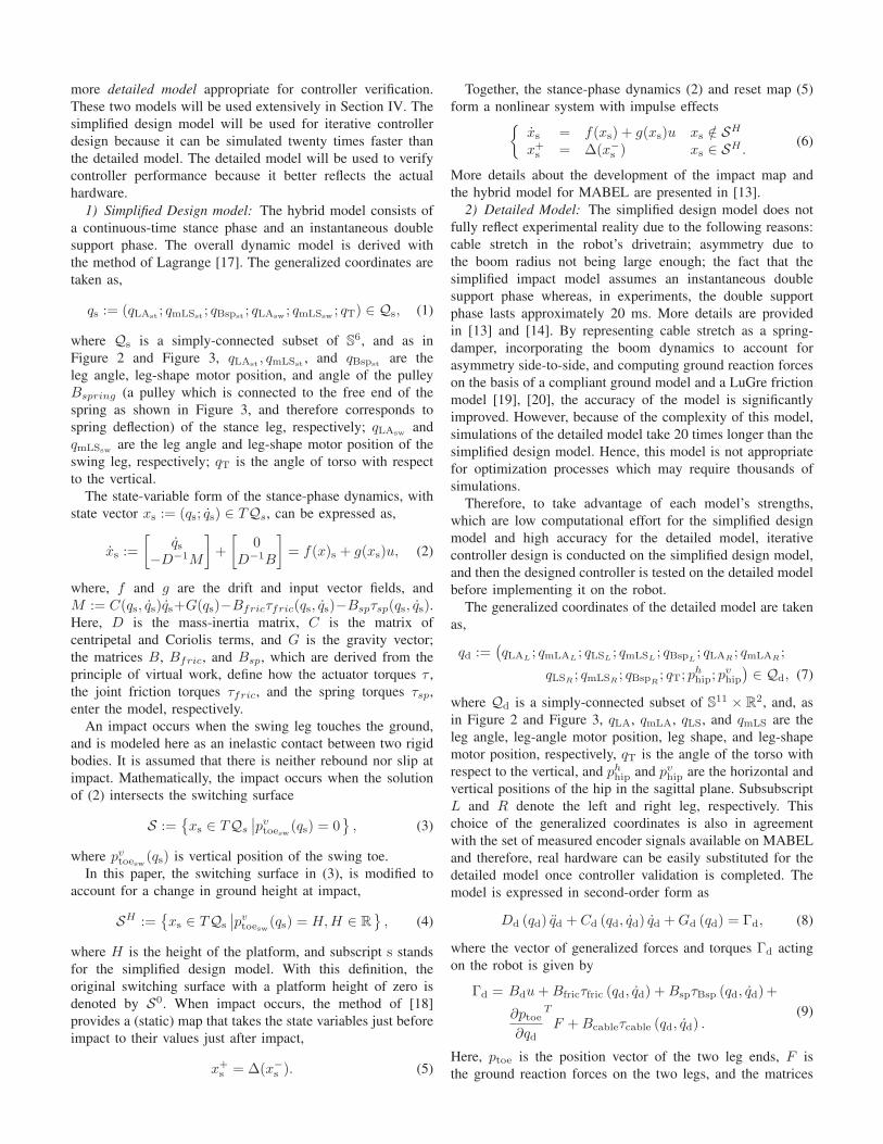
Fig. 1: MABEL, a planar testbed for bipedal locomotion, is

shown traversing a platform with 10.5 cm and 8 cm steps.

height. Particular attention is given to a “step-down test”,

where the ground profile consists of a flat section, followed by

an abrupt decrease in height, followed again by a flat section

of ground. These references use the gait sensitivity norm to

assess the improvement in disturbance rejection when swing-

leg retraction speed at the end of the step is varied [5].

Along with the search for the best quantity to measure

the robustness of bipedal walking to ground variation, several

control design approaches for walking over uneven ground

have been proposed in the literature. The work presented in [7],

[8] begins with the computation of a transverse linearization

around the desired trajectories; specifically, the transverse

linearization is a linear system with linearized impulse effects

which locally represents the original transversal dynamics

of a target trajectory. Next, a receding-horizon controller

is designed to exponentially stabilize the linear impulsive

system. The designed controller has been verified by a walking

experiment [7] over uneven ground where the height varied by

steps of 2.0 cm. A neural network was tuned to accommodate

irregular surfaces in [9]. The algorithm was tested on the robot

Rabbit, whose legs are 80 cm long, resulting in 1.5 cm ground-

height variations being accommodated.

A sensory reflex-based control strategy has been consid-

ered for bipedal walking [10] and for running over uneven

ground [11]. In response to various types of disturbance, such

as tripping and slipping [11], or step-down and step-up [10],

a separately designed reflex controller is activated to attenuate

the effects of the disturbances. The sensory reflex control

proposed in [10] was tested to accommodate obstacles 1.0 cm

in height, while a reflex strategy in [11] was verified only in

simulation to the best knowledge of the authors.

While important progress is being made on walking over

uneven ground, significant restrictions still remain. The exper-

imental work in [4], [5], [6], [9], [7] and [10] accommodates

only obstacles that are less than 6% of leg length, a value that

is unrealistically small when compared to common obstacles

(a)

−qT

qLA

qLS

VirtualCompliant Leg −θs

(b)

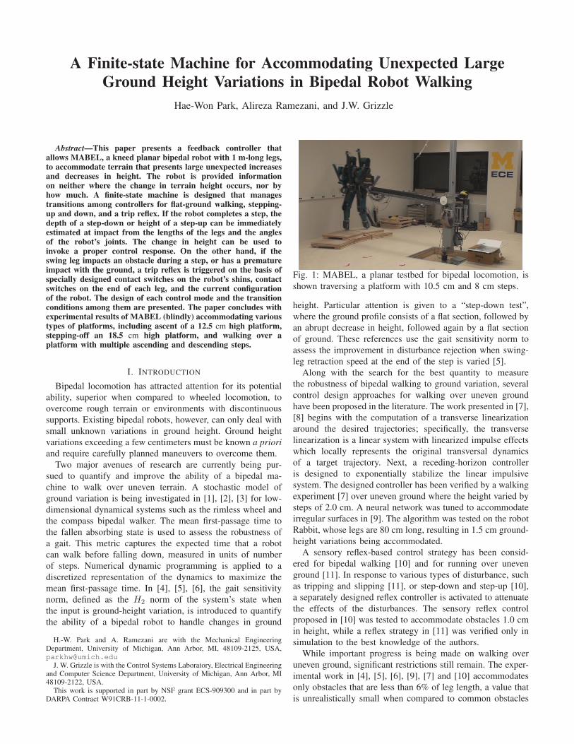
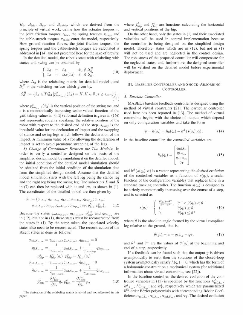
Fig. 2: (a) MABEL is shown with the switch in front of the

shin that is used to detect contact with obstacles. The robot

is planar, with a boom providing stabilization in the frontal

plane. The robot weighs 65 kg and is 1 m at the hip. (b) The

virtual compliant leg created by the drivetrain through a set

of differentials.

in everyday life, such as the height of steps in a building or

the curb height of a sidewalk on a city street.

In this paper, we propose a new control policy for the planar

bipedal robot MABEL [12], which weighs 65 kg and has

1 m-long legs. The control policy allows MABEL to traverse

various ground profiles, including ascent of a stair with a

height of 12.5 cm (12.5% of the leg length), step-down from

a platform with a height of 18.5 cm (18.5% of the leg length),

and walking over constructed platforms which consist of steps

with heights of 10.5 cm and 8.0 cm (see Figure 1), without

falling. The robot is provided information on neither where

the change in height occurs, nor by how much.

The remainder of the paper is organized as follows. Sec-

tion II describes the general features of MABEL’s morphology,

and summarizes two mathematical models for a walking gait.

Section III provides the design of the baseline controller

reported in [13] and an initial step-down experiment reported

in [14]. Individual control designs to accommodate various

types of obstacles including step-down, step-up, and tripping

are presented in Section IV. Section V introduces a finite-state

machine to manage the transitions among these controllers.

In Section VI, the overall controller is verified on a detailed

simulation model reported in [14]. Experimental results of

the new controller are provided in Section VII. Finally, Sec-

tion VIII provides concluding remarks and briefly discusses

future research plans.

II. HARDWARE AND MATHEMATICAL MODEL OF MABEL

This section briefly introduces MABEL, the robot used to

test the proposed finite-state machine, and two mathematical

models for control law design and verification. This material

is based primarily on [13], [12], [14].

A. Description of MABEL’s hardware

MABEL is a planar bipedal robot comprised of five rigid

links assembled to form a torso and two legs with knees. As

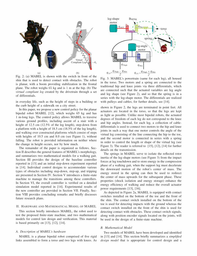
Bspring

qmLS

leg-shape

motor

torso

leg-angle

motor

qThigh qShin

qLS

−=qThigh qShin

2=qLA

qThigh qShin

2+

Bspring

spring

qBsp

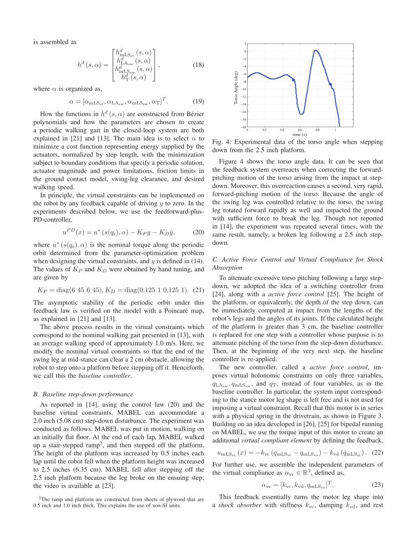
Fig. 3: MABEL’s powertrain (same for each leg), all housed

in the torso. Two motors and a spring are connected to the

traditional hip and knee joints via three differentials, which

are connected such that the actuated variables are leg angle

and leg shape (see Figure 2), and so that the spring is in a

series with the leg-shape motor. The differentials are realized

with pulleys and cables; for further details, see [14].

shown in Figure 2, the legs are terminated in point feet. All

actuators are located in the torso, so that the legs are kept

as light as possible. Unlike most bipedal robots, the actuated

degrees of freedom of each leg do not correspond to the knee

and hip angles. Instead, for each leg, a collection of cable-

differentials is used to connect two motors to the hip and knee

joints in such a way that one motor controls the angle of the

virtual leg consisting of the line connecting the hip to the toe,

and the second motor is connected in series with a spring

in order to control the length or shape of the virtual leg (see

Figure 3). The reader is referred to [15], [12], [14] for further

details on the transmission.

The springs in MABEL serve to isolate the reflected rotor

inertia of the leg-shape motors (see Figure 3) from the impact

forces at leg touchdown and to store energy in the compression

phase of a walking gait, when the support leg must decelerate

the downward motion of the robot’s center of mass. The

energy stored in the spring can then be used to redirect

the center of mass upwards for the subsequent phase. These

properties (shock isolation and energy storage) enhance the

energy efficiency of walking and reduce the overall actuator

power requirements [13], [16].

As depicted in Figure 2a, MABEL is equipped with contact

switches installed on the bottom of the toe and the front of

the shin. The contact switch installed on the bottom of the

toe is used for detecting impacts with the ground whereas the

contact switch installed on the front of the shin is used for

detecting contact with obstacles. These contact switch signals,

along with position encoder signals located on the joints, will

be used in the design of a finite-state machine.

B. Mathematical Model

Two models of MABEL have been developed and identified

in [13] and [14]. This section briefly summarizes a simplified

design model that is appropriate for control design and a

more detailed model appropriate for controller verification.

These two models will be used extensively in Section IV. The

simplified design model will be used for iterative controller

design because it can be simulated twenty times faster than

the detailed model. The detailed model will be used to verify

controller performance because it better reflects the actual

hardware.

1) Simplified Design model: The hybrid model consists of

a continuous-time stance phase and an instantaneous double

support phase. The overall dynamic model is derived with

the method of Lagrange [17]. The generalized coordinates are

taken as,

qs := (qLAst; qmLSst

; qBspst; qLAsw

; qmLSsw; qT) ∈ Qs, (1)

where Qs is a simply-connected subset of S6, and as in

Figure 2 and Figure 3, qLAst, qmLSst

, and qBspstare the

leg angle, leg-shape motor position, and angle of the pulley

Bspring (a pulley which is connected to the free end of the

spring as shown in Figure 3, and therefore corresponds to

spring deflection) of the stance leg, respectively; qLAswand

qmLSsware the leg angle and leg-shape motor position of the

swing leg, respectively; qT is the angle of torso with respect

to the vertical.

The state-variable form of the stance-phase dynamics, with

state vector xs := (qs; qs) ∈ TQs, can be expressed as,

xs :=

[

qs−D−1M

]

+

[

0D−1B

]

= f(x)s + g(xs)u, (2)

where, f and g are the drift and input vector fields, and

M := C(qs, qs)qs+G(qs)−Bfricτfric(qs, qs)−Bspτsp(qs, qs).Here, D is the mass-inertia matrix, C is the matrix of

centripetal and Coriolis terms, and G is the gravity vector;

the matrices B, Bfric, and Bsp, which are derived from the

principle of virtual work, define how the actuator torques τ ,

the joint friction torques τfric, and the spring torques τsp,

enter the model, respectively.

An impact occurs when the swing leg touches the ground,

and is modeled here as an inelastic contact between two rigid

bodies. It is assumed that there is neither rebound nor slip at

impact. Mathematically, the impact occurs when the solution

of (2) intersects the switching surface

S :={

xs ∈ TQs

∣

∣pvtoesw(qs) = 0}

, (3)

where pvtoesw(qs) is vertical position of the swing toe.

In this paper, the switching surface in (3), is modified to

account for a change in ground height at impact,

SH :={

xs ∈ TQs

∣

∣pvtoesw(qs) = H,H ∈ R}

, (4)

where H is the height of the platform, and subscript s stands

for the simplified design model. With this definition, the

original switching surface with a platform height of zero is

denoted by S0. When impact occurs, the method of [18]

provides a (static) map that takes the state variables just before

impact to their values just after impact,

x+s = ∆(x−

s ). (5)

Together, the stance-phase dynamics (2) and reset map (5)

form a nonlinear system with impulse effects{

xs = f(xs) + g(xs)u xs /∈ SH

x+s = ∆(x−

s ) xs ∈ SH .(6)

More details about the development of the impact map and

the hybrid model for MABEL are presented in [13].

2) Detailed Model: The simplified design model does not

fully reflect experimental reality due to the following reasons:

cable stretch in the robot’s drivetrain; asymmetry due to

the boom radius not being large enough; the fact that the

simplified impact model assumes an instantaneous double

support phase whereas, in experiments, the double support

phase lasts approximately 20 ms. More details are provided

in [13] and [14]. By representing cable stretch as a spring-

damper, incorporating the boom dynamics to account for

asymmetry side-to-side, and computing ground reaction forces

on the basis of a compliant ground model and a LuGre friction

model [19], [20], the accuracy of the model is significantly

improved. However, because of the complexity of this model,

simulations of the detailed model take 20 times longer than the

simplified design model. Hence, this model is not appropriate

for optimization processes which may require thousands of

simulations.

Therefore, to take advantage of each model’s strengths,

which are low computational effort for the simplified design

model and high accuracy for the detailed model, iterative

controller design is conducted on the simplified design model,

and then the designed controller is tested on the detailed model

before implementing it on the robot.

The generalized coordinates of the detailed model are taken

as,

qd :=(

qLAL; qmLAL

; qLSL; qmLSL

; qBspL; qLAR

; qmLAR;

qLSR; qmLSR

; qBspR; qT; p

hhip; p

vhip

)

∈ Qd, (7)

where Qd is a simply-connected subset of S11 × R

2, and, as

in Figure 2 and Figure 3, qLA, qmLA, qLS, and qmLS are the

leg angle, leg-angle motor position, leg shape, and leg-shape

motor position, respectively, qT is the angle of the torso with

respect to the vertical, and phhip and pvhip are the horizontal and

vertical positions of the hip in the sagittal plane. Subsubscript

L and R denote the left and right leg, respectively. This

choice of the generalized coordinates is also in agreement

with the set of measured encoder signals available on MABEL

and therefore, real hardware can be easily substituted for the

detailed model once controller validation is completed. The

model is expressed in second-order form as

Dd (qd) qd + Cd (qd, qd) qd +Gd (qd) = Γd, (8)

where the vector of generalized forces and torques Γd acting

on the robot is given by

Γd = Bdu+Bfricτfric (qd, qd) +BspτBsp (qd, qd)+

∂ptoe∂qd

T

F +Bcableτcable (qd, qd) .(9)

Here, ptoe is the position vector of the two leg ends, F is

the ground reaction forces on the two legs, and the matrices

Bd, Bfric, Bsp, and Bcable, which are derived from the

principle of virtual work, define how the actuator torques τ ,

the joint friction torques τfric, the spring torques τBsp, and

the cable-stretch torques τcable enter the model, respectively.

How ground reaction forces, the joint friction torques, the

spring torques and the cable-stretch torques are calculated is

addressed in [14] and not presented here for the sake of brevity.

In the detailed model, the robot’s state with relabeling with

stance and swing can be obtained by{

xd = xd xd /∈ SHd

xd = ∆d(xd) xd ∈ SHd ,

(10)

where ∆d is the relabeling matrix for detailed model1, and

SHd is the switching surface which given by,

SHd :=

{

xd ∈ TQd

∣

∣pvtoesw,d(xd) = H,H ∈ R, s ≥ searly}

.(11)

where pvtoesw,d(xd) is the vertical position of the swing toe, and

s is a monotonically increasing scalar-valued function of the

gait, taking values in [0, 1] (a formal definition is given in (16))

and represents, roughly speaking, the relative position of the

robot with respect to the desired end of the step. searly is the

threshold value for the declaration of impact and the swapping

of stance and swing legs which follows the declaration of the

impact. A minimum value of s for allowing the declaration of

impact is set to avoid premature swapping of the legs.

3) Change of Coordinates Between the Two Models: In

order to verify a controller designed on the basis of the

simplified design model by simulating it on the detailed model,

the initial condition of the detailed model simulation should

be obtained from the initial condition of the simulation data

from the simplified design model. Assume that the detailed

model simulation starts with the left leg being the stance leg

and the right leg being the swing leg. The subscripts L and Rin (7) can then be replaced with st and sw, as shown in (1).

The coordinates of the detailed model are then given by

qd :=(

qLAst; qmLAst

; qLSst; qmLSst

; qBspst; qLAsw

;

qmLAsw; qLSsw

; qmLSsw; qBspsw

; qT; phhip; p

vhip

)

. (12)

Because the states qmLAst,sw, qLSst,sw

, ph,vhip, and qBspsware

in (12), but not in (1), these states must be reconstructed from

the states in (1). By the same token, the associated velocity

states also need to be reconstructed. The reconstruction of the

absent states is done as follows

qmLAst,sw= γLA→mLAqLAst,sw

, qBspsw= 0

qLSst,sw=

1

γLS→mLS

qmLSst,sw+

1

γLS→Bsp

qBspst,sw

phhip = fhhip (qs) , p

vhip = fv

hip (qs)

qmLAst,sw= γLA→mLAqLAst,sw

, qBspsw= 0

qLSst,sw=

1

γLS→mLS

qmLSst,sw+

1

γLS→Bsp

qBspst,sw

phhip =∂fh

hip

∂qsqs, p

vhip =

∂fvhip

∂qsqs, (13)

1The derivation of the relabeling matrix is trivial and not addressed in thispaper.

where fhhip and fv

hip are functions calculating the horizontal

and vertical positions of the hip.

On the other hand, only the states in (1) and their associated

velocities will be used in control implementation because

the controller is being designed on the simplified design

model. Therefore, states which are in (12), but not in (1)

will not be used and are neglected in the control design.

The robustness of the proposed controller will compensate for

the neglected states, and, furthermore, the designed controller

will be verified on the detailed model before experimental

deployment.

III. BASELINE CONTROLLER AND SHOCK-ABSORBING

CONTROLLER

A. Baseline Controller

MABEL’s baseline feedback controller is designed using the

method of virtual constraints [21]. The particular controller

used here has been reported in [13]. The method of virtual

constraints begins with the choice of outputs which depend

on only configuration variables and take the form

y = h(qs) = h0(qs)− hd (s(qs), α) . (14)

In the baseline controller, the controlled variables are

h0(qs) =

qmLSst

qLAsw

qmLSsw

qT

(15)

and hd (s(qs), α) is a vector representing the desired evolution

of the controlled variables as a function of s(qs), a scalar

function of the configuration variables that replaces time in a

standard tracking controller. The function s(qs) is designed to

be strictly monotonically increasing over the course of a step,

and is selected as

s(qs) =

θ(qs)−θ+

θ−−θ+ , θ+ < θ(qs) < θ−

1, θ(qs) ≥ θ−

0, θ(qs) ≤ θ+(16)

where θ is the absolute angle formed by the virtual compliant

leg relative to the ground, that is,

θ(qs) = π − qLAst− qT, (17)

and θ+ and θ− are the values of θ (qs) at the beginning and

end of a step, respectively.

If a feedback can be found such that the output y is driven

asymptotically to zero, then the solutions of the closed-loop

system asymptotically satisfy h(qs) = 0, which has the form of

a holonomic constraint on a mechanical system (for additional

information about virtual constraints, see [22]).

In the baseline controller, the desired evolution of the con-

trolled variables in (15) is specified by the functions hdmLSst

,

hdLAsw

, hdmLSsw

, and hdT, respectively which are parametrized

5th-order Bezier polynomials with corresponding Bezier Coef-

ficients αmLSst, αLAsw

, αmLSsw, and αT. The desired evolution

is assembled as

hd (s, α) =

hdmLSst

(s, α)hdLAsw

(s, α)hdmLSsw

(s, α)hdT (s, α)

, (18)

where α is organized as,

α = [αmLSst, αLAsw

, αmLSsw, αT]

T . (19)

How the functions in hd (s, α) are constructed from Bezier

polynomials and how the parameters are chosen to create

a periodic walking gait in the closed-loop system are both

explained in [21] and [13]. The main idea is to select α to

minimize a cost function representing energy supplied by the

actuators, normalized by step length, with the minimization

subject to boundary conditions that specify a periodic solution,

actuator magnitude and power limitations, friction limits in

the ground contact model, swing-leg clearance, and desired

walking speed.

In principle, the virtual constraints can be implemented on

the robot by any feedback capable of driving y to zero. In the

experiments described below, we use the feedforward-plus-

PD-controller,

uPD(x) = u∗ (s(qs), α)−KP y −KDy, (20)

where u∗ (s(qs), α) is the nominal torque along the periodic

orbit determined from the parameter-optimization problem

when designing the virtual constraints, and y is defined in (14).

The values of KP and KD were obtained by hand tuning, and

are given by

KP = diag(6 45 6 45),KD = diag(0.125 1 0.125 1). (21)

The asymptotic stability of the periodic orbit under this

feedback law is verified on the model with a Poincare map,

as explained in [21] and [13].

The above process results in the virtual constraints which

correspond to the nominal walking gait presented in [13], with

an average walking speed of approximately 1.0 m/s. Here, we

modify the nominal virtual constraints so that the end of the

swing leg at mid-stance can clear a 2 cm obstacle, allowing the

robot to step onto a platform before stepping off it. Henceforth,

we call this the baseline controller.

B. Baseline step-down performance

As reported in [14], using the control law (20) and the

baseline virtual constraints, MABEL can accommodate a

2.0 inch (5.08 cm) step-down disturbance. The experiment was

conducted as follows. MABEL was put in motion, walking on

an initially flat floor. At the end of each lap, MABEL walked

up a stair-stepped ramp2, and then stepped off the platform.

The height of the platform was increased by 0.5 inches each

lap until the robot fell when the platform height was increased

to 2.5 inches (6.35 cm). MABEL fell after stepping off the

2.5 inch platform because the leg broke on the ensuing step;

the video is available at [23].

2The ramp and platform are constructed from sheets of plywood that are0.5 inch and 1.0 inch thick. This explains the use of non-SI units.

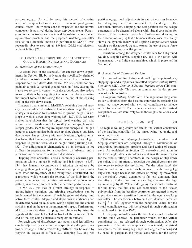
0 0.2 0.4 0.6 0.8 1−20

−18

−16

−14

−12

−10

−8

−6

−4

−2

0

2

time (s)

To

rso

An

gle

(deg

)

Fig. 4: Experimental data of the torso angle when stepping

down from the 2.5 inch platform.

Figure 4 shows the torso angle data. It can be seen that

the feedback system overreacts when correcting the forward-

pitching motion of the torso arising from the impact at step-

down. Moreover, this overreaction causes a second, very rapid,

forward-pitching motion of the torso. Because the angle of

the swing leg was controlled relative to the torso, the swing

leg rotated forward rapidly as well and impacted the ground

with sufficient force to break the leg. Though not reported

in [14], the experiment was repeated several times, with the

same result, namely, a broken leg following a 2.5 inch step-

down.

C. Active Force Control and Virtual Compliance for Shock

Absorption

To attenuate excessive torso pitching following a large step-

down, we adopted the idea of a switching controller from

[24], along with a active force control [25]. The height of

the platform, or equivalently, the depth of the step down, can

be immediately computed at impact from the lengths of the

robot’s legs and the angles of its joints. If the calculated height

of the platform is greater than 3 cm, the baseline controller

is replaced for one step with a controller whose purpose is to

attenuate pitching of the torso from the step-down disturbance.

Then, at the beginning of the very next step, the baseline

controller is re-applied.

The new controller, called a active force control, im-

poses virtual holonomic constraints on only three variables,

qLAsw, qmLSsw

, and qT, instead of four variables, as in the

baseline controller. In particular, the system input correspond-

ing to the stance motor leg shape is left free and is not used for

imposing a virtual constraint. Recall that this motor is in series

with a physical spring in the drivetrain, as shown in Figure 3.

Building on an idea developed in [26], [25] for bipedal running

on MABEL, we use the torque input of this motor to create an

additional virtual compliant element by defining the feedback,

umLSst(x) = −kvc (qmLSst

− qmLSvr)− kvd (qmLSst

) . (22)

For further use, we assemble the independent parameters of

the virtual compliance as αvc ∈ R3, defined as,

αvc = [kvc, kvd, qmLSvr]T . (23)

This feedback essentially turns the motor leg shape into

a shock absorber with stiffness kvc, damping kvd, and rest

position qmLSvr. As will be seen, this method of creating

a virtual compliant element serves to maintain good ground

contact forces (the friction cone is respected and the normal

component is positive) during large step-down events. Param-

eters in the controller were obtained by solving a constrained

optimization problem, and the proposed switching controller

resulted in a dramatic increase in performance: MABEL was

repeatedly able to step off an 8.0 inch (20.32 cm) platform

without falling [27].

IV. CONTROLLER DESIGN FOR LARGE UNEXPECTED

GROUND HEIGHT INCREASES AND DECREASES

A. Motivation of the Control Design

As established in the successful 20 cm step-down experi-

ments in Section III, by activating the specifically designed

step-down controller in the form of active force control, in

response to a step-down disturbance, MABEL could not only

maintain a positive vertical ground reaction force, causing the

stance toe to stay in contact with the ground, but also reduce

torso oscillation by a significant amount, thereby attenuating

the impact force on the swing toe at the end of the ensuing

step of the step-down event.

It appears that, similar to MABEL’s switching control strat-

egy for a step-down disturbance, humans also change their gait

strategy in response to disturbances in ground height, in up-

slope as well as down-slope walking [28], [29], [30]. Research

studies have shown that the typical level walking gait may

require small modifications for small grade ramps; however,

steeper grades seem to require significant changes in the gait

patterns to accommodate both large up-slope changes and large

down-slope changes. Along with modifications of gait patterns,

it is found that humans adjust the stiffness of the stance leg in

response to ground variations in height during running [31],

[32]. The adjustment is characterized by an increase in leg

stiffness in preparation for a step-down disturbance, and a

reduction in response to a step-up disturbance.

Tripping over obstacles is also a commonly occurring per-

turbation while a human is walking, and it is shown in [33],

[34] that humans accommodate a tripping disturbance by

changing their gait strategy. Cutaneous receptors are stimu-

lated when the trajectory of the swing foot is obstructed, and

a response which ensures the removal of the limb from the

perturbation, as well as the safe continuation of the locomotor

pattern, is activated to deal with the detected perturbation.

In MABEL, this idea of a reflex strategy in response to

ground-height variations and tripping perturbations can be

implemented in the context of switching-control design and

active force control. Step-up and step-down disturbances can

be detected based on calculated swing heights and the contact

switch signal on the toe at the moment of impact. Furthermore,

MABEL can also detect tripping over obstacles by using the

signals of the switch located in front of the shin and at the

end of toe, replacing cutaneous receptors in humans.

For each type of disturbance, gait pattern and leg stiffness

can be adjusted by switching to a specifically designed con-

troller. Changes in the effective leg stiffness can be made by

varying the values of stiffness kvc , damping kvd , and rest

position qmLSvr, and adjustments in gait pattern can be made

by redesigning the virtual constraints. In the design of the

controller, stiffness, damping, and rest position are the design

parameters to be determined along with virtual constraints for

the rest of the controlled variables. Furthermore, drawing on

the observation in [35] that a human’s stance knee essentially

shows the dynamic behavior of a spring-damper system when

walking on flat ground, we also extend the use of active force

control to walking over flat ground.

Transitions among the designed controllers for flat-ground

walking, stepping-down, stepping-up, and a trip-reflex will

be managed by a finite-state machine, which is presented in

Section V.

B. Summaries of Controller Designs

The controllers for flat-ground walking, stepping-down,

stepping-up, and a trip-reflex are called Regular-walking (RW),

Step-down (SD), Step-up (SU), and Tripping-reflex (TR) con-

trollers, respectively. This section summarizes the design pro-

cess of each controller.

1) Regular-Walking Controller: The regular-walking con-

troller is obtained from the baseline controller by replacing its

motor leg shape control with a virtual compliance to include

active force control. The parameter values for the virtual

compliance αvc are iteratively found thorough simulations, and

given by,

αvc = [1.8, 0.1297, 2.7]T. (24)

The regular-walking controller retains the virtual constraints

of the baseline controller for the torso, swing leg angle, and

swing leg shape.

2) Step-down and Step-up Controllers: Step-down and

Step-up controllers are designed through a combination of

constrained optimization problem and hand-tuning of param-

eters. As explained in Section III, excessive oscillation in

the torso angle after a step-down event was the main reason

for the robot’s falling. Therefore, in the design of step-down

controller, it is important to redesign the virtual constraint for

the torso to reduce the oscillation. On the other hand, the

baseline virtual constraints can be retained for the swing leg

angle and shape because the effects of swing leg movement

on the robot’s overall dynamics is far less dominant than

the effects of the torso and stance leg (because the legs

are relatively light). When redesigning the virtual constraint

for the torso, the first and last coefficients of the Bezier

polynomials from the baseline controller are retained in order

to provide a smooth transition from and to the regular-walking

controller. The coefficients between them, denoted hereafter

by α2···5T ∈ R

4, together with the parameter values for the

virtual compliance αvc will be selected through optimization

as explained in Section IV-C.

The step-up controller uses the baseline virtual constraint

for the torso whereas the parameter values for the virtual

compliance αvc are selected through optimization. After the

parameters of the virtual compliance are obtained, the virtual

constraints for the swing leg shape and angle are redesigned

by hand. In particular, the virtual constraints for the swing

(a) (b) (c)

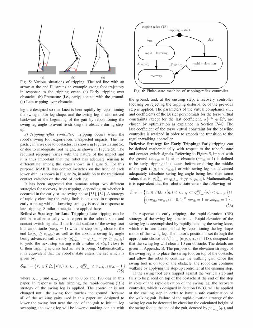
Fig. 5: Various situations of tripping. The red line with an

arrow at the end illustrates an example swing foot trajectory

in response to the tripping event. (a) Early tripping over

obstacles. (b) Premature (i.e., early) contact with the ground.

(c) Late tripping over obstacles.

leg are designed so that knee is bent rapidly by repositioning

the swing motor leg shape, and the swing leg is also moved

backward at the beginning of the gait by repositioning the

swing leg angle to avoid re-striking the obstacle during step-

up.

3) Tripping-reflex controller: Tripping occurs when the

robot’s swing foot experiences unexpected impacts. The im-

pacts can arise due to obstacles, as shown in Figures 5a and 5c,

or due to inadequate foot height, as shown in Figure 5b. The

required response varies with the nature of the impact and

it is thus important that the robot has adequate sensing to

differentiate among the cases shown in Figure 5. For this

purpose, MABEL has contact switches on the front of each

lower shin, as shown in Figure 2a, in addition to the traditional

contact switches on the end of each leg.

It has been suggested that humans adopt two different

strategies for recovery from tripping, depending on whether it

occurred in the early or late swing phase [33], [34]. A strategy

of rapidly elevating the swing limb is activated in response to

early tripping while a lowering strategy is used in response to

late tripping. Similar strategies are applied here.

Reflexive Strategy for Late Tripping: Late tripping can be

defined mathematically with respect to the robot’s state and

contact switch signals. If the frontal surface of the swing foot

hits an obstacle (swsh = 1) with the step being close to the

end (s(qs) ≥ searly) as well as the absolute swing leg angle

being advanced sufficiently (qabsLAsw:= qLAsw

+ qT ≥ qearly)

to yield the next step starting with a value of s(qs) close to

0, then tripping is classified as late tripping. Mathematically,

it is equivalent that the robot’s state enters the set which is

given by,

SRL :={

xs ∈ TQs

∣

∣s(qs) ≥ searly, qabsLAsw

≥ qearly, swsh = 1}

,(25)

where searly and qearly are set to 0.66 and 190 deg in this

paper. In response to late tripping, the rapid-lowering (RL)

strategy of the swing leg is applied. The controller is not

changed until the swing foot touches the ground. Because

all of the walking gaits used in this paper are designed to

lower the swing foot near the end of the gait to initiate leg

swapping, the swing leg will be lowered making contact with

tripping-reflex (TR)

rapid− lowering

recovery

rapid− elevation

tripping − start

SRL SRE

S(RE,RC)S(RL,RC)

Fig. 6: Finite-state machine of tripping-reflex controller

the ground, and, at the ensuing step, a recovery controller

focusing on rejecting the tripping disturbance of the previous

step is applied. The parameters of the virtual compliance αvc,

and coefficients of the Bezier polynomials for the torso virtual

constraints except for the last coefficient, α1···5T ∈ R

5, are

chosen by optimization as explained in Section IV-C. The

last coefficient of the torso virtual constraint for the baseline

controller is retained in order to smooth the transition to the

regular-walking controller.

Reflexive Strategy for Early Tripping: Early tripping can

be defined mathematically with respect to the robot’s state

and contact switch signals. Referring to Figure 5, impact with

the ground (swtoe = 1) or an obstacle (swsh = 1) is defined

to be early tripping if it occurs before or during the middle

of the gait (s(qs) < searly) or with swing leg not advanced

adequately (absolute swing leg angle being less than some

value, that is, qabsLAsw:= qLAsw

+ qT < qearly). Mathematically,

it is equivalent that the robot’s state enters the following set

SRE :={

xs ∈ TQs

∣

∣s(qs) < searly or qabsLAsw(qs) < qearly

}

∩{

(swsh, swtoe) ∈ {0, 1}2|swsh = 1 or swtoe = 1

}

.

(26)

In response to early tripping, the rapid-elevation (RE)

strategy of the swing leg is activated. Rapid-elevation of the

swing leg is accomplished by rapidly bending the swing knee,

which is in turn accomplished by repositioning the leg shape

motor of the swing leg. The motor’s position is set through the

appropriate choice of hd,vmLSsw

(θ(qs), αv) in (18), designed so

that the swing leg will clear a 10 cm obstacle. The details are

given in Appendix B. The purpose of the elevation strategy of

the swing leg is to place the swing foot on top of the obstacle,

and allow the robot to continue the walking gait. Once the

swing foot is on top of the obstacle, the robot can continue

walking by applying the step-up controller at the ensuing step.

If the swing foot gets trapped against the vertical step and

fails to be placed on top of the obstacle at the end of the step

in spite of the rapid-elevation of the swing leg, the recovery

controller, which is designed in Section IV-B3, will be applied

at the ensuing step in order to have a safe continuation of

the walking gait. Failure of the rapid-elevation strategy of the

swing leg can be detected by checking the calculated height of

the swing foot at the end of the gait, denoted by pvtoesw(qs), and

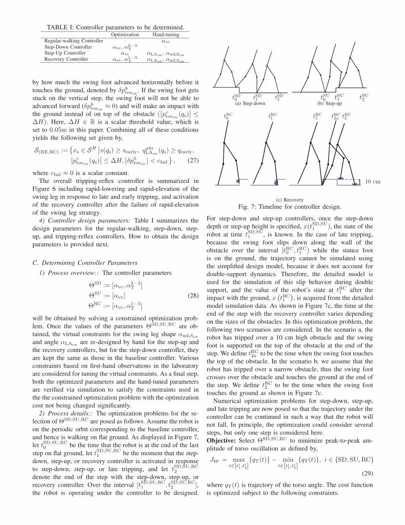
TABLE I: Controller parameters to be determined.Optimization Hand-tuning

Regular-walking Controller · αvc

Step-Down Controller αvc, α2···5

T·

Step-Up Controller αvc αLAsw, αmLSsw

Recovery Controller αvc, α1···5

TαLAsw

, αmLSsw

by how much the swing foot advanced horizontally before it

touches the ground, denoted by δphtoesw . If the swing foot gets

stuck on the vertical step, the swing foot will not be able to

advanced forward (δphtoesw ≈ 0) and will make an impact with

the ground instead of on top of the obstacle (∣

∣pvtoesw(qs)∣

∣ ≤∆H). Here, ∆H ∈ R is a scalar threshold value, which is

set to 0.05m in this paper. Combining all of these conditions

yields the following set given by,

S(RE,RC) :={

xs ∈ SH∣

∣s(qs) ≥ searly, qabsLAsw(qs) ≥ qearly,

∣

∣pvtoesw(qs)∣

∣ ≤ ∆H,∣

∣δphtoesw∣

∣ < cfail}

, (27)

where cfail ≈ 0 is a scalar constant.

The overall tripping-reflex controller is summarized in

Figure 6 including rapid-lowering and rapid-elevation of the

swing leg in response to late and early tripping, and activation

of the recovery controller after the failure of rapid-elevation

of the swing leg strategy.

4) Controller design parameters: Table I summarizes the

design parameters for the regular-walking, step-down, step-

up, and tripping-reflex controllers. How to obtain the design

parameters is provided next.

C. Determining Controller Parameters

1) Process overview:: The controller parameters

ΘSD := [αvc, α2···5T ]

ΘSU := [αvc] (28)

ΘRC := [αvc, α1···5T ]

will be obtained by solving a constrained optimization prob-

lem. Once the values of the parameters ΘSD,SU,RC are ob-

tained, the virtual constraints for the swing leg shape αmLSsw

and angle αLAsware re-designed by hand for the step-up and

the recovery controllers, but for the step-down controller, they

are kept the same as those in the baseline controller. Various

constraints based on first-hand observations in the laboratory

are considered for tuning the virtual constraints. As a final step,

both the optimized parameters and the hand-tuned parameters

are verified via simulation to satisfy the constraints used in

the the constrained optimization problem with the optimization

cost not being changed significantly.

2) Process details:: The optimization problems for the se-

lection of ΘSD,SU,RC are posed as follows. Assume the robot is

on the periodic orbit corresponding to the baseline controller,

and hence is walking on flat ground. As displayed in Figure 7,

let tSD,SU,RC0 be the time that the robot is at the end of the last

step on flat ground, let tSD,SU,RC1 be the moment that the step-

down, step-up, or recovery controller is activated in response

to step-down, step-up, or late tripping, and let tSD,SU,RC2

denote the end of the step with the step-down, step-up, or

recovery controller. Over the interval [tSD,SU,RC1 , tSD,SU,RC

2 ],the robot is operating under the controller to be designed.

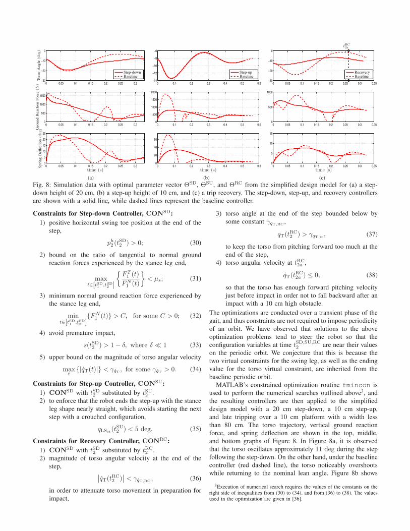
tSD0 tSD1 tSD2(a) Step-down

tSU0 tSU1 tSU2(b) Step-up

tRC0 tRC

1tRC1 tRC

2a tRC2

10 cm

(c) Recovery

Fig. 7: Timeline for controller design.

For step-down and step-up controllers, once the step-down

depth or step-up height is specified, x(tSD,SU1 ), the state of the

robot at time tSD,SU1 , is known. In the case of late tripping,

because the swing foot slips down along the wall of the

obstacle over the interval [tRC0 , tRC

1 ) while the stance foot

is on the ground, the trajectory cannot be simulated using

the simplified design model, because it does not account for

double-support dynamics. Therefore, the detailed model is

used for the simulation of this slip behavior during double

support, and the value of the robot’s state at tRC1 after the

impact with the ground, x(

tRC1

)

, is acquired from the detailed

model simulation data. As shown in Figure 7c, the time at the

end of the step with the recovery controller varies depending

on the sizes of the obstacles. In this optimization problem, the

following two scenarios are considered. In the scenario a, the

robot has tripped over a 10 cm high obstacle and the swing

foot is supported on the top of the obstacle at the end of the

step. We define tRC2a to be the time when the swing foot touches

the top of the obstacle. In the scenario b, we assume that the

robot has tripped over a narrow obstacle, thus the swing foot

crosses over the obstacle and touches the ground at the end of

the step. We define tRC2 to be the time when the swing foot

touches the ground as shown in Figure 7c.

Numerical optimization problems for step-down, step-up,

and late tripping are now posed so that the trajectory under the

controller can be continued in such a way that the robot will

not fall. In principle, the optimization could consider several

steps, but only one step is considered here.

Objective: Select ΘSD,SU,RC to minimize peak-to-peak am-

plitude of torso oscillation as defined by,

JΘi = maxt∈[ti1,ti2]

{qT(t)} − mint∈[ti1,ti2]

{qT(t)}, i ∈ {SD, SU,RC}

(29)

where qT(t) is trajectory of the torso angle. The cost function

is optimized subject to the following constraints.

0 0.05 0.1 0.15 0.2 0.25 0.3−30

−20

−10

0

0 0.05 0.1 0.15 0.2 0.25 0.30

500

1000

1500

0 0.05 0.1 0.15 0.2 0.25 0.30

5

10

15

20

25

time (s)

Tors

oA

ngle

(deg)

Gro

und

Rea

ctio

nF

orc

e(N

)S

pri

ng

Defl

ecti

on(deg)

Step-downBaseline

(a)

0 0.1 0.2 0.3 0.4 0.5 0.6−14

−12

−10

−8

−6

0 0.1 0.2 0.3 0.4 0.5 0.60

500

1000

1500

2000

0 0.1 0.2 0.3 0.4 0.5 0.60

20

40

60

time (s)

Step-upBaseline

(b)

0 0.05 0.1 0.15 0.2 0.25 0.3 0.35−30

−20

−10

0

0 0.05 0.1 0.15 0.2 0.25 0.3 0.350

500

1000

0 0.05 0.1 0.15 0.2 0.25 0.3 0.350

5

10

15

time (s)

tRC

2a

RecoveryBaseline

(c)

Fig. 8: Simulation data with optimal parameter vector ΘSD, ΘSU, and ΘRC from the simplified design model for (a) a step-

down height of 20 cm, (b) a step-up height of 10 cm, and (c) a trip recovery. The step-down, step-up, and recovery controllers

are shown with a solid line, while dashed lines represent the baseline controller.

Constraints for Step-down Controller, CONSD:

1) positive horizontal swing toe position at the end of the

step,

ph2 (tSD2 ) > 0; (30)

2) bound on the ratio of tangential to normal ground

reaction forces experienced by the stance leg end,

maxt∈[tSD1 ,tSD2 ]

{

FT1 (t)

FN1 (t)

}

< µs; (31)

3) minimum normal ground reaction force experienced by

the stance leg end,

mint∈[tSD1 ,tSD2 ]

{FN1 (t)} > C, for some C > 0; (32)

4) avoid premature impact,

s(tSD2 ) > 1− δ, where δ ≪ 1 (33)

5) upper bound on the magnitude of torso angular velocity

maxt

{|qT(t)|} < γqT , for some γqT > 0. (34)

Constraints for Step-up Controller, CONSU:

1) CONSD with tSD2 substituted by tSU2 .

2) to enforce that the robot ends the step-up with the stance

leg shape nearly straight, which avoids starting the next

step with a crouched configuration,

qLSst(tSU2 ) < 5 deg. (35)

Constraints for Recovery Controller, CONRC:

1) CONSD with tSD2 substituted by tRC

2 .

2) magnitude of torso angular velocity at the end of the

step,∣

∣qT(tRC2 )

∣

∣ < γqT,RC, (36)

in order to attenuate torso movement in preparation for

impact,

3) torso angle at the end of the step bounded below by

some constant γqT,RC,

qT(tRC2 ) > γqT,rc

, (37)

to keep the torso from pitching forward too much at the

end of the step,

4) torso angular velocity at tRC2a ,

qT(tRC2a ) ≤ 0, (38)

so that the torso has enough forward pitching velocity

just before impact in order not to fall backward after an

impact with a 10 cm high obstacle.

The optimizations are conducted over a transient phase of the

gait, and thus constraints are not required to impose periodicity

of an orbit. We have observed that solutions to the above

optimization problems tend to steer the robot so that the

configuration variables at time tSD,SU,RC2 are near their values

on the periodic orbit. We conjecture that this is because the

two virtual constraints for the swing leg, as well as the ending

value for the torso virtual constraint, are inherited from the

baseline periodic orbit.

MATLAB’s constrained optimization routine fmincon is

used to perform the numerical searches outlined above3, and

the resulting controllers are then applied to the simplified

design model with a 20 cm step-down, a 10 cm step-up,

and late tripping over a 10 cm platform with a width less

than 80 cm. The torso trajectory, vertical ground reaction

force, and spring deflection are shown in the top, middle,

and bottom graphs of Figure 8. In Figure 8a, it is observed

that the torso oscillates approximately 11 deg during the step

following the step-down. On the other hand, under the baseline

controller (red dashed line), the torso noticeably overshoots

while returning to the nominal lean angle. Figure 8b shows

3Execution of numerical search requires the values of the constants on theright side of inequalities from (30) to (34), and from (36) to (38). The valuesused in the optimization are given in [36].

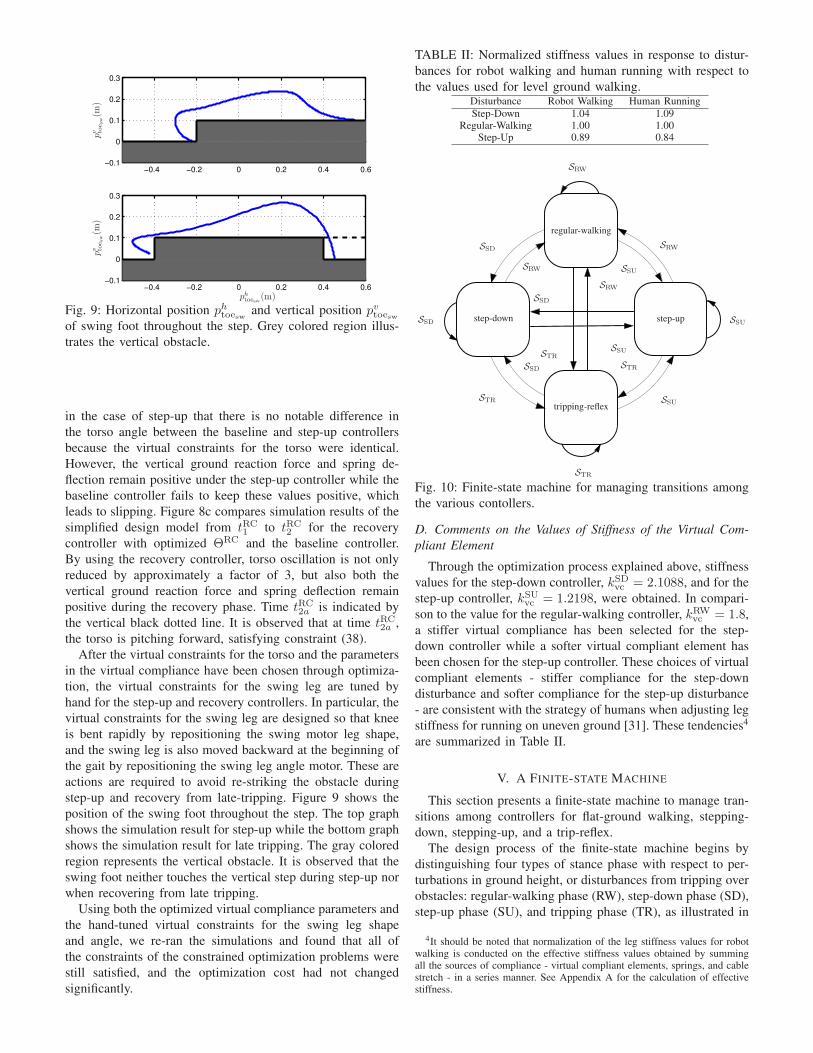
−0.4 −0.2 0 0.2 0.4 0.6−0.1

0

0.1

0.2

0.3

−0.4 −0.2 0 0.2 0.4 0.6−0.1

0

0.1

0.2

0.3

phtoesw

(m)

pv toesw(m

)pv toesw(m

)

Fig. 9: Horizontal position phtoesw and vertical position pvtoeswof swing foot throughout the step. Grey colored region illus-

trates the vertical obstacle.

in the case of step-up that there is no notable difference in

the torso angle between the baseline and step-up controllers

because the virtual constraints for the torso were identical.

However, the vertical ground reaction force and spring de-

flection remain positive under the step-up controller while the

baseline controller fails to keep these values positive, which

leads to slipping. Figure 8c compares simulation results of the

simplified design model from tRC1 to tRC

2 for the recovery

controller with optimized ΘRC and the baseline controller.

By using the recovery controller, torso oscillation is not only

reduced by approximately a factor of 3, but also both the

vertical ground reaction force and spring deflection remain

positive during the recovery phase. Time tRC2a is indicated by

the vertical black dotted line. It is observed that at time tRC2a ,

the torso is pitching forward, satisfying constraint (38).

After the virtual constraints for the torso and the parameters

in the virtual compliance have been chosen through optimiza-

tion, the virtual constraints for the swing leg are tuned by

hand for the step-up and recovery controllers. In particular, the

virtual constraints for the swing leg are designed so that knee

is bent rapidly by repositioning the swing motor leg shape,

and the swing leg is also moved backward at the beginning of

the gait by repositioning the swing leg angle motor. These are

actions are required to avoid re-striking the obstacle during

step-up and recovery from late-tripping. Figure 9 shows the

position of the swing foot throughout the step. The top graph

shows the simulation result for step-up while the bottom graph

shows the simulation result for late tripping. The gray colored

region represents the vertical obstacle. It is observed that the

swing foot neither touches the vertical step during step-up nor

when recovering from late tripping.

Using both the optimized virtual compliance parameters and

the hand-tuned virtual constraints for the swing leg shape

and angle, we re-ran the simulations and found that all of

the constraints of the constrained optimization problems were

still satisfied, and the optimization cost had not changed

significantly.

TABLE II: Normalized stiffness values in response to distur-

bances for robot walking and human running with respect to

the values used for level ground walking.Disturbance Robot Walking Human Running

Step-Down 1.04 1.09Regular-Walking 1.00 1.00

Step-Up 0.89 0.84

regular-walking

step-down step-up

tripping-reflex

SRW

SRW

SRW

SRW

SSU

SSU

SSU

SSU

STR

STR

STR

STR

SSD

SSD

SSD

SSD

Fig. 10: Finite-state machine for managing transitions among

the various contollers.

D. Comments on the Values of Stiffness of the Virtual Com-

pliant Element

Through the optimization process explained above, stiffness

values for the step-down controller, kSDvc = 2.1088, and for the

step-up controller, kSUvc = 1.2198, were obtained. In compari-

son to the value for the regular-walking controller, kRWvc = 1.8,

a stiffer virtual compliance has been selected for the step-

down controller while a softer virtual compliant element has

been chosen for the step-up controller. These choices of virtual

compliant elements - stiffer compliance for the step-down

disturbance and softer compliance for the step-up disturbance

- are consistent with the strategy of humans when adjusting leg

stiffness for running on uneven ground [31]. These tendencies4

are summarized in Table II.

V. A FINITE-STATE MACHINE

This section presents a finite-state machine to manage tran-

sitions among controllers for flat-ground walking, stepping-

down, stepping-up, and a trip-reflex.

The design process of the finite-state machine begins by

distinguishing four types of stance phase with respect to per-

turbations in ground height, or disturbances from tripping over

obstacles: regular-walking phase (RW), step-down phase (SD),

step-up phase (SU), and tripping phase (TR), as illustrated in

4It should be noted that normalization of the leg stiffness values for robotwalking is conducted on the effective stiffness values obtained by summingall the sources of compliance - virtual compliant elements, springs, and cablestretch - in a series manner. See Appendix A for the calculation of effectivestiffness.

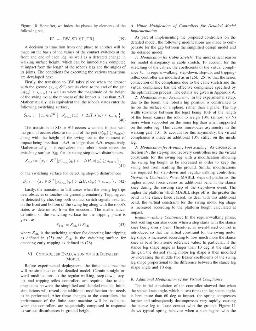
Figure 10. Hereafter, we index the phases by elements of the

following set,

W := {RW, SD, SU,TR} . (39)

A decision to transition from one phase to another will be

made on the basis of the values of the contact switches at the

front and end of each leg, as well as a detected change in

walking surface height, which can be immediately computed

at impact from the length of the robot’s legs and the angles of

its joints. The conditions for executing the various transitions

are developed next.

Firstly, the transition to RW takes place when the impact

with the ground (xs ∈ SH ) occurs close to the end of the gait

(s(qs) ≥ searly) as well as when the magnitude of the height

of the swing toe at the moment of the impact is less than ∆H .

Mathematically, it is equivalent that the robot’s states enter the

following switching surface,

SRW :={

xs ∈ SH∣

∣

∣

∣pvtoesw(qs)∣

∣ ≤ ∆H, s(qs) ≥ searly}

.(40)

The transition to SD or SU occurs when the impact with

the ground occurs close to the end of the gait (s(qs) ≥ searly),

along with the height of the swing toe at the moment of

impact being less than −∆H , or larger than ∆H , respectively.

Mathematically, it is equivalent that robot’s state enters the

switching surface SSD for detecting step-down disturbances

SSD :={

xs ∈ SH∣

∣pvtoesw(qs) < −∆H, s(qs) ≥ searly}

,(41)

or the switching surface for detecting step-up disturbances

SSU :={

xs ∈ SH∣

∣pvtoesw(qs) > ∆H, s(qs) ≥ searly}

. (42)

Lastly, the transition to TR arises when the swing leg trips

over obstacles or touches the ground prematurely. Tripping can

be detected by checking both contact switch signals installed

on the front and bottom of the swing leg along with the robot’s

states as determined from the encoders. The mathematical

definition of the switching surface for the tripping phase is

given as

STR := SRL ∪ SRE, (43)

where SRL is the switching surface for detecting late tripping

as defined in (25) and SRE is the switching surface for

detecting early tripping as defined in (26).

VI. CONTROLLER EVALUATION ON THE DETAILED

MODEL

Before experimental deployment, the finite-state machine

will be simulated on the detailed model. Certain straightfor-

ward modifications to the regular-walking, step-down, step-

up, and tripping-reflex controllers are required due to dis-

crepancies between the simplified and detailed models. Initial

simulations will reveal one additional modification that needs

to be performed. After these changes to the controllers, the

performance of the finite-state machine will be evaluated

when the controllers are sequentially composed in response

to various disturbances in ground height.

A. Minor Modification of Controllers for Detailed Model

Implementation

As part of implementing the proposed controllers on the

detailed model, the following modifications are made to com-

pensate for the gap between the simplified design model and

the detailed model.

1) Modification for Cable Stretch: The most critical reason

for model discrepancy is cable stretch. To account for the

stretching of the cables, the coefficients of the virtual compli-

ance kvc in regular-walking, step-down, step-up, and tripping-

reflex controller are modified as in [26], [25] so that the series

connection of the compliance due to the cable stretch and the

virtual compliance has the effective compliance specified by

the optimization process. The details are given in Appendix A.

2) Modification for Asymmetry: In the experimental setup,

due to the boom, the robot’s hip position is constrained to

lie on the surface of a sphere, rather than a plane. The hip

width (distance between the legs) being 10% of the length

of the boom causes the robot to weigh 10% (almost 70 N)

more when supported on the inner leg than when supported

on the outer leg. This causes inner-outer asymmetry in the

walking gait [13]. To account for this asymmetry, the virtual

compliance is made an additional 10% stiffer on the inside

leg.

3) Modification for Avoiding Foot Scuffing: As discussed in

Section IV, the step-up and recovery controllers use the virtual

constraints for the swing leg with a modification allowing

the swing leg height to be increased in order to keep the

swing foot from scuffing the ground. Similar modifications

are required for step-down and regular-walking controllers.

Step-down Controller: When MABEL steps off platforms, the

higher impact force causes an additional bend in the stance

knee during the ensuing step of the step-down event. The

higher the platform which MABEL steps off is, the greater the

bend in the stance knee caused. To deal with this additional

bend, the virtual constraint for the swing motor leg shape

is increased according to the platform height calculated at

impact.

Regular-walking Controller: In the regular-walking phase,

foot scuffing can also occur when a step starts with the stance

knee being overly bent. Therefore, an event-based control is

introduced so that the virtual constraint for the swing motor

leg shape is increased according to how much more the stance

knee is bent from some reference value. In particular, if the

stance leg shape angle is larger than 10 deg at the start of

the gait, the desired swing motor leg shape is then modified

by increasing the middle two Bezier coefficients of the swing

leg shape proportional to the difference between the stance leg

shape angle and 10 deg.

B. Additional Modification of the Virtual Compliance

The initial simulation of the controller showed that when

the stance knee angle, which is two times the leg shape angle,

is bent more than 60 deg at impact, the spring compresses

further and subsequently decompresses very rapidly, causing

the stance leg to loose contact with the ground. Figure 11

shows typical spring behavior when a step begins with the

0 0.1 0.2 0.3 0.4 0.5 0.6−10

0

10

20

30

time (s)

Spri

ng

Defl

ecti

on(deg)

W/O modificationWith Modification

Fig. 11: Simulation data of a step with the stance knee being

excessively bent at the start. The dashed line shows simulation

result without modification on the virtual compliance, and the

solid line illustrates simulation result with modification. The

small circles on the plot indicate the end of the step.

RW → RE → RW → RE → RW

(a) Small Ramp

RW → RL → RC → SU → RW

(b) Stair

RW → RE → RW → RE → RW

(c) Small Bump

RW → SD → RW

(d) Step-down

RW → RE → SU → RE → RC → SU → SU → RW

(e) Two Consecutive Stairs

RW → RE → SU → RE → RC → SU → RW → SD → RE → RW

(f) Step-up and Step-down of Two Consecutive Stairs

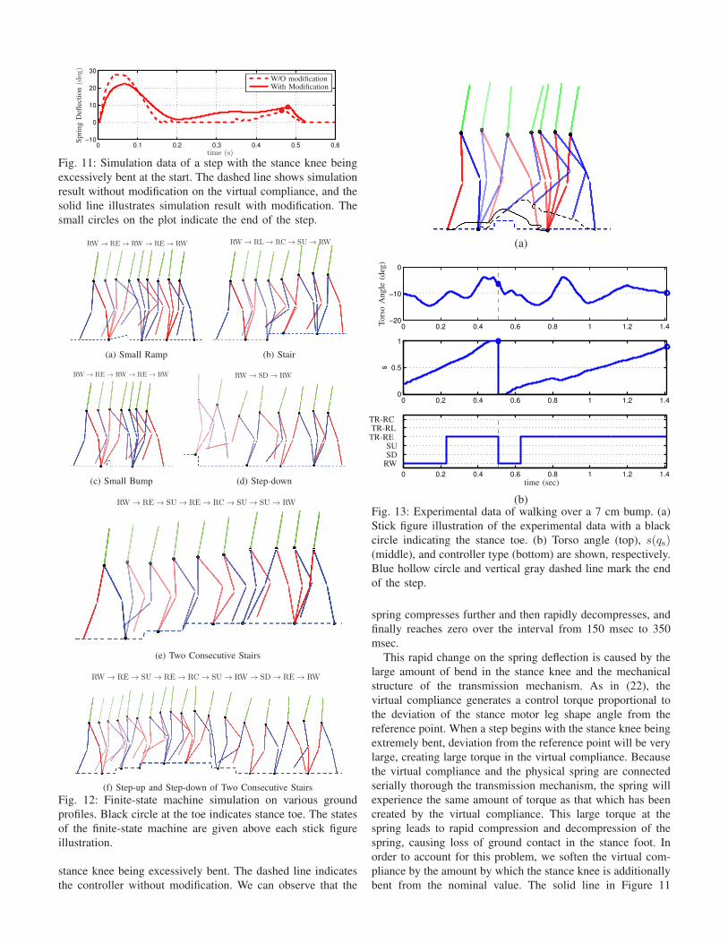
Fig. 12: Finite-state machine simulation on various ground

profiles. Black circle at the toe indicates stance toe. The states

of the finite-state machine are given above each stick figure

illustration.

stance knee being excessively bent. The dashed line indicates

the controller without modification. We can observe that the

(a)

0 0.2 0.4 0.6 0.8 1 1.2 1.4−20

−10

0

0 0.2 0.4 0.6 0.8 1 1.2 1.40

0.5

1

s

0 0.2 0.4 0.6 0.8 1 1.2 1.4

time (sec)

Tors

oA

ngle

(deg

)

TR-RCTR-RL

TR-RESUSD

RW

(b)Fig. 13: Experimental data of walking over a 7 cm bump. (a)

Stick figure illustration of the experimental data with a black

circle indicating the stance toe. (b) Torso angle (top), s(qs)(middle), and controller type (bottom) are shown, respectively.

Blue hollow circle and vertical gray dashed line mark the end

of the step.

spring compresses further and then rapidly decompresses, and

finally reaches zero over the interval from 150 msec to 350

msec.

This rapid change on the spring deflection is caused by the

large amount of bend in the stance knee and the mechanical

structure of the transmission mechanism. As in (22), the

virtual compliance generates a control torque proportional to

the deviation of the stance motor leg shape angle from the

reference point. When a step begins with the stance knee being

extremely bent, deviation from the reference point will be very

large, creating large torque in the virtual compliance. Because

the virtual compliance and the physical spring are connected

serially thorough the transmission mechanism, the spring will

experience the same amount of torque as that which has been

created by the virtual compliance. This large torque at the

spring leads to rapid compression and decompression of the

spring, causing loss of ground contact in the stance foot. In

order to account for this problem, we soften the virtual com-

pliance by the amount by which the stance knee is additionally

bent from the nominal value. The solid line in Figure 11

0 0.5 1 1.5 2 2.5 3 3.5−20

−10

0

0 0.5 1 1.5 2 2.5 3 3.50

20

40

0 0.5 1 1.5 2 2.5 3 3.5

time (sec)

Tors

oA

ngle

(deg

)S

pri

ng

Defl

ecti

on

(N)

TR-RCTR-RL

TR-RESUSD

RW

0 0.5 1 1.5 2 2.5 3 3.5−20

−10

0

0 0.5 1 1.5 2 2.5 3 3.50

20

40

0 0.5 1 1.5 2 2.5 3 3.5

time (sec)

Tors

oA

ngle

(deg

)S

pri

ng

Defl

ecti

on

(N)

TR-RCTR-RL

TR-RESUSD

RW

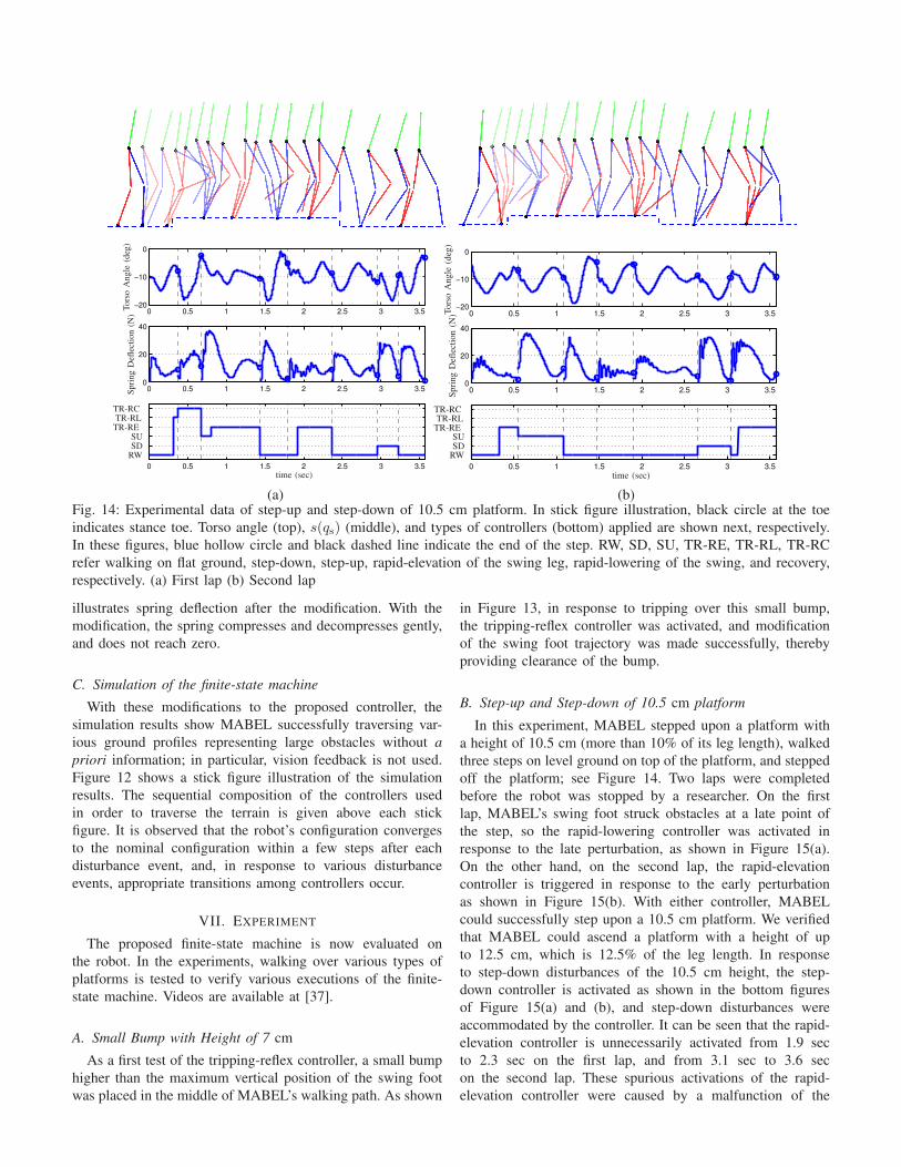
(a) (b)Fig. 14: Experimental data of step-up and step-down of 10.5 cm platform. In stick figure illustration, black circle at the toe

indicates stance toe. Torso angle (top), s(qs) (middle), and types of controllers (bottom) applied are shown next, respectively.

In these figures, blue hollow circle and black dashed line indicate the end of the step. RW, SD, SU, TR-RE, TR-RL, TR-RC

refer walking on flat ground, step-down, step-up, rapid-elevation of the swing leg, rapid-lowering of the swing, and recovery,

respectively. (a) First lap (b) Second lap

illustrates spring deflection after the modification. With the

modification, the spring compresses and decompresses gently,

and does not reach zero.

C. Simulation of the finite-state machine

With these modifications to the proposed controller, the

simulation results show MABEL successfully traversing var-

ious ground profiles representing large obstacles without a

priori information; in particular, vision feedback is not used.

Figure 12 shows a stick figure illustration of the simulation

results. The sequential composition of the controllers used

in order to traverse the terrain is given above each stick

figure. It is observed that the robot’s configuration converges

to the nominal configuration within a few steps after each

disturbance event, and, in response to various disturbance

events, appropriate transitions among controllers occur.

VII. EXPERIMENT

The proposed finite-state machine is now evaluated on

the robot. In the experiments, walking over various types of

platforms is tested to verify various executions of the finite-

state machine. Videos are available at [37].

A. Small Bump with Height of 7 cm

As a first test of the tripping-reflex controller, a small bump

higher than the maximum vertical position of the swing foot

was placed in the middle of MABEL’s walking path. As shown

in Figure 13, in response to tripping over this small bump,

the tripping-reflex controller was activated, and modification

of the swing foot trajectory was made successfully, thereby

providing clearance of the bump.

B. Step-up and Step-down of 10.5 cm platform

In this experiment, MABEL stepped upon a platform with

a height of 10.5 cm (more than 10% of its leg length), walked

three steps on level ground on top of the platform, and stepped

off the platform; see Figure 14. Two laps were completed

before the robot was stopped by a researcher. On the first

lap, MABEL’s swing foot struck obstacles at a late point of

the step, so the rapid-lowering controller was activated in

response to the late perturbation, as shown in Figure 15(a).

On the other hand, on the second lap, the rapid-elevation

controller is triggered in response to the early perturbation

as shown in Figure 15(b). With either controller, MABEL

could successfully step upon a 10.5 cm platform. We verified

that MABEL could ascend a platform with a height of up

to 12.5 cm, which is 12.5% of the leg length. In response

to step-down disturbances of the 10.5 cm height, the step-

down controller is activated as shown in the bottom figures

of Figure 15(a) and (b), and step-down disturbances were

accommodated by the controller. It can be seen that the rapid-

elevation controller is unnecessarily activated from 1.9 sec

to 2.3 sec on the first lap, and from 3.1 sec to 3.6 sec

on the second lap. These spurious activations of the rapid-

elevation controller were caused by a malfunction of the

(a)

(b)Fig. 15: Stick figure illustration of experimental data of step-

up and step-down of 10.5 cm platform. Black circle at the toe

indicates stance toe. (a) On the first lap, the rapid-lowering

controller is activated in response to late tripping while in (b),

on the second lap, the rapid-elevation controller is triggered

in response to early tripping.

contact switches5.

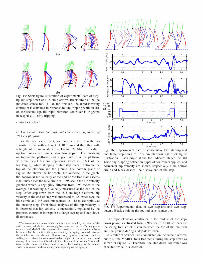
C. Consecutive Two Step-ups and One Large Step-down of

18.5 cm platform

For the next experiment, we built a platform with two

stair-steps, one with a height of 10.5 cm and the other with

a height of 8 cm as shown in Figure 16. MABEL walked

up two consecutive risers, took two steps of level walking

on top of the platform, and stepped off from the platform

with one step (18.5 cm step-down, which is 18.5% of the

leg length), while skipping a stair-step placed between the

top of the platform and the ground. The bottom graph of

Figure 16b shows the horizontal hip velocity. In the graph,

the horizontal hip velocity at the end of the two stair ascents

is 0.9 m/sec (see the blue circle at 1.295 sec in the hip velocity

graphs.) which is negligibly different from 0.93 m/sec of the

average flat-walking hip velocity measured at the end of the

step. After step-down from the 18.5 cm high platform, hip

velocity at the end of step was increased to 1.8 m/sec (see the

blue circle at 3.148 sec), but reduced to 1.12 m/sec rapidly at

the ensuing step. From these analyses of the hip velocity, it

is observed that hip velocity is successfully regulated by the

proposed controller in response to large step-up and step-down

disturbances.

5The erroneous activation of the switches was caused by vibration of theswitch covers, which have non-negligible mass and inertia. During gentlemaneuvers of MABEL, the vibration of the switch covers was not a problembecause it had been efficiently damped out by the spring installed betweenthe switch covers and the shin. However, very dynamic maneuvers such aswalking over obstacles with considerable height did cause an unexpectedclosing of the contact switches due to the vibration of the switch. This smallissue on the contact switches could be solved by a redesign of the contactswitch mechanism, such as adding more damping on the springs.

0 0.5 1 1.5 2 2.5 3 3.5

−20

−10

0

0 0.5 1 1.5 2 2.5 3 3.50

20

40

0 0.5 1 1.5 2 2.5 3 3.5

0 0.5 1 1.5 2 2.5 3 3.50

1

2

time (sec)

time (sec)

Tors

oA

ngle

(deg

)S

pri

ng

Defl

ecti

on

(N)

TR-RCTR-RL

TR-RESUSD

RW

Hip

Vel

oci

ty(m

/sec

)

Fig. 16: Experimental data of consecutive two step-up and

one large step-down of 18.5 cm platform. (a) Stick figure

illustration. Black circle at the toe indicates stance toe. (b)

Torso angle, spring deflection, types of controllers applied, and

horizontal hip velocity are shown, respectively. Blue hollow

circle and black dashed line display end of the step.

Fig. 17: Experimental data of two step-ups and two step-

downs. Black circle at the toe indicates stance toe.

The rapid-elevation controller in the middle of the step-

down phase is activated from 2.919 sec to 3.148 sec because

the swing foot struck a stair between the top of the platform

and the ground during a step-down event.

A similar experiment was conducted on the same platform,

but this time MABEL took two steps during the step-down as

shown in Figure 17. Therefore, the step-down controller was

executed twice in succession.

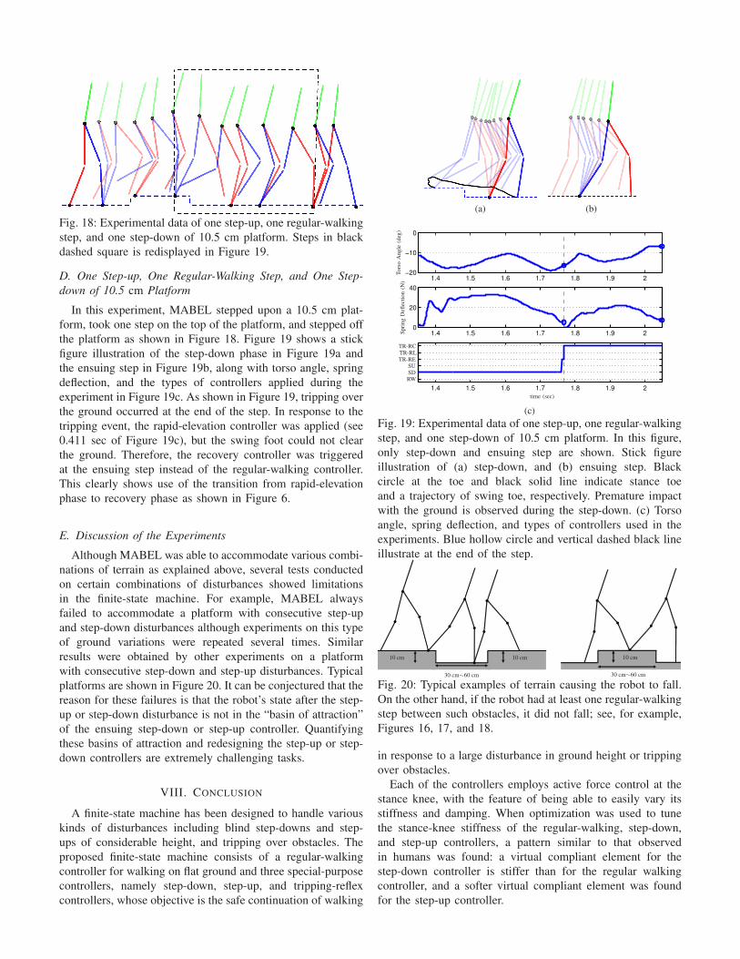
Fig. 18: Experimental data of one step-up, one regular-walking

step, and one step-down of 10.5 cm platform. Steps in black

dashed square is redisplayed in Figure 19.

D. One Step-up, One Regular-Walking Step, and One Step-

down of 10.5 cm Platform

In this experiment, MABEL stepped upon a 10.5 cm plat-

form, took one step on the top of the platform, and stepped off

the platform as shown in Figure 18. Figure 19 shows a stick

figure illustration of the step-down phase in Figure 19a and

the ensuing step in Figure 19b, along with torso angle, spring

deflection, and the types of controllers applied during the

experiment in Figure 19c. As shown in Figure 19, tripping over

the ground occurred at the end of the step. In response to the

tripping event, the rapid-elevation controller was applied (see

0.411 sec of Figure 19c), but the swing foot could not clear

the ground. Therefore, the recovery controller was triggered

at the ensuing step instead of the regular-walking controller.

This clearly shows use of the transition from rapid-elevation

phase to recovery phase as shown in Figure 6.

E. Discussion of the Experiments

Although MABEL was able to accommodate various combi-

nations of terrain as explained above, several tests conducted

on certain combinations of disturbances showed limitations

in the finite-state machine. For example, MABEL always

failed to accommodate a platform with consecutive step-up

and step-down disturbances although experiments on this type

of ground variations were repeated several times. Similar

results were obtained by other experiments on a platform

with consecutive step-down and step-up disturbances. Typical

platforms are shown in Figure 20. It can be conjectured that the

reason for these failures is that the robot’s state after the step-

up or step-down disturbance is not in the “basin of attraction”

of the ensuing step-down or step-up controller. Quantifying

these basins of attraction and redesigning the step-up or step-

down controllers are extremely challenging tasks.

VIII. CONCLUSION

A finite-state machine has been designed to handle various

kinds of disturbances including blind step-downs and step-

ups of considerable height, and tripping over obstacles. The

proposed finite-state machine consists of a regular-walking

controller for walking on flat ground and three special-purpose

controllers, namely step-down, step-up, and tripping-reflex

controllers, whose objective is the safe continuation of walking

(a) (b)

1.4 1.5 1.6 1.7 1.8 1.9 2−20

−10

0

1.4 1.5 1.6 1.7 1.8 1.9 20

20

40

1.4 1.5 1.6 1.7 1.8 1.9 2

time (sec)T

ors

oA

ngle

(deg

)S

pri

ng

Defl

ecti

on

(N)

TR-RCTR-RLTR-RE

SUSDRW

(c)

Fig. 19: Experimental data of one step-up, one regular-walking

step, and one step-down of 10.5 cm platform. In this figure,

only step-down and ensuing step are shown. Stick figure

illustration of (a) step-down, and (b) ensuing step. Black

circle at the toe and black solid line indicate stance toe

and a trajectory of swing toe, respectively. Premature impact

with the ground is observed during the step-down. (c) Torso

angle, spring deflection, and types of controllers used in the

experiments. Blue hollow circle and vertical dashed black line

illustrate at the end of the step.

10 cm10 cm10 cm

30 cm∼60 cm30 cm∼60 cm

Fig. 20: Typical examples of terrain causing the robot to fall.

On the other hand, if the robot had at least one regular-walking

step between such obstacles, it did not fall; see, for example,

Figures 16, 17, and 18.

in response to a large disturbance in ground height or tripping

over obstacles.

Each of the controllers employs active force control at the

stance knee, with the feature of being able to easily vary its

stiffness and damping. When optimization was used to tune

the stance-knee stiffness of the regular-walking, step-down,

and step-up controllers, a pattern similar to that observed

in humans was found: a virtual compliant element for the

step-down controller is stiffer than for the regular walking

controller, and a softer virtual compliant element was found

for the step-up controller.

The tripping-reflex controller is designed to behave in

different manners with respect to early or late tripping: a rapid

elevating strategy of the swing leg is activated in response

to early tripping while a rapid lowering strategy is used

in response to late tripping. This rapid lowering strategy is

followed by a recovery phase which is designed to reject the

previous step’s disturbance.

Experimentation with this controller showed MABEL

traversing various kinds of obstacles including 12.5 cm blind

step-ups, and 18.5 cm blind step-downs, as well as various

combinations of step-ups and step-downs, such as short stacks

of stairs.

Although the proposed finite-state machine shows good

performance on various terrain profiles, the video in [38]

shows limited controller performance to attenuate the influ-

ence of random variations in ground height on the robot’s

speed. To improve controller performance in the face of such

disturbances, it would be interesting to explore an outer-loop

discrete-event-based control design which can be layered onto

the present controller.

REFERENCES

[1] K. Byl and R. Tedrake, “Metastable walking machines,” International

Journal of Robotics Research, vol. 28, pp. 1040–1064, August 2009.[2] R. T. Katie Byl, “Metastable walking on stochastically rough terrain,” in

Proceedings of Robotics: Science and Systems IV, Zurich, Switzerland,June 2008.

[3] K. Byl and R. Tedrake, “Approximate optimal control of the compassgait on rough terrain,” in IEEE International Conference on Robotics

and Automation, may 2008, pp. 1258 –1263.[4] D. Hobbelen and M. Wisse, “A disturbance rejection measure for

limit cycle walkers: The gait sensitivity norm,” IEEE Transactions on

Robotics, vol. 23, no. 6, pp. 1213 –1224, dec. 2007.[5] ——, “Swing-leg retraction for limit cycle walkers improves disturbance

rejection,” IEEE Transactions on Robotics, vol. 24, no. 2, pp. 377 –389,april 2008.

[6] M. Wisse, A. L. Schwab, R. Q. van der Linde, and F. C. T. van derHelm, “How to keep from falling forward: Elementary swing leg actionfor passive dynamic walkers,” IEEE Transactions on Robotics, vol. 21,no. 3, pp. 393–401, June 2005.

[7] I. R. Manchester, U. Mettin, F. Iida, and R. Tedrake, “Stable dynamicwalking over uneven terrain,” The International Journal of Robotics

Research, 2011.[8] I. R. Manchester, “Transverse dynamics and regions of stability for

nonlinear hybrid limit cycles.” in Proceedings of the 18th IFAC World

Congress, 2011.[9] C. Sabourin, O. Bruneau, and G. Buche, “Control strategy for the robust

dynamic walk of a biped robot,” The International Journal of Robotics

Research, vol. 25, no. 9, pp. 843–860, Sept. 2006.[10] Q. Huang and Y. Nakamura, “Sensory reflex control for humanoid

walking,” IEEE Transactions on Robotics, vol. 21, no. 5, pp. 977 –984, oct. 2005.

[11] G. N. Boone and J. K. Hodgins, “Slipping and tripping reflexes forbipedal robots,” Autonomous Robots, vol. 4, pp. 259–271, July 1997.

[12] J. Grizzle, J. Hurst, B. Morris, H.-W. Park, and K. Sreenath, “MABEL,a new robotic bipedal walker and runner,” in American Control Confer-

ence, St. Louis, MO, USA, June 2009, pp. 2030–2036.[13] K. Sreenath, H.-W. Park, I. Poulakakis, and J. W. Grizzle, “A compliant

hybrid zero dynamics controller for stable, efficient and fast bipedalwalking on MABEL,” The International Journal of Robotics Research,vol. 30, no. 9, pp. 1170–1193, Aug 2011.

[14] H.-W. Park, K. Sreenath, J. Hurst, and J. Grizzle, “Identification ofa bipedal robot with a compliant drivetrain,” IEEE Control Systems

Magazine, vol. 31, no. 2, pp. 63 –88, april 2011.[15] J. W. Hurst, “The role and implementation of compliance in legged

locomotion,” Ph.D. dissertation, Robotics Institute, Carnegie MellonUniversity, Pittsburgh, PA, August 2008.

[16] R. Alexander, “Three uses for springs in legged locomotion,” The

International Journal of Robotics Research, vol. 9, no. 2, pp. 53–61,1990.

[17] W. Khalil and E. Dombre, Modeling, Identification and Control of

Robots. Bristol, PA, USA: Taylor & Francis, Inc., 2002.[18] Y. Hurmuzlu and D. B. Marghitu, “Rigid Body Collisions of Planar

Kinematic Chains With Multiple Contact Points,” The International

Journal of Robotics Research, vol. 13, no. 1, pp. 82–92, 1994.[19] C. Canudas de Wit, H. Olsson, K. Astrom, and P. Lischinsky, “A new

model for control of systems with friction,” IEEE Transactions on

Automatic Control, vol. 40, no. 3, pp. 419–425, Mar. 1995.[20] F. Plestan, J. Grizzle, E. Westervelt, and G. Abba, “Stable walking of a

7-DOF biped robot,” IEEE Transactions on Robotics and Automation,vol. 19, no. 4, pp. 653–668, Aug. 2003.

[21] E. R. Westervelt, J. W. Grizzle, C. Chevallereau, J. H. Choi, andB. Morris, Feedback Control of Dynamic Bipedal Robot Locomotion.Taylor & Francis/CRC Press, 2007.

[22] C. C. de Wit, “On the concept of virtual constraints as a tool for walkingrobot control and balancing,” Annual Reviews in Control, vol. 28, no. 2,pp. 157–166, 2004.

[23] H.-W. Park. (2010) First attempt at walking over rough groundfor bipedal robot mabel. Youtube Video. [Online]. Available:http://youtu.be/IlWIWf4daNs

[24] T. Yang, E. Westervelt, and A. Serrani, “A framework for the controlof stable aperiodic walking in underactuated planar bipeds,” in IEEE

International Conference on Robotics and Automation, Roma, Italy,April 2007, pp. 4661–4666.

[25] K. Sreenath, H.-W. Park, , and J. W. Grizzle, “Embedding active forcecontrol within the compliant hybrid zero dynamics to achieve stable,fast running on mabel,” The International Journal of Robotics Research,2012, submitted.

[26] K. Sreenath, “Feedback control of a bipedal walker and runner withcompliance,” Ph.D. dissertation, The University of Michigan, 2011.

[27] H.-W. Park, K. Sreenath, A. Ramezani, and J. Grizzle, “Switchingcontrol design for accommodating large step-down disturbances inbipedal robot walking.” in IEEE International Conference on Robotics

and Automation, 2012, to appear.[28] S. D. Prentice, E. N. Hasler, J. J. Groves, and J. S. Frank, “Locomotor

adaptations for changes in the slope of the walking surface,” Gait &

Posture, vol. 20, no. 3, pp. 255 – 265, 2004.[29] K. Kawamura, A. Tokuhiro, and H. Takechi, “Gait analysis of slope

walking: a study on step length, stride width, time factors and deviationin the center of pressure,” Acta Med Okayama, vol. 45, no. 3, pp. 179– 184, 1991.

[30] A. Tokuhiro, H. Nagashima, and H. Takechi, “Electromyographic kine-siology of lower extremity muscles during slope walking,” Arch Phys

Med Rehabil, vol. 66, no. 9, pp. 610 – 613, 1985.[31] S. Grimmer, M. Ernst, M. Gunther, and R. Blickhan, “Running on

uneven ground: leg adjustment to vertical steps and self-stability,”Journal of Experimental Biology, vol. 211, no. 18, pp. 2989–3000, 2008.

[32] R. Muller and R. Blickhan, “Running on uneven ground: Leg adjust-ments to altered ground level,” Human Movement Science, vol. 29, no. 4,pp. 578 – 589, 2010.

[33] J. J. Eng, D. A. Winter, and A. E. Patla, “Strategies for recovery from atrip in early and late swing during human walking,” Experimental Brain

Research, vol. 102, pp. 339–349, 1994.[34] ——, “Intralimb dynamics simplify reactive control strategies during

locomotion,” Journal of Biomechanics, vol. 30, no. 6, pp. 581 – 588,1997.

[35] R. W. Sinnet, M. J. Powell, R. P. Shah, and A. D. Ames, “A human-inspired hybrid control approach to bipedal robotic walking,” in 18th

IFAC World Congress, 2011.[36] H.-W. Park, “Control of a bipedal robot walker on rough terrain,” Ph.D.

dissertation, The University of Michigan, 2012.[37] ——. (2012) Bipedal robot mabel traverses uneven terrain using

touch instead of sight. Youtube Video. [Online]. Available: http://youtu.be/MhPSZOUgZ 8

[38] ——. (2011) Bipedal robot mabel walks over randomly varyingground: Experiment no. 1. Youtube Video. [Online]. Available:http://youtu.be/m8-j7s6-bzE

APPENDIX A

MODIFICATION ON VIRTUAL COMPLIANCE AND

CALCULATION OF EFFECTIVE STIFFNESS

MABEL has three sources of compliance: physical springs

installed on the torso, virtual compliance created by the leg

shape motor, and compliance due to the cable stretch. Because

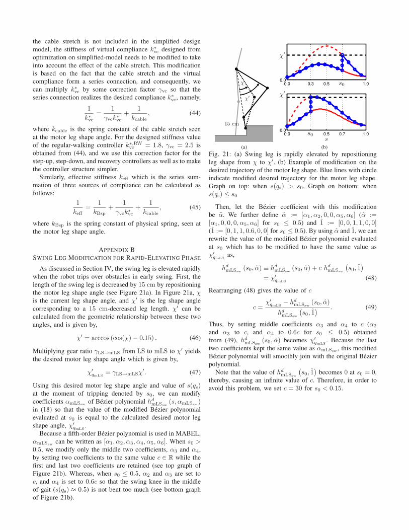
the cable stretch is not included in the simplified design

model, the stiffness of virtual compliance k∗vc designed from

optimization on simplified-model needs to be modified to take

into account the effect of the cable stretch. This modification

is based on the fact that the cable stretch and the virtual

compliance form a series connection, and consequently, we

can multiply k∗vc by some correction factor γvc so that the

series connection realizes the desired compliance k∗vc, namely,

1

k∗vc=

1

γvck∗vc+

1

kcable, (44)

where kcable is the spring constant of the cable stretch seen

at the motor leg shape angle. For the designed stiffness value

of the regular-walking controller k∗,RWvc = 1.8, γvc = 2.5 is

obtained from (44), and we use this correction factor for the

step-up, step-down, and recovery controllers as well as to make

the controller structure simpler.

Similarly, effective stiffness keff which is the series sum-

mation of three sources of compliance can be calculated as

follows:

1

keff=

1

kBsp+

1

γvck∗vc+

1

kcable, (45)

where kBsp is the spring constant of physical spring, seen at

the motor leg shape angle.

APPENDIX B

SWING LEG MODIFICATION FOR RAPID-ELEVATING PHASE

As discussed in Section IV, the swing leg is elevated rapidly

when the robot trips over obstacles in early swing. First, the

length of the swing leg is decreased by 15 cm by repositioning

the motor leg shape angle (see Figure 21a). In Figure 21a, χis the current leg shape angle, and χ′ is the leg shape angle

corresponding to a 15 cm-decreased leg length. χ′ can be

calculated from the geometric relationship between these two

angles, and is given by,

χ′ = arccos (cos(χ)− 0.15) . (46)

Multiplying gear ratio γLS→mLS from LS to mLS to χ′ yields

the desired motor leg shape angle which is given by,

χ′

qmLS= γLS→mLSχ

′. (47)

Using this desired motor leg shape angle and value of s(qs)at the moment of tripping denoted by s0, we can modify

coefficients αmLSswof Bezier polynomial hd

mLSsw(s, αmLSsw

)in (18) so that the value of the modified Bezier polynomial

evaluated at s0 is equal to the calculated desired motor leg

shape angle, χ′

qmLS.

Because a fifth-order Bezier polynomial is used in MABEL,

αmLSswcan be written as [α1, α2, α3, α4, α5, α6]. When s0 >

0.5, we modify only the middle two coefficients, α3 and α4,

by setting two coefficients to the same value c ∈ R while the

first and last two coefficients are retained (see top graph of

Figure 21b). Whereas, when s0 ≤ 0.5, α2 and α3 are set to

c, and α4 is set to 0.6c so that the swing knee in the middle

of gait (s(qs) ≈ 0.5) is not bent too much (see bottom graph

of Figure 21b).

15 cm

χ

χ′

(a)

0.0 0.3 0.5 1.00.0

0.0 0.5 0.7 1.00.0

s0

s0

χ′

χ′

s(b)

Fig. 21: (a) Swing leg is rapidly elevated by repositioning

leg shape from χ to χ′. (b) Example of modification on the

desired trajectory of the motor leg shape. Blue lines with circle

indicate modified desired trajectory for the motor leg shape.

Graph on top: when s(qs) > s0, Graph on bottom: when

s(qs) ≤ s0

Then, let the Bezier coefficient with this modification

be α. We further define α := [α1, α2, 0, 0, α5, α6] (α :=[α1, 0, 0, 0, α5, α6] for s0 ≤ 0.5) and 1 := [0, 0, 1, 1, 0, 0](1 := [0, 1, 1, 0.6, 0, 0] for s0 ≤ 0.5). By using α and 1, we can

rewrite the value of the modified Bezier polynomial evaluated

at s0 which has to be modified to have the same value as

χ′

qmLSas,

hdmLSsw

(s0, α) ≡ hdmLSsw

(s0, α) + c hdmLSsw

(

s0, 1)

= χ′

qmLS(48)

Rearranging (48) gives the value of c

c =χ′

qmLS− hd

mLSsw(s0, α)

hdmLSsw

(

s0, 1) . (49)

Thus, by setting middle coefficients α3 and α4 to c (α2

and α3 to c, and α4 to 0.6c for s0 ≤ 0.5) obtained

from (49), hdmLSsw

(s0, α) becomes χ′

qmLS. Because the last

two coefficients kept the same value as αmLSsw, this modified

Bezier polynomial will smoothly join with the original Bezier

polynomial.

Note that the value of hdmLSsw

(

s0, 1)

becomes 0 at s0 = 0,

thereby, causing an infinite value of c. Therefore, in order to

avoid this problem, we set c = 30 for s0 < 0.15.