ELSEVIER Journal of Computational and Apphed Mathematics 90 (1998) 95-116

JOURNAL OF COMPUTATIONAL AND APPLIED MATHEMATICS

A finite difference method for the Korteweg-de Vries and the Kadomtsev-Petviashvili equations

Bao-Feng Feng a, Taketomo Mitsui b,, a Department oJ Aeronautics and Astronautws, Kyoto Unwerstty, Kyoto 606-01, Japan b Graduate School of Human Informatws, Nagoya Unwersuy, Nagoya 464-01, Japan

Recewed 29 March 1997; recewed tn revised form 9 January 1998; accepted 9 January 1998

Abstract

A hnearized imphcit fimte difference method for the Korteweg-de Vries equation is proposed and straightforwardly extended to the Kadomtsev-Petviashvili equation. We investigate the order of accuracy of the method and prove the method to be unconditionally hnearly stable. The numerical experiments for the Korteweg~te Vnes and the Kadomtsev- Petvlashvfll equations are car'ned out wtth various conditions. Numerical results for the collision of two lump type solitary wave solutions to the Kadomtsev-Petviashvlh equation are also reported. (~) ! 998 Elsevier Science B V. All rights reserved.

Keywords Korteweg~de Vnes, Kadomtsev-Petvlashvlh; Llne-soliton; Lump type soliton; Lmearized implicit finite &fference method

1. Introduction

About a hundred years ago, Korteweg and de Vries [18] derived an equation equivalent to

Ut +(3U2)x +Urxr=O ( t > 0 , - o o < x < o c ) (1.1)

to describe approximately the slow evolution o f long water waves o f moderate amplitude as they propagate under the influence o f gravity in one direction in shallow o f uniform depth. In 1965, Zabusky and Kruskal discovered the concept o f the solitons while studying the results o f a numerical computation on the Kor teweg-de Vries (KdV) equation (1.1). Since then, there has been considerable interest in solitons and the related soliton equations. Analytical solutions are available for certain nonlinear evolution equations via the Inverse Scattering Transformation (IST) developed by Garder et al. [8]. However, for some other nonlinear equations, no analytical solutions are known and numerical studies are essential in order to develop an understanding o f the phenomena.

* Corresponding author. E-mall: a41794a@nucc.ec.nagoya-u.ac jp.

0377-0427/98/$19.00 @ 1998 Elsevier Science B.V. All rights reserved PH S0377-0427(98)00006-5

96 B - F Fen#, T. Mttsul/Journal oJ Computattonal and Apphed Mathematws 90 (1998) 95 116

Y axts

X ax is

Fig 1. Lump solution of the KPI equation.

The two-dimensional KdV, or Kadomtsev-Petviashvili (KP) equation

Utx q- (3U2)xx + Uxr~x -- 30.2Uyy = 0 ( t > 0 , - - C ~ < x , y < c ~ ) (1.2)

was first introduced by Kadomtsev and Petviashvili [15] in order to study the stability of one- dimensional solitons against transverse perturbations. In the case of o -2= 1, Eq. (1.2) is usually called the KPI equation, whereas in the case of 0 .2 = - 1, the KPII equation. The KP equation is the two-dimensional generalization of the KdV equation. It is shown that the choice of the sign of o .2 is critical with respect to the stability characteristics of line-solitons. For the KPI equation, there exits a lump type soliton solution which decay as O(1/r:), r 2 =x2+ y2 when r---~ oo. This lump solution can be expressed as

4 { - [ x + 2y + 3(22 - ]12)t] 2 q-/t2(y q- 62Q 2 + 1 /# 2 } u(x,y,,)= (1.3)

which is shown in Fig. 1 It is worth noting that the lump solution takes both positive and negative values and the total

mass of this solitary wave, defined by

f_~ /_~ u(x,y,t)dxdy (1.4)

is identically zero. The KP equation, a soliton equation important from analytical and numerical point of view, is

one of the few known completely integrable equations in the multi-dimensional soliton equations. Thus in the last few years, considerable interest has been focused on the KP equation.

On the basis of the great success in the soliton theory, much efforts have been done to investi- gations of soliton properties in multi-dimensional systems. Exact solutions describing interactions of quasi-one-dimensional solitons were obtained for systems with two or three spatial dimensions as a straightforward extension of the one-dimensional soliton. Spatially localized solitary wave solutions decaying in all directions are also obtained analytically for some multi-dimensional soliton equa- tions such as the KP equation. But the numerical solution of the multi-dimensional soliton equations

B - F . Fen(], T Mt t suH Journal o f Computa twna l and Apphed Mathemat tcs 90 (1998) 95-116 97

cannot be', obtained straightforwardly from that of one-dimensional case and often raises a difficult problem. Although several numerical schemes have been proposed for the KdV equation (see [5, 11. 12, 22, 26, 27, 29]), the numerical analysis literature for the KP equation is extremely small. As far as we are aware of, only two kinds of method are reported. These include: the explicit finite difference method proposed by Katsis [16]; the pseudo-spectral method developed by Fornberg and "~hitham (see [20, 28]).

"['he purpose of this paper is to develop a finite difference method for multi-dimensional soliton equations. We propose a linearized implicit method for the KdV equation and extend it to the KP equation successfully.

!n Secuon 2 we propose a linearized implicit method for the KdV equation and extend it to the KP equation. Section 3 is devoted to the analysis of these methods with respect to the accuracy, the stability and the numerical dispersion. After considerations on the numerical boundary conditions in Section 4, numerical experiments with various initial conditions for the KdV and KP equations are reported in Section 5. A good agreement is obtained while comparing the analytical and the numerical solutions. We investigate the interaction of two localized solitary waves, which is still unknown analytically. In Section 6, we give a brief summary and further aspects in our future study.

2. Linearized implicit methods for the KdV and KP equations

First we introduce some usual finite difference operators and give some of their properties, which wall be cseful in constructing and analyzing our finite difference schemes. Suppose we wish to solve a partial differential equation with the dependent variable u ( x , y , t ) . For convenience, let us assume that the spacing of the grid points in the x-direction is uniform, and given by Ax, while the spacing of tl',,~ poinls in the y-direction, also uniform, by A y . We approximate the grid value u ( lAx , m A y , n A t )

by u n We define the central-difference operators as I,m"

H~uT, m " " (2.1) Ul+ l , m - - U l _ l . m ,

6~Ul~.m = U" -- U" (2.2) 1+½,m I--½.rn'

" n z U n n (~vUl.m Lm+½ - - Ul, m- -½' (2.3)

(~2 un n n n l,m (~x(fxUl.m) = -- 2Ul, m q- n (2.4) = UI+I, m Ul- - l .m~

'~ n (~-vU l. m " " n n n n O v ( b v U l , m ) = - - 2Ut. m q- (2.5) ~- Ul .m+ I Ul .m- - l "

Furthermore, we introduce higher differences as

-4 , 2 2 , , , " " " (2.6) OrUl , m = (~r( ( ~ x U l . m ) = UI+2, m - - 4U1+1, m -'k 6ut, m - 4 U l _ l . m --k U l _ 2 , m ,

-2 , _ , , " " (2.7) Hxr~Ul, m - - Ul+2, m -- 2Ul+l, m + 2Ut_t ,m - - U l _ 2 , m.

98 B.-F Fen q. T Mitsui / Journal oJ Computattonal and Apphed Mathemattcs 90 (1998) 95-116

Thus partial derivatives are approximated through the finite difference operators as

O~X I.m nruT"m ~2U ¢~2ulnm = 2Ax + O(Ax2 )" ~x 2 I.m - - ( -~x)2 "~- O ( A x 2 )'

~2U l,m 2 n l,m 2 n _ _ (~ v U l m O3U _ _ - - Hx6xUl, m q_ O ( A x 2 ) ,

Oy 2 ( A y ) 2 + O(Ay2), ~ x 3 2(Ax)------T

¢~4 u (~4Ulnra ,.,. - + O( Ax2 )"

2.1. Linearized implicit methods f o r the K d V equation

(2.8)

o r

utx + fxx + Ux~x = O, (2.9)

where f = 3u 2. Through the Crank-Nicolson scheme as well as the central-difference formulas (2.1)- (2.7), we have

mx z n+l 4 n /,/7+1) = tu, - uT) + p f Z ( f ; + f ; + ' ) + r6~(u, + O, (2.10)

w h e r e p : A t / A x , r = A t / ( A x ) 3, u T ~ u ( l A x , n A t ) , l : l , 2 . . . . . L . T o f i n d u n+l = i.ull" n+ l , "2"n+l , . . . , U~+I]T

from u", a set of nonlinear algebraic equations has to be solved. To overcome this difficulty, a way linearizing the implicit scheme (2.10) is presented. The linearized form is obtained by using Taylor's expansion of f7 +t about the nth time-level. Thus we apply

i.+, : i . + (0j )" \ 0 t / t \ 0 t 2 ) + "

f f + l : f 7 n n+l + D t A u l + O(AtZ), (2.11)

where D7 : ( O f / O u ) 7 : 6 u ~ ' and Au7 +1 : u ~ '+n - u 7. From (2.11), the nonlinear part in (2.10) can be approximated as

: r )nA. n+l f~+~ + f7 (3u7) 2 + (3u7 +' )2 : 2f~ + ...., ~u, + O(At 2)

-- 6uT+'u7 + O(At2). (2.12)

Substituting (2.12) into (2.10) yields the following penta-diagonal system.

n n+l hn n+l n n+l n n+l n n+l n atul_ 2 -}- t,.lUl_ 1 ~- etu t + cluz+ 1 + atut+ 2 : d I. (2.13)

Here the coefficients are calculated from u" through

a 7 = r , b 7 = 6 p u 7 _ , - 4 r - l , c 7=6pu7+ , - 4 r + l , e 7 = 6 r - 1 2 p u 7

Keeping a direct extension to the KP equation in mind, we discretlze the alternative form of the KdV equation proposed by Djidjeli et al. [4]:

B.-F Feng, T Mttsut/ Journal of Computattonal and Apphed Mathemattcs 90 (1998) 95 116 99

and

d 7 = uT+ , - uT_ ~ - r(uT+ 2 - 4u7+ , + 6u 7 - 4u7_ , + uT_:).

The vector form of Eq. (2.13) can be expressed as

A . u n+l = d n, ( 2 . 1 4 )

with

H n + l ~

]" u n + I 1

u n + l

¢ n + l L - - I

. n + l . hi' L

A __

a l l a12 a13

a21 a22 ". ' .

a31

0 • •

0

aLL

and d" [ d ~ , d ~ . . . . , T = , dL] . We have to compute the coefficient matrix A and solve the penta-diagonal system of equations (2.14) at each time step.

2.2. L i n e a r i z e d impl ic t t m e t h o d s f o r the K P equat ion

Let us consider how to extend the previously proposed scheme of KdV equation to the conservative form of the KPI equation

ut~ + f ~ + uxx.,~ - 3uvv = 0, ( 2 . 1 5 )

where f denotes 3 u 2 in this case, too. An introduction of the second order finite difference for the term uH, implies a finite difference

method to the KP equation given by

H . n + l n 2 n f n + l ~ 4 n . n + l "2 n . n + l rtUl, m -- Ul, m) q- p~v( f ] ,m + al, m l " ~ r(~r(Ul .m-~ Ul. m ) - - 3 q O v ( u / , m + Ul. m ) = 0 . (2.16)

where p = A t / A x , q = A t A x / ( A y ) 2, r = A t / ( A x ) 3, u/, m" . . . . ~ u ( l A x , m A y , nA t ) , l = 1 , 2 , ,L , m =

1 , 2 , . . . , M .

Similar to the KdV case, the linearized form of (2.16) is obtained through Taylor's expansion. . n + l _ _ . n + l That is, with the notations D " =(Of/OU)Tm :6UT, m and Aul , m - - u / , m I.m , --UT.m, the equation

f ln+l n I-~ n A n + l ,m = f / , m ~-Z'~l, mZJUl, m +O(At2)

admits the calculation

f /n+l n n ,m q- f l , m = 2f;,m -- "-'" " "+' + Z~t.m/lU/. m + O ( A t 2) __ .- .+ l , - - o u l , m u/, m + O(At2). (2.17)

Substitution of (2.17) into (2.16) and some manipulations derive the following linear system of equations:

n n + l t n n + l n n + l n n + l - - n n + l ~ n n + l - - n n + l n a/ mUl.m_l ~- OLmUI_2, m ~- Cl, mUl_l , m --~ gl, mUl, m -+- el, mUl+l,m q- Oi.mUl+2. m -]- a/,mUl,m+ ] : d l , m. (2.18)

1 O0 B -F Feng, T Mitsut / Journal oJ Computat tonal and Appl ied Mathemat tcs 90 (1998) 95-116

The coefficients are given by

11 = - 3q, blnm = r, al.m

glnm : 6r - 12pul~,m + 6q,

and

C11 11 I,m = 6puz--I, , , -- 4 r -- 1,

eT. m = 6puT+l. m -- 4 r + 1,

11 11 11 11 11 I1 I1 dl . m = Ul+l. m - Ul_l . m - r(l.l/+2, m -- 4Ul+l. m -~- 6ULm -- 4Ul_ l . m -~- UT_e.m)

_~_ 11 11 11 3q(Ul,m+ j -- 2Uz, m + Ul, m_l ).

The vector form of (2.18) is

A • u 11+1 = d11,

-u,(+J •

u n + 1 LI

. n + l U n+l = t"/12 ~ .,4 =

. n + l

. lgLM .

with

a l l a12 a13

a21 a22 " ' .

"• , • , • a31

" , , " , .

" , • am I

0 •

a i m

" . • • • •

• • • • • .

• • , " • .

• . • • • •

-

"•° :~

" ,• ~<

(2.19)

11 11 d11 iv The coefficient matrix A is a nonsymmetric band one and a very and d11 = [d~'l,...,dLi,dl2 . . . . , LMJ •

limited number of its elements will be changed depending on the boundary conditions we adopt in the actual computation.

3. Analyses of the methods

3.1. O r d e r o f a c c u r a c y

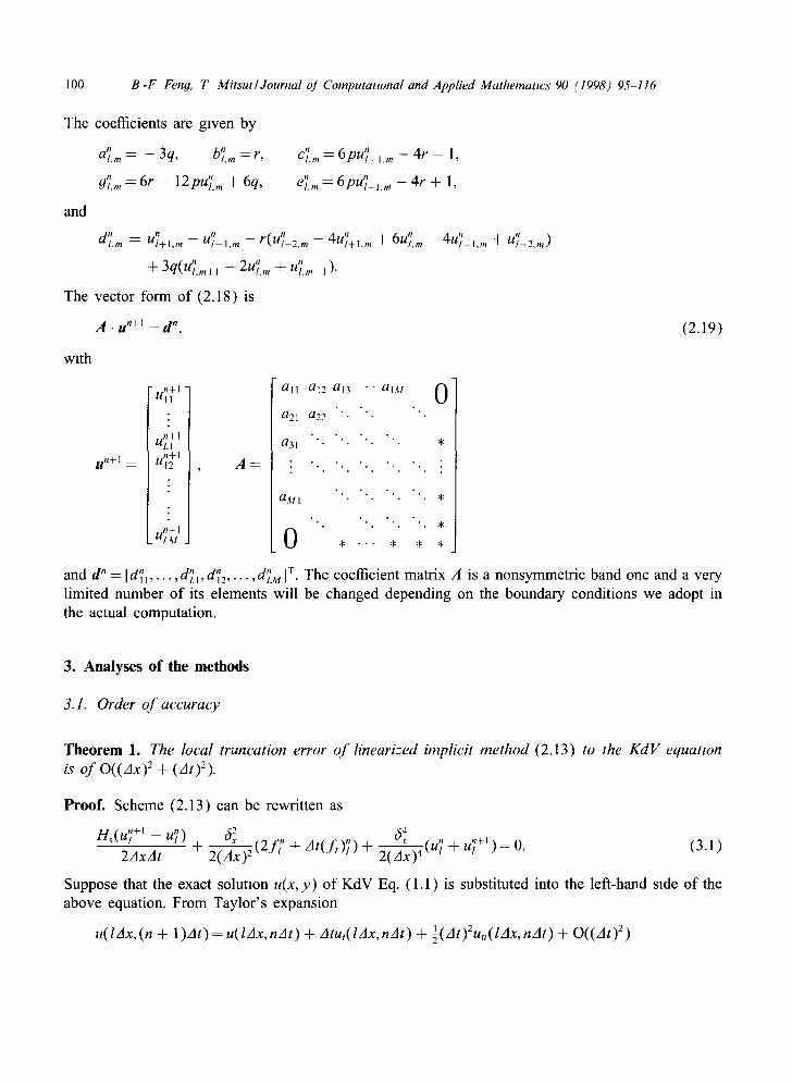
Theorem 1. The local truncation error o f l i n e a r i z e d impl ic i t m e t h o d (2.13) to the K d V e q u a t i o n

is o f O((Ax) 2 + (At):).

Proof. Scheme (2.13) can be rewritten as

n ~ ( u 7 +1 - uT) c~ ¢2 ,e n ~4 tu" u7 +1 ~ - x A t t + ~ ' J ' + A t ( f t ) 7 ) + 2(~-~x)4, , + )=0. (3.1)

Suppose that the exact solution u(x, y ) of KdV Eq. (1.1) is substituted into the left-hand side of the above equation• From Taylor's expansion

u( lAx,(n + 1)At)--u(lAx, nAt) + Atut(lAx, nAt) + l (At)Zu,( lAx, nAt) + O((At) z)

B-F Fen(l, T Mttsut/Journal oj Computattonal and Apphed Mathematws 90 (1998) 95-116 101

and Eq. (2.8), we can derive

(ut(lAx, nAt) 4- f~(lAx, nAt) 4- ux~(lAx, nAt))~ 4- ½At(ut(lAx, nAt) 4- f~(lAx, nAt)

4-u~(lAx, nAt))t~ + O((Ax) 2 + (At) 2) = 0. (3.2)

Because u(lAx, nat) is the exact solution of KdV Eq. (1.1), we obviously have

ut(lAx, nat) + f~(lAx, nat) + Ux~x(IAx, nat) = 0. (3.3)

From Eqs. (3.2) and (3.3), we conclude that the truncation error of our linearized lmphmt method is of O((At) 2 + (Ax)2). []

Theorem 2. The local truncation error of the hnearized implicit method (2.18) to the KP equation is of O((Ax) z 4- (At) 2, (Ay) 2 )

Proof. Scheme (2.18) for the KP equation can be rewritten as

2 u ¢-"+1 _ u" 6~ t2c" 64 "~txl.Ul, m I.m) 4- 4- At(ft)7.m) 4- ~ ( U T . m 2AxAt 2(Ax)Z~ Jt.,~ ( )

. n + l +Ul,m) 362, . , ,+1

2(~y)d(Ui.m + ul, m ) = O.

(3.4)

Substitution of the exact solution u(x, y,t) of the KP Eq. (1.2) into the left-hand side of the above equation, Taylor's expansion for u( lAx, mAy, (n + 1 )At) about point (lAx, mAy, nat) and applications of Eqs. (2.8) gives, after rearrangement,

utx(IAx, mAy, nAt)+ fx~(lAx, mAy, nAt)+ u .... (IAx, mAy, nAt) - 3uv~,(lAx, mAy, nAt)

At +-f(ut~(lAx, mAy, nAt)+ fxx(lAx, mAy, nAt)+ u~xx(lAx, mAy, nAt)

-3uyy(lAx, may, nAt))t + O((Ax) 2 + (At) z, (Ay) 2 ) = 0.

Since the equation

Utx(lAx, mAy, nAt)+ fx~(lAx, mAy, nAt)+ u .... (lAx, mAy, nAt) - 3u~,,,(lAx, mAy, nAt)= 0

(3.5)

holds, we can arrive at the conclusion that the linearized implicit scheme for the KP equation has the truncation error of O((Ax) 2 + (At)2,(Ay)2). []

3.2 Linear stability analysis

Let us investigate the linear stability of the schemes through the von Neumann method. Our means is first to freeze one variable in the nonlinear convective term, namely, UUx = Ou~ with 0 = max lul, then to employ the von Neumann analysis for the corresponding linear equation. Although an appli- cation of the linear stability analysis to nonlinear equations cannot be rigorously justified, it is found to be effective in practice.

102 B-F. Fenfl, T Mltsm/Journal o] Computattonal and Applied Mathematics 90 (1998) 95-116

T h e o r e m 3. The lineari-ed implicit finite dfference methods for the KdV and KP equations are unconditionally linearly stable.

Proof. First, we consider the linear stability of the linearized implicit method for the KdV equation. Let

u~' = ~"e '~; , f l=K, AxE[ - r t , rt]. (3.6)

Substituting (3.6) into (2.10) with the frozen velocity 0 , together with some manipulations, we have

(~ - 1)(e '1~ - e -'/3) + 6pU(e '/J + e- ' /~-2)(~ + 1) + r(e 2q~ - 4e '1~ - 4e -'/~ + e -2'1~ + 6)(~ + 1 ) = 0 .

Thus, we can derive the amplification factor of the method as

1 - i ( t a n ( f l / 2 ) ) [ 6 p O - 2 r ( 1 - c o s f l ) ]

= 1 + i ( t an( f l /2 ) ) [6pU - 2r(1 - cos fl)]" (3.7)

For the linearized implicit method of the KP equation, we replace uT, m with ~"e'~;e '~'", where f l= KxAx, y=K>Ay and fl,7 E [-rc,~]. Then after some calculations it can be shown that the ampli- fication factor for the method turns out to be

1 - i [6pU( 1 - cos fl) - 2r( 1 - cos fl)2 _ 3q( 1 - cos 7)]/sin fl

= 1 + i[6pU(1 - c o s f l ) - 2r(1 - cosfl) 2 - 3q(1 - cos~)] /s inf l" (3.8)

Summing up the above results, the amplification factor for these two methods can be expressed as

1 - iA - 1 + i~ ' (3.9)

where A is a real number. It is easy to see from (3.9) that 1~1 __- 1 for all fl,7; thus we can say that our methods for the KdV and KP equations are unconditionally linearly stable. []

3.3. Numerical dispersion

For wave simulations, it is well known that approximations o f spatial derivatives by the central differences may lead to a numerical dispersion. We examine the phase properties of the implicit method (2.18) for the KP equation. Substituting a solution of the type e~te '(~'~+~'>'~ into the frozen- coefficient KP equation, we have e = i ( -60~:~ + t¢ 3 + 3~c~/K~). Thus the exact amplification factor is given by

G ~ - u(x,t + At) _e~jt, u(x,t)

which implies the analytic phase ~be of the KP equation as

. 3 ';' 49e = At(-60~:x + ~:~ + 3~c?,/K~).

Recalling the definitions o f fl, 7, P , q a n d r , we obtain

~)e = - 6 p U f f + rfl 3 + 3q)'2/fl.

B-F Fen9, T Mttsut / Journal oJ Computanonal and Apphed Mathematms 90 (1998) 95-116 103

Obviously, the physical dispersion term is equal to r/~ 3. On the other hand, the numerical phase of this method is given by

@ = t a n -j ~ ( ~ - - tan- I - A 2 " (3.10)

For small //, 7, Taylor's series expansion of A in (3.9) yields

A= 3pO// + ( ~pO - l r ) //3 + l p O / / , _ .~,3q 2 _ q //,2 + _~),4 + 0(//6,),6///).

Since we are treating the case with long waves and small At, we can assume IAI < 1. Again Taylor's series expansion reduces Eq. (3.10) into

05 = --6pO//(r -- ½ PO + 18p303)//3 q- 3qTZ/// + (1458p50 s + ~9 p3 0 3 _ 9p202r _ ~_oPO)//s

_(9p202 _ ½)q//72 _ ¼q),4///+ O(//6,),6///). (3.11)

Hence, the phase error of the implicit method (2.18) is given by

05 - 05e = (--½PO + 18p303)//3 + (1458p505 + 9p303 -- 9pZOZr-- ~-oPO)//5 _ ( 9 p 2 0 2 _ ½ )q//},2 _ ¼q74///q_ 0( / /6 , ~,6///).

Assume that the small wave numbers in the x-direction and y-direction are of the same order. Then, the main numerical dispersion terms are ( - ½ pO + 18p3 0 3)//3, (9p2 0 2 i -5)q/ /72 and ¼q74///, which implies that the ratio of numerical dispersion due to our scheme to the physical dispersion of KP equation is of order

O((-- l p O q- 18p303)/r) + 0((9p202 ' - 5)q/r) + O(¼q/r)

= O ( A x 2, At 2, Ax4/Ay 2, At2Ax2/Ay 2 ). (3.12)

In the actual computations, we take Ax and Ay to be of the same order. Accordingly, the ratio becomes to O(Ax2, At 2) and the numerical dispersion due to the scheme (2.18) does not exceed the physical dispersion.

4. Numerical boundary conditions and their analysis

Since we adopt a finite difference scheme, we have to take a finite domain of numerical compu- tations. Henceforth, our scheme requires additional boundary conditions, which is called numerical boundary conditions The present section is devoted to their analysis.

4 1. The employed numerical boundary conditions

For the KdV equation, we make the boundary conditions at the both end points on the x-axis. In the following numerical calculations, the problem is solved on a finite domain R, whose grid values u(lAx, nAt) are approximated by u 7, l = 1,2 . . . . . L. At the both end points of R we impose

104 B -F Feng, T Mitsut / Journal oJ t'omputational and Apphed Mathematws 90 (1998) 95-116

Y

i -1 ,2

1-1,1

i - l ,O •

t W a v e f r o n t I

/ g

i ,2 t i+ g

g

i ,~ t B i+

g t

d h

i,O i + l , O

B o u n d a r y

I t

X

Fng 2 Discrete grid points near the boundary m x-y plane

the numerical derivaUves u, and Ux~ should vanish. Hence, introducing artificial grid points for l = - 1 , 0 , L + 1 and L + 2, we take the following boundary conditions:

u" , ,z , , z, (4.1) --1 ~--- HO ~-- U I " UL+2 ~ - UL+I ~ UL"

For the KP equation, a proper artificial boundary condition to truncate the infinite physical domain into a finite computational domain is required. However, we restrict ourselves to give the condition in the special cases of one line-soliton motion and the lump type solitary wave, through an estimation of the boundary behaviour of the solutions. On a rectangular computational domain in the xy-plane, as shown in Fig. 2, the grid points are denoted with ( l , m ) as in Section 2.2.

For the lump type solitary waves, we take the boundary of the rectangle sufficiently far from the center of the solitary waves. Then, since the lump solitary waves decays in O(1/ r 2) as r ~ cx~ (r 2 z x 2 ÷ y2), the numerical derivatwes u~ and u~ are set to zero along the boundary line. That is, introducing artificial indices l - - - 1 , 0 , L + 1 and L + 2 , for each n and m (m = 1,... ,M), we impose

n _ _ n n n n n

U 1~ m - - lgO. m ~ Ul.m~ UL+2.m ~ HL+I. m ---- UL. m. (4.2)

Similarly, introducing artificial indices m = 0, M + 1 and approximating the numerical first derivative uv as zero along the boundary line, we impose for each n and l (l = 1 , . . . ,L)

" " " " (4.3) Ill. 0 ~ UI.I~ U l . M + I ~ HI. M .

For the one line-soliton, we take the rectangular boundary parallel to y-axis sufficiently far from the center-line of line-sohton. The same boundary conditions as above can be taken for each n and m. Along the boundary parallel to the x-axis, we take advantage of the global property of the wave front for an estimation for numerical boundary conditions by means of interpolation.

As shown in Fig. 2, suppose that the wave front has an angle with the x-axis. The value at the grid-point (i, 0) is equal to the value of the point B, which can be estimated by means of the first- order or the second-order polynomial interpolation based on the set of grid-points (i, 0) and (i + 1,0) or of ( i - 1,0), (i, 0) and (i + 1, 0), respectively.

B-F Feng, T MitsutlJournal oJ Computational and Apphed Mathemattcs 90 (1998) 95-116 105

4.2. StabfliO' checkin9

In general, for hyperbolic differential equations of higher dimensions there is no effective method for checking influences of numerical boundary conditions on the stability of finite difference schemes. Below we will prove that for the KdV equation the implicit boundary condition (4.1) does not deteriorate the overall stability of the scheme (2.13) via the so-called GKSO theory, which can be found in, e.g., [10, 25]. However, for the KP equation, although we cannot yet attain a theoretical proof, the numerical results show that the above numerical boundary conditions are not introducing any additional limitations on the time step for stabdity.

The GKSO theory can be applied to our case as follows. We begin with the frozen-velocity scheme corresponding to (2.13) via the discrete Laplace transform

At ~-, z_nbln r,,(z)- "

which forms the resolvent equation as

z - 1 -6pO(fit+l --2tll+lll-1)+r(~ll+2 - 4ht+t ÷ 6 f i l - 4fi/-1 + fi/-2)

z + 1 fi/~l - - U / - 1

Replacing fit by K l for l >~ 0, we obtain the equation

r(~ - 1 ) 4 _ 6pOt~(~" - 1 ) 2 _ _ _ z - I

z + l

(4.4)

= 8ro 3 - 12pOo(1 - ~ 2 ) _ 2~(1 - 0 ) 2 )

which stands for the equation for K with the parameter z. The GKSO theory suggests that the stabihty depends on the root of (4.5) with the magnitude less than or equal to unity. However, its left-hand side has the factor x - 1 regardless of z. It is a natural consequence of the linear stability analysis given in Section 3.2. Thus, putting 9(K) as the left-hand side divided by K - 1, we are to count the number of roots whose magnitude is less than or equal to unity for

g(~c; ~) = r(• - 1 )3 _ 6pOK(~c - 1 ) - Oc(~ + 1 ) = 0.

Introducing

G(co) - (1 - 0))30 \ 1 - - - f ~ '

g ( h ' ) = r ( ~ - - 1) 3 - - 6 p O K ( ~ - 1 ) - - - Z- -1

z + l K(K+ 1)=0 . (4.6)

Due to the employed Laplace transformation, the case of Izl > 1 should be analyzed. The M6bius transformation ( z - 1)/(z + 1) maps the outer region of the unit disk {z; [z I > 1} into the fight-hand side of the complex plane. Hence we replace ( z - l) /(z + 1) by ~ with ~ > 0 in (4.6).

The question is now to discriminate the number of roots [h- t ~< 1 of the equation

(4.7)

x(K 2 - 1 )=0 , (4.5)

106 B-F Feng, T Mttsut / Journal oj Computattonal and Apphed Mathematics 90 (1998) 95-116

and noting that the transformation co = ( K - 1 )/(to-k- 1 ) maps the unit circle ]~:] = 1 to the imaginary axis of the o-plane, we can readily deduce that g has no roots of ]K] = 1 under the condition ~ > 0 .

Next, we check the number of roots with the magnitude less than unity. Generally speaking, it can be carried out through repeated Schur transforms for g as a polynomial of ~. However, since the identity g(0; ~ ) = - g * ( 0 ; ~) where g*(K; () means the reciprocal polynomial of g, the usual criterion for the Schur polynomial does not work. We apply, therefore, a technique of e-perturbation (e.g. [19], pp. 203-204). That is, for sufficiently small positive e, the root distribution of g coincides with that of the perturbed one given by

~(tc; ~) ~ g(tc; ~) + eg(O; ~). (4.8)

Thus, repeated Schur transformations for .~ give the sequence of polynomials gl, (]2 and (J3 of degree of 2, 1 and 0, respectively, with respect to K. Recalling R ~ > 0 , we can see ~1(0)>0 ,~2(0)<0 and g3 > 0 for sufficiently small positive e. Consequently we conclude that g0c; ~) has two roots inside of the unit disk for ~ > 0 (Theorem (42.1) of [19]). We denote them by ~:l(z) and tc2(z) by looking back ~ to z.

We can discriminate the following cases. Case 1: When tq(z) and tc~(z) are distinct, substitution of the type of solution fi;=~lK1(Z); +

~2~:2(Z); into the implicit boundary condition (4.1) yields

which cannot be satisfied unless either ~q(z)-- 1 or K2(z ) = 1. Case 2: When ~l(z)--~:2(z), the type of solution fi; = (~ l + ~ 2 l ) t ¢ l ( z ) ! implies the identities

(~ , - ~ 2 ) K , ( z ) -1 = ~1 = (~1 + ~ 2 ) K l ( z ) ,

which cannot be satisfied unless K~(z)2 = 1. Henceforth we can assert that none of the solutions mentioned above exist under our assumptions.

Therefore we have

Theorem 4. The implicit method (2.13) for the KdV equation wtth boundary conditions (4.1) is linearly stable

5. Numerical experiments

To illustrate the effectiveness of our linearized implicit difference methods, we will give several numerical examples.

5.1. KdV equation

Numerical computation for the KdV equation has been repeated in many literature. However, we will describe only two cases to show the powerfulness of the method.

B -F Feng, T. MttsutlJournal of Computational and Applied Mathematics 90 (1998) 95-116 107

2

1.5

1

0 5

40 3 . =

30

0 X

Fig 3 Numencal solution of single sohton using scheme (2 13) with Ax = 0.2 and At= 0.05.

5.1.1. Single soliton case We computed solutions of the KdV equation (2.9) subject to the following conditions: the initial

condition

u(x, 0) = 2t¢ 2 sech2(x(x - x0)) (0 ~<x ~< 30)

and the boundary condition (4.1). Eq. (2.9) with (5.1) has the theoretical solution

u(x, t) = 2x 2 sech2(tc(x - 4x2t - Xo)).

(5.1)

(5.2)

Eq. (5.2) represents a single soliton moving in the positive x-direction. The parameters were taken to be x = 1.0, x0 = 7.0 for the numerical experiment. Fig. 3 shows the

numerical solution for 0~<x~<30 and 0~<t~<4.0.

5.1.2. Soliton interaction The interaction of two solitons is also studied. The boundary conditions are the same as above

and the initial condition is given by

2

u(x,O) =2~--~ ~:~ sechZ(~c,(x - x,)) (0~<x~<30), (5.3) /=1

in which tq = 1.0, K 2 = l / V / ' 2 , X 1 = 7.0 and x2 ---- 12.0. The numerical solution is shown in Fig. 4. One soliton with larger amplitude 2K~ is placed initially at x~, while another with amplitude 2x~ at x2. As is well known, a soliton with large amplitude has a greater velocity than another with smaller amplitude. Consequently, as time increases, the larger soliton catches up with the smaller one until the smaller one is in the process of being absorbed, i.e., having lost its solitary wave identity. The overlapping process continues while the larger soliton has overtaken the smaller one. Eventually, the interaction has completed to make the larger soliton separated completely from the smaller one.

108 B.-F. Fen 9, T MltsuilJournal oJ Computational and Apphed Mathemattcs 90 (1998) 95-116

u

2

1.5

1

0.5

40

35

2 , 5 2 - - - ~

05 ~ 0 15 0 5

0 X

Fig. 4 Numerical solunon of two sohton interaction usmg scheme (2 13) with Ax = 0.2 and At = 0.05

5.2. KP equation

The KP equaUon is numerically solved with our method (2.18). In particular, a collision phe- nomenon of two lump-type solitons shows an attractive result.

5.2.1. One line-soliton We computed solutions of the KPI equation subject to the following initial conditions

u(x, y, 0)--2t¢ z sech2{~c[x + 2y -x0 ]} (5.4)

and the boundary conditions as discussed in Section 4.1. The equation with (5.4) has the theoretical solution

u(x, y, t) = 2K 2 sech2{x[x + 2y - ( 4 K 2 - - 32 z)t - x0]}, (5.5)

which represents one line-soliton propagating with the velocity 4x 2 - 322 in the direction with the angle of t a n - l ( - 2 ) -1 to the positive x-axis.

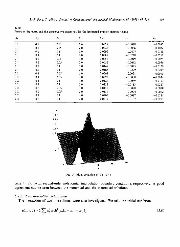
The parameters were taken to be K = 1.0, 2 = - l/v/-2 and x0 = 6.0 for the experiment, which was carried out on the domain [0, 20] x [0, 10]. The errors in the L~-norm and two of the conservatwe quantities Ii = f f u(x, y) dx dy and I2 = ½ f f u2(x, y) dx dy are computed and compared. Table 1 exhibits the results. Here, L~ = max [fit,m- ut,,,I, where fit.m and ut,,, are the numerical and the exact solutions, respectively, at the grid point (l,m). E1 =(71 -I~)/I~ and E2 =( /2 - I2) / I2 indicate the relative errors of the approximate values in the conserved quantities. Here [~ and 72 stand for the counterparts of I~ and 12, respectively, by the approximate solution of the KP equation. Simpson's rule was employed for the numerical quadrature of the integrals.

We assume that Table 1 shows an obedience of the conservation laws in the KP equation nu- merically. The profiles in Figs. 5 and 6 show the initial condition and the numerical solution at

B.-F Feng, T MitsuilJournal oJ Computattonal and Applied Mathematics 90 (1998) 95 116

Table 1 Errors m the norm and the conservatwe quantities for the hneanzed lmphclt method (2.18)

109

Ax Ay At t L~ E1 E2

0 0 0 0 0 0 0 0.1 0.2 02 0.2 02 02 0.2 02 0.2

0.1 0.05 1.0 0 0029 - 0 0019 -0.0033 0.1 0 05 2 0 0.0028 --0 0066 -0.0072 0.1 0 1 1.0 0 0090 0.0077 - 0 0185 0 1 0 1 2.0 0.0088 -00228 -0.0311 0 2 0.05 1.0 0.0050 -0.0019 - 0 0025 0 2 0.05 2.0 0.0052 -0.0062 -0.0056 0 2 0 1 1.0 0 0148 -0.0075 - 0 0176 0.2 0 1 2.0 0.0188 - 0 0229 -0.0299 0 1 0.05 1 0 0.0068 -0.0028 --0.0011 0 1 0.05 2 0 0 0090 -0.0008 --0.0054 0 1 0 1 1.0 0.0127 -0.0089 -0.0153 0 1 0.1 2.0 0 0132 -0.0183 -0.0227 0 2 0 05 1 0 0.0120 --0.0028 0.0018 0 2 0.05 2.0 0 0134 - 0 0004 0 0072 0.2 0 1 1 0 0 0205 --0 0087 - 0 0144 0 2 0 1 2.0 0 0239 - 0 0182 -0.0213

U

2

15

1

0.5

1 0 0

5 , v 0 x

20

Fig 5. lnitlal condition of Eq (5 4)

t ime t----2.0 (wi th second-order p o l y n o m i a l in terpola t ion b o u n d a r y condi t ion) , respect ively. A good

ag reemen t can be seen be tween the numer ica l and the theoret ical solut ions.

5.2.2. Two line-soliton interaction

The in terac t ion o f two l ine-so l i tons were also invest igated. We take the ini t ial cond i t ion

2

u(x, y, O) = 2 Z K2sech2 { tc,[x + )~,Y -- Xo,,]} t = l

(5 .6)

110 B.-F. Feng, T MitsutlJournal oJ Computattonal and Applied Mathemattcs 90 (1998) 95-116

l oo

L 0 5 10 1 20

0 x

Fig. 6. Numerical solution o f one hne-sohton at rime t = 2 0 (dx = 0.2, Ay = 0 2, At = 0 05)

and the exact boundary condition. We carried out the computation on the domain [0, 30] × [0, 3]. The initial condition (5.6) corresponds to two line-solitons, each with amplitude 2x~ placed initially at x =-x0,, and moving with velocity v, = 4x 2 -322 along the x-axis (i = 1,2). With a proper selection of the parameters, we can have positive and negative velocities to imply a collision of two line-soliton on the x - y plane.

The parameters /£1 ~ 1.0, /¢2 ~ 1/X/~, '~'1 ~ - l/x/3, '~'2 z - 1 . 0 , and x0,1 = 6 . 0 , x 0 , 2 - - 11.0 were taken for the numerical experiment from t = 0 to t = 4.5 allowing a collision to take place. The initial condition (5.6) is plotted in Fig. 7, which shows two wave pulses, with the larger on the left. As indicated above, the larger line-soliton on the left moves with a velocity 3.0 to the positive x-direction and the smaller one on the right moves with a velocity 1.0 to the negative x-direction. Consequently, as time goes on, these two line-solitons get close and collide with each other. Fig. 8 shows the profile at t = 3.0.

By t = 4.5, the two line-solitons have separated completely and restored their original shape. This is seen in Fig. 9.

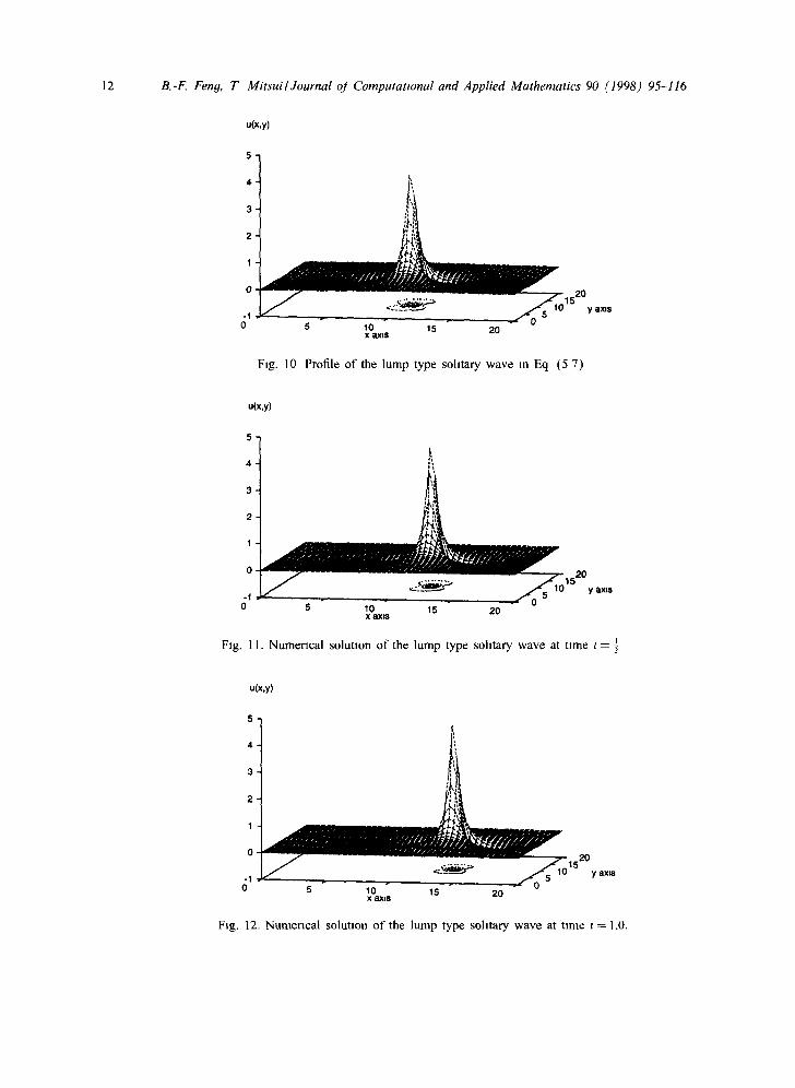
5.2.3. Lump type soliton The lump type initial conditions used for the KPI equation is

u ( x , y , O ) = 4 { _ ( x _Xo)2 + ~2(y _ yo)2 + 1/kt2} { ( x - Xo) 2 + ~ 2 ( y _ yo)2 + 1/p2} 2"

(5.7)

We adopt the boundary conditions (4.2) and (4.3) as discussed above. We computed in a rectangle [0, 20] x [0, 20] with the parameters /~2= 1.0,x0 = 10.0, Y0 = 10.0.

According to (1.3), this lump type pulse will move to the positive x-direction with velocity 3/t 2. Fig. 10 shows the initial condition of (5.7), while Figs. 10 and 11 give the numerical solution at

1 and t = 1.0, respectively. Stable propagation of the lump type solitary wave was observed times t = without any deformation.

B.-F. Feng, T M~lsuif Journa( oJ Computational and Apphed Mathematws 90 (1998) 95-116 111

25

2

15

1

0.5

5 10 15 20 25 30 X ax~s

Fig 7. lnmal condmon of Eq (5.6).

Y ax~s

2.5

2

1.5

0.~

C 0

Y axts

5 10 15 20 25 X axis

30

Fig 8. Numertcal solution of two hne-sohton interaction at t -- 3.0,

25

2

15

1

0.~

(

0

Fig

Y arts

$ lo 15 20 25 30 X ax~

9. Numerical solution of two hne-sohton interaction at t = 4 5.

12 B.-F, Fen9, T Mitsui/ Journal oJ Computattonal and Applied Mathematics 90 (1998) 95-116

u(x,y)

5-~

4 i ~

1 ¢~'- '<-~': '~ y axzs -1 j 5 1 0 1 5 2 0

r 0 0 5 I0 15 2O

x ~lS

Fig. 10 Profile of the lump type sohtary wave in Eq (5 7)

u(x,y)

5 -

4 -

3 -

2 -

1 -

0 5 10 15 20 x axis

1520 y ax is

I Fig. 11. Numerical solution of the lump type sohtary wave at time t =

u(x,y)

5

4

3 j i,

1

0 . ~ 0 1 0 1 5 2 0 <~.- '~ ~ y axts

- 1 . " ' r 0

0 5 10 15 20 x axis

F~g. 12. Numerical solution of the lump type sohtary wave at time t = 1.0.

B-F Fen9, T Mitsui l Journal oj Computational and Applied Mathemattcs 90 (1998) 95-116 113

U(x,y)

6

5

4

3

2

1

0

-1

0 5 10 15 20 25 30 35 x 8~xls

20

15

0 y axis

40

Fig. 13 Profile o f two lump type pulses at rime t = 0

Collision of two lump type solitary waves was also examined in the same way. We adopt the following initial conditions:

2 u(x, v , 0 ) = 4 ~ {-(x__- x0,,)_2_+_ #2(y~_ y0.,____)_2 _+_ 1//~ 2_____ ~

" ,=1 { ( X - - X 0 . , ) 2 + / . / 2 ( y _ y 0 . , ) 2 q_. 1 / / / 2 } 2 (5.8)

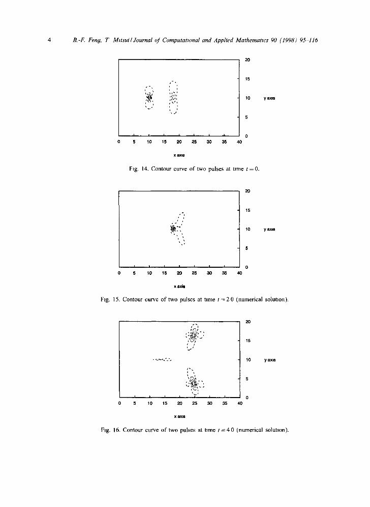
with the parameters: Xo.l = 10.0,x0,2 = 18.0, y0,1 =Yo.2 = 10.0,#~ = 1.5, /1~ =0.75. This is shown In Fig. 13. Recalling the lump type solitary wave solution of KPI equation in (1.3), the higher lump type soliton on the left will move with the velocity 4.5 in the positive x-direction, while the lower

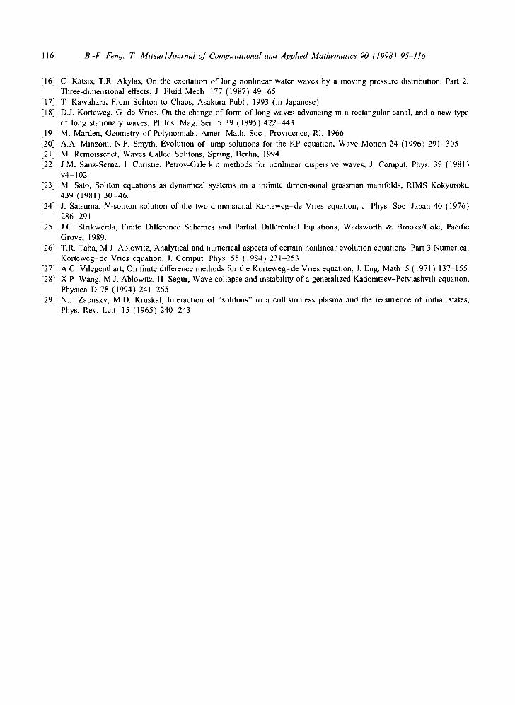
9 Hence, as time goes on, there will be one on the right moving in the same direction with velocity ~. a collision between two pulses. Because the pulse centers of the two localized pulses are situated on the same line with y = const., Kawahara called this kind of collision as "direct collision" [14]. Figs. 14-16 show the contour curves of the colliding pulses. It is very amazing that the pulses undergo "inelastic collision", i.e., they interact with each other and after the collision the amplitudes of pulses become almost equal, and the pulses move in the opposite direction along the y-axis, while keeping the total momentum be zero as before. The tipples observed in the figures have not yet reasonably explained. In the future, we are to pursue it numerically as well as analytically.

6. Summary and further aspects

A hnearized implicit finite difference method, based on the technique developed by Djidjeli, et al. [4], for the KdV equation was proposed. Moreover, the main work in the present paper is a direct and successful extension of this scheme to the KP equation. Analysis was carried out to the linearized implicit scheme for the both equations. It yielded the following merits.

(i) The order of accuracy was established as O ( ( A t ) 2 + (Ax) 2) and O((At) 2 + (Ax) 2, (Ay) 2) for the KdV and KP equations, respectively.

(ii) Unconditional linear stability was proven. (iii) Numerical dispersion was shown to be sufficiently small.

4 B.-F. Fen9, T MttsuilJournal oJ Computattonal and Applied Mathemattcs 90 (1998) 95-116

20

I

0 5

o I •

i t ~ J

~ ,J

I I ! I I I 0

10 15 20 25 30 35 40

15

10 yax=s

X a X I S

Fig. 14. Contour curve of two pulses at time t = O.

20

, ' 1

I I I I i I i 0

0 5 10 15 20 25 30 35 40

15

10 y axis

x ~ d l l

F]g. 15. Contour curve of two pulses at time t - - 2 0 (numerical solution).

t i i / . ' l i

• j,,,.ta~ - , ":,N"-' t

~ s i ¢

20

i ~ .

$ i

,¢S, ~ s

15

i I I I I 0

5 1 0 1 5 3 0 3 5 4 0

10 y axis

X ~ O I I

Fig. 16. Contour curve of two pulses at time t - - 4 0 (numerical solution).

B.-F Fen(4, T Mltsut/Journal oj Computattonal and Apphed Mathemattcs 90 (1998) 95 116 115

We carried out m a n y numerical computat ions with various initial conditions, most o f which are based on the analytical results via the inverse scattering transformation (IST). Numerical boundary conditions were proposed and partially justified through a theoretical analysis. The numerical re- sults were consistent with the theory and gave a good agreement to the analytical solutions. As a conclusion, our methods for the KdV and KP equations are effective. By applying our scheme to

the KP equation, the collision o f two lump type solitary pulses, whose behavior is still analytically unknown, was attained. This numerical experiment shows the powerfulness o f the numerical means

in the study o f nonlinear soliton equations. The two lump type solitary waves were observed to

undergo "inelastic collision", keeping the total m o m e n t u m conserved. The reason why the two lump

pulses behave so is an interesting topic we are to pursue for. A future work is expected to find a proper numerical boundary conditions for the general case

and to extend the linearized implicit method to the Zakharov-Kuzne t sov (ZK) equation, the Benney

equation and other mult i -dimensional soliton equations with nonlinear convective term.

Acknowledgements

The authors are very grateful to the anonymous referee for valuable comments and suggestions, which leads to an improvement on the earlier draft. We would also like to thank Professors T. Torii

and T. Kawahara for their helpful comments .

References

[1] M J Ablowltz, P A Clarkson, Sohtons, Nonhnear Evolution Equations and Inverse Scattering, Cambridge Umv Press, Cambndge, 1991.

[2] M J Ablowltz, J Vdlarroel, Solution to the ume dependent Schrodmger and the Kadomtsev-Petvlashvdl equations, Phys Rev Lea., to appear.

[3] A G. Bratsos, Ph.D Thesls, Brunel University, 1993, Chapter 5 [4] K Djldjefi, W G Pnce, E H Twlzell, Y. Wang, Numencal methods for the solution of the third- and fifth-order

dlsperswe Korteweg-de Vnes equations, J. Comput. Appl Math 58 (1995) 307 336 [5] B Fornberg, G.B. Whitham, A numencal and theoretical study of certain nonlinear wave phenomena, Phil Trans

Roy Soc London 289 (1978) 373-404. [6] N.C Freeman, J J C. Nlmmo, Sohton solutions of the Korteweg-de Vnes and the Kadomtsev-Petvlashvdl equations

the Wronsklan techmque, Proc Roy. Soc London A 389 (1983) 319-329. [7] N.C Freeman, Sohton solution of non-hnear evoluhon equation, IMA J Appl Math 32 (1984)125-145 [8] C S Gardner, J M Greene, M D. Kruskal, R M Mmra, Methods for solving the Kortweg-de Vnes equation, Phys

Rev Lett 19 (1967) 1095-1097 [9] C R Gdson, J.J.C. Nlmmo, Lump solutions of the BKP equation, Phys. Lett. A 147 (1990) 472-476

[10] B Gustafsson, H -O Krelss, J. Ohger, Time Dependent Problems and Difference Methods, Wiley, New York, 1995 [ll] K Goda, On mstablhty of some finite difference schemes for the Korteweg-de Vnes equation, J Phys Soc Japan

39 (1975) 229-236 [12] IS Grelg, J LL Morns, A hopscoth method for the Korteweg-de Vnes equation, J Comput Phys 20 (1976)

64 -80 [13] R Hlrota, Sohton Mathemahcs through Direct Method, iwanaml Publ, 1980 (m Japanese) [14] H lwasakl, S Toh, T Kawahara, Cyhndncal quas~-sohtons of the Zakharov-Kuznetsov equation, Physlca D 43

(1990) 293-303 [15] B B. Kadomtsev, V.I. Petwashvih, On the stabdlty of sohtary waves in a weakly dispersive medm, Soy Phys Dokl

15 (1970) 539 541

116 B-F Feng, T Mttsul/ Journal oJ Computattonal and Apphed Mathemattcs 90 (1998) 95-116

[16] C Katsls, T.R Akylas, On the excitation of long nonlinear water waves by a moving pressure distribution, Part 2, Three-dimensional effects, J Fluid Mech 177 (1987) 49-65

[17] T Kawahara, From Sohton to Chaos, Asakura Publ, 1993 (in Japanese) [18] D.J. Korteweg, G de Vrles, On the change of form of long waves advancing in a rectangular canal, and a new type

of long stationary waves, Phllos Mag. Ser 5 39 (1895) 422-443 [19] M. Marden, Geometry of Polynomials, Amer Math. Soc, Providence, RI, 1966 [20] A.A. Mmzonl, N.F. Smyth, Evolution of lump solutions for the KP equation, Wave Motion 24 (1996) 291-305 [21] M. Remolssenet, Waves Called Sohtons, Spring, Berlin, 1994 [22] J M. Sanz-Serna, I Christie, Petrov-Galerkln methods for nonlinear dispersive waves, J Comput. Phys. 39 (1981)

94-102. [23] M Sato, Sohton equations as dynamical systems on a infinite dimensional grassman manifolds, RIMS Kokyuroku

439 (1981) 30-46. [24] J. Satsuma, N-sohton solution of the two-dimensional Korteweg-de Vnes equation, J Phys Soc Japan 40 (1976)

286-291 [25] J C Stnkwerda, Finite Difference Schemes and Partial Differential Equations, Wadsworth & Brooks/Cole, Pacific

Grove, 1989. [26] T.R. Taha, M J Ablowltz, Analytical and numerical aspects of certain nonlinear evolution equations Part 3 Numerical

Korteweg-de Vries equation, J. Comput Phys 55 (1984) 231-253 [27] A C Vilegenthart, On finite difference methods for the Korteweg-de Vries equation, J. Eng. Math 5 (1971) 137-155 [28] X P Wang, M.J. Ablowitz, H Segur, Wave collapse and instability of a generalized Kadomtsev-Petvlashvlh equation,

Physica D 78 (1994) 241-265 [29] N.J. Zabusky, M D. Kruskal, Interaction of "sohtons" in a colhsionless plasma and the recurrence of initial states,

Phys. Rev. Lett 15 (1965) 240-243