WP/12/05

South African Reserve Bank Working Paper

A Financial Conditions Index for South Africa

Nombulelo Gumata, Nir Klein, Eliphas Ndou

Working Papers describe research in progress and are intended to elicit comments and contribute to debate. The views expressed are those of the author(s) and do not necessarily represent those of the South African Reserve Bank or Reserve Bank policy. While every precaution is taken to ensure the accuracy of information, the South African Reserve Bank shall not be liable to any person for inaccurate information or opinions contained herein.

South African Reserve Bank WP/12/05

South African Reserve Bank Working Paper Research Department

Prepared by Nombulelo Gumata, Nir Klein, Eliphas Ndou

Authorised for internal distribution by Dr L C Loewald

August 2012

Abstract

The main purpose of this paper is to construct a financial conditions index (FCI) forSouth Africa. The analysis extracts the index by applying two alternative approaches(principal component analysis and Kalman filter), which identify an unobservablecommon factor from a group of external and domestic financial indicators. Thealternative estimated FCIs, which share a similar trajectory over time, seem to have powerful predictive information for the near-term gross domestic product (GDP)growth (up to four quarters), and they outperform the South African Reserve Bank’s(SARB) leading indicator, as well as individual financial variables. Their recentdynamics suggest that following a strong recovery in late 2009 and 2010, reflecting in part domestic factors such as systematic reductions in the policy rate, the rebound in real economic activity and a benign inflationary environment, the financialconditions have deteriorated in recent months, though not as sharply as in end-2008. Given their relatively high predictive power regarding GDP growth, a further deterioration may imply that economic activity is likely to slow in the period ahead. JEL classification: E5, E17, E44 Keywords: Financial conditions index, factor analysis Corresponding author’s e-mail address: Nombulelo.Gumata@resbank.co.za; nklein@imf.org; Eliphas.Ndou@resbank.co.za

Table of Contents

1 Introduction ............................................................................................................................. 3

2 Principal Component Approach (PCA) .................................................................................... 5

3 Extracting the Common Factor by a Kalman Filter .................................................................. 8

4 The Estimated Financial Conditions Indices: A Comparison ................................................... 9 5 Evaluation of the financial indices ......................................................................................... 12

6 What Can the Financial Conditions Index Tell About the Near-Term GDP Growth? ............. 17

7 Conclusion ............................................................................................................................ 20

References ........................................................................................................................................ 21

Appendix ............................................................................................................................................ 22 Figure 1 Factor Loadings ..................................................................................................................... 7 Figure 2. The Estimated Financial Conditions Indices (FCIs) ............................................................. 10 Figure 3. The Estimated FCIs Scaled by the Sample Standard Deviations ........................................ 11 Figure 4. Demeaned GDP Growth and the Alternative FCIs .............................................................. 16 Figure 5. Static Forecast, 2008q1–2011q4 ........................................................................................ 17 Figure 6. Dynamic Forecast, 2012q1-2012q4 .................................................................................... 19 Table 1 Granger Causality tests of Alternative FCIs and GDP ........................................................... 13 Table 2 The Explanatory Power of the Indices ................................................................................... 14 Table 3 Comparison of SSR for 1,2, and 4 Quarters Ahead, ............................................................. 15 Table 4 The Predictive Power of the Indices ...................................................................................... 17 Table 5. Forecast Results under Three Scenarios ............................................................................. 19

3

1. Introduction

The response of real economic activity to the recent global financial crisis and the

ongoing sovereign debt crisis highlighted the importance of macro-financial linkages

and demonstrated how severe the impact of financial markets’ stress on real activity

can be. But more generally, financial conditions are known to have an important

influence on business cycles because they reflect not only the feedback of current

and past economic conditions, but also the markets’ expectations about the

economic outlook. Thus, the assessment of the financial conditions on an ongoing

basis has become critical for policy-makers, regulators, market financial participants,

and researchers, who have increasingly worked to construct financial conditions

indices that can be used as operational tools to better understand the macro-

financial linkages and also to obtain a historical perspective in comparing the relative

tightness or looseness of financial conditions.

A wide range of methodologies for constructing the financial conditions indices have

been developed over time, but the most popular are the weighted-sum approach and

the principal component approach.1 In the first approach, the weights of each

financial indicator are assigned according to the estimated impact on real GDP

growth in a vector autoregressive (VAR) or structural macroeconomic models.2 In

the second approach, the financial conditions index (FCI) reflects a common factor,

which is extracted from a group of financial indicators and captures the greatest

common variation among them.3 The models in this group differ by the estimation

1 Hatzius and others (2010) provide an extensive survey on financial conditions indices, which were constructed in recent years.

2 Examples of a weighted-sum approach are the FCIs of the Organisation of Economic Co-operation and Development (OECD), Goldman Sachs, Bloomberg and Citigroup. In South Africa, the Quantec financial conditions index regresses real short-term interest rates, the yield spread, excess money supply growth, company earnings yield, and the real effective exchange rate on manufacturing production. Each variable’s coefficients are then used to give an approximation of the relative weights.

3 Such indices are used by Deutsche Bank and the Federal Reserve Bank of Kansas City.

4

methods and by the statistical processes, in which the unobserved common factor is

specified.

This paper aims to construct an FCI for South Africa, which can be used as a

leading indicator for short-term economic activity and as a tool to assess financial

conditions across time. The analysis uses the methodology proposed by Hatzius and

others (2010) and applied in Osorio, Pongsaparn and Unsal (2011). This approach

strips the unobservable principal component factor from the feedback of economic

activity. Acknowledging the limitations of the principal component approach, the

analysis also applies an alternative methodology, Kalman filter, which provides the

estimated FCI with greater auto-correlation over time.

The results show that the financial conditions started deteriorating in 2007Q3 and

worsened in 2008, and ultimately affected real economic activity. While recovering

strongly in late 2009 and 2010, the financial conditions have tightened in recent

months, although not as sharply as in 2008. Moreover, the estimated FCIs were

found to have powerful predictive information for near-term GDP growth by up to

four quarters and outperform the current SARB leading indicator as well as other

individual financial indicators. Based on this, the recent deterioration in the financial

condition indices suggests that economic activity in South Africa is likely to moderate

in the period ahead.

This paper is structured as follows: Section II describes the principal component

approach (PCA) and presents the financial indicators used to construct the FCI

under this methodology. Section III offers an alternative approach (Kalman filter),

which allows for auto-correlation and thus gives the estimated FCI greater dynamics

over time. Section IV looks at the alternative indices and compares their evolution

over time; Section V evaluates the financial conditions indices by performing

Granger causality tests and by looking at the explanatory power for near-term GDP

growth and compares them to that of the SARB’s leading indicator; Section VI

assesses the impact of the recent deterioration of the financial conditions on GDP

5

growth by presenting dynamic simulations under three different scenarios for 2012.

Section VII concludes.

2. Principal Component Approach (PCA)

The principal component methodology aims at extracting a common factor that

captures the greatest common variation in a group of P variables . Analytically,

the model can be presented as follows:4

(1)

Where is a 1vector of the variables’ means. is a matrix of coefficients,

and is a vector of 1 unobserved variables, termed as common factors, and

is a 1vector of errors. The model assumes that errors are orthogonal to the

common factors, [ ′ 0 , and that the common factors have zero mean 0. We calculate a common factor for the period of 1999q1 and 2011q4 based on both

financial indicators that are entirely exogenous to South Africa and reflect the global

financial conditions as well as indicators that relate specifically to South Africa. The

variables selected cover measures of market risk and liquidity, with implications for

monetary policy, financial stability and economic activity.

The variables are divided into global and domestic factors. The global factors include

the S&P500 volatility index (VIX), which reflects international investors’ appetite for

risk; S&P500 stock price index (SP500) indicates general market risk; JP Morgan

EMBI total return index (EMBI) is a measure of risk aversion and tracks returns for

actively traded external emerging market debt; and the spread between the three-

month LIBOR and the yield on a three-month US Treasury Bill (TED), which

4 The main benefit of the principal component approach (PCA) is its ability to determine the individual importance of a large number of indicators so that the weight allocated to each indicator is consistent with its historical importance to fluctuations in the broader financial system. For extensive discussion on the PCA, see Johnson and Wichern (1992).

6

measures the perceived credit risk, global liquidity conditions and uncertainty

surrounding the projected path of US monetary policy.

The domestic (South Africa related) indicators are: total loans and advances to the

private sector (LOANS_ADV) that capture the demand factors affecting the

economic outlook and supply constraints not captured by interest rates; the South

African sovereign spread (SOVEREIGN) indicates risk of the government’s funding

ability in the capital markets, non-performing loans (NPL) indicate the health of the

banking sector and the building up of risks in the banking sector; the negotiable

certificates of deposit rate (NCD) measures the cost of financing for firms and

households; the nominal effective exchange rate (NEER) captures the magnitude of

capital flows to and from South Africa; the all-share Johannesburg Stock Exchange

index (JSE); and the ABSA house price index (ABSA), which captures asset prices,

the wealth and collateral channels, and expectations about inflation and other

macroeconomic conditions.5

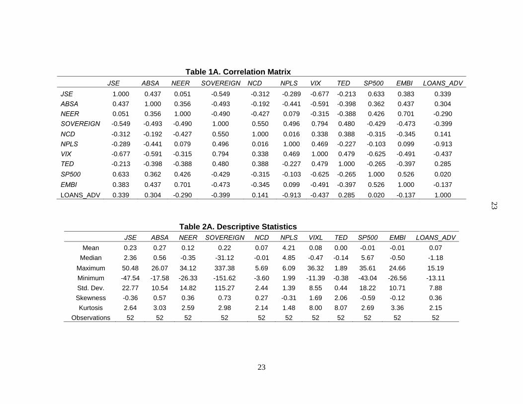
While many variables were considered in the first round, the selection of the final

variables was based on their factor “loadings”, i.e., correlation coefficients. For this

exercise, we set the threshold at 30 percent. All variables are demeaned and

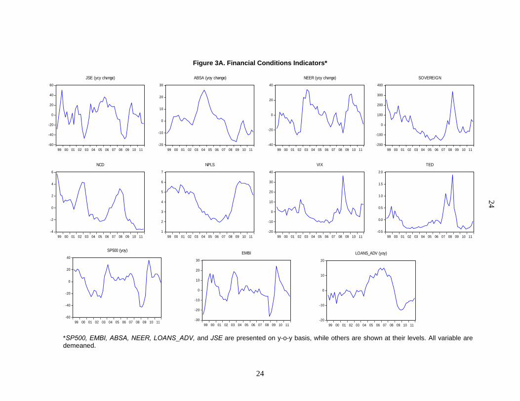
transformed to I(0). In this regard, the variables NEER, JSE, ABSA, LONS_ADV,

EMBI, and SP500 are measured on a y-o-y basis while the rest of the variables are

measured at their levels (Figure 3A in the appendix).

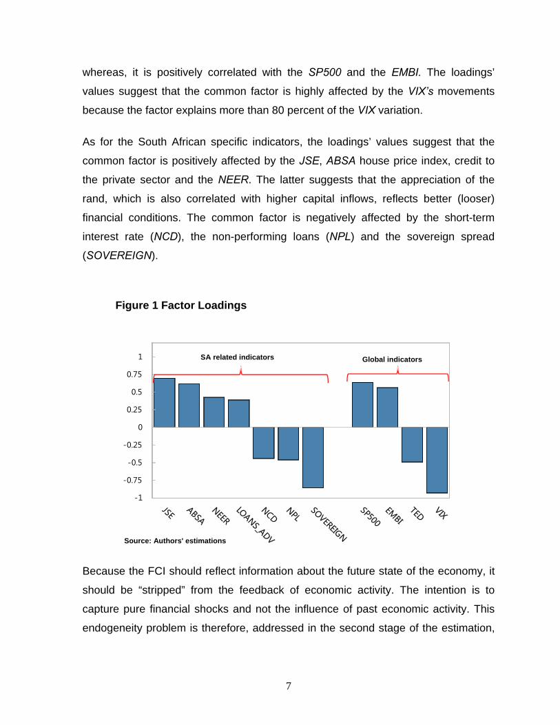
Figure 1 shows the factors “loadings”. These loadings reveal the signs and

magnitudes of variables included in the index. The signs and magnitudes are

important in capturing and assessing the systematic relationships with the identified

common factor. The more correlated the factor is with other variables, the higher the

allocated weight. In particular, Figure 1 shows that, among the global indicators, the

common factor is negatively correlated with the VIX and the TED movements, 5 It is worth noting that despite the emphasized importance of the inclusion of credit availability surveys in the construction of FCIs in the literature, we are not able to include such qualitative variables in our index because the available series only start in 2002 Q1.

7

whereas, it is positively correlated with the SP500 and the EMBI. The loadings’

values suggest that the common factor is highly affected by the VIX’s movements

because the factor explains more than 80 percent of the VIX variation.

As for the South African specific indicators, the loadings’ values suggest that the

common factor is positively affected by the JSE, ABSA house price index, credit to

the private sector and the NEER. The latter suggests that the appreciation of the

rand, which is also correlated with higher capital inflows, reflects better (looser)

financial conditions. The common factor is negatively affected by the short-term

interest rate (NCD), the non-performing loans (NPL) and the sovereign spread

(SOVEREIGN).

Figure 1 Factor Loadings

Because the FCI should reflect information about the future state of the economy, it

should be “stripped” from the feedback of economic activity. The intention is to

capture pure financial shocks and not the influence of past economic activity. This

endogeneity problem is therefore, addressed in the second stage of the estimation,

-1

-0.75

-0.5

-0.25

0

0.25

0.5

0.75

1

Source: Authors' estimations

SA - related indicators Global indicators

8

when we purge the estimated common factor of this feedback by regressing on

current GDP growth ( ) as follows:

(2) Where is uncorrelated with . We can now refer to as the estimated FCI, which

reflects only the exogenous shifts in the financial conditions and thus should have a

predictive power for future economic activity.6 This will be examined in subsequent

sections.

3. Extracting the Common Factor by a Kalman Filter

One of the main drawbacks of the principal component estimator is that the factor is

constructed as a stationary variable with a zero mean, thus it lacks a dynamic

(autocorrelation) pattern, which, in the context of estimating an FCI, is important

given that the aim is to predict the near-term GDP growth, which, in general, is

characterised by more gradual shifts. Therefore, in this section we expand the factor

structure to include a more dynamic specification. This is done by using the following

state-space form:

(3) (4) Where Eq. (3) is the signal equation that includes the vector of the observable

variables, , their mean, , and the estimated common factor, . Eq. (4) is the state

equation, which describes the statistical process of the estimated common factor.

Here, we simultaneously strip the observable variables from the feedback of

economic activity by including the current GDP growth in the signal equation. The

error terms and are independent disturbances with zero mean.

6 The unpurged factor is presented in Figure 1A in the appendix.

9

For comparison, we used the same set of financial indicators in both methodologies

to construct the financial conditions indices. The comparison of the dynamics of the

two alternative FCIs is presented in the next section.

4. The Estimated Financial Conditions Indices: A Comparison

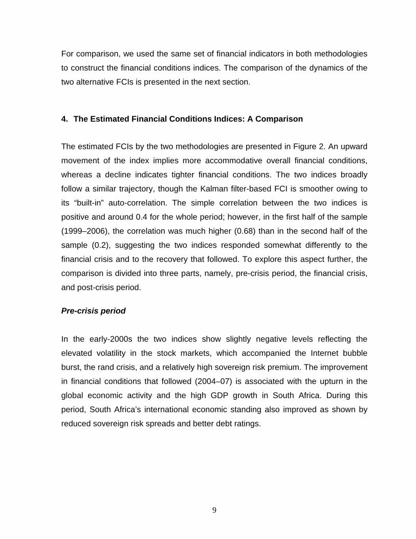
The estimated FCIs by the two methodologies are presented in Figure 2. An upward

movement of the index implies more accommodative overall financial conditions,

whereas a decline indicates tighter financial conditions. The two indices broadly

follow a similar trajectory, though the Kalman filter-based FCI is smoother owing to

its “built-in” auto-correlation. The simple correlation between the two indices is

positive and around 0.4 for the whole period; however, in the first half of the sample

(1999–2006), the correlation was much higher (0.68) than in the second half of the

sample (0.2), suggesting the two indices responded somewhat differently to the

financial crisis and to the recovery that followed. To explore this aspect further, the

comparison is divided into three parts, namely, pre-crisis period, the financial crisis,

and post-crisis period.

Pre-crisis period

In the early-2000s the two indices show slightly negative levels reflecting the

elevated volatility in the stock markets, which accompanied the Internet bubble

burst, the rand crisis, and a relatively high sovereign risk premium. The improvement

in financial conditions that followed (2004–07) is associated with the upturn in the

global economic activity and the high GDP growth in South Africa. During this

period, South Africa’s international economic standing also improved as shown by

reduced sovereign risk spreads and better debt ratings.

10

Financial crisis period

During the financial crisis and the period that followed, the PCA-based FCI seems to

exhibit sharper swings: it deteriorated faster than the Kalman filter-based FCI as it

reached its low point of -3.2 already in 2008q4, and it recovered quite strongly in the

subsequent quarters, reaching its high point in 2009q4. The Kalman filter-based FCI

seems to react two quarters later to the financial crisis as it reached its record-low

level in 2009q2.

Figure 2. The Estimated Financial Conditions Indices (FCIs)

Post-crisis period

The Kalman filter-based FCI also recovered more gradually than the PCA-based

FCI, and its level in the post-crisis period remained below its pre-crisis level. While

the PCA-based FCI showed a gradual deterioration in 2010 and 2011, entering

negative territory in recent months, the Kalman filter-based index remained flat from

-3.5

-2.5

-1.5

-0.5

0.5

1.5

2.5

1999Q1 2000Q3 2002Q1 2003Q3 2005Q1 2006Q3 2008Q1 2009Q3 2011Q1

FCI by Kalman filter

FCI by PCA

Source: Authors' estimates.

Tighter conditions

Looserconditions

11

2010q2 to 2011q3. In 2011q4, however, it has somewhat deteriorated to just below

zero.

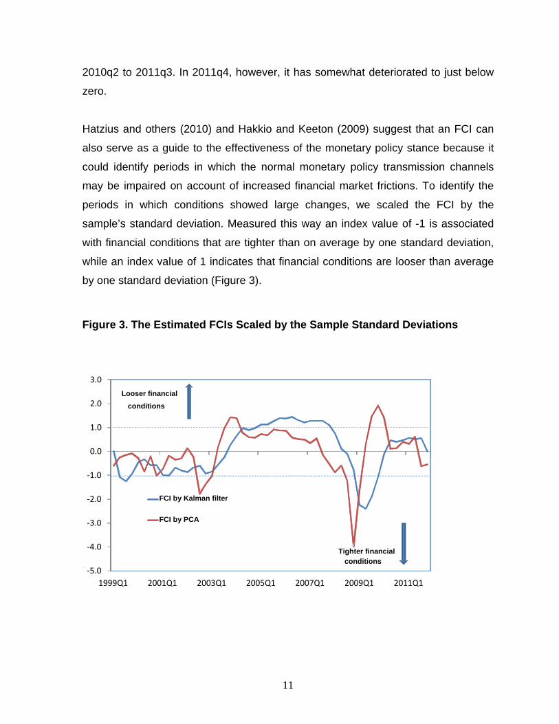
Hatzius and others (2010) and Hakkio and Keeton (2009) suggest that an FCI can

also serve as a guide to the effectiveness of the monetary policy stance because it

could identify periods in which the normal monetary policy transmission channels

may be impaired on account of increased financial market frictions. To identify the

periods in which conditions showed large changes, we scaled the FCI by the

sample’s standard deviation. Measured this way an index value of -1 is associated

with financial conditions that are tighter than on average by one standard deviation,

while an index value of 1 indicates that financial conditions are looser than average

by one standard deviation (Figure 3).

Figure 3. The Estimated FCIs Scaled by the Sample Standard Deviations

Looser financial

conditions

Tighter financial conditions

- 5.0

- 4.0

- 3.0

- 2.0

- 1.0

0.0

1.0

2.0

3.0

1999Q1 2001Q1 2003Q1 2005Q1 2007Q1 2009Q1 2011Q1

FCI by Kalman filter

FCI by PCA

12

Figure 3 indicates looser conditions that exceed one standard deviation in 2003q3 to

2004q2 and 2009q3 to 2010q1 whereas the dynamic Kalman filter FCI points

2004q1 to 2007q4. That said, the PCA and Kalman FCIs indicate that financial

conditions were significantly tighter and exceeded one standard deviation in 2008Q3

to 2009Q1 and 2009q1 to 2009q4, respectively. This may suggest that the

deterioration in financial conditions during these periods was not conducive for

efficient/effective transmission of monetary policy changes through certain traditional

channels.

In particular, during this period, house prices plummeted by a larger proportion than

historic averages, stock prices lost significant value, non-performing loans and other

measures of impaired loans and advances outside the banking sector increased,

and credit extension to the private sector shrank significantly. The high illiquidity of

disposable assets and price devaluation weakened the role of the wealth and

collateral channels in facilitating access to credit and thereby possibly adding

frictions to already imperfect markets and further impairing the transmission of

monetary policy changes into the real economy. Although not at a significant level,

the latest deteriorations coincide with lingering European sovereign debt problems,

which affect sovereign risk and risk appetite.

5. Evaluation of the financial indices

This section conducts various tests to ascertain the effectiveness of financial

conditions indices as a policy tool by performing Granger causality tests and two

forecasting exercises. First, we conduct Granger causality tests of the two

alternative FCIs and GDP. Second, we evaluate and determine which of the

estimated FCIs has greater ability to explain and predict GDP growth over the near-

term, and compare it to that of the SARB’s composite leading business cycle

13

indicator.7 Third, we assess the relative predictive performance of the FCI to various

variables included in the index.

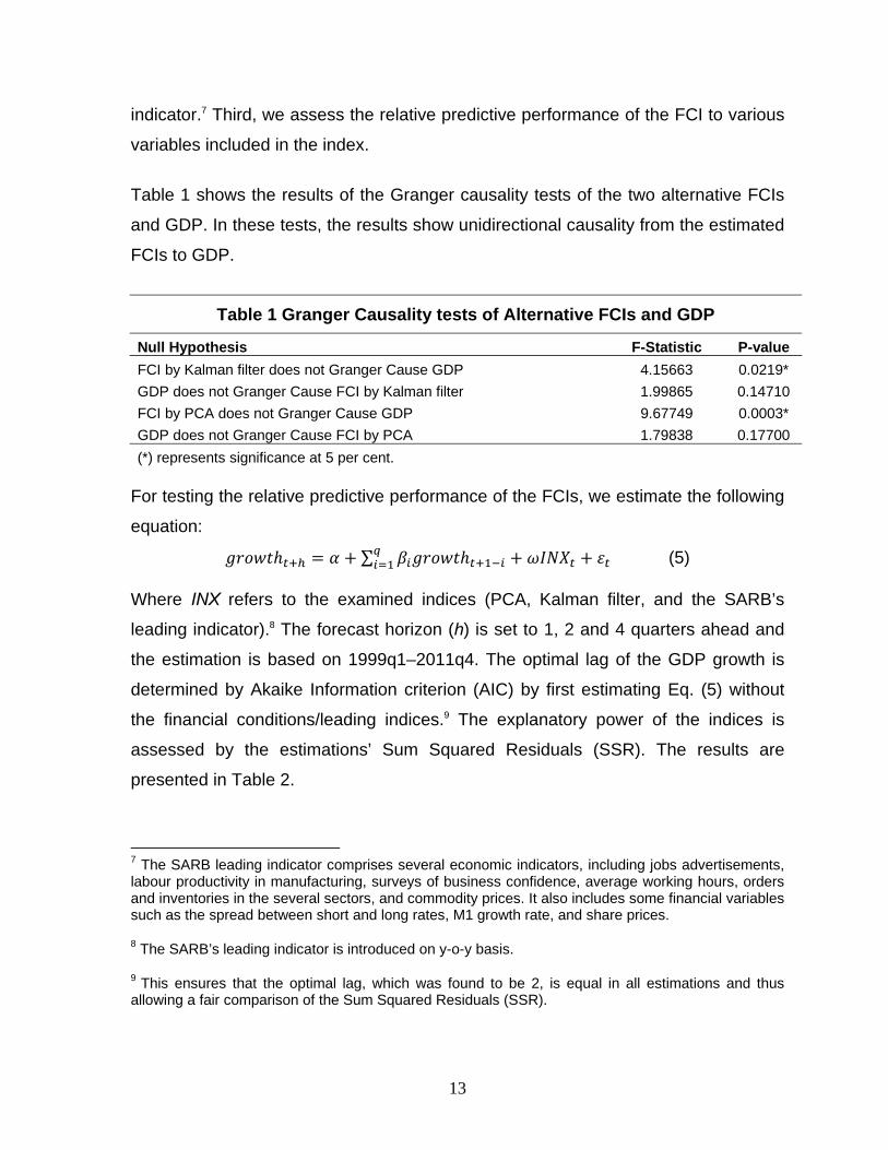
Table 1 shows the results of the Granger causality tests of the two alternative FCIs

and GDP. In these tests, the results show unidirectional causality from the estimated

FCIs to GDP.

Table 1 Granger Causality tests of Alternative FCIs and GDP

Null Hypothesis F-Statistic P-value

FCI by Kalman filter does not Granger Cause GDP 4.15663 0.0219*

GDP does not Granger Cause FCI by Kalman filter 1.99865 0.14710

FCI by PCA does not Granger Cause GDP 9.67749 0.0003*

GDP does not Granger Cause FCI by PCA 1.79838 0.17700

(*) represents significance at 5 per cent. For testing the relative predictive performance of the FCIs, we estimate the following

equation: ∑ (5) Where INX refers to the examined indices (PCA, Kalman filter, and the SARB’s

leading indicator).8 The forecast horizon (h) is set to 1, 2 and 4 quarters ahead and

the estimation is based on 1999q1–2011q4. The optimal lag of the GDP growth is

determined by Akaike Information criterion (AIC) by first estimating Eq. (5) without

the financial conditions/leading indices.9 The explanatory power of the indices is

assessed by the estimations’ Sum Squared Residuals (SSR). The results are

presented in Table 2.

7 The SARB leading indicator comprises several economic indicators, including jobs advertisements, labour productivity in manufacturing, surveys of business confidence, average working hours, orders and inventories in the several sectors, and commodity prices. It also includes some financial variables such as the spread between short and long rates, M1 growth rate, and share prices.

8 The SARB’s leading indicator is introduced on y-o-y basis.

9 This ensures that the optimal lag, which was found to be 2, is equal in all estimations and thus allowing a fair comparison of the Sum Squared Residuals (SSR).

14

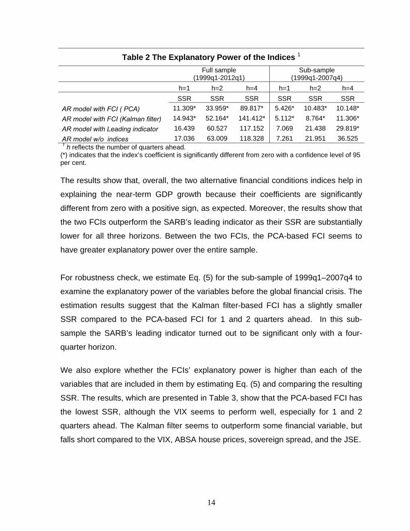
Table 2 The Explanatory Power of the Indices 1

Full sample (1999q1-2012q1)

Sub-sample (1999q1-2007q4)

h=1 h=2 h=4 h=1 h=2 h=4

SSR SSR SSR SSR SSR SSR

AR model with FCI ( PCA) 11.309* 33.959* 89.817* 5.426* 10.483* 10.148*

AR model with FCI (Kalman filter) 14.943* 52.164* 141.412* 5.112* 8.764* 11.306*

AR model with Leading indicator 16.439 60.527 117.152 7.069 21.438 29.819*

AR model w/o indices 17.036 63.009 118.328 7.261 21.951 36.525 1 h reflects the number of quarters ahead. (*) indicates that the index’s coefficient is significantly different from zero with a confidence level of 95 per cent.

The results show that, overall, the two alternative financial conditions indices help in

explaining the near-term GDP growth because their coefficients are significantly

different from zero with a positive sign, as expected. Moreover, the results show that

the two FCIs outperform the SARB’s leading indicator as their SSR are substantially

lower for all three horizons. Between the two FCIs, the PCA-based FCI seems to

have greater explanatory power over the entire sample.

For robustness check, we estimate Eq. (5) for the sub-sample of 1999q1–2007q4 to

examine the explanatory power of the variables before the global financial crisis. The

estimation results suggest that the Kalman filter-based FCI has a slightly smaller

SSR compared to the PCA-based FCI for 1 and 2 quarters ahead. In this sub-

sample the SARB’s leading indicator turned out to be significant only with a four-

quarter horizon.

We also explore whether the FCIs’ explanatory power is higher than each of the

variables that are included in them by estimating Eq. (5) and comparing the resulting

SSR. The results, which are presented in Table 3, show that the PCA-based FCI has

the lowest SSR, although the VIX seems to perform well, especially for 1 and 2

quarters ahead. The Kalman filter seems to outperform some financial variable, but

falls short compared to the VIX, ABSA house prices, sovereign spread, and the JSE.

15

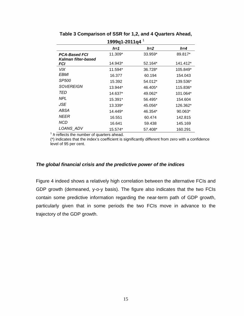
Table 3 Comparison of SSR for 1,2, and 4 Quarters Ahead,

1999q1-2011q4 1

h=1 h=2 h=4

PCA-Based FCI 11.309* 33.959* 89.817* Kalman filter-based FCI 14.943* 52.164* 141.412*

VIX 11.594* 36.728* 105.849* EBMI 16.377 60.194 154.043 SP500 15.392 54.012* 139.536* SOVEREIGN 13.944* 46.405* 115.836* TED 14.637* 49.062* 101.064* NPL 15.391* 56.495* 154.604 JSE 13.339* 45.056* 126.362* ABSA 14.449* 46.354* 90.063* NEER 16.551 60.474 142.815 NCD 16.641 59.438 145.169 LOANS_ADV 15.574* 57.408* 160.291

1 h reflects the number of quarters ahead. (*) indicates that the index’s coefficient is significantly different from zero with a confidence level of 95 per cent.

The global financial crisis and the predictive power of the indices

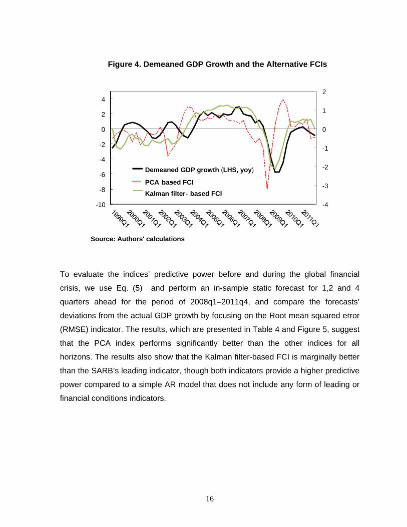
Figure 4 indeed shows a relatively high correlation between the alternative FCIs and

GDP growth (demeaned, y-o-y basis). The figure also indicates that the two FCIs

contain some predictive information regarding the near-term path of GDP growth,

particularly given that in some periods the two FCIs move in advance to the

trajectory of the GDP growth.

16

Figure 4. Demeaned GDP Growth and the Alternative FCIs

To evaluate the indices’ predictive power before and during the global financial

crisis, we use Eq. (5) and perform an in-sample static forecast for 1,2 and 4

quarters ahead for the period of 2008q1–2011q4, and compare the forecasts’

deviations from the actual GDP growth by focusing on the Root mean squared error

(RMSE) indicator. The results, which are presented in Table 4 and Figure 5, suggest

that the PCA index performs significantly better than the other indices for all

horizons. The results also show that the Kalman filter-based FCI is marginally better

than the SARB’s leading indicator, though both indicators provide a higher predictive

power compared to a simple AR model that does not include any form of leading or

financial conditions indicators.

- 4

- 3

- 2

- 1

0

1

2

- 10

- 8

- 6

- 4

- 2

0

2

4

Demeaned GDP growth (LHS, yoy)

PCA -based FCI

Kalman filter- based FCI

Source: Authors' calculations

17

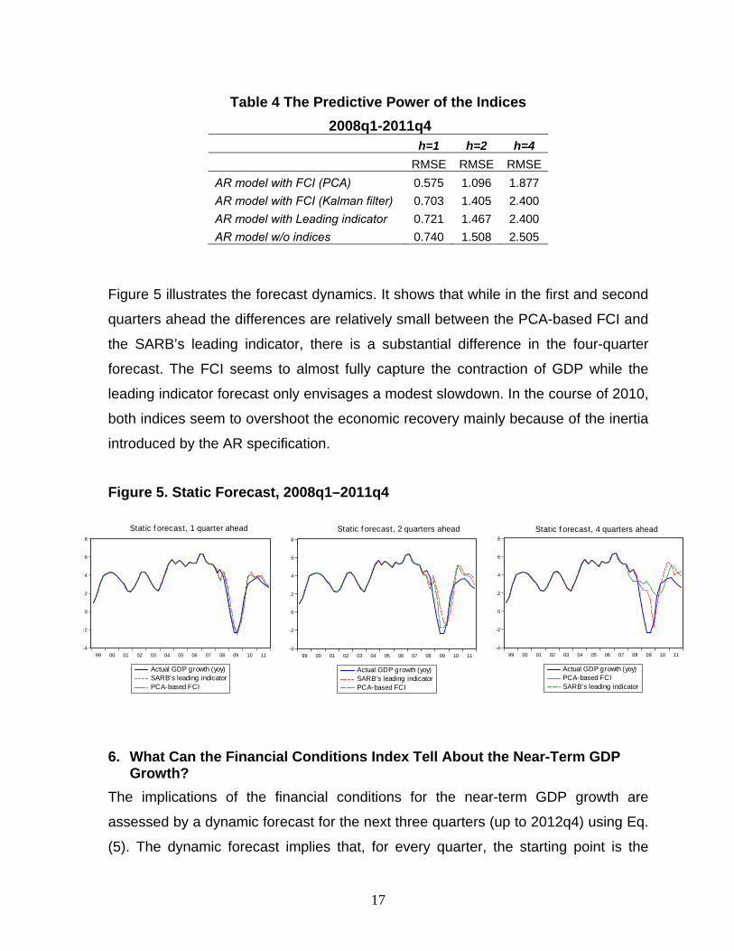
Table 4 The Predictive Power of the Indices

2008q1-2011q4

h=1 h=2 h=4

RMSE RMSE RMSE

AR model with FCI (PCA) 0.575 1.096 1.877

AR model with FCI (Kalman filter) 0.703 1.405 2.400

AR model with Leading indicator 0.721 1.467 2.400

AR model w/o indices 0.740 1.508 2.505

Figure 5 illustrates the forecast dynamics. It shows that while in the first and second

quarters ahead the differences are relatively small between the PCA-based FCI and

the SARB’s leading indicator, there is a substantial difference in the four-quarter

forecast. The FCI seems to almost fully capture the contraction of GDP while the

leading indicator forecast only envisages a modest slowdown. In the course of 2010,

both indices seem to overshoot the economic recovery mainly because of the inertia

introduced by the AR specification.

Figure 5. Static Forecast, 2008q1–2011q4

6. What Can the Financial Conditions Index Tell About the Near-Term GDP Growth?

The implications of the financial conditions for the near-term GDP growth are

assessed by a dynamic forecast for the next three quarters (up to 2012q4) using Eq.

(5). The dynamic forecast implies that, for every quarter, the starting point is the

-4

-2

0

2

4

6

8

99 00 01 02 03 04 05 06 07 08 09 10 11

Actual GDP growth (yoy)PCA-based FCISARB's leading indicator

Static f orecast, 4 quarters ahead

-4

-2

0

2

4

6

8

99 00 01 02 03 04 05 06 07 08 09 10 11

Actual GDP growth (yoy)SARB's leading indicatorPCA-based FCI

Static f orecast, 2 quarters ahead

-4

-2

0

2

4

6

8

99 00 01 02 03 04 05 06 07 08 09 10 11

Actual GDP growth (yoy)SARB's leading indicatorPCA-based FCI

Static f orecast, 1 quarter ahead

18

model’s prediction. For this exercise we use the FCI under the principal component

approach, which was found to outperform the Kalman filter-FCI and the SARB’s

leading indicator. In light of the ongoing sovereign crisis in the euro-area and the

potential repercussions on South Africa’s financial conditions, we focus on three

main scenarios for the remainder of the year.10 The first scenario assesses the

impact of current financial conditions (2012q1) while the last two scenarios focus on

tighter or more restrictive financial conditions. The assumed three scenarios are:

1. Financial conditions remain at their current level (as of 2012q1) throughout

the forecast horizon (0.5).

2. Financial conditions gradually deteriorate, and return to the average level

of the second half of 2011 (-0.5).

3. Financial conditions sharply deteriorate and reach the average level that

was observed in 2008 (-1.4).

The FCI trajectories under the three scenarios and the dynamic forecasts are

presented in Figure 6. While the impact on GDP growth largely depends on both the

magnitude and the pace at which the financial conditions deteriorate, the forecast

results suggest that they have a substantial effect on economic activity. More

specifically, under the “no change” scenario, GDP growth is projected to accelerate

gradually to 3.4 percent in 2012q4, suggesting that the average 2012 GDP growth

will be 2.7 percent, which is consistent with the growth projection of the 2012 budget.

10 For this exercise, we updated the FCI using the 2012q1 GDP figure that was published at end-May 2012.

19

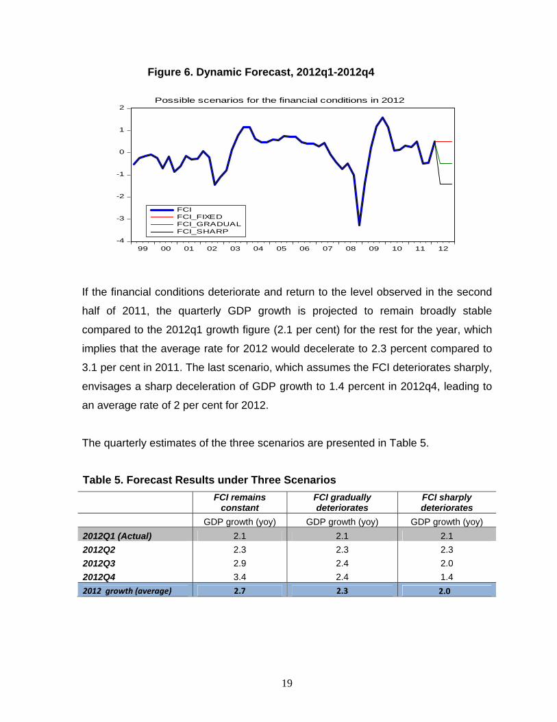
Figure 6. Dynamic Forecast, 2012q1-2012q4

If the financial conditions deteriorate and return to the level observed in the second

half of 2011, the quarterly GDP growth is projected to remain broadly stable

compared to the 2012q1 growth figure (2.1 per cent) for the rest for the year, which

implies that the average rate for 2012 would decelerate to 2.3 percent compared to

3.1 per cent in 2011. The last scenario, which assumes the FCI deteriorates sharply,

envisages a sharp deceleration of GDP growth to 1.4 percent in 2012q4, leading to

an average rate of 2 per cent for 2012.

The quarterly estimates of the three scenarios are presented in Table 5.

Table 5. Forecast Results under Three Scenarios

FCI remains constant

FCI gradually deteriorates

FCI sharply deteriorates

GDP growth (yoy) GDP growth (yoy) GDP growth (yoy)

2012Q1 (Actual) 2.1 2.1 2.1

2012Q2 2.3 2.3 2.3

2012Q3 2.9 2.4 2.0

2012Q4 3.4 2.4 1.4

2012 growth (average) 2.7 2.3 2.0

-4

-3

-2

-1

0

1

2

99 00 01 02 03 04 05 06 07 08 09 10 11 12

FCIFCI_FIXEDFCI_GRADUALFCI_SHARP

Possible scenarios for the financial conditions in 2012

20

7. Conclusion

The paper constructs FCIs for South Africa. The analysis extracts the index by

applying two alternative approaches, namely, the principal component analysis and

Kalman filter, which identify an unobservable common factor from a group of

external and domestic financial indicators. We tested the predictive power of the FCI

using out-of-sample and an in-sample forecasting exercise. This forecasting

exercise compares the performance of both FCIs against the autoregressive model

of GDP growth, the SARB’s leading indicator, and the predictive capacity of various

key financial market variables at one, two, and four quarters ahead.

The results indicate that both the PCA and Kalman filtered FCIs performed better as

leading indicators of real economic activity relative to the SARB’s leading indicator,

and to an autoregressive model of GDP growth. The PCA-based FCI also

outperforms the individual financial indicators that it includes. These findings suggest

that joint movements in financial variables effectively contain relevant information

regarding future outcomes in real activity. Among the two alternative FCIs, the PCA-

based FCI seems to have greater explanatory power over the entire sample, though

during the pre-crisis period, the Kalman filter-based FCI seems to have performed

better in predicting GDP growth, particularly for one and two quarters ahead.

The dynamics of the FCIs suggest that, following a strong recovery in late-2009 and

2010, the financial conditions have deteriorated in recent months, though not as

sharply as in 2008. Because the estimated FCIs were found to have powerful

predictive information for the near-term GDP growth (up to four quarters), further

deterioration may imply that economic activity is likely to slow in the period ahead.

21

References

Akerli, A., A. Zadornova, and J. Pinder. 2010. “Financial Conditions Signal Growth Divergence in the New markets”, Goldman Sachs New Market Analyst, No. 10/01. Beaton, K., R. Lalonde, and C. Luu. 2009. “A Financial Conditions Index for the United States”, Bank of Canada Discussion paper 2009–11. Brave, S. and R. A Butters. 2010. “Gathering insights on the forest from the trees: A new metric for financial conditions”, Working Paper 2010-07, Federal Reserve of Chicago. Chamberlain, G. and M. Rothschild. 1983. “Arbitrage, Factor Structure and Mean Variance Analysis on Large Asset Markets”, Econometrica, No. 51, 1305–24. Dudley, W. C. 2010. “Comments on Financial Conditions Indexes: A New Look after the Financial Crisis”, Remarks at the University of Chicago Booth School of Business Annual U.S. Monetary Policy Forum, New York City (February 26). Hatzius, J., P. Hooper, F. S. Mishkin, K. L. Schoenholtz, and M. W. Watson. 2010. “Financial Conditions Indexes: A Fresh Look after the Financial Crisis”, NBER Working Paper No. 16150 (Cambridge, Massachusetts: MIT Press). Hofman, D. 2011. “A Financial Conditions Index for Russia” IMF Country Report No. 11/295 (Washington: International Monetary Fund). Johnson, R., and D.W. Wichern. 1992. “Applied Multivariate Statistical Analysis”, Prentice Hall. Hakkio, C.S and W.K. Keeton. 2009. “Financial stress: What is it, how can it be measured, and why does it matter?”, Federal Reserve Bank of Kansas City Economic Review. Osorio, C., R. Pongsaparn, and D.F. .Unsal. 2011. “A Quantitative Assessment of Financial Conditions in Asia”, IMF Working Paper No. 11/170 (Washington: International Monetary Fund). Quantec Economic Research Note. 2007. “A financial conditions index for South Africa”. Swiston, A. 2008. “A U.S. Financial Conditions Index: Putting Credit Where Credit is Due,” IMF Working Paper No. 08/161 (Washington: International Monetary Fund).

22

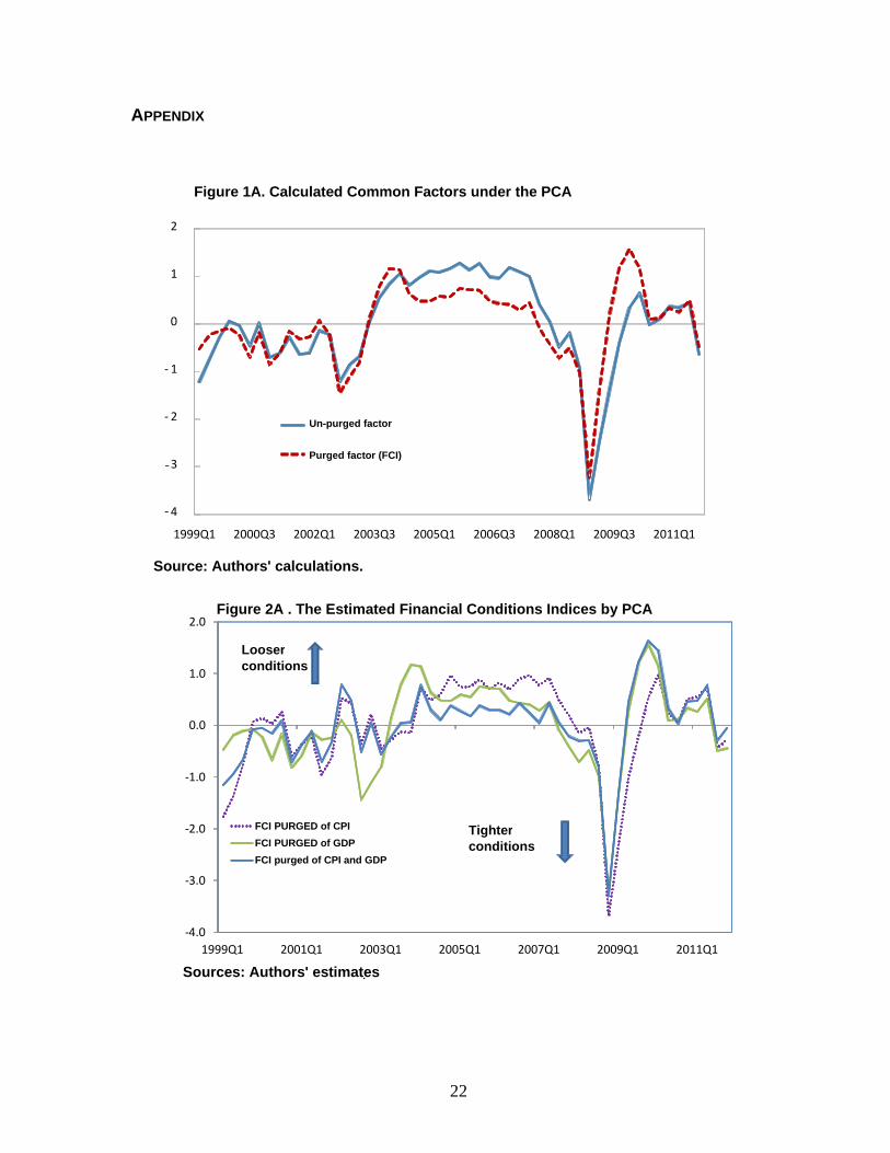
APPENDIX

- 4.0

- 3.0

- 2.0

- 1.0

0.0

1.0

2.0

1999Q1 2001Q1 2003Q1 2005Q1 2007Q1 2009Q1 2011Q1

FCI PURGED of CPI

FCI PURGED of GDP

FCI purged of CPI and GDP

Figure 2A . The Estimated Financial Conditions Indices by PCA

Sources: Authors' estimates.

Tighter conditions

Looser conditions

- 4

-3

- 2

- 1

0

1

2

1999Q1 2000Q3 2002Q1 2003Q3 2005Q1 2006Q3 2008Q1 2009Q3 2011Q1

Un-purged factor

Purged factor (FCI)

Figure 1A. Calculated Common Factors under the PCA

Source: Authors' calculations.

23

23

Table 1A. Correlation Matrix

JSE ABSA NEER SOVEREIGN NCD NPLS VIX TED SP500 EMBI LOANS_ADV

JSE 1.000 0.437 0.051 -0.549 -0.312 -0.289 -0.677 -0.213 0.633 0.383 0.339

ABSA 0.437 1.000 0.356 -0.493 -0.192 -0.441 -0.591 -0.398 0.362 0.437 0.304

NEER 0.051 0.356 1.000 -0.490 -0.427 0.079 -0.315 -0.388 0.426 0.701 -0.290

SOVEREIGN -0.549 -0.493 -0.490 1.000 0.550 0.496 0.794 0.480 -0.429 -0.473 -0.399

NCD -0.312 -0.192 -0.427 0.550 1.000 0.016 0.338 0.388 -0.315 -0.345 0.141

NPLS -0.289 -0.441 0.079 0.496 0.016 1.000 0.469 -0.227 -0.103 0.099 -0.913

VIX -0.677 -0.591 -0.315 0.794 0.338 0.469 1.000 0.479 -0.625 -0.491 -0.437

TED -0.213 -0.398 -0.388 0.480 0.388 -0.227 0.479 1.000 -0.265 -0.397 0.285

SP500 0.633 0.362 0.426 -0.429 -0.315 -0.103 -0.625 -0.265 1.000 0.526 0.020

EMBI 0.383 0.437 0.701 -0.473 -0.345 0.099 -0.491 -0.397 0.526 1.000 -0.137

LOANS_ADV 0.339 0.304 -0.290 -0.399 0.141 -0.913 -0.437 0.285 0.020 -0.137 1.000

Table 2A. Descriptive Statistics

JSE ABSA NEER SOVEREIGN NCD NPLS VIXL TED SP500 EMBI LOANS_ADV

Mean 0.23 0.27 0.12 0.22 0.07 4.21 0.08 0.00 -0.01 -0.01 0.07

Median 2.36 0.56 -0.35 -31.12 -0.01 4.85 -0.47 -0.14 5.67 -0.50 -1.18

Maximum 50.48 26.07 34.12 337.38 5.69 6.09 36.32 1.89 35.61 24.66 15.19

Minimum -47.54 -17.58 -26.33 -151.62 -3.60 1.99 -11.39 -0.38 -43.04 -26.56 -13.11

Std. Dev. 22.77 10.54 14.82 115.27 2.44 1.39 8.55 0.44 18.22 10.71 7.88

Skewness -0.36 0.57 0.36 0.73 0.27 -0.31 1.69 2.06 -0.59 -0.12 0.36

Kurtosis 2.64 3.03 2.59 2.98 2.14 1.48 8.00 8.07 2.69 3.36 2.15

Observations 52 52 52 52 52 52 52 52 52 52 52

24

24

Figure 3A. Financial Conditions Indicators*

*SP500, EMBI, ABSA, NEER, LOANS_ADV, and JSE are presented on y-o-y basis, while others are shown at their levels. All variable are demeaned.

-60

-40

-20

0

20

40

60

99 00 01 02 03 04 05 06 07 08 09 10 11

JSE (yoy change)

-20

-10

0

10

20

30

99 00 01 02 03 04 05 06 07 08 09 10 11

ABSA (yoy change)

-40

-20

0

20

40

99 00 01 02 03 04 05 06 07 08 09 10 11

NEER (yoy change)

-200

-100

0

100

200

300

400

99 00 01 02 03 04 05 06 07 08 09 10 11

SOVEREIGN

-4

-2

0

2

4

6

99 00 01 02 03 04 05 06 07 08 09 10 11

NCD

1

2

3

4

5

6

7

99 00 01 02 03 04 05 06 07 08 09 10 11

NPLS

-20

-10

0

10

20

30

40

99 00 01 02 03 04 05 06 07 08 09 10 11

VIX

-0.5

0.0

0.5

1.0

1.5

2.0

99 00 01 02 03 04 05 06 07 08 09 10 11

TED

-60

-40

-20

0

20

40

99 00 01 02 03 04 05 06 07 08 09 10 11

SP500 (yoy)

-30

-20

-10

0

10

20

30

99 00 01 02 03 04 05 06 07 08 09 10 11

EMBI

-20

-10

0

10

20

99 00 01 02 03 04 05 06 07 08 09 10 11

LOANS_ADV (yoy)