Embed Size (px)
DESCRIPTION
A Faster Approximation Scheme for Timing Driven Minimum Cost Layer Assignment. Shiyan Hu *, Zhuo Li**, and Charles J. Alpert** *Dept of ECE, Michigan Technological University **IBM Austin Research Lab. Outline. 4 X. 2 X. 1 X. Layer Assignment. - PowerPoint PPT Presentation
Citation preview
A Faster Approximation Scheme for Timing Driven Minimum Cost Layer
Assignment
A Faster Approximation Scheme for Timing Driven Minimum Cost Layer
Assignment
Shiyan Hu*, Zhuo Li**, and Charles J. Alpert**Shiyan Hu*, Zhuo Li**, and Charles J. Alpert**
*Dept of ECE, Michigan Technological University*Dept of ECE, Michigan Technological University
**IBM Austin Research Lab**IBM Austin Research Lab

2
OutlineOutline
3
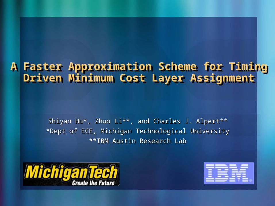
Layer AssignmentLayer Assignment
11XX
22XX
44XX
In 45nm technology, layer assignment is In 45nm technology, layer assignment is critical for timing and buffer area optimizationcritical for timing and buffer area optimization
4
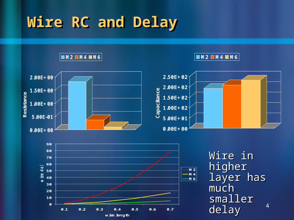
Wire RC and DelayWire RC and Delay
0
10
20
30
40
50
60
70
80
90
0.1 0.2 0.3 0.4 0.5 0.6 0.7
wire length
wir
e d
ela
y
M2M4M6
Wire in Wire in higher layer higher layer has much has much smaller delaysmaller delay
0.00E+00
5.00E-01
1.00E+00
1.50E+00
2.00E+00
Res
ista
nce
M2 M4 M6
0.00E+00
5.00E+01
1.00E+02
1.50E+02
2.00E+02
2.50E+02
Cap
acit
ance
M2 M4 M6
5
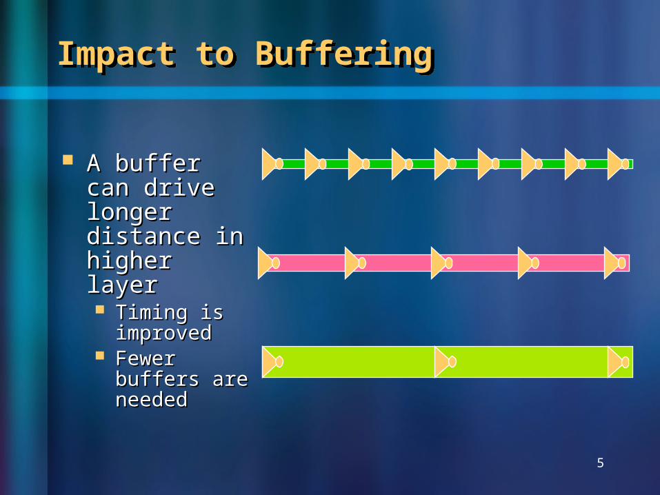
Impact to BufferingImpact to Buffering
A buffer can A buffer can drive longer drive longer distance in distance in higher layer higher layer Timing is Timing is
improvedimproved Fewer buffers Fewer buffers
are neededare needed
6
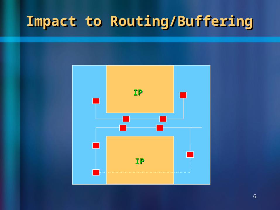
Impact to Routing/BufferingImpact to Routing/Buffering
IPIP
IPIP
7
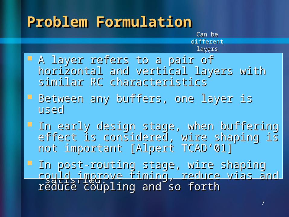
Problem FormulationProblem Formulation
Find a Find a minimal costminimal cost layer assignment such layer assignment such that the timing constraint is satisfied.that the timing constraint is satisfied.
Same LayerSame Layer
Can be Can be different layersdifferent layers
GivenGiven– A buffered Steiner A buffered Steiner
tree with n wire tree with n wire segmentssegments
– Timing constraintTiming constraint– m wire layers with m wire layers with
RC parameters and RC parameters and costcost
A layer refers to a pair of horizontal and A layer refers to a pair of horizontal and vertical layers with similar RC vertical layers with similar RC characteristicscharacteristics
Between any buffers, one layer is usedBetween any buffers, one layer is used In early design stage, when buffering effect In early design stage, when buffering effect
is considered, wire shaping is not important is considered, wire shaping is not important [Alpert TCAD’01][Alpert TCAD’01]
In post-routing stage, wire shaping could In post-routing stage, wire shaping could improve timing, reduce vias and reduce improve timing, reduce vias and reduce coupling and so forthcoupling and so forth
Fully Polynomial Time Fully Polynomial Time Approximation Scheme Approximation Scheme (FPTAS)(FPTAS)
Fully Polynomial Time Fully Polynomial Time Approximation Scheme Approximation Scheme (FPTAS)(FPTAS)
8
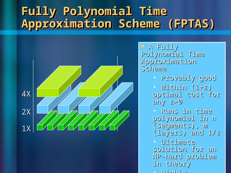
A Fully Polynomial A Fully Polynomial Time Approximation Time Approximation SchemeScheme
• Provably goodProvably good• Within (1+ɛ) Within (1+ɛ) optimal cost for optimal cost for any ɛ>0any ɛ>0• Runs in time Runs in time polynomial in n polynomial in n (segments), m (segments), m (layers) and 1/ɛ(layers) and 1/ɛ• Ultimate solution Ultimate solution for an NP-hard for an NP-hard problem in theoryproblem in theory• Highly practicalHighly practical
11XX
22XX
44XX
Previous Work in ICCAD’08Previous Work in ICCAD’08
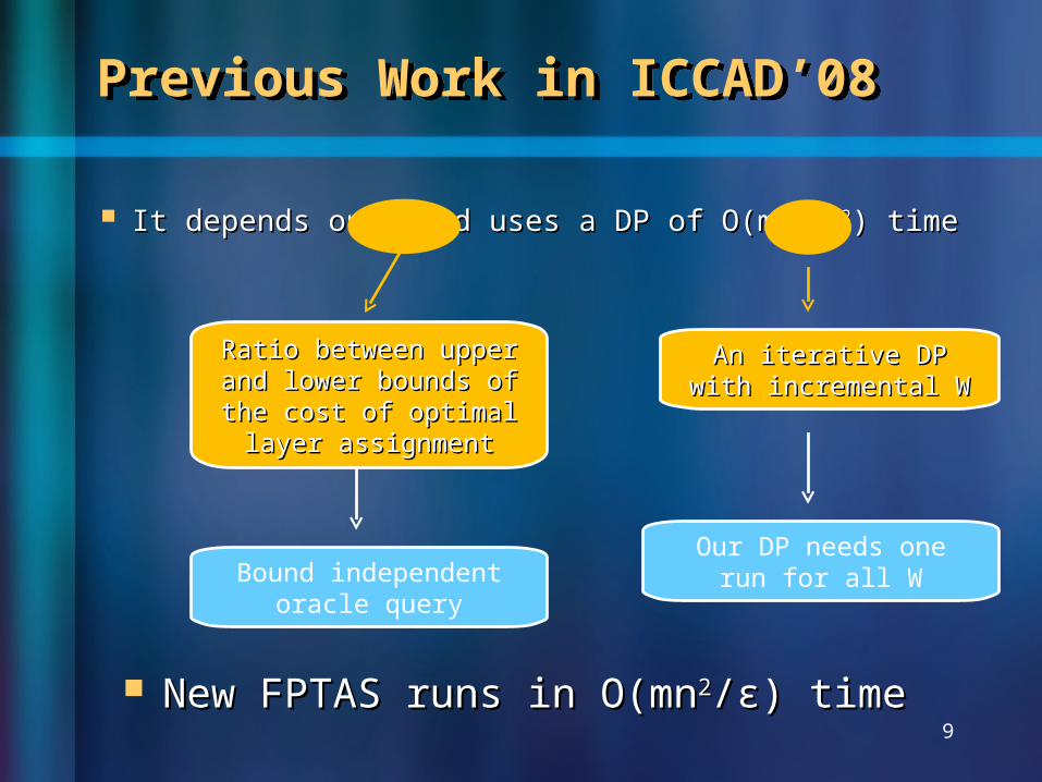
It depends on M and uses a DP of O(mnIt depends on M and uses a DP of O(mn33//ɛɛ22) time) time
9
Bound independent oracle query
Our DP needs one run for all W
New FPTAS runs in O(mnNew FPTAS runs in O(mn22//ɛɛ) time) time
Ratio between upper Ratio between upper and lower bounds of and lower bounds of the cost of optimal the cost of optimal layer assignmentlayer assignment
An iterative DP with An iterative DP with incremental Wincremental W
1010
The Rough PictureThe Rough Picture
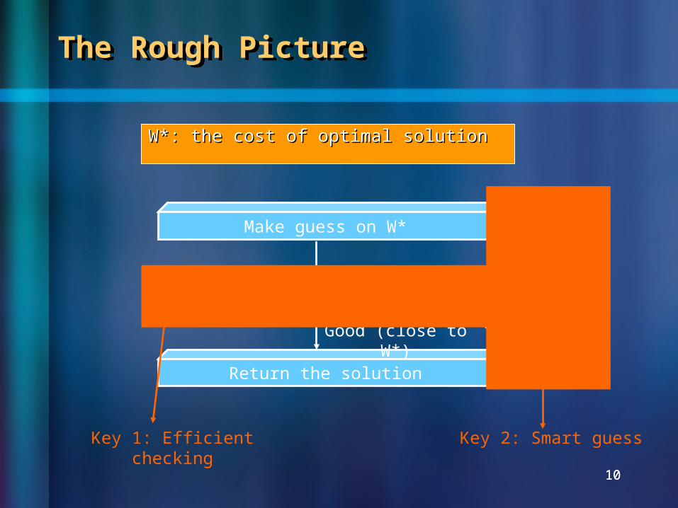
W*: the cost of optimal solutionW*: the cost of optimal solution
Check it
Make guess on W*
Return the solution
Good (close to W*)
Not Good
Key 2: Smart guessKey 1: Efficient checking
11
Key 1: Efficient CheckingKey 1: Efficient Checking
Benefit of guessBenefit of guess• Only maintain Only maintain the solutions with the solutions with cost no greater cost no greater than the guessed than the guessed costcost• Accelerate DPAccelerate DP
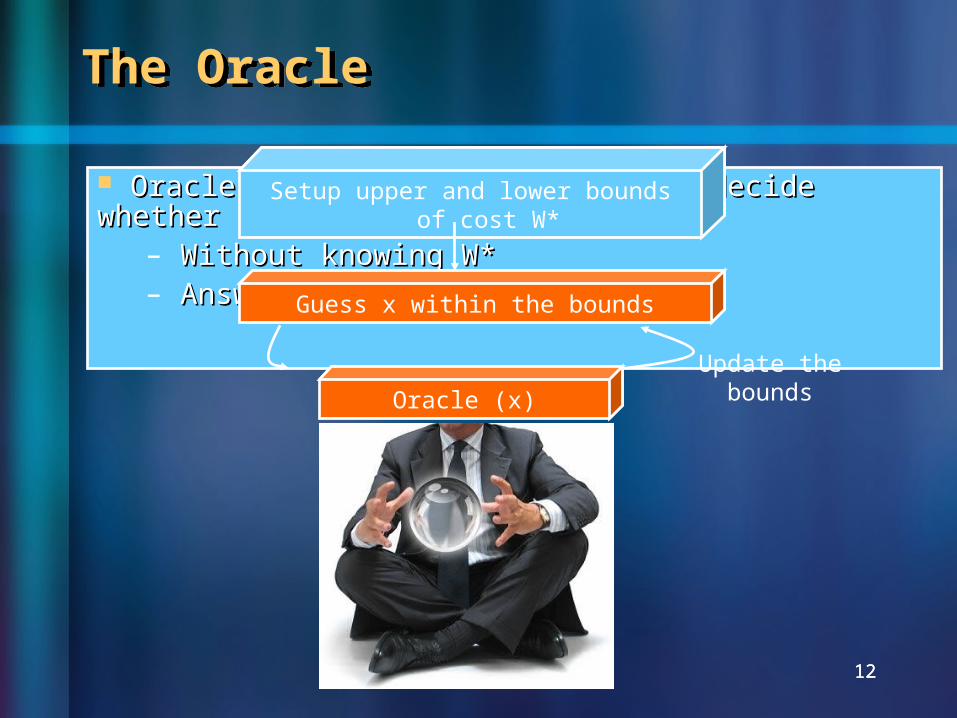
Oracle (x): the checker, able to decide whether x>W* Oracle (x): the checker, able to decide whether x>W* or notor not
– Without knowing W*Without knowing W*– Answer efficientlyAnswer efficiently
1212
The OracleThe Oracle
Oracle (x)
Guess x within the bounds
Setup upper and lower bounds of cost W*
Update the bounds

1313
Construction of Oracle(x)Construction of Oracle(x)
Scale and Scale and round each wire round each wire costcost
nx
ww
/
Only interested in Only interested in whether there is whether there is a solution with a solution with
cost up to x cost up to x satisfying timing satisfying timing
constraintconstraint
Dynamic Dynamic
ProgrammingProgramming
Perform DP to Perform DP to scaled problem scaled problem with cost bound with cost bound n/ɛ. Time n/ɛ. Time polynomial in polynomial in n/ɛn/ɛ
14
Scaling and RoundingScaling and Rounding
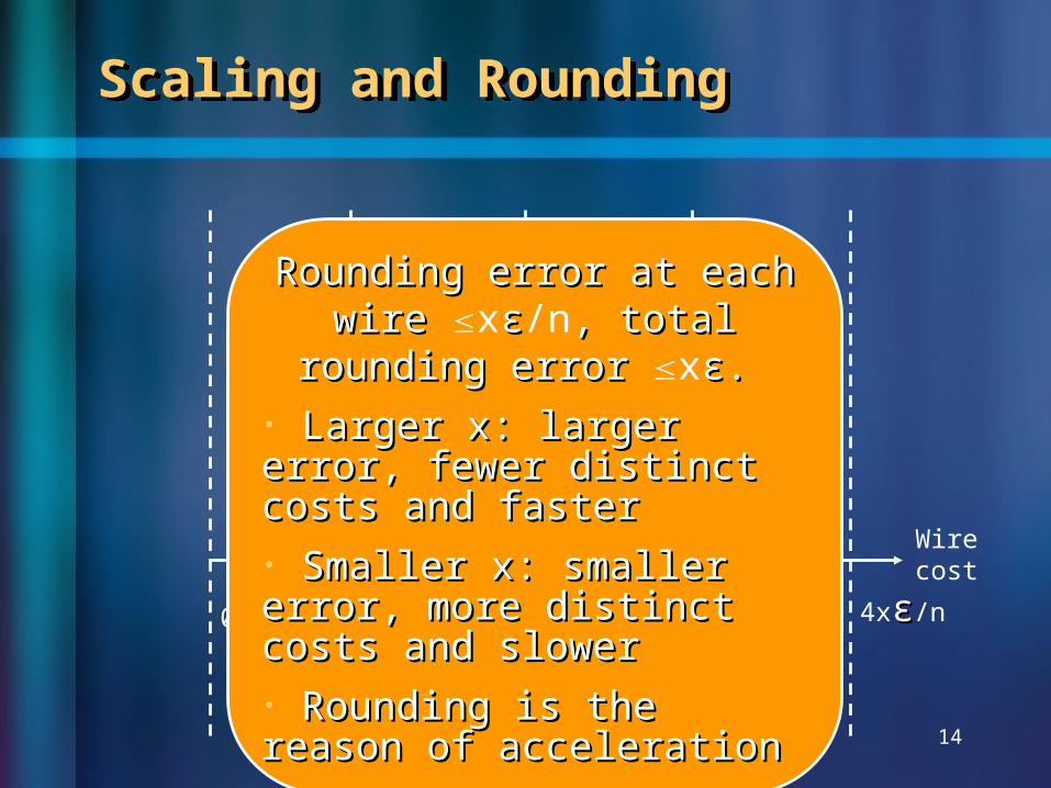
xɛɛ/n 2xɛɛ/n 3xɛɛ/n 4xɛɛ/n
Wire cost
0
Wire cost is integer after scaling and
rounding with upper bound n/ɛ. Total #
solutions is bounded in DP
Rounding error at each wire Rounding error at each wire xɛɛ/n, total rounding error , total rounding error xɛ. ɛ. • Larger x: larger error, fewer Larger x: larger error, fewer distinct costs and faster distinct costs and faster • Smaller x: smaller error, more Smaller x: smaller error, more distinct costs and slower distinct costs and slower • Rounding is the reason of Rounding is the reason of accelerationacceleration

Dynamic Programming ResultsDynamic Programming Results
15
Yes, there is a solution satisfying timing
constraint
No, no such solution
With cost rounding back, the solution has cost at most n/ɛ • xɛ/n
+ xɛ= (1+ɛ)x > W*
With cost rounding back, the solution has cost at least n/ɛ • xɛ/n
= x W*
DP result w/ all w are integers n/ɛ
16
Solution CharacterizationSolution Characterization
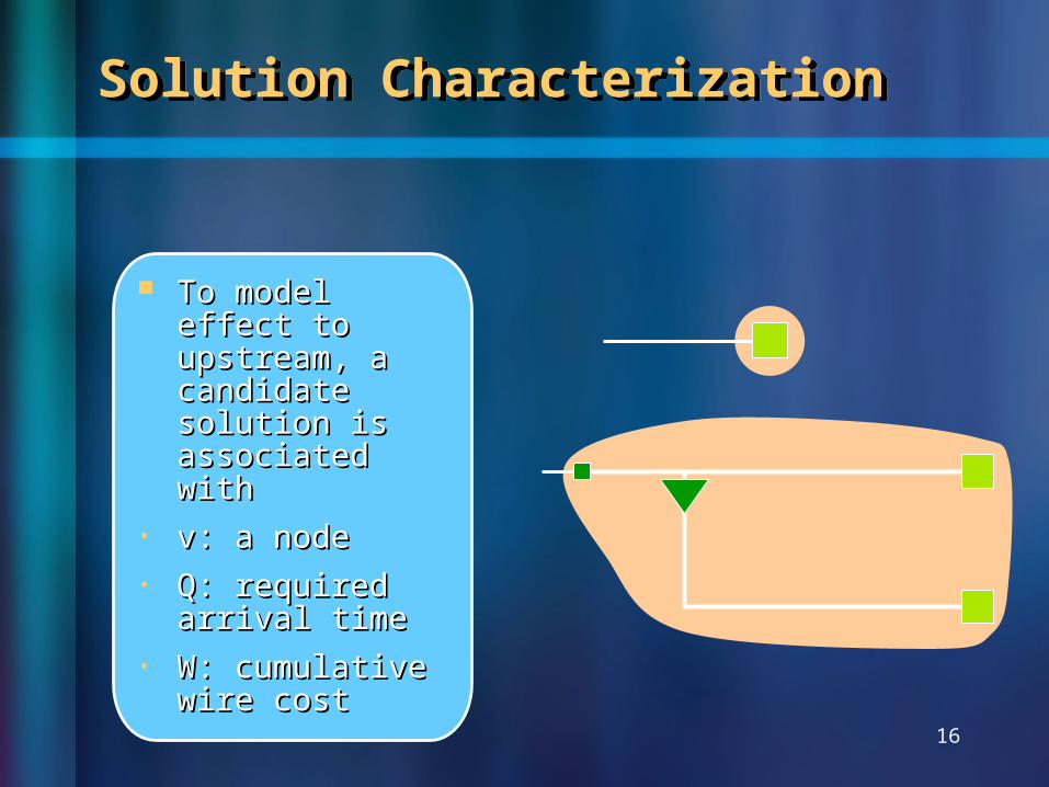
To model effect To model effect to upstream, a to upstream, a candidate candidate solution is solution is associated withassociated with
• v: a nodev: a node• Q: required Q: required
arrival timearrival time• W: cumulative W: cumulative
wire costwire cost
17
Cost (W)-Bounded Dynamic Programming (DP)Cost (W)-Bounded Dynamic Programming (DP)
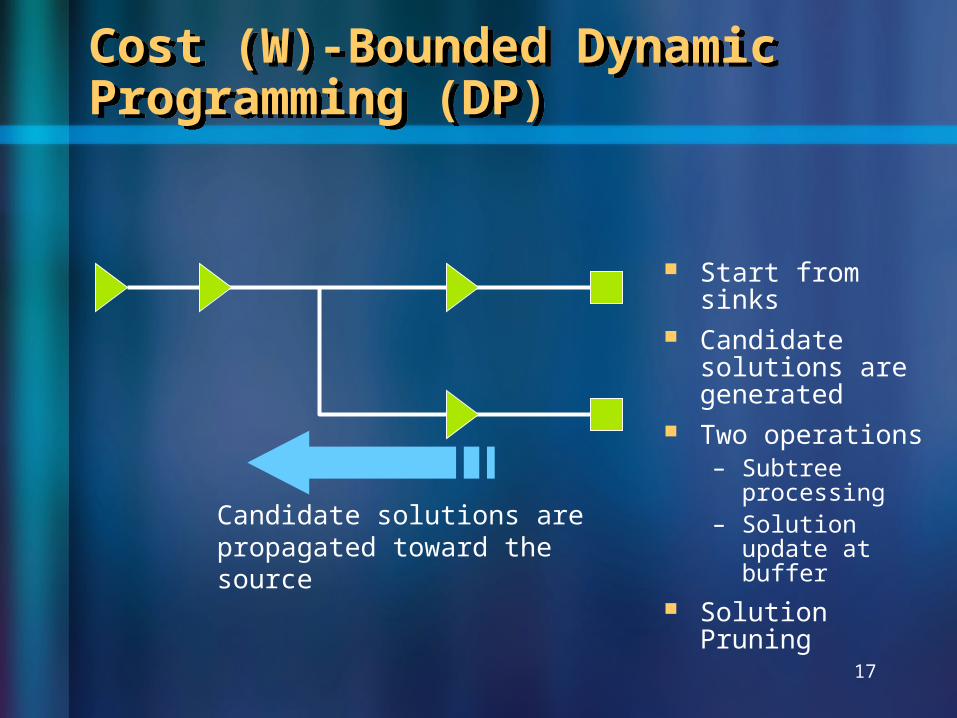
Candidate solutions are propagated toward the source
Start from sinks Candidate
solutions are generated
Two operations– Subtree
processing– Solution
update at buffer
Solution Pruning
18
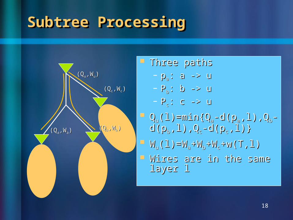
Subtree ProcessingSubtree Processing
Three pathsThree paths– ppaa: a -> u: a -> u– PPbb: b -> u: b -> u– PPcc: c -> u: c -> u
QQuu(l)=min{Q(l)=min{Qaa-d(p-d(paa,l),Q,l),Qbb--d(pd(pbb,l),Q,l),Qcc-d(p-d(pcc,l)},l)}
WWuu(l)=W(l)=Waa+W+Wbb+W+Wcc+w(T,l)+w(T,l) Wires are in the same Wires are in the same
layer llayer l
((QQuu,W,Wuu))
((QQaa,W,Waa))((QQbb,W,Wbb))
((QQcc,W,Wcc))
19
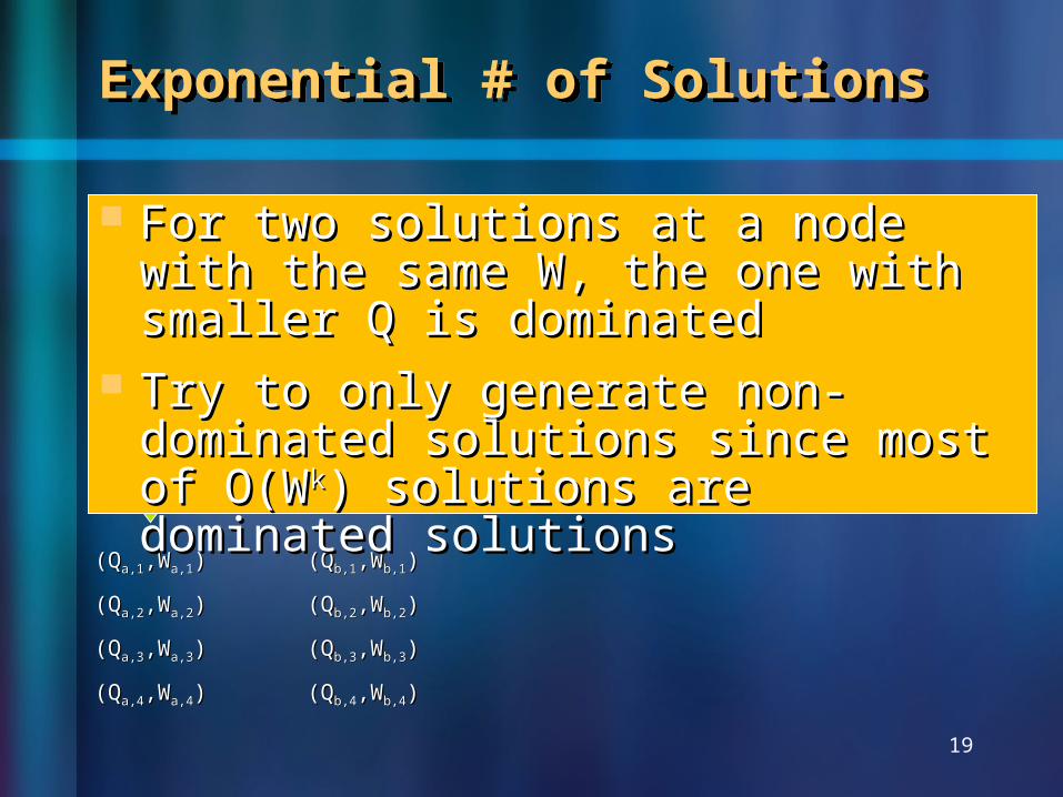
Exponential # of SolutionsExponential # of Solutions
W (=n/ɛ) solutions W (=n/ɛ) solutions at each at each downstream downstream bufferbuffer
Naïve merging Naïve merging takes O(Wtakes O(Wkk) time ) time with k brancheswith k branches
((QQa,1a,1,W,Wa,1a,1))
(Q(Qa,2a,2,W,Wa,2a,2))
(Q(Qa,3a,3,W,Wa,3a,3))
(Q(Qa,4a,4,W,Wa,4a,4))
((QQuu,W,Waa))
((QQb,1b,1,W,Wb,1b,1))
(Q(Qb,2b,2,W,Wb,2b,2))
(Q(Qb,3b,3,W,Wb,3b,3))
(Q(Qb,4b,4,W,Wb,4b,4))
((QQc,1c,1,W,Wc,1c,1))
(Q(Qc,2c,2,W,Wc,2c,2))
(Q(Qc,3c,3,W,Wc,3c,3))
(Q(Qc,4c,4,W,Wc,4c,4))
kk
For two solutions at a node with the For two solutions at a node with the same W, the one with smaller Q is same W, the one with smaller Q is dominateddominated
Try to only generate non-dominated Try to only generate non-dominated solutions since most of O(Wsolutions since most of O(Wkk) ) solutions are dominated solutionssolutions are dominated solutions
20
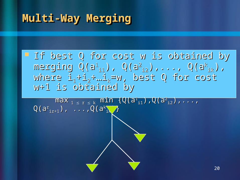
Multi-Way MergingMulti-Way Merging
If best Q for cost w is obtained by merging If best Q for cost w is obtained by merging Q(aQ(a11
i1i1), Q(a), Q(a22i2i2),..., Q(a),..., Q(akk
ikik)), where i, where i11+i+i22+…+…iikk=w, best Q for cost w+1 is obtained by=w, best Q for cost w+1 is obtained by
maxmax 1 1 r r k k min {Q(amin {Q(a11i1i1),Q(a),Q(a22
i2i2),..., Q(a),..., Q(arrir+1ir+1), ...,Q(a), ...,Q(akk
ikik)})}
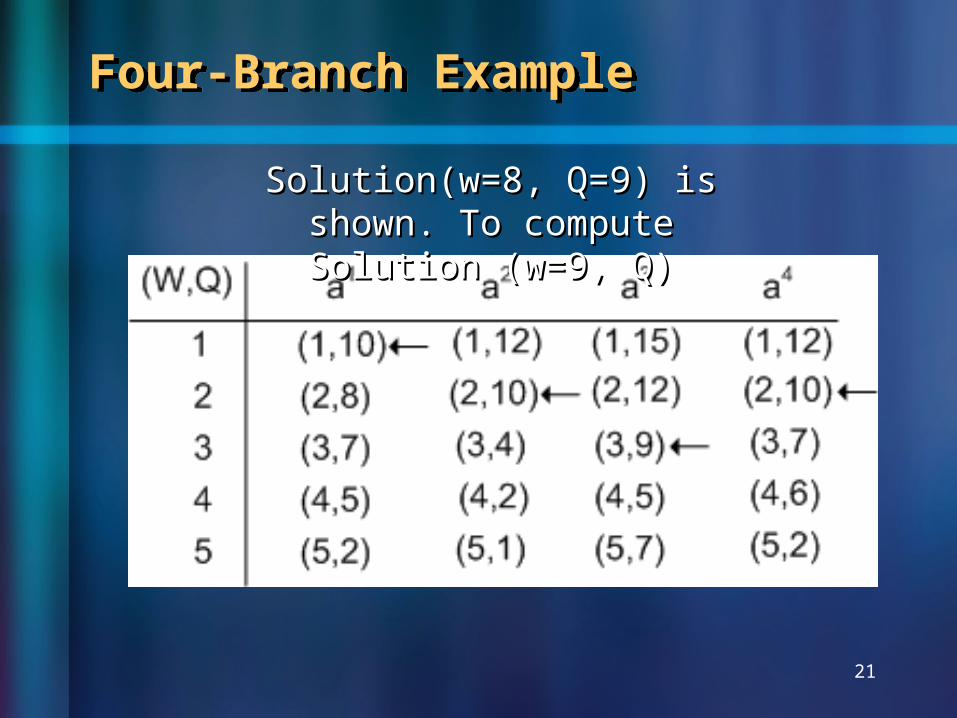
Four-Branch ExampleFour-Branch Example
21
Solution(w=8, Q=9) is Solution(w=8, Q=9) is shown. To compute Solution shown. To compute Solution
(w=9, Q)(w=9, Q)
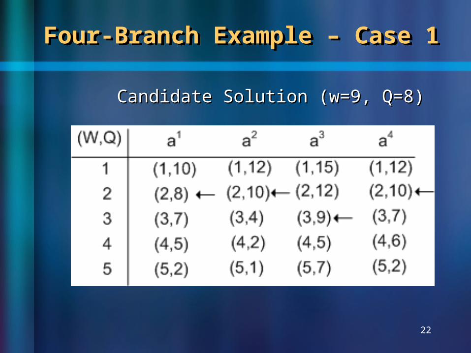
Four-Branch Example – Case 1Four-Branch Example – Case 1
22
Candidate Solution (w=9, Q=8)Candidate Solution (w=9, Q=8)
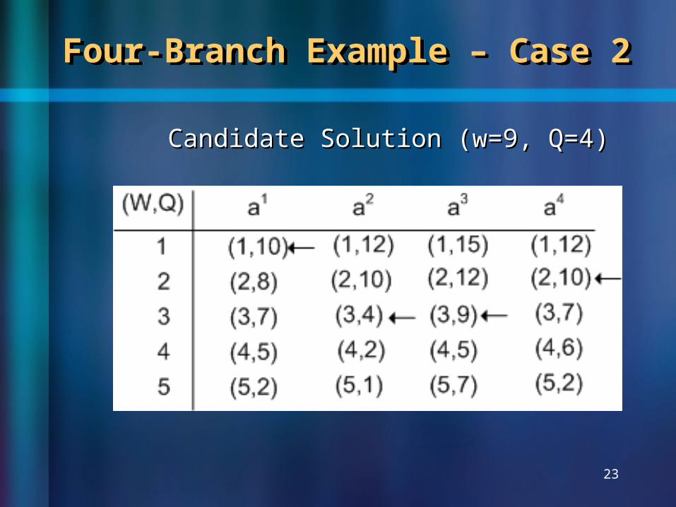
Four-Branch Example – Case 2Four-Branch Example – Case 2
23
Candidate Solution (w=9, Q=4)Candidate Solution (w=9, Q=4)

Four-Branch Example – Case 3Four-Branch Example – Case 3
24
Candidate Solution (w=9, Q=5)Candidate Solution (w=9, Q=5)
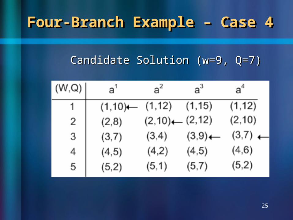
Four-Branch Example – Case 4Four-Branch Example – Case 4
25
Candidate Solution (w=9, Q=7)Candidate Solution (w=9, Q=7)
Linear Time Multi-Way MergingLinear Time Multi-Way Merging
26
Lemma: given a subtree with m layers, k Lemma: given a subtree with m layers, k branches and W non-dominated solutions at branches and W non-dominated solutions at each downstream buffer, one can merge each downstream buffer, one can merge them in O(mkW) time.them in O(mkW) time.

Solution Update at BufferSolution Update at Buffer
27
After merging, one After merging, one non-dominated non-dominated solution per layer solution per layer per cost, totally per cost, totally O(mW) solutionsO(mW) solutions
For each cost, find For each cost, find largest Q for all largest Q for all layers after buffer layers after buffer and propagate itand propagate it
((QQuu,W,Wuu))
((QQaa,W,Waa))((QQbb,W,Wbb))
((QQcc,W,Wcc))
28
Cost-Bounded DPCost-Bounded DP
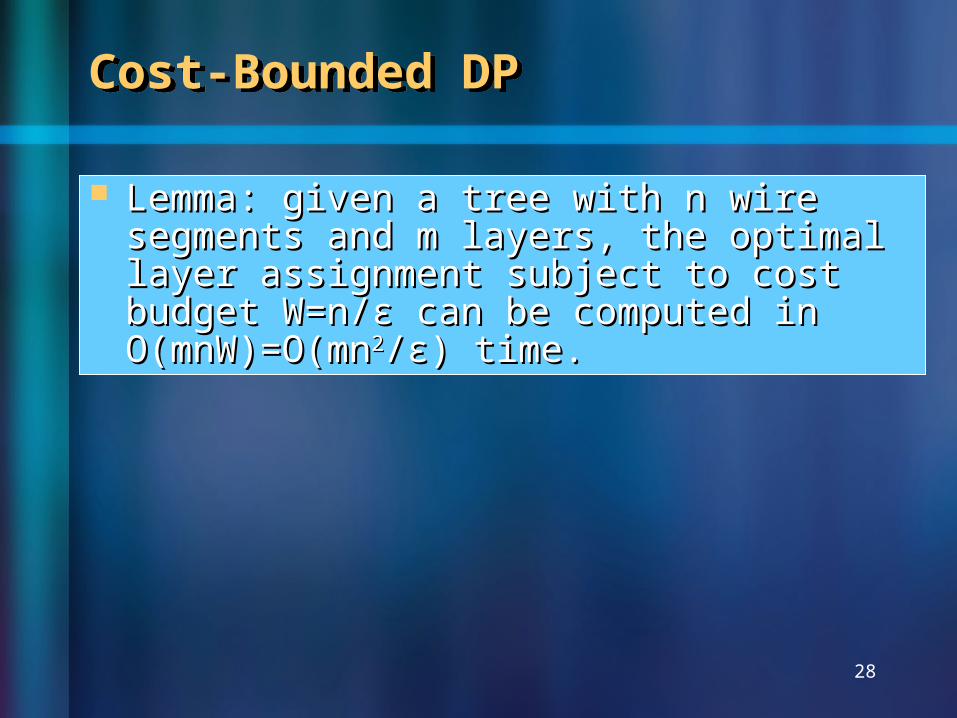
Lemma: given a tree with n wire Lemma: given a tree with n wire segments and m layers, the optimal layer segments and m layers, the optimal layer assignment subject to cost budget W=n/ɛ assignment subject to cost budget W=n/ɛ can be computed in O(mnW)=O(mncan be computed in O(mnW)=O(mn22/ɛ) /ɛ) time.time.
29
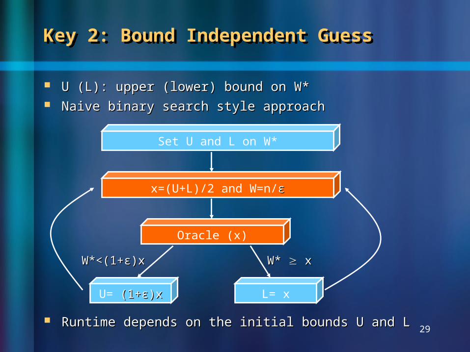
Key 2: Bound Independent GuessKey 2: Bound Independent Guess
U (L): upper (lower) bound on W*U (L): upper (lower) bound on W* Naive binary search style approachNaive binary search style approach
Runtime depends on the initial bounds U and LRuntime depends on the initial bounds U and L
Oracle (x)
x=(U+L)/2 and W=n/ɛɛ
Set U and L on W*
U= (1+ɛ)x(1+ɛ)x L= x
W*<(1+ɛ)xW*<(1+ɛ)x W* W* x x
30
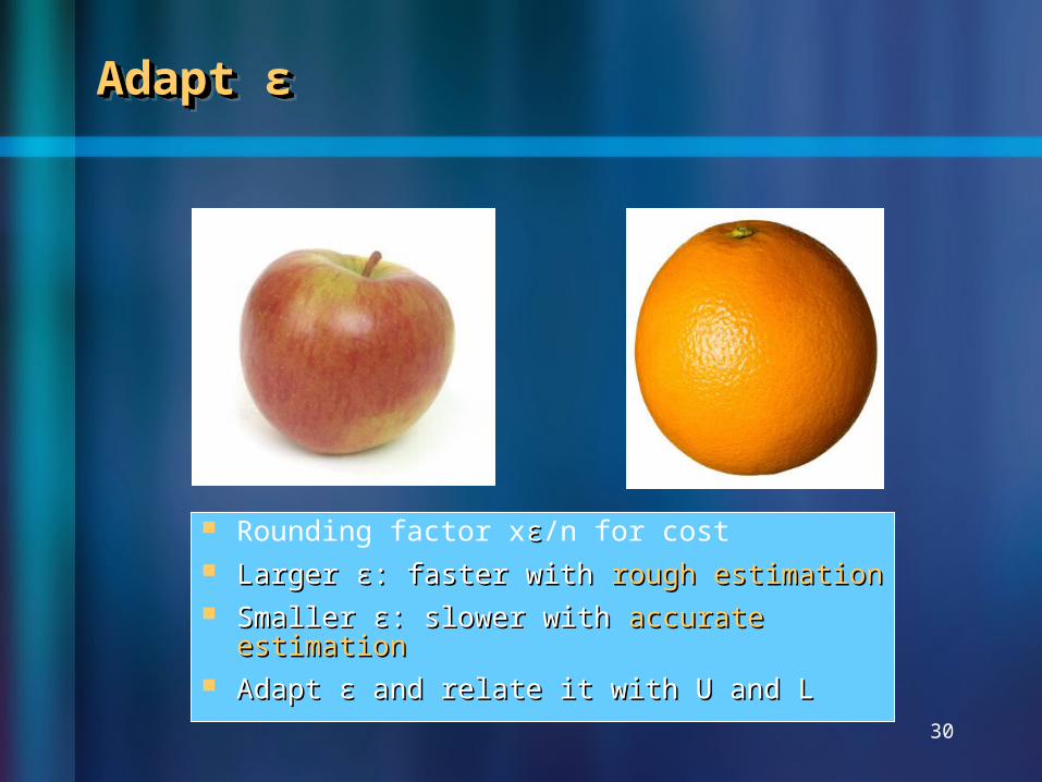
Adapt ɛAdapt ɛAdapt ɛAdapt ɛ
Rounding factor xɛɛ/n for cost Larger ɛ: faster with Larger ɛ: faster with rough estimationrough estimation Smaller ɛ: slower with Smaller ɛ: slower with accurate accurate
estimationestimation Adapt ɛ and relate it with U and LAdapt ɛ and relate it with U and L
31
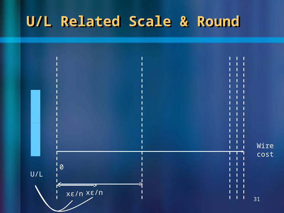
U/L Related Scale & RoundU/L Related Scale & Round
Wire cost
0U/L
xɛ/nxɛ/n
32
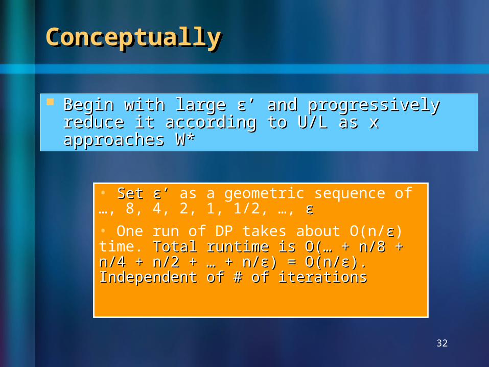
ConceptuallyConceptually
Begin with large ɛ’ and progressively reduce Begin with large ɛ’ and progressively reduce it according to U/L as x approaches W*it according to U/L as x approaches W*
• Set ɛ’Set ɛ’ as a geometric sequence of …, 8, 4, 2, 1, 1/2, …, ɛɛ
• One run of DP takes about O(n/ɛɛ) time. Total runtime is O(… + n/8 + n/4 + n/2 + Total runtime is O(… + n/8 + n/4 + n/2 + … + n/ɛ) = O(n/ɛ). Independent of # of … + n/ɛ) = O(n/ɛ). Independent of # of iterationsiterations
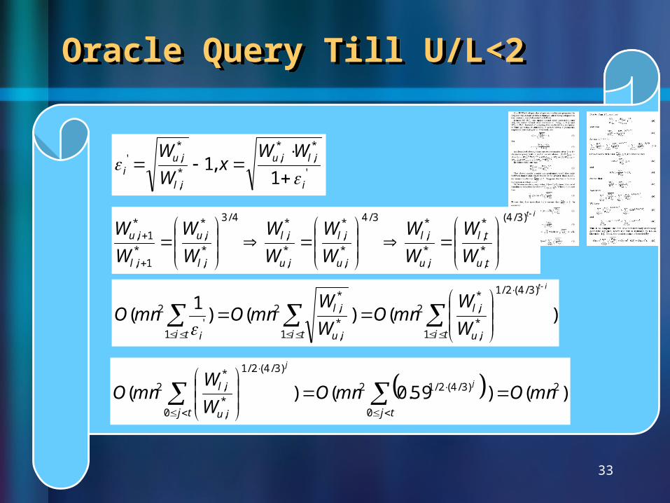
Oracle Query Till U/L<2Oracle Query Till U/L<2
33
'
*,
*,
*,
*,'
1 ,1
i
iliu
il
iui
WWx
W
W
)()()1
(
)3/4(2/1
1*,
*,2
1*,
*,2
1'
2
it
ti iu
il
ti iu
il
ti i W
WmnO
W
WmnOmnO
)() 59.0()( 2
0
)3/4(2/12
)3/4(2/1
0*,
*,2 mnOmnO
W
WmnO
tjtj iu
il j
j
it
tu
tl
iu
il
iu
il
iu
il
il
iu
il
iu
W
W
W
W
W
W
W
W
W
W
W
W
)3/4(
*,
*,
*,
*,
3/4
*,
*,
*,
*,
4/3
*,
*,
*1,
*1,
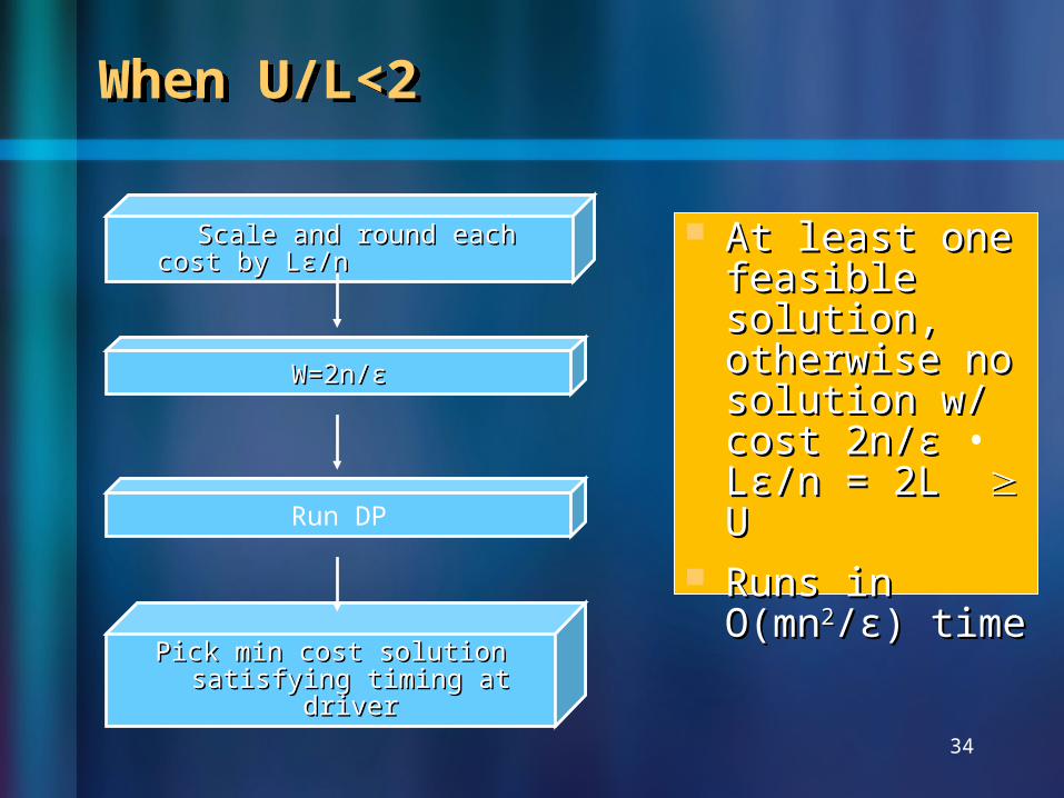
When U/L<2When U/L<2
34
At least one At least one feasible feasible solution, solution, otherwise no otherwise no solution w/ solution w/ cost 2n/ɛcost 2n/ɛ • Lɛ/n = 2L Lɛ/n = 2L U U
Runs in Runs in O(mnO(mn22/ɛ) time/ɛ) time
Pick min cost solution satisfying Pick min cost solution satisfying timing at drivertiming at driver
W=2n/ɛW=2n/ɛ
Scale and round each cost by Scale and round each cost by Lɛ/nLɛ/n
Run DP
35
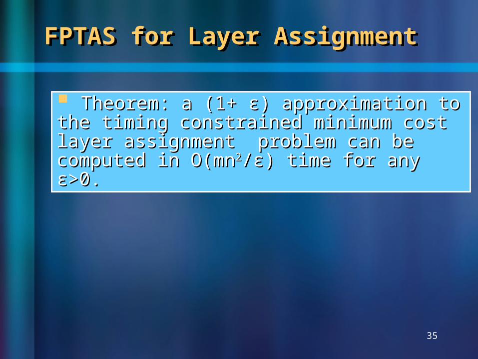
FPTAS for Layer AssignmentFPTAS for Layer Assignment
Theorem: a (1+ ɛ) approximation to the Theorem: a (1+ ɛ) approximation to the timing constrained minimum cost layer timing constrained minimum cost layer assignment problem can be computed in assignment problem can be computed in O(mnO(mn22/ɛ) time for any ɛ>0./ɛ) time for any ɛ>0.
36
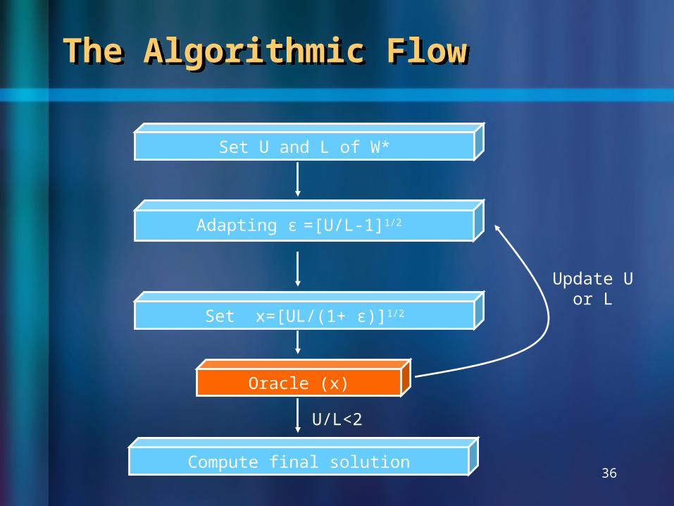
The Algorithmic FlowThe Algorithmic Flow
Oracle (x)
Adapting ɛ =[U/L-1]1/2
Set U and L of W*
Set x=[UL/(1+ ɛ)]1/2
Update U or L
U/L<2
Compute final solution
37
ExperimentsExperiments
Experimental SetupExperimental Setup– 1000 industrial nets 1000 industrial nets
Compared to Dynamic Compared to Dynamic Programming and the previous Programming and the previous FPTAS [ICCAD’08]FPTAS [ICCAD’08]
3838
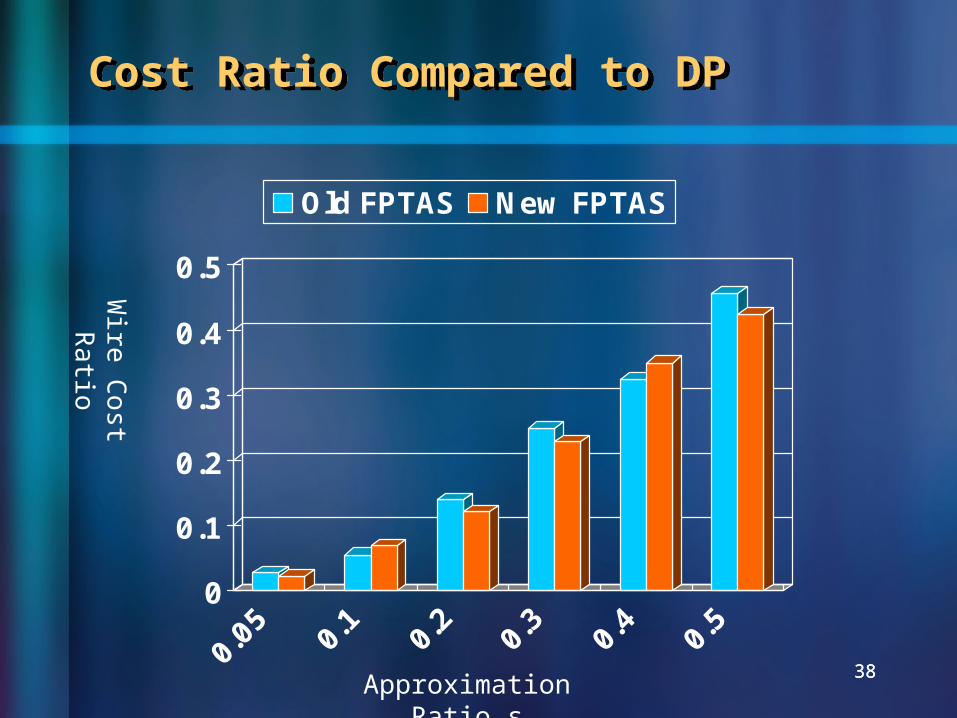
Cost Ratio Compared to DPCost Ratio Compared to DP
Approximation Ratio ɛ
Wire
Cost R
atio
0
0.1
0.2
0.3
0.4
0.5
0.05 0.
10.2
0.3
0.4
0.5
Old FPTAS New FPTAS
3939
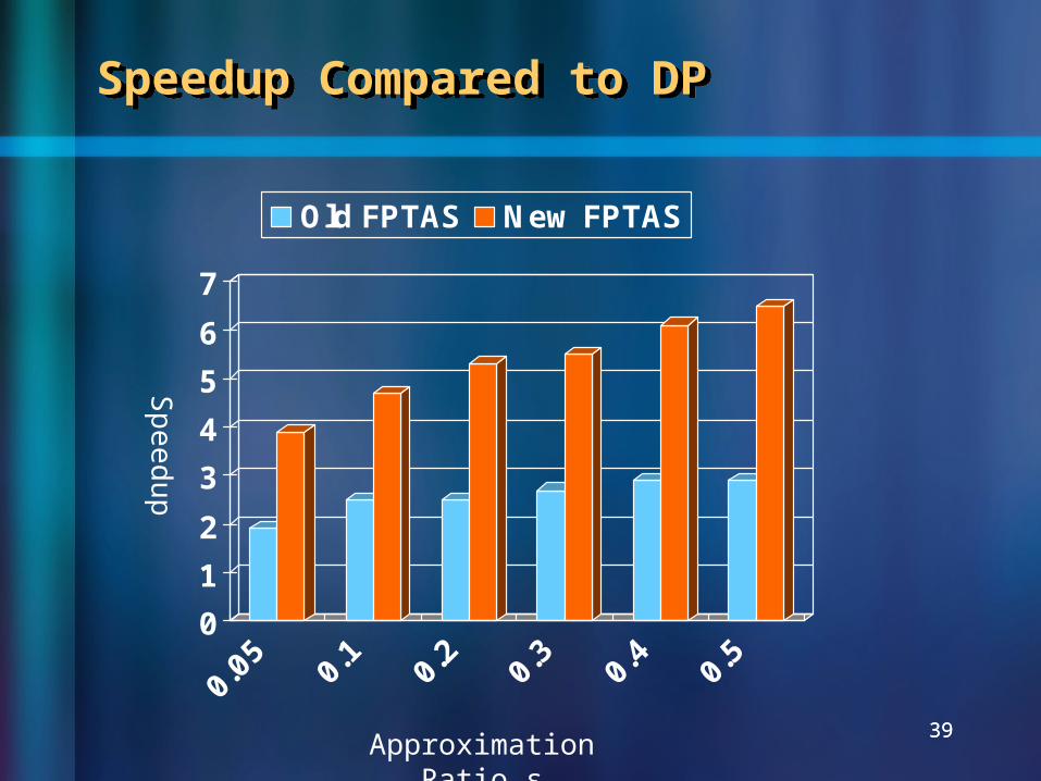
Speedup Compared to DPSpeedup Compared to DP
Approximation Ratio ɛ
Sp
eed
up
0
1
2
3
4
5
6
7
0.05 0.
10.2
0.3
0.4
0.5
Old FPTAS New FPTAS
40
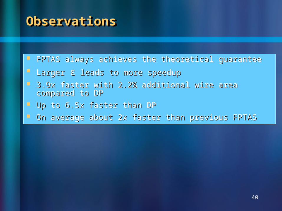
ObservationsObservations
FPTAS always achieves the theoretical guaranteeFPTAS always achieves the theoretical guarantee Larger Larger ɛɛ leads to more speedup leads to more speedup 3.9x faster with 2.2% additional wire area compared to 3.9x faster with 2.2% additional wire area compared to
DPDP Up to 6.5x faster than DPUp to 6.5x faster than DP On average about 2x faster than previous FPTASOn average about 2x faster than previous FPTAS
41
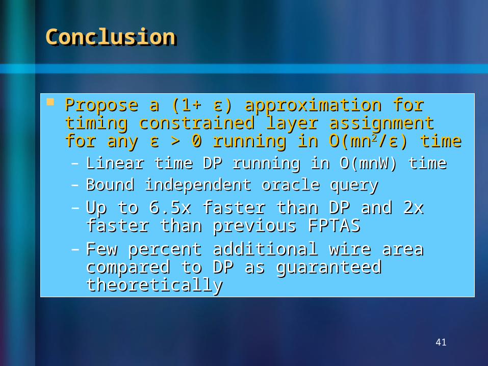
ConclusionConclusion
Propose a (1+ ɛ) approximation for timing Propose a (1+ ɛ) approximation for timing constrained layer assignment for any ɛ > 0 constrained layer assignment for any ɛ > 0 running in O(mnrunning in O(mn22/ɛ) time/ɛ) time– Linear time DP running in O(mnW) timeLinear time DP running in O(mnW) time– Bound independent oracle queryBound independent oracle query– Up to 6.5x faster than DP and 2x faster Up to 6.5x faster than DP and 2x faster
than previous FPTASthan previous FPTAS– Few percent additional wire area Few percent additional wire area
compared to DP as guaranteed compared to DP as guaranteed theoreticallytheoretically

42
Thanks


![Faster approximation algorithms for packing and covering problems · Faster approximation algorithms for packing and covering problems ... [19] to design an algorithm that computes](https://img.pdfslide.us/doc/110x75/6043da86f8286a70a40ff39b/faster-approximation-algorithms-for-packing-and-covering-faster-approximation-algorithms.jpg)