NASA/TP–2004-212283

A Fast-Time Simulation Tool for Analysis of AirportArrival Traffic

Frank Neuman, Heinz Erzberger, and Larry A. Meyn

August 2004

https://ntrs.nasa.gov/search.jsp?R=20050110290 2018-07-18T12:19:21+00:00Z

Since its founding, NASA has been dedicated to theadvancement of aeronautics and space science. TheNASA Scientific and Technical Information (STI)Program Office plays a key part in helping NASAmaintain this important role.

The NASA STI Program Office is operated byLangley Research Center, the Lead Center forNASA’s scientific and technical information. TheNASA STI Program Office provides access to theNASA STI Database, the largest collection ofaeronautical and space science STI in the world.The Program Office is also NASA’s institutionalmechanism for disseminating the results of itsresearch and development activities. These resultsare published by NASA in the NASA STI ReportSeries, which includes the following report types:

• TECHNICAL PUBLICATION. Reports ofcompleted research or a major significant phaseof research that present the results of NASAprograms and include extensive data or theoreti-cal analysis. Includes compilations of significantscientific and technical data and informationdeemed to be of continuing reference value.NASA’s counterpart of peer-reviewed formalprofessional papers but has less stringentlimitations on manuscript length and extentof graphic presentations.

• TECHNICAL MEMORANDUM. Scientific andtechnical findings that are preliminary or ofspecialized interest, e.g., quick release reports,working papers, and bibliographies that containminimal annotation. Does not contain extensiveanalysis.

• CONTRACTOR REPORT. Scientific andtechnical findings by NASA-sponsoredcontractors and grantees.

The NASA STI Program Office . . . in Profile

• CONFERENCE PUBLICATION. Collectedpapers from scientific and technical confer-ences, symposia, seminars, or other meetingssponsored or cosponsored by NASA.

• SPECIAL PUBLICATION. Scientific, technical,or historical information from NASA programs,projects, and missions, often concerned withsubjects having substantial public interest.

• TECHNICAL TRANSLATION. English-language translations of foreign scientific andtechnical material pertinent to NASA’s mission.

Specialized services that complement the STIProgram Office’s diverse offerings include creatingcustom thesauri, building customized databases,organizing and publishing research results . . . evenproviding videos.

For more information about the NASA STIProgram Office, see the following:

• Access the NASA STI Program Home Page athttp://www.sti.nasa.gov

• E-mail your question via the Internet tohelp@sti.nasa.gov

• Fax your question to the NASA Access HelpDesk at (301) 621-0134

• Telephone the NASA Access Help Desk at(301) 621-0390

• Write to:NASA Access Help DeskNASA Center for AeroSpace Information7121 Standard DriveHanover, MD 21076-1320

NASA/TP–2004-212283

A Fast-Time Simulation Tool for Analysis of AirportArrival Traffic

Frank NeumanColumbia, California

Heinz Erzberger and Larry A. MeynAmes Research Center, Moffett Field, California

August 2004

National Aeronautics andSpace Administration

Ames Research CenterMoffett Field, California 94035-1000

Available from:

NASA Center for AeroSpace Information National Technical Information Service7121 Standard Drive 5285 Port Royal RoadHanover, MD 21076-1320 Springfield, VA 22161(301) 621-0390 (703) 487-4650

iii

CONTENTS

SYMBOLS..................................................................................................................................... V

DEFINITION OF TERMS ..........................................................................................................VI

SUMMARY .................................................................................................................................... 1

INTRODUCTION.......................................................................................................................... 2

BASIC ELEMENTS OF A STOCHASTIC ARRIVAL TRAFFIC SCHEDULINGSIMULATION ............................................................................................................................... 3

Airport Simulation ....................................................................................................................... 3Modeling Traffic .......................................................................................................................... 4The Scheduler .............................................................................................................................. 7TRACON Rescheduling to Minimize ∆DOC................................................................................ 8Adapting the FTS Scheduler for Other Airports.......................................................................... 10

EARLIER STUDIES USING FAST-TIME SIMULATION ...................................................... 10

PROPOSED NEW USE OF FTS................................................................................................. 11Present Arrival Time Distribution at Hub Airport ....................................................................... 12Ground Delay Program Insights for Normal Traffic.................................................................... 12

RESULTS FOR EXAMPLE PROBLEM ................................................................................... 13Scheduled Delays With and Without Slot Assignment................................................................ 13Interaction Between Center and TRACON Scheduling............................................................... 16

CONCLUDING REMARKS ....................................................................................................... 22

REFERENCES............................................................................................................................. 23

FIGURES ..................................................................................................................................... 25

iv

v

SYMBOLS

AAR airport acceptance rate (set by TRACON)

ata actual time of arrival at runway

ataFH actual time of arrival at the freeze horizon

ATC air-traffic control

CDM collaborative decision-making

CTAS Center TRACON Automation System

DDF Delay Distribution Function ( Function that distributes delays between Center andTRACON)

DFW Dallas/Ft. Worth airport

∆DOC direct operating cost (additional cost due to TMA commanded delays in the Centerand TRACON)

dTmax portion of the total delay computed in the Center that is completely assigned to theTRACON; the remainder assigned to the Center

etaFH estimated time of arrival at a feeder fix

etaj estimated arrival time at the jth runway, given no interfering traffic, j = 0-2 (3runways)

eta3 minimum time of arrival (given no interfering traffic)

FAST Final Approach Spacing Tool (a decision-support tool for terminal area controllers)

FCFS first-come, first-served scheduling

fferrD delay due to feeder fix arrival errors

fhD delay due to freeze horizon arrival errors

FTS fast-time simulation

GDP ground-delay program

NE northeast feeder fix to the DFW airport

vi

NW northwest feeder fix to the DFW airport

RBS ration-by-schedule

SE southeast feeder fix to the DFW airport

STA scheduled time of arrival (a parameter used in TMA)

SW southwest feeder fix to the DFW airport

TMA Traffic Management Advisor (a decision-support tool for Center controllers)

TRACON Terminal Radar Approach Control

DEFINITION OF TERMS

Airline schedule: Gate-to-gate departure and arrival times assigned by the airlines.

Connectivity: A cost factor which has been mentioned in this report, but could not be computedbecause of limited information publicly available. One hundred percent connectivity means that allpassengers who need to transfer have sufficient time to do so. This can be achieved, at a cost, byscheduling long times at the gates.

Freeze-horizon: Distance (or in 1996 time) to feeder fix where scheduled feeder-fix arrival times arefrozen.

Normal traffic: Traffic not restricted by unusual conditions. Traffic that attempts to meet airlineschedules; especially in hub airports it has many sharp traffic peaks.

Squared traffic: Around each traffic peak, it is proposed that the airlines assign new scheduled timesof arrival at the freeze horizons (slots) spaced at equal intervals. By including some of the originallow-density traffic skirts around the traffic peak, each new scheduled traffic peak is made into arectangle.

Stream class: Separate routes for jets and other aircraft up to a merge point.

TMA schedule: If too many aircraft are scheduled by the airlines to arrive in a short interval of time,or if random arrival errors at the freeze horizon cause an airport to become overloaded, TMA delaysaircraft to meet en-route and landing safety restrictions.

TRACON schedule: In the TRACON, aircraft are rescheduled by FAST including updated runwayassignments as functions of actual feeder-fix arrival times.

1

A FAST-TIME SIMULATION TOOL FOR ANALYSIS OF AIRPORTARRIVAL TRAFFIC

Frank Neuman,* Heinz Erzberger, and Larry A. Meyn

Ames Research Center

SUMMARY

The basic objective of arrival sequencing and scheduling in air-traffic control automation is to matchtraffic demand and airport capacity while minimizing delays. The principle underlying practicalsequencing and scheduling algorithms currently in use is referred to as first-come-first-served(FCFS). One of the tools developed by NASA is the Traffic Management Advisor (TMA), which theFAA has deployed at several hub airports. TMA is an element of the Center TRACON AutomationSystem (CTAS), a suite of decision-support tools developed by NASA for controllers. Prior todeployment, the TMA scheduling software had to be tested in a real-time simulation, which wasvery manpower and time intensive; as a result, only relatively few traffic situations could besimulated. In order to estimate the statistical performance of the system we have written a fast-timesimulation of the scheduling process built into TMA, which preserves TMA’s important features,but does not involve human interaction, and which can perform many simulations in a short time. Touse this simulation, we model the specific airport, the traffic, and especially the deviations fromestimated arrival times. These times are measured at distances where Center controllers begin toregulate the traffic (freeze horizons), and at points close to the airport (feeder fixes) where TRACONcontrollers take over. This report reviews the development of the simulation and several earlierstudies of scheduling algorithms that were evaluated using this simulation. In order to demonstrateanother use of this method of fast-time simulation, we examine the effect on arrival delays ofminimally altering arrival traffic schedules at a hub airport. It is assumed that the original airlinearrival schedule for a hub airport with its multiple peaks is optimal from the airline standpoint.Without upsetting the multiple peak structure, it is proposed to reduce delays by using equallyspaced slot assignments around each traffic peak. This preserves each traffic peak but spreads it outsufficiently to substantially reduce air-traffic management enforced delays. Fast-time simulation isused to evaluate the method in the presence of errors. Results show that this method can indeedachieve substantially reduced delays and improved arrival order.

*Aerospace Engineer, retired from NASA Ames Research Center.

2

INTRODUCTION

The continued growth of air traffic within the United States has led to increased congestion anddelays in the terminal airspace surrounding the Nation’s busier airports. The problem is exacerbatedat hub airports, where air carriers schedule large numbers of flights to arrive and depart within shorttime periods, resulting in multiple traffic peaks during the day. To air carriers, hubbing makes goodeconomic and competitive sense. At the same time, however, hubbing operations lead to manyovercapacity traffic peaks, which precipitate delays that can directly affect the economic efficiencyof an air carrier’s flight operations. To ensure that the safe capacity of the terminal area is notexceeded, air-traffic management (ATM) often places restrictions on arrival flights that aretransitioning from en route to terminal airspace. The constraint of arrival traffic is commonlyreferred to as arrival flow management.

Air-traffic management automation tools used in arrival flow management are primarily based onthe first-come-first-served (FCFS) principle. One of the tools designed by NASA is the trafficmanagement advisor (TMA), which is now used by the FAA at several hub airports. Aircraft arescheduled so that they arrive in first-come-first-served order based on an estimated time of arrival atthe runway (ETA) at about 200 miles from touchdown (the freeze horizon). For moderate trafficdensities, and no unusual weather conditions, FCFS orders the arrivals approximately in the orderdesired by the airlines. When, however, too many aircraft are scheduled by the airlines to arrive in ashort interval of time, it is necessary for TMA to delay aircraft in both Center and TRACONairspace, and this process can change the TMA scheduled landing order substantially from theairline-desired order.

As part of its collaborative arrival planning research and development program, NASA is exploringwhat airlines and the FAA can do jointly to reduce the arrival delays that presently occur in hubairport traffic. The ground delay program (GDP) will be used as a model for the various aspects ofaccomplishing the task, without affecting traffic connectivity. Decreased connectivity is a cost item,which only airlines can compute by knowing, at least statistically, passenger destinations. The airlinemust estimate both the probability that a passenger misses his connection and the cost of his missingit. One important question is: How much can the airlines change schedules to avoid the sharp trafficpeaks in the daily traffic in order to reduce delays without passengers missing their connections? Wedo not have connectivity data with which to study this question in detail. Hence we have chosen anexample for traffic improvement, which only slightly changes the arrival times, and which thereforeshould not affect connectivity.

Since real-time simulations and field tests are expensive to conduct and slow to produce statisticalresults, fast-time simulation is used for this initial study.

3

BASIC ELEMENTS OF A STOCHASTIC ARRIVAL TRAFFIC SCHEDULINGSIMULATION

We will first deal with a specific fast-time simulation, that of the Noon Balloon traffic peak in 1996at Dallas Fort Worth Airport. The simulation models the runways, the traffic, and the scheduler usedin TMA. Next, we will discuss how this simulation may be adapted to study traffic at differentairports and in different traffic situations. A diagram of the overall process and its components isshown in figure 1.

Airport Simulation

The traffic situation is modeled for an airport with four feeder fixes and three independent runwaysavailable for landings. For this example the most common configuration used at DFW in 1996 waschosen: runways 18, 17, and 13. Since 1996, DFW has added a fourth runway, which has somewhatalleviated the delays during rush periods such as the Noon Balloon. In spite of this, AmericanAirlines plans to reduce the peak magnitudes and double the number of the peaks. However, thethree-runway configuration at DFW remains important because of its use during certain adverseweather conditions. The three-runway case was modeled according to the landing practices thatexisted in 1996 (fig. 2(a)). Jets and turboprops arrive at each of the four feeder fixes in twoindependent streams (fig. 2(b)); the figure shows the traffic during the Noon Balloon time interval.The assumption of two streams per feeder fix is necessary in order to simulate the in-trail constraintsin the Center. Inside TRACON, aircraft have different flight times and routes that depend on thespecific entry feeder fix and landing runway threshold. Such flight times can only be achieved ifcontrollers have to deal with few aircraft, which happens between traffic peaks. The preferredrunway is modeled as the runway with a minimum flight time from the feeder fix.

The times given in table 1 for north flow and south flow of the traffic are the minimum times fromfeeder fix to runway threshold. The blank spots in the table are for flightpaths that are usually neverchosen, and therefore no times are given. The data were taken from calculations performed by theTMA used in the field trial in 1996; the calculations were verified by flight data. It should be notedthat, in the actual system, these times are calculated in real time to account for winds.

In the specific simulation considered here, the total delay between Center and TRACON wasseparated because we are interested in determining the interactions of airport arrival rate (AAR) anddelay distribution function (DDF). This is accomplished by a delay distribution with a parameterdTmax and will be discussed briefly in the next section.

Depending on the type of investigation, either a synthetic airport or an existing airport may besimulated. Runways can also be removed from the model of an existing airport by setting the feeder-fix-to-runway-threshold times of the deactivated runways to large values. This will result in thescheduler avoiding those runways. Runways can also be added by adding another line to the matrixin table 1, where all values are likely to change somewhat. This would be done, for instance, if theintention was to simulate DFW with the fourth runway installed.

4

Table 1. Minimum feeder fix to runway threshold times for three runways, sec

North flow South flow

NW NE SW SE NW NE SW SE a/c type

36L 649 723 592 — 13R 590 — — 950

35C 716 730 610 626 18R 665 730 860 960 Jets

31R 820 645 — 621 17L 770 635 920 980

36L 715 812 587 — 13R 650 — 820 — Large

35C 804 — 608 650 18R 720 820 890 1050 Turbo-

31R — 723 — 625 17L 850 710 790 900 props

When a traffic management system is to be newly installed at an airport, it is best to get data similarto those shown in table 1 from radar data taken during intervals of low traffic density. Flightpathsfrom each feeder fix to each possible runway threshold are established based on air-traffic controllerexperience. The choice of these paths and their minimum and maximum flight times are a matter ofexperience.

Modeling Traffic

For this simulation, 1996 traffic is used, since detailed field test data are available. The density of thetraffic at DFW has repeatable peaks, with periods of light traffic between peaks. The traffic peak,which we examined in detail, is the “Noon Balloon” at DFW, which was the time interval of themost prominent traffic peak at DFW. To get realistic answers, data were collected for six separatedays in 1996 during which we were doing field tests: Thursday, 18 April; Friday, 26 April; Monday,29 April; Tuesday, 30 April; Friday, 14 June; and Wednesday, 17 July. From the complete data setwe abstracted the aircraft identification (ID), aircraft type (to derive the classification: heavy jet,large jet, or large turbo prop), feeder fix crossed, and time the aircraft crossed the TMA freezethreshold. Not all scheduled aircraft showed up on all days. We included, nevertheless, all otheraircraft in each simulated Noon Balloon, except those aircraft with IDs showing up on a single dayonly. For this analysis, the lighter traffic that surrounds the Noon Balloon was also included. Theseparations between one traffic peak and the next were sufficiently long so that all TMA scheduleddelays due to one rush could be reduced before the next rush began, and each rush could therefore beindependently modeled. For the purpose of this simulation, nominal arrival times at the freezehorizons were chosen as the average of the arrival times of the aircraft with the same ID.

For statistical fast-time analysis the arrival time error distributions at the freeze horizons are alsoneeded. Since, in current operations, no attempt is made by the airlines to control these times, thesevariations are not related to the aircraft’s capability to meet these times, but they are important in

5

that they influence gate arrival times. The freeze-horizon arrival variations depend on a variety ofrandom factors. As a reasonable model of these errors, bell-shaped error probability distributionswith a range of ±200 or ±400 sec were chosen for all aircraft. Adding three properly scaledrectangular pseudorandom variables generated the distributions. Fortunately, as will be shown, theaverage total delays over all aircraft are relatively insensitive with respect to the magnitude of thearrival time errors.

In simulating traffic, one can use either synthetic or actual traffic. When simulating synthetic trafficwe have complete freedom in selecting the aircraft mix, the traffic rushes from any direction, and thetraffic density. This is useful when one wants to test the traffic management system for a number ofconditions. Our early investigations while designing the scheduler were done using synthetic traffic(refs. 1-3). When, however, such a system is to be installed at a given airport, it is best to simulatethe existing traffic (refs. 4 and 5). To simulate either type of traffic arriving at an airport, severalitems need to be known for each arriving aircraft: (1) aircraft ID, to identify the airline and flightnumber; (2) aircraft type, to determine the separation requirements at the runway threshold fordifferent aircraft types in trail; (3) etaFH, the estimated time when the aircraft will arrive at thefreeze horizon arc (a distance equivalent to about 19 min of flying time to the associated feeder fix);(4) feeder fix, the feeder fix that the aircraft will over fly when it enters the TRACON; and (5)random error, the range of the approximately Gaussian distributed time error for the aircraft’s arrivalat the freeze horizon arc.

We have available two sources of aircraft information. One is represented by the detailed FAAdatabase. The other source is TRAVELPLAN or similar sources, the types of information that travelagents have available. Neither source has directly all the information needed. The detailed FAAdatabase gives statistical data useful for building the traffic model, but it only gives data for allaircraft for the largest U.S. carriers. Also from the tail-number through table lookup, the aircrafttypes have to be determined. TRAVELPLAN gives the following information for all flights fromspecified airport A to airport B: (1) aircraft ID, which identifies the airline along with the flightnumber; (2) airline scheduled gate arrival time; (3) type of aircraft; and (4) airline scheduled flightduration. Items 1 and 3 are directly usable; item 4 can be used to calculate an approximation ofarrival error at the freeze horizon. However, what is really needed are the arrival data from allairports to the target airport. Both sets of data are needed to construct a valid traffic model. It mustbe noted that TRAVELPLAN does not directly give all flights from any airport to the target airport.A new search algorithm would have to be added to obtain all the desired data in one search. Incontrast, the FAA data base has details for all flights to a selected airport, but only for the largestairlines. Since the aircraft type is missing, one would have to obtain that from a table of tail numbersversus aircraft types, which is available from the FAA. For traffic analysis of a specific airport, onewould use most of the data from the detailed FAA database and supply the missing short flights andoverseas flights by searching with TRAVELPLAN. This method has been used for collecting24 hours of arrival time data for DFW, which will be discussed later.

The arrival feeder fix for the aircraft can be determined from the direction of a line between thegeometric positions of the departure and arrival airports, and the positions of the feeder fixes at thearrival airport. This would mean that a list of the geometric positions of all U.S. airports must beavailable, including a program calculating a vector between the departure and arrival airports. (Suchdata can be found in the Aircraft Owners and Pilots Association (AOPA) Airport Directory).

6

The time of actual arrival at the freeze horizon (ataFH) is the most difficult one to approximate.From the TMA for each specific type of aircraft, the time interval can be obtained that is required tofly from the freeze horizon to the associated feeder fix, assuming that no delay is required. Theminimum time intervals from the feeder fix to each runway touchdown point for different types ofaircraft must be determined from radar data during times of sparse traffic. (Note that not all runwaysare candidates for landing, given the feeder fix). A statistical estimate of the average taxi-in time isobtained from the detailed FAA database. Subtracting the sum of the freeze-horizon-to-feeder-fixtime, plus feeder-fix-to-each-runway touchdown time, plus taxi-in time from the gate arrival time,results in an estimate of the arrival time at the freeze horizon ataFH. Here it must be stated that theairlines tend to add additional time to the estimated flight duration, which includes taxi-in time, inorder to have a better on-time record and to account for expected delays at the Center.

Random errors still have to be accounted for. For future data analysis the error magnitudes can beroughly estimated from the detailed FAA database on the Internet. For example, we used the datagiven for the 900 flights from the DFW airline arrival data for a 24-hr day in June 2001. Since theTMA is concerned with touchdown times only, the plot shown in figure 3(a) of interest forsimulating arrival traffic where, except for two needed corrections, the time differences betweenactual and scheduled touchdown times are plotted against scheduled gate-to-gate elapsed time. Fromactual gate arrival time minus measured taxi time (fig. 3(b)), the actual landing time is obtained. Weestimated the taxi-in times as the average over all arrivals which the airline may be using in theirscheduling calculations, which is most likely a constant value. We did not correct for another value,the deliberate overestimation of the gate-to-gate travel times, which the airlines make, in order toachieve good on-time records. From figure 3(a), it is possible that elapsed time is overestimated forlonger flights. Hence most flights appear to arrive early when plotted versus scheduled elapsed time.For our simulation purposes, we are mostly concerned with the range of errors. (Since we did notrecord the origins of the flights for the data used in this fast-time simulation, we used a constanterror range for the freeze-horizon arrival errors for all aircraft. In addition, unusual events andcanceled flights were not modeled.)

For the TMA system in the field, the total delay calculated is transferred to the TRACON up to themaximum delay that each TRACON flightpath can handle (ref. 6). The remaining delay is allotted tothe Center. In the example given in this report, the TRACON scheduler is also modeled, since theinteraction of the choices of airport acceptance rate (AAR) and the delay distribution function (DDF)parameter dTmax has a large effect on the assigned delays at the Center and the TRACON. In thesecases, we also have to estimate the feeder-fix arrival errors. This is another stochastic variable,which will alter the assignments of runways and STAs made in the TRACON from those made inthe Center.

The scheduler in the Center’s TMA calculates the STA’s both to the feeder fixes and to the runwaysfor all aircraft. The scheduling to the runways is necessary in order to ensure that all landing slots atthe runway are fully utilized and that the best delay distribution between Center and TRACON ischosen. The details of this are described in reference 3. When the aircraft arrive at the feeder fixesand enter the TRACON airspace, the schedules are updated by the automation tools used in thatairspace.

7

The Scheduler

TMA Scheduler Adapted For Fast Time Simulation. The scheduling algorithms have to meet twosets of constraints: one set consists of the required separations when flying from the freeze horizonsto the feeder gates, and another set consists of separations at the runways. As scheduling is done intime rather than distance, the minimum 5 mile in-trail separation is translated to 1-min minimumseparation between aircraft separately for each stream class. The different prescribed spatialseparations at the runway thresholds as a function of the sequence of aircraft types are also translatedinto time separations (see table 2). (Small aircraft are rare at DFW.)

Table 2. Separations including buffer, sec

1st \2nd Heavy jet Large jet TurbopropHeavy jet 113 135 170Large jet 89 87 110Turboprop 83 83 94

For this simulation, the minimum-time separations at the feeder fixes and runway thresholds areassumed to be as discussed above. These were determined from aircraft landing simulations. In thefield, time separations are also a function of other factors such as winds, which the real-timescheduler accounts for.

For each traffic sample, the freeze-horizon arrival times for all aircraft are calculated by adding therandom freeze-horizon arrival errors to the nominal values, keeping the aircraft in their eightindependent streams. (Note that the random component of freeze-horizon arrivals can change theorder for the different data samples within a stream class.) Starting with the new estimated time ofarrival at a feeder fix (etaff) time ordered aircraft sequences in the same stream class, and beginningwith the smallest etaff in each stream, the aircraft are delayed if needed, so that a minimumseparation of 60 sec between aircraft is obtained while the order of aircraft in that stream ismaintained. The average of the sum of these delays for all traffic samples is the average delayimposed to meet separation constraints in the center.

For all aircraft, we now calculate the runway threshold arrival times to their closest runway underthe assumption that there is no other traffic (time from freeze horizon to the feeder fix plus minimumtime to the closest runway), and then we order them by estimated arrival times, that is, first-come-first-served. The aircraft with the earliest possible arrival time is now scheduled. Consideringtable 2, the scheduler tentatively schedules this aircraft to each of the three runways, and then selectsthe runway that gives the earliest touchdown time. The type of aircraft already scheduled to thespecific runway and the type of the tentatively scheduled aircraft determine the minimum separationbetween them. Therefore, it is not always the path with the shortest time to fly between feeder fixand runway that is chosen. Finally, based on the above criteria, the most recently scheduled aircraft’sSTA is frozen, and the aircraft is removed from the ordered list of aircraft to schedule. Thescheduling process continues with the next aircraft in the queue.

8

Since, in the TMA, time-control errors at the feeder fix are not being considered, it may be assumed,for simplicity, that all scheduled delays are the total delays. If we did not reschedule at the feederfixes, this would automatically provide a traffic density at the runway thresholds, which theTRACON controller should be able to handle, especially since the times in table 2 are padded to besufficiently large. Therefore, at least theoretically, there is no need for an additional airportacceptance rate (AAR) restriction. However, since TRACON management uses it traditionally inorder to limit the traffic into TRACON, we simulate this by pushing back aircraft from theirestimated feeder-fix arrival time to meet the AAR restriction. This is done as follows. The number ofaircraft allowed to enter the TRACON in a 10-min interval is calculated from AAR/6. For example,at an AAR of 108 aircraft per hour, no more than AAR/6 = 18 aircraft are scheduled in a slidinginterval of 10 min, to enter the TRACON. If the AAR constraint is active, it is inevitable that somelanding slots are lost.

The comb diagram, figure 4(a), graphically represents the scheduling of a single arrival traffic set; itprovides insight into the scheduling process. Each line represents one aircraft. The start of each linespecifies the feeder fix, which the aircraft crosses, and the end shows the runway it is directed to bymeans of computations at the Center. The final, almost horizontal, part of each line, is the minimumdistance the aircraft must be from the next aircraft, in order to meet separation standards. Figure 4(b)spells out what is and is not considered a scheduling slot loss. Figures 4(a) and 4(b) point out thatslot loss is counted only if the scheduler assigns delay to the aircraft at the end of a gap. The othergaps should be called “traffic gaps,” since they are caused by gaps in the traffic, and, therefore, willbe counted separately. In other words, a good scheduler will minimize slot loss, but it cannot preventtraffic gaps in sparse traffic. One can, of course, choose to sum gaps only over portions of a peaktraffic interval that may be of special interest and come to various, maybe insightful, conclusions.When sufficient time is available, separating landings above the minimum-time intervals benefit theairlines by reducing delays at the Center, and benefit air-traffic controllers by reducing theirworkload, provided these separations do not cause subsequent loss in connectivity. The situationwould be different, if the traffic density in the TRACON were to be reduced at a cost of extra delayat the Center. TRACON management can do this by reducing the AAR when controllers cannothandle the traffic at the higher rate. We will see the effect on the Center delays when comparingtotal delays for AAR 108 with AAR 96. The average slot loss over many data samples may tellsomething about the efficiency of scheduling.

TRACON Rescheduling to Minimize ∆∆∆∆DOC

The portion of the total delay scheduled for each aircraft by the TMA that is actually taken at theCenter depends on the AAR, and on the choice of the dTmax parameter of the Delay DistributionFunction, both of which are incorporated in the TMA. The choices must be such that the TRACON,with its limited delay absorption capability, can handle the delay, while considering the safetyrestrictions imposed by the FAA, and while at the same time minimizing the ∆DOC within theserestrictions.

Before rescheduling in TRACON, the random feeder-fix arrival time errors are added to thescheduled arrival time. Inside TRACON, based on the actual arrival times at the feeder fixes, a newscheduling process begins, with new delays and new runways assigned. This process begins, just as

9

in the TMA, with determining the scheduling sequence by first determining the minimum ETA forall aircraft (called eta3), to one of the three runways, then sorting by eta3, and scheduling in thatorder. Note that the final runway selection is not necessarily the one determined by eta3, but dependson the minimum time the aircraft can be scheduled as a function of the last aircraft alreadyscheduled to each runway.

The newly assigned TRACON delay (and not the one calculated at the Center TMA) is the properdelay to use in calculating the ∆DOC.

From equation (34) of reference 3, we have for the incremental fuel (the fuel increase due to alldelays scheduled at the Center [dC] and those scheduled at the TRACON [dT]) as scheduled byTRACON control,

F = 2dC + 3dT (lb) (1)

From equation (35) of reference 3, the incremental direct operating cost, the extra cost due toscheduled delays at the Center and TRACON, is

∆DOC = CT (dC + dT) + CF • F ($) (2)

where CT and CF are the time and fuel cost factors, which, using equation (1) results in theincremental cost

∆DOC = dC(CT+2CF) + dT(CT + 3CF) ($) (3)

In this form of the equation we can explore changes in the cost of time or fuel or both, or even anincrease of time spent in TRACON or at the Center. From the figures of reference 3, we determineCF = $0.1/lb of extra fuel and CT = $0.2/sec delay. With the present values of CT and CF,

∆DOC = 0.4 dC + 0.5 dT ($) (4)

This means that flying in TRACON is 25 percent more expensive and that in a single-stagescheduling process, the minimum ∆DOC is achieved by minimizing the TRACON delay, that is, bytaking all delays at the Center. As we will see, the result is quite different for the two-stage process,where after Center scheduling, TRACON is completely rescheduled.

As stated in the last section, we have no detailed model of the TRACON traffic control process.Hence, essentially the same scheduling process is used as was used for the Center in order todetermine dT. Even though the actual inefficiency of the manual TRACON scheduling procedure isnot known, this effect can be explored by multiplying dT by various inefficiency factors “k” greaterthan 1. The equation then becomes

∆DOC = dC(CT+2CF) + kdT(CT + 3CF) ($) (5)

10

which means that the aircraft actually spend more time by a factor k than predicted by our TRACONscheduler model. With this equation and equation (3.2) we can explore different assumptions aboutthe cost, for example, the change in the cost of fuel or time, and the change in efficiency ofTRACON scheduling. The terms dC and dT are functions of dTmax, the delay distributionparameter. The other values can be assumed constant, while dTmax is varied. Hence, only one runhas to be made while varying dTmax, and various assumptions for the other parameters can beexplored to study DOCs sensitivity to them. Another method of incorporating an estimate ofTRACON scheduling inefficiency was briefly explored, which is assigning larger spaces betweenaircraft touchdowns in the TRACON simulation than were specified in the TMA calculations.

The ∆DOC calculated is the difference in cost when each aircraft could fly without any other traffic(no delay), and with the delays required owing to the presence of other traffic. In reference 4 weexplored which dTmax to choose in order to minimize the cost resulting from delays, given differentnumbers of feeder-fix errors. Here, we are more interested in comparing the costs when choosingslightly different arrival slots at the freeze horizons (to square the traffic peaks) with the cost for thenominal traffic peak. However, we can also compare the effect of feeder-fix arrival errors by firstsetting those errors to zero and then to the experimentally determined value.

Adapting the FTS Scheduler for Other Airports

Of course, other airports may have different numbers of runways, but this does not change theprinciple of runway selection. An airport may also have a different number of stream classes, inwhich case the aircraft will have to be sorted differently. Both changes will be simple to implement.When there is no separate runway available for smaller propeller aircraft, another column and rowhave to be added to table 2.

EARLIER STUDIES USING FAST-TIME SIMULATION

When there is a gap in the single runway schedule, the aircraft directly following the original gapcan speed up by some small amount, and close at least part of the gap. When a number of aircraftfollowing the gap are delayed, all such aircraft will be delayed by a smaller amount equal to the timeadvance of the initial time-advanced aircraft (see ref. 1). This could have been developed also formultiple runways and studied by means of FTS.

A delay distribution function has been defined which assigns all delay to the TRACON up to amaximum value, dTmax, and the remainder of the delay to the Center. For a single landing runwaycase and no AAR limits this has been solved for the minimum ∆DOC as a function of dTmax, giventhe feeder-fix crossing errors (see ref. 3). In this report it has been developed for multiple runwaysand studied by means of FTS.

Sometimes it is preferable to deviate from the FCFS principle in order to have more aircraft land at apreferred runway, which is likely to be the one for which the taxi-in time to the gate is shortest. Forthis purpose relatively small numbers (between 0 and 60 sec) were added to each STA before

11

selecting the runway with the smallest value as runway of choice. These numbers were calledpenalty factors, which were a function of both the feeder fix and the runway. The values chosen bythe field-test system engineers were used in the FTS, and the results were as predicted. A few moreaircraft landed at the runways of choice at a small cost in average delay increase. However, if allaircraft had been scheduled to the preferred runways, a large average delay increase would haveresulted. (In the present report, all penalty factors were set to zero.)

It is shown in reference 1 that when all aircraft are of the same type for a single-runway scheduler,the FCFS scheduler is optimum in terms of minimum mean-squared delays. When aircraft types aremixed, and when more than one runway exists, this is not the case. Using DFW as the model, wedeveloped schedulers which choose for trial scheduling the aircraft with two or three of the smallestetas. Only the simplest one is described here. The scheduler tentatively schedules the aircraft withthe lowest etaff A to all three runways. Then it does the same with the aircraft with the next largeretaff B. Then the scheduler schedules either A or B to the runway with the smallest STA. If B isselected in one scheduling cycle, C, the aircraft with the next higher etaff will replace B’s position inthe scheduling queue, and for the next scheduling cycle aircraft A (not A or B) is scheduled. This isdone to prevent some aircraft from being unduly delayed. Compared to the FCFS scheduler, the costof computing is doubled. When three successive aircraft are considered, the cost of computing goesup by a factor of 18. The reduction of the average delay was about 20 sec for the simplest two-levelscheduler and 40 sec for the most complex (three-level) scheduler. This decrease in delay was notconsidered sufficient for implementation in the field, nor was a formal report published.

In the final two examples, NASA was exploring the possibility of allowing airlines to expressrelative arrival priorities through development of new sequencing algorithms. Reference 4introduces a concept of fair delay exchange between two aircraft of the same airline. Reference 5introduces a method of scheduling a bank of aircraft from the same airline based on preferred orderof arrival, rather than on estimated minimum time of arrival at the runway, while the order of arrivalof other airlines is not disturbed. This method reduces the arrival order deviation in most cases whilecausing little or no increase in delays that must be absorbed.

The last two examples were based on the principle of increased cooperation between airlines and theFAA. The example that follows is based on the same principle, and may result in a large payoff forboth the airlines and the FAA if it is adopted.

PROPOSED NEW USE OF FTS

That more efficient hub scheduling is an important consideration can be seen from the AmericanAirlines plan to shift a portion of the traffic peaks at DFW to low-density traffic between presentpeaks, thus increasing the number of traffic peaks, while reducing the arrival rates and associateddelays (see ref. 7). Before applying FTS in a new study, it is necessary to look at the presentschedule at a hub airport, which does not have assigned landing slots. DFW is a good example, sincewe have data for DFW’s largest traffic peak. However, we will first look at the present 24-hr arrivaltraffic schedule for DFW. Secondly, since references 4 and 5 show that there is an increased interestin cooperative scheduling between the FAA and the airlines, we will examine Ground Delay

12

Programs (GDPs), which include several ideas that may be adapted to the present study’sinvestigation of the reduction of delays in normal traffic. It is suggested that the airlines may use astochastic fast-time simulation (FTS) of the scheduling process as an experimental tool to examinevarious realizable proposed variations to their fleets’ arrival times at the freeze horizons, and toobserve the resulting distribution of average delays and altered arrival times of the fleets whenairline scheduling and TMA scheduling are considered in tandem.

Present Arrival Time Distribution at Hub Airport

Figures 5(a) and 5(b) represent DFW airline arrival scheduling at the gates for a 24-hr day on12 June 2001. The data were obtained from the FAA detailed database. Figure 5(a) shows thenumber of aircraft that are scheduled to arrive at the gates at the same minute. Figure 5(b) shows theresulting number of aircraft scheduled to arrive in each sliding 10-min interval. This is the intervalthat the TMA uses in order not to exceed the delivery of a given number of aircraft into theTRACON. It is assumed that the present traffic peaks are optimum from the standpoint of theairlines. As can be seen from the AAR limits shown, delays at the Center are thus unavoidable. Thequestion is: Can the traffic characteristic be preserved while reducing delays? Spreading the arrivaltraffic over a larger time interval will reduce the delays. But what is the cost in connectivity to theairlines? Traffic at hub airports is in banks, which naturally seems to require traffic peaks.

Because we do not have connectivity data for the Noon Balloon, an example for traffic improvementis emphasized here, one that only slightly changes the arrival times and, therefore, should not affectconnectivity.

Ground Delay Program Insights for Normal Traffic

Uniform slot spacing is employed generally in all ground-delay programs (GDPs), which contributesto their success (refs. 6, 8-10). Therefore, it is reasonable to assume that delays can be substantiallyreduced by similar methods in normal traffic (traffic not subjected to GDP). This is accomplished byscheduling uniformly spaced traffic slots at the entry to the freeze horizons in order to convert thesharply pointed traffic peaks into somewhat wider rectangles; we will call this the squared version ofthe traffic peaks. Moreover, in GDPs several mechanisms are used to assign these slots in an attemptto be fair to all airlines; some of these GDP techniques may be adapted for normal traffic. Theoverall process is called collaborative decision-making (CDM), and the initial part is called ration-by-schedule (RBS).

To visualize how RBS may apply to normal scheduling, assume that the initial airline gate arrivalschedule is as shown in figure 5 with many traffic peaks. Often more than one aircraft is initiallyscheduled at the same time and aircraft of several airlines are mixed. First, for all aircraft, the arrivaltimes at the freeze horizons must be estimated from the scheduled gate arrival times. The individualestimates depend on the type of aircraft and on the specific freeze horizon with its associated feederfix. The calculated freeze-horizon arrival times will also have multiple aircraft assigned to the sametime. Second, around each traffic peak, new scheduled times of arrival at the freeze horizons areassigned (slots) that are spaced at equal intervals, regardless of the freeze horizon at which an

13

aircraft arrives. The number and separations of the slots are determined by the AAR that the airportcan handle. (For the purpose of equal spacing one must assign slots in fractions of a minute. It is, ofcourse, understood that arrival errors will blur these distinctions.)

By incl udi ng some of t he or iginal low-densi t y tr aff ic skir ts ar ound the traff ic peak, each newly sched-uled squared traffic peak is now a rectangle. The squared traffic peak must not fill the total timeinterval between adjacent peaks. Following each traffic peak, there must be a period of low airline-scheduled density traffic. This period serves as a buffer for random errors of the arrival traffic, andit should be large enough to permit the spreading caused by increased delays caused by occasionalsmall reductions of TRACON-commanded AAR without interfering with the next traffic peak.

The slots are initially assigned by airline, not by aircraft, in a first-come-first-served order, accordingto the original scheduled arrival times at the freeze horizons. When there are more airlines involvedwith the same original freeze-horizon arrival time, a method needs to be found to assign the slotsfairly to the airlines. For instance, when there are five aircraft originally assigned to the same freeze-horizon arrival time, and only one is not from the dominant airline, the center slot is assigned to theaircraft that is not from the dominant airline.

Once the RBS is completed, the airlines are free to assign specific aircraft to the slots, which,considering the airlines’constraints and needs for connectivity, will result in optimal traffic for them(a problem each airline must solve for itself). The above process, in contrast to GDP, is a static oneor at least a slowly varying process, which only changes as traffic schedules are changed.

As part of GDP, mediated bartering is considered. That is, airlines can offer a slot in trade for one ofa range of preferred slots, which another airline may wish to accept. Rules for canceled or delayedflights are given for GDPs. These rules will be different in the static process, where it is possible thatan airline actually would prefer that a certain aircraft arrive later than at the initially assigned slot.Here one can envision that several airlines propose slot-trade offers, and a computer program sortsout all possible matches. If the original schedule was close to optimum, as assumed, slot tradingshould be minimal.

In GDP this is followed by a compression procedure, which fills slots with aircraft of the sameairline, when flights have been canceled. In normal traffic, compression may not be needed,especially if at the beginning of each traffic peak slots are reduced in width to produce someairborne delay, which permits the airport to be well utilized even when errors and cancellationsoccur. The TMA will then fulfill the function of compression, and it will reassign aircraft to enterthe TRACON according to the actual dynamic situation of arrivals near the feeder fixes.

RESULTS FOR EXAMPLE PROBLEM

Scheduled Delays With and Without Slot Assignment

We believe that it is sufficient to analyze one traffic peak in detail to show the principle of delayreduction by slight rescheduling. The Noon Balloon at the DFW airport, for which detailed data are

14

available, is used. In this section, only the TMA scheduling is considered, as it calculates schedulesand the delays to touchdown and then backs up its calculations to the feeder fixes. The resultingschedules are discussed as if air-traffic control could execute the plan as presented without separateCenter and TRACON areas of control.

From the field data, figure 6(a) shows the average times the aircraft crossed the freeze threshold innumerical order of their arrival times. The slope of straight line A is an approximation of thereciprocal of the maximum arrival rate for a portion of the arriving aircraft. For n = 18 to n = 72 thisresults in an average separation of aircraft of 33 sec or 109 aircraft/hour, which is just above whatTRACON can handle. Hence the assigned delays at the Center tend to increase during this timeinterval, especially if TRACON reduces the AAR to a value of 96. Curve B in figure 6(a) suggestsan equal spaced distribution of airline scheduled arrival times between n = 2 and n = 78, and,therefore, indirectly, of freeze-horizon arrival times, which results in an average separation of40.5 sec or 88 aircraft/hour arriving at any one of the feeder fixes. Figure 6(b) shows the actualseparations between arrival times at the feeder fixes between n = 2 and n = 78, for the error-freeschedule; the separations show relatively large variations. TRACON could handle this arrival rate, ifthe rate remained relatively steady. Thus, equally spaced arrival slots should result in lower delays,in spite of arrival errors. Thus, by spreading the originally scheduled traffic uniformly according tocurve B in figure 6(a), the sparse traffic is condensed just before and just after the traffic peak, andthe traffic in the central part of the peak is spread out.

In figures 7(a) and 7(b), we compare comb diagrams of an example of the nominal schedule withthat of a squared schedule. It is not important to follow individual aircraft schedules. Primarily, itcan be seen that compressing the scheduled arrival times in the early and late parts of the traffic peakmakes the individual delays smaller in figure 7(b) than in 7(a). In addition to lower total delay, thereare more traffic gaps in figure 7(b) than in 7(a), which makes it easier to compensate for guidanceerrors which naturally will occur. As we will see, this also results in a minimum change in airlineschedules while benefiting both the airlines and ATC. Curve C in figure 6(a) is given as anonpractical extreme example of delay reduction, which would have an adverse effect onconnectivity. We are now looking statistically at changes that are caused by squaring of the NoonBalloon traffic peak.

The resulting average delays and etaff changes from squaring the originally scheduled traffic areshown in figure 8. Figure 8(a) shows how much the scheduled arrival times at the feeder fixes andthe freeze horizon have to be changed from the original set to achieve the resulting average delaysshown in figure 8(b). The results were obtained using the approximately Gaussian-distributed timeerror at the freeze horizon of ±400 sec. The new etaff (nominal freeze-horizon arrival times–19-min)are constant values. But as was the case with the original schedules, each of the etaff for the 1,000Noon Balloon samples was disturbed by the same uncertainty as for the original schedule. Figure8(b) shows the delay distributions plotted against new etaff’s for three different squared peaks andfor the original etaff for the nominal traffic peak. Equally spacing time slots from n = 18 to n = 78 isstill above airport capacity, and the delay slowly increases for later arrivals. This is along the straightline A in figure 6(a), which almost follows the time versus position curve. For the preferred airlineschedule (n1 = 2 to n2 = 78) compared with the original schedule, the early aircraft have to bescheduled closer together with a maximum change of 6 min, and later the aircraft have to be spreadout slightly.

15

The benefit of equally spreading the arrival times is clearly seen in figure 8(b) by comparing theoriginal delay curve with the preferred one. For the preferred rescheduling, beginning with n = 2 forthe next 12 aircraft, the new TMA scheduled arrival time is advanced up to almost 6 min. Thisadvance slowly changes to a delay of little over 4 min, and at the 78th aircraft the schedule changegoes to zero. For the case of extreme delay reduction (n1 = 2, n2 = 100, curve C in fig. 6(a)), thearrival times would have to be changed by a large amount, making acceptable connectivity unlikely.

Several performance histograms, comparing the original data with the preferred one, is discussednext. Figure 9 shows the average delay histograms for the 1,000 Noon Balloon samples (for theoriginal and the preferred airline schedules) for the original schedule, and for the equally spacedslots between n1 = 2 and n2 = 78. The effect of the accuracy of meeting the assigned slots wasdetermined, but the data have not been plotted. It was noted, however, that there is a relatively smalladvantage in average delay reduction when the slot assignments are achieved more accurately, thatis, ±100 sec instead of ±400 sec (not plotted for clarity of the figures). Figure 9(b) shows the samedata for a reduced AAR of 96 aircraft per hour, which was the case at DFW in IFR conditions. Herethe advantage of spreading the freeze-zone arrival times is even more obvious. Another way tosummarize and compare the data is shown in a histogram (fig. 10) of the number of different datasamples with different average delay intervals for the 1,000 Noon Balloon data samples. Again, it isseen that for both AARs the uniformly spread arrival times reduce the delays substantially, and thatincreasing the arrival errors at the freeze horizon causes a relatively small increase in average errors.

Figure 11 shows the average of the means and standard deviations for different amounts ofstretching for two AARs. As pointed out earlier, stretching beyond n2 = 78 is likely to causeconnectivity problems.

Subtle changes of a system responding to random events can often mask the improvement of a singleevent. This is demonstrated in figure 12. The accumulation of square symbols represents thecomparison of delays between equally spaced etas n1 = 2 and n2 = 78 or 88. The wider theseparation of aircraft schedules, in general, the lower the average delay. However, because ofrandom freeze-horizon arrival errors, for a certain number of cases with otherwise identical noise,the average delays for specific data samples were larger for the wider-spread airline’s scheduledarrival times. These are the points above the 45° line in figure 12. As a second example, the clusterof circles represents the comparison of delays for individual traffic samples between the originalscheduling and preferred scheduling (n1 = 2 and n2 = 78). Here it is clear that the delay reduction isvery robust, and that equally spreading the times is always an advantage, provided, of course, thatconnectivity is not violated.

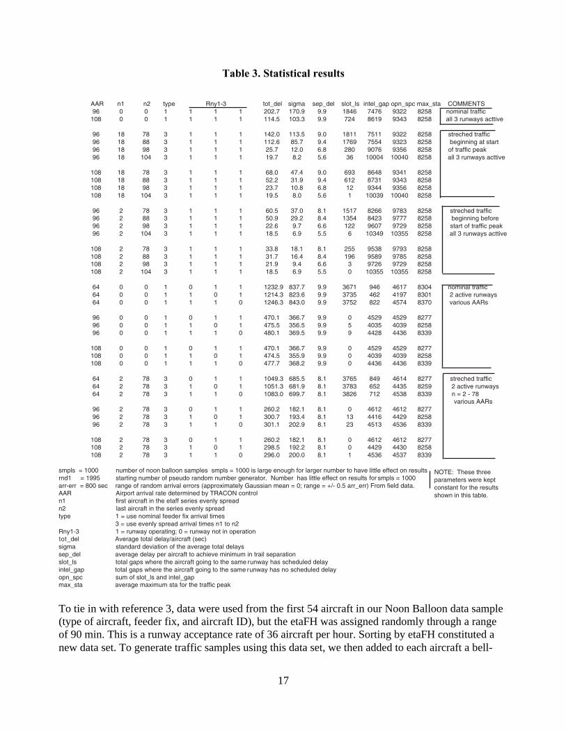
In order to study several other situations, we made other runs while providing minimum outputs.Forty-eight runs were made of 1,000 traffic samples—each to explore the performance of thedifferent aspects and methods of airline scheduling in interaction with the TMA scheduler (seetable 3, page 17). For comparison of the results, we used the same starting pseudorandom numberfor all tests. At this number of samples, the starting value of the pseudorandom number generatormade negligible difference in the outcome of the tests (not shown). In addition, all the tests shown intable 3 were run with a smaller arrival-error range of 200 sec. This change made very littledifference in the outcomes, although the average Center delay was usually a few seconds smaller forthe narrower error range.

16

The first 18 tests are concerned with all three runways in operation. In lines 1 and 2 of table 3, theresponse of the TMA to original traffic is compared for the two typical TRACON-commandedarrival rates. For the larger AAR = 108, the average Center delay is almost reduced to half, and thevariations between samples (sigma) are substantially reduced with increased AAR, as is the slot loss.The same tendency is true for all cases when the traffic is spread more evenly. The question is howoften does TRACON have to reduce its AAR when going from VFR to IFR? Although thesimulation does not prove this, it is likely that when the traffic is spread more uniformly, TRACONcan handle the traffic more easily, thus making an improved assignment of arrival times even moredesirable.

Two methods of traffic-slot assignments were investigated: (1) choose equal separation when thetraffic begins to get dense and increase the traffic density somewhat when originally it is light (rows3 to 10, table 3), or (2) in addition, increase the traffic density when the traffic is light before thebeginning of the traffic peak and after it is light again (rows 11 to 18), so that we have an increasedinitial and final arrival rate when compared with the original traffic. This is compensated for by alower, more uniform arrival rate during the time of the original peak traffic. The second method ismore advantageous to the airlines as was discussed in detail in the last section. In both cases the slotloss decreases as the average traffic becomes less dense and the gaps increase.

We also investigated original scheduling and scheduling with assigned slots when only two runwaysare operating (rows 19 to 36, table 3). Of course, the TMA scheduled delays will increasedrastically, but the evenly spaced scheduling from n = 2 to n = 78 still shows a definite advantageover the original schedule. Compressing the early, widely spaced arrivals reduces the delays in thesecond case. This is similar but more effective than the time advance explored in reference 1. Fromthe last column of table 3 (max_sta), it can be seen that the last scheduled aircraft (n = 111) is neverdelayed, which means that delays between traffic peaks are still independent. This was not the casewhen an attempt was made to schedule the traffic to a single runway.

Comparing the six sets of three rows each (rows 19 to 36, table 3), which are concerned with onlytwo runways in operation, it is noted that the order of the Center delay magnitudes remain the samefor any combination of the active runways. Also, for conditions that are otherwise the same, thedelays do not change very much as a function of the active runways. Too low a choice of AARtriples the total delays. But, increasing the AAR past 96 has no affect on the outcomes. This happensbecause at that point the airport’s two runways are fully utilized; that is, all aircraft on both runwaysare separated by their specified minimum time interval.

Various other pieces of information are given concerning the various gaps in the schedule. For allcases, when three runways are used, the slot-loss decreases with increased spread (n1 – n2) and itdecreases with increased AAR. This is true also for the case of two runways in use, although here itwould not be useful to reduce the AAR to a lower value.

Interaction Between Center and TRACON Scheduling

The interactions between the parameters AAR and the delay distribution dTmax on the overallscheduling results are somewhat complicated. So simpler examples will be discussed first.

17

Table 3. Statistical results

AAR n1 n2 type Rny1-3 tot_del sigma sep_del slot_ls intel_gap opn_spc max_sta COMMENTS

96 0 0 1 1 1 1 202.7 170.9 9.9 1846 7476 9322 8258 nominal traffic 108 0 0 1 1 1 1 114.5 103.3 9.9 724 8619 9343 8258 all 3 runways acttive

96 18 78 3 1 1 1 142.0 113.5 9.0 1811 7511 9322 8258 streched traffic 96 18 88 3 1 1 1 112.6 85.7 9.4 1769 7554 9323 8258 beginning at start 96 18 98 3 1 1 1 25.7 12.0 6.8 280 9076 9356 8258 of traffic peak 96 18 104 3 1 1 1 19.7 8.2 5.6 36 10004 10040 8258 all 3 runways acttive

108 18 78 3 1 1 1 68.0 47.4 9.0 693 8648 9341 8258 108 18 88 3 1 1 1 52.2 31.9 9.4 612 8731 9343 8258 108 18 98 3 1 1 1 23.7 10.8 6.8 12 9344 9356 8258 108 18 104 3 1 1 1 19.5 8.0 5.6 1 10039 10040 8258

96 2 78 3 1 1 1 60.5 37.0 8.1 1517 8266 9783 8258 streched traffic 96 2 88 3 1 1 1 50.9 29.2 8.4 1354 8423 9777 8258 beginning before 96 2 98 3 1 1 1 22.6 9.7 6.6 122 9607 9729 8258 start of traffic peak 96 2 104 3 1 1 1 18.5 6.9 5.5 6 10349 10355 8258 all 3 runways acttive

108 2 78 3 1 1 1 33.8 18.1 8.1 255 9538 9793 8258 108 2 88 3 1 1 1 31.7 16.4 8.4 196 9589 9785 8258 108 2 98 3 1 1 1 21.9 9.4 6.6 3 9726 9729 8258 108 2 104 3 1 1 1 18.5 6.9 5.5 0 10355 10355 8258

64 0 0 1 0 1 1 1232.9 837.7 9.9 3671 946 4617 8304 nominal traffic 64 0 0 1 1 0 1 1214.3 823.6 9.9 3735 462 4197 8301 2 active runways 64 0 0 1 1 1 0 1246.3 843.0 9.9 3752 822 4574 8370 various AARs

96 0 0 1 0 1 1 470.1 366.7 9.9 0 4529 4529 8277 96 0 0 1 1 0 1 475.5 356.5 9.9 5 4035 4039 8258 96 0 0 1 1 1 0 480.1 369.5 9.9 9 4428 4436 8339

108 0 0 1 0 1 1 470.1 366.7 9.9 0 4529 4529 8277 108 0 0 1 1 0 1 474.5 355.9 9.9 0 4039 4039 8258 108 0 0 1 1 1 0 477.7 368.2 9.9 0 4436 4436 8339

64 2 78 3 0 1 1 1049.3 685.5 8.1 3765 849 4614 8277 streched traffic 64 2 78 3 1 0 1 1051.3 681.9 8.1 3783 652 4435 8259 2 active runways 64 2 78 3 1 1 0 1083.0 699.7 8.1 3826 712 4538 8339 n = 2 - 78

various AARs 96 2 78 3 0 1 1 260.2 182.1 8.1 0 4612 4612 8277 96 2 78 3 1 0 1 300.7 193.4 8.1 13 4416 4429 8258 96 2 78 3 1 1 0 301.1 202.9 8.1 23 4513 4536 8339

108 2 78 3 0 1 1 260.2 182.1 8.1 0 4612 4612 8277 108 2 78 3 1 0 1 298.5 192.2 8.1 0 4429 4430 8258 108 2 78 3 1 1 0 296.0 200.0 8.1 1 4536 4537 8339

smpls = 1000 number of noon balloon samples smpls = 1000 is large enough for larger number to have little effect on resultsrnd1 = 1995 starting number of pseudo random number generator . Number has little effect on results arr-err = 800 sec range of random arrival errors (approximately Gaussian mean = 0; range = +/- 0.5 arr_err) From field data.AAR Airport arrival rate determined by TRACON control n1 first aircraft in the etaff series evenly spread n2 last aircraft in the series evenly spreadtype 1 = use nominal feeder fix arrival times 3 = use evenly spread arrival times n1 to n2 Rny1-3 1 = runway operating; 0 = runway not in operation

t_del Average total delay/aircraft (sec) sigma standard deviation of the average total delayssep_del average delay per aircraft to achieve minimum in trail separation slot_ls total gaps where the aircraft going to the same unway has scheduled delayintel_gap total gaps where the aircraft going to the same unway has no scheduled delayopn_spc sum of slot_ls and intel_gapmax_sta average maximum sta for the traffic peak

to

smpls = 1000forNOTE: These three parameters were kept constant for the results shown in this table.

rr

To tie in with reference 3, data were used from the first 54 aircraft in our Noon Balloon data sample(type of aircraft, feeder fix, and aircraft ID), but the etaFH was assigned randomly through a rangeof 90 min. This is a runway acceptance rate of 36 aircraft per hour. Sorting by etaFH constituted anew data set. To generate traffic samples using this data set, we then added to each aircraft a bell-

18

shaped uncertainty to the freeze-horizon arrival times with zero mean and 800-sec range. In addition,a ±180-sec feeder-fix arrival error was assumed, it too with a bell-shaped distribution. (This differsfrom the example in ref. 3, where each sample was generated by randomly assigning 54 aircraftthrough the 90-min range.)

To study the efficiency of the multiple runway scheduler, it was of interest also to simulate two orthree times the number of aircraft, as well as runways during the same time interval of 90 min. Asshown in figure 13, changing the feeder-fix arrival errors from a range of ±180 sec to 0 gave arelatively small percentage improvement of ∆DOC, which was largest for small dTmax. The single-runway curve for the nominal feeder-fix arrival errors in figure 13 has a minimum at dTmax of 180.The two runway curves have a weak minimum at dTmax = 270, and the three runway curves flattenout to a constant value at high dTmax, when all delays are taken in TRACON. Of more interest isthe difference between the one-, two-, and three-runway minimum ∆DOC’s. The optimization of therunway selection has reduced the ∆DOC’s considerably for more runways, even though the originaltraffic density per runway was the same.

In the remainder of this section, the Noon Balloon is studied and compared with its squared version.Because of the small effect on the results, there is only mild concern with improvements obtainedwhen the feeder-fix arrival error is reduced. Fortunately, in understanding the scheduling processesand the results, it is not necessary to be immediately concerned with the ∆DOC-results. Once theoutcomes of various strategies have been computed in terms of the actual scheduled delays in Centerand TRACON while using the fast-time simulation, the various ∆DOC’s can be computed in onestep by applying the different forms of the ∆DOC equations.

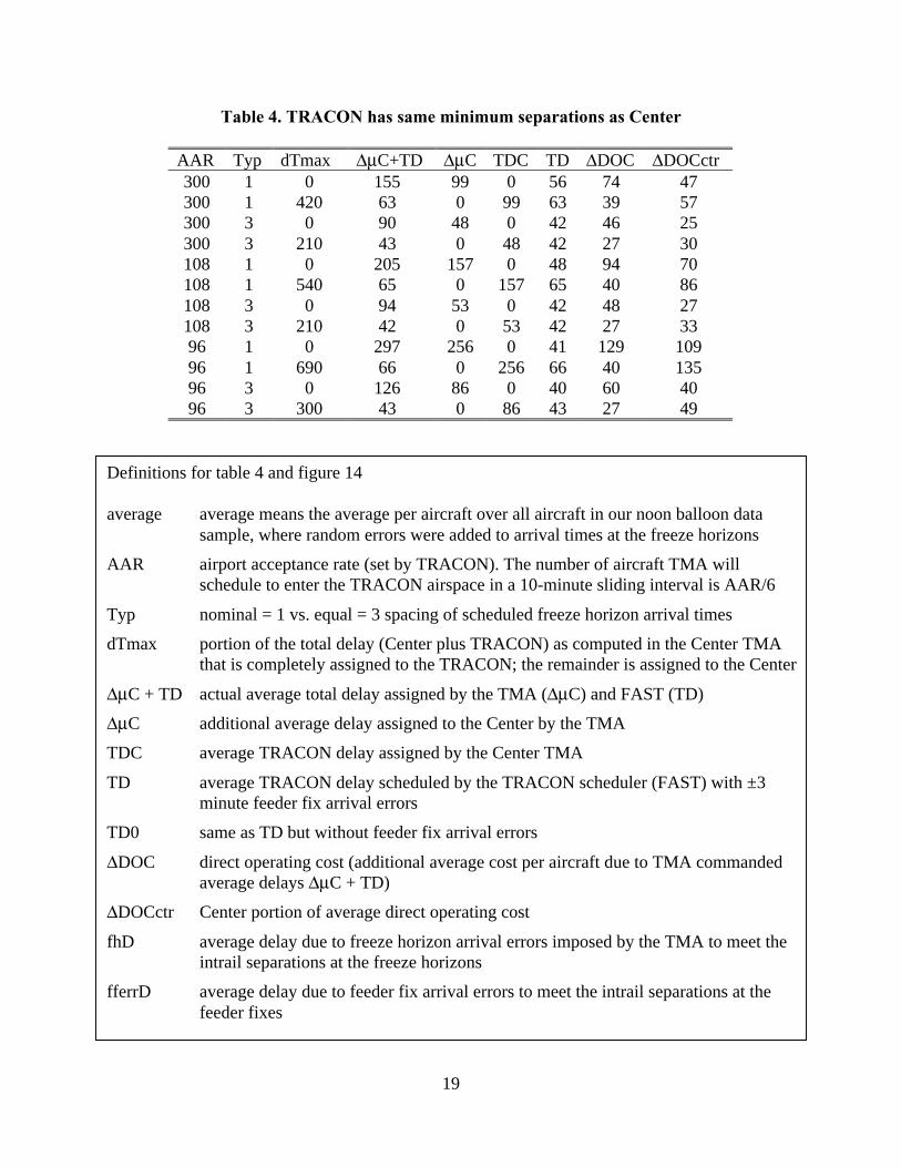
To understand the somewhat unexpected outcomes, the original Noon Balloon scheduling is firstexamined when the traffic is not AAR-limited (see fig. 14(a) for various dTmax). Definitions for theparameters in figure 14 and table 4 appear in the box following table 4. From the view of the Centerscheduler, which originally schedules to the runway, the Delay Distribution Function divides thetotal delay for each aircraft in such a manner that the average total delay is a certain constant valueindependent of dTmax (∆µC + TDC = constant (not shown)), which makes the resulting scheduledtouchdown times for each aircraft independent of dTmax. As a function of increasing dTmax, theaverage TMA scheduled Center delay (∆µC) always decreases from a maximum value to zero, andthe TMA scheduled TRACON delay does the reverse (TDC).

We will demonstrate this by means of comb diagrams at a later time. Similarly, as a function ofincreasing dTmax, the TRACON delay computed inside TRACON (TD) always increases from aminimum value (greater than zero) to a maximum constant value, after the delays for all trafficsamples have been transferred to the TRACON. The three delays ∆µC + TD, TD, and TDC allconverge to constant values, once all delays are taken in the TRACON. From then on, the Centerdelay remains zero except for fhD and fferrD, the delays that need to be imposed to meet the in-trailseparations at the freeze horizons and the feeder fixes, and these are small. These statements aretrue, independent of other parameters such as AAR or the type of airline schedule used. Figure 14(a)shows the curve for TD with the feeder-fix arrival error ±3-min in order to compare it with TD0, thecurve for no such error. The differences are small, and this curve is omitted from further graphs ofthis kind. Figure 14(b) for the squared Noon Balloon looks similar to 14(a), but there are twoprominent differences: the TDC at large dTmax is about one-half of that in figure 14(a), and dTmaxat which all delay is absorbed in the TRACON is also much smaller.

19

Table 4. TRACON has same minimum separations as Center

AAR Typ dTmax ∆µC+TD ∆µC TDC TD ∆DOC ∆DOCctr300 1 0 155 99 0 56 74 47300 1 420 63 0 99 63 39 57300 3 0 90 48 0 42 46 25300 3 210 43 0 48 42 27 30108 1 0 205 157 0 48 94 70108 1 540 65 0 157 65 40 86108 3 0 94 53 0 42 48 27108 3 210 42 0 53 42 27 3396 1 0 297 256 0 41 129 10996 1 690 66 0 256 66 40 13596 3 0 126 86 0 40 60 4096 3 300 43 0 86 43 27 49

Definitions for table 4 and figure 14

average average means the average per aircraft over all aircraft in our noon balloon datasample, where random errors were added to arrival times at the freeze horizons

AAR airport acceptance rate (set by TRACON). The number of aircraft TMA willschedule to enter the TRACON airspace in a 10-minute sliding interval is AAR/6

Typ nominal = 1 vs. equal = 3 spacing of scheduled freeze horizon arrival times

dTmax portion of the total delay (Center plus TRACON) as computed in the Center TMAthat is completely assigned to the TRACON; the remainder is assigned to the Center

∆µC + TD actual average total delay assigned by the TMA (∆µC) and FAST (TD)

∆µC additional average delay assigned to the Center by the TMA

TDC average TRACON delay assigned by the Center TMA

TD average TRACON delay scheduled by the TRACON scheduler (FAST) with ±3minute feeder fix arrival errors

TD0 same as TD but without feeder fix arrival errors

∆DOC direct operating cost (additional average cost per aircraft due to TMA commandedaverage delays ∆µC + TD)

∆DOCctr Center portion of average direct operating cost

fhD average delay due to freeze horizon arrival errors imposed by the TMA to meet theintrail separations at the freeze horizons

fferrD average delay due to feeder fix arrival errors to meet the intrail separations at thefeeder fixes

20

Since the equivalent figures to figure 14 all have the same character, the data are presented intable 4, where Typ = 0 is for the nominal and Typ = 3 for the squared Noon Balloon, and ∆DOCctris the ∆DOC calculated for single-step scheduling based on the Center TMA data only. It can beseen for dTmax > 0, that the lower the AAR, the higher must be dTmax for a given type ofscheduling to accommodate all delays in the TRACON. For each particular AAR and type, ∆DOC isalways smallest for the large dTmax. The smallest ∆DOCctr is the one for dTmax = 0, since less fuelis used when the aircraft spends more time in the Center.

To gain a better insight into the behavior of the curves shown in figure 14, somewhat simplifiedcomb diagrams are studied for one specific traffic sample at the extreme values of dTmax (0 and450). Figures 15(a) and 15(b) show the diagrams from the view of the Center scheduling, where alldelays are either at the Center or in the TRACON. We can see that the scheduled STAs are identicalfor both figures. However, the STAff values that the TRACON scheduler has to deal with aresmaller in the case of large dTmax. Hence, we can expect smaller TRACON scheduled touchdowntimes for the latter case. This is shown in figures 16(a) and 16(b). The individual changes arerelatively small, hence the delay changes are also plotted for individual aircraft in figure 17. Finally,a comparison is made between total delays (∆µC + TD) of 100 samples with identical initialconditions but with the extreme dTmax’s. In addition, figure 18 shows the comparison for anintermediate dTmax = 150. There is an overlap between Noon Balloon samples at dTmax 150 and480, but more often than not the results for larger dTmax show lower delays. It can be seen fromfigure 18 that individual traffic samples have quite a range of average total delays, and that dTmax =480 compared to dTmax = 0 always has the lowest delay for identical incoming traffic.

It may be of interest to know what the reassignment of runways accomplishes, given whatever theATAff’s are (eta3 order versus etaff order). The results are shown in figure 19. The figure showsthat the scheduling in eta3 order is advantageous for all values of dTmax. We have also testedremoving just the eta3 ordering for the Center scheduler, or for both Center and TRACONschedulers. The results are shown in figure 19. The lowest ∆DOC always occurs when both runwayoptimizers are active.

Since, ordinarily, we have feeder-fix arrival errors, and the TRACON scheduler reschedules eachair cr af t , includi ng a new r unway sel ect ion, the new t ot al del ay, the sum of t he Cent er and the sched-uled delays inside TRACON (∆µC + TD), does not remain constant, but starts with a value for lowdTm ax considerabl y higher t han t he t otal del ay comput ed fr om the Center per spect ive (∆ µ C + T DC) .

Center delay is defined here as the sum of the actual delay in the Center (dc), plus the arrival errorsat the freeze horizon (fhD), and the arrival errors at the feeder fixes (fferrD):

dC = dc +fhD + fferrD (sec) (6)

For convenience, equation (3) on page 9 is repeated here:

∆DOC = dC(CT + 2CF) + kdT(CT + 3CF) ($) (3)

21

These two equations show that decreasing variable dC and increasing variable dT with dTmaxmultiplied by different constants results in a constant ∆DOC for large dTmax. In all cases examined,∆DOC initially decreases with increasing dTmax. Hence, there are two possibilities: the firstminimum value occurs before all delay is transferred to the TRACON or at the point where all delayis absorbed in the TRACON airspace.

Figures 20(a) and 20(b) are for AAR = 300, with feeder-fix arrival errors. The resulting DOC isstudied for different assumptions to indicate the sensitivity to different economical changes:

1. Nominal ∆DOC including costs to compensate for freeze-horizon and feeder-fix arrival errors

2. Doubling the fuel cost

3. Calculating the ∆DOC as seen by the TMA

Just as in the single-runway case (similar to reference 3), there exists a weak minimum ∆DOCbefore all delays (except for the delays that must be taken in the Center to meet the separationrequirements at the freeze horizons and at the feeder fixes), are assigned to the TRACON only in thecase where the cost inside TRACON being quadrupled led from the nominal (k = 4 in eq. (3), curvenot shown in fig. 20). For the squared Noon Balloon and realistic feeder-fix arrival errors, we againhave to wait for the plateau, when all possible delays are assigned to the TRACON, to minimize thedifferential cost. Comparing the figures for both nominal the Noon Balloon and the squared version,figures 20(a) and 20(b), it is seen that substantial reductions occur in ∆DOCs for the squared NoonBalloon over the nominal version. Figures 20(a) and 20(b) show plots of the ∆DOC for the single-step case in which all possible delays are calculated in the Center. For these cases, cost is smallest atdTmax = 0, and increases as more time is spent in TRACON.

Table 4 already recorded the effect of limiting traffic flow into the TRACON by means of the AAR.In all cases the ∆DOC and minimal total delays occurred when all possible scheduled delays weretransferred to the TRACON. This gave the somewhat surprising result that the highest average delayfor the smallest AAR was obtained for both the nominal and the squared Noon Balloon. However,when the optimal total delays and ∆DOCs were compared for the combined system, which reassignsrunways and recalculates ∆DOCs after feeder-fix crossing, they are only weakly dependent on theAAR, provided that dTmax is chosen so that all delays are assigned to the TRACON. It is also notedthat the required dTmax is much smaller for the squared version of the traffic peak than for thenominal version. To further understand this, figures 21(a) and 21(b) show the histograms for thenominal and squared Noon Balloon of individual aircraft delays for 1,000 data samples (1,000 x 111aircraft/sample = 111.000 aircraft) for the individual delays for all three AAR. As can be seen, thereis very little difference between the results for the AAR. The original peaks of 43,000 and 53,000aircraft with small delays is mostly a result of the initial peak traffic followed by sparse traffic in thetime interval we studied. Comparison of figures 21(a) and 21(b) shows the advantage of squaring theNoon Balloon traffic.

22

CONCLUDING REMARKS

We have shown that fast-time simulation (FTS) has certain benefits and requirements:

1. One of the keys to a valid FTS is to build a computer model of the system that is to be studied. Inthe case of the TMA, many details such as aircraft dynamics and weather models had to beomitted. This means that we cannot make any experiments involving these variables. To build auseful model, it is important to work closely with the system designers.

2. With FTS we explored system performances over a range of initial conditions, as well as randomdisturbances, since we had the proper models for these variables from field tests. Such testswould be difficult using full-scale, real-time simulations of the TMA.

3. Graphical representations, as well as intermediate printouts of the results, were very important inchecking results. For instance, the comb diagram was very helpful in spotting errors in the code,as was the printout of runway balancing.

4. Another aspect of the FTS model, which is a simplification of the real TMA, is that it must notbe used beyond the capability of the actual system. For example, in the FTS model, we treatedall aircraft information as one sequence that could be manipulated as a whole. In actual traffic,aircraft appear sequentially, and scheduling has to be performed on partial sequences. Thus aninvestigation such as described in the section titled Earlier Studies of Fast-Time Simulationwould be valid. Another method of reducing delays consists of going through the schedulingprocess several times, each time using the last results as a start, and stopping when the nextiteration gave a higher delay. This would be a nonvalid use of the FTS simulation for the abovereasons.

5. An advantage of FTS of the TMA was that no deep knowledge of statistics was required. Onecan simply run enough samples until the output is essentially independent of the sample size.

6. FTS had a large payoff in terms of useful insight acquired and in the speed with which it wasobtained.

7. Since some of the fine details of the actual system have not been implemented, the results areonly an approximation of the actual TMA performance.

8. Theoretically it is, of course, possible to use the complete TMA program and to automate themanned simulation by replacing the pseudopilots and controllers with simulations, and then torun the system with computer-generated traffic samples in faster than real time. Except for thedifficulties of writing programs that simulate the situational awareness of controllers, and theresulting controller commands to meet the scheduled arrival times, as well as simulatingcontroller, pilot, and aircraft interactions, this would be another approach for checking out thecomplete TMA program and its performance before installing it at an airport.

23

REFERENCES

1. Neuman, F.: Analysis of Sequencing and Scheduling Methods for Arrival Traffic. NASA TM-102795, April 1990.

2. Neuman, F.: Analysis of Delay Reducing and Fuel Saving Sequencing and Spacing Algorithmsfor Arrival Traffic. NASA TM-103880, 1991.

3. Erzberger, H.: Design Principles and Algorithms for Automated Air Traffic Management. Paperpresented at the Mission Systems Panel of AGARD, Nov. 1995.

4. Carr, G. C.; Erzberger, H.; and Neuman, F.: Delay Exchanges in Arrival Sequencing andScheduling. J. Aircraft, vol. 36, no. 5, Sept./Oct. 1999.

5. Carr, G. C.; Erzberger, H.; and Neuman, F.: Fast Time Study of Airline Influenced ArrivalSequencing and Scheduling. J. Guidance and Dynamics, vol. 23, no. 3, May/June 2000.

6. Wong, G. L.: The Dynamic Planner: The Sequencer, Scheduler, and Runway Allocator for AirTraffic Control Automation. NASA TM-209586, April 2000.

7. Ott, James: American Takes a Risk with Rolling Hub. Avia. Week & Space Tech., vol. 157, no.10, Sept. 2, 2002, pg. 26.

8. Hoffman, R. and Ball, M.: Measuring Ground Delay Program Effectiveness Using the RateControl Index. Nextor Publications (2000), NR-2000-002, June 2000.(Available from http://www.metronaviation.com/cdm/analysis/nextor_reports.html)

9. Vossen, T. and Ball, M.: Optimization and Mediated Bartering Models for Ground DelayPrograms. Nextor Publications (2001), NR-2001-005, Aug. 2001.(Available from http://www.metronaviation.com/cdm/analysis/nextor_reports.html)

10. Willemain, T. R.: Contingencies and Cancellations in Ground Delay Programs. Nextor WorkingPapers, NWP-2001-003, May 2001.(Available from http://www.isr.umd.edu/NEXTOR/pubs/WP-01-3.pdf)

24

25

Establish new order foreach stream class due

to FH arrival errors

Print out informationabout the parameters of

the data samples

Calculate for each aircrafteta’s to each runway:

eta0, eta1, eta2

Establish scheduling order(eta3 order = minimum of

eta0, eta1, eta2)

staff

ataff

eta sta

N repetitions?Print out summary dataENDyes no

Push-back to keep original stafforder for each stream class while

creating a minimum 60 secseparation

Accumulate delay due to pushback

Model of feeder fixarrival errors

Airport model: feeder fix to runwaythreshold time =

t(type, feeder fix, runway)

TRACON scheduler schedules from actualarrival times at the feeder fix to a runway,using the same logic to select runways asthe Center scheduler except no AAR limit

and no delay distribution

Center Schedule: In eta3 orderschedule to each runway considering theaircraft just scheduled before. The runway

which gives the lowest landing time ischosen. Then backoff to the feeder fix

Minimum time of separationbetween the last scheduled

and next aircraft to bescheduled f(typ1st, typ2)

Print out average delaysover N samples.+histogram of averagesample delays in 30second intervals+individual aircraft delaysin 30 second intervals

eta31<eta32<eta33<...

etaxj

Input parameters:N = number of traffic samples

AAR = airport acceptance rate etc.

Noon Balloon field data:aircraftID(etaff_19, type, feeder fix, stream class

or modified etaff for smaller arrival delays

Model of freeze horizonarrival errors

Accumulate delay due to pushback

Note*etaff: estimated time of arrival, feeder fixstaff: scheduled time of arrival, feeder fixataff: actual time of arrival, feeder fixeta: estimated time of arrivalsta: scheduled time of arrivalata: actual time of arrival

Push-back to keep new etafforder for each stream class while

creating a minimum of 60 secseparation

Center scheduling processand data collection

Figure 1. Fast-time estimated arrival-time error distribution.

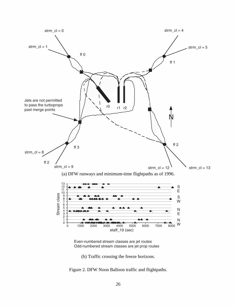
26

Jets are not permittedto pass the turbopropspast merge points

strm_cl = 8

strm_cl = 9

strm_cl = 1

strm_cl = 0 strm_cl = 4

strm_cl = 12 strm_cl = 13

ff 3

ff 0

ff 1

r0 r1 r2

ff 2

ff 2

strm_cl = 5

(a) DFW runways and minimum-time flightpaths as of 1996.

Even-numbered stream classes are jet routesOdd-numbered stream classes are jet prop routes

Str

eam

cla

ss

SE

SW

NE

NW

etaff_19 (sec)

131211109876543210

0 1000 2000 3000 4000 5000 6000 7000 8000

(b) Traffic crossing the freeze horizons.

Figure 2. DFW Noon Balloon traffic and flightpaths.

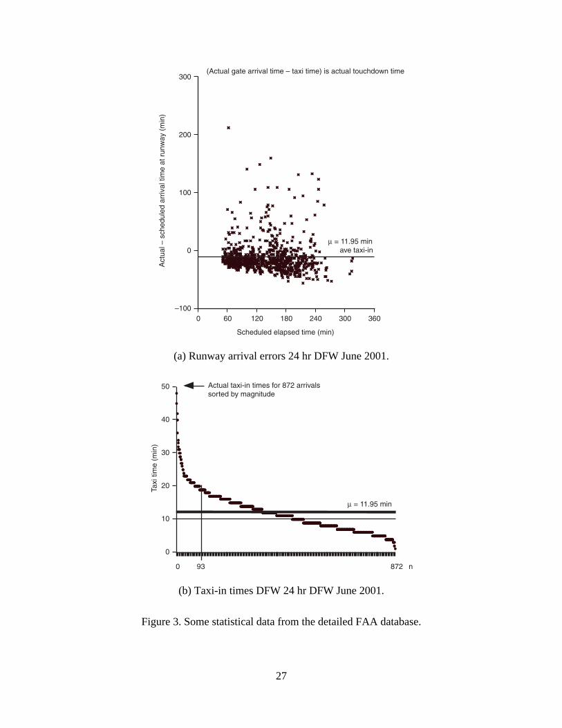
27

Act

ual –

sch

edul

ed a

rriv

al ti

me

at r

unw

ay (

min

)

Scheduled elapsed time (min)

µ = 11.95 minave taxi-in

300

200

100

0

0 60 120 180 240 300 360–100

(Actual gate arrival time – taxi time) is actual touchdown time

(a) Runway arrival errors 24 hr DFW June 2001.

µ = 11.95 min

50

40

30

20

10

0

0 93 872

Actual taxi-in times for 872 arrivalssorted by magnitude

n

Taxi

tim

e (m

in)

(b) Taxi-in times DFW 24 hr DFW June 2001.

Figure 3. Some statistical data from the detailed FAA database.

28

Line starts at the feeder fix the aircraft overflies

Tight scheduling

ff0

ff1

ff2

ff3

r0

r1r2

0 1000 2000 3000 4000

delayMinimum separationadjacent a/c on same runway (ft)

5000 6000 Time (sec)

(a) Comb diagram of Noon Balloon sample.

Difference in travel time to chosen runway and closest runway

Line kinks when closest runway not chosen

Vertical segment means no delay when flyingto the selected runwaythen:

Gap not counted as slot loss

Delay flying to selected runway

Total delay ff toselected runway

(b) Detailed description of logical content of figure 4(a).

Figure 4. The comb diagram and detailed explanation of its elements.

29

Num

ber

sche

dule

d8

7

6

5

4

3

2

1

5 A.M.300 600 900 1200 1500

Local time DFW (hours)

Time (minutes)

10 A.M. 3 P.M. 8 P.M. 1 A.M.

(a) Number of aircraft scheduled to arrive at the same minute versus time.

40

30

0

20

10

Time (minutes)

AAR 96AAR 108

5 A.M.300 600 900 1200 1500

10 A.M. 3 P.M. 8 P.M. 1 A.M.

Nub

er o

f airc

raft

in 1

0 m

in

Local time DFW

(b) Number of aircraft scheduled to arrive at DFW in sliding 10-min intervals as of 12 June, 2001.

Figure 5. Two representations of aircraft scheduling density at DFW on 12 June 2001.

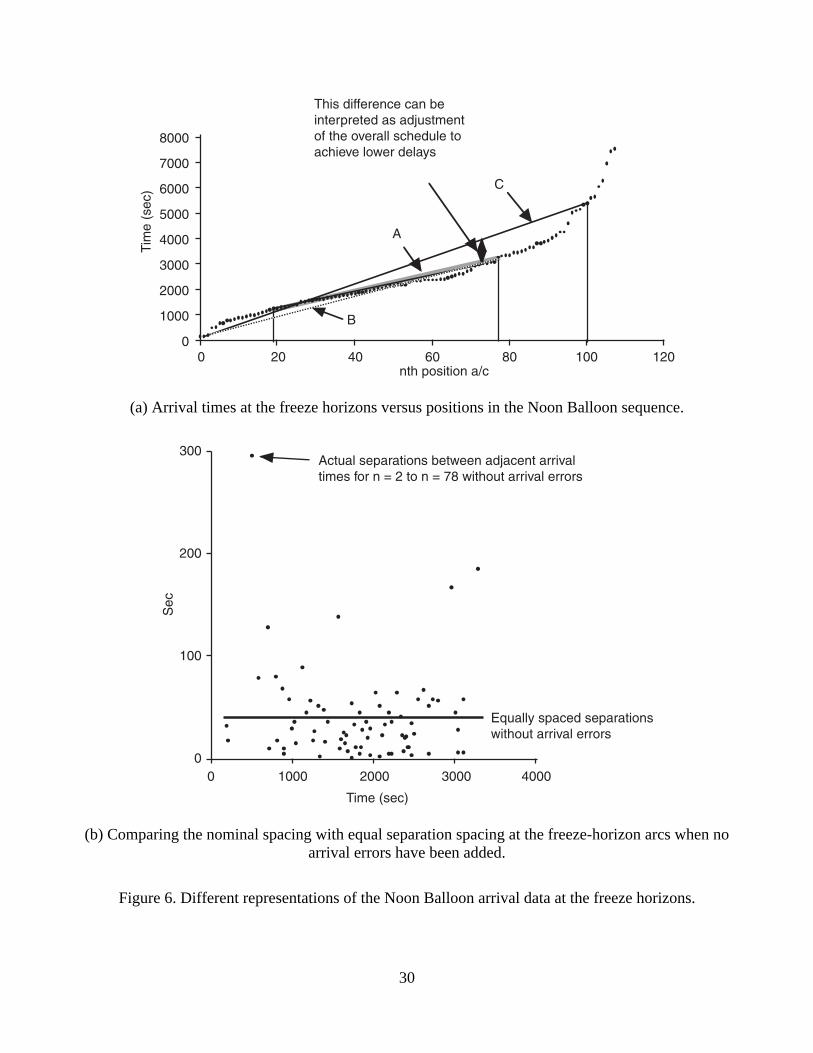
30

nth position a/c

Tim

e (s

ec)

8000

This difference can beinterpreted as adjustmentof the overall schedule toachieve lower delays

B

A

C

7000

6000

5000

4000

3000

2000

1000

00 20 40 60 80 100 120

(a) Arrival times at the freeze horizons versus positions in the Noon Balloon sequence.

Actual separations between adjacent arrivaltimes for n = 2 to n = 78 without arrival errors

Equally spaced separationswithout arrival errors

300

200

100

00 1000 2000 3000 4000

Sec

Time (sec)

(b) Comparing the nominal spacing with equal separation spacing at the freeze-horizon arcs when noarrival errors have been added.

Figure 6. Different representations of the Noon Balloon arrival data at the freeze horizons.

31

ff0

ff1

ff2

ff3

r0

r1

r2

1000 1500 2000 2500 3000 3500 4000 4500Time (sec)

(a) Nominal traffic only n = 2 to 78 shown.

ff0ff1ff2

ff3

r0

r1

r2

1000 1500 2000 2500 3000 3500 4000 4500Time (sec)

(b) n = 2 to 78 equally spread only n = 2 to 78 shown.

Figure 7. Comparison of samples of nominal scheduled traffic and equally spaced trafficincluding arrival errors.

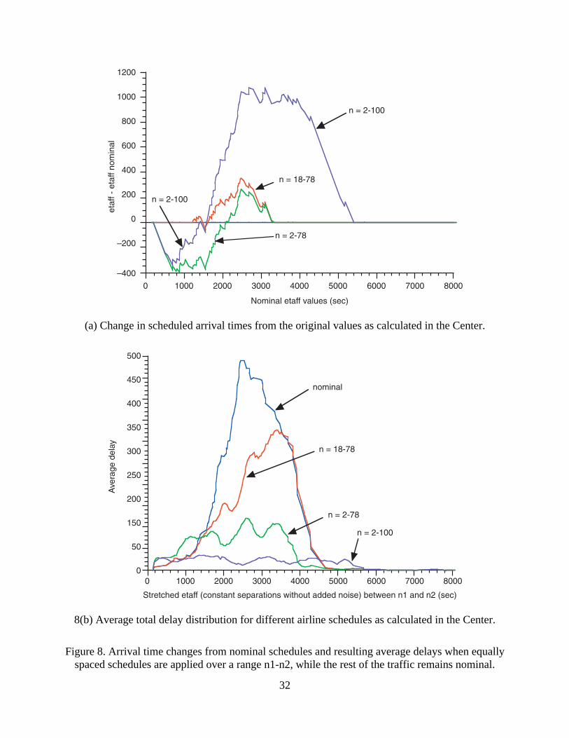
32

Nominal etaff values (sec)

0 1000 2000 3000

1200

1000

800

n = 2-100

n = 18-78

n = 2-100

n = 2-78

600

etaf

f - e

taff

nom

inal

400

200

0

–200

–400

4000 5000 6000 7000 8000

(a) Change in scheduled arrival times from the original values as calculated in the Center.

n = 18-78

n = 2-78

n = 2-100

500

450

400

350

300

250

200

150

50

0

Stretched etaff (constant separations without added noise) between n1 and n2 (sec)

0 1000 2000 3000 4000 5000 6000 7000 8000

Ave

rage

del

ay

nominal

8(b) Average total delay distribution for different airline schedules as calculated in the Center.

Figure 8. Arrival time changes from nominal schedules and resulting average delays when equallyspaced schedules are applied over a range n1-n2, while the rest of the traffic remains nominal.

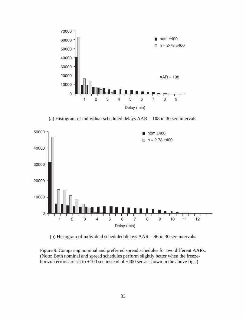
33

Delay (min)

1

70000

AAR = 108

60000

50000

40000

30000

20000

10000

02 3 4 5 6 7 8 9

n = 2-78 ±400

nom ±400

(a) Histogram of individual scheduled delays AAR = 108 in 30 sec-intervals.

Delay (min)

50000

40000

30000

20000

10000

01 2 3 4 5 6 7 8 9 10 11 12

n = 2-78 ±400

nom ±400

(b) Histogram of individual scheduled delays AAR = 96 in 30 sec-intervals.

Figure 9. Comparing nominal and preferred spread schedules for two different AARs.(Note: Both nominal and spread schedules perform slightly better when the freeze-horizon errors are set to ±100 sec instead of ±400 sec as shown in the above figs.)

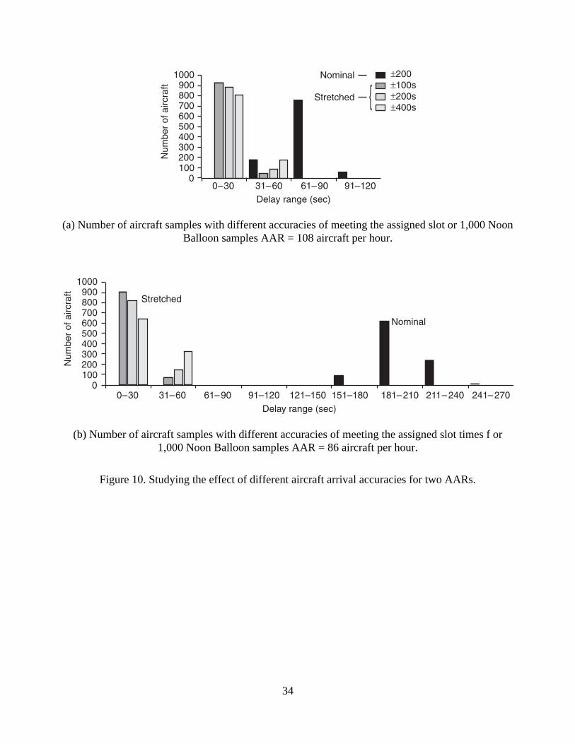
34

Num

ber

of a

ircra

ft

0–30

1000 Nominal ±200±100s±200s±400s

Stretched900800700600500400300200100

031–60 61–90 91–120

{

Delay range (sec)

(a) Number of aircraft samples with different accuracies of meeting the assigned slot or 1,000 NoonBalloon samples AAR = 108 aircraft per hour.

Stretched

Nominal

Num

ber

of a

ircra

ft

1000900800700600500400300200100

0

Delay range (sec)

0–30 31–60 61–90 91–120 121–150 151–180 181–210 211– 240 241– 270

(b) Number of aircraft samples with different accuracies of meeting the assigned slot times f or1,000 Noon Balloon samples AAR = 86 aircraft per hour.

Figure 10. Studying the effect of different aircraft arrival accuracies for two AARs.

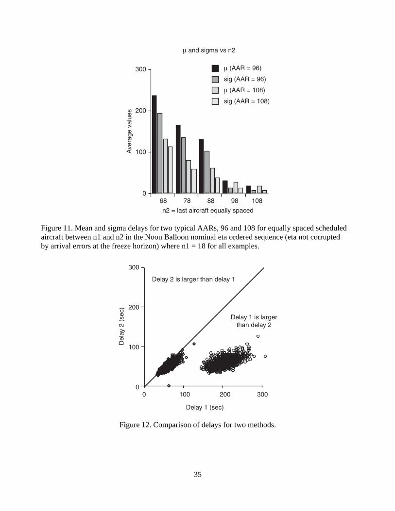
35

µ and sigma vs n2

n2 = last aircraft equally spaced

68 78 88 98 108

µ (AAR = 96)300

200

100

0

sig (AAR = 96)

µ (AAR = 108)

sig (AAR = 108)

Ave

rage

val

ues

Figure 11. Mean and sigma delays for two typical AARs, 96 and 108 for equally spaced scheduledaircraft between n1 and n2 in the Noon Balloon nominal eta ordered sequence (eta not corruptedby arrival errors at the freeze horizon) where n1 = 18 for all examples.

Delay 2 is larger than delay 1

Delay 1 is largerthan delay 2

Delay 1 (sec)

Del

ay 2

(se

c)

300

200

100

00 100 200 300

Figure 12. Comparison of delays for two methods.

36

∆DO

C

dTmax (sec)

275

250

225

200

175

1 runway 54 aircraft in 90 min

2 runways 108 aircraft in 90 min

3 runways 125 aircraft in 69.4 min

150

125

100

75

50

25

00 30 60 90 120 150 180 210 240 270 300 330 360 390 420 450

ff_arr_err = 360

ff_arr_err = 0

ff_arr_err = 360

ff_arr_err = 0

ff_arr_err = 360

ff_arr_err = 0

Figure 13. ∆DOC for N aircraft in 90 min all with the same density = runway arrival rate.(For three runways, time was reduced to give the same runway arrival rate.)

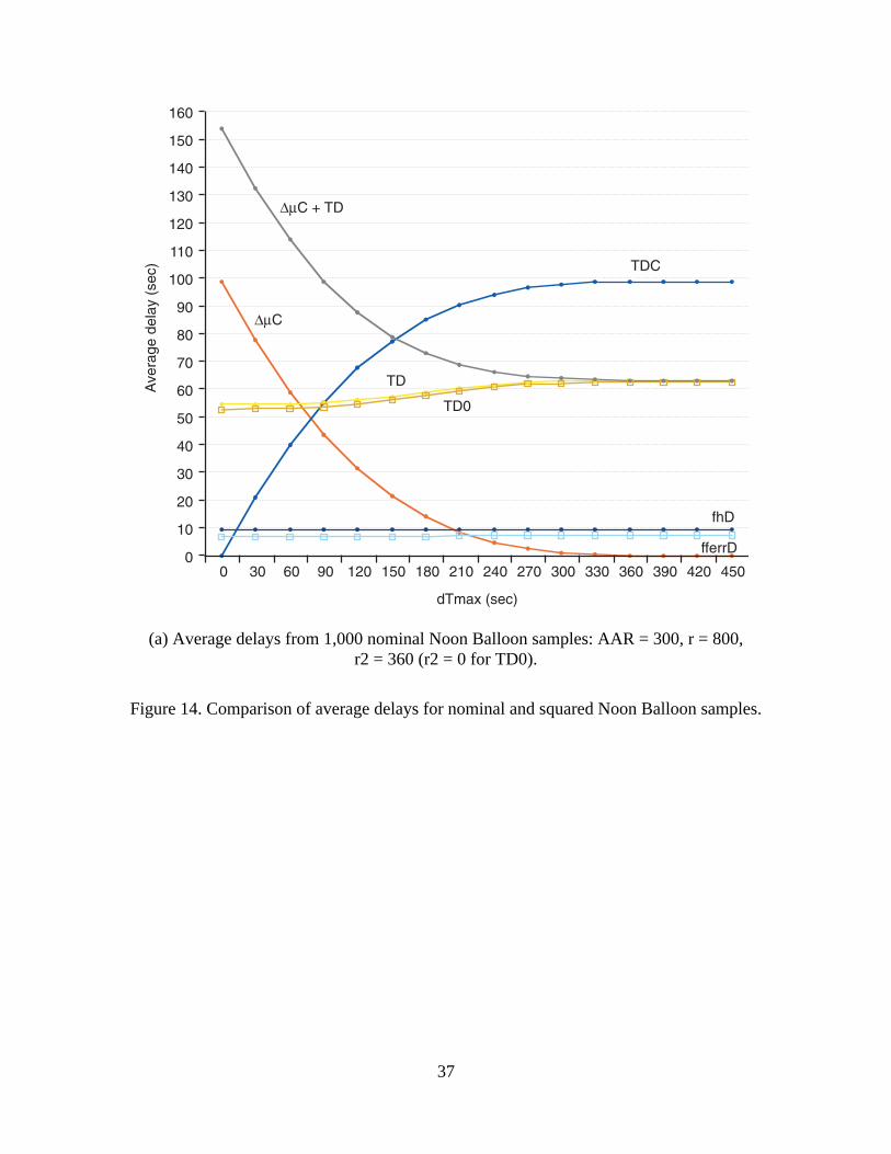
37

dTmax (sec)

0 30 60 90 120 150 180 210 240 270 300 330 360 390 420 450

Ave

rage

del

ay (

sec)

160

150

140

130

120

110

100

90

80

70

60

50

40

30

20

10

0

TD0

TD

fhD

fferrD

TDC

∆µC + TD

∆µC

(a) Average delays from 1,000 nominal Noon Balloon samples: AAR = 300, r = 800,r2 = 360 (r2 = 0 for TD0).

Figure 14. Comparison of average delays for nominal and squared Noon Balloon samples.

38

dTmax (sec)

0 30 60 90 120 150 180 210 240 270 300

Ave

rage

del

ay (

sec)

TD

fhD

fferrD

TDC

∆µC + TD

∆µC

100

90

80

70

60

50

40

30

20

10

0

(b) Average delays from 1,000 squared Noon Balloon samples: AAR = 300, r = 800, r2 = 360.

Figure 14. Concluded.

39

ff0

ff1

ff2

ff3

r0r1

r2

1000 1500 2000 2500 3000 3500 4000 4500

eta3

staff

sta

Time (sec)

(a) Center schedule: dTmax = 0.

ff0

ff1

ff2

ff3

r0r1

r2

1000 1500 2000 2500 3000 3500 4000 4500

eta3

staff

sta

Time (sec)

(b) Center schedule: dTmax = 450.

Figure 15. Center schedule for different dTmax.

40

1000

ff0ff1ff2ff3

r0r1r2

1500 2000 2500 3000 3500 4000 4500 5000

eta3

staff

sta

Time (sec)

(a) Center TRACON schedule: dTmax = 0.

ff0ff1ff2ff3

r0r1r2

1000 1500 2000 2500 3000 3500 4000 4500 5000

eta3

staff

sta

Time (sec)

(b) Center TRACON: dTmax = 450.

Figure 16. Schedule comparison for identical inputs (eta3) and different dTmax.

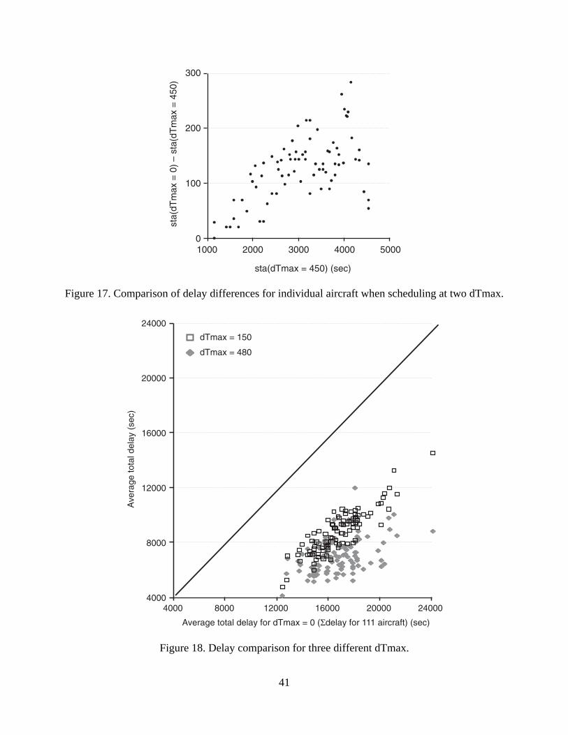
41

sta(

dTm

ax =

0)

– st

a(dT

max

= 4

50)

sta(dTmax = 450) (sec)

300

200

100

01000 2000 3000 4000 5000

Figure 17. Comparison of delay differences for individual aircraft when scheduling at two dTmax.

4000 8000 12000 16000 20000 240004000

8000

12000

16000

20000

24000

dTmax = 150

dTmax = 480

Average total delay for dTmax = 0 (Σdelay for 111 aircraft) (sec)

Ave

rage

tota

l del

ay (

sec)

Figure 18. Delay comparison for three different dTmax.

42

dTmax (sec)

0 30 60 90 120 150 180 210 240 270 300 330 360 390 420

∆DO

C

Center andTRACON etaff sort

Center eta3 sortTRACON etaff sort

Both eta3 sort

110

100

90

80

70

60

50

40

30

Figure 19. Demonstrating the advantage of scheduling in eta3 order in the Center and TRACON.

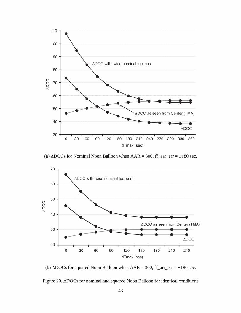
43

dTmax (sec)

0 30 60 90 120 150 180 210 240 270 300 330 360

∆DO

C

∆DOC with twice nominal fuel cost

∆DOC as seen from Center (TMA)

∆DOC

110

100

90

80

70

60

50

40

30

(a) ∆DOCs for Nominal Noon Balloon when AAR = 300, ff_aar_err = ±180 sec.

dTmax (sec)

0 30 60 90 120 150 180 210 240

∆DO

C

∆DOC with twice nominal fuel cost

∆DOC as seen from Center (TMA)

∆DOC

70

60

50

40

30

20

(b) ∆DOCs for squared Noon Balloon when AAR = 300, ff_arr_err = ±180 sec.

Figure 20. ∆DOCs for nominal and squared Noon Balloon for identical conditions

44

Num

ber

of a

ircra

ft w

ith d

elay

ran

ge

50000

40000

30000

20000

10000

0

AAR = 300AAR = 108AAR = 96

0 30 60 90 120 150 180 210 240 270 300 330 360

30-second delay ranges

(a) Nominal Noon Balloon.

30-second delay ranges

Num

ber

of a

ircra

ft

60000

50000

40000

30000

20000

10000

0

AAR = 300AAR = 108AAR = 96

0 30 60 90 120 150 180 210 240 270 300 330 360

(b) Squared Noon Balloon.

Figure 21. Comparison of TRACON delays for individual aircraft when all delays are transferred toTRACON (Center delay = 0 for large dTmax).

45

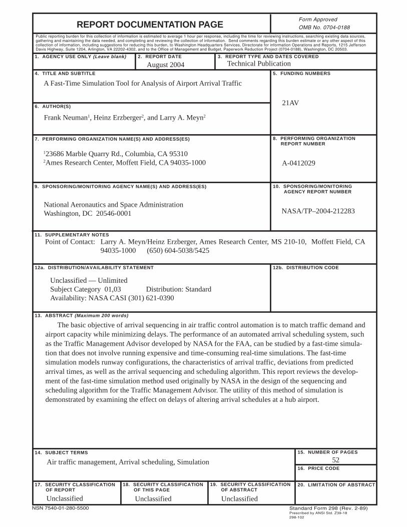
REPORT DOCUMENTATION PAGE

8. PERFORMING ORGANIZATION REPORT NUMBER

10. SPONSORING/MONITORING AGENCY REPORT NUMBER

Form Approved

OMB No. 0704-0188

12b. DISTRIBUTION CODE12a. DISTRIBUTION/AVAILABILITY STATEMENT

7. PERFORMING ORGANIZATION NAME(S) AND ADDRESS(ES)

4. TITLE AND SUBTITLE 5. FUNDING NUMBERS

6. AUTHOR(S)

1. AGENCY USE ONLY (Leave blank)

9. SPONSORING/MONITORING AGENCY NAME(S) AND ADDRESS(ES)

2. REPORT DATE 3. REPORT TYPE AND DATES COVERED

15. NUMBER OF PAGES

16. PRICE CODE

20. LIMITATION OF ABSTRACT19. SECURITY CLASSIFICATION OF ABSTRACT

18. SECURITY CLASSIFICATION OF THIS PAGE

17. SECURITY CLASSIFICATION OF REPORT

14. SUBJECT TERMS

13. ABSTRACT (Maximum 200 words)

Standard Form 298 (Rev. 2-89)Prescribed by ANSI Std. Z39-18298-102

NSN 7540-01-280-5500

Public reporting burden for this collection of information is estimated to average 1 hour per response, including the time for reviewing instructions, searching existing data sources,gathering and maintaining the data needed, and completing and reviewing the collection of information. Send comments regarding this burden estimate or any other aspect of thiscollection of information, including suggestions for reducing this burden, to Washington Headquarters Services, Directorate for information Operations and Reports, 1215 JeffersonDavis Highway, Suite 1204, Arlington, VA 22202-4302, and to the Office of Management and Budget, Paperwork Reduction Project (0704-0188), Washington, DC 20503.

11. SUPPLEMENTARY NOTES

Unclassified Unclassified

Unclassified — UnlimitedSubject Category 01,03 Distribution: StandardAvailability: NASA CASI (301) 621-0390

A-0412029

NASA/TP–2004-212283

August 2004

123686 Marble Quarry Rd., Columbia, CA 953102Ames Research Center, Moffett Field, CA 94035-1000

National Aeronautics and Space AdministrationWashington, DC 20546-0001

21AV

52

A Fast-Time Simulation Tool for Analysis of Airport Arrival Traffic

Frank Neuman1, Heinz Erzberger2, and Larry A. Meyn2

The basic objective of arrival sequencing in air traffic control automation is to match traffic demand andairport capacity while minimizing delays. The performance of an automated arrival scheduling system, suchas the Traffic Management Advisor developed by NASA for the FAA, can be studied by a fast-time simula-tion that does not involve running expensive and time-consuming real-time simulations. The fast-timesimulation models runway configurations, the characteristics of arrival traffic, deviations from predictedarrival times, as well as the arrival sequencing and scheduling algorithm. This report reviews the develop-ment of the fast-time simulation method used originally by NASA in the design of the sequencing andscheduling algorithm for the Traffic Management Advisor. The utility of this method of simulation isdemonstrated by examining the effect on delays of altering arrival schedules at a hub airport.

Air traffic management, Arrival scheduling, Simulation

Technical Publication

Point of Contact: Larry A. Meyn/Heinz Erzberger, Ames Research Center, MS 210-10, Moffett Field, CA94035-1000 (650) 604-5038/5425

Unclassified